von karman institute for fluid dynamics chaussee de...
TRANSCRIPT

Von Karman Institute for Fluid Dynamics Chaussee de Waterloo, 72 B- 1640 Rhode Saint Genese - Belgium
Project Report 1999 June 1999
Liquid Film Instabilities of Wire Coatings
S. Zuccher
Supervisor: J-M. Buchlin
Table of Contents
Abstract ........................................................................................................ iv Acknowledgements ....................................................................................... v List of symbols............................................................................................. vi List of figures .............................................................................................viii 1. Introduction .................................................................................................. 1
1.1 Introduction ................................................................................................................................1 1.2 Origin of the project ..................................................................................................................1 1.3 Objectives of the project ...........................................................................................................2 1.4 Contents of the project..............................................................................................................4
2. Wire coating process ..................................................................................... 5
2.1 Introduction ................................................................................................................................5 2.2 Simple withdrawal ......................................................................................................................5
2.2.1 Governing equations ......................................................................................................6 2.3 Die coating ..................................................................................................................................8
2.3.1 Governing equations ......................................................................................................8 2.4 Annular jet wiping ....................................................................................................................12
2.4.1 Governing equations ....................................................................................................12 3. Wire coating instabilities..............................................................................15
3.1 Introduction ..............................................................................................................................15 3.2 Problem formulation................................................................................................................16
3.2.1 Basic flow.......................................................................................................................17 3.2.2 Perturbations .................................................................................................................17 3.2.3 Dimensionless variables...............................................................................................19 3.2.4 Solutions.........................................................................................................................19 3.2.5 Physical interpretation..................................................................................................21
3.3 Dimensionless parameters ......................................................................................................22 3.4 Possible applications ................................................................................................................23
3.4.1 Simple withdrawal.........................................................................................................23 3.4.2 Die coating.....................................................................................................................24 3.4.3 Annular jet wiping ........................................................................................................24
3.5 Development of the theoretical model for jet wiping instability.......................................25 3.5.1 Basic flow.......................................................................................................................26 3.5.2 Dimensionless Orr-Sommerfeld equation ................................................................27 3.5.3 Solution at zeroth order ................................................................................................27
i

3.5.4 Solution at first order ...................................................................................................28 3.6 Conclusions ...............................................................................................................................30
4. Experimental set-up and measurement technique......................................31
4.1 Introduction ..............................................................................................................................31 4.2 GALFIN facility .......................................................................................................................31 4.3 Measurement chain ..................................................................................................................35
4.3.1 CCD camera ..................................................................................................................35 4.3.2 Laser beam probe .........................................................................................................37 4.3.3 Laser sheet probe..........................................................................................................38
4.4 Data processing ........................................................................................................................40 4.4.1 General philosophy of the program...........................................................................40 4.4.2 Mean final thickness measurement ............................................................................41 4.4.3 Wave velocity measurement........................................................................................41 4.4.4 Wavelength detection...................................................................................................43 4.4.5 Wave amplitude measurement ....................................................................................44 4.4.6 Amplification factor measurement.............................................................................46
5. Uncertainty evaluation ................................................................................ 47
5.1 Introduction ..............................................................................................................................47 5.2 Probe calibration ......................................................................................................................48 5.3 Diameter measured ..................................................................................................................48 5.4 Wave velocity ............................................................................................................................48 5.5 Wavelength................................................................................................................................49 5.6 Wave amplitude ........................................................................................................................49 5.7 Wire velocity..............................................................................................................................50 5.8 Viscosity of the oil....................................................................................................................50 5.9 Density of the oil ......................................................................................................................50
6. Simple withdrawal results ............................................................................51
6.1 Introduction ..............................................................................................................................51 6.2 Mean final thickness.................................................................................................................52 6.3 Wave velocity ............................................................................................................................54 6.4 Wavelength................................................................................................................................56 6.5 Wave amplitude ........................................................................................................................59 6.6 Conclusions ...............................................................................................................................61
7. Die coating results ...................................................................................... 62
7.1 Introduction ..............................................................................................................................62 7.2 Vertical die coating – small die ...............................................................................................62
7.2.1 Mean final thickness .....................................................................................................63 7.2.2 Wave velocity ................................................................................................................64 7.2.3 Wavelength ....................................................................................................................65 7.2.4 Wave amplitude.............................................................................................................67
7.3 Vertical die coating – big die...................................................................................................68 7.3.1 Mean final thickness .....................................................................................................70 7.3.2 Wave veloctity ...............................................................................................................71 7.3.3 Wavelength ....................................................................................................................72
ii

7.3.4 Wave amplitude.............................................................................................................74 7.4 Horizontal die coating – die with geometrical defects ........................................................76
7.4.1 Case 1 .............................................................................................................................77 7.4.2 Case 2 .............................................................................................................................78 7.4.3 Case 3 .............................................................................................................................80 7.4.4 Case 4 .............................................................................................................................80 7.4.5 Case 5 .............................................................................................................................81 7.4.6 Case 6 .............................................................................................................................82 7.4.7 Conclusions about die with geometrical defects ......................................................82
7.5 Conclusions ...............................................................................................................................82 8. Jet wiping results ......................................................................................... 84
8.1 Introduction ..............................................................................................................................84 8.2 Mean final thickness.................................................................................................................85
8.2.1 Modification to the “Knife Model” ...........................................................................87 8.2.2 Validation of the “Modified Knife Model”...............................................................90
8.3 Wave velocity ............................................................................................................................94 8.4 Wavelength................................................................................................................................96 8.5 Wave amplitude ......................................................................................................................101
8.5.1 Relaxation ....................................................................................................................107 8.6 Conclusions .............................................................................................................................108
9. Conclusions................................................................................................ 110
9.1 Conclusions of the project ....................................................................................................110 9.2 Further work ...........................................................................................................................114
References .................................................................................................. 115
Appendix .................................................................................................... 117
iii

Abstract
The instability behaviour of liquid film in wire coating process is studied in this project, since non-uniformity of the final surface, due to wave presence, is observed and not desired in the industrial field. Three main techniques, simple withdrawal, die coating and annular jet wiping, are experimentally investigated in order to measure the mean final thickness, the wave velocity, the wavelength and the wave amplitude. A theoretical review of the basic flow and the instability behaviour is given for each technique. Since nothing is found in literature concerning annular jet wiping instability, a new theoretical linear model is developed. A completely new measurement technique is introduced and a program is developed in order to process the experimental data and extract the information required. Mean final thickness, wave velocity, wavelength and wave amplitude are measured for a wide range of experimental conditions and compared with the theory already existing or developed in this project. VKI models for the mean final thickness evaluation are validated in the case of simple withdrawal and die coating. For the annular jet wiping, a modification is introduced in the existing “Knife Model” and the validation of the modified one is performed. Also the instability theories are validated: the one by Lin & Liu for the simple withdrawal and die coating and the one developed in the frame of this project for the annular jet wiping. The results obtained are discussed in details, in order to understand the causes and the behaviour of the waves observed, depending on the different parameters. Finally, conclusions are drawn and further work proposed.
iv

Acknowledgements
I’m grateful to Prof. J.-M. Buchlin for his supervising, his expert guidance and his wise advises, as well as for his sense of humour during these nine months. I would like to thank also Prof. Olivari for his assistance in solving data processing problems and for his useful comments, M. Arnalsteen for his great availability and help especially for the set-up problems and S. Ozgen for lending me a hand during the theoretical developments. Thanks to P. Roland, Louis, Karl, Didier and Jacques from the HMT lab, and to all the people who contributed directly or indirectly to this work, with advises and critics. A special thanks to all the Diploma Course friends for making the life funnier and more interesting during this period. In particular to the unforgettable Maria and Sylbita for sharing happiness and pain not only during the labs: knowing you has been my infinite pleasure… because of tortillas and Spanish wine, OF COURSE!!! Thanks to “Lo Zio” and “Il Beffo”, better known as Nicola and Massimo, my family in Belgium: we can open an Italian Restaurant with “tagliatelle ai funghi” and “polenta con Gorgonzola e luganeghe” as best specialities! Thanks to my Italian friends from the magnificent Verona for their e-mail support and always ready to welcome me to the Great City: Peru, Ciccio, Freeze and Tommy. Finally, thanks to my real family, my parents and my sister for being so close and always present, 1000 kilometres far from me.
v
List of Symbols
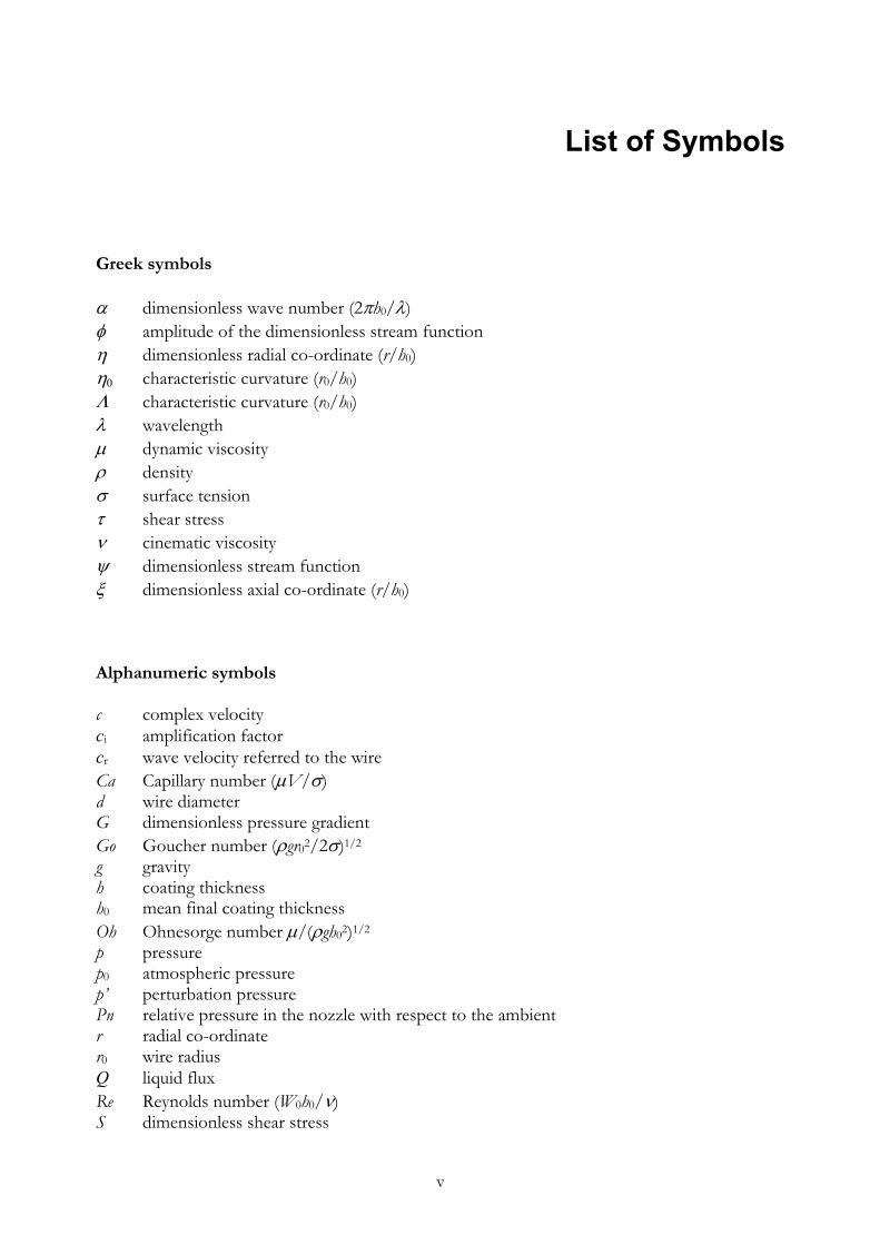
Greek symbols α dimensionless wave number (2πh0/λ) φ amplitude of the dimensionless stream function η dimensionless radial co-ordinate (r/h0) η0 characteristic curvature (r0/h0) Λ characteristic curvature (r0/h0) λ wavelength µ dynamic viscosity ρ density σ surface tension τ shear stress ν cinematic viscosity ψ dimensionless stream function ξ dimensionless axial co-ordinate (r/h0) Alphanumeric symbols c complex velocity ci amplification factor cr wave velocity referred to the wire Ca Capillary number (µV/σ) d wire diameter G dimensionless pressure gradient Go Goucher number (ρgr02/2σ)1/2 g gravity h coating thickness h0 mean final coating thickness Oh Ohnesorge number µ/(ρgh02)1/2 p pressure p0 atmospheric pressure p’ perturbation pressure Pn relative pressure in the nozzle with respect to the ambient r radial co-ordinate r0 wire radius Q liquid flux Re Reynolds number (W0h0/ν) S dimensionless shear stress
v
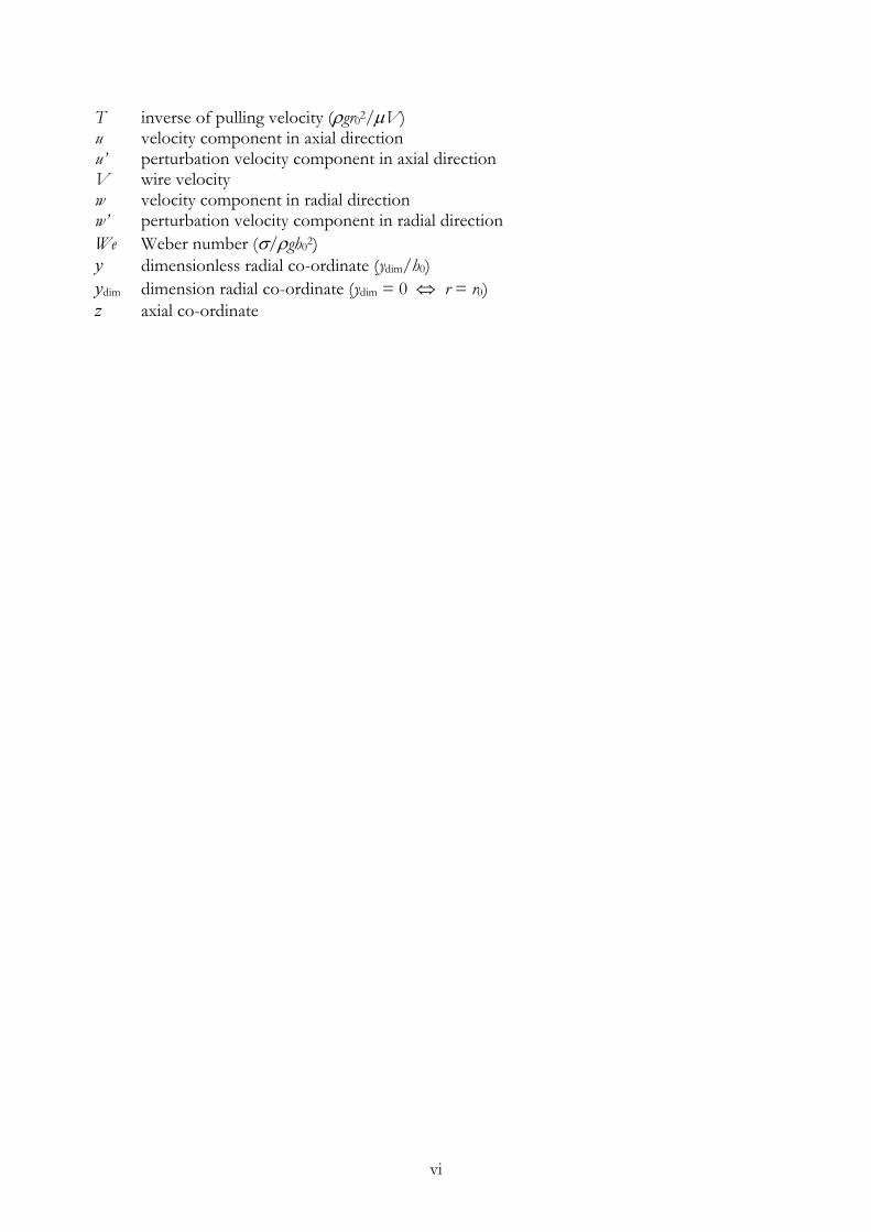
T inverse of pulling velocity (ρgr02/µV) u velocity component in axial direction u’ perturbation velocity component in axial direction V wire velocity w velocity component in radial direction w’ perturbation velocity component in radial direction We Weber number (σ/ρgh02) y dimensionless radial co-ordinate (ydim/h0) ydim dimension radial co-ordinate (ydim = 0 ⇔ r = r0) z axial co-ordinate
vi

List of Figures
Fig. 1.1: Instability observed in previous studies.................................................................................2 Fig. 1.2: Main coating techniques: simple withdrawal (a), die coating (b), jet wiping (c) ..............3 Fig. 2.1: Simple withdrawal ........................................................................................................................... 6 Fig. 2.2: Die coating ....................................................................................................................................... 8 Fig. 2.3: Die geometry ................................................................................................................................... 9 Fig. 2.4: Jet wiping coating.......................................................................................................................... 12 Fig. 3.1: Definition sketch ........................................................................................................................... 16 Fig. 3.2: Stability curves for We=100, V=0 and different r0 [8] ............................................................ 21 Fig. 3.3: Growth constant as function of wave number for simple withdrawal [9] ........................... 24 Fig. 3.4: Growth constant as function of wave number for die coating [9] ........................................ 24 Fig. 4.1: GALFIN facility - sketch ............................................................................................................. 32 Fig. 4.2: GALFIN facility – picture ........................................................................................................... 33 Fig. 4.3: Die for vertical die coating .......................................................................................................... 34 Fig. 4.4: Nozzle for jet wiping coating ...................................................................................................... 35 Fig. 4.5: Calibration for the CCD camera................................................................................................. 36 Fig. 4.6: Optical deformation ..................................................................................................................... 36 Fig. 4.7: CCD camera technique ................................................................................................................ 36 Fig. 4.8: Laser beam probe.......................................................................................................................... 37 Fig. 4.9: Laser beam technique................................................................................................................... 37 Fig. 4.10: Laser sheet technique.................................................................................................................. 38 Fig. 4.11: Laser sheet technique – wave speed measurement................................................................. 39 Fig. 4.12: Data processing procedure ........................................................................................................ 40 Fig. 4.13: Two signals measured at two different points ........................................................................ 42 Fig. 4.14: Two signals measured at two different points after shifting................................................. 42 Fig. 4.15: Position of the two probes ........................................................................................................ 43 Fig. 4.16: Typical power spectrum............................................................................................................. 44 Fig. 4.17: Filtering procedure...................................................................................................................... 44 Fig. 4.18: Example of filtering procedure ................................................................................................. 45 Fig. 6.1: Simple withdrawal – mean final thickness for laser sheet and laser beam probe ................ 52 Fig. 6.2: Simple withdrawal – mean final thickness for different distances from the bath ............... 53 Fig. 6.3: Simple withdrawal – mean final thickness compared with theory......................................... 53 Fig. 6.6: Simple withdrawal – wave velocity experimental and theoretical values .............................. 54 Fig. 6.7: Simple withdrawal – wave velocity experimental and theoretical in dimensionless form.. 55 Fig. 6.8: Simple withdrawal – typical power spectrum ........................................................................... 56 Fig. 6.9: Simple withdrawal – typical signal function of space (referred to figure (6.8)) ................... 56 Fig. 6.10: Simple withdrawal – measured wavelength compared with critical wavelength................ 57 Fig. 6.11: Simple withdrawal – measured wavelength compared with critical wavelength................ 58 Fig. 6.12: Simple withdrawal – measured wavelength compared with critical wavelength................ 59 Fig. 6.13: Simple withdrawal – wave amplitude at two different distances from the bath ................ 60 Fig. 6.14: Simple withdrawal – theoretical and experimental amplification factor ............................. 60
viii
ix
Fig. 7.1: Die coating – mean final thickness at different stations.......................................................... 63 Fig. 7.2: Die coating – theoretical wave velocity ..................................................................................... 64 Fig. 7.3: Die coating – relative wave amplitude ....................................................................................... 65 Fig. 7.4: Die coating – wavelength presence. V=0.122 m/s, Ca= 0.58, Go=0.483, T=0.76............ 66 Fig. 7.5: Die coating – wavelength absence. V≥0.297 m/s, Ca≤1.35, Go=0.58, T≤0.27 ................ 66 Fig. 7.6: Die coating – mean final thickness............................................................................................. 68 Fig. 7.7: Die coating – relative wavelength............................................................................................... 69 Fig. 7.8: Die coating – relative thickness .................................................................................................. 70 Fig. 7.9: Die coating – dimensionless wave velocity ............................................................................... 71 Fig. 7.10: Die coating – relative wavelength ............................................................................................. 72 Fig. 7.11: Die coating – power spectra for different Capillary number: a) Ca=1.59. b) Ca=2.57. c) Ca=3.57. d) Ca=3.77............................................................................................................. 73 Fig. 7.12: Die coating – relative wave amplitude ..................................................................................... 74 Fig. 7.13: Die coating – amplification factor ............................................................................................ 75 Fig. 7.14: Die with geometrical defects ..................................................................................................... 76 Fig. 7.15: Die with geometrical defect – reference figure....................................................................... 77 Fig. 7.16: Die with geometrical defect – case 1........................................................................................ 77 Fig. 7.17: Die with geometrical defect – case 1 – horizontal position.................................................. 78 Fig. 7.18: Die with geometrical defect – case 2........................................................................................ 79 Fig. 7.19: Die with geometrical defect – case 2 – horizontal position.................................................. 79 Fig. 7.20: Die with geometrical defect – case 3 ....................................................................................... 80 Fig. 7.21: Die with geometrical defect – case 4........................................................................................ 81 Fig. 8.1: Jet wiping coating – mean final thickness function of the wire velocity............................... 85 Fig. 8.2: Jet wiping coating – mean final thickness function of the stagnation pressure................... 86 Fig. 8.3: Jet wiping coating – mean final thickness: comparison between experimental data and “knife model” ........................................................................................................................ 87 Fig. 8.4: Jet wiping coating – mean final thickness: comparison between models ............................. 88 Fig. 8.5: Jet wiping coating – mean final thickness: comparison between models ............................. 89 Fig. 8.6: Jet wiping coating – mean final thickness: comparison at different stagnation pressure .. 91 Fig. 8.7: Jet wiping coating – mean final thickness: comparison at different Capillary number ..... 92 Fig. 8.8: Jet wiping coating – mean final thickness: comparison at two different distances from the nozzle ...................................................................................................................................... 93 Fig. 8.9: Jet wiping coating – wave velocity. L=92 mm, D=40 mm .................................................... 94 Fig. 8.10: Jet wiping coating – wave velocity. L=57 mm........................................................................ 95 Fig. 8.11: Jet wiping coating – wave velocity function of the stagnation pressure.............................. 96 Fig. 8.12: Jet wiping coating – wavelength Pn=0.5 kPa .......................................................................... 96 Fig. 8.13: Jet wiping coating – wavelength L=97 mm ............................................................................ 98 Fig. 8.14: Jet wiping coating – wavelength L=147 mm .......................................................................... 98 Fig. 8.15: Jet wiping coating – progressive disappearance of the observed wavelength. Ca=2.08. (a) Pn=0.5 kPa. (b) Pn=1 kPa. (c) Pn=3 kPa. ................................................................ 100 Fig. 8.16: Jet wiping coating – wavelength variation with the pressure.............................................. 101 Fig. 8.17: Jet wiping coating – wave amplitude, Pn=0.5 kPa............................................................... 102 Fig. 8.18: Jet wiping coating – wave amplitude, Pn=1 kPa .................................................................. 102 Fig. 8.19: Jet wiping coating – amplification factor, Pn=0.5 kPa........................................................ 103 Fig. 8.20: Jet wiping coating – relative wave amplitude: physical meaning........................................ 104 Fig. 8.21: Jet wiping coating – amplification factor, Pn=1 kPa ........................................................... 105 Fig. 8.22: Jet wiping coating – relative amplitude.................................................................................. 106 Fig. 8.23: Jet wiping coating – amplification factor............................................................................... 107 Fig. 8.24: Jet wiping coating – relaxation................................................................................................ 108

Chapter 1
Introduction 1.1 Introduction In the present work, the wire coating process will be investigated in details in order to understand the behaviour of the final liquid layer deposited on the wire. The main goal is the study of the instabilities encountered when a wire is covered by a liquid film since, if waves are present before drying, the final coating is not uniform. This is usually not desired for an industrial process: one reason is that if the wave amplitude is not negligible with respect to the mean thickness of the coating, the final finish is not good. Another reason is that the typical values of the coating characteristics can change for non-uniform coatings, like the heat transfer coefficient, important in chemical reactions. 1.2 Origin of the project In the previous years, some studies have been done at VKI concerning wire coating. Particular interest has been given to the annular jet wiping: the first model was introduced in 1996 by J. Anthoine [1] and then numerical studies [2] and further experimental investigations have been performed to validate the proposed models [3] [4]. Unfortunately, the simple “knife model” and the complete one have not yet been completely validated since discrepancies between predicted values and experimental results were found [3] [4]. In addition to this disagreement, the presence of instabilities was found during the experiments. A typical example of the instability observed is reported in figure (1.1)
1

50 100 150 200 250 300 350 400 450 500
50
100
150
200
250
Fig. 1.1: Waves observed in previous studies (in pixel) Starting from the conclusions given in the previous works, a detailed study of the instability behaviour will be the main goal of the present work, not limited to the jet wiping coating, but extended to different coating techniques encountered in the industry field. 1.3 Objectives of the project The main objective of this project is the study of the liquid film instabilities of wire coating. The behaviour of the liquid coating will be investigated for the main three different techniques sketched in figure (1.2). The first one, figure (1.2 - a) is the simple withdrawal in which the wire is drawn out from a liquid bath: the mean final thickness depend on the fluid properties and on the wire radius and velocity. The second one, figure (1.2 -b), is called die coating because the final thickness is reduced to the desired value using a mechanical device: the die. In this case the coating thickness is function of the geometry of the die, of the wire radius and of the fluid properties. The last technique considered is jet wiping coating, figure (1.2 -c). In this case the final thickness is reduced using an air jet in order not to have physical contact between the liquid and another object. The final coating thickness depends on the geometry of the nozzle,
2

Wire
h0
ρ, σ, µ
r0
V
NozzleJet
r0
h0 V
Wire
ρ, σ, µ
Die
r0
h0
V
Wire
ρ, σ, µ
(a) (b) (c) Fig. 1.2: Main coating techniques: simple withdrawal (a), die coating (b), jet wiping (c) on the pressure in the nozzle, on the wire radius, on the fluid properties and on the wire velocity. In all the cases the possible parameters that govern the process will be changed in order to understand their influence on the onset or on the offset of the instability. The most important characteristics that have to be measured to identify the stable or unstable behaviour of the fluid and that represents the main results expected by the experiments are: • mean final thickness • wave velocity • wavelength • amplitude • amplification factor Since up to now nothing has been developed at VKI concerning the study of instability for the wire coating, a literature search is needed in order to acquire the necessary background about the state of the art in this field. To reach the main goal, several sub-goals will be considered: • Literature search about instability of thin liquid films on wire and cylinders: something can
be found for the simple case without jet wiping. • Detailed experimental analyses for simple withdrawal coating, die coating and annular jet
wiping coating, changing for each case the parameters that influence the phenomenon, in order to check their influence on the final results.
• Validation of the previous theoretical models for the prediction of the final mean thickness, especially for the jet wiping case.
• Implementation and validation of the models found in literature for the prediction of the instability.
3
4
• Development and implementation of a theoretical model for the study of the instability in the jet wiping case.
• Validation of the new theoretical model developed.
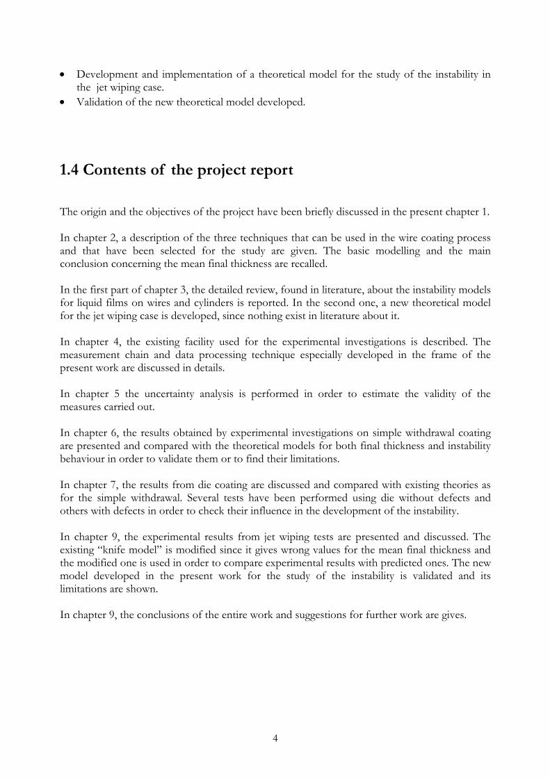
1.4 Contents of the project report The origin and the objectives of the project have been briefly discussed in the present chapter 1. In chapter 2, a description of the three techniques that can be used in the wire coating process and that have been selected for the study are given. The basic modelling and the main conclusion concerning the mean final thickness are recalled. In the first part of chapter 3, the detailed review, found in literature, about the instability models for liquid films on wires and cylinders is reported. In the second one, a new theoretical model for the jet wiping case is developed, since nothing exist in literature about it. In chapter 4, the existing facility used for the experimental investigations is described. The measurement chain and data processing technique especially developed in the frame of the present work are discussed in details. In chapter 5 the uncertainty analysis is performed in order to estimate the validity of the measures carried out. In chapter 6, the results obtained by experimental investigations on simple withdrawal coating are presented and compared with the theoretical models for both final thickness and instability behaviour in order to validate them or to find their limitations. In chapter 7, the results from die coating are discussed and compared with existing theories as for the simple withdrawal. Several tests have been performed using die without defects and others with defects in order to check their influence in the development of the instability. In chapter 9, the experimental results from jet wiping tests are presented and discussed. The existing “knife model” is modified since it gives wrong values for the mean final thickness and the modified one is used in order to compare experimental results with predicted ones. The new model developed in the present work for the study of the instability is validated and its limitations are shown. In chapter 9, the conclusions of the entire work and suggestions for further work are gives.

Chapter 2
Wire Coating Process 2.1 Introduction The application of liquid coating to substrates is a process encountered in many industries. Typical examples are the coating of paper or metal sheets with decorative or protective materials and the application of adhesives to films and tapes [5] [6] [7]. Wire coating is an industrial process in which a wire is drawn out from a liquid bath in order to cover the surface of the wire with a thin film of liquid. This layer, after drying becomes the coating. Since this is an industrial process, high productivity and the possibility to control the final thickness are required. Usually, if the velocity of the wire is increased, the thickness of the coating increases so that different techniques have been developed and can be applied in order to obtain the desired final coating thickness: simple withdrawal, die coating and jet wiping. In the following paragraphs they’ll be described more in details. It’s important to keep in mind that in the present chapter only the basic flow is solved for each kind of coating process. 2.2 Simple withdrawal Simple withdrawal is the simplest technique in wire coating. The wire is drawn out from the liquid bath and it is dried without undergoing any other kind of treatment. In (fig. 2.1) the basic scheme is shown: the wire is driven inside the bath by a whirl and drawn out with a velocity V.
5
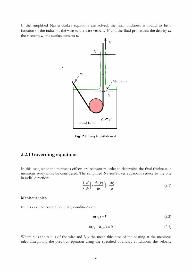
If the simplified Navier-Stokes equations are solved, the final thickness is found to be a function of the radius of the wire r0, the wire velocity V and the fluid properties: the density ρ, the viscosity µ, the surface tension σ.
Meniscus
Liquid bath
Wire
h0
ρ, σ, µ
r0
V Fig. 2.1: Simple withdrawal 2.2.1 Governing equations In this case, since the meniscus effects are relevant in order to determine the final thickness, a meniscus study must be considered. The simplified Navier-Stokes equations reduce to the one in radial direction:
µρg
drrdur
drd
r=
)(1 (2.1)
Meniscus inlet. In this case the correct boundary conditions are:
Vru =)( 0 (2.2)
0)( 00 =+ INhru (2.3) Where r0 is the radius of the wire and h0IN the mean thickness of the coating at the meniscus inlet. Integrating the previous equation using the specified boundary conditions, the velocity
6

profile can be obtained and from it the liquid flux. Adding the boundary condition for the pure dragging model
0)( 00 =
+drhrdu IN (2.4)
it is possible to obtain the final thickness solving the implicit equation [3]:
( ) ( )
−+−
++=
+ 0
20
200
0
0000
00
ln24 r
rhrrhrhrg
hrV ININ
ININ µ
ρ (2.5)
and using the previous thickness the liquid flux ( )INhQ 0 can be computed. Detailed description is found in [3]. Meniscus outlet. In this case the correct boundary conditions are:
Vru =)( 0 (2.6)
kVhru =+ )( 00 (2.7) where h0 is the mean thickness of coating after the meniscus and k a constant to be determined. Repeating the same procedure as for the meniscus inlet, and applying the further boundary condition
0)( 00 =
+drhrdu (2.8)
the following equation is derived in order to obtain the final thickness h0 :
( ) ( ) ( )
−+−
++=
+−
0
20
200
0
0000
00
ln24
1r
rhrrhrhrg
hrkV
INµρ (2.9)
the liquid flux Q can be computed knowing h( 0h ) 0 . Solution Since the continuity has to be satisfied, a constraint is given by:
( ) ( )00 hQh INQ = (2.10) Solving the system (2.9)-(2.10) the value of the constant k and of the final thickness h0 can be obtained. For more details, see [3] [4].
7

2.3 Die coating Since wire coating is an industrial process, it is be better to have a well-defined coating thickness independent on the velocity: in this way high productivity can be easily achieved. This goal can be reached using a die: it is a small orifice, through which the wire passes and from which it is extruded. The main problem is that there is physical contact between the liquid and the die and in many cases this technique cannot be used (galvanisation for example). A sketch of the die coating process is shown in (fig. 2.2).
DieR1
R2
r0
h0
V
MeniscusWire
Liquid bathρ, σ, µ
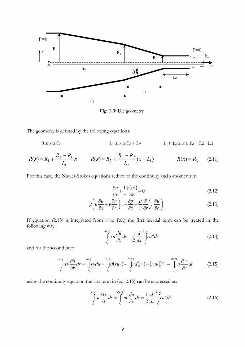
Fig. 2.2: Die coating The final thickness depends on the properties of the fluid, on the radius of the wire and on the geometry of the die. 2.3.1 Governing equations A simple theory exists for the horizontal die coating, taking into account the geometry of the die. Since the horizontal configuration is considered, the gravity effect is neglected. The sketch is shown in (fig. 2.3)
8
ϑ
R3
R2R 1
r o
L 3
x
r h0
L2
P=0
P=0
V
L 1
Fig. 2.3: Die geometry The geometry is defined by the following equations:
0 ≤ x ≤ L1 L1 ≤ x ≤ L1+ L2 L1+ L2 ≤ x ≤ L1+ L2+L3
xLRR
RxR1
121)(
−+= )()( 1
2
232 Lx
LRR
Rx −R−
+= (2.11) 3)( RxR =
For this case, the Navier-Stokes equations reduce to the continuity and x-momentum:
( ) 01=
∂∂
+∂∂
rrv
rxu (2.12)
∂∂
∂∂
+∂∂
−=
∂∂
+∂∂
rur
rrxp
ruv
xuu µρ (2.13)
If equation (2.13) is integrated from ro to R(x) the first inertial term can be treated in the following way:
∫∫ =)(
2)(
21 xR
r
xR
r oo
drrudxddr
xuru∂∂ (2.14)
and for the second one:
( ) ( ) [ ] ∫∫∫∫∫ −=−==)(
)()()()()( xR
r
xRr
xR
r
xR
r
xR
r
xR
r o
o
oooo
drrrvuruvrvudruvdrvdudr
rurv
∂∂
∂∂ (2.15)
using the continuity equation the last term in (eq. 2.15) can be expressed as:
∫∫ ==−)( )(
2)(
21xR
r
xR
r
xR
r o oo
drrudxddr
xuurdr
rrvu
∂∂
∂∂
∫ (2.16)
9
Finally, the integral form of the momentum equation becomes:
∫
−
+
−−=
)( 222
2
xR
r ro
R
o
o orur
ruR
dxdprRdrru
dxd
∂∂µ
∂∂µρ (2.17)
It’s now necessary to introduce a velocity profile in order to solve the previous equation. The simplest is a parabolic one:
21 ηη baVu
++= (2.18)
where
)(xhrr o−
=η (2.19)
and 0)()( rxRxh −= (2.20)
For determining the two coefficients a and b, two relations are required. The first one is the no-slip condition at r = R(x) where η = 1:
0 1= + +a b (2.21) the second one can be derived from equation (2.17), by the hypothesis of negligible inertia. Generally:
( )∂∂
∂∂η
ηη
ur
u ddr
Uh x
a b= = ⋅ +( )
2 (2.22)
Using equation (2.22), equation (2.17) becomes
[ ][ ]dxdprR
arbaRxhV o
o 22
)(
22 −=−+
µ (2.23)
A normalised pressure gradient can be introduced in order to simplify the form of equation (2.23):
dxdp
Vxhp
µ)('~
2
= (2.24)
The linear system for a and b is finally obtained:
+
−=⋅
+ '~
21
1
142
11
phr
ba
hr oo (2.25)
10
and the solution is:
++
+−=2'~
21
11 p
hr
ao
++
=2'~
21
1 p
hr
bo
(2.26)
The flow rate is given by the expression:
( )(∫∫ +++==1
0
2122 ηηηηππ dbahrVhurdrQ o
R
ro
) (2.27)
Integrating one obtains:
ooo rhbrharh
VhQ
++
++
+=
234232π (2.28)
If the expressions (2.26) of a and b are injected in the relation (2.28) the differential equation for the pressure gradient is obtained:
[ ][ ])()()(
)()()()()(1)(21
2 xCxDxhxExDxAxCxAxB
dxdp
V −−−++
=µ
(2.29)
where:
)(2
1
1)(
xhr
xAo+
= ;)(
)( 0
xhrhxB o= ;
23)()( orxhxC += ;
34)()( orxhxD += ; or
xhxE +=2)()( (2.30)
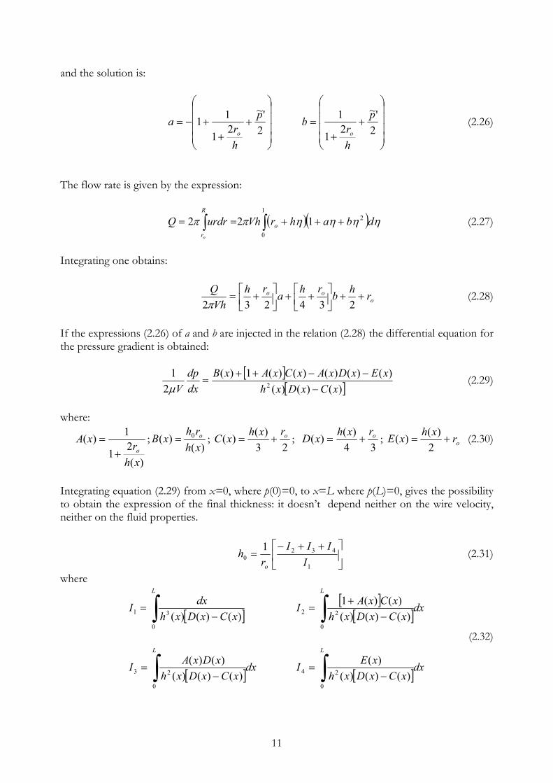
Integrating equation (2.29) from x=0, where p(0)=0, to x=L where p(L)=0, gives the possibility to obtain the expression of the final thickness: it doesn’t depend neither on the wire velocity, neither on the fluid properties.
++−=
1
4320
1I
IIIro
h (2.31)
where
[ ]∫ −=
L
xCxDxhdxI
0
31 )()()( [ ]
[ ]dxxCxDxhxCxAI
L
∫ −+
=
0
22 )()()()()(1
(2.32)
[ ]dxxCxDxhxDxAI
L
∫ −=
0
23 )()()()()( [ ]dxxCxDxh
xEIL
∫ −=
0
24 )()()()(
11

2.4 Annular jet wiping coating In this kind of coating process, the final thickness is controlled by an annular jet impinging on the wire covered by the liquid film. The jet produces a reduction of thickness depending on different parameters like the geometrical characteristic of the nozzle, the radius of the wire, the fluid properties and the pressure in the nozzle. Since in this case there is no contact between the coating and the device used in order to reduce the thickness, annular jet wiping can be used for galvanisation and all the times the physical contact must be avoided.
Nozzle
R1 jet
r0
h0
V
MeniscusRun-back flow
Wire
Liquid bathρ, σ, µ
Fig. 2.4: Jet wiping coating 2.4.1 Governing equations Simplifying the Navier-Stokes equations, considering the flow stationary, incompressible and the inertia negligible, the following equation is obtained, in which the viscous shear stress balances the gravity, the pressure and the tension term:
( )3
3 )()(,dxxhdg
dxxdp
rrxur
rrσρµ
−+−=
∂∂
∂∂ (2.33)
where p(x) is the relative pressure profile provided by the jet and x the axial co-ordinate and r the radial one.
12

The boundary conditions for the previous equations are:
Vru =)( 0 (2.34)
( )xr
xhrxujetτµ =
∂+∂ ))(,( 0 (2.35)
where V is the velocity of the wire and τjet the shear stress profile provided by the jet. Integrating equation (2.33) with boundary conditions (2.34)-(2.35) the liquid velocity profile
is obtained: ),( rxu
( ) ( ) ( )
+⋅−++−+=
000
20
2 ln)(2
)(4 r
rxhrABxhrrrAVu (2.36)
where
( )
−+= 3
3 )()(1dxxhdg
dxxdpxA σρ
µ (2.37)
( )µ
τ xxB jet=)( (2.38)
The liquid flux can be computed by:
∫+
=)(0
0
),(2xhr
rdrrxruQ π (2.39)
For the velocity profile given by (2.36) it becomes:
( )( ) ( )( ) ( )
−
++++−++−+= 1
)(ln2
4)(
4)(
16)(
22
0
02
02022
02
022
0 rxhrxhrr
CrxhrARxhrVQ π
(2.40) where:
( ) ( )
+⋅−+= )(
2)()()()( 00 xhrxAxBxhrxC (2.41)
The conclusion is that if the pressure gradient and the shear stress profile due to the jet are known, the shape of the final thickness h(x) can be computed from equation (2.40): this is called the complete model. If the previous profiles are not known, it is possible to assume that all the forces are located in only one point (the knife point): only the maximum value of the pressure gradient and shear
13

stress due to the jet are taken into account instead of all the profiles. This is called “knife model” and applying the condition
0=dhdQ (2.42)
the knife thickness is given by:
( ) ( ) ( )( )+−+⋅+⋅++ 20
2000 2
rhrhrAhrV kkk
( ) ( ) ( ) ( )0ln
61ln6
403
002
020 =
++−
−
+++
Rhr
hrARhr
hrrB kk
kk
(2.43)
where the functions A and B are computed for the maximum value of the pressure gradient and shear stress. Once the knife thickness hk has been computed, it is possible to evaluate the liquid flux Qk from equation (2.40) and from Qk the final thickness hfinal after the jet:
( )( )2020 rhrVQ finalk −+= π (2.44)
The “knife model” is very simple and can be easily applied since it doesn’t require the complete pressure and shear stress profiles. On the other hand, a correlation between the maximum of them that have to be used is needed. From previous works [1], the following expression are proposed:
ZsPn
dxdp
MAX
210= (2.45)
and
366.0
2
22.0
=
sUU
jet
airjetairMAXjet
υρτ (2.46)
where Pn is the stagnation pressure in the nozzle, s the slot size of the nozzle, ρair and υair the density and kinematic viscosity of the air, Ujet the jet velocity computed by the nozzle pressure and Z is given by
2dDZ −
= (2.47)
with D being the internal diameter of the nozzle and d the diameter of the wire. For more details on annular jet wiping and the “knife model”, see [1] [2] [3] [4].
14

Chapter 3
Wire Coating Instabilities 3.1 Introduction In wire coating process, a smooth and uniform layer of liquid is required, but sometimes it is difficult to achieve it because of flow instabilities. The instability, frequently, sets a limit on the production rate or dictates the selection of the material in precision coating. A predictive theory of film instability is therefore of considerable practical significance. The standard procedure in developing a stability theory is: • to compute the basic flow from the simplified Navier-Stokes equations and appropriate
boundary conditions (see chapter 2), • to add a small disturbance to the basic flow and to inject the new flow field into the Navier-
Stokes equation, neglecting higher order terms of the perturbation quantities, • to introduce a stream function in order to satisfy automatically the continuity equation for
the perturbation velocities, • to rewrite the Navier-Stokes equations in dimensionless parameters, condensing the
continuity and momentum equations in only one equation for the stream function, plus boundary conditions,
• to introduce an asymptotic expansion for the stream function based an a small parameter • to express the shape of the wave as an amplitude multiplied by an exponential, • to check if the wave is amplified or not (instability or not), looking at the imaginary part of
the complex eigenvalue. In the following paragraphs, a description of the instability theory will be given.
15

3.2 Problem formulation Consider the flow of a viscous incompressible fluid down a wire (or a cylinder) as sketched in figure (3.1). At this stage, it is not important to know if the flow comes from a simple withdrawal process, a die coating or annular jet wiping because the flow far from the bath or from the device used to reduce the final thickness is dominated always by the same equations. In this paragraphs, the theory developed by Lin & Liu is presented [8]. The Navier-Stokes equations, since the fluid is incompressible, are:
0=⋅∇ V (3.1)
( ) gVPVVtV
+∇+∇−=⋅∇+∂∂ 21 υ
ρ (3.2)
where ∇ is the gradient operator and the Laplacian. 2∇
Fig. 3.1: Definition sketch
16

3.2.1 Basic flow If the Navier-Stokes equations are simplified, with the hypothesis of parallel flow in the axial direction, the simple following equation is derived:
0=+
∂∂
∂∂ g
rVr
rrzν (3.3)
where υ is the kinematic viscosity and Vz is the velocity in the axial direction, function of the radial co-ordinate. The boundary conditions for equation (3.3) are the no-slip condition at the wall and the vanishing net force at fluid-air interface:
VrVz =)( 0 (3.4)
0)( 00 =
∂+∂rhrVz (3.5)
where r0 is the radius of the wire and h0 the mean final thickness of the coating. Integrating equation (3.3) using boundary conditions (3.4)-(3.5), the velocity profile in z direction, function of the radial position, can be obtained:
( ) ( )
++−=
0
200
220 ln
24)(
rrhrgrrgrVz υυ
(3.6)
For the pressure, the relationship is:
0pp = (3.7) which means that the pressure is constant and equal to the atmospheric pressure. 3.2.2 Perturbations Once the basic flow has been obtained, a perturbation is introduced in order to check if it grows up or if it is damped down:
vrViV zz += )(ˆ (3.8)
ppP += (3.9)
17

where is the unit vector in the direction of g and zi v and p are respectively the velocity and pressure perturbations. Substituting expressions (3.8)-(3.9) into equations (3.1) and (3.2), and writing the resulting equations in cylindrical co-ordinates ( zr ,, )θ , one obtains:
0=∂∂
++∂∂
zw
ru
ru (3.10)
( )
∂∂
+∂∂
−∂∂
+∂∂
−=∂∂
++∂∂
+∂∂
2
2
2
2 11zu
ru
rru
rp
zuwV
ruu
tu
z υρ
(3.11)
( ) ( )
∂∂
+
∂∂
∂∂
+∂∂
−=∂
+∂+
∂∂
++∂∂
2
211zV
rwr
rrzp
rwVu
zwwV
tw zz
z υρ
(3.12)
where are the (( wvu ,, ) )zr ,,θ component of the disturbance velocity field. In arriving at equations (3.10)-(3.12), the disturbance is assumed to be axisymmetric, that is, v is taken to be zero. The boundary conditions for the disturbances are the no-slip condition on the wire and the vanishing of the total tangential and normal force per unit area at the liquid-air interface:
0)()( 00 == rwru (3.13)
0))(( 0 =+ zhrpt (3.14)
011))((21
00 =
+−++RR
zhrpp n σ (3.15)
where
21
21
1
11
∂∂
+
−=
zhr
R and
23
2
2
2
2
1
1
∂∂
+
∂∂
=
zh
zh
R (3.15)
are the curvature of the free surface and pt and pn are, respectively the tangential and normal force exerted by the fluid on each unit area of the free surface. In addition, the following kinematic condition must be satisfied at the free surface:
( )zhwV
thu z ∂
∂++
∂∂
= (3.16)
18

3.2.3 Dimensionless variables It is possible to introduce dimensionless variables as following:
lz
=ξ ; 0hr
=η ; 0hhd = ;
ltW0=τ ;
00Whul
=′u ; 0WwVw zW +
=′+ ; 0ghpppp
ρ+
=′+′ (3.17)
where l is a characteristic length in the axial direction and W0 is the maximum velocity at the interface liquid-air (see fig. (3.1)). Introducing a stream function ψ related to the velocity perturbations by
ηψ
η ∂∂
=′ 1w and ξψ
η ∂∂
−=′ 1u (3.18)
and combining equations (3.10)-(3.12) the following equation for the stream function is obtained:
++−−−=−+− ηηξηξηηξτητηηηηηηηηηηηη ψ
ηψψ
ηψ
ηψ
ηψ
ηαψ
ηψ
ηψ
ηψ
ηWW
322432
111Re3321
+
−+
−−−−+ ηηξξηξξηηηηηηηη
ηξηηξη ψ
ηψ
ηαψ
ηψ
ηψ
ηηψ
ηψψ
η11213311
22
2232 WW
ξξξξξηξξξξξξξξητξξ ψαψψη
ψψη
ψψη
ψα 42
3 121Re −
−+
++ W (3.19)
where lh0=α is the dimensionless wave number if l is taken to be πλ 2/ and λ is the
wavelength, and υ
00hW=Re the Reynolds number.
Of course, also the boundary conditions (3.13)-(3.15) have to be rewritten as function of ψ : they will not be presented here since all the details can be found in reference [8]. 3.2.4 Solutions It is now necessary to solve the equation (3.19). According to observations, the film instability exhibits itself a gravity capillary waves so long that 10 <<= lhα where. Therefore it is possible to expand the solution of equation (3.19) in powers of the small parameter α.
( )∑=
=0n
nnψαψ (3.20)
19

The stream functions ( ) are determined by solving equation (3.19) plus boundary conditions with the method of regular perturbation, which means that the function ψ is written as
nψ
( ) ( ) )2(10 ααψψψ O++= and injected in equation (3.19) and relative boundary conditions. The different terms at zero order and first order are then grouped and from the zero order equation and boundary conditions ψ(0) is found, while from the first order set of equations ψ(1) is obtained. Substituting the solution obtained into the kinematic condition gives a single non-linear partial differential equation that governs the motion of the free surface. In can be linearized noticing that during the initial stage of the instability the wave amplitude is small, so that we can write:
εζ+=1d ; 1<<ε (3.21) substituting (3.21) in the non-linear partial differential equation for the free surface, neglecting the terms smaller than ( )εO , and applying the Gallilei transformation τξ VZ += , one obtains:
( )( ) ( ) ( )( ) ( )( ) 0111Re1 0 =+++−+ zzzzz DWeCBVA ζζαζζ ξξτ (3.22) where V is the dimensionless wire velocity and the other functions are defined as: 00 /WV=
( )
+−=
0
2220 ln2
ηη qqqdA (3.23)
( ) ( ) ( )( ) ( ) +−+−+−=16ln717
8ln5ln
21 2
022
02
222
0436 QqqQqqQqdB ηηη
40
220
460
6
649
6415
19216
19259 ηηη qqq −−+ (3.24)
( )
−
−
+=
0
2
0
4
0 ln4438 η
ηη qqq
qdC (3.25)
( ) ( )WedMdD 22α−= (3.26)
( )16ln
416163 32
0303 QqqQqdM +−+=
ηη (3.27)
where
dq += 0η (3.28)
dQ
+=
0
0
ηη (3.29)
0
00 h
r=η (3.30)
and 20gh
Weρ
σ= is the Weber number, the inverse of the better known Bond number,
σρ 2
0ghBo = .
20

Equation (3.22) admits the normal mode solution
( )[ ]τδζ cZi −= exp (3.31) where δ is the wave amplitude which is indeterminate in the framework of linear theory and
is the complex eigenvalue given by: ircc = ic+
0)1( VAcr −= (3.32)
( ) ( ) ( )( )( )21211Re αα MCWeBci −+= (3.33) Developing the equations c is found at the zero order while at the first order. r ic 3.2.5 Physical interpretation In physical terms, is the absolute wave speed and c is the exponential growth rate or damping rate of the disturbance depending on the condition c or
rc i
i 0> 0<ic .
α
Fig. 3.2: Stability curves for We=100, V=0 and different r0 [8] The stability curves are plotted in figure (3.2) for three different values of 0η . The film is stable in the region above each neutral curve ( 0=ic ), since 0<ic there, while the film is unstable in
21

the regions of Re−α plane where c . A few curves of constant damping and amplification rate are also given in the same figure (3.2). It is seen that each neutral curve intersects the vertical axes at a cut-off wave number
0>i
Cα that can be easily obtained from equation (3.33) for : 0Re ==ic
0η
( )1 2
/1/ R 2/ R
1R
) 21α2WeM−
((C
11
0 +=
ηαC (3.34)
This means that any disturbance whose wave number is smaller than the cut-off wave number will make the flow unstable for all the values of Re. Moreover, from figure (3.2) it is clear that the film becomes unstable with respect to the disturbance of a given wave number at a smaller Re as , the ratio between the wire radius and the film thickness, decreases. The physical reason is inside equation (3.33): it can be shown that ( ) 01 >C and ( ) 01 >M , thus the term WeC and ( )12 αWeM
2/ R
− represent, respectively, destabilising and stabilising effects. From the detailed analysis [8] it can be shown that they arise respectively from the curvature terms T and T .1 is the free surface curvature associated to the surface displacement variation in the axial direction, and 1 is the curvature measured along a surface curve orthogonal to the wave profile. Therefore, the term WeC represents capillary pinching which destabilises the film and the term
( )1( represents the capillary elasticity that opposes the surface wave formation.
It can be further noted that the sum ) ( ) )2121 αM−We in equation (3.33) is positive if Cαα < . This implies that, in this case, the wavelength is so long that the capillary elasticity is entirely dominated by the capillary pinching which is independent of the wavelength, and thus the film is unstable no matter how small the destabilising inertial effect represented by Re is. On the other hand, the same sum is negative if Cαα > . This implies that if the wavelength is sufficiently small, then the capillary elasticity dominates over the capillary pinching and the film may be stable if Re is sufficiently small. 3.3 Dimensionless parameters Different dimensionless groups can be considered in the stability of coatings on wires. Some of them have already been introduced: The inverse of the dimensionless curvature
0
00 h
r=η (3.35)
Reynolds number, the ratio between the inertial and viscous forces
υ00Re hW
= (3.36)
22
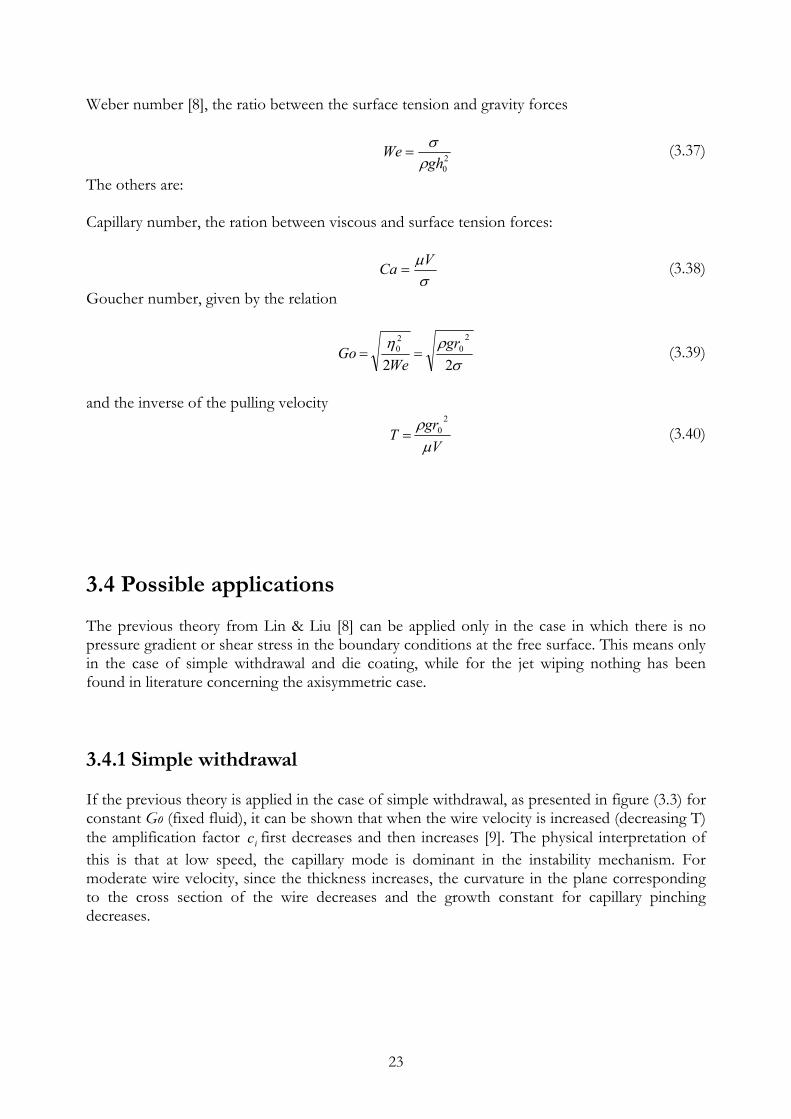
Weber number [8], the ratio between the surface tension and gravity forces
20gh
Weρ
σ= (3.37)
The others are: Capillary number, the ration between viscous and surface tension forces:
σµVCa = (3.38)
Goucher number, given by the relation
σρη22
20
20 grWe
Go == (3.39)
and the inverse of the pulling velocity
Vgr
Tµ
ρ 20= (3.40)
3.4 Possible applications The previous theory from Lin & Liu [8] can be applied only in the case in which there is no pressure gradient or shear stress in the boundary conditions at the free surface. This means only in the case of simple withdrawal and die coating, while for the jet wiping nothing has been found in literature concerning the axisymmetric case.
3.4.1 Simple withdrawal If the previous theory is applied in the case of simple withdrawal, as presented in figure (3.3) for constant Go (fixed fluid), it can be shown that when the wire velocity is increased (decreasing T) the amplification factor first decreases and then increases [9]. The physical interpretation of this is that at low speed, the capillary mode is dominant in the instability mechanism. For moderate wire velocity, since the thickness increases, the curvature in the plane corresponding to the cross section of the wire decreases and the growth constant for capillary pinching decreases.
ic
23

8.33⋅10
5⋅10-
2 5⋅100
20
40
60
0 0.01 0.02 0.03 0.04
T=8.33·10-5
T=2.5·10-4T=5·10-4
α
ci
Go=1.58·10-2 Fig. 3.3: Growth constant as function of wave number for simple withdrawal [9] 3.3.2 Die coating Applying the Lin & Liu theory to the die coating process as done by Homsy & Geyling [9], we find that at fixed thickness and varying the wire speed, the growth constant decreases with increasing speed and that the wave number of maximum growth remains approximately constant. The decrease of the growth constant with increasing speed for fixed thickness can be understood by noting that as T goes to zero, the velocity profile becomes more like a plug flow, eliminating the long surface wave which relies on the base flow shear for its energy [9]. Characteristic curves are shown in figure (3.4) and the behaviour for decreasing T is clear.
8.33T=8.33·10-5⋅10
5⋅10T=5·10-5 -
2 5⋅T=2.5·10-4100
0.5
1
1.5
2
0 0.05 0.1
T=1.25·10-4
α
ci
Go=1.58·10-2 Fig. 3.4: Growth constant as function of wave number for die coating [9] 3.3.3 Annular jet wiping For the annular jet wiping nothing exists in literature. If one is not interested in what happens in the region of the jet, and wants only to concentrate the attention on the flow far from the impinging region, the previous theory can be applied without any modification.
24
3.5 Development of the theoretical model for jet wiping instability
The theory developed by Lin & Liu can be applied only for the case of simple withdrawal and die coating, as presented in the previous paragraphs. For the annular jet wiping, the model needs to be extended to the case in which a pressure gradient and a shear stress profile are present at the free surface. It is important to underline the fact that in literature nothing has been found concerning the instability of an axisymmetric flow having a pressure gradient and a shear stress profile as boundary conditions at the liquid-air interface. For this reason a new theory is developed in this project in order to predict the instability behaviour in the case of jet wiping coating. The only works about jet wiping instabilities found in literature are for the planar case [10] [11], in which a 2D planar Newtonian flow is considered. The boundary conditions provided at the free surface are a pressure distribution and a shear stress profile. The steps followed by Tu & Ellen [11] are the standard ones, as seen in the presentation of Lin & Liu theory [8]. They can be summarised as: • Solution of the basic flow with the appropriate boundary conditions at the free surface
(pressure distribution and shear stress profile) • Introduction of the perturbations and linearization of the Navier-Stokes equations around
the basic flow • Introduction of the stream function in order to rewrite the continuity and momentum
equations as only one equation for ψ • Asymptotic expansion of the solution ψ and the complex eigenvalue c as power of the wave
number supposed small The system of differential equations obtained from the previous considerations is than solved and the wave velocity cr and the amplification factor ci are found. Starting from the works about 2D jet wiping instabilities found in literature [10] [11] and from the instability of thin liquid films on wire and cylinders [8] [9] [12], a new theoretical model is developed for the anular jet wiping. The complication with respect to the planar case is given by the introduction of the axisymmetric co-ordinates that produce the raising of a logarithmic term, while the complication with respect to the axisymmetric case without jet is due to the introduction of a the pressure profile and shear stress at the free surface. Instead of following the steps found in [8], the theoretical development will follow the ones used by Krantz and Zollars [12] since in this case the calculation of the stream function at the first order is not needed.
25

3.5.1 Basic flow The previous works developed at VKI [1] [2] [3] [4] gives the basic flow for the annular jet wiping. Rewriting equation (2.36) in dimensionless form and neglecting the surface tension term, since it was found that its influence is not so strong [3], the following expression for the dimensionless velocity profile of the basic flow is found:
( ) ( )[ ] ( )
+Λ−
Λ+Λ
−+Λ+Λ= 22ln2112)( yyGySGyu η (3.41)
where: • is the dimensionless radial co-ordinate chosen so that y=0 defines the surface of the wire.
This co-ordinate plays the role of r in the Lin & Liu theory: the difference is that the origin is shifted
y
0
dim
hy
y = (3.42)
• G is the dimensionless pressure gradient term given by:
dxdp
gG
ρ11+= (3.42)
• S is the dimensionless shear stress term given by:
0ghS jet
ρτ
= (3.43)
• Λ is the curvature group corresponding to 0η :
0
0
hr
=Λ (3.44)
• η is the dimensionless velocity at the free surface ( 1=y ):
( ) ( )[ ] ( )2121ln2112
1
+Λ−
Λ+Λ
−+Λ+Λ=
GSGη (3.45)
26

3.5.2 Orr-Sommerfeld equation Once the basic flow has been obtained, it can be injected in the Orr-Sommerfeld equation derived for the axisymmetric case and the relative 4 boundary conditions. Since this part is well described in [12], we refer to the reference for the complete equation and boundary conditions. The solution of the problem is found expanding the stream function as power of the dimensionless wave number α:
)( 210 ααφφφ O++= (3.46)
and the complex wave velocity in the same way:
)( 210 αα Occc ++= (3.47)
If expressions (3.46) and (3.47) are inserted in the dimensionless Orr-Sommerfeld equation [12] 0φ and 1φ have to satisfy the respectively the zeroth and first order equations and boundary
conditions obtained grouping the terms and . 0α 1αOnce 0φ and 1φ have been obtained from the system of equations at zeroth and first order, the solution is given by (3.46). 3.5.3 Solution at zeroth order At zeroth order, the Orr-Sommerfeld equation is:
( ) ( )0'3''3'''2'''' 030200 =
+Λ−
+Λ+
+Λ− φφφφ
yyy (3.48)
with boundary conditions:
0'0 =φ @ (3.49) 0=y
00 =φ @ (3.50) 0=y
0Re
Re4'1
2'' 00
200 =−
++Λ
− − φηφφcOh
@ (3.51) 1=y
( )
0'11''
11''' 0200 =
+Λ+
+Λ− φφφ @ (3.52) 1=y
where Re is the Reynolds number based on the velocity at the free surface and Oh the Ohnesorge number given by:
27

0hOh
ρσµ
= (3.53)
Integrating equation (3.48) the homogeneous integral is found with 4 unknown. They can be obtained by injection the solution in the four boundary conditions (3.49) – (3.52): a linear system 4 by 4 is obtained. Since the problem is homogeneous, the matrix must be singular: this condition can be satisfied since a degree of freedom has not yet been used, c . Imposing the determinant of the matrix equal to zero, the following solution is found:
0
( )
+
−Λ−
Λ+Λ
+Λ+Λ= 1121ln242Re 220 ηOhc (3.54)
The previous expression is referred to the wire frame, so that the absolute wave velocity is V-c0. The pressure gradient and the shear stress profiles enter in the expression (3.54) by η . Expression (3.54) reduces to the one found by Krantz & Zolars [12] in the case of G=1 and S=0, which is the same found by Lin & Liu [8]. 3.5.4 Solution at first order At first order, the Orr-Sommerfeld equation is:
( ) ( )=
+Λ−
+Λ+
+Λ− '3''3'''2'''' 131211 φφφφ
yyy
( )( ) ( ) ( )
+Λ
−−
+Λ
−− −00000
2 ''''Re'1''Re φφφφyyuyu
ycOhyui (3.48)
with boundary conditions:
0'1 =φ @ 0=y (3.49)
01 =φ @ 0=y (3.50)
( ) 020
21
2
10
211Re
Re4Re
Re4'1
1'' φη
φηφφcOh
cOhcOh −
−
−−
−=−
++Λ
− @ (3.51) 1=y
( )=
+Λ+
+Λ− '
11''
11''' 1211 φφφ
( )( )
+Λ−
−−− −
−−
022
02
2
002
11
Re'Re φαφ
cOhOhcOhi @ (3.52) 1=y
Again, the general integral of equation (3.48) contains four integral constants to be determined. The system obtained by the four boundary conditions is no more homogeneous, but the
28

coefficient matrix is singular since the homogeneous part of the problem is the same found at zeroth order. This means that another condition has to be used in order to guarantee the solvability of the system and the degree of freedom is given by c . This condition is found from the following considerations: since the determinant of the coefficient matrix of the system is singular, it means that one of the rows of the matrix is a linear combination of the other. For example, the fourth row can be expressed as a linear combination of the previous. The condition is obtained imposing the known term of the fourth equation equal to the same linear combination of the rows of the matrix. An equation is obtained and the only parameter that can be fixed in order to satisfy it is .
1
1c Applying this technique, the following expression for has been found: 1c
( )
+Λ−+
= 2
22221 1
12Re81 αη fOhfc (3.54)
where
f1DEN
(3.55) NUM1 NUM2.NUM1 NUM2
with the following expressions for NUM1, NUM2, DEN, where LOG stands for
LOG ln Λ 1Λ
(3.56)
DEN Λ 1( ) 16 Λ
7. ln Λ( ). LOG2. 32 87 Λ3. 191 Λ
2. 118 Λ. 64 Λ8. LOG2. 64 Λ.. _ 6
6
90 Λ4. 16 ln Λ( ). Λ
5. 152 Λ5. 62 ln Λ( ). Λ
2. 12 ln Λ( ). Λ. 76 ln Λ( ). Λ4. 110 ln Λ( ). Λ
3. 64 LOG. 412 Λ
4. ln Λ( ). LOG. 428 Λ3. ln Λ( ). LOG. 212 Λ
2. ln Λ( ). LOG. 40 Λ. ln Λ( ). LOG. 320 Λ
5. ln Λ( ). LOG2. 112 Λ6. ln Λ( ). LOG2. 176 Λ
2. ln Λ( ). LOG2. 32 Λ. ln Λ( ). LOG2. 480 Λ
4. ln Λ( ). LOG2. 400 Λ3. ln Λ( ). LOG2. 32 Λ
6. ln Λ( ). LOG. 188 Λ5. ln Λ( ). LOG.
490 Λ2. LOG. 276 Λ. LOG. 274 Λ
4. LOG. 342 Λ3. LOG. 88 Λ
2. LOG2. 16 Λ1. LOG2.
336 Λ4. LOG2. 128 Λ
7. LOG1. 376 Λ7. LOG2. 840 Λ
6. LOG2. 864 Λ5. LOG2. 528 Λ
6. LOG1. 738 Λ
5. LOG1. 72 Λ3. LOG2.
(3.57)
NUM1 2 Λ2. LOG1. 4 Λ
1. LOG1. 2 LOG1. 2 Λ. 12
. 14 Λ
2. 12 Λ. 3 4 Λ4. LOG1. 16 Λ
3. LOG1. 24 Λ2. LOG1. 4 Λ
3. 16 Λ1. LOG1. 4 LOG1. (3.58)
NUM2 40 Λ3. 33 Λ
2. 32 Λ6. 2 Λ
4. 8 ln Λ( ). Λ5. 44 Λ
5. 2 ln Λ( ). Λ2. 28 ln Λ( ). Λ
4. 16 ln Λ( ). Λ
3. 64 LOG1. 44 Λ4. ln Λ( ). LOG1. 128 Λ
3. ln Λ( ). LOG1. 100 Λ2. ln Λ( ). LOG1.
29

24 Λ1. ln Λ( ). LOG1. 96 Λ
5. ln Λ( ). LOG2. 16 Λ6. ln Λ( ). LOG2. 144 Λ
2. ln Λ( ). LOG2. 32 Λ
1. ln Λ( ). LOG2. 224 Λ4. ln Λ( ). LOG2. 256 Λ
3. ln Λ( ). LOG2. 8 Λ6. ln Λ( ). LOG1.
16 Λ5. ln Λ( ). LOG1. 242 Λ
2. LOG1. 204 Λ1. LOG1. 170 Λ
4. LOG1. 64 Λ3. LOG1. 72 Λ
2. LOG2. 16 Λ
1. LOG2. 336 Λ4. LOG2. 32 Λ
7. LOG1. 64 Λ7. LOG2. 312 Λ
6. LOG2. 528 Λ5. LOG2.
28 Λ6. LOG1. 136 Λ
5. LOG1. (3.59)
and
f24 Λ
3. 14 Λ2. 12 Λ. 3 4 Λ 1( )4. ln Λ 1
Λ.
16 Λ 1( ). (3.60)
3.6 Conclusions In this chapter the literature search concerning instability of thin liquid film on wire is presented. Lin & Liu theory [8] can be applied for the simple withdrawal and die coating because of the boundary conditions applied deriving it. For the jet wiping instability nothing has been found in literature concerning wires. For this reason a new model has been developed in this project in order to predict the instability behaviour in jet wiping coating. Applying an asymptotic expansion, in the hypothesis of small perturbations of the free surface, the expression for the wave velocity and the amplification factor is derived. The theories are implemented in Mathcad, in order to compare them with the experimental results.
30

Chapter 4
Experimental set-up and measurement technique
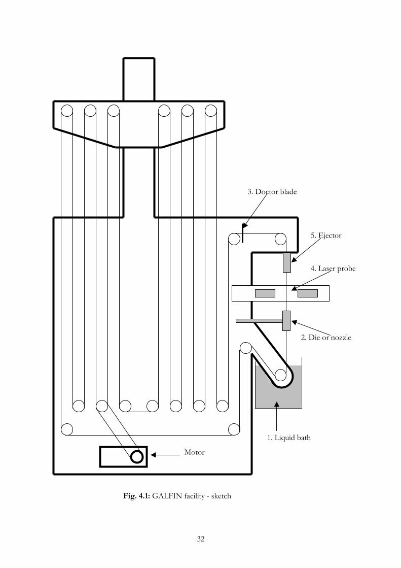
4.1 Introduction In the previous chapters, the theory of wire coating and wire coating instabilities has been described. Since the goal of the project is to investigate experimentally the behaviour of the instabilities, in this chapter a brief description of the experimental set-up, the measurement chain and the data processing will be given. 4.2 GALFIN facility GALFIN stays for GALvanisation des FILs (wire galvanisation process). A sketch of the set-up is shown in figure (4.1), while the picture is reported in figure (4.2). The main parts are: the liquid bath (1), where the wire pass trough in order to be covered by the liquid; the nozzle or the die (2), where the thickness of the coating is controlled, the probes (4), in order to measure the coating thickness. A doctor blade (3) is required to clean the wire after the measure. The liquid used is silicon oil having different values of viscosity, density and surface tension. A complete description of the facility can be found in [1] [3]. The position of the probe (4) can change in vertical direction, so that it’s possible to perform measurements at different distances from the liquid bath or from die or nozzle. During the experiments it was necessary to introduce an ejector (5) because the wire covered by the liquid, touching the first pulley after the bath, produces a run-back flow that interferes with the coating. A tube (6) connects the ejector to a filter in order to recover the oil.
31
3. Doctor blade
5. Ejector
4. Laser probe
2. Die or nozzle
Motor
1. Liquid bath
Fig. 4.1: GALFIN facility - sketch
32

3. Doctor blade
6. Tube to the filter
5. Ejector
4. Laser probes
2. Die or nozzle
1. Liquid bath
Fig. 4.2: GALFIN facility - picture
In figure (4.2) a picture of the GALFIN facility is shown and all the interesting parts described in the sketch previously shown are visible. In the following table, the typical values of the wire velocity and the fluid properties used reported.
V 0.1÷3 m/s Wire velocity ρ 900÷970 Kg/m3 Liquid density µ 0.01÷0.5 Pa·s Liquid viscosity σ 0.015÷0.025 N/m Liquid surface tension d 0.1÷3·10-3 m Wire diameter
33
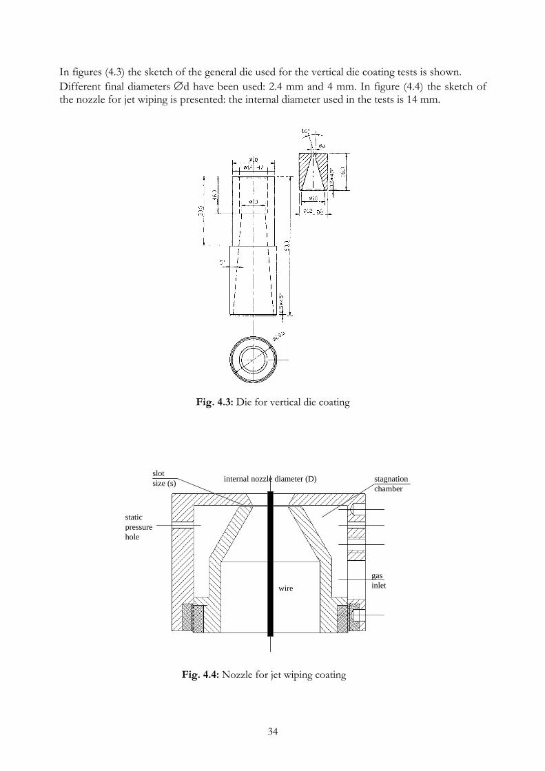
In figures (4.3) the sketch of the general die used for the vertical die coating tests is shown. Different final diameters ∅d have been used: 2.4 mm and 4 mm. In figure (4.4) the sketch of the nozzle for jet wiping is presented: the internal diameter used in the tests is 14 mm.
Fig. 4.3: Die for vertical die coating
internal nozzle diameter (D)
staticpressurehole
wire
stagnation chamber
gasinlet
slotsize (s)
Fig. 4.4: Nozzle for jet wiping coating
34

4.3 Measurement chain In the experimental investigations, different kinds of techniques have been used in order to choose the more appropriate to follow the wave shape and to detect the instability. The main purpose is to have the possibility to measure the wave amplitude and wavelength with a good accuracy. Since also the wave speed is an important parameter, a complete new technique has been used in order to be able to measure both long and short ones. In the following paragraph, all the techniques used will be described. In all the cases considered, the following steps are present in the measurement chain: • The probe, which is sensitive to the physical quantity we want to measure (the thickness as
function of time) • The transducer, which transforms the variation of a physical characteristic of the probe in a
more treatable signal (voltage) • A data processing in order to obtain from the previous signal the information concerning
the mean coating thickness, the wave amplitude and the wavelength. 4.3.1 CCD camera The technique used up to this project has been the CCD camera. For more details on the use of it and on the digital image processing, good references are [1] [2] [3] [4]. After different attempts during the preliminary tests in the frame of this project, this technique was abandoned because of several reasons: • To have a good mean value of the wave amplitude and of the wavelength, a great amount of
pictures is needed (at least 100) • The maximum frequency that can be reached is 25 Hz, too low to follow small wavelength • The measurement of the wave amplitude and wavelength was performed “by hand” for
each image measuring the number of pixel (the length in millimetre is obtained via calibration image)
• The calibration is needed each time the camera is moved, since the distance between the wire and the CCD sensor can change and the ratio pixel/mm changes
• For the calibration, it is assumed that the wire diameter is the nominal one. On the contrary, measuring the wire diameter it was found that there is a big dispersion around the nominal value. When the calibration is performed, it is possible that the part of the wire investigated does not correspond to a value close to the nominal one, so that the calibration itself becomes meaningless. To avoid this problem, a probe like the hot wire support (without the wire) was built in the present work and used in order to guarantee a fixed distance as reference.
35

Known distance
SupportWire
Fig. 4.5: Calibration for the CCD camera • If the camera is not exactly perpendicular to the wire, it is possible to observe a divergence
of the image due to an optical effect (a “pillow” effect as for the computer monitor) which is not desired if the wave amplitude has to be measured.
Deformed shape
Real shape
Investigation window
Fig. 4.6: Optical deformation • The typical value of the wavelength observed in the simple withdrawal and die coating is of
the order of 20 mm. Since to have a good compromise for the resolution (10 µm) a window of about 6 mm by 6 mm is needed, it is impossible to observe a complete wave in only one image. That is the main reason for abandoning this technique.
In figure (4.7) the measurement chain for the CCD camera technique is sketched. The signal from the camera is recorded using a common video recorder: the single images are obtained by appropriate software and then they are processed using digital image processing.
Fig. 4.7: CCD camera technique
recorder
CCD camera6 mm
6 mm fsampling=25 Hz
resol. =10 µm
36

4.3.2 Laser beam probe A new probe was available at VKI at the beginning of the project. Its fundamental principle is based on laser beams scanning an area as shown in figure (4.8). Between the laser source and the receiver there is the wire and knowing the scanning frequency and time for which the light is interrupted (by the wire) allows the measurement of the diameter of the wire covered by the coating. The scanning frequency is very high: 200 Hz for each beam, but for technical reasons is not possible to access the data at that frequency. The data are acquired at a frequency of about 3 Hz which too low for the aim of this project, since small waves can not be followed. For this reason this technique is used to measure only the mean coating thickness. In figure (4.8) a sketch of the probe is presented and in figure (4.9) the laser beam measurement chain.
Laser beamsLaser source
Photo sensor Wire
Fig. 4.8: Laser beam probe Rotating laser beam
fsampling =3 Hz resol. =0.1 µm
Fig. 4.9: Laser beam technique The probe is provided with relative software, so that a file can be saved containing directly the values of the diameter in mm.
37

The advantages of this technique are: • no calibration is required (the instrument has a pre-calibrated piece inside as a reference) • the wire can oscillate (without going out of the investigated volume) without producing
undesired effects • it is possible to check the ovalization of the wire since the probe measures the diameter in
two perpendicular directions • very high spatial resolution: order of 0.1 µm. 4.3.2 Laser sheet probe The previous techniques are not powerful enough for the purpose of this study, since the CCD camera has all the limitations exposed and the laser beam probe can be used only for the mean thickness since even if the resolution is very high, the sampling frequency is too low. A new probe has been introduced to satisfy the requirements of both good spatial resolution and high sampling frequency in order to follow the waves on the surface of the coating in a wide range of wavelength. In the following figure (4.10) the sketch of the measurement technique is shown.
Receiver
Laser source
5 mm
Laser sheet
fsampling =3 kHz resol. =5 µm
Fig. 4.10: Laser sheet technique The basic principle is similar to the laser beam probe: a laser sheet 1 mm thick and 5 mm wide is produced by the laser source. A receiver is set in front of the laser source and the wire is positioned between the source and the receiver. The light received by the receiver is linearly proportional (with a negative slope of the curve) to the diameter of the wire: if the diameter increases, the signal from the receiver decreases. For this technique a calibration is needed: it has been performed using reference wires of well-known diameter. Knowing the voltage at the output of the instrument and the corresponding diameter, a linear regression has been used in order to obtain the calibration curve.
38

This probe is a very good instrument when dealing with instabilities because the sampling frequency can reach 3 kHz with a good spatial resolution (order of 5 µm). If the wire moves within the laser sheet there are no problems since the light received is always the same; but if during the movement the wire goes out of the volume probe, than the measurement is completely wrong. A great attention must be paid to this problem, checking before acquiring data if the wire is in the right position. Another problem found is that the optical lens used in the laser source and receiver can get dirty because of the hard environment: oil droplets are dangerous for the probe because they cause optical deformations and a reduction of the output signal due to not transparent medium. To avoid this, a device to cover and guarantee a better protection has been added on the top of the probe. One important remark is that this probe has been introduced for the first time in the present study of wire coating instabilities. It represents a great improvement to the previous techniques since it could have been impossible to retrieve all the information needed using the CCD camera or the laser beam sensor. Another important remark is that with this instrument it has been possible to measure the wave speed. This goal has been reached by using two probes set at a certain known distance and comparing the two signals obtained (see figure (4.11)). Fig. 4.11: Laser sheet technique – wave speed measurement
39

4.4 Data processing The data processing procedure is schematically presented in figure (4.12):
t∆
h
t
ci cr
correlationCross
A h
xFFT-1
FFT
h0Ak
λ
λk
λ
h
t
CCD + DIP Laser sheet Laser beam
Fig. 4.12: Data processing procedure Using one of the three previous techniques, it is always possible to obtain a signal that is function of the time, because the sampling frequency is known. In the wave velocity can be measured, the signal can be transformed as a function of space. If the wave velocity can not be measured, its value can be computed by the theory, so that the same transformation between time and space can be performed. The only parameter affected by the velocity chosen for the transformation is the wavelength, linearly proportional to it. The signal obtained is processed in order to retrieve the most important parameters: the mean thickness, the wavelength, the wave amplitude, the wave velocity and the amplification factor. For this purpose, a program in Mathcad has been developed in the frame of this project, in order to process automatically the data obtained by the measurements. In the following paragraph a brief description of the characteristic steps of the program is given, while the complete Mathcad worksheet is found in appendix. 4.4.1 General philosophy of the program The way in which the program operates can be schematically summarised:
1. Transformation of the signal obtained from the probe into the diameter (wire + coating thickness) using the calibration curve
40

2. Computation of h(x), subtracting the mean wire diameter to the signal obtained in (1.) 3. Computation of the mean thickness value h0, averaging the signal obtained at point (2.) 4. Fast Fourier Transform on the signal at point (2.) 5. Computation of the wave velocity cr from the experiments, if it is possible, or from the
theory 6. Transformation of the spectrum obtained at point (4.) to the spectrum function of the
wavelength (λ=V/f ), using the wave velocity computed at point (5.) 7. Detection of the wavelength λ of interest, looking at the spectrum at point (6.) 8. Reconstruction of the signal containing only the wavelengths detected at point (7.) 9. Evaluation of the wave amplitude A of the signal obtained at point (8.) 10. Evaluation of the amplification factor ci
The first remark is that with this program it is possible to have an automatic procedure to compute the most important parameter involved in the stability study. The only point that for the moment is not yet automated is (7.) since it requires a certain “human contribution” in order to decide the wavelength corresponding to the peaks observed. The main problem, actually, is that in the power spectrum has a not always sharp peak because the data come from experiments. In the following paragraphs, a brief description of the most important parts of the program will be given. 4.4.2 Mean final thickness measurement This part is the easiest since only an average has to be performed. The original data are first transformed in [mm] using the calibration curve obtained during the calibration procedure of the instrument before experiments. After this, the mean wire diameter has to be subtracted in order to obtain the coating thickness. Since the wire diameter is not constant and the mean diameter can be different from the nominal value, before performing each set of tests, the diameter of the wire without coating is measured to obtain the mean wire diameter to subtract. Once the coating thickness has been extracted, by a simple averaging the mean coating thickness is obtained. 4.4.3 Wave velocity measurement The wave velocity is an important parameter that influences the measurement of the wavelength and for this reasons it must be measured accurately. The only possibility to measure it directly is recording the wave shape at two different stations and comparing them. The best way to do it is to perform a cross-correlation between the two signals, finding the time delay needed to go from the first probe to the second one. Knowing the distance
t∆s∆ between the two measurement
points, the wave velocity is easily obtained:
tscr ∆
∆= (4.1)
41

This procedure is possible only if two identical probes are available. One problem is that to obtain the cross-correlation it is necessary to have the two signals with the same mean value. This is due to the fact the cross-correlation procedure corresponds to shifting one signal with respect to the other, until a good agreement is obtained and this is correctly performed is only if the two signals fluctuate around the same mean value. An example of the way in which the wave velocity is obtained is found comparing the following figures. In figure (4.13) the two signals recorded at two different stations are shown. The shape is clearly the same, but they are shifted by a certain constant due to the fact that a certain time is required to go from the station closer to the liquid bath to the one far from it. Shifting one of the signals with respect to the other one, using the time delay t∆ provided by cross-correlation, very good agreement is obtained as shown in figure (4.14).
C
14 14.5 15 15.5 16 16.5 17 17.5 180.65
0.7
0.75
0.8
0.85
t [s]
diam
eter
[mm
]
Fig. 4.13: Two signals measured at two different points
C
14 14.5 15 15.5 16 16.5 17 17.5 180.65
0.7
0.75
0.8
0.85
t [s]
diam
eter
[mm
]
Fig. 4.14: Two signals measured at two different points after shifting
42

In figure (4.15) the sketch with the two probes is shown. D is the distance between the two probes, while L is the distance of the lower probe from the liquid bath, in the case of simple withdrawal tests, from the die, in the case of die coating and from the nozzle in the case of jet wiping coating. The minimum value of D is 40 mm, due to the supports; while the minimum value of L depends on the kind of test. The idea is to change D and L in order to check if the wave velocity is always the same.
Fig. 4.15: Position of the two probes
L
D
V 4.4.4 Wavelength detection The wavelength is simply given by the velocity divided by the frequency. The FFT is performed on the signal function of time and then the spectrum is transformed from function of frequency to function of space in order to measure the wavelength. Usually, in one signal, there is more than a single peak, corresponding to more than one wavelength, which means than different waves are observed. The main problem in the detection of the wavelength is that the peaks are not always sharp and it is difficult to decide which range of wavelength are involved and have to be considered for that peak: that is the reason why this procedure can not be completely automatic. An example of this kind of problem is shown in figure (4.16) Referring to figure (4.16), from 20 mm to about 35 mm the wavelengths can be considered belonging to the first peak at λ=26.7 mm, while from λ=35 mm to λ=45 [mm] the wavelengths can be considered belonging to the second peak at λ=40.2 mm. The same can be applied for the third peak at λ=80.4 mm.
43

0 20 40 60 80 1000
0.5
1Wave length
Wavelength [mm]
Pow
er sp
ectru
m
ciao
Fig. 4.16: Typical power spectrum
Since more than one wavelength is detected, the relative importance of each of them can be taken into account computing the ratio between the integral of the spectrum around the peak and the integral of the entire spectrum. 4.4.5 Wave amplitude measurement For each of the previous observed wavelengths, it is possible to compute the corresponding amplitude. To do this, it is necessary to reconstruct the signal having only the wavelength in the range of interest, decided during the previous step. The power spectrum is multiplied by a function that is equal to 1 in the range we want to keep the wavelength and equal to zero elsewhere, as shown in figure (4.17).
λ λ
Fig. 4.17: Filtering procedure Once the spectrum limited only to a certain wavelength has been obtained, the inverse FFT is applied in order to retrieve a signal function of space having only a certain range of wavelength,
44
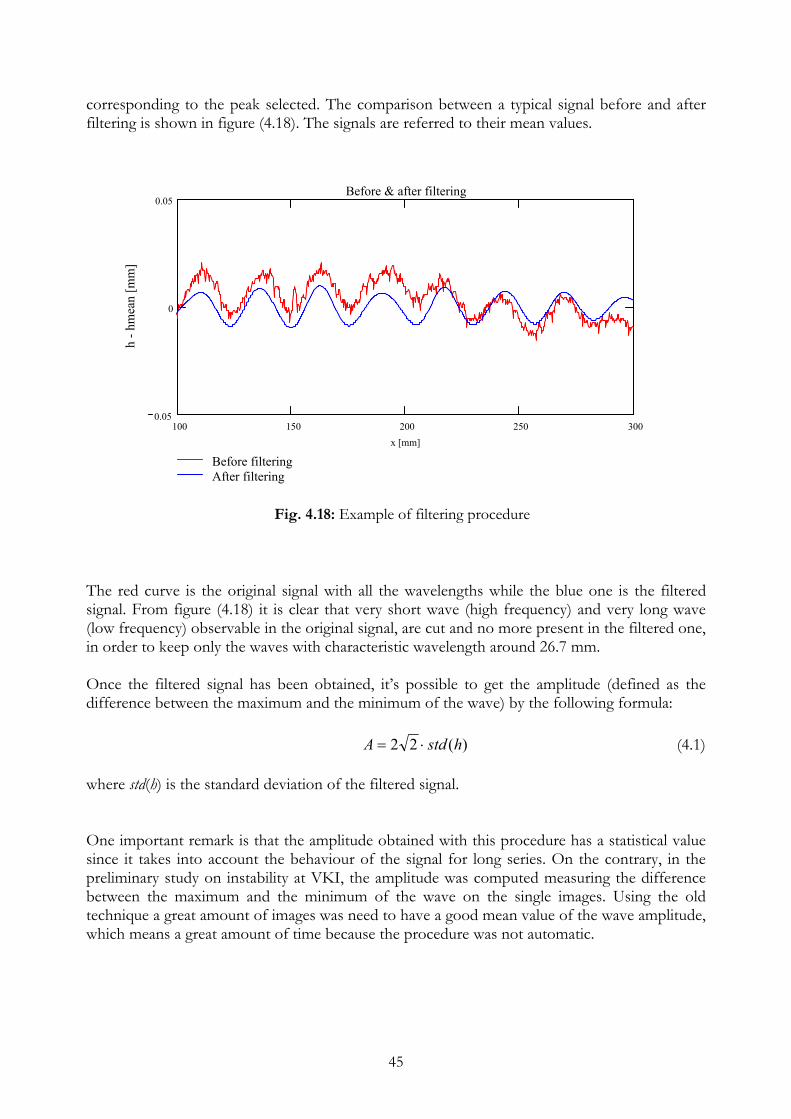
corresponding to the peak selected. The comparison between a typical signal before and after filtering is shown in figure (4.18). The signals are referred to their mean values.
100 150 200 250 3000.05
0
0.05
Before filteringAfter filtering
Before & after filtering
x [mm]
h - h
mea
n [m
m]
ciao
Fig. 4.18: Example of filtering procedure
The red curve is the original signal with all the wavelengths while the blue one is the filtered signal. From figure (4.18) it is clear that very short wave (high frequency) and very long wave (low frequency) observable in the original signal, are cut and no more present in the filtered one, in order to keep only the waves with characteristic wavelength around 26.7 mm. Once the filtered signal has been obtained, it’s possible to get the amplitude (defined as the difference between the maximum and the minimum of the wave) by the following formula:
)(22 hstdA ⋅= (4.1) where std(h) is the standard deviation of the filtered signal. One important remark is that the amplitude obtained with this procedure has a statistical value since it takes into account the behaviour of the signal for long series. On the contrary, in the preliminary study on instability at VKI, the amplitude was computed measuring the difference between the maximum and the minimum of the wave on the single images. Using the old technique a great amount of images was need to have a good mean value of the wave amplitude, which means a great amount of time because the procedure was not automatic.
45

4.4.6 Amplification factor measurement The measurement of the wave amplitude itself is interesting in the coating process, since if it non-uniformity of the surface is smaller than a threshold value, the coating can be considered of good quality. More information can be obtained measuring the amplitude at different distances, since it gives an idea about the stable or unstable behaviour of the liquid film. If the wave amplitude increases with the space (or time) instability is observed, if it decreases the flow is stable: this is the reason why the measurement of the amplitude at two different stations is an essential requirement for understanding the stability behaviour of the coating. One parameter that can be evaluated in order to check the amplification or damping is the amplification factor. Experimentally, it can be obtained from the following considerations. The wave shape at the free surface can be modelled as:
( )
∆−=−=
waveVxcxiActxiAA exp)(exp 00 (4.2)
where c is the complex velocity in which the imaginary part is ci, the amplification factor. Measuring the amplitude at two different stations, the experimental amplification factor is given by the expression:
∆
=2
1lnAA
sV Expwave
ic (4.3)
where V is the wave velocity measured in the experiments, Expwave s∆ is the distance between the two probes used to measure the wave velocity and and the wave amplitudes measured respectively at higher level and lower level.
1A 2A
46

Chapter 5
Uncertainty evaluation 5.1 Introduction Before starting the measurements, it is necessary to compute the uncertainty associated to the value that will be obtained from the measure itself. The physical quantities that are measured in the experiments are: • The mean final thickness • The wave velocity • The wavelength • The wave amplitude In order to compare these measured quantities with the ones predicted by the theory it is necessary to know the following parameters: • The wire velocity • The viscosity of the oil • The density of the oil In the following paragraphs, the uncertainty for each case will be considered.
47

5.2 Probe calibration The first uncertainty is in the coefficients derived for the calibration curve of the laser sheet probe. The relation is:
bVad += (5.1) where d is the diameter (wire +coating) measured, a is the shift, b the slope of the regression line and V the output voltage of the probe. The uncertainty at this step is in the coefficients a and b. It is possible to estimate it, since the uncertainty on the diameter imposed for the calibration is known and also the uncertainty of the voltmeter used to read the value in volts. From the estimation of uncertainty it is found:
002.0=aδ mm
003.0=bδ mm/Volt These two uncertainties are referred to the diameter measured in mm and the voltage in volts. They are used for the estimation of the uncertainty in the diameter measured. 5.3 Diameter measured The final diameter measured is given by (5.1), which means that the uncertainty can be computed by:
( ) ( ) ( )222 VbbVad δδδδ ++= (5.2) Since δV is known and given by 0.001 and the other uncertainties have been previously computed, δd is found of the order:
δd=0.008 mm This uncertainty is referred to the diameter in mm and since the expected typical values for d is around 3 mm, the error is 0.26%. 5.4 Wave velocity The wave velocity is given by the formula:
tsVwave ∆
∆= (5.3)
48

where is the distance measured between the probes and s∆ t∆ the time computed by cross correlation. The uncertainty in the wave velocity is:
2
2
2
∆
∆∆−
+
∆∆
= tts
tsVwave δδδ (5.4)
s∆δ maximum is 1 mm =0.001 m, while t∆δ is related to the cross-correlation and sampling
frequency and its maximum is of the order of 0.001 s (the inverse of the sampling frequency). Substituting these values in (5.4), the uncertainty in the wave velocity is found:
δVwave=0.003 m/s Since the expected absolute wave velocity is about 0.5 m/s, the error is smaller than 1%. 5.5 Wavelength The wavelength is proportional to the wave velocity, and given by the formula:
fVwave=λ (5.5)
where f is the frequency at which the peak is detected in the power spectrum. Supposing that the uncertainty in the frequency is negligible,
fVwaveδ
δλ = (5.6)
so that the uncertainty for the wavelength is of the order of
δλ=0.0005 m 5.6 Wave amplitude The uncertainty for the wave amplitude is of the same order of the one for the diameter measured, which means order of 8 µm.
49

5.7 Wire velocity The uncertainty for the wire velocity is due to the calibration curve of the GALFIN facility and to the value, in Hz, read on the display of the facility. Using the same technique applied for the laser probe, since the calibration curve is linear, the uncertainty is found to be of the order
δV=0.01 m/s Another possible source of error in the wire velocity is the fact that ideal no-slip condition between the whirl driven by the motor and the wire could not be completely true because of the presence of residual oil on the wire. 5.8 Viscosity of the oil Since the theoretical model developed at VKI is very sensitive to value of the viscosity, the last must be measured. The uncertainty found measuring the dependence of the viscosity on the temperature is due to the uncertainty on the temperature, which is 0.1°C and the uncertainty of the digital display of the instrument which is used. Considering the uncertainty in the regression curve and the one for the ambient temperature, the final uncertainty for the viscosity is
δµ=0.001 Pa·s which correspond to a relative error smaller than 1% 5.9 Density of the oil Also the density of the oil has been measured in order to check and compare it with the value given. The mass and the volume have been measured and then the following relation applied:
Volm
=ρ (5.7)
so that the uncertainty in the density is :
2
2
2
−+
= Vol
Volm
Volm δδδρ (5.8)
substituting δm=0.001 g and δVol=0.1 ml, for m=10 g and Vol=10 ml, δρ=0.01 g/ml, which means:
δρ=1 kg/m3
50
Chapter 6
Simple withdrawal results 6.1 Introduction In this chapter the main results obtained by the experiments performed on GALFIN facility concerning the simple withdrawal case will be presented. The laser beam probe has been used just to check if the thickness measured by the laser sheet probe and the laser beam one was the same (within experimental accuracy). Once the agreement between the results obtained with these two different techniques has been proved the results extracted using the laser sheet probe will be presented. The description of the experimental results will be correlated to the theory, discussing the agreement and disagreement and explaining the reasons. In all the tests, the wire velocity was lower than 0.4 m/s. Tests at higher velocity and using the same oil were impossible because the diameter measured (wire diameter + coating thickness) exceeded 5 mm, which is the maximum that can be measured by the laser sheet probe. Lower velocity was not useful, especially because wire coating is an industrial process and high wire velocity is required. The typical value of the fluid properties and test conditions are reported in the following table:
ρ 951 [kg/m3] Density µ 0.114 [Pa·s] Viscosity σ 0.02 [Pa/m] Surface tension r0 1·10-3 [m] Wire radius V 0.12÷0.4 [m/s] Wire velocity
51
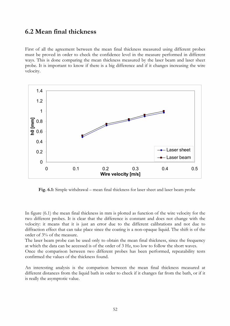
6.2 Mean final thickness First of all the agreement between the mean final thickness measured using different probes must be proved in order to check the confidence level in the measure performed in different ways. This is done comparing the mean thickness measured by the laser beam and laser sheet probe. It is important to know if there is a big difference and if it changes increasing the wire velocity.
0
0.2
0.4
0.6
0.8
1
1.2
1.4
0 0.1 0.2 0.3 0.4 0.5Wire velocity [m/s]
h0 [m
m]
Laser sheetLaser beam
Fig. 6.1: Simple withdrawal – mean final thickness for laser sheet and laser beam probe In figure (6.1) the mean final thickness in mm is plotted as function of the wire velocity for the two different probes. It is clear that the difference is constant and does not change with the velocity: it means that it is just an error due to the different calibrations and not due to diffraction effect that can take place since the coating is a non-opaque liquid. The shift is of the order of 3% of the measure. The laser beam probe can be used only to obtain the mean final thickness, since the frequency at which the data can be accessed is of the order of 3 Hz, too low to follow the short waves. Once the comparison between two different probes has been performed, repeatability tests confirmed the values of the thickness found. An interesting analysis is the comparison between the mean final thickness measured at different distances from the liquid bath in order to check if it changes far from the bath, or if it is really the asymptotic value.
52

0
0.2
0.4
0.6
0.8
1
1.2
0 0.1 0.2 0.3 0.4 0.5Wire velocity [m/s]
h0 [m
m]
L=350L=280L=180
Fig. 6.2: Simple withdrawal – mean final thickness for different distances from the bath
From figure (6.2) it is evident that the mean thickness value measured for different distances from the bath does not change. This means that the final thickness is really an asymptotic value and that the measure is repeatable. In the two previous figures, dimensional parameters have been used in order give an idea of the characteristic values observed for the simple withdrawal. In the following figures, dimensionless parameters will be used, and the experimental results will be compared with the theoretical ones.
0
0.2
0.4
0.6
0.8
1
1 1.2 1.4 1.6 1.8 2 2.2 2.4Ca
h0/r0 L=180 mm
L=350 mm
VKI Theory T=20º C
VKI Theory T=15º C
Fig. 6.3: Simple withdrawal – mean final thickness compared with theory 53

In figure (6.3) the mean final thickness is shown. Two different distances from the liquid bath are considered: 180 mm and 350 mm and the tests have been performed for 10 different velocities. The experimental results are compared with the theory developed at VKI in the previous years [3]. The results are plotted in dimensionless parameters: Capillary number (µV/σ ), which represents the dimensionless wire velocity, versus h0/r0 , the mean final thickness divided by the radius of the wire. Since the radius r0 is equal to 1 mm, from the figure the thickness in mm is available. The main conclusion that can be drawn from figure (6.3) is that when the velocity is increased, the mean final thickness increases and the experimental results are in very good agreement with the VKI theory. Two curves from the VKI model are plotted in figure (6.3) because the ambient temperature was not exactly known: the model is very sensitive to the value of the viscosity and the viscosity is itself very sensitive to the temperature. Since the temperature was between 15° C and 20° C the two curves corresponding to these values are shown, in order to evaluate the error in the two cases. The worst case is for T=20° C, since in this case the viscosity is lower and the mean final thickness is smaller: the error is of the order of 6-7%, which is within experimental accuracy. In the most realistic case of ambient temperature equal to 15° C, the agreement is better and the error is of the order of 3-4%. Finally, comparing the mean final thickness at different distances from the bath (180 and 350 mm), we can say that the thickness is really the “final” one, since the distance does not affect it. 6.3 Wave velocity In figure (6.6) experimental results for five different test configurations are compared with the theory by Lin & Liu [8].
0
0.05
0.1
0.15
0.2
0.25
0.3
0.35
0 0.1 0.2 0.3 0.4 0.5V [m/s]
Wav
e ve
loci
ty [m
/s]
Experiments L=38, D=4 Experiments L=31, D=11Experiments L=31, D=19 Experiments L=45, D=4Experiments L=29, D=4 Lin & Liu Theory [8]
Fig. 6.6: Simple withdrawal – wave velocity experimental and theoretical values
54

The wave velocity is plotted versus the wire velocity. The axes start from zero in order to see the slope, since it represents the ratio between the wave velocity and the wire velocity. The different tests have been performed changing the distance from the liquid bath (L) from 29 cm to 45 cm. It was impossible to test lower or higher distances simply because otherwise big modifications to GALFIN facility were needed. The distance between the two probes is between 4 cm and 19 cm: the limitations are again due to the geometry of the facility. From figure (6.6) it is clear that in all the experiments the value of the wave velocity increases increasing the wire velocity, following the behaviour of a straight line. For wire velocities smaller than 0.35 m/s this is really true, while for higher values there is a deviation from the ideal line and the observed values are smaller. This is probably due to non-linear phenomena that happen at higher velocity or to the fact that the wire velocity is not exactly the one supposed because of a slight slip on the whirls. Comparing the experimental results with the theoretical values predicted by Lin & Liu theory presented in chapter 3, a good agreement is found and the maximum error is observed at high velocity. The explanation of this difference is probably that the theory is linear and if non-linear phenomena occur in that range of velocities, they cannot be taken into account. Anyway, the difference is within 10% that can be considered a not bad result. The most important remark is that in all the tests, the experimental wave velocity, for a fixed wire velocity, is always the same independently on the distance from the bath or between the two probes. This is a very important conclusion because of different reasons. First of all the experiments can be considered repeatable since always the same value is found (within experimental uncertainty). Second, changing the distance from the liquid bath, the wave velocity does not change, which means that it is a constant value as predicted by the theory, and it is not function of L. Finally, changing the distance between the probes, always the same value is found, meaning that it should be the correct one, since it has been obtained in different ways, changing the time shift and D. In figure (6.7) the wire velocity has been made dimensionless introducing the Capillary number, while the wave velocity is multiplied by (µ/σ), following the same idea. Using dimensionless form is useful for further comparison.
0
0.4
0.8
1.2
1.6
2
0 0.4 0.8 1.2 1.6 2 2.4Ca
Wav
e ve
loci
ty *
µ/ σ
Experiments L=38, D=4 Experiments L=31, D=11
Experiments L=31, D=19 Experiments L=45, D=4
Experiments L=29, D=4 Lin & Liu Theory [8]
Fig. 6.7: Simple withdrawal – wave velocity experimental and theoretical in dimensionless form
55

6.4 Wavelength Once the experimental wave velocity has been measured, it can be used in order to pass from the signal as function of time to the signal as function of space. Since the wavelength is extracted by the power spectrum, an example of the typical result obtained by the developed program is shown in figure (6.8).
sim 20000 30000.. s_coat sim 0
0 5 10 15 20 25 30 35 40 45 50 55 60 65 700
0.2
0.4
0.6
0.8
1
Wavelength [mm]
Pow
er sp
ectru
m
Fig. 6.8: Simple withdrawal – typical power spectrum From figure (6.8) the typical values of the wavelength detected in the simple withdrawal can be obtained. There is one main peak at about 20 mm and another one, very strong, at bout 57 mm. Another characteristic peak is found at about 28 mm, but its energy content is smaller than in the other cases.
56
c
100 120 140 160 180 200 220 240 260 280 300 320 340 360 380 4000.6
0.65
0.7
0.75
0.8
x [mm]
diam
eter
[mm
]
The measured wavelengths can be seen also in the signal function of space, reported in figure (6.9).
Fig. 6.9: Simple withdrawal – typical signal function of space (referred to figure (6.8))
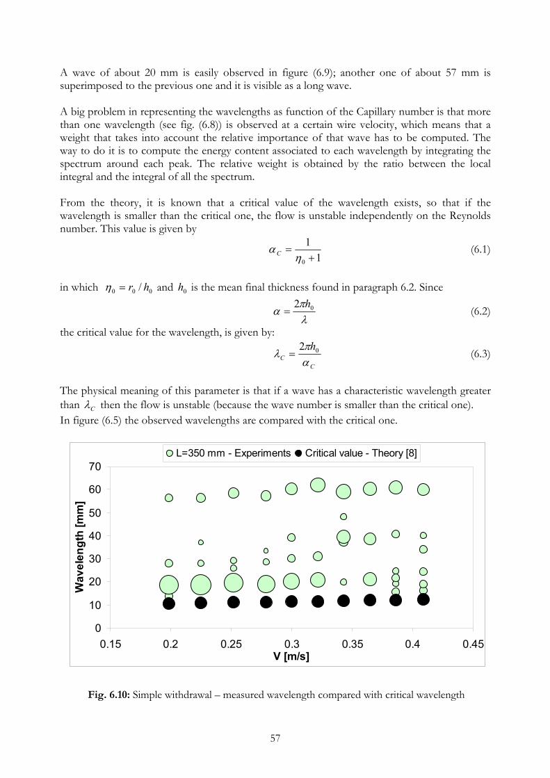
A wave of about 20 mm is easily observed in figure (6.9); another one of about 57 mm is superimposed to the previous one and it is visible as a long wave. A big problem in representing the wavelengths as function of the Capillary number is that more than one wavelength (see fig. (6.8)) is observed at a certain wire velocity, which means that a weight that takes into account the relative importance of that wave has to be computed. The way to do it is to compute the energy content associated to each wavelength by integrating the spectrum around each peak. The relative weight is obtained by the ratio between the local integral and the integral of all the spectrum. From the theory, it is known that a critical value of the wavelength exists, so that if the wavelength is smaller than the critical one, the flow is unstable independently on the Reynolds number. This value is given by
11
0 +=
ηαC (6.1)
in which 000 / hr=η and is the mean final thickness found in paragraph 6.2. Since 0h
λπ
α 02 h= (6.2)
the critical value for the wavelength, is given by:
CC
hαπ
λ 02= (6.3)
The physical meaning of this parameter is that if a wave has a characteristic wavelength greater than Cλ then the flow is unstable (because the wave number is smaller than the critical one). In figure (6.5) the observed wavelengths are compared with the critical one.
0
10
20
30
40
50
60
70
0.15 0.2 0.25 0.3 0.35 0.4 0.45V [m/s]
Wav
elen
gth
[mm
]
L=350 mm - Experiments Critical value - Theory [8]
Fig. 6.10: Simple withdrawal – measured wavelength compared with critical wavelength
57

Dimensional parameters have been used in figure (6.10) in order to give an idea of the physical values observed. The black bubbles represent the critical value of the wavelength that is of the order of 11 mm and increases with the velocity, because the mean final thickness increases with the velocity producing smaller 0η so that by formula (6.1) Cα increases. The observed wavelengths are in a range between 15 mm and 60 mm. They have been computed considering the real wave velocity measured by experiments. The relative importance of each wavelength observed at a certain velocity is proportional to the size of the bubble in figure (6.10). A particular behaviour, never observed before, is that for low wire velocity (from 0.2 m/s to 0.3 m/s) the instability is dominated by short waves, with typical value of 20 mm for the wavelength. For velocities grater than 0.3 m/s the long waves have more importance, even if peaks at short wavelengths are still observed. This means that the energy content goes from short to long waves as the velocity is increased. The physical reason of this behaviour can be found considering that short waves are usually stable while long ones becomes unstable. At low velocity the short waves are observed because the long ones have not jet developed, while increasing the velocity the long wave instability dominates, moving the energy content of the spectrum to higher wavelengths.
0
5
10
15
20
25
30
35
1 1.2 1.4 1.6 1.8 2 2.2 2.4Ca
Wav
elen
gth/
lc
L=350 mm - Experiments Critical value - Theory [8] Fig. 6.11: Simple withdrawal – measured wavelength compared with critical wavelength In figure (6.11) dimensionless parameters are used: instead of the wire velocity, the Capillary number is considered and instead of the absolute wavelength, the wavelength dived by the capillary length. The last is a characteristic length that depends on the fluid properties:
glC ρσ /2= .
58

The previous figure was referred to the wavelength measured far from the liquid bath at a distance L=350 mm. In order to check the dependence of the observed wavelength on the distance from the bath, other measures have been carried out at smaller distance L=180 mm.
0
5
10
15
20
25
30
35
1 1.2 1.4 1.6 1.8 2 2.2 2.4Ca
Wav
elen
gth/
lc
L=180 mm - Experiments Critical value -Theory [8] Fig. 6.12: Simple withdrawal – measured wavelength compared with critical wavelength The main wavelengths observed at L=180 mm are the same as L=350 mm, as shown in figure (6.12). All of them are above the critical value as predicted by the theory. In figure (6.12) the wavelengths shift from short to long waves is clearer: big bubbles characterise the dimensionless wavelengths around 10-12 only for low Capillary number up to 1.6. For grater values of Ca, the biggest bubbles are distributed around a value of about 35. 6.4 Wave amplitude The amplitudes measured at 180 mm and 350 mm from the liquid bath have been reported in figure (6.13). The curves show that the amplitude decreases when the velocity of the wire is increased. This information is important, because if the uniformity of the coating is a constrain, small amplitude is considered a positive characteristic. If the amplitudes at different distances from the bath are compared, the main conclusion is that the flow is unstable at low velocity, going to stable behaviour at high velocity. This conclusion comes from the observation that the amplitude at higher level is greater than the amplitude at lower level, meaning that the wave is amplified (figure (6.13)).
59

0
0.01
0.02
0.03
0.04
0.05
1 1.2 1.4 1.6 1.8 2 2.2 2.4Ca
A/h
0
L=350 mmL=180 mm
Fig. 6.13: Simple withdrawal – wave amplitude at two different distances from the bath A better way to understand the stability or instability of the flow measured experimentally is to plot the experimental amplification factor compared with the theoretical one.
-0.2
0
0.2
0.4
0.6
0.8
1 1.2 1.4 1.6 1.8 2 2.2 2.4Ca
Ci
ExperimentsTheory - Lin & Liu [8]
Fig. 6.14: Simple withdrawal – theoretical and experimental amplification factor
60

61
As shown in figure (6.14), both the experimental and theoretical amplification factors are positive, fact that confirms the behaviour seen in figure (6.13). Increasing the Capillary number, they decrease, meaning that the flow goes towards less instability. The agreement between theory and experiments is really surprisingly and within all the uncertainties due to the experimental technique. The only difference is observed at the highest velocity, where the experimental amplification factor is negative, while the theoretical one is positive. It is due the fact that high Capillary number the value of the amplitude is almost the same for both distances from the liquid bath and a very small error in one of them can produce a small positive or negative value of the experimental amplification factor. 6.6 Conclusions In this chapter, the results obtained from simple withdrawal experiments are presented and discussed. The repeatability of the thickness measurement using two different probes or the same one has been proved. For the mean final thickness, the VKI theoretical model has been validated by the experimental data, which are in good agreement with the predicted values. The wave velocity measured for different distances between the probes and for different distances from the liquid bath is compared with the theoretical value, finding that the measured wave velocity is always slightly lower than the predicted one. The maximum discrepancy, within 10%, is observed for high wire velocity. The wavelength analysis reveals the presence of more than a single wave for a fixed wire velocity. At low Capillary number the typical wavelength is 20-30 mm, while, when the wire velocity is increased, longer waves are observed with characterstic wavelength of 80-90 mm. Looking at the spectra, an energy transfer from low to high wavelength is observed, since the relative weight of the peaks changes increasing the wire velocity. Finally, the amplitude is considered: measuring it close to the liquid bath, a smaller value than the one measured further from the liquid bath is found. This means that amplification is observed and the flow is unstable. This is confirmed by the amplification factor computed from the experiments and compared with the one predicted by the theory. It is always positive, and for increasing velocity it decreases, going to zero, meaning that the instability is reduced when the wire velocity is increased.

Chapter 7
Die coating results 7.1 Introduction For the die coating, several tests have been performed in different configurations. In the case of vertical die coating, a small and big die have been used in order to check the dependence of the instability behaviour on the ratio between the final internal diameter and the diameter of the wire. Since dies with physical defects were available, they have been used to investigate the presence or absence of the instability when there is an evident cause of disturbance in the flow. In the following paragraphs, the vertical die coating tests will be first described, dividing results for the small and big die in two different section, and then the tests for dies with defects will be discussed. 7.2 Vertical die coating – small die Velocities higher than the ones for the simple withdrawal could be reached simply because in die coating the mean final thickness does not change changing the wire velocity. This means that there is not a limiting wire velocity for which the total diameter that has to be measured is greater than 5 mm, the maximum for the laser sheet probe. In the following table the fluid properties and geometrical characteristics are reported.
62

ρ 951 [kg/m3] Density µ 0.114 [Pa·s] Viscosity σ 0.02 [Pa/m] Surface tension r0 1·10-3 [m] Wire radius d 1.2·10-3 [m] Die radius V 0.12÷1 [m/s] Wire velocity
7.2.1 Mean final thickness Several tests have been performed at different distance L from the die, in order the check if there is any dependence of the mean final thickness on this parameter. In figure (7.1) the results are shown.
0
0.05
0.1
0.15
0.2
0 1 2 3 4 5 6Ca
h0/r0
L=10 mm L=45 mm
L=100 mm VKI Theory
Fig. 7.1: Die coating – mean final thickness at different stations The results obtained say that the mean final thickness measured at different distances from the die is almost the same, which means that it is actually the asymptotic value. Comparing the experimental results with the theory developed at VKI, we can see that there is a good agreement between them. All the experimental data are around the predicted value and the only apparently difference is due to the fact that from the theory the mean final thickness should not change changing the velocity, while from the experiments a slight dependence on the velocity is found. The explanation could be that the model is very simple and does not take
63
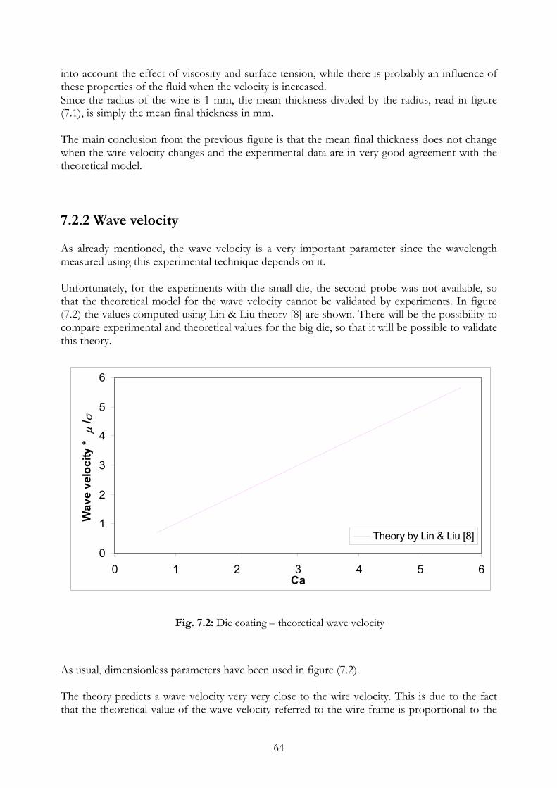
into account the effect of viscosity and surface tension, while there is probably an influence of these properties of the fluid when the velocity is increased. Since the radius of the wire is 1 mm, the mean thickness divided by the radius, read in figure (7.1), is simply the mean final thickness in mm. The main conclusion from the previous figure is that the mean final thickness does not change when the wire velocity changes and the experimental data are in very good agreement with the theoretical model. 7.2.2 Wave velocity As already mentioned, the wave velocity is a very important parameter since the wavelength measured using this experimental technique depends on it. Unfortunately, for the experiments with the small die, the second probe was not available, so that the theoretical model for the wave velocity cannot be validated by experiments. In figure (7.2) the values computed using Lin & Liu theory [8] are shown. There will be the possibility to compare experimental and theoretical values for the big die, so that it will be possible to validate this theory.
0
1
2
3
4
5
6
0 1 2 3 4 5 6Ca
Wav
e ve
loci
ty *
µ/ σ
Theory by Lin & Liu [8]
Fig. 7.2: Die coating – theoretical wave velocity As usual, dimensionless parameters have been used in figure (7.2). The theory predicts a wave velocity very very close to the wire velocity. This is due to the fact that the theoretical value of the wave velocity referred to the wire frame is proportional to the
64

velocity W0 (in the wire frame), which is the flow velocity computed at the air-coating interface. When the coating thickness is very small, W0 is also very small, which implies that the absolute wave velocity V-c0 is very close to V. This is clearly shown in figure (7.2), since the curve is a straight line with the slope very close to 1. 7.2.3 Wavelength The measure of the wavelength reveals a very strange behaviour of die coating. Waves are observed only at very low wire velocity, while at higher velocity they disappear. In figure (7.3) this situation is clearly summarised.
0
2
4
6
8
10
12
0 1 2 3 4 5 6Ca
Wav
elen
gth/
lc
Wavelength
No wave observed in this range
Fig. 7.3: Die coating – relative wave amplitude The wavelength has been made dimensionless dividing it by the Capillary length, which is close to 2 mm. Only one wavelength is observed for the first Capillary number, 0.7, and it is λ=20.2 mm (λ/lc=9.8). At higher velocity no waves are observed and the phenomenon seems to be quite strange. From the spectra, a very big difference is found between the first velocity (0.12 m/s) and the second one (0.28 m/s). The comparison between two characteristic spectra with and without wavelength is presented in figure (7.4) and (7.5)
65

c
0 5 10 15 20 25 30 35 40 45 50 55 60 65 70 75 80 85 90 95 1000
0.5
1
Wavelength [mm]
Pow
er sp
ectru
m
Fig. 7.4: Die coating – wavelength presence. V=0.122 m/s, Ca= 0.58, Go=0.483, T=0.76
c
0 5 10 15 20 25 30 35 40 45 50 55 60 65 70 75 80 85 90 95 1000
0.5
1
Wavelength [mm]
Pow
er sp
ectru
m
Fig. 7.5: Die coating – wavelength absence. V≥0.297 m/s, Ca≤1.35, Go=0.58, T≤0.27
The comparison between the two figures reveals a completely different behaviour of the wave when the velocity is increased. This is not so strange, because, as described in the theoretical part concerning the die coating, when the velocity is increased the amplification factor decreases. In the experiments, the Goucher number is always Go=0.483, since it depends on the characteristic of the fluid and on the wire radius, while the velocity increases between the first
case. This implies that the Capillary number changes and also the parameter VgRµ
ρ 2
=T ,
provoking the disappearance of the wave observed. Actually, T gives an idea of how the thickness behaves: if it is big, then the product in the denominator is low (low viscosity or low velocity) and it behaves like a liquid. If T is small, the product at the denominator is big (big viscosity or big velocity) and the coating behaves more like a rigid solid than as a liquid around the wire. This probably implies the disappearance of the waves.
66

7.2.4 Wave amplitude Since several measurements have been performed at different distances from the liquid bath, it is possible to compare the amplitude observed at different stations, in order to say something about the amplification or damping of the wave. In the following table, the comparison between the relative amplitude (the absolute amplitude divided by the mean final thickness) between two tests performed at tow distances from the die is presented.
A [mm] A/h0 L=100 mm 0.007 0.082 L=10 mm 0.008 0.089 Ca=0.58
The first remark is that no apparently difference is observed between the low station, 10 mm far from the die, and the further one, 100 mm far from the die. The relative amplitude is greater at lower distance, but the difference is very small. As for the simple withdrawal, it is possible to compute the experimental amplification factor in order to understand better the evolution of the wave and to compare it with the predicted theoretical value.
Experimental Lin & LiuCi -0.15 0.01
Ca=0.58
In the previous table the amplification factor is shown. The experimental value is negative, while the theoretical one is slightly positive. One possible explanation of what happens in this case, is the following. Since the amplification factor is negative, the flow is stable and this means that the wave is damped. Going far from the die, the amplitude reduces and at a certain distance from the die it is not possible to observe the wave anymore, since its amplitude is too small. Increasing the wire velocity, the flow probably becomes more stable (the amplification factor decreases becoming more negative) and the damping is so strong that no wave is observed. This is not in disagreement with the theoretical prediction: even if the predicted value of the amplification factor is positive, it is so close to zero that non linear phenomena not taken into account in the simplified theory of Lin & Liu [8] could play a role in damping that slight instability, producing a stable flow.
67

7.3 Vertical die coating – big die The typical value of the fluid properties and geometrical characteristics used in this kind of tests is reported in the following table:
ρ 951 [kg/m3] Density µ 0.114 [Pa·s] Viscosity σ 0.02 [Pa/m] Surface tensionr0 1·10-3 [m] Wire radius d 2·10-3 [m] Die radius V 0.28÷1.145 [m/s] Wire velocity
From the previous experience of small die coating, a progressive disappearance of the waves was expected when the wire velocity is increased. This is exactly what has been observed in the first tests performed with the big die. The results obtained in preliminary tests will be presented immediately, while in the further paragraphs the detailed analysis for other tests will be given. In figure (7.6), the evolution of the mean final thickness divided by the wire radius, for preliminary tests, is presented.
0
0.2
0.4
0.6
0.8
1
1 2 3 4 5 6 7Ca
h0/r0
L=80 mm
VKI Theory
Fig. 7.6: Die coating – mean final thickness
68
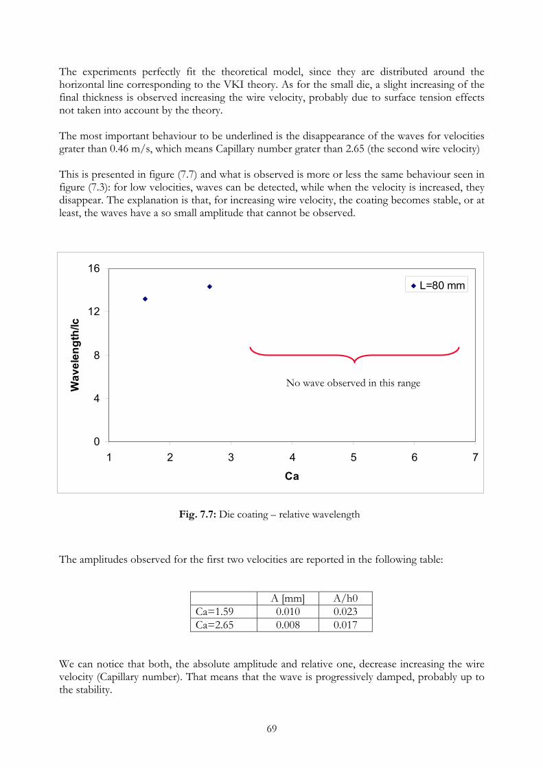
The experiments perfectly fit the theoretical model, since they are distributed around the horizontal line corresponding to the VKI theory. As for the small die, a slight increasing of the final thickness is observed increasing the wire velocity, probably due to surface tension effects not taken into account by the theory. The most important behaviour to be underlined is the disappearance of the waves for velocities grater than 0.46 m/s, which means Capillary number grater than 2.65 (the second wire velocity) This is presented in figure (7.7) and what is observed is more or less the same behaviour seen in figure (7.3): for low velocities, waves can be detected, while when the velocity is increased, they disappear. The explanation is that, for increasing wire velocity, the coating becomes stable, or at least, the waves have a so small amplitude that cannot be observed.
0
4
8
12
16
1 2 3 4 5 6 7
Ca
Wav
elen
gth/
lc
L=80 mm
No wave observed in this range
Fig. 7.7: Die coating – relative wavelength
The amplitudes observed for the first two velocities are reported in the following table:
A [mm] A/h0 Ca=1.59 0.010 0.023 Ca=2.65 0.008 0.017
We can notice that both, the absolute amplitude and relative one, decrease increasing the wire velocity (Capillary number). That means that the wave is progressively damped, probably up to the stability.
69

Since measurements at only one distance from the die have been carried out, it is not possible to say anything about the amplification factor. Unfortunately, during these preliminary tests with the big die, only one probe was available, so that no measure of wave velocity has been performed. Starting from this point, further and more detailed tests with the big die have been performed in order to check more carefully the evolution of the stability behaviour of the flow when the wire velocity is increased. For this reason, the following tests will be in the range of velocities between 0.28 m/s and 0.66 m/s: at low velocity, waves are expected, while for the last velocities a flat spectrum is supposed to be found. 7.3.1 Mean final thickness Several tests have been performed at different distances L from the die and using different distances D between the two probes. In figure (7.8) the mean final thickness observed in the experiments and computed by VKI theory are shown. As usual, dimensionless form is used.
0
0.2
0.4
0.6
0.8
1
1.5 2 2.5 3 3.5 4Ca
h0/r0
L=131, D=40L=57, D=116L=57, D=40VKI Theory
Fig. 7.8: Die coating – relative thickness
70

The observation is the same as seen in the previous die coating tests: the mean final thickness increases a little bit increasing the velocity, even if the theory predicts a constant value. This is due to the assumption made for the theoretical model. The experiments show a very good agreement with the theory and with the previous test. Comparing figure (7.8) with figure (7.6), we can see that the values of the final thickness for Capillary number smaller than 4 are all behind the predicted value, as shown in figure (7.6). This confirms the repeatability of the measurements. An important remark is that even if the distance from the die changes, the final thickness does not change, meaning that it is an asymptotic value. 7.3.2 Wave velocity Since for these experimental tests two laser probes were available, it was possible to measure the experimental wave velocity for the die coating and to compare it with the values predicted by Lin & Liu theory [8].
0
0.5
1
1.5
2
2.5
3
3.5
4
0 1 2 3Ca
Wav
e ve
loci
ty *
µ/ σ
Experiments L=131, D=40
Experiments L=57, D=116
Experiments2 L=57, D=40
Theory by Lin& Liu [8]
4
Fig. 7.9: Die coating – dimensionless wave velocity
In figure (7.9) the experimental wave velocity measured for different distances from the die and between the probes is compared with the theoretical one. As usual, the scale starts from zero in order to see the slope of the curve. The surprisingly conclusion is that the measured and predicted value are exactly the same. The experimental wave velocity has been obtained dividing the known distance between the two probes by the shifting time needed to observe the two signals matching.
71

The fact that the wave velocity obtained at different distances from the die and for different distances between the probes is always the same, confirms the repeatability of the measurements and the possibility to obtain an experimental value that should be very close to the real one. Wave velocities have been detected up to the last Capillary number, even if it is not sure that at the last velocities waves can exist: that is the reason why at high Ca the line is not continuous. This is not a problem, because when there are not waves, the velocity measured is simply the velocity of the liquid film at the interface. 7.3.3 Wavelength The main porpoise of these detailed experimental tests was to check what happens in the range of velocities between 0.28 m/s and 0.66 m/s, since a disappearance of waves was noticed in the preliminary tests. The study of the wavelength is the best instrument in order to detect the presence or absence of waves, since from the spectrum this information is immediately obtained. In figure (7.10) the relative wavelength is plotted versus the Capillary number, for different distances from the die and for different distances between the probes. The wavelengths observed are the same detected in the preliminary tests and what is found is that the relative amplitude increases for increasing Capillary number. Repeating the tests for the different distances from the die gives always the same behaviour as function of the wire velocity (Ca number).
12
13
14
15
16
1.5 2 2.5 3 3.5 4
Ca
Wav
elen
gth/
lc
L=131, D=40L=57, D=116L=57, D=4
Progressive wave disappearance
Fig. 7.10: Die coating – relative wavelength
72

For high Capillary number, the lines in figure (7.10) are no more continuous. This is due to the fact the as the velocity increases, the wavelength also increases, but the peaks detected from the power spectra become more and more smaller, so that for capillary number greater than 3.5 it is not possible to distinguish them from the noise present in the signal. This wave disappearance is better shown in figure (7.11). The power spectrum as function of the wavelength is considered for different capillary number in order to clarify the physical phenomena observed. Figure (7.22 - a) represents the typical wavelength detected at Ca=1.59: a very sharp and evident peak is observed at λ=27.8 mm, the rest, around it, is noise. Increasing the wire velocity ((figure 7.22 – b)), up to Ca=2.54, the peak moves to λ=29.4 mm, but its power is reduced of about 50% with respect to the previous case (a). This says that the wave amplitude corresponding to that wavelength decreases. For Ca=3.54, the wavelength λ=31.1 mm has a very small peak, which can still be distinguished from the noise, while in the last test, at Ca=3.77, only noise is found.
20 22 24 26 28 30 32 34 36 38 400
0.5
1
Wavelength [mm]
Pow
er sp
ectru
m
coat2
20 22 24 26 28 30 32 34 36 38 400
0.5
1
Wavelength [mm]
Pow
er sp
ectru
m
coat1
20 22 24 26 28 30 32 34 36 38 400
0.5
1
Wavelength [mm]
Pow
er sp
ectru
m
coat1
20 22 24 26 28 30 32 34 36 38 400
0.5
1
Wavelength [mm]
Pow
er sp
ectru
m
coat2
(b)(a)
(c) (d)
Fig. 7.11: Die coating – power spectra for different Capillary number: a) Ca=1.59. b) Ca=2.57. c) Ca=3.57. d) Ca=3.77
73

This progressive reduction of the instability, with wavelength disappearance, was already detected for the small die and in the preliminary tests for the big die. These more detailed tests made in order to check the behaviour of the instability with small increasing of wire velocity steps reveal that the phenomenon is dominated by a progressive damping when the velocity is increased. 7.3.4 Wave amplitude Since the waves are found up to the last 2-3 Capillary number tested, it is possible to obtain the behaviour of the amplitude for two different distances L from the die, as function of the velocity. In figure (7.12) the amplitude divided by the mean final thickness is presented for the case L=57 mm, D=116 mm, which means that the amplitudes at two different stations are available: L=173 mm and L=57 mm.
0
0.002
0.004
0.006
0.008
0.01
0.012
1.5 2 2.5 3 3.5 4
Ca
A/h
0
L=173 mmL= 57 mm
Fig. 7.12: Die coating – relative wave amplitude The first remark is that not appreciable difference is found in the amplitude at higher level compared to the one at lower level. This means that the coating is very close to the neutral stability since no amplification neither damping is observed. An interesting feature is that the amplitude, at both level, decreases when the velocity is increased, but for Capillary number greater than 2.5 a slight increasing with the velocity is observed. It is important to remember that only the value measured up to Ca=3 have a physical meaning, since above that threshold very small waves are observed and sometimes it is difficult to distinguish them from the noise.
74
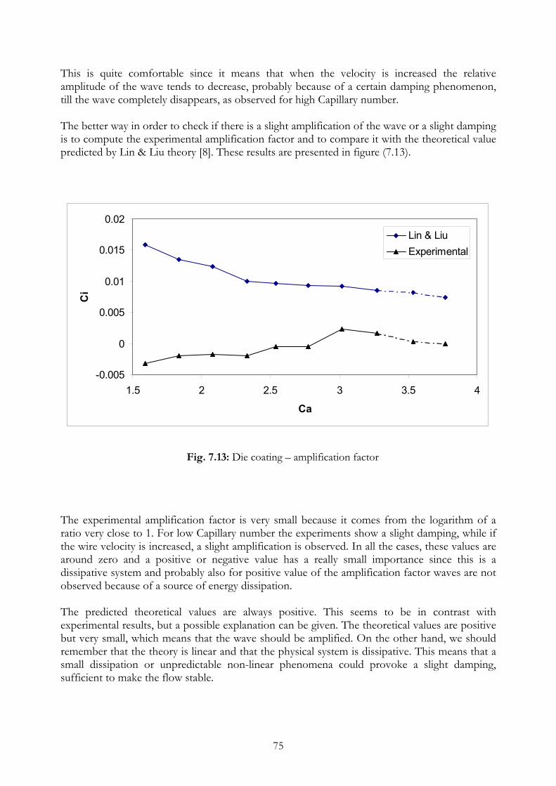
This is quite comfortable since it means that when the velocity is increased the relative amplitude of the wave tends to decrease, probably because of a certain damping phenomenon, till the wave completely disappears, as observed for high Capillary number. The better way in order to check if there is a slight amplification of the wave or a slight damping is to compute the experimental amplification factor and to compare it with the theoretical value predicted by Lin & Liu theory [8]. These results are presented in figure (7.13).
-0.005
0
0.005
0.01
0.015
0.02
1.5 2 2.5 3 3.5
Ca
Ci
Lin & LiuExperimental
4
Fig. 7.13: Die coating – amplification factor
The experimental amplification factor is very small because it comes from the logarithm of a ratio very close to 1. For low Capillary number the experiments show a slight damping, while if the wire velocity is increased, a slight amplification is observed. In all the cases, these values are around zero and a positive or negative value has a really small importance since this is a dissipative system and probably also for positive value of the amplification factor waves are not observed because of a source of energy dissipation. The predicted theoretical values are always positive. This seems to be in contrast with experimental results, but a possible explanation can be given. The theoretical values are positive but very small, which means that the wave should be amplified. On the other hand, we should remember that the theory is linear and that the physical system is dissipative. This means that a small dissipation or unpredictable non-linear phenomena could provoke a slight damping, sufficient to make the flow stable.
75

7.4 Horizontal die coating – die with geometrical defects In order to check the influence of geometrical defects on the stability of the liquid film. In the following table the fluid properties and geometrical characteristics are reported.
ρ 960 [kg/m3] Density µ 0.3 [Pa·s] Viscosity σ 0.02 [Pa/m] Surface tension r0 1·10-3 [m] Wire radius V 1 [m/s] Wire velocity
The wire velocity is kept constant and equal to 1 m/s for all the tests, the geometry of the die is similar to the one used in the vertical die coating, as shown in figure (7.14). The final part of the die can be changed so that different kind of defects can be reproduced.
changeable part
Fig. 7.14: Die with geometrical defects
Two geometrical conditions are considered: horizontal and vertical, depending on the position of the reference holes (see figure (7.15)). The laser plane is always vertical so that, the probe measures always the horizontal diameter. For each test conditions, 9 acquisitions at different sampling frequency are performed in order to be sure to follow the waves of different wavelength. In the following paragraphs, all the different cases are discussed reporting the results found.
76

(b) vertical position(a) horizontal position
Reference holes
Thickness measured
Wire
Fig. 7.15: Die with geometrical defect – reference figure
Die hole
7.4.1 Case 1 In this case, two parts compose the die and one is shifted with respect to the other for a displacement equal to 0.15 mm, so that they do not match exactly. The internal radius is 1.15 mm. The drawing of the die is reported in figure (7.16)
Fig. 7.16: Die with geometrical defect – case 1
77
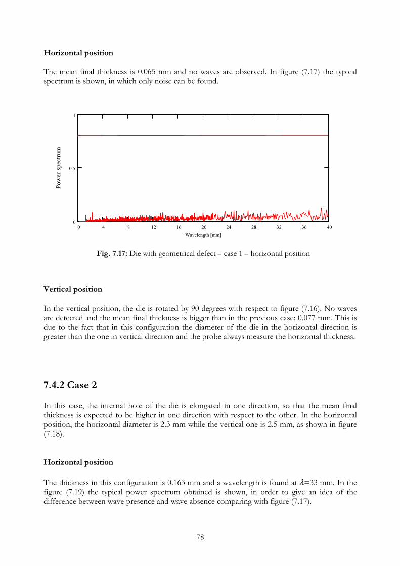
Horizontal position The mean final thickness is 0.065 mm and no waves are observed. In figure (7.17) the typical spectrum is shown, in which only noise can be found.
sim 8000 30000.. s_coat sim 0
0 4 8 12 16 20 24 28 32 36 400
0.5
1
Wavelength [mm]
Pow
er sp
ectru
m
Fig. 7.17: Die with geometrical defect – case 1 – horizontal position Vertical position In the vertical position, the die is rotated by 90 degrees with respect to figure (7.16). No waves are detected and the mean final thickness is bigger than in the previous case: 0.077 mm. This is due to the fact that in this configuration the diameter of the die in the horizontal direction is greater than the one in vertical direction and the probe always measure the horizontal thickness. 7.4.2 Case 2 In this case, the internal hole of the die is elongated in one direction, so that the mean final thickness is expected to be higher in one direction with respect to the other. In the horizontal position, the horizontal diameter is 2.3 mm while the vertical one is 2.5 mm, as shown in figure (7.18). Horizontal position The thickness in this configuration is 0.163 mm and a wavelength is found at λ=33 mm. In the figure (7.19) the typical power spectrum obtained is shown, in order to give an idea of the difference between wave presence and wave absence comparing with figure (7.17).
78
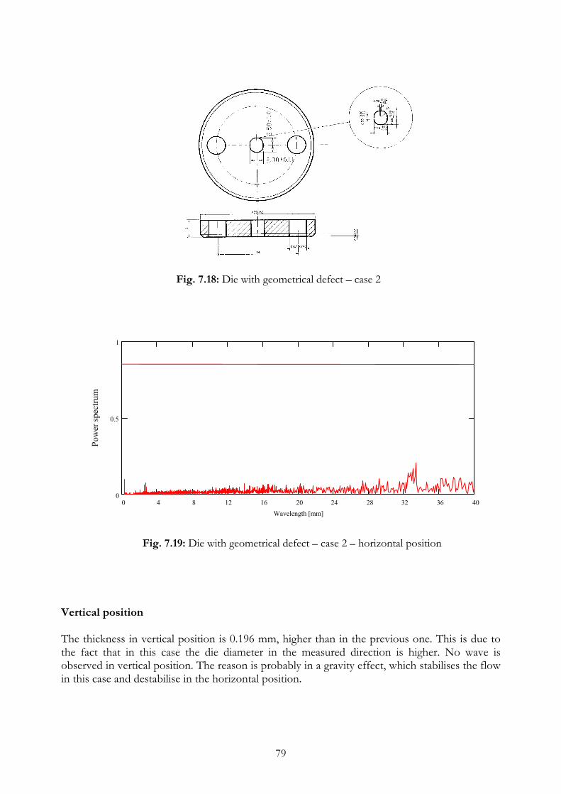
Fig. 7.18: Die with geometrical defect – case 2
c
0 4 8 12 16 20 24 28 32 36 400
0.5
1
Wavelength [mm]
Pow
er sp
ectru
m
Fig. 7.19: Die with geometrical defect – case 2 – horizontal position
Vertical position The thickness in vertical position is 0.196 mm, higher than in the previous one. This is due to the fact that in this case the die diameter in the measured direction is higher. No wave is observed in vertical position. The reason is probably in a gravity effect, which stabilises the flow in this case and destabilise in the horizontal position.
79
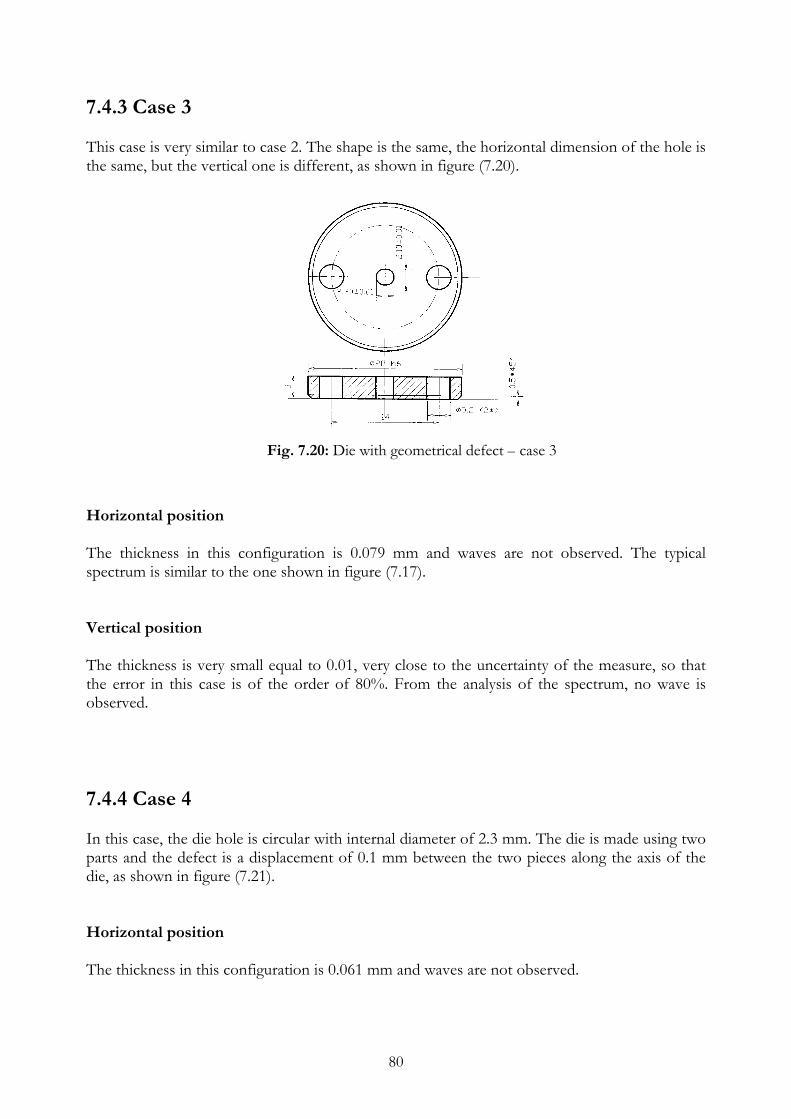
7.4.3 Case 3 This case is very similar to case 2. The shape is the same, the horizontal dimension of the hole is the same, but the vertical one is different, as shown in figure (7.20).
Fig. 7.20: Die with geometrical defect – case 3 Horizontal position The thickness in this configuration is 0.079 mm and waves are not observed. The typical spectrum is similar to the one shown in figure (7.17). Vertical position The thickness is very small equal to 0.01, very close to the uncertainty of the measure, so that the error in this case is of the order of 80%. From the analysis of the spectrum, no wave is observed. 7.4.4 Case 4 In this case, the die hole is circular with internal diameter of 2.3 mm. The die is made using two parts and the defect is a displacement of 0.1 mm between the two pieces along the axis of the die, as shown in figure (7.21). Horizontal position The thickness in this configuration is 0.061 mm and waves are not observed.
80

Fig. 7.21: Die with geometrical defect – case 4 Vertical position As in the horizontal case, the thickness is 0.06 mm and waves are not observed. This means that this kind of defect does not produce any difference in the final thickens and does not provoke any non-uniformity in the free surface. 7.4.5 Case 5 Case 5 is represented by the same defect as case 4, but the displacement is 0.3 mm instead of 0.1 mm. Horizontal position For this case a smaller diameter with respect to case 4 is found. It is 0.0445 mm instead of about 0.06. This is probably due to the effect of the surface tension at the exit of the die, so that is the defect is not negligible, a certain variation in the mean final thickness is found. Waves are not observed in this configuration Vertical position In this case, the mean final thickness is 0.061, which is close to the one found in case 4 and waves are not detected.
81
7.4.6 Case 6 – no defects In the last case, the same die but without geometrical defects is tested. Horizontal position The mean final thickness is 0.059 mm and in the power spectra it is impossible to observe any wave, as in figure (7.17). Vertical position The mean final thickness is 0.06 mm, which means the same observed for the horizontal case, and the spectra do not show any wave. 7.4.7 Conclusions about die with geometrical defects Only in one case waves have been observed and the characteristic wavelength is 33 mm. This situation correspond to the horizontal position in case 2, and the reason is probably a gravity effect that takes place because the thickness is greater than in all the other cases. From the tests performed, the main conclusion is that if the geometrical defect is small compared to the final coating thickness, it does not produce waves on the free surface. 7.5 Conclusions Since a lot has been said about the die coating instabilities, the main conclusions are hereafter summarised. The repeatability of the measure has been proved performing different tests for the same configuration and same conditions. For the vertical case, a small and a big die have been used, and almost the same behaviour has been found. The VKI theoretical model to predict the mean final thickness has been validated by the experimental measurements, which are in good agreement with the predicted values. A very
82

83
small increase of the coating thickness for increasing velocity, not theoretically predicted, is observed in the experiments. This difference is probably due to surface tension and inertia effects at high velocity that do not appear in the model. The wave velocity measured perfectly fit the theoretical curve from Lin & Liu [8]. The measurements have been performed for different distances between the probes and from the die, finding always the same results. For the wavelength, a typical value between 20 mm and 30 mm is observed. Only one wave is found for each velocity and the wavelength increases as the Capillary number rises. For high wire velocity, a progressive wave disappearance is observed: the peak in the power spectrum decreases, reducing its height so that it becomes impossible to distinguish it from the noise. The relative amplitude is almost constant with the Capillary number and there is not a big difference between the amplitude close to die and far from it. The amplification factor confirms this observation: the experimental one is very small and close to zero, meaning that the flow is almost neutrally stable. On the other hand, the theoretical value is slightly positive, meaning a small amplification, that is not probably observed because of a dissipation effect, not taken into account in the theory, which is enough in order to dump down the small amplification. In both cases, experimental and theoretical, the amplification factor goes to zero, and the waves disappear: the reason is probably in saturation phenomena as observed for vertical fibres. Die coating tests have been performed also in horizontal configuration for die with geometrical defects, in order to check their influence on the development of the coating and on the possible instability. In some cases waves have been observed, while in others no wavelength has been detected by the spectra. The reason is probably a gravity effect. In these horizontal configuration only one probe was available, so that nothing can be said about the wave velocity and amplification factor.

Chapter 8
Jet wiping results 8.1 Introduction For the annular jet wiping, several tests have been performed changing the possible parameters that influence the mean final thickness: the wire velocity, the stagnation pressure in the nozzle and the slot of the nozzle. The characteristics of the oil used, and all the other parameters are reported in the following table.
ρ 951 [kg/m3] Density µ 0.114 [Pa·s] Viscosity σ 0.02 [Pa/m] Surface tension r0 1·10-3 [m] Wire radius D 1.4·10-3 [m] Nozzle diameter s 0.5÷1·10-3 [m] Slot size P 0.5÷4 [kPa] Nozzle stagnation pressure V 0.25÷1.32 [m/s] Wire velocity
Two probes were available for these tests, which means that it was possible to measure the wave velocity and the amplification factor. In the following paragraphs all the results will be shown and discussed.
84

8.2 Mean final thickness Different tests have been carried out for different velocities and stagnation pressures, in order to have a clear idea of the behaviour of the thickness. In figure (8.1) the experimental data for all the pressures and all the velocities tested are reported. The complete comparison with the theory will be shown after, in order to have not too many curves on the same graph. The first remark is that increasing the velocity, the mean final thickness increases, for each stagnation pressure. The dependence on the velocity follows a curve that seems to be something like where V is the wire velocity in m/s, as suggested by previous works [4].
2.00 KVh =
00.10.20.30.40.50.60.70.80.9
0 0.2 0.4 0.6 0.8 1 1.2 1.4
V [m/s]
h0 [m
m]
Pn=.5 KPaPn=1 KpaPn=2 KPaPn=3 KPaPn=4 KPa
Fig. 8.1: Jet wiping coating – mean final thickness function of the wire velocity
For lower pressures, this behaviour is well followed for a large range of velocities, but a deviation is found for high velocities. This is particularly clear for the stagnation pressure equal to 0.5 kPa, which is the minimum pressure and for which the thickness is the maximum observed. Up to V=0.8 m/s the curvature of the curve followed by the data is negative, while for higher velocity the curvature becomes positive. This is probably due to the fact that the film coating exerts an influence on the pressure gradient. In the simple theoretical model called “Knife Model” [1] [2] [3] [4], the jet is supposed not to be influenced by the presence of the coating, while, when this thickness is high, there is probably an interaction.
85

00.10.20.30.40.50.60.70.80.9
0 0.5 1 1.5 2 2.5 3 3.5 4 4.5
Pn [KPa]
h0 [m
m]
V=0.25 m/s V=0.37 m/sV=0.47 m/s V=0.57 m/sV=0.68 m/s V=0.78 m/sV=0.89 m/s V=1 m/sV=1.1 m/s V=1.22 m/sV=1.32 m/s
Fig. 8.2: Jet wiping coating – mean final thickness function of the stagnation pressure
In figure (8.2) the final thickness in mm is plotted as function of the stagnation pressure Pn in the nozzle, for different wire velocities. The coating thickness decreases for increasing pressures, as expected, since the effect of the “air knife” becomes stronger. On the other hand, the thickness increases when the wire velocity increases, since a bigger amount of liquid is drown out from the liquid bath because of the viscous forces. The decreasing of the liquid thickness with the stagnation pressure is well fitted by a curve that behaves like as reported in [4]. 70
0.KPnh −=
After the presentation of the experimental results, it is possible to compare them with the theoretical values predicted by the “Knife Model” [3]. In figure (8.3) this comparison is presented. The maximum of the shear stress profile is set to zero, because its influence is negligible [1] [3] [4]. K is the constant that appears in the expression of the maximum of the pressure gradient:
sZPnK
dxxdp
MAX
=)( (8.1)
where K is a constant, Pn the stagnation pressure in the nozzle, s the slot in the nozzle and Z the distance between the wire and the nozzle. Two different values of K have been used, since in previous works they suggested 210 [1] and 0.72 [4]. In both cases, the theoretical values are very far from the experimental results and the error is at least 100% or more. This discrepancy was already outlined [1] [2] [3] [4], but they did not introduce any correction to the model. From figure (8.3) it is clear that a modification of the “Knife Model” is need in order to compare the mean final thickness found experimentally for the jet wiping.
86

Pn = 2 kPa
0
0.05
0.1
0.15
0.2
0.25
0.3
0.35
0 0.2 0.4 0.6 0.8 1 1.2 1.4V [m/s]
h0 [m
m]
ExperimentsKnife model K=14.14Knife model K=0.72
Fig. 8.3: Jet wiping coating – mean final thickness: comparison between
experimental data and “knife model” 8.2.1 Modification to the “Knife Model” Since a very big discrepancy is found between the experimental data and the predicted values by the theoretical “Knife Model” developed at VKI in the previous works, a modification of the model is introduced in the present one. The main assumption in the “Knife Model” is that the pressure gradient and the shear stress profiles are supposed unknown and the idea is to use a maximum value for both, in order to compute the mean final thickness after the jet wiping. The comparison with experimental results shown in figure (8.3), and what can be found in the previous works on annular jet wiping [1] [3] [4], show something like a shift between the experimental results and the predicted values. This is due to the fact that the maximum of the pressure gradient depends on different parameters, as described by equation (8.1), and the value of K is probably not correct. The main problem is, actually, the determination of K in the expression (8.1): in the previous works it has been evaluated by correlation performed on experiments carried out considering a jet impinging on a tube and found to be 210 [1] and then corrected to 0.72 [4]. Obviously, in these experiments there was no liquid coating on the tube and this is probably the main reason why the knife model does not work. In the real case the presence of the liquid film modifies the radius of the wire, which increases, and perhaps also the value of the maximum of the pressure gradient. If the radius is increased by the presence of the coating, the pressure profile is probably modified with respect to the case without coating, so that the assumption made for the “knife model” is no more valid.
87

The conclusion is that the correlation for the maximum of the pressure gradient is found performing experiments on a tube without coating, supposing that the presence of the film does not affect the pressure profile, while in the real case there is probably an interaction. Since it is practically impossible to measure the pressure profile or the maximum of the pressure gradient on a tube covered by a liquid film, the only way to make the model work is to refine the constant K. One possibility to do it is to change, for a certain velocity and a certain stagnation pressure, the value of K until the same experimental and theoretical value of the thickness is found. This procedure requires only one test, and the validity of the modified model can be checked in the other tests, for different velocities and stagnation pressure. Another possibility can be used in order to solve the problem. In previous works [4] and in the experiments performed in the present one as shown in figure (8.1) and (8.2), the final thickness is found to be a function of the wire velocity and stagnation pressure as:
2.00 Vh ≈ and (8.2) 7.0
0−≈ Pnh
The idea is first of all to find a value obtained for a fixed wire velocity V and stagnation pressure changing the value of until the experimental and theoretical value of the final thickness are the same. After this, the constant K can be made change with the wire velocity and the stagnation pressure in the following way:
0K 0V=
0PnP = 0K
7.02.0
0
00
=
PnPn
VVKK (8.3)
After this modification, the “Knife Model” will be called “Modified Knife Model”.
Pn=2 kPa
0
0.05
0.1
0.15
0.2
0.25
0 1 2 3 4 5 6 7 8Ca
h0/r0
ExperimentsK=constK=K(P,V)
Fig. 8.4: Jet wiping coating – mean final thickness: comparison between models
88

In figure (8.4) and (8.5) the results of the “Modified Knife Model” are presented, comparing the case in which K is kept constant and equal to , and the one in which K is function of the stagnation pressure and the velocity of the wire as relation (8.3)
0K
Ca=4.45
0
0.05
0.1
0.15
0.2
0.25
0.3
0.35
0 1 2 3 4 5P [kPa]
h0/r0
ExperimentsK=constK=K(P,V)
Fig. 8.5: Jet wiping coating – mean final thickness: comparison between models
The reference value of the wire velocity and pressure are 0.78 m/s (Ca=8.45) and 2 kPa. For constant pressure, equal to the reference one, the behaviour of the final thickness is presented in figure (8.4): if the K is kept constant, a bigger value than the experimental one is predicted for low velocity, while for high velocity a smaller than the observed one is predicted. If the constant is considered function of the velocity as in equation (8.3), the agreement between experiments and theoretical prediction is much better for a wide range of velocities (figure (8.4)). The only considerable difference is found for very high values of the Capillary number and it is probably due to the fact that the thickness is quite big and its presence can influence the maximum of the pressure gradient. In figure (8.5) the behaviour of the final thickness as function of the stagnation pressure, for the reference velocity, is shown. As the pressure increases, the mean thickness decreases, and if K is given by formula (8.3) there is a perfect agreement between experimental data and predicted values. Since when K is considered function of V and Pn very good agreement with experimental results is obtained, in the following comparisons K will be give by equation (8.3). With this modification of the program, much better results have been obtained, even if for very low pressure and very high velocity a small difference is still observed.
89

8.2.2 Validation of the “Modified Knife Model” In the following figures, a detailed comparison between experimental results and theoretical values predicted by the “Modified Knife Model” will be presented. In figure (8.6) the dependence of the mean final thickness on the Capillary number, for different stagnation pressure is shown. The worst case is for very low pressure and high Capillary number. This is due to the fact that the influence of the coating film on the pressure gradient, in that case, is the maximum because the thickness is the maximum possible. Since in the knife model this interaction is not taken into account, the discrepancy was expected. For very low pressure (figure (8.6) Pn=0.5 kPa), if the Capillary number is smaller than 4.5, a perfect agreement between the “Modified Knife Model” and the experimental results is found. As the pressure increases (figure (8.6) Pn=1 and Pn=3), the range of velocities in which the agreement is very good is extended to higher Capillary number. The best agreement for all the velocity range is found at Pn=3 kPa and Pn=4 kPa (figure (8.6)). The main reason is that at high pressure the thickness is smaller and its influence on the pressure distribution due to the jet is weaker.
90

91
Pn=0.5 kPa
0
0.2
0.4
0.6
0.8
1
0 1 2 3 4 5 6 7 8Ca
h0/r0
l
Pn=1 kPa
0
0.2
0.4
0.6
0 1 2 3 4 5 6 7 8Ca
h0/r0
l
Pn=2 kPa
0
0.2
0.4
0 1 2 3 4 5 6 7 8Ca
h0/r0
l
Pn=3 kPa
0
0.2
0 1 2 3 4 5 6 7 8Ca
h0/r0
l
Pn=4 kPa
0
0.2
0 1 2 3 4 5 6 7 8Ca
h0/r0
l
Experiments
Modified Knike ModeExperiments Modified Knife Model
Experiments
Modified Knike ModeExperiments Modified Knife Model
Experiments
Modified Knike ModeExperiments Modified Knife Model
Experiments
Modified Knike ModeExperiments Modified Knife Model
Experiments
Modified Knike ModeExperiments Modified Knife Model
Fig. 8.6: Jet wiping coating – mean final thickness:
comparison at different stagnation pressures

92
Ca=1.44
0
0.2
0 0.5 1 1.5 2 2.5 3 3.5 4 4.5Pn [kPa]
h0/r0
l
Ca=3.27
0
0.2
0.4
0 0.5 1 1.5 2 2.5 3 3.5 4 4.5Pn [kPa]
h0/r0
l
Ca=4.45
0
0.2
0.4
0 0.5 1 1.5 2 2.5 3 3.5 4 4.5Pn [kPa]
h0/r0
l
Ca=5.67
0
0.2
0.4
0.6
0 0.5 1 1.5 2 2.5 3 3.5 4 4.5Pn [kPa]
h0/r0
l
Ca=6.93
0
0.2
0.4
0.6
0.8
1
0 0.5 1 1.5 2 2.5 3 3.5 4 4.5Pn [kPa]
h0/r0
l
Experiments
Modified Knike ModeExperiments Modified Knife Model
Experiments
Modified Knike ModeExperiments Modified Knife Model
Experiments
Modified Knike ModeExperiments Modified Knife Model
Experiments
Modified Knike ModeExperiments Modified Knife Model
Experiments
Modified Knike ModeExperiments Modified Knife Model
Fig. 8.7: Jet wiping coating – mean final thickness:
comparison at different Capillary number
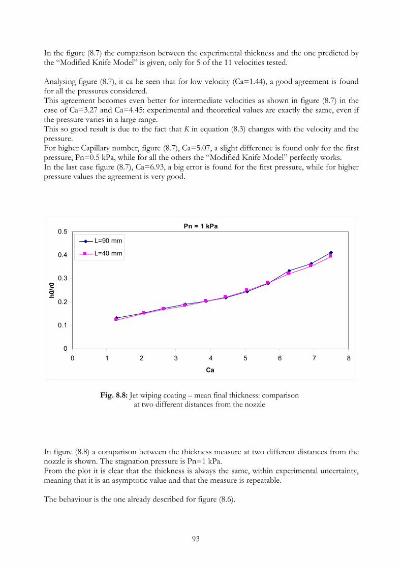
In the figure (8.7) the comparison between the experimental thickness and the one predicted by the “Modified Knife Model” is given, only for 5 of the 11 velocities tested. Analysing figure (8.7), it ca be seen that for low velocity (Ca=1.44), a good agreement is found for all the pressures considered. This agreement becomes even better for intermediate velocities as shown in figure (8.7) in the case of Ca=3.27 and Ca=4.45: experimental and theoretical values are exactly the same, even if the pressure varies in a large range. This so good result is due to the fact that K in equation (8.3) changes with the velocity and the pressure. For higher Capillary number, figure (8.7), Ca=5.07, a slight difference is found only for the first pressure, Pn=0.5 kPa, while for all the others the “Modified Knife Model” perfectly works. In the last case figure (8.7), Ca=6.93, a big error is found for the first pressure, while for higher pressure values the agreement is very good.
Pn = 1 kPa
0
0.1
0.2
0.3
0.4
0.5
0 1 2 3 4 5 6 7 8
Ca
h0/r0
L=90 mm
L=40 mm
Fig. 8.8: Jet wiping coating – mean final thickness: comparison
at two different distances from the nozzle In figure (8.8) a comparison between the thickness measure at two different distances from the nozzle is shown. The stagnation pressure is Pn=1 kPa. From the plot it is clear that the thickness is always the same, within experimental uncertainty, meaning that it is an asymptotic value and that the measure is repeatable. The behaviour is the one already described for figure (8.6).
93
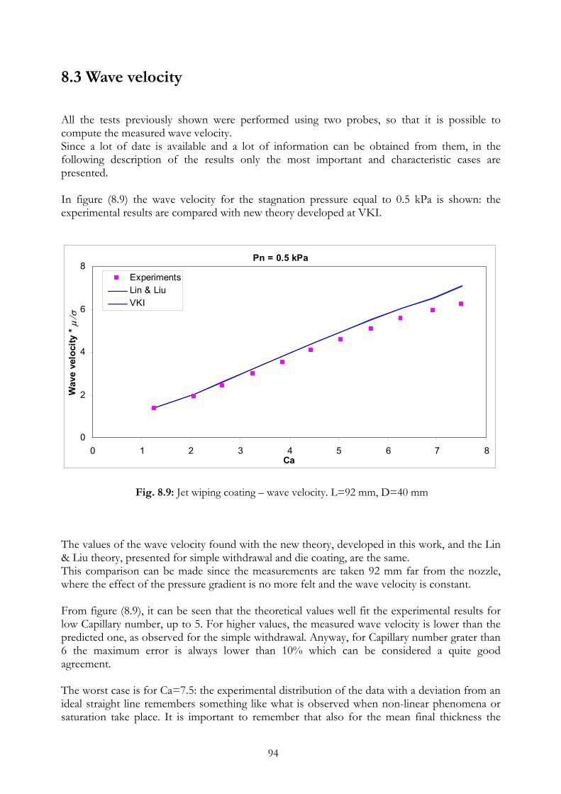
8.3 Wave velocity All the tests previously shown were performed using two probes, so that it is possible to compute the measured wave velocity. Since a lot of date is available and a lot of information can be obtained from them, in the following description of the results only the most important and characteristic cases are presented. In figure (8.9) the wave velocity for the stagnation pressure equal to 0.5 kPa is shown: the experimental results are compared with new theory developed at VKI.
Pn = 0.5 kPa
0
2
4
6
8
0 1 2 3 4 5 6 7 8Ca
Wav
e ve
loci
ty *
µ/σ
ExperimentsLin & LiuVKI
Fig. 8.9: Jet wiping coating – wave velocity. L=92 mm, D=40 mm The values of the wave velocity found with the new theory, developed in this work, and the Lin & Liu theory, presented for simple withdrawal and die coating, are the same. This comparison can be made since the measurements are taken 92 mm far from the nozzle, where the effect of the pressure gradient is no more felt and the wave velocity is constant. From figure (8.9), it can be seen that the theoretical values well fit the experimental results for low Capillary number, up to 5. For higher values, the measured wave velocity is lower than the predicted one, as observed for the simple withdrawal. Anyway, for Capillary number grater than 6 the maximum error is always lower than 10% which can be considered a quite good agreement. The worst case is for Ca=7.5: the experimental distribution of the data with a deviation from an ideal straight line remembers something like what is observed when non-linear phenomena or saturation take place. It is important to remember that also for the mean final thickness the
94

main discrepancy with theoretical prediction was found at high Capillary number and low pressure. Since tests have been performed for 5 different stagnation pressures and 11 velocities, it is possible to compare the different cases. In figure (8.10) the wave velocity for a higher stagnation pressure, 1 kPa, is presented. Two different tests were performed using different distances D between the two probes, and they are compared in the following plot.
Pn = 1 kPa
0
1
2
3
4
5
6
7
8
0 1 2 3 4 5 6 7Ca
Wav
e ve
loci
ty *
µ/σ
Experiments D=90
Experiments D=40
VKI
8
Fig. 8.10: Jet wiping coating – wave velocity. L=57 mm In both experiments the distance L of the first probe from the nozzle is 57 mm, while the distance D between the probes is 90 mm or 40 mm. From figure (8.10) it is evident that the wave velocity measured in the two tests is always the same and this is a good prove of the repeatability of the measure. The difference between theoretical predictions and experimental results is visible only for Capillary number greater than 5 and the maximum error in this range is no more than 10%. The dependence of the wave velocity on the pressure, for 4 different velocities, is summarised in figure (8.11). A very slight increasing of the wave velocity is observed as the stagnation pressure increases, and the only relevant increase is between 0.5 kPa and 1 kPa. For the other pressure, the value of the wave velocity can be considered constant. The comparison with the theory shows a very good agreement for low velocities, as observed in figure (8.10), but when the Capillary number rises, a bigger discrepancy is observed even if the relative error is always lower than 10%.
95
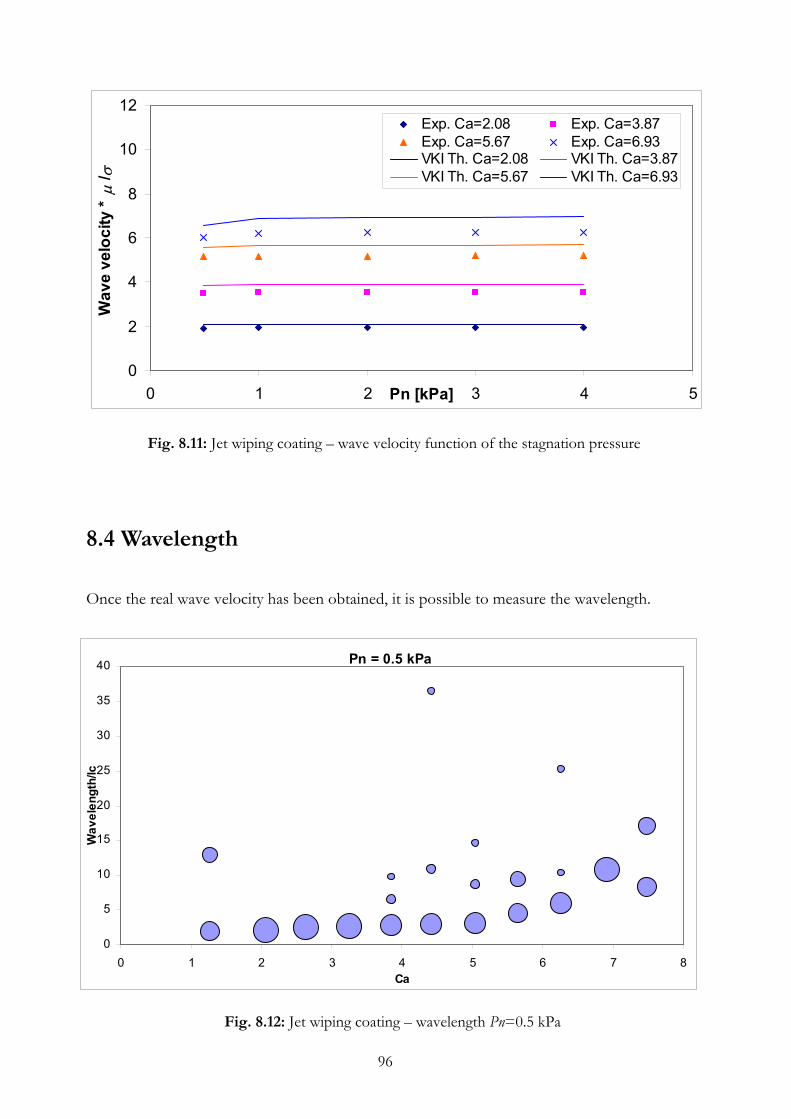
0
2
4
6
8
10
12
0 1 2 3 4 5Pn [kPa]
Wav
e ve
loci
ty *
µ/ σ
Exp. Ca=2.08 Exp. Ca=3.87Exp. Ca=5.67 Exp. Ca=6.93VKI Th. Ca=2.08 VKI Th. Ca=3.87VKI Th. Ca=5.67 VKI Th. Ca=6.93
Fig. 8.11: Jet wiping coating – wave velocity function of the stagnation pressure 8.4 Wavelength Once the real wave velocity has been obtained, it is possible to measure the wavelength.
Pn = 0.5 kPa
0
5
10
15
20
25
30
35
40
0 1 2 3 4 5 6 7Ca
Wav
elen
gth/
lc
8
Fig. 8.12: Jet wiping coating – wavelength Pn=0.5 kPa
96

In figure (8.12) the relative wavelength (the wavelength observed divided by the capillary length) is presented as function of the Capillary number for the lowest pressure, Pn=0.5 kPa. Since more than one wavelength for each test velocity is observed, a diagram as in the case of simple withdrawal is used. The first remark is that the relative wavelength increases when the Capillary number increases. For Ca<5 this phenomenon is not so strong: the relative wavelength increases very slowly and can be considered almost constant. This is not true for higher value of Ca: for the last 3 test velocities, figure (8.12), the rising of the wavelength is fast and reminds the apparently non-linear behaviour observed for the wave velocity. Since the capillary length is of the order of 2 mm, from the previous figure the dimensional wavelength can be deduced. It is of the order of 4 mm and this is the main difference observed between the jet wiping and all the other technique (simple withdrawal and die coating), in which the characteristic wavelength was of the order of 20-30 mm. An order of magnitude of difference can be important if non-uniformity in the final surface have to be avoided. At the first Capillary number, a peak is observed not only for low wavelength (at λ/lc=2) but also at λ/lc=13. When the velocity increases, the highest wavelength disappears for Ca in the range between 2 and 3.5. For Ca>3.5 other peaks are observed and their corresponding wavelength increases increasing the wire velocity. In figure (8.13) and (8.14) the wavelengths observed at higher pressure, 1 kPa, and different distances from the nozzle are shown. The main wavelengths are present in both cases and are always the same, so that we can say that the behaviour close to the nozzle or far from it is very similar. What changes between figure (8.13) and (8.14) is the disappearance or appearance of some peaks at higher wavelength for high Capillary number. As for low stagnation pressure, two peaks are found at the first Capillary number. Increasing the wire velocity only one wavelength is found up to Ca=4, and for Ca>4 usually more that a single wavelength is observed for each Capillary number. Comparing figure (8.13) and (8.14) with figure (8.12), the most evident difference is found at high Capillary number. The strongly non-linear behaviour observed at low pressure for Ca>6.5 is no more present and the growing in the wavelength is more gradual, without fast increasing.
97

Pn = 1 kPA
0
5
10
15
20
25
30
35
0 1 2 3 4 5 6 7 8Ca
Wav
elen
gth/
lc
Fig. 8.13: Jet wiping coating – wavelength L=97 mm
c
h/l
ngt
ele
Wav
Pn = 1 kPa
0
5
10
15
20
25
30
35
0 1 2 3 4 5 6 7 8Ca
Fig. 8.14: Jet wiping coating – wavelength L=147 mm
98
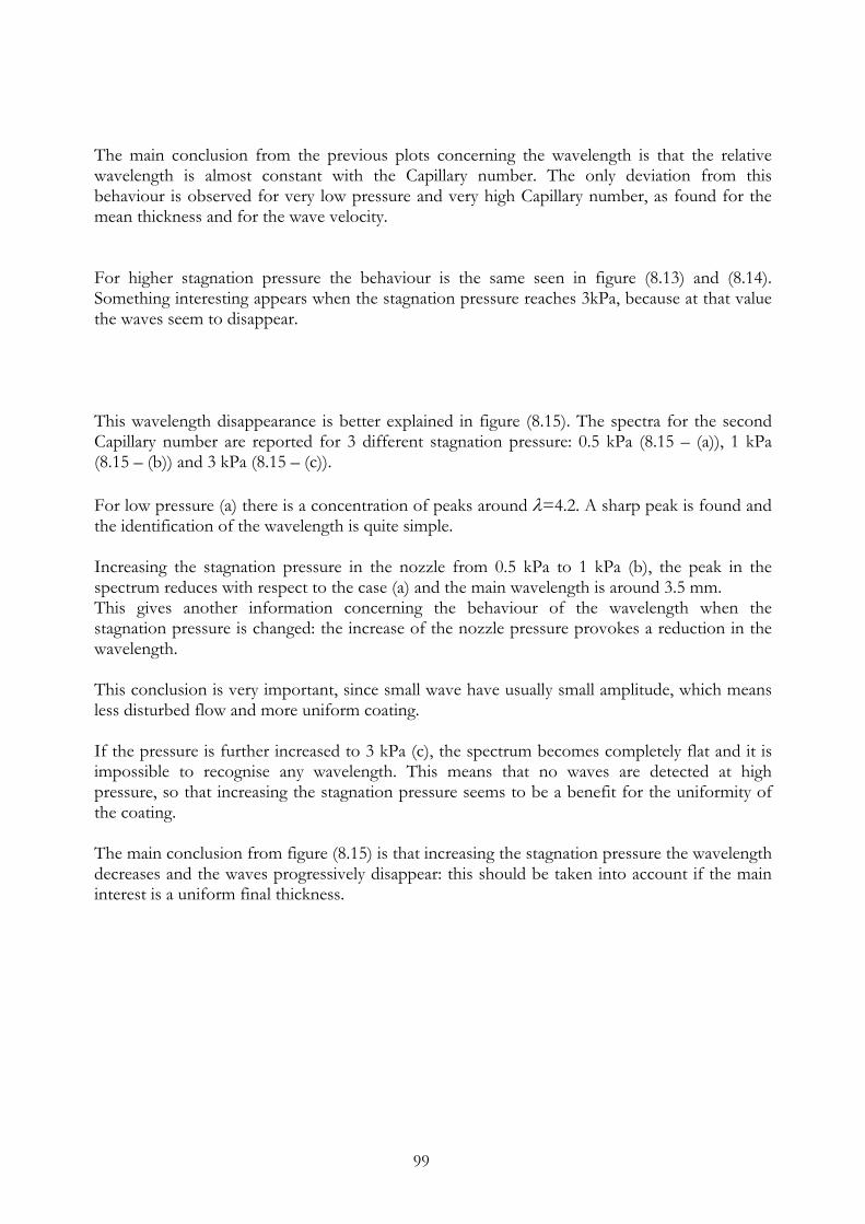
The main conclusion from the previous plots concerning the wavelength is that the relative wavelength is almost constant with the Capillary number. The only deviation from this behaviour is observed for very low pressure and very high Capillary number, as found for the mean thickness and for the wave velocity. For higher stagnation pressure the behaviour is the same seen in figure (8.13) and (8.14). Something interesting appears when the stagnation pressure reaches 3kPa, because at that value the waves seem to disappear. This wavelength disappearance is better explained in figure (8.15). The spectra for the second Capillary number are reported for 3 different stagnation pressure: 0.5 kPa (8.15 – (a)), 1 kPa (8.15 – (b)) and 3 kPa (8.15 – (c)). For low pressure (a) there is a concentration of peaks around λ=4.2. A sharp peak is found and the identification of the wavelength is quite simple. Increasing the stagnation pressure in the nozzle from 0.5 kPa to 1 kPa (b), the peak in the spectrum reduces with respect to the case (a) and the main wavelength is around 3.5 mm. This gives another information concerning the behaviour of the wavelength when the stagnation pressure is changed: the increase of the nozzle pressure provokes a reduction in the wavelength. This conclusion is very important, since small wave have usually small amplitude, which means less disturbed flow and more uniform coating. If the pressure is further increased to 3 kPa (c), the spectrum becomes completely flat and it is impossible to recognise any wavelength. This means that no waves are detected at high pressure, so that increasing the stagnation pressure seems to be a benefit for the uniformity of the coating. The main conclusion from figure (8.15) is that increasing the stagnation pressure the wavelength decreases and the waves progressively disappear: this should be taken into account if the main interest is a uniform final thickness.
99
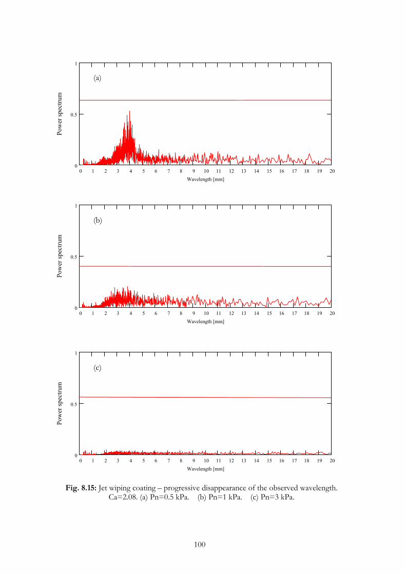
1 cont 1=
0 1 2 3 4 5 6 7 8 9 10 11 12 13 14 15 16 17 18 19 200
0.5
1
Wavelength [mm]
Pow
er sp
ectru
m
1 cont 1=
0 1 2 3 4 5 6 7 8 9 10 11 12 13 14 15 16 17 18 19 200
0.5
1
Wavelength [mm]
Pow
er sp
ectru
m1 cont 2=
0 1 2 3 4 5 6 7 8 9 10 11 12 13 14 15 16 17 18 19 200
0.5
1
Wavelength [mm]
Pow
er sp
ectru
m
(a)
(c)
(b)
Fig. 8.15: Jet wiping coating – progressive disappearance of the observed wavelength. Ca=2.08. (a) Pn=0.5 kPa. (b) Pn=1 kPa. (c) Pn=3 kPa.
100

To have a better idea of the behaviour of the wavelength when the pressure is increased, it is possible to plot the relative wavelength versus Pn.
0
1
23
4
5
6
78
9
10
0 0.5 1 1.5 2 2.5 3 3.5 4 4.5Pn [kPa]
Wav
elen
gth/
lc
Exp. Ca=2.08Exp. Ca=3.87Exp. Ca=5.67Exp. Ca=6.93
Wave disappearance
Fig. 8.16: Jet wiping coating – wavelength variation with the pressure From figure (8.16) is clear that the wavelength decreases when the stagnation pressure is increased. The strongest decreasing is observed when the pressure grows up from 0.5 kPa to 1 kPa. For high Capillary numbers this damping effect is more felt. For stagnation pressure greater than 2.5, and for each Capillary number, the waves disappear and from the spectra it is not possible to observe peaks anymore, as shown in figure (8.15). 8.5 Wave amplitude The observation of the wave amplitude is important because small relative amplitude means more uniform coating and because from the comparison between the measured amplitudes at two different stations it is possible to obtain information concerning the amplification or the damping of the waves. In figure (8.17) and (8.18) the relative amplitude for two different distances from the nozzle and for two different stagnation pressure is shown, in order to discuss the parameter that influence the amplitude of the wave.
101

Pn = 0.5 kPa
0
0.1
0.2
0.3
0.4
0.5
0.6
0 1 2 3 4 5 6 7Ca
A/h
0
L=132 mmL=92 mm
8
Fig. 8.17: Jet wiping coating – wave amplitude, Pn=0.5 kPa
Pn = 1 kPa
0
0.1
0.2
0.3
0.4
0.5
0.6
0 1 2 3 4 5 6 7 8Ca
A/h
0
L=134 mm
L=84 mm
Fig. 8.18: Jet wiping coating – wave amplitude, Pn=1 kPa
102

At low pressure, 0.5 kPa (figure (8.17)), the relative amplitude at higher distance from the nozzle is found to be smaller than the one closer to the nozzle. This means that a reduction in the amplitude is observed experimentally. The general trend of the relative amplitude is to increase for increasing velocity. The value, for amplitude measured at the lower station, is around 40-45% of the mean final thickness, while for the higher station is about 30-35%. If the stagnation pressure is increased to 1 kPa, the relative amplitude still increases with the Capillary number, and further from the nozzle the relative amplitude is still smaller than closer to it, as for Pn=0.5 kPa. A part from this general behaviour, some differences can be found comparing figure (8.17) and (8.18). First of all, at low Ca, the relative amplitude is smaller for higher pressures (8.17), while at higher Ca the behaviour is almost the same. For Pn=1 kPa, the relative amplitude goes from 20% to 50% and the difference between the closer and further station is smaller than for Pn=0.5. It is important to remember that even if the difference is smaller, it does not mean that the damping is higher, because the damping is related to the ratio between the amplitudes and not to their difference. An important remark is that for the jet wiping a very large relative amplitude have been found: it of the order of 40%. This implies that the linear theory with the asymptotic expansion developed in the frame of this work is no more valid, since the phenomenon is highly non-linear. One way to show the amplification or damping of the wave is to plot the amplification factor found in the experiments and computed by the theory: C
i
Pn = 0.5 kPa
-5
-4
-3
-2
-1
0
1
2
0 1 2 3 4 5 6 7 8Ca
-0.005
-0.004
-0.003
-0.002
-0.001
0
0.001
0.002
ExperimentsVKI theory
Fig. 8.19: Jet wiping coating – amplification factor, Pn=0.5 kPa
103
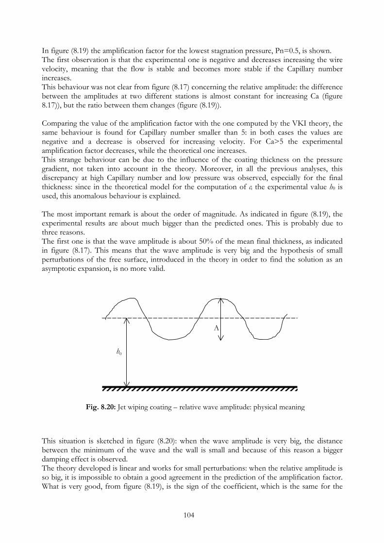
In figure (8.19) the amplification factor for the lowest stagnation pressure, Pn=0.5, is shown. The first observation is that the experimental one is negative and decreases increasing the wire velocity, meaning that the flow is stable and becomes more stable if the Capillary number increases. This behaviour was not clear from figure (8.17) concerning the relative amplitude: the difference between the amplitudes at two different stations is almost constant for increasing Ca (figure 8.17)), but the ratio between them changes (figure (8.19)). Comparing the value of the amplification factor with the one computed by the VKI theory, the same behaviour is found for Capillary number smaller than 5: in both cases the values are negative and a decrease is observed for increasing velocity. For Ca>5 the experimental amplification factor decreases, while the theoretical one increases. This strange behaviour can be due to the influence of the coating thickness on the pressure gradient, not taken into account in the theory. Moreover, in all the previous analyses, this discrepancy at high Capillary number and low pressure was observed, especially for the final thickness: since in the theoretical model for the computation of ci the experimental value h0 is used, this anomalous behaviour is explained. The most important remark is about the order of magnitude. As indicated in figure (8.19), the experimental results are about much bigger than the predicted ones. This is probably due to three reasons. The first one is that the wave amplitude is about 50% of the mean final thickness, as indicated in figure (8.17). This means that the wave amplitude is very big and the hypothesis of small perturbations of the free surface, introduced in the theory in order to find the solution as an asymptotic expansion, is no more valid.
A
h0
Fig. 8.20: Jet wiping coating – relative wave amplitude: physical meaning This situation is sketched in figure (8.20): when the wave amplitude is very big, the distance between the minimum of the wave and the wall is small and because of this reason a bigger damping effect is observed. The theory developed is linear and works for small perturbations: when the relative amplitude is so big, it is impossible to obtain a good agreement in the prediction of the amplification factor. What is very good, from figure (8.19), is the sign of the coefficient, which is the same for the
104

experiments and for the theory. Howhever, linear model cannot predict the amplitude but only the onset or offset of the instability, so that the prediction can be considered quite good. The second reason for the different order of magnitude could be the uncertainty. Since the typical value of the thickness in the jet wiping experiments is 0.2 mm, to obtain an amplification factor of the order of 10-3 as predicted by the theory, it is necessary to know the amplitude of the wave with the precision of micron. This is simply impossible since the spatial resolution of the probe is 5 µm and the uncertainty estimated for the amplitude is about 8 µm (chapter 5). The last reason is the fact that the predicted value of the amplification factor is the initial growth rate, while the measured one is the integral of this and that’s why its value is bigger. In figure (8.21) the amplification factor as function of the Capillary number for a higher stagnation pressure, Pn=1 kPa, is reported. ts
men
ri
pe
ex
Ci
Pn = 1 kPa
-2.5
-2
-1.5
-1
-0.5
0
0 2 4 6 8Ca
-0.005
-0.004
-0.003
-0.002
-0.001
0
Ci theory
ExperimentsVKI theory
Fig. 8.21: Jet wiping coating – amplification factor, Pn=1 kPa The amplification factor is negative and becomes more negative increasing the wire velocity, meaning that the flow becomes more and more stable when the Capillary number increases. This is predicted also by the theory, even if the order of magnitude is still different: the reasons are the same explained for the case at low stagnation pressure. A better agreement in the general behaviour, with respect to the case of low stagnation pressure, is found between the experiments and the theoretical predictions.
105

The conclusion about the wave amplitude as function of the wire velocity is that when the Capillary number is increased, the relative amplitude increases, but the amplification factor decreases. These to different behaviours are not in contrast, since the amplitude observed gives information only about the presence of the wave, but does not say anything about the stability or instability of the wave, which is expressed by the amplification factor. Up to this point, the relative amplitude has been considered as function of the Capillary number. If the influence of the stagnation pressure for fixed wire velocity (Ca number) is considered, the following plot is obtained:
0
0.1
0.2
0.3
0.4
0.5
0 0.5 1 1.5 2 2.5 3 3.5 4 4.Pn [kPa]
A/h0
Exp. Ca=2.08 Exp. Ca=3.87
Exp. Ca=5.67 Exp. Ca=6.93
Wave disappearance
5
Fig. 8.22: Jet wiping coating – relative amplitude From figure (8.22) it is clear that the relative amplitude decreases for increasing stagnation pressure. For Pn>2.5 waves are not observed anymore as described for the wavelength. The fact that the relative amplitude decreases for increasing stagnation pressure is positive, since uniform coating can be obtained changing the pressure in the nozzle. Finally, the amplification factor as function of the pressure, for a fixed Capillary number, can be plotted (figure 8.23). It is clear that increasing the stagnation pressure, the amplification factor increase, even if it remains always negative. This means that the flow becomes less stable.
106

Ca = 1.44
-1.20
-0.80
-0.40
0.00
0 0.05 0.1 0.15 0.2 0.25 0.3 0.35 0.4 0.45Pn [kPA]
Ci e
xper
imen
ts
-0.0024
-0.0016
-0.0008
0C
i Theory
ExperimentsVKI Theory
Wave disappearance
Fig. 8.23: Jet wiping coating – amplification factor 8.5.1 Relaxation One possible way to interpret the fact that when the time increases (or the space, in our case) the wave is damped, it is to consider the relaxation theory. We don’t derive the theory here, but just recall the final results:
WAVEVDh
AA
µλσπ
4
30
4
1
2
316ln =
(8.4)
where A2 and A1 are the amplitude respectively at lower and upper level, D the distance between the probes, VWAVE the measure wave velocity, σ and µ the surface tension and viscosity of the fluid, λ the wavelength and h0 the mean final thickness. In equation (8.4) the experimental data have been inserted and the left-hand side and right-hand side term have been plotted in figure (8.24). It is clear that for Ca<5.5 the agreement between LHS and RHS is good, which means that the relaxation theory can be used to explain the damping phenomenon observed in annular jet wiping. For higher vales of Ca there is less agreement and this is probably due to highly non-linear phenomena that occur in that range.
107
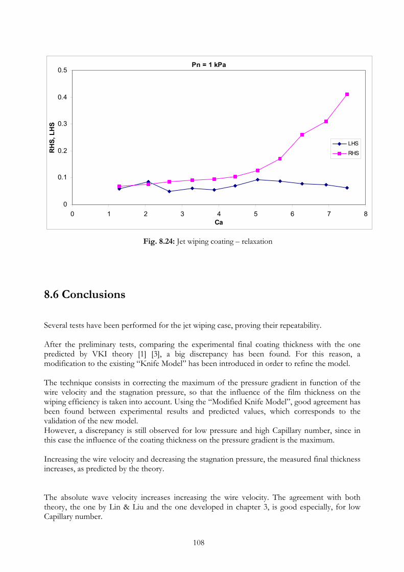
Pn = 1 kPa
0
0.1
0.2
0.3
0.4
0.5
0 1 2 3 4 5 6 7 8Ca
RH
S, L
HS
LHS
RHS
Fig. 8.24: Jet wiping coating – relaxation 8.6 Conclusions Several tests have been performed for the jet wiping case, proving their repeatability. After the preliminary tests, comparing the experimental final coating thickness with the one predicted by VKI theory [1] [3], a big discrepancy has been found. For this reason, a modification to the existing “Knife Model” has been introduced in order to refine the model. The technique consists in correcting the maximum of the pressure gradient in function of the wire velocity and the stagnation pressure, so that the influence of the film thickness on the wiping efficiency is taken into account. Using the “Modified Knife Model”, good agreement has been found between experimental results and predicted values, which corresponds to the validation of the new model. However, a discrepancy is still observed for low pressure and high Capillary number, since in this case the influence of the coating thickness on the pressure gradient is the maximum. Increasing the wire velocity and decreasing the stagnation pressure, the measured final thickness increases, as predicted by the theory. The absolute wave velocity increases increasing the wire velocity. The agreement with both theory, the one by Lin & Liu and the one developed in chapter 3, is good especially, for low Capillary number.
108

109
The wave velocity shows a very weak dependence on the stagnation pressure, since if the last is increased, the wave velocity remains almost constant. For the wavelength, it has been observed that increasing the wire velocity, the relative wavelength increases very slowly. At low Capillary number, two waves are found, while for mean values of Ca only one is present. For high Capillary number, again, more than one peak is detected in the spectrum. A big difference in the value of the typical wavelength is found with respect to the case of simple withdrawal or die coating. For jet wiping, the typical wavelength is 4 mm, one order of magnitude smaller. Changing the distance from the nozzle, almost the same wavelengths are observed. The dependence of the wavelength on the stagnation pressure shows a disappearance of the peaks in the spectra as the pressure is increased. This is probably due to the fact that at high pressure the thickness is smaller and the film more stable. For the observed waves, the wavelength decreases increasing the pressure. This is a very useful conclusion if the uniformity of the coating is a strong constrain. Increasing the stagnation pressure smaller waves are observed, up to the totally disappearance. Finally, the wave amplitude increases increasing the Capillary number. The surprisingly observation is that the relative amplitude, compared to the mean final thickness, is about 40%. This means that the linear theory can not be applied anymore, since the hypotheses are not satisfied. For this reason, the experimental amplification factor is orders of magnitude different from the theoretical one. Experimentally, a stronger damping is observed than the predicted one. One possible cause could be the damping effect due to the presence of the wall. However, the sign of ci is the same and also its behaviour with the Capillary number. Another possible explanation for the difference in the order of magnitude is the fact that the one predicted by the theory is the initial growth rate, while the measured one is an integral in space of the previous. Increasing the stagnation pressure, the wave amplitude decreases up to the totally disappearance of the wave. This is again a good result for the applications, since a more uniform coating can be obtained increasing the stagnation pressure.

Chapter 9
Conclusions 9.1 Conclusions of the project The instability behaviour of liquid film in wire coating process has been studied in this project. The motivations of such a research arise from the industrial field: waves are observed during the industrial coating process but in most of the cases they are not desired since a non-uniform final thickness is obtained. An overview of the problem is given in the first chapter, explaining the origin and the objectives of the project. The main goal was a detailed analysis of the characteristics of the waves observed in three main wire coating techniques: simple withdrawal, die coating and annular jet wiping coating. This means that the mean final thickness, the wave velocity, the wavelength, the wave amplitude and the amplification factor were the quantities to be measured in each case, in order to draw conclusions on the stable or unstable behaviour of the waves. A brief review of the three coating techniques investigated is presented in chapter two, describing the process and the modelling equations. For each case, the basic flow is solved, in order to compute the liquid flux and the final mean thickness. Previous models developed at VKI are described since they have been used for the comparison with the experimental results. In chapter three, a detailed literature search on the problem is presented. Since this work is the first at VKI concerning the liquid film instabilities of wire coatings, it was necessary to acquire the appropriate background concerning instability behaviour of thin liquid layers on wires or cylinders. Something has been found in literature about the case of a wire that moves with a certain velocity drawing a certain amount of liquid. In this case, the boundary conditions for the basic
110

flow impose a pressure equal to the atmospheric one at the interface liquid-air. Because of this reason, this theory can be applied only for the simple withdrawal, and for the die coating. For the annular jet wiping a new theoretical model has been developed in the frame of this project. This was necessary since in the jet wiping a pressure gradient and a shear stress profile due to the jet are imposed as boundary conditions at the free liquid surface. In developing the new model, the steps found in literature for the planar jet wiping have been combined with the steps followed for the axisymmetric case without pressure gradient. An expression for the wave velocity and the amplification factor has been found. The experimental set-up and the measurement technique are presented in chapter four. The experiments have been performed using GALFIN facility. A completely new measurement technique and data processing have been introduced and developed in this project for the study of the instability. The existing CCD camera and digital image processing has been replaced by a laser sheet probe in order to be able to observe both long and short waves, which require respectively a big investigation window and a small one. The high acquisition frequency of the laser sheet probe guarantees the possibility to follow the short waves. The original signal obtained by the probe is then processed in order to determine the presence or absence of the waves and their characteristics. A data processing program has been developed for this reason and implemented in Mathcad. The outputs of the program are the mean final thickness, the wave velocity, the wavelength and the wave amplitude and the amplification factor Since the wave velocity has to be computed, two identical laser sheet probes have been used: knowing the time required by the wave in order to go from the first probe to the second one and the distance between the two probes, the wave velocity is computed. The wavelength is determined looking at the power spectra and the amplitude computing the standard deviation of the reconstructed signal having only the investigated wavelength. The uncertainty analysis is performed in chapter five for the measured quantities. The uncertainty in the main parameter, which is the thickness as function of time, due to the probe is about 8 µm. The results obtained from simple withdrawal experiments are presented and discussed in chapter six. For the mean final thickness the VKI model has been validated: the experimental data and the predicted values are found in good agreement. The wave velocity measured for different distances between the probes and for different distances from the liquid bath is compared with the theoretical values, finding that the measured wave velocity is always slightly lower than the predicted one. The maximum error, within 10%, is observed for high wire velocity.
111
The wavelength analysis reveals the presence of more than a single wave for a fixed wire velocity. At low Capillary number the typical wavelength is 20-30 mm, while when, the wire velocity is increased, longer waves are observed with characteristic wavelength of 80-90 mm. Looking at the spectra, an energy transfer from low to high wavelength is observed, since the relative weight of the peaks changes increasing the wire velocity. Finally, the amplitude measured closer to the liquid bath is smaller than the one measured further from the liquid bath: this means that amplification is found and the flow is unstable. This is confirmed by the amplification factor computed from the experiments and compared with the one predicted by the theory. It is always positive, and for increasing velocity it decreases, going to zero, meaning that the instability is reduced when the wire velocity is increased. The die coating tests are presented and discussed in chapter seven. For the vertical die coating, two different sizes of the die have been used, finding always the same behaviour. The experimental final thickness is in agreement with the VKI theory, which predicts that the thickness is constant for increasing velocity. A very small increase of the coating thickness, not theoretically predicted, is observed in the experiments. This difference is probably due to surface tension and inertia effects at high velocity that do not appear in the model. For the wave velocity, a perfect agreement with the theory is found and the predicted curve perfectly fits the experimental data. The measures have been performed for different distances between the probes and from the die, finding always the same results. For the wavelength, a typical value between 20 mm and 30 mm is found. Only one wave is observed for each velocity and the wavelength increases, as the Capillary number rises. For high wire velocity, a progressive wave disappearance is observed: the peak in the power spectrum decreases reducing its height so that it becomes impossible to distinguish it from the noise. The relative amplitude is almost constant with the Capillary number and there is not a big difference between the amplitude close to die and far from it. The amplification factor confirms this observation: the experimental one is very small and close to zero, meaning that the flow is almost neutrally stable. On the other hand, the theoretical value is slightly positive, meaning a small amplification, that is not probably observed because of a dissipation effect, not taken into account in the theory, which is enough in order to damp down the small amplification. In both cases, experimental and theoretical, the amplification factor goes to zero, and the waves disappear: the reason is probably in saturation phenomena as observed for vertical fibres. Other tests have been performed in horizontal configuration for die with geometrical defects, in order to check the influence of them on the development of the coating. In some cases waves have been observed, while in others no wavelength has been detected by the spectra. The reason is probably in gravity effects. In these horizontal configuration only one probe was available, so that nothing can be said about the wave velocity and amplification factor.
112

The results from jet wiping tests are presented and discussed in chapter eight. For the mean final thickness, a modification to the existing “Knife Model” has been introduced in order to refine the model. The technique consists in correcting the maximum of the pressure gradient in function of the wire velocity and the stagnation pressure, in order to take into account the influence of the film thickness on the wiping efficiency. In this way, good agreement is found between experimental results and predicted values. However, a discrepancy is still observed for low pressure and high Capillary number, since in this case the influence of the coating thickness on the pressure gradient is the maximum. Increasing the wire velocity and decreasing the stagnation pressure, the measured final thickness increases, as predicted by the theory. The absolute wave velocity increases increasing the wire velocity. The agreement with the one by Lin & Liu and the one developed in chapter 3, is good especially, for low Capillary number. The wave velocity shows a very weak dependence on the stagnation pressure. For the wavelength, increasing the wire velocity, the relative wavelength increases very slowly. At low Capillary number, two waves are found, while for mean values of Ca only one is present. For high Capillary number, again, more than one peak is detected in the spectrum. A big difference in the value of the typical wavelength is found with respect to the case of simple withdrawal or die coating. For jet wiping, the typical wavelength is 2-3 mm, one order of magnitude smaller. Changing the distance from the nozzle, almost the same wavelengths are observed. The dependence of the wavelength on the stagnation pressure shows a disappearance of the peaks in the spectra as the pressure is increased. This is probably due to the fact that at high pressure the thickness is smaller and the film more stable. For the observed waves, the wavelength decreases increasing the pressure. This is a very useful conclusion if the uniformity of the coating is a strong constrain. Increasing the stagnation pressure smaller waves are observed, up to the totally disappearance. Finally, the wave amplitude increases increasing the Capillary number. The surprisingly observation is that the relative amplitude, compared to the mean final thickness, is about 40%. This means that the linear theory can not be applied anymore, since the hypotheses are not satisfied. For this reason, the experimental amplification factor is orders of magnitude different from the theoretical one. Experimentally, a stronger damping is observed than the predicted one. One possible cause could be the damping effect due to the presence of the wall. However, the sign of ci is the same and also its behaviour with the Capillary number. Another possible explanation for the difference in the order of magnitude is the fact that the one predicted by the theory is the initial growth rate, while the measured one is an integral in space of the previous.
113

114
Increasing the stagnation pressure, the wave amplitude decreases up to the totally disappearance of the wave. This is again a good result for the applications, since a more uniform coating can be obtained increasing the stagnation pressure. The relaxation theory is finally proposed since it explains the wave behaviour for low Capillary number. 9.2 Further work From the conclusion of the present work, further research can be suggested, in both experimental and theoretical fields. Experimental work. Since from the experimental results it has been found that the wavelength and wave amplitude depend on certain parameters, further experimental investigation could help in better understanding this dependence. For example, in the jet wiping case, increasing the stagnation pressure, the waves disappear. Unfortunately, the mean final thickness changes. If a certain final thickness is desired, it can be obtained increasing the stagnation pressure and increasing the internal diameter of the nozzle, in order to keep h0 constant and to reach a higher Pn. For this reason, further tests are needed changing the geometrical characteristics of the nozzle in jet wiping, like the slot or the internal diameter. Another possibility is to change the fluid properties and the radius of the wire, in order to obtain more data for further comparisons. Theoretical work. From the comparison between experiments and theoretical prediction concerning the instability behaviour, it has been found that the order of magnitude of the observed amplification factor is different from the theoretical one. This is due to the fact that the theory is linear, but in the real case this hypothesis is not always satisfied. For this reason, a non-linear theory or a non-linear correction to the theory is needed in order to predict something about the behaviour of the amplitude. The Landau equation [24] could be used for this porpoise. Finally, since a first attempt has give good agreement between theory and experiments, the relaxation theory is proposed as possible way to explain the wave behaviour.
References [1] Anthoine J., Annular Jet Wiping. Project Report 1996-02, von Karman Institute for Fluid
Dynamics, June 1996. [2] Laguna C., Numerical Investigation of Annular Jet Wiping. Stagiaire Report 1997-05, von Karman
Institute for Fluid Dynamics, November 1996. [3] Parrelada Perez N., Annular Jet Wiping. Project Report 1997-20, von Karman Institute for Fluid
Dynamics, June 1997. [4] Passelecq L., Annular Jet Wiping. Stagiaire Report 1997-98, von Karman Institute for Fluid
Dynamics. [5] Kistler S., Schweizer P., Liquid Film Coating: Scientific Principles and Their Technological Implications.
Chapman-Hall, 1997. [6] Benkeira H., Thin Film Coating. Royal Society of Chemistry, 1993. [7] Cohen E., Gutoff E., Modern Coating and Drying Technology. VCH, 1992. [8] Lin S. P., Liu W. C., Instability of Film Coating of Wires and Tubes, AIChE J., 1975 21, No. 4 775-
782. [9] Homsy G. M., Geyling F. T., A Note on Instabilities in Rapid Coating of Cylinders, AIChE J., 1977
23, No. 4 587-590. [10] Tu C. V., Coating Film Instability in the Jet Stripping Process, International Symposium on
Mechanics of Thin-Film Coating, New Orleans, 1988. [11] Tu C. V., Ellen C. H., Stability of Liquid Coating in the Jet Stripping Process, Research & Tecnology
Centre, BHP Coated Products Division [12] Krantz W. B., Zollard R. L., The Linear Hydrodynamic Stability of Film Flow Down a Vertical
Cylinder, AIChE J., 1976 22, No. 5 930-934. [13] Atherton R. W., Homsy G. M., On the Derivation of Evolution Equations for Interfacial Waves,
Chemical Engineering Communications, 1976 2, 57-77. [14] Patrick J. S., Zollard R. L., The Equivalence of Spatial and Temporal Formulations for the Linear
Stability of Falling Film Flow, AIChE J., 1976 22, No. 5 234-237.
115

[15] Gutfinger C., Chiu H., An Experimental Study of Continuous Free Withdrawal of Wires from Newtonian
Fluids ,. [16] Atherton R. W., Homsy G. M., A Note on Wave Inception in Film Flow, Chemical Engineering
Journal, 1973 6, 273-275. [17] Simon L. G., The Instability of an Annular Thread of Fluid,. [18] Quere D., Thin Films Flowing on Vertical Fibers, Europhysics Letters, 1990 13 (8), 721-726. [19] Newhouse L. A., Pozrikidis C., The Capillary Instability of Annular Layers and Liquid Threads, J.
Fluid Mech., 1992 242, 193-209. [20] Frenkel A. L., Babchin A. J., Levich B. G., Shlang T., Sivashinsky G. I., Annular Flows Can Keep
Unstable Films from Breakup: Nonlinear Saturation of Capillary Instability, Journal of Colloid and Interface Science, 1987 115 (1), 225-233.
[21] Mashayek F., Ashgriz N., Instability of Liquid Coatings on Cylindrical Surfaces, Phys. Fluids, 1995 7
(9), 2143-2153. [22] Kalliadasis S., Chang H. C., Drop Formation during Coating of Vertical Fibres, J. Fluid Mech., 1994
261 (1), 135-168. [23] Kerchman V. I., Frenkel A. L., Interactions of Coherent Structures in a Film Flow: Simulations of a
Highly Nonlinear Evolution Equation, Theor. Comput. Fluid Dynamics, 1994 6, 235-254. [24] Euromech 367, Fluid Mechanics of Coating Processes, 22-25 July 1997, Université Louis Pasteur,
Strasbourg, France. [25] Drazin P. G., Reid W. H., Hydrodynamic stability, Cambridge University Press, 1981.
116

Appendix
117

Data processing program forwire coating instabilities
Input parameters
r 0 1 10 3. Wire radius [m]
Liquid density [kg/m3]ρ 951
Liquid viscosity [N/m]µ .114
Gravity [m/s2]g 9.81
File nameName "acq0002.dat"
V .2254 Velocity of the wire
f sampl 500 Sampling frequency
N 15000 Number of samples to be consdered
Data processing
X READPRN Name( )
X1 X 0< > X2 X 1< >
T Nf sampl
T 30= Total time of the test [s]
i 0 N 1..
ti i TN 1. Time scale [s]
Space scale [mm]xi 1000 V. ti
.
d1i
X1i
1000.5007( ). 5.037 2.086
2Transformation in diameter [mm]
d2i
X2i
1000.5007( ). 5.037 2.086
2Transformation in diameter [mm]
118

s_coat1 cfft d1( ) s_coat1 0 0 l_s length s_coat1( ) s_coat2 cfft d2( ) s_coat2 0 0
k 0 length s_coat1( ) 1.. k 0 length s_coat2( ) 1..
fk kf sampl
N. fk k
f samplN
.
j 0 length s_coat1( ) 1..
d_m1 mean d1( ) d_m1 0.721= d_m2 mean d2( ) d_m2 0.669=
s1 stdev d1( ) s2 stdev d2( )
s_abs1 i s_coat1 i s_abs2 i s_coat2 i
max_s1 max s_abs1( ) max_s2 max s_abs2( )
shift d_m1 d_m2
0 1 2 3 4 5 6 70.6
0.7
0.8
0.9
HighLow
Evolution in time
t [s]
diam
eter
[mm
]
h 0 d_m1 10 3.
Homsy and Geylin
ξh 0 r 0
r 0ξ 1.721=
Toρ g. r 0
2.
µ V.To 0.363=
c r 1 To 1 ξ2
2ξ
2 ln ξ( ).. c r 0.772=
V1 V c r. V1 0.174=
119
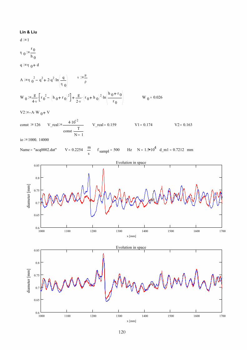
Lin & Liu
d 1
η 0r 0h 0
q η 0 d
νµ
ρA η 02 q2 2 q2. ln q
η 0.
W 0g
4 ν.r 0
2 h 0 r 02. g
2 ν.r 0 h 0
2. lnh 0 r 0
r 0. W 0 0.026=
V2 A W 0. V
const 126 V_real 4 10 2.
const TN 1.
V_real 0.159= V1 0.174= V2 0.163=
io 1000 14000..
Name "acq0002.dat"= V 0.2254=ms
f sampl 500= Hz N 1.5 104= d_m1 0.7212= mm
1000 1100 1200 1300 1400 1500 1600 17000.6
0.65
0.7
0.75
0.8
0.85Evolution in space
x [mm]
diam
eter
[mm
]
1000 1100 1200 1300 1400 1500 1600 17000.6
0.65
0.7
0.75
0.8
0.85Evolution in space
x [mm]
diam
eter
[mm
]
120

121
0 2.5 5 7.5 10 12.5 15 17.5 20 22.5 25 27.5 30 32.5 35 37.5 40 42.5 45 47.5 500
0.5
1
High
Power spectrum
frequency [Hz]
pow
er sp
ectru
m
0 6 12 18 24 30 36 42 48 54 60 66 72 78 84 90 96 102 108 114 1200
0.5
1
HighLow
Wave length
Wavelength [mm]
Pow
er sp
ectru
m
lower_limit 1 upper_limit 250 lower_window 1 upper_window 40
lw_w ceil 1000 V_real. Nf sampl lower_window.. up_w floor 1000 V_real. N
f sampl upper_window..
up_w 119 lw_w 4.762 103=
filterk 0 one_spectr1 up_w lw_w.. filterone_spectr1 1 one_spectr2 N lw_w( ) N up_w( ).. filterone_spectr2 1
s_coat_filter k s_coat1 k filterk. d_filter icfft s_coat_filter( ) dm_filter mean d_filter( ) A1 2 2. stdev d_filter( ).
=

A1
2 2.0.014= A1 0.0396=
filterk 0 one_spectr1 up_w lw_w.. filterone_spectr1 1 one_spectr2 N lw_w( ) N up_w( ).. filterone_spectr2 1
s_coat_filter k s_coat2 k filterk. d_filter icfft s_coat_filter( ) dm_filter mean d_filter( ) A2 2 2. stdev d_filter( ).
A2
2 2.0.013= A2 0.0377=
CI V_real
9 10 2.ln A1
A2. CI 0.085=
0 50 100 150 200 250 3000.1
0
0.1
0.2
0 5 10 150
0.1
0.2
0.3
0.4
122

Theoretical predictions
r 0 1 10 3.
V .9947
λ 2.5 10 3.
h 0 .106 10 3.
σ .0209
ρ 951
µ .114
g 9.81
T σ
ξh 0 r 0
r 0ξ 1.106=
Toρ g. r 0
2.
µ V.To 0.082=
Homsy and Geylin
ξh 0 r 0
r 0ξ 1.106=
Toρ g. r 0
2.
µ V.To 0.082=
c r 1 To 1 ξ2
2ξ
2 ln ξ( ).. c r 0.999=
V1 V c r. V1 0.994=
123

Lin & Liu
d 1
η 0r 0h 0
q η 0 d
νµ
ρA η 02 q2 2 q2. ln q
η 0.
W 0g
4 ν.r 0
2 h 0 r 02. g
2 ν.r 0 h 0
2. lnh 0 r 0
r 0. W 0 4.756 10 4=
V2 A W 0. V
µ2 π. h 0.
λ
ReW 0 h 0.
ν
We T
ρ g. h 02.
q η 0 d
Qη 0
η 0 d
B 12
q6. ln Q( )( )3. 5 q4. η 02 q2. ln Q( )( )2
8. q2 η 0
2. 17 q2. 7 η 02.. ln Q( )
16. 59 q6
192. 16
η 06
192. 15 q4.
η 02
64. 9 q2.
η 04
64.
C q8
3η 0q
4
4η 0q
2
. 4 ln qη 0
..
M 316
q3.η 0
3 Q.
16
η 02 q.
4q3 ln Q
4.
C75i µ Re B. We C 2 M. µ2...
C75i =
Re =
µ_zero 12 M.
Re B.
WeC.
µ maxRe B. We C.
6 M. We.µ max=
124

125
λ max2 π. h 0.
µ maxλ max1000. 387.971i=
2 π. h 0.
µ_zero1000. 223.995i=
Krantz & Zollard
Λr 0h 0
Λ 9.434= η1
2 Λ 1( )2. ln Λ 1Λ
. 2 Λ. 1Oh ν
ρ
ρ T. h 0.
.η 0.483=
f1 16 Λ 1( )6. ln Λ 1Λ
3. 40 Λ
5. 180 Λ4. 320 Λ
3. 280 Λ2. 120 Λ. 20 ln Λ 1
Λ
2. ..
f2 2 Λ. 1( )2
16 Λ 1( ).Λ 18 η.
C76iη
2
8Re2. Oh2. f2 µ
2 1
Λ 1( )2.
Tν ρ.
= C75i 1.2524 104=
New VKI theory
Λ 9.434= Oh 2.484= Re 4.205 10 4= LOG ln Λ 1Λ
LOG 0.101=
G x( ) 1 0ρ g.
S x( ) 0ρ g. h 0.
η x( ) 1
2 Λ 1( ). G x( ) Λ 1( ). 2 S x( ).( ). ln Λ 1Λ
. 2 Λ. 1( ) G( ).
c0 x( ) 2 ln Λ 1Λ
. Λ 1( )2 2 Λ. 1 η x( ). 1 Re. Oh2. V wave x( ) V c0 x( ) σ
µ.
V1 0.994= V2 0.994= V wave 0( ) 0.994=
DEN Λ 1( ) . ..
NUM1 2 Λ2. LOG1. 4 Λ
1. LOG1. 2 LOG1. 2 Λ. 12. ..
NUM2 40 Λ3. 33 Λ
2. 32 Λ6. 2 Λ
4. ..
f1
f1.f1
C76i.C76i
NUM1 NUM2.
DENNUM1 NUM2
DEN
x

f24 Λ
3. 14 Λ2. 12 Λ. 3 4 Λ 1( )4. ln Λ 1
Λ.
16 Λ 1( ). f2 0.334=
α2 π. h 0.
λα 0.266=
c1 x( ) f18
η x( )2. Re2. Oh2. f2 α2 1
Λ 1( )2. α. c1 0( ) σ
µ. 4.31 10 4=
Tu & Ellen
H h 0g
ν V..
ReV h 0.
νRe 0.88=
G_c H2
T σ
ρ V2. h 0.c0 1 G_c α2 π. h 0.
λ
c1_tu Re 2 G_c2
15. α
2 T3..
c1_tu α. V. 1.155 10 3=
126

ANNULAR JET WIPING:"MODIFIED KNIFE MODEL"
LIQUID PROPERTIES :
Density ρl 951 [kg/m3]
Viscosity µ l .114 [Pa.s]
NOZZLE-WIRE PARAMETERS :
Slot size s 0.001 [m]
Throat Diameter D 0.014 [m]
Wire diameter d 0.002 [m]
R d2Wire radius
Nozzle-Wire distance Z D d2
Z 6 10 3= [m]
Wire Velocity U .2522 [m/s]
Nozzle Pressure Pn .2 1000. 9.81. [Pa]
Gravity g 9.81
Constant in the pressure gradient correlation
K0 2.46 .78U
.2
.7. Pn
1962
.2
.7. dp(x)/dx=K0*Pn/(s*Z)^1/2
Constant of reduction of Pn K1 .9 p(x)=K1*Pn*exp(-x^2/K2)
CALCULATION OF THICKNESS WITHOUT WIPING (hnojet)
The aim of this function is to calculate the liquid thickness without wiping, hnojet. It is interesting to know this value, because there is a relationship between hnojet and run back flow thickness when there is a jet. Since to calculate the liquid thickness we need a initial value, that in this case should be the run back flow thickness, we estimate a first value for run back flow thickness using the hnojet.
127

hnojet haux 0
hg 2 U. µ l.
ρl g.R2
h root U ρl gµ l. hg R( )2 R2
2hg R( )2 ln hg R
R.. hg,
haux hg
hg h
haux hgwhile
h
hnojet 1.49562 10 3= [m]
Graph resolution
i 0 20..
hhi120
0.01. i.
di U ρl gµ l.
hhi R 2 R2
2hhi R 2 ln
hhi R
R..
di
hhi
0 0.005 0.0120
10
0
10
hh11 5.5 10 3=
hnojet 1.49562 10 3= [m]hh12 6 10 3=
CALCULATION OF FIRST VALUE OF RUNBACK FLOW THICKNESS (hinit)
The hinit, in this case, is the liquid thickness at 20 mm before the jet. That value can changein the program.
hinit 2 hnojet R( ). R hinit 2.52933 10 3= [m]
128

PROGRAM FOR THE SHAPEFirst it is necessary to apply knife model to calculate hknife to then obtain then the flow rate, needed for the program.
MODIFIED KNIFE MODELPressure and Pressure Gradient profiles
x 0.01 0.0099, 0.01..
K2 2 K12. s. Z.
K02 e.
P x( ) K1 Pn. exp x2
K2. dP x( ) K1 Pn. 2. x.
K2exp x2
K2.
A: maximum value of pressure gradient
a dP K22 a 2.72056 106=
xmax K22 xmax 3.93673310 4=
P x( )
dP x( )1000
x0.01 0 0.01
5000
0
5000
A
ρl g. K0 Pn
s Z..
µ lA 2.39464 107=
B 0
(knife model to predict the called hknife)
hknife h 0.0005
haux 0
h1 root U h R( ). A2
h R( ). h R( )2 R2.
B4
R2 6 h R( )2. ln h R( )R
16
..+
... A h R( )3. ln h R( )R
. h,
haux h
h h1
h hauxwhile
h1
hk hknife hk 1.0098 10 4= [m]
129

NAVIER STOKES :
conditions limites:ru H( )d
dB1
r rr
ru r( )d
d.d
d. A
u R( ) U
u r( ) U A4
r2 R2. H B A2
H.. ln rR
.
C hk R( ) B A hk R( ).
2. u r( ) U A
4r2 R2. C ln r
R.
FLOW RATE :
Ql r( ) 2 π. ρl.
R
Hrr u r( ). d.
Ql 2 π.U2
hk R( )2 R2. A16
hk R( )2 R2 2. C R2
4hk R( )2
42 ln hk R( )
R. 1...
Ql 1.11159 10 7=
hf R2 QlU π.
R
hk 1.0098 10 4= hf 103. 0.068=
130