vornoi fdm

INTERNATIONAL JOURNAL FOR NUMERICAL METHODS IN ENGINEERINGInt. J. Numer. Meth. Engng 2003; 57:1–34 (DOI: 10.1002/nme.664)

Voronoi cell �nite di�erence method for the di�usion operatoron arbitrary unstructured grids

N. Sukumar∗;†

Department of Civil and Environmental Engineering; University of California; Davis; CA 95616; U.S.A.

SUMMARY

Voronoi cells and the notion of natural neighbours are used to develop a �nite di�erence method forthe di�usion operator on arbitrary unstructured grids. Natural neighbours are based on the Voronoidiagram, which partitions space into closest-point regions. The Sibson and the Laplace (non-Sibsonian)interpolants which are based on natural neighbours have shown promise within a Galerkin frameworkfor the solution of partial di�erential equations. In this paper, we focus on the Laplace interpolant witha two-fold objective: �rst, to unify the previous developments related to the Laplace interpolant andto indicate its ties to some well-known numerical methods; and secondly to propose a Voronoi cell�nite di�erence scheme for the di�usion operator on arbitrary unstructured grids. A conservation law inintegral form is discretized on Voronoi cells to derive a �nite di�erence scheme for the di�usion operatoron irregular grids. The proposed scheme can also be viewed as a point collocation technique. A detailedstudy on consistency is conducted, and the satisfaction of the discrete maximum principle (stability) isestablished. Owing to symmetry of the Laplace weight, a symmetric positive-de�nite sti�ness matrixis realized which permits the use of e�cient linear solvers. On a regular (rectangular or hexagonal)grid, the di�erence scheme reduces to the classical �nite di�erence method. Numerical examples forthe Poisson equation with Dirichlet boundary conditions are presented to demonstrate the accuracy andconvergence of the �nite di�erence scheme. Copyright ? 2003 John Wiley & Sons, Ltd.

KEY WORDS: natural neighbour; Sibson and Laplace interpolants; �nite di�erence; �nite volume;irregular grids; Poisson equation

1. INTRODUCTION

Numerical methods such as the �nite element, �nite di�erence, and �nite volume schemesare widely used for the numerical modelling of physical phenomena such as elasticity, heattransfer, �uid �ow, and electromagnetics. Finite elements are particularly useful when deal-ing with boundary-value problems on arbitrarily shaped geometries where p- or h-adaptivityis desirable, whereas �nite di�erence schemes are attractive when the domain geometry isregular and uniform nodal spacing su�ces—the ease of constructing and implementing �nite

∗Correspondence to: N. Sukumar, Department of Civil and Environmental Engineering, One Shields Avenue,University of California, Davis, CA 95616. U.S.A.

†E-mail: [email protected] 11 January 2002

Revised 3 July 2002Copyright ? 2003 John Wiley & Sons, Ltd. Accepted 22 July 2002

2 N. SUKUMAR

di�erence approximations on a regular grid is unmatched. Finite volume schemes are basedon a volume integral formulation of the original partial di�erential equation (PDE) on a set of�nite (control) volumes that partition the domain. This technique proves to be well-suited todeal with physical conservation laws (mass, momentum, and energy), such as those that arisein �uid dynamics, groundwater �ow and contamination, and for shock-capturing applications.A recent development within the framework of Galerkin methods has been in the area of mesh-less methods [1]. With an aim towards alleviating the need to remesh in moving boundary andlarge deformation problems, there has been signi�cant interest in these classes of methods forthe solution of PDEs. In this paper, we use a data approximation technique recently adoptedin meshless methods to construct a �nite di�erence scheme on unstructured grids.Classical �nite di�erence schemes are typically based on regular grids, and hence are re-

stricted to problem domains with regular geometry. Owing to the wide applicability of �nitedi�erence schemes for solving initial=boundary value problems in many areas of mathematicalphysics, there have been many contributions towards extending the methodology on irregulargrids. Building on prior work due to Jensen [2], Liszka and Orkisz [3] proposed a generalized�nite di�erence method (GFDM) on irregular grids. The central issue addressed in Reference[3] was the appropriate selection of the computational cell (star-shaped domain) that surroundsa node, so as to yield a well-conditioned linear system of equations. In Reference [3], aTaylor series approximation was used, whereas Breitkopf et al. [4] adopted moving leastsquares approximants [5] in the GFDM to derive the discrete form for the di�erential opera-tors. Baty and Wolfe [6] have proposed a least-squares method for solving elliptic problemson arbitrary irregular grids.The construction of monotone �nite volume schemes for the di�usion operator on non-

uniform grids has received signi�cant attention [7–11]. The accurate modelling of the di�usionoperator is required in heat conduction, groundwater �ow simulations, electrostatics, integratedcircuit development processes, and is also of importance in Lagrangian hydrodynamics, wheremesh distortion is an issue. S�uli [7], as well as Jones and Menzies [10], studied the conver-gence of cell-centred �nite volume schemes on Cartesian product non-uniform grids, whereasMishev [8] investigated the stability and error estimates of cell-centred �nite volume schemeson Voronoi meshes. Hermeline [9] used degrees of freedom associated with a primary (Delau-nay) mesh as well as a dual (Voronoi) mesh for an accurate approximation of the �uxes, andin Reference [11], the construction of positive (monotone) stencils for the Laplace operatoris discussed.The fundamental requirement for the solution of di�usion or convection–di�usion equations

using �nite element [12], �nite volume methods [11], or �nite di�erences is that the approx-imation must satisfy a discrete maximum principle—non-physical local extrema must not bepresent in the numerical solution, for otherwise spurious oscillations or even divergence canresult. A scheme that satis�es a maximum principle is also known as a monotone scheme, andthe su�cient condition for the same is that the sti�ness matrix be an M -matrix (non-singular).This requirement stems from the fact that in a di�usion problem, the �ow (�uid or heat) musttravel from regions of higher potential to regions of lower potential, and hence the numericalapproximation must mirror the same behaviour. Triangular �nite elements are monotone ifthere are no obtuse angles in the Delaunay triangulation, but in 3D, special modi�cations arerequired to yield a non-singular (M-matrix) matrix [13]. The need to satisfy the discrete max-imum principle renders the task of constructing monotone �nite di�erence and �nite volumeschemes on arbitrary unstructured grids as non-trivial.

Copyright ? 2003 John Wiley & Sons, Ltd. Int. J. Numer. Meth. Engng 2003; 57:1–34

VORONOI CELL FINITE DIFFERENCE METHOD 3

Consider a domain � in 1D, 2D, or 3D, that is described by M scattered nodes. In meshlessGalerkin methods [1, 14], an approximant or interpolant is constructed solely on the basis ofthese nodes, without the use of any explicit connectivity (as in �nite elements) informationbetween these nodes. In a Galerkin procedure, a background mesh (Delaunay triangulationor quadrangulation in two-dimensions) is typically used for the numerical integration of theweak form. The meshless paradigm has provided new insights into the �nite element method[15, 16], and also brought out the intimate link between scattered data approximation, com-putational geometry, and the numerical solutions of PDEs. The interested reader can referto the review articles by Belytschko and co-workers [1] and Li and Liu [14] for a detaileddiscussion and comparison of di�erent meshless and particle methods.In most meshless methods, moving least squares (MLS) [5] approximants are used to

construct the trial and test functions. The notable exceptions are those which are based onnatural neighbours. The notion of natural neighbours that was introduced by Sibson [17, 18]is an attractive alternative to MLS approximants. The de�nition of natural neighbours is basedon the Voronoi diagram of a nodal set. The Voronoi diagram [19] and its geometric dual, theDelaunay triangulation [20], are well-known geometric constructs in computational geometry.The Sibson [17, 18] and the Laplace (non-Sibsonian) [21–26] interpolants, which are basedon natural neighbours, have been used in a Galerkin framework to solve PDEs [27–39].The ease of imposing essential boundary conditions as in �nite elements, the computationale�ciency of shape function computations, and the ability to construct a well-de�ned androbust approximation for irregular discretizations render these interpolants as very attractivefor unstructured grids [28, 32].In this paper, we focus on the Laplace interpolant with a two-fold objective: �rst, to unify

the previous developments related to the Laplace interpolant and to indicate its ties to somewell-known numerical methods; and secondly to construct a Voronoi cell �nite di�erencemethod for the di�usion operator on unstructured grids. In Section 2, an extensive backgroundon natural neighbour-based interpolants is provided. We trace the roots of the Laplace inter-polant to studies on random lattices in the early 1980s [40–42], with its recent re-discoveryin two distinct research communities: PDEs [21–23] and computational geometry [24–26].In Section 3, links of the Laplace interpolant to other numerical methods and applicationsare discussed. A conservation law in integral form is discretized on Voronoi cells to derivea �nite di�erence scheme for the di�usion operator on irregular grids (Section 3.1). A de-tailed theoretical analysis is conducted, in which consistency, solvability, and the satisfactionof the discrete maximum principle are studied (Sections 3.1.3–3.1.5). Owing to symmetry ofthe Laplace weight, a symmetric positive-de�nite sti�ness matrix is realized which permitsthe use of e�cient linear solvers. On a regular (rectangular or hexagonal) grid, the di�erencescheme reduces to the classical �nite di�erence method (Section 3.1.6). In Section 4, numer-ical examples for the Poisson equation with Dirichlet boundary conditions are presented todemonstrate the accuracy and convergence of the �nite di�erence scheme. The main resultsand conclusions from this study are discussed in Section 5.

2. NATURAL NEIGHBOUR-BASED INTERPOLANTS

Natural neighbours provide a means to associate neighbour relationships for scattered nodesby taking into account the relative spatial density and position of nodes, and do not rely on


4 N. SUKUMAR

a Euclidean metric as in MLS-schemes. This leads to a more natural and robust approachto de�ne interpolation schemes for non-uniform nodal discretizations. In the element-freeGalerkin method [43], where MLS approximants are used, the support radius and choice ofweight functions are free parameters to be set by the user. The appropriate choice and boundsfor these parameters (especially in three-dimensions) so as to de�ne a robust approximationfor scattered nodes in � are still open questions; for a recent study in this direction, seeReference [44].Consider a bounded domain � in d-dimensions (d=1–3) that is described by a set N

of M scattered nodes: N= {n1; n2; : : : ; nM}. The Voronoi diagram V(N) of the set N is asubdivision of the domain into regions V (nI), such that any point in V (nI) is closer to nodenI than to any other node nJ ∈N (J �= I). The Voronoi diagram in essence partitions spaceinto closest-point regions. The region V (nI) (Voronoi cell) for a node nI within the convexhull is a convex polygon (polyhedron) in R2 (R3):

V (nI)= {x∈Rd: d(x;xI)¡d(x;xJ ) ∀J �= I} (1)

where d(xI ;xJ ) is the Euclidean distance between xI and xJ .The Voronoi cell for each node is formed by the intersection of perpendicular half-spaces,

whereas its dual, the Delaunay tessellation, is constructed by connecting nodes that have acommon (d–1)-dimensional Voronoi facet. Given any nodal set N, the Voronoi diagram isunique, whereas the Delaunay tessellation is not—a simple example is the triangulation of asquare where choosing either diagonal leads to a Delaunay triangulation (see Figure 9(a)).In Figure 1(a), the Voronoi diagram and the Delaunay triangulation are shown for a nodalset consisting of seven nodes (M=7). The Voronoi vertex and edge are also indicated inFigure 1(a). An important property of Delaunay triangles is the empty circumcircle criterion[45]—if DT(nJ ; nK ; nL) is any Delaunay triangle of the nodal set N, then the circumcircleof DT contains no other nodes of N. In Figure 1(b), the Delaunay circumcircles for threetriangles are shown. Consider the introduction of a point p with co-ordinate x∈R2 intothe domain � (Figure 1(b)). The Voronoi diagram V(n1; n2; : : : ; nM ; p) or equivalently theDelaunay triangulation DT(n1; n2; : : : ; nM ; p) for the M nodes and the point p is constructed.Now, if the Voronoi cell for p and nI have a common facet (segment in R2 and a polygonin R3), then the node nI is said to be a natural neighbour of the point p [17]. The Voronoicells for point p and its natural neighbours are shown in Figure 1(c).

2.1. Sibson interpolant

Sibson [17] introduced natural neighbours and natural neighbour (Sibson) interpolation forthe purpose of data interpolation and smoothing. The Sibson co-ordinate is based on the �rst-and second-order Voronoi diagram and is de�ned by the ratio of area measures in 2D [17]:

�I (x)=AI (x)A(x)

; A(x)=n∑J=1AJ (x) (2)

where A(x) is the area of the �rst-order Voronoi cell of p and AI (x) is the area of overlapbetween the �rst-order Voronoi cells of p and node I (Figure 2(a)). If the point x→xI , then�I (x)=1 and all other shape functions are zero. The properties of positivity, interpolation,



Pi

Delaunay triangle

Voronoi edge

Voronoi cell

Voronoivertex

1 p

23

4

56

7

(a) (b)

(c)

1 p

2

3

4

56

Convex hull

7

Figure 1. Geometric constructs: (a) Voronoi diagram and Delaunay triangulation; (b) Delaunay circum-circles; and (c) natural neighbours (�lled circles) of inserted point p.

and partition of unity follow [29]:

06�I61; �I (xJ )= �IJ ;n∑I=1�I (x)=1 (3)

Natural neighbour shape functions also satisfy the local co-ordinate property [17], namely

x=n∑I=1�I (x)xI (4)

and hence the Sibson interpolant can exactly represent any linear �eld, which is known aslinear completeness in the �nite element literature. Further details on the Sibson interpolantand its application to PDEs can be found in Reference [29] and the references therein.


6 N. SUKUMAR

1 p

2

3

6

7

A(p)A1

1 p

2

3

6

7

s2s3

s6

s7

s1

h2

h3

h1

h6

h7

(a) (b)

Figure 2. Natural neighbour-based interpolants: (a) Sibson interpolant; and (b) Laplace interpolant.

2.2. Laplace interpolant

As �rst noted in Reference [33], Belikov and co-workers [21–23] as well as Hiyoshi andSugihara [24–26] independently proposed a natural neighbour-based interpolant that was dif-ferent from the Sibson interpolant. The former scientists who are in the �eld of data approx-imation and PDEs referred to the new interpolant as the non-Sibsonian interpolant, whereasHiyoshi and Sugihara (computational geometers) coined it as the Laplace interpolant. Both thegroups recognized its connection to the Laplace equation, and used very similar approachesin delineating many of its properties. In this paper, we choose to refer to this interpolant asthe Laplace interpolant. In References [21–23], tools from vector calculus and data approxi-mation theory are used to investigate the Laplace interpolant; Hiyoshi and Sugihara [24–26]use the Minkowski theorem for convex polytopes [46] (Gauss’s divergence theorem) andgeometric-based theorems to study the Sibson and the Laplace interpolants. They view theLaplace and Sibson interpolants as particular instances of Voronoi-based interpolants, andpresent a framework for generating a hierarchy of natural-neighbour based interpolants withincreasing order of continuity at non-nodal locations. The Sibson interpolant can be obtainedby the Voronoi-based integration of the Laplace interpolant and therein lies a reason whythe Sibson interpolant is smoother than the Laplace interpolant [26]. By proceeding further,one can show that a limiting argument in the de�nition of the Laplace interpolant leads tothe three-node Delaunay interpolant (constant strain �nite elements). The contributions fromboth groups bring out di�ering viewpoints and perspectives in regard to the interpolant—properties, applications, and connections to other data approximation techniques. The link toGalerkin �nite elements for both these interpolants is presented in References [27, 29, 32].The above �ndings in regard to the Laplace interpolant are, however, preceded by ear-

lier work [42] on the Laplace weight that escaped the attention of the aforementioned re-searchers. In a series of papers, Christ and co-workers [40–42] investigated the possibility ofcarrying out quantum �eld theory computations in a discrete setting. Regular lattices violatesome of the fundamental invariance postulates in quantum theory, and hence they consideredthe replacement of the space-time continuum by a random lattice. A discrete descriptionof the continuum was obtained by using the Delaunay tessellation of all the sites. They



associated the Laplace weight [42] to the Delaunay edges (link that connects two sites) inthe tessellation. In Reference [42], the divergence theorem is used to prove Equation (4) aswell as other identities on the lattice that are obeyed by the Laplace weights.The Laplace shape function is �rst de�ned in d-dimensions, and then, in keeping with the

applications pursued in this paper, we focus our attention on the 2D case. Let N denote anodal set which was de�ned in Section 2, with the associated Voronoi cell for node I givenin Equation (1). Let tIJ be the (d–1)-dimensional facet (segment in 2D and polygon in 3D)that is common to VI and VJ , and m(tIJ ) denote the Lebesgue measure of tIJ , i.e., a length in2D and an area in 3D. If I and J do not have common facet, then m(tIJ )=0. Now, considerthe introduction of a point p with co-ordinate x∈Rd into the tessellation. If the point p hasn natural neighbours, then the Laplace shape function for node I is de�ned as [21, 42]:

�I (x)=�I (x)∑nJ=1 �J (x)

; �J (x)=m(tJ (x))hJ (x)

; x∈Rd (5)

In 2D, the above equation takes the form

�I (x)=�I (x)∑nJ=1 �J (x)

; �J (x)=sJ (x)hJ (x)

; x∈R2 (6)

where �J (x) is the Laplace weight function, sI (x) is the length of the Voronoi edge associatedwith p and node I , and hI (x) is the Euclidean distance between p and node I (Figure 2(b)).In 2D, the Laplace shape function involves ratio of length measures whereas the Sibson shapefunction (see Equation (2)) is based on the ratio of areas. Hence, the computational costsfavour the Laplace interpolant in 2D, with the advantage becoming even more signi�cant in3D.Let x∈� be a point in the plane. The Laplace interpolation scheme for a scalar-valued

function u(x) :�→R is written as

uh(x)=n∑I=1�I (x)uI (7)

where uI (I =1; 2; : : : ; n) are the unknowns at the n natural neighbours, and �I (x) is theLaplace shape function associated with node I . In Reference [32], the Laplace interpolant isused as trial and test functions in a Galerkin method for applications in 2D elasticity.

2.2.1. Properties. The Laplace shape functions are strictly positive, interpolate nodal data andalso form a partition of unity (see Equation (3)). The domain of support (region in which�I¿0) of the Laplace shape function �I is the union of Delaunay circumcircles about nodeI (Figure 3), and they also form a linearly complete approximation [42]. In these respects,the Laplace and the Sibson shape functions share the same properties. For a domain � withboundary @�, we can write ∫

�∇f d�=

∫@�fn d� (8)

by virtue of Gauss’s theorem. On setting f=1, we have∫@�n d�= 0 (9)


8 N. SUKUMAR

Figure 3. Support of natural neighbour-based shape functions.

which is also known as the Minkowski theorem [46] for convex polytopes in computationalgeometry. Now, on discretizing the above integral over the Voronoi cell (�≡Ap) of point pwith co-ordinate x, we obtain [24, 42]:

n∑I=1

xI − xhI (x)

sI (x)= 0 (10)

and therefore

x=n∑I=1�I (x)xI ; �I (x)=

sI (x)hI (x)

; �I (x)=�I (x)∑J �J (x)

(11)

which is the linear reproducing condition in Equation (4).The distinction of the Sibson and the Laplace shape functions is notable in two key areas:

smoothness and symmetry. The Sibson shape function is C1\xI (C 0 at nodal locations) [18],whereas the Laplace shape function is C 0 at nodal locations as well as on the boundary ofthe support (see Figure 3) [26]. The Laplace weight function is symmetric (�IJ = �JI), butthe Sibson weight is not. This property of the Laplace weight �IJ proves to be of particularimportance in the construction of the Voronoi cell �nite di�erence scheme that is presentedin this paper.

2.3. Computational algorithm

A local implementation of the Bowyer–Watson algorithm [47, 48] can be readily adopted tocompute the Sibson and Laplace interpolants within a Galerkin framework or even withinthe proposed �nite di�erence scheme as a post-processing tool at non-nodal locations. Thesequence of illustrations in Figure 4 indicate the key steps in the evaluation of these inter-polants. Given a point p, the Delaunay circumcircles that violate the circumcircle criterion(p lies inside the circle) are found and the internal edges of the associated triangles aredeleted (Figures 4(a) and 4(b)). Point p is connected to the facets on the outer boundary



1 p

2

3

4

56

7

1 p

2

3

4

56

7

1 p

2

3

4

56

7

1p

3

4

56

7

2

A1

1 p

s2

3

4

56

7

2

h2

(a) (b)

(c) (d)

(e)

Figure 4. Computational algorithm for natural neighbour-based interpolants: (a) Delaunay trian-gulation and Delaunay circumcircles; (b) deleted interior facets (edges) to form interior cavity;(c) join boundary facets to point p to form new triangulation; (d) Sibson interpolant de�nedby overlapping areas of original Voronoi diagram and the Voronoi cell of p; and (e) Laplace

interpolant de�ned solely using the Voronoi cell of p.


10 N. SUKUMAR

which de�nes the new triangulation (Figure 4(c)). Now, using simple geometric computations,the Sibson (Figure 4(d)) and the Laplace shape functions (Figure 4(e)) are evaluated. Forthe Laplace interpolant which is considered in this paper, the Voronoi edge length (sI) iscomputed by computing the distance between the adjacent Voronoi vertices. Simple algebraicformulas (see Reference [29]) for the circumcenter of a triangle are used to evaluate theco-ordinate of the Voronoi vertices. For a triangle t(A; B; C) with vertices A(a), B(b), andC(c), the circumcenter (v1; v2) of t is

v1 =(a21 − c21 + a22 − c22)(b2 − c2)− (b21 − c21 + b22 − c22)(a2 − c2)

D(12a)

v2 =(b21 − c21 + b22 − c22)(a1 − c1)− (a21 − c21 + a22 − c22)(b1 − c1)

D(12b)

where D which is four times the area of triangle t(A; B; C) is given by

D=2[(a1 − c1)(b2 − c2)− (b1 − c1)(a2 − c2)] (12c)

In the above equations, a=(a1; a2), b=(b1; b2), and c=(c1; c2) (counter-clockwise orien-tation) are the co-ordinates of the vertices of t. Further details on the Laplace algorithm areprovided in Reference [32].

3. CONNECTIONS AND APPLICATIONS OF THE LAPLACE INTERPOLANT

The connections of the Sibson and Laplace interpolants to various numerical techniques andapplications are discussed. In previous studies [27–29, 32], the Sibson and the Laplace inter-polants were shown to reduce to �nite element interpolation for certain speci�c cases: in 1D,these interpolants are the same as linear �nite element interpolation and in 2D, if a point phas three neighbours, barycentric co-ordinates are obtained and for the case of four naturalneighbours (n=4) at the vertices of a rectangle, bilinear interpolation on the rectangle isobtained [29, 32]. In Section 3.1, the Laplace weight is used to construct a Voronoi cell �nitedi�erence scheme that encompasses the classical �nite di�erence scheme as a special casewhen regular nodal discretizations are considered.In quantum �eld theory, the replacement of the space-time continuum by a random lattice

with an appropriate weight measure was explored in Reference [42], and the properties ofthe Laplace weight were studied towards that goal. Lattice and spring-network models forfracture have received a lot of attention [49–51], but previous studies have indicated the in-herent di�culties associated with carrying out elastically homogeneous and grid-insensitivefracture simulations on random lattice networks. A partial resolution to the above shortcom-ings was met in References [52, 53], where the Laplace weight is used to successfully performgrid-insensitive crack propagation simulations on Voronoi grids. In References [54], the con-vergence properties of the non-symmetric random walk are studied using the Laplace weight.These independent applications of the Laplace weight point to the possibility of carrying outnumerical computations of continuum �eld equations on a lattice network.



3.1. Voronoi cell �nite di�erence scheme on irregular grids

The Voronoi tessellation and its dual the Delaunay triangulation are used to discretize acontinuum. The Voronoi cell provides a natural domain of in�uence for a given node, andhence it is commonly used in numerical methods such as the �nite volume and the �niteelement method. In the Voronoi cell �nite element method (VCFEM) [55, 56], the Voronoitessellation is used to represent the material microstructure and a �nite element formulationis developed on the Voronoi cells. The numerical method is used for multiscale analysis ofheterogeneous materials.Classical �nite di�erence schemes are typically based on regular grids, and hence in most

instances, they are used for the numerical solution of PDEs on rectangular domains. Thedevelopment of �nite di�erence stencils on unstructured grids is an active area of research.Typically, in most of the schemes proposed thus far, a star-shaped domain or computationalcell is associated with a node at which the di�erence approximation is computed. A min-imum number of neighbouring nodes are required to be within the computational cell toconstruct a linear or quadratic �nite di�erence approximation. A system of linear (possiblyover-determined) equations is solved at each node to obtain the discrete di�erential operators[3, 4, 6].Our approach assumes a di�erent viewpoint. The Voronoi cell is adopted as the computa-

tional cell and an integral balance law is used to derive the �nite di�erence scheme for thedi�usion operator. The motivation for the above is derived from prior work on the Laplaceinterpolant [22, 32] and from [57], in which prescriptions are presented for vector identi-ties (such as the gradient and divergence) on a lattice. The approach we pursue bears closeconnection to that pursued within the context of a �nite volume scheme [8], as well as inintegrated �nite di�erences [58] which is extensively used in hydrogeology. The �nite di�er-ence scheme proposed herein can be viewed as a generalization of the approach in Reference[58] to Voronoi grids.In this paper, we consider the following two-dimensional steady-state di�usion equation

with Dirichlet boundary conditions:

−Lu(x) =−∇ · (�(x)∇u(x))=f(x) in �⊂R2 (13a)

u(x) = g(x) on @� (13b)

where ∇ is the gradient operator, � is an open set in 2D, and @� is the boundary of �.If �≡ 1, then L is the Laplacian operator. The above di�usion equation, which is writtenin �ux form, is used to describe di�usion processes such as heat conduction, mass transfer,�ow through porous media, or the potential in electrostatics. In the case of heat conduction,u is the temperature, �(x)¿0 is the heat conductivity (isotropic heat conduction is assumed),and f is the heat source or sink. The function g(x) is the speci�ed boundary temperature(Dirichlet boundary condition) on @�.

3.1.1. Finite di�erence scheme. The model di�usion problem in Equation (13) is solved usinga �nite di�erence method, or equivalently a point collocation scheme [59]. The discrete formfor the model problem in Equation (13) is written as

−Lhu(xI) =f(xI); I =1; 2; : : : ; M (xI ∈�) (14a)


12 N. SUKUMAR

1 I

2

3

4

56

7

I

J

sI

hI

AI

J

J

(a) (b)

Figure 5. Finite di�erence approximation at node I : (a) node I in the triangulation; and (b) Voronoicell of node I and its natural neighbours.

u(xI) = g(xI) xI ∈@� (14b)

where M is the number of the nodes in the domain, Lh is the discrete di�usion operator, andh denotes a measure of the nodal spacing.Let us consider the domain � shown in Figure 1(c) which is reproduced in Figure 5(a).

The point p that was added to the tessellation is now assumed to denote a node (say I). Inthe exposition presented in the preceding sections, the Sibson and Laplace interpolants arede�ned for all points p with co-ordinate x that are contained within the domain. In moving toa discrete setting, we can reconstruct the same picture by imagining that a node (say I that islocated at xI ≡x) has been removed and is then inserted into the grid. Clearly, depending onthe context, one can see (conceptually) the equivalence between de�ning the approximationat a point p (continuum perspective) vis-�a-vis that at a node (discrete=lattice perspective)for a given nodal discretization. Proceeding likewise, one can approximate the discrete nodalgradient in 2D as

(∇u)I = @uh

@x1e1 +

@uh

@x2e2 =

(nI∑J=1w1IJ uJ

)e1 +

(nI∑J=1w2IJ uJ

)e2 (15)

where the weight wjIJ (xI) is the derivative of the Laplace shape function in the xj-co-ordinatedirection. Other forms for approximating the nodal displacement gradients (strains) have beenrecently explored [32, 60]. Chen and co-workers [60] proposed a novel strain smoothing (�nitevolume averaging) procedure to construct the discrete strain operator in meshless Galerkinmethods.We now proceed to �nd the discrete approximation for the di�usion operator at node I ,

i.e., Lhu(xI) given in Equation (14a). The starting point is the balance (conservation) lawfor the divergence of the �ux over the Voronoi cell AI (see Figure 5(b)). We can write



(�ux form)

(∇ · q)I = limAI→0

∫AI∇ · q d�∫AId�

= limAI→0

∫@AIq · n d�AI

(16)

where Gauss’s (divergence) theorem has been invoked, and AI is the area of the Voronoi cellof node I . Now, the �ux q=−�∇u, and hence

[−∇ · (�(x)∇u)]I = − limAI→0

∫@AI�(x)∇u · n d�AI

=− limAI→0

∫@AI�(x)(@u=@n) d�

AI(17)

To �nd the discrete form for the di�usion operator we consider the evaluation of the aboveintegral on the boundary of the Voronoi cell of node I , and use a simple central-di�erence(cell-based) approximation for the derivative of u normal to the Voronoi edge (Figure 5(b)).In addition, the di�usive coe�cient �(x) is approximated using the harmonic average of itsvalue at the nodes on either side of the Voronoi edge. This choice for �(x) conserves �uxacross the Voronoi edge in di�usion phenomena such as �ow through a heterogeneous medium[58]. Hence, we can now write

(Lhu)I =

∫@AI�(x)(@uh=@n) d�

AI=1AI

n∑J=1�IJ(uJ − uI)hIJ

sIJ ;2�IJ=1�I+1�J

(18)

where n is the number of natural neighbours for node I (n=5 in Figure 5(b)), hIJ is thedistance between nodes I and J , and sIJ is the length of the Voronoi edge associated withnodes I and J (Figure 5(b)). Using Equation (6), the above equation is written as

(Lhu)I =1AI

[n∑J=1�IJ �IJ uJ −

(n∑J=1�IJ �IJ

)uI

](19a)

AI =14

n∑J=1sIJ hIJ =

14

n∑J=1�IJ h2IJ ; �IJ =

sIJhIJ

(19b)

where �IJ is the Laplace weight and the Voronoi polygon is decomposed into n triangles withcommon vertex at xI to �nd its area (this approach extends to 3D too). Denoting �IJ =�IJ �IJ ,we can write

(Lhu)I =1AI

[n∑J=1�IJ uJ − �IuI

]; �I =

n∑J=1�IJ (20)

The above expression is consistent with the prescription introduced for the discrete Laplacian(�≡ 1) on a random lattice [57].‡ The right-hand side of Equation (14) is just fI . Hence,

‡Note added in the proof: The author recently came across the work of B�orgers and Peskin [61, 62], in which anin-depth study on the properties of the discrete Laplacian on Voronoi grids is carried out. In Reference[61, 62], geometric computations are also used to show the equivalence of the �nite-di�erence sti�ness matrix tothat obtained in �nite elements. The contribution herein provides a di�erent perspective—emergence of theLaplace weight function in the di�erence approximation and its use to study the convergence properties of themethod.


14 N. SUKUMAR

h2h1

h +1 h2( )/2

Ix

I-1 I+1

Figure 6. Non-uniform grid in one-dimension.

the discrete system for the �nite di�erence (or collocation) scheme is

Ku= f̃ (21a)

KII = �I ; KIJ =−�IJ (I �= J ); f̃ I =fIAI ; (xI ∈�) (21b)

uI = g(xI); xI ∈@� (21c)

�IJ = �IJ �IJ ; �I =n∑J=1�IJ ; �IJ =

2�I�J�I + �J

(21d)

If �≡ 1, we obtain the Poisson equation. Using

�IJ =sIJhIJ; �I =

n∑J=1�IJ (22)

the discrete system can now be written as

KII = �I ; KIJ =−�IJ (I �= J ); f̃ I =fIAI ; (xI ∈�); uI = g(xI); xI ∈@� (23)

Next, the equivalence to cell-centred �nite di�erences for non-uniform grids in one dimensionis shown, and then consistency, positive-de�niteness, and stability (via the discrete maximumprinciple) of the proposed �nite di�erence scheme are studied.

3.1.2. Non-uniform grid in one-dimension. Consider the �nite di�erence approximation forthe Laplacian (Lu= uxx) on a one-dimensional non-uniform grid (Figure 6). The discreteLaplacian is computed at node I , whose natural neighbours are I−1 and I+1. The Voronoi cellof node I is shown in Figure 6; the length of the cell is ‘I =(h1 +h2)=2, where h1 = xI − xI−1and h2 = xI+1−xI are the grid spacings. In 1D, the Voronoi facet reduces to a point and hencethe de�nition for sIJ cannot be directly used (the Lebesgue measure of a point is zero). Theterm sIJ arises when the volume integral is transformed to a surface integral (Gauss’s theorem).In 1D,

∫ x2x1f;x dx=f(x2)−f(x1) by the fundamental theorem of calculus (unit normal is +1

for x= x2 and −1 for x= x1) and hence the choice sI−1 = sI+1≡ 1 is appropriate. In addition,we have hI−1 = h1 and hI+1 = h2. Using Equation (20), the discrete Laplacian (�≡ 1) for nodeI can be written as

(Lhu)I =1‘I

[2∑J=1�IJ uJ − �IuI

]; �I =

2∑J=1�IJ (24)

which becomes

(Lhu)I =2

h1 + h2

[1h1uI−1 +

1h2uI+1 −

(1h1+1h2

)uI

](25)



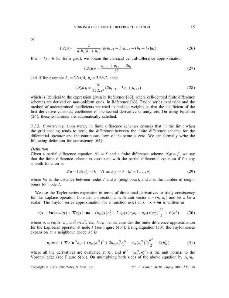
or

(Lhu)I =2

h1h2(h1 + h2)(h2uI−1 + h1uI+1 − (h1 + h2)uI) (26)

If h1 = h2 = h (uniform grid), we obtain the classical central-di�erence approximation:

(Lhu)I =uI−1 + uI+1 − 2uI

h2(27)

and if for example h1 = 3x=4, h2 = 3x=2, then

(Lhu)I =16

27x2(2uI−1 − 3uI + uI+1) (28)

which is identical to the expression given in Reference [63], where cell-centred �nite di�erenceschemes are derived on non-uniform grids. In Reference [63], Taylor series expansion and themethod of undetermined coe�cients are used to �nd the weights so that the coe�cient of the�rst derivative vanishes, coe�cient of the second derivative is unity, etc. On using Equation(26), these conditions are automatically satis�ed.

3.1.3. Consistency. Consistency in �nite di�erence schemes ensures that in the limit whenthe grid spacing tends to zero, the di�erence between the �nite di�erence scheme for thedi�erential operator and the continuous form of the same is zero. We can formally write thefollowing de�nition for consistency [64]:

De�nitionGiven a partial di�erence equation Lv=f and a �nite di�erence scheme Lhv=f, we saythat the �nite di�erence scheme is consistent with the partial di�erential equation if for anysmooth function u,

Lu− (Lhu)I → 0 ∀I as hIJ → 0 (J =1; : : : ; n) (29)

where hIJ is the distance between nodes I and J (neighbour), and n is the number of neigh-bours for node I .

We use the Taylor series expansion in terms of directional derivatives to study consistencyfor the Laplace operator. Consider a direction n with unit vector n=(nx; ny) and let h be ascalar. The Taylor series approximation for a function u(x) at x̃=x+ hn is written as

u(x+ hn)= u(x) +∇u(x) · nh+ (uxx(x)n2x + 2uxy(x)nxny + uyy(x)n2y )h2

2+ O(h3) (30)

where ux ≡ @u=@x, uxx ≡ @2u=@x2, etc. Now, let us consider the �nite di�erence approximationfor the Laplacian operator at node I (see Figure 5(b)). Using Equation (30), the Taylor seriesexpansion at a neighbour (node J ) is

uJ = uI +∇u · nIJ hIJ + (uxx(nIJx )2 + 2uxynIJx nIJy + uyy(nIJy )2)h2

2+ O(h3IJ ) (31)

where all the derivatives are evaluated at xI , and nIJ =(nIJx ; nIJy ) is the unit normal to theVoronoi edge (see Figure 5(b)). On multiplying both sides of the above equation by sIJ =hIJ


16 N. SUKUMAR

(sIJ is the length of the Voronoi edge) and summing over all the neighbours (J =1→ n), weobtain

n∑J=1

sIJhIJuJ =

n∑J=1

sIJhIJuI +∇u ·

n∑J=1

sIJhIJnIJ hIJ

+n∑J=1

sIJhIJ(uxx(nIJx )

2 + 2uxynIJx nIJy + uyy(n

IJy )

2)h2IJ2+ O(h3mIJ ) (32)

where hmIJ = maxJhIJ . Since

∑J sIJ hIJ =O(h2mIJ ) from Equation (19b), the last term which is

of the form∑

J sIJ h2IJ is O(h3mIJ ) after the summation is carried out. The second term on the

right-hand side can be simpli�ed as follows:

∇u ·n∑J=1sIJnIJ =∇u ·

n∑J=1sIJxJ − xIhIJ

(33)

and hence on using Equation (10), we have

∇u ·n∑J=1sIJnIJ =0 (34)

On using the above result and the de�nitions for �IJ and �I that appear in Equation (22),Equation (32) simpli�es to

n∑J=1�IJ uJ − �IuI =

n∑J=1�IJ (uxx(nIJx )

2 + 2uxynIJx nIJy + uyy(n

IJy )

2)h2IJ2+ O(h3mIJ ) (35)

Writing out the normal components (for e.g., nIJx =(xJ − xI)=h), we haven∑J=1�IJ uJ − �IuI =

n∑J=1

�IJ2(uxx(xJ − xI)2 + 2uxy(xJ − xI)(yJ − yI) + uyy(yJ − yI)2) + O(h3mIJ )

(36)

Let

aI =n∑J=1

�IJ2(xJ − xI)2; bI =

n∑J=1

�IJ2(yJ − yI)2; �I =

n∑J=1�IJ (xJ − xI)(yJ − yI) (37)

Then, Equation (36) can be written asn∑J=1�IJ uJ − �IuI = uxxaI + uyybI + uxy�I + O(h3mIJ ) (38)

Using aI and bI , we can write the following identities:

aI =aI + bI2

+aI − bI2

; bI =aI + bI2

− aI − bI2

(39)

or

aI =n∑J=1

�IJ h2IJ4

+ �I =AI + �I ; bI =n∑J=1

�IJ h2IJ4

− �I =AI − �I (40a)



where AI is the area of the Voronoi cell of node I and �I is given by

�I =n∑J=1

�IJ4((xJ − xI)2 − (yJ − yI)2) (40b)

Using the above relations, Equation (38) becomes

n∑J=1�IJ uJ − �IuI = uxx(AI + �I) + uyy(AI − �I) + uxy�I + O(h3mIJ ) (41)

orn∑J=1�IJ uJ − �IuI =∇2uAI + (uxx − uyy)�I + uxy�I + O(h3mIJ ) (42)

We now develop estimates for �I and �I . For each I–J pair, we can write the followingrelations:

xJ − xI = hIJ cos �IJ ; yJ − yI = hIJ sin �IJ (43)

and hence �I in Equation (40b) and �I in Equation (37) can be expressed as

�I =14

n∑J=1�IJ h2IJ (cos

2 �IJ − sin2 �IJ )= 14n∑J=1�IJ h2IJ cos 2�IJ¡

n∑J=1

�IJ h2IJ4

(44a)

�I =n∑J=1�IJ h2IJ cos �IJ sin �IJ =

12

n∑J=1�IJ h2IJ sin 2�IJ¡2

n∑J=1

�IJ h2IJ4

(44b)

and therefore

�I¡AI ⇒ �I =O(h2mIJ ); �I¡2AI ⇒ �I =O(h2mIJ ) (45)

are the best estimates that can be inferred from the above inequality; sharper estimates suchas O(h2+�mIJ ) (�¿0) cannot be established.From Equation (20), we can write the �nite di�erence approximation for the Laplacian as

Lhu=1AI


](46)

and on using Equation (45) and the above equation, we can re-write Equation (42) as

Lhu=∇2u+ O(1) + O(hmIJ ) (47)

since AI =O(h2mIJ ), and therefore in the limit that the grid spacing tends to zero, we have

limhmIJ→0

Lu−Lhu=−O(1) (48)

and hence only zeroth-order consistency is obtained. Truncation error norm computations forthe Poisson problems considered in Section 4.1.2 are in agreement with the above estimate.The above result, however, is not surprising since as opposed to uniform grids in one and

two dimensions, the satisfaction of consistency on irregular grids is in general di�cult. How-ever, the lack of consistency on non-uniform grids as inferred from a Taylor series expansiondoes not preclude convergence [65–68]. This clearly shows that the treatment of consistency


18 N. SUKUMAR

and convergence for �nite di�erence schemes on irregular grids is distinctly di�erent fromthat on uniform grids where consistency (via a Taylor series expansion) and stability arenecessary and su�cient conditions for convergence (Lax–Richtmyer theorem) [64].Kreiss et al. [66] coined the term supraconvergence for schemes that converge at a higher

order than the local truncation error; supraconvergence has received a lot of attention inthe numerical analysis literature for vertex-and cell-centred �nite di�erence schemes. Lazarovet al. [69] provided a theoretical framework to analyse �nite volume cell-centred schemes onuniform Cartesian product grids, whereas in Reference [68], the convergence of block-centredschemes on non-uniform grids is studied. Jones and Menzies [10] showed that cell-centredCartesian product non-uniform grids are inconsistent via a Taylor series expansion, and ex-tended S�uli’s analysis [7] to show that the scheme was however convergent. As opposed to�nite di�erence schemes on regular grids, in �nite volume (di�erence) schemes with irregu-lar nodal spacing, the notion of �ux consistency appears to be the key ingredient to proveconvergence.The �nite di�erence scheme in this paper is derived from a local conservation law, satis�es

the discrete maximum principle as shown in Section 3.1.5, and passes the patch test for theLaplace operator (Section 4.1.1). Using the �nite volume formulation as a starting point,Mishev [8] derived error estimates for a cell-centred di�erence scheme on Voronoi meshes.Clearly, in the present instance, since the �nite di�erence scheme can also be seen in light ofa �nite volume (conservation) method [8], the traditional Taylor series expansion techniqueis not adequate to address consistency, and the convergence analysis conducted in References[8, 10] is to be followed. Remarks on the importance of consistency of the numerical �ux andthe use of a conservation form are also apropos in the development of error estimates for thenumerical solution of scalar conservation laws on irregular Cartesian product grids [70]. Inthis study, we do observe the supraconvergence behaviour with second-order convergence inthe L2 norm for Poisson problems (Section 4.1.2 and 4.1.3).We now show that if the grid is regular (rectangular or hexagonal), the �nite di�erence

scheme is consistent. To this end, using Gauss’s theorem, we can write the following identi-ties: ∫

AI

@(x − xI)@x

d�=∫@AI(x − xI)nx d�=AI (49a)

∫AI

@(y − yI)@y

d�=∫@AI(y − yI)ny d�=AI (49b)

∫AI

@(x − xI)@y

d�=∫@AI(x − xI)ny d�=0 (49c)

Consider Equation (49a) and discretize it on the boundary of the Voronoi cell. Then, we canwrite [42]

n∑J=1(xcIJ − xI)

xJ − xIhIJ

sIJ =AI ; xcIJ =

∫sIJx ds

sIJ(50)

where xcIJ is the x-co-ordinate of the centroid of mass of the Voronoi edge sIJ . In general, thelocation of the centre of mass of the Voronoi facet is not known a priori. If the Delaunay



2

h2

3

1

4

I

h1

Figure 7. Finite di�erence approximation for the Laplacian on a rectangular grid with nodalspacings h1 and h2 in the co-ordinate directions. The Voronoi cell of node I is indicated

by the four dark lines that form a rectangle of area h1h2.

h21η =

0

η

00

0η

ηh

I

η

23h2η =

h

η η

ηη

-6η

-4η

h

Iηη

(a) (b)

Figure 8. Finite di�erence weights for the Laplacian on regular grids. Filled circles are thenatural neighbours of the interior node and the weights for each neighbour are indicated:

(a) square grid; and (b) hexagonal grid.

edge (xI ;xJ ) bisects the Voronoi facet, then xcIJ =(xI + xJ )=2. This is rigorously true forregular grids (see Figures 7 and 8), and hence the above equation reduces to

n∑J=1

�IJ2(xJ − xI)2 =AI (51)

and proceeding likewise with Equations (49b) and (49c), we obtain

n∑J=1

�IJ2(yJ − yI)2 =AI ;

n∑J=1

�IJ2(xJ − xI)(yJ − yI)=0 (52)


20 N. SUKUMAR

Using the above results in Equation (36), with the observation that the coe�cient of the h3mIJterm also vanishes (neighbour pairs with unit normals ± n exist) on a regular grid, we obtain

n∑J=1�IJ uJ − �IuI = uxxAI + uyyAI + O(h4mIJ ) (53)

which reduces to

Lhu=Lu+ O(h2mIJ ) (54)

since AI =O(h2mIJ ), and therefore

limhmIJ→0

Lu−Lhu=0 (55)

and hence the �nite di�erence scheme is consistent on a regular grid.

RemarkIn one dimension, on using the Taylor series expansion, second-order and �rst-order consis-tency are established for regular and irregular nodal discretizations, respectively [38].

3.1.4. Positive-de�niteness. The invertibility (positive-de�niteness) of the discrete matrix Kis studied. To this end, it su�ces if we can show that [63]

(−Lhv; v)¿ 0 ∀v �=0 (v=0 on @�) (56a)

(v; w) =M∑I=1AIvh(xI)wh(xI) (56b)

where M is the number of nodes in the grid, v and w are functions de�ned on the grid(v(xI)= vI ; w(xI)=wI), AI is the area of the Voronoi cell of node I , and the discrete L2

inner product de�ned in Equation (56b) induces the discrete L2 norm given in Equation (78).Using Equation (20), we can write (see Reference [8] too):

(−Lhv; w)=−M∑I=1

M∑J=1J �=I�IJ (vJ − vI)wI (57)

where the second summation has zero contribution for all J which are not neighbours ofnode I (sIJ =0⇒ �IJ =0). By inter-changing I and J in the above equation and noting that�IJ =�JI , we can also write the following equality:

(−Lhv; w)=−M∑J=1

M∑I=1I �=J�JI (vI − vJ )wJ =

M∑I=1

M∑J=1J �=I�IJ (vJ − vI)wJ (58)

On taking the average of Equations (57) and (58) and substituting w= v, we have

(−Lhv; v)=12

M∑I=1

M∑J=1J �=I�IJ (vJ − vI)2 (59)

which is positive if v �=0 and equal to zero if and only if v≡ 0, and hence the positive-de�niteness of the discrete di�usion operator is proven.



We can also sketch an alternate proof of the above using elements from linear algebra. Thesymmetry of K is evident from Equation (21). Let KIJ denote the IJ th entry in the sti�ness

matrix and I =M∑J

J== I

|KIJ |. Then, we have [71]:

PropositionIf K is an irreducible diagonally dominant matrix for which |KJJ |¿J for at least one J; thenK is invertible. The matrix K is said to be diagonally dominant if |KJJ |¿J (J =1; 2; : : : ; M).The matrix K for the di�usion operator in Equation (21) is irreducible (as are most matrices

obtained from �nite di�erence equations [71]). In addition, from Equation (21), we have

|KII |=�I ; I =n∑

K=1�IK =�I (60)

where n is the number of natural neighbours of node I . From the above, we note that thediagonal entry in any row is equal to the sum of the magnitude of the o�-diagonal entrieson the same row. Hence, K is diagonally dominant. Now, if there is at least one essentialboundary condition (say row J ) then |KJJ |¿J for the J th row, and hence the matrix isinvertible. This establishes the positive-de�niteness of K (M -matrix) and the solvability ofthe discrete system.

3.1.5. Discrete maximum principle. The continuous problem (di�usion equation) satis�es themaximum principle and hence for stability any discrete approximation for the di�usion operatormust also obey the maximum principle.

TheoremIf Lhu¿0 on a region, then the maximum value of u on this region is attained on theboundary. Similarly, if Lhu60; then the minimum value of u is attained on the boundary[64].

ProofConsider the region AI (Voronoi cell of node I). Then, on using Equation (20), we can write

(Lhu)I¿0⇒ 1AI


]¿0 (61)

and since AI¿0, we haven∑J=1�IJ uJ − �IuI¿0 (62)

or

�IuI6n∑J=1�IJ uJ (63)

and since �I¿0 (�¿0), we can write

uI6n∑J=1IJ uJ ; IJ =

�IJ�I

(64)


22 N. SUKUMAR

In the above equation, �I =∑

J �IJ , the IJ form a partition of unity and 0¡IJ¡1 ∀J . Theright-hand side of Equation (64) is a convex or barycentric (weights sum to unity) combination(for an n-gon) of its neighbours. The barycentric sum is always bounded between the minimumand maximum of its coe�cients, and since node I is in the interior of the polygon, it followsthat

minJuJ6

n∑J=1IJ uJ6max

JuJ (65a)

uI6n∑J=1IJ uJ (65b)

and hence an interior node can be a (local) maximum only if all its neighbours have thesame maximum value. This completes the proof for the case Lhu¿0. If Lhu60, we have

minJuJ6

n∑J=1IJ uJ6max

JuJ (66a)

n∑J=1IJ uJ6uI (66b)

and we now reach the conclusion that an interior node can be a (local) minimum only if allits neighbours have the same minimum value. This completes the proof for both cases.

RemarkIf L is the Laplacian (�≡ 1), then IJ ≡�IJ , where �IJ is the Laplace shape function fornode J evaluated at xI .

3.1.6. Regular grids. Rectangular and hexagonal grids are used in �nite di�erence methods.In lattice models, Monte Carlo simulations are typically carried out on square and triangularlattices (hexagonal grid) in which periodic boundary conditions are assumed.

Claim 1The Voronoi cell �nite di�erence approximation for the Laplacian reduces to the classical�nite di�erence method for rectangular and hexagonal grids.

ProofThe �rst part is shown for a rectangular grid with nodal spacings h1 and h2 in the co-ordinatedirections (Figure 7). Using Equation (20) and noting that �IJ = �IJ (�≡ 1), we can write the�nite di�erence approximation for the Laplacian (Lh=∇2

h) at node I as

∇2h u=

1AI


]; �IJ =

sIJhIJ; �I =

4∑J=1�IJ (67)

From Figure 7, we note that AI = h1h2, sIJ = h2; hIJ = h1 (J =1; 2), sIJ = h1; hIJ = h2 (J =3; 4),and hence sIJ =hIJ = h2=h1 (J =1; 2) and sIJ =hIJ = h1=h2 (J =3; 4). The above equation reducesto

∇2h u=

1h1h2

[h2h1(u1 + u2) +

h1h2(u3 + u4)− 2

(h1h2+h2h1

)uI

](68)



which simpli�es to

∇2h u=

u1 + u2 − 2uIh21

+u3 + u4 − 2uI

h22(69)

which is the �ve-point �nite di�erence approximation for the Laplacian on a rectangular grid.If h1 = h2 = h, then

∇2h u=

u1 + u2 + u3 + u4 − 4uIh2

(70)

which is the well-known �ve-point stencil for the Laplacian on a square grid. The �nitedi�erence weights for a square grid are shown in Figure 8(a).Consider the hexagonal grid shown in Figure 8(b). Referring to Equation (67), we can

once again write the �nite di�erence approximation for the Laplacian at node I as

∇2h u=

1AI


]; �IJ =

sIJhIJ; �I =

6∑J=1�IJ (71)

For a hexagonal grid, hIJ = h, sIJ = s, and hence �IJ = s=h ∀J . In addition, using Equation(19b), we have AI =6sh=4. Hence, the above equation can be written as

∇2h u=

23sh

[6∑J=1

shuJ − 6s

huI

](72)

and therefore

∇2h u=

23h2

(u1 + u2 + u3 + u4 + u5 + u6 − 6uI) (73)

which is the seven-point stencil (hexagonal grid) for the �nite di�erence method. The �nitedi�erence weights for this case are shown in Figure 8(b). This completes the proof.

3.1.7. Patch test. The proposed �nite di�erence scheme exactly satis�es the Laplace equationwith linear Dirichlet boundary conditions (patch test).

Claim 2The Voronoi cell �nite di�erence approximation passes the patch test for any nodal discretiza-tion.

ProofConsider a domain � that is discretized by M nodes. Let I be an interior node with nneighbours. Then, using Equation (20), the equation for the I th node can be written as(∇2

h u=0):

1AI


]=0 (74)

or

uI =n∑J=1�IJ uJ ; �IJ =

�IJ�I; �IJ =

sIJhIJ; �I =

n∑J=1�IJ (75)


24 N. SUKUMAR

If I is the only interior node (all J are on the boundary), and uJ = a0 + a1xJ + a2yJ is theDirichlet boundary condition (linear �eld), then

uI =n∑J=1�IJ (a0 + a1xJ + a2yJ )= a0 + a1xI + a2yI (76)

since the �IJ form a partition of unity and they also satisfy the linear reproducing conditionsgiven in Equation (11). Hence the solution at an interior node is identical to the exact solution.By a similar extension, if there are more nodes in the interior of the domain, all equationsfor uI that arise are similar to Equation (75) and can hence reproduce the linear �eld exactly.A consequence of the above is that the solution uI at all interior nodes I is identical to theexact solution (linear �eld) evaluated at xI , which completes the proof.

4. NUMERICAL EXAMPLES

Numerical examples for the �nite di�erence scheme on Voronoi grids are presented to demon-strate the accuracy and convergence of the scheme.

4.1. Finite-di�erence scheme on arbitrary grids

Numerical examples are presented for the 2D Poisson equation with Dirichlet boundary con-ditions. The model problem is:

−∇2u(x) =f(x) in � (77a)

u(x) = g(x) on @� (77b)

First we show that the �nite di�erence scheme passes the patch test on uniform as well asnon-uniform grids. Then, convergence studies in the L2 norm are carried out for three testcases to demonstrate the accuracy and convergence of the method. Lastly, numerical resultsfor the Laplace equation in an annulus are presented to demonstrate the performance of thescheme on non-rectangular domains. In our analysis, the L2 and L∞ (maximum) discretenorms are de�ned as

‖u− uh‖2;� =√AI

M∑I=1(u(xI)− uh(xI))2; ‖u− uh‖∞;� = max

I=1;:::;M|u(xI)− uh(xI)| (78)

where u and uh are the exact and the �nite di�erence solutions, respectively, and AI is the areaof the Voronoi cell of node I . The discrete L2 norm in Equation (78) is de�ned analogousto its continuous counterpart—‖u‖L2(�) = (

∫� u

2 d�)1=2.

4.1.1. Patch test. The patch test for the Laplacian operator is carried out: ∇2u=0 in �=(0; 1)× (0; 1), with u= g(x)= x+y (linear �eld) imposed on the boundary of the unit square.The exact solution for this problem is: u(x)= x+y. If the numerical scheme passes the patchtest, then the solution uI at interior nodes must be in agreement (within machine precision)with the exact solution.



(a) (b)

(c)

Figure 9. Patch test: (a) uniform grid (25 nodes); (b) irregular grid (8 nodes);and (c) Random set (70 nodes).

Table I. Errors in the L2 and L∞ norms for the patchtest.

Grids‖u− uh‖2;�

‖u‖2;� ‖u− uh‖∞;�

a 4:9× 10−17 2:2× 10−16

b 3:8× 10−17 1:1× 10−16

c 2:0× 10−16 7:5× 10−16

Three di�erent nodal discretizations [29] are considered (Figure 9), and the relative error inthe L2 norm and the maximum norm are presented in Table I. The results in Table I indicatethat the patch test is passed for regular as well as irregular grids, and hence the numericaltests do con�rm the proof outlined in Section 3.1.7.

4.1.2. Poisson equation in a unit square. Convergence in the L2 norm is studied for theproposed �nite-di�erence scheme. To this end, three Poisson problems are solved in a unitsquare (�= (0; 1) × (0; 1)). The boundary conditions, forcing function, and exact solutionfor the selected examples are given in Table II. In order to conduct the convergence study,


26 N. SUKUMAR

Table II. Numerical tests for the Poisson problem in a unit square.

Problem f(x) g(x) u(x)

I 2x(1− x) + 2y(1− y) 0 x(1− x)y(1− y)

II 22 sin x sin y 0 sin x sin y

III 0 sin x sinh ony=1; sin x sinh y0 otherwise

a Delaunay triangulation mesh generator is used so that uniform grids for a user-speci�eddesired value of h (grid spacing) are obtained. The mesh generator is based on the algorithmdeveloped in Reference [72], in which the initial boundary conforming triangulation is carriedout using the Tanemura-Ogawa-Ogita algorithm [73] and subsequent re�nement is based onincremental point insertion using the Bowyer-Watson algorithm [47, 48]. Re�nement is basedon comparing an actual local length scale ‘ (e.g. element width, circum-radius) to the desiredlength scale speci�ed by a scalar variable which is known as the length density function [72]. In the present instance, since a uniform spacing h is desired in the domain, we set = h(a constant) on all the four sides of the unit square.For the convergence analysis, four grids are considered: h=0:1; 0:05; 0:025; 0:0125. The

nodal grids are shown in Figure 10. The spacing is nearly uniform in the entire domain withthe number of nodes increasing by about a factor of four at every re�nement step. The resultsof the convergence analysis are presented in Figure 11. The error in the discrete L2 norm variesas h�, where � is the rate of convergence. It is seen from Figure 11 that the error decreasesuniformly with decreasing h and the �nite di�erence method has a rate of convergence oftwo in the L2 norm. In Figure 12, the numerical solution (uh) and the error (u− uh) on theunit square (1929 nodal grid) are shown for test problem III. It is observed that the errorsare the most pronounced near y=1. The maximum (absolute) error is 2:6× 10−3, where theexact solution is of the order of 10 (relative error is 0.03%).

4.1.3. Poisson equation in an annulus. To demonstrate the accuracy of the proposed techniqueon non-rectangular domains, we solve the Poisson equation in an annulus which is boundedbetween two concentric cylinders of radius r=1 and 2:

−∇2u(r; �) =f(r; �) in 1¡r¡2 (79a)

u(1; �) = �u1(�); u(2; �)= �u2(�) (79b)

which in electrostatics is the model problem for the potential in the presence of a chargedistribution in the domain—u is the potential, f is the charge density, and E=−∇u (�ux)is the electric �eld (force per unit charge).Numerical tests are presented for three problems:

I. The Laplace equation (no charges) with the potential a constant on both the inner andthe outer boundaries ( �u1 = 0, �u2 = 1) is considered. Owing to symmetry, the Laplace



(a) (b)

(d)(c)

Figure 10. Nodal grids for the Poisson problems in a unit square: (a) 138 nodes;(b) 509 nodes; (c) 1929 nodes; and (d) 7542 nodes.

-5 -4 -3 -2loge h

-12

-10

-8

-6

-4

log e

(R

elat

ive

erro

r in

L2 n

orm

) Test I (λ = 2.0)Test II (λ = 2.0)Test III (λ = 2.1)

Figure 11. Rate of convergence for Poisson problems in a unit square.The convergence rate � is indicated.

equation reduces to the 1D radial equation: urr + ur=r=0 with the exact solution:

u(r)=ln(r)ln(2)

(80)

II. As a second test, we consider the Laplace equation with boundary conditions that varywith �: �u1 = 1+cos �, and �u2 = 2+cos �. The exact solution using separation of variables


28 N. SUKUMAR

X

Y

Z

uh10.826910.1051

9.38348.66167.93987.21806.49625.77445.05264.33083.60902.88722.16541.44360.7218

X

Y

0 0.3 0.4 0.5 0.6 0.7 0.8 0.90.20.1 10

0.1

0.2

0.3

0.4

0.5

0.6

0.7

0.8

0.9

1

u - uh0.00220.00190.00160.00120.00090.00060.0003

-0.0001-0.0004-0.0007-0.0010-0.0014-0.0017-0.0020-0.0023

(a) (b)

Figure 12. Numerical solution and error for test problem III: (a) uh; and (b) u− uh.

can be written as

u(r; �)=1 +ln(r)ln(2)

+[r3+23r

]cos � (81)

III. Lastly, the Poisson problem with a charge distribution f(r; �)=−(15r2 − 24r + 6) sin �and with homogeneous boundary conditions �u1 = �u2 = 0 is studied. The exact solution isgiven by [74]

u(r; �)= (r4 − 3r2 + 2r2) sin � (82)

Four nodal grids are used to carry out a convergence study. In generating the nodal grids,a constant value of = h is speci�ed on both the inner radius (r=1) as well as the outerradius (r=2). The nodal grids used in the analysis are shown in Figure 13 with the averagegrid spacing h==8; =16; =32, and =64. The relative error in the L2 norm is plotted inFigure 14, and it is seen that even for a non-rectangular domain, the second-order accuracyof the method is preserved. In Figure 15, the numerical solution for the �nest grid is plotted.The symmetry in the potential structure is captured, and the maximum error in the domain(point-wise estimate at the nodes) is 0.4%.

5. CONCLUSIONS

In this study, we have presented some of our recent �ndings on the Laplace interpolant andhave provided a basis for its use as a suitable weight measure for unstructured grids. TheVoronoi diagram and the notion of natural neighbours were used as the building blocks indescribing the link between discrete nodes on an irregular grid. A detailed account of the



(a) (b)

(d)(c)

Figure 13. Nodal grids for the Poisson problems in an annulus: (a) 96 nodes;(b) 346 nodes; (c) 1257 nodes; and (d) 4744 nodes.

previous developments of the Laplace interpolant was presented, and then the Laplace weightwas used to construct a robust and accurate Voronoi cell �nite di�erence method for arbitraryunstructured grids.The Voronoi cell �nite di�erence scheme that was proposed was distinctive in many re-

spects; some of the key advantages of the numerical method were as follows:

1. Liszka and Orkisz [3] recognized the importance of spatial nodal arrangements and appro-priate geometries of the computational cell that rendered well-conditioned and solvablesystem of equations. Natural neighbours present a very appealing construct in de�ningneighbour relations on an arbitrary grid, and hence it is evident that using this notionin the construction of a discrete approximation is of merit. In addition, as opposed toearlier approaches which rely on Euclidean distances to de�ne the computational cell fora node, here the use of the Voronoi polygon was a natural choice.


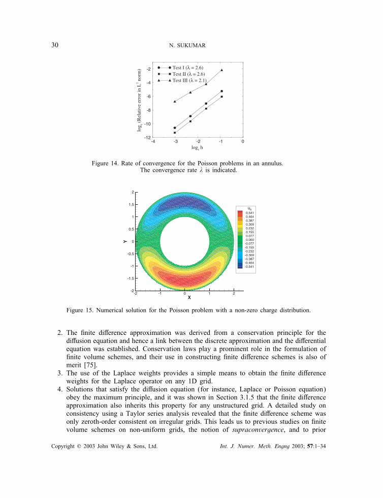
30 N. SUKUMAR

-4 -3 -2 -1 0loge h

-12

-10

-8

-6

-4

-2

log e (

Rel

ativ

e er

ror

in L

2 nor

m) Test I (λ = 2.6)

Test II (λ = 2.6)Test III (λ = 2.1)

Figure 14. Rate of convergence for the Poisson problems in an annulus.The convergence rate � is indicated.

X

Y

-2 -1 0 1 2-2

-1.5

-1

-0.5

0

0.5

1

1.5

2

uh0.5410.4640.3870.3090.2320.1550.0770.000

-0.077-0.155-0.232-0.309-0.387-0.464-0.541

Figure 15. Numerical solution for the Poisson problem with a non-zero charge distribution.

2. The �nite di�erence approximation was derived from a conservation principle for thedi�usion equation and hence a link between the discrete approximation and the di�erentialequation was established. Conservation laws play a prominent role in the formulation of�nite volume schemes, and their use in constructing �nite di�erence schemes is also ofmerit [75].

3. The use of the Laplace weights provides a simple means to obtain the �nite di�erenceweights for the Laplace operator on any 1D grid.

4. Solutions that satisfy the di�usion equation (for instance, Laplace or Poisson equation)obey the maximum principle, and it was shown in Section 3.1.5 that the �nite di�erenceapproximation also inherits this property for any unstructured grid. A detailed study onconsistency using a Taylor series analysis revealed that the �nite di�erence scheme wasonly zeroth-order consistent on irregular grids. This leads us to previous studies on �nitevolume schemes on non-uniform grids, the notion of supraconvergence, and to prior



theoretical work [8, 10] to provide support for the convergence of the method. The useof a balance law (�ux conservation) to construct the di�erence scheme, in tandem withthe satisfaction of the patch test and the added stability lead to second-order convergence(supraconvergence) for the problems considered in this study.

5. The di�usion operator is self-adjoint, and the discrete di�usion operator results in asymmetric positive-de�nite sti�ness matrix. This was a consequence of the symmetryof the Laplace weight (�IJ=�JI). Most �nite di�erence and �nite volume schemes forthe di�usion (Laplace) operator on irregular grids yield a non-symmetric matrix. If theSibson shape function or those based on MLS schemes are used as weights in a �nitedi�erence scheme, in general a non-symmetric sti�ness matrix would result.

6. Only simple geometric computations are required to evaluate the �nite di�erence weight-ing functions, and hence the computational costs involved in the �nite di�erence schemeare minimal. In 3D, the only additional complexity that arises is in the computation ofsIJ which is a polygonal area (Voronoi facet) [38].

The numerical simulations in this paper have demonstrated the promise of the Laplace weightas an appropriate measure on unstructured grids. The use of a local conservation principleto derive the �nite di�erence (or equivalently collocation) scheme is of relevance in nodalintegration techniques within meshless methods [60], and also in hydrodynamic simulationsusing particle methods where local conservation is desirable [76]. On considering integralidentities and rules of vector algebra on lattices networks, a general framework can possiblyemerge for the construction of �nite di�erence approximations on unstructured grids thatinvolve the gradient and divergence of vectors as well as higher-order tensors.

ACKNOWLEDGEMENTS

It is a pleasure to acknowledge John Bolander and Tim Ginn for many stimulating discussions, and fortheir comments on an earlier draft of this paper; the author is also grateful to Tim Ginn for pointingout the related work in Reference [58]. Parts of this study were completed during the spring of 2001,when the author was at the Princeton Materials Institute; the hospitality extended to him by DavidSrolovitz at Princeton University is appreciated. Tim Baker is also thanked for providing the Delaunaytriangulation code, which was used to generate the grids considered in the convergence study.

REFERENCES

1. Belytschko, T, Krongauz, Y, Organ, D, Fleming, M, Krysl P. Meshless methods: an overview and recentdevelopments. Computer Methods in Applied Mechanics and Engineering 1996; 139:3–47.

2. Jensen PS. Finite di�erence techniques for variable grids. Computers and Structures 1972; 2:17–29.3. Liszka T, Orkisz J. The �nite di�erence method at arbitrary irregular grids and its application in appliedmechanics. Computers and Structures 1980; 11:83–95.

4. Breitkopf P, Touzot G, Villon P. Double grid di�use collocation method. Computational Mechanics 2000;25(2=3):199–206.

5. Lancaster P, Salkauskas K. Surfaces generated by moving least squares methods. Mathematics of Computation1981; 37:141–158.

6. Baty RS, Villon WP. Least-squares solutions of a general numerical method for arbitrary irregular grids.International Journal for Numerical Methods in Engineering 1997; 140:1701–1717.

7. S�uli E. Convergence of �nite volume schemes for Poisson’s equations on nonuniform meshes. SIAM Journalon Numerical Analysis 1991; 28(5):1419–1430.

8. Mishev ID. Finite volume methods on Voronoi meshes. Numerical Methods for Partial Di�erential Equations1998; 14:193–212.

9. Hermeline F. A �nite volume method for the approximation of di�usion operators on distorted meshes. Journalof Computational Physics 2000; 160:481–499.


32 N. SUKUMAR

10. Jones WP, Menzies KR. Analysis of the cell-centred �nite volume method for the di�usion equation. Journalof Computational Physics 2000; 165:45–68.

11. Petrovskaya NB. Modi�cation of a �nite volume scheme for Laplace’s equation. SIAM Journal on Scienti�cComputing 2001; 23(3):891–909.

12. Christie I, Hall C. The maximum principle for bilinear elements. International Journal for Numerical Methodsin Engineering 1984; 20:549–553.

13. Putti M, Cordes C. Finite element approximation of the di�usion operator on tetrahedra. SIAM Journal onScienti�c Computing 1998; 19(4):1154–1168.

14. Li S, Liu WK. Meshfree and particle methods and their applications. Applied Mechanics Reviews 2002; 55(1):1–34.

15. Melenk JM, Babu�ska I. The partition of unity �nite element method: Basic theory and applications. ComputerMethods in Applied Mechanics and Engineering 1996; 139:289–314.

16. Duarte CA, Oden JT. An H -p adaptive method using clouds. Computer Methods in Applied Mechanics andEngineering 1996; 139:237–262.

17. Sibson R. A vector identity for the Dirichlet tessellation. Mathematical Proceedings of the CambridgePhilosophical Society 1980; 87:151–155.

18. Sibson R. A brief description of natural neighbor interpolation. In Interpreting Multivariate Data, Barnett V(ed.). John Wiley: Chichester, 1981; 21–36.

19. Okabe A, Boots B, Sugihara K. Spatial Tessellations: Concepts and Applications of Voronoi Diagrams. Wiley:Chichester, 1992.

20. Bern M, Eppstein D. Mesh generation and optimal triangulation. In Computing in Euclidean Geometry, DuD-Z, Hwang FK (eds). Lecture Notes Series on Computing, vol. 1. World Scienti�c: Singapore, 1995; 23–90.

21. Belikov VV, Ivanov VD, Kontorovich VK, Korytnik SA, Semenov AYu. The non-Sibsonian interpolation: A newmethod of interpolation of the values of a function on an arbitrary set of points. Computational Mathematicsand Mathematical Physics 1997; 37(1):9–15.

22. Belikov VV, Semenov AYu. New non-Sibsonian interpolation on arbitrary system of points in Euclidean space.In 15th IMACS World Congress, Numerical Mathematics, vol. 2. Wissen Tech. Verlag: Berlin, 1997; 237–242.

23. Belikov VV, Semenov AYu. Non-Sibsonian interpolation on arbitrary system of points in Euclidean space andadaptive isolines generation. Applied Numerical Mathematics 2000; 32(4):371–387.

24. Sugihara K. Surface interpolation based on new local coordinates. Computer-Aided Design 1999; 31:51–58.25. Hiyoshi H, Sugihara K. Two generalizations of an interpolant based on Voronoi diagrams. International Journal

of Shape Modeling 1999; 5(2):219–231.26. Hiyoshi H, Sugihara K. Voronoi-based interpolation with higher continuity. In Proceedings of the 16th Annual

ACM Symposium on Computational Geometry, 2000; 242–250.27. Braun J, Sambridge M. A numerical method for solving partial di�erential equations on highly irregular evolving

grids. Nature 1995; 376:655–660.28. Sukumar N. The natural element method in solid mechanics. Ph.D. Thesis, Theoretical and Applied Mechanics,

Northwestern University, Evanston, IL, U.S.A., June 1998.29. Sukumar N, Moran B, Belytschko T. The natural element method in solid mechanics. International Journal for

Numerical Methods in Engineering 1998; 43(5):839–887.30. Sukumar N, Moran B. C1 natural neighbor interpolant for partial di�erential equations. Numerical Methods for

Partial Di�erential Equations 1999; 15(4):417–447.31. Bueche D, Sukumar N, Moran B. Dispersive properties of the natural element method. Computational Mechanics

2000; 25(2=3):207–219.32. Sukumar N, Moran B, Semenov AYu, Belikov VV. Natural neighbor Galerkin methods. International Journal

for Numerical Methods in Engineering 2001; 50(1):1–27.33. Sukumar N. Sibson and non-Sibsonian interpolants for elliptic partial di�erential equations. In Proceedings of

the First MIT Conference on Fluid and Solid Mechanics, vol. 2, Bathe KJ (ed.). Elsevier Press: Amsterdam,The Netherlands, 2001; 1665–1667.

34. Cueto E, Doblar e M, Gracia L. Imposing essential boundary conditions in the natural element method by meansof density-scaled �-shapes. International Journal for Numerical Methods in Engineering 2000; 49(4):519–546.

35. Garc ia JM, Cueto E, Doblar e M. Simulation of bone internal remodeling by means of the �-shape-based naturalelement method. In European Congress on Computational Methods in Applied Sciences and Engineering,ECCOMAS 2000, Barcelona, Spain, 2000.

36. Moran B, Yoo J. Meshless methods for life cycle engineering simulation: natural neighbor formulations. InModeling and Simulation-Based Life Cycle Engineering Simulation, Chong KP, Saigal S, Thynell S, Morgan H(eds). Taylor and Francis: London, 2001; 91.

37. Cueto E, Calvo B, Doblar e M. Modelling three-dimensional piece-wise homogeneous domains using the�-shape-based natural element method. International Journal for Numerical Methods in Engineering 2002;54(6):871–897.



38. Sukumar N, Bolander Jr. JE. Numerical computation of discrete di�erential operators on non-uniform grids.2002, submitted.

39. Martinez MA, Cueto E, Doblar e M, Chinesta F. Natural element meshless simulation of injection processesinvolving short �ber suspension. Journal of Non-Newtonian Fluid Mechanics, 2003, in press.

40. Christ NH, Friedberg R, Lee TD. Random lattice �eld-theory—general formulation. Nuclear Physics B 1982;202(1):89–125.

41. Christ NH, Friedberg R, Lee TD. Gauge-theory on a random lattice. Nuclear Physics B 1982; 210(3):310–336.42. Christ NH, Friedberg R, Lee TD. Weights of links and plaquettes in a random lattice. Nuclear Physics B 1982;

210(3):337–346.43. Belytschko T, Lu YY, Gu L. Element-free Galerkin methods. International Journal for Numerical Methods in

Engineering 1994; 37:229–256.44. Yavari A, Kaveh A, Sarkani S, Bondarabady HAR. Topological aspects of meshless methods and nodal

ordering for meshless discretizations. International Journal for Numerical Methods in Engineering 2001; 52(9):939–978.

45. Lawson CL. Software for C1 surface interpolation. In Mathematical Software III, vol. 3, Rice JR (ed.).Academic Press: New York, NY, 1977.

46. Gr�unbaum B. Convex Polytopes. Wiley: New York, 1967.47. Bowyer A. Computing Dirichlet tessellations. The Computer Journal 1981; 24:162–166.48. Watson DF. Computing the n-dimensional Delaunay tessellation with application to Voronoi polytopes. The

Computer Journal 1981; 24(2):167–172.49. Beale PD, Srolovitz DJ. Elastic fracture in random materials. Physics Review B 1988; 37(10):5500–5507.50. Jagota A, Bennison SJ. Spring-network and �nite-element models for elasticity and fracture. In Nonlinearity and

Breakdown in Soft Condensed Matter. Springer Lecture Notes in Physics, vol. 437, Bardhan KK, ChakrabartiBK, Hansen A (eds). Springer: Berlin, 1994; 186–201.

51. Jagota A, Bennison SJ. Element breaking rules in computational models for brittle fracture. Modelling andSimulation in Materials Science and Engineering 1995; 3(4):485–501.

52. Bolander Jr JE, Saito S. Fracture analyses using spring networks with random geometry. Engineering FractureMechanics 1998; 61:569–591.

53. Bolander Jr JE, Yoshitake K, Thomure J. Stress analysis using elastically uniform rigid-body spring networks.Journal of Structural Mechanics and Earthquake Engineering 1999; 633=I-49:25–32.

54. Harris SC, Williams D, Sibson R. Scaling random walks on arbitrary sets. Mathematical Proceedings of theCambridge Philosophical Society 1999; 125(3):535–544.

55. Ghosh S, Mukhopadhyay SN. A material based �nite-element analysis of heterogeneous media involvingDirichlet tessellations. Computer Methods in Applied Mechanics and Engineering 1993; 104(2):211–247.

56. Ghosh S, Moorthy S. Elastic–plastic analysis of arbitrary heterogeneous materials with the Voronoi cell �nite-element method. Computer Methods in Applied Mechanics and Engineering 1995; 121(1–4):373–409.

57. Friedberg R, Ruiz M. Vector algebra on a lattice. Physical Review D 1984; 29(12):2916–2918.58. Narasimhan TN, Witherspoon PA. An integrated �nite di�erence method for analyzing �uid �ow in porous

media. Water Resources Research 1976; 12(1):57–64.59. Aluru NR. A point collocation method based on reproducing kernel approximations. International Journal for

Numerical Methods in Engineering 2000; 47:1083–1121.60. Chen JS, Wu CT, Yoon S, You Y. A stabilized conforming nodal integration for Galerkin meshfree methods.

International Journal for Numerical Methods in Engineering 2001; 50:435–466.61. B�orgers C, Peskin CS. A Lagrangian method based on the Voronoi diagram for the incompressible Navier–

Stokes equations on a periodic domain. In The Free Lagrange Method (Lecture Notes in Physics), vol. 238,Frills MJ, Crowley WP, Trease H (eds). Springer-Verlag: New York, 1985; 87–113.

62. B�orgers C, Peskin CS. A Lagrangian fractional step method for the incompressible Navier–Stokes equations ona periodic domain. Journal of Computational Physics 1987; 70:397–438.

63. Thomas JW. Numerical Partial Di�erential Equations: Finite Di�erence Methods. Springer-Verlag: New York,1995.

64. Strikwerda JC. Finite Di�erence Schemes and Partial Di�erential Equations. Chapman & Hall, CRC: BocaRaton, FL, 1999.

65. Tikhonov AN, Samarskii AA. Homogeneous di�erence schemes on non-uniform nets. U.S.S.R ComputationalMathematics and Mathematical Physics 1962; 2:927–953.

66. Kreiss H-O, Manteu�el TA, Swartz B, Wendro� B, White Jr AB. Supra-convergent schemes on irregular grids.Mathematics of Computation 1986; 47(176):537–554.

67. Manteu�el TA, White Jr. AB. The numerical solution of second-order boundary value problems on nonuniformmeshes. Mathematics of Computation 1986; 47(176):511–535.

68. Weiser A, Wheeler MF. On convergence of block-centered �nite di�erences for elliptic problems. SIAM Journalon Numerical Analysis 1998; 25(2):351–375.

69. Lazarov RD, Mishev ID, Vassilevski PS. Finite volume methods for convection-di�usion problems. SIAMJournal on Numerical Analysis 1996; 33(1):31–55.


34 N. SUKUMAR

70. Cockburn B, Gremaud P-A, Yang JX. A priori error estimates for numerical methods for scalar conservation lawspart III: Multidimensional �ux-splitting monotone schemes on non-cartesian grids. SIAM Journal on NumericalAnalysis 1998; 35(5):1775–1803.

71. Thomas JW. Numerical Partial Di�erential Equations: Conservation Laws and Elliptic Equations. Springer-Verlag: New York, 1999.

72. Baker TJ. Triangulations, mesh generation and point placement strategies. In Frontiers of Computational FluidDynamics, Caughey DA, Hafez MM (eds). Wiley: New York, NY, 1994; 101–115.

73. Tanemura M, Ogawa T, Ogita W. A new algorithm for three-dimensional Voronoi tessellation. Journal ofComputational Physics 1983; 51:191–207.

74. Christopher I, Knorr G, Shoueri M, Bertrand P. Solution of the Poisson equation in an annulus. Journal ofComputational Physics 1997; 131:323–326.

75. Shashkov M. Conservative Finite-Di�erence Methods on General Grids. CRC Press: Boca Raton, FL, 1996.76. Dilts GA. Moving least-square particle hydrodynamics II: Conservation and boundaries. International Journal

for Numerical Methods in Engineering 2000; 48:1503–1524.


vornoi fdm

Documents

nite dierence schemes

classical nite dierence

nite volume schemesare

laplace weight

proposed scheme

laplace interpolant

laplace interpolant

wellknown numerical