vortex pinning in high-tc...

Vortex Pinning in High-Tc Superconductors

A thesis submitted in partial fulfillment of the requirementfor the degree of Bachelor of Science

Physics from the College of William and Mary in Virginia,

by

Abigail C. Shockley

Accepted for: BS in Physics

Advisor: W. J. Kossler

Gina Hoatson

Williamsburg, VirginiaMay 2007

Abstract

We have studied vortex pinning in High-Tc superconductors by examining experimental µ-

SR data collected at TRIUMF. Using the theoretical model for vortex pinning proposed by

E.H. Brandt, we have analyzed the second moment of the magnetic field for the superconductor

BSCCO. We used four different theoretical models for the behavior of the penetration depth in

a superconductor to determine whether BSCCO could be considered d-wave or s-wave.

i

Acknowledgements

I would first like to thank my research advisor, Jack Kossler, for not only providing me guidance on

this project but for providing support with my personal issues as well. On that note, I would also

like to thank Marc Sher, Jeff Nelson, Jan Chaloupka, and Gina Hoatson for providing a similar form

of guidance. The physics department has miraculously helped me keep myself together and finish

out this year. I don’t know that I can fully express my gratitude in words.

ii

Contents

1 Introduction 1

1.1 London Equation . . . . . . . . . . . . . . . . . . . . . . . . . . . . . . . . . . . . . . 1

1.2 Penetration Depth . . . . . . . . . . . . . . . . . . . . . . . . . . . . . . . . . . . . . 2

1.3 Coherence Length . . . . . . . . . . . . . . . . . . . . . . . . . . . . . . . . . . . . . 3

1.4 Type II Superconductor . . . . . . . . . . . . . . . . . . . . . . . . . . . . . . . . . . 3

1.5 Empirical Model . . . . . . . . . . . . . . . . . . . . . . . . . . . . . . . . . . . . . . 4

1.6 2-Fluid Model . . . . . . . . . . . . . . . . . . . . . . . . . . . . . . . . . . . . . . . . 4

1.7 BCS Model . . . . . . . . . . . . . . . . . . . . . . . . . . . . . . . . . . . . . . . . . 5

1.8 D-wave Model . . . . . . . . . . . . . . . . . . . . . . . . . . . . . . . . . . . . . . . . 8

1.9 Pinning Model for Vortex Line Behavior . . . . . . . . . . . . . . . . . . . . . . . . . 9

1.10 Second Moment Model . . . . . . . . . . . . . . . . . . . . . . . . . . . . . . . . . . . 12

1.11 Penetration Depth and the Theoretical Models . . . . . . . . . . . . . . . . . . . . . 12

2 Experiment 14

2.1 µ-SR Technique . . . . . . . . . . . . . . . . . . . . . . . . . . . . . . . . . . . . . . . 14

2.2 Heterodyne Technique . . . . . . . . . . . . . . . . . . . . . . . . . . . . . . . . . . . 14

2.3 Fitting the Data . . . . . . . . . . . . . . . . . . . . . . . . . . . . . . . . . . . . . . 18

2.3.1 Function 34 . . . . . . . . . . . . . . . . . . . . . . . . . . . . . . . . . . . . . 18

2.3.2 Function 35 . . . . . . . . . . . . . . . . . . . . . . . . . . . . . . . . . . . . . 19

2.3.3 Which function to use? . . . . . . . . . . . . . . . . . . . . . . . . . . . . . . 19

3 Results 23

4 Conclusion 35

iii

1 Introduction

Historically, Kammerlingh Onnes discovered the first superconductor (mercury) in

1911. Superconductors have the unusual property that under a certain temperature

they have zero electrical resistance [1]. In 1956, Cooper proposed that two electons

interacting with each other in a Fermi sea background form bound states for an

arbitrarily weak attractive force. The resulting bound electron pairs are called Cooper

pairs and become the carriers of the super-current [2]. In general, there are two main

types of superconductors: Type I and Type II. High-Tc superconductors are classified

as Type II.

1.1 London Equation

The London equation allows us to determine the magnetic field distribution of a

superconductor explicitly [1]. This field distribution depends primarily upon the

penetration depth which is one of the characteristic parameters of a superconductor.

We will start by considering one of Maxwell’s equations, which in Gaussian units

is:

∇× B =4π

cj (1)

To find a second relation for the current density j, consider an electron with charge

e moving at velocity v at time 0. The current density can then be expressed as

j = nsev (2)

where ns is the number of superconducting electrons. Taking the time derivative of

Eq 2,

dj

dt= nsea =

nse2

mE (3)

1

where a is the acceleration due to an electric field E and m is the mass of an electron.

From another one of Maxwell’s equations, the electric field is related to the magnetic

field:

∇× E = −1

c

dB

dt(4)

Inserting Eq 4 into Eq 3, integreating and arbitrarily setting the integration con-

stant to zero, we have

∇× j = −nse2

mcB or j = −kA (5)

Returning to Eq 1, we want a relation involving the curl of j.

4π

c∇× j = ∇× (∇× B)

= ∇(∇ ·B) −∇2B

Using Maxwell’s equation ∇·B = 0 and Eq 5, we have

∇2B − 4πne2

mc2B = 0 (6)

which is known equivalently with Eq 5 as the London equation. This equation was

first proposed by F. and H. London [1].

1.2 Penetration Depth

The penetration depth is defined as

λL =

(

mc2

4πnse2

)12

(7)

where ns is the number of superconducting electrons so that Eq 6 reads

∇2B − 1

λ2L

B = 0 (8)

2

In a plane geometry situation, the field in a superconductor falls off as H0e−x/λL .

This justifies the description of λL as a penetration depth.

1.3 Coherence Length

Degennes [1] discusses the coherence length which is roughly the size of the cooper

pair. Our derivation of the London equation assumes a slow variation in space of the

supercurrent j. In order for the London equation to be valid, we must define what is

meant by slow. The velocities of two electrons are correlated if the distance between

them is smaller than a certain range. For pure metals, the correlation length is called

ξ0. Our derivation applies when the supercurrent has a negligible variation over

distances ∼ ξ0. To estimate ξ0 we notice that the important domain in momentum

space is defined by

EF − ∆ <p2

2m< EF + ∆ (9)

where EF is the Fermi level and ∆ is the energy gap. The gap is related to the

transition temperature by 2∆ = 3.5kBT0. Considering a Fermi sphere, the thickness

of the shell is defined by Eq 9 as δp ∼= 2∆vF

. From the uncertainty principle, the

minimum spatial extent is δx ∼ hδp

. We can then take

ξ0 =hvF

π∆(10)

where the factor 1π

is arbitrary. The length ξ0 in Eq 10 is called the coherence length

of a superconductor. [1]

1.4 Type II Superconductor

For transition metals and intermetallic compounds, the effective mass is very large, λL

is large (∼= 2700A) and the Fermi velocity is small (∼= 106cm/sec). For our purposes,

3

we are considering compounds with a relatively high transition temperature (∼= 90K).

The gap ∆ is roughly proportional to the transition temperature and is therefore

larger. For all these reasons, ξ0 is very small (∼= 30A) for high Tc materials. For this

class of materials, Eq 9 is applicable in weak fields. These materials are called Type

II or London superconductors. [1]

1.5 Empirical Model

The simplest form of the temperature dependence of the penetration depth is given

by

(

λ

λ0

)2

=1

1 − ( TTc

)γ(11)

where γ is an exponent. A phenomenological description of the penetration depth

may be achieved with γ = 2.0 [3]. This simple model is often referred to as the

Empirical Model.

1.6 2-Fluid Model

For the developement of the 2-Fluid Model, we will examine the magnetic properties

of a superconducting sample. For a very small sample, we must take the average

value of the magnetic field. Considering a plate of thickness 2a [4],

B =1

a

∫ a

0Hdx = H0

(

1 − 2γa2

3λ2

)

(12)

The magnetic susceptibility κ for a sample is then

κ =B − H0

4πH0= − γa2

6πλ2(13)

where γ is a constant depending on the theory of penetration and the geometry of

the sample. Or

4

κ

κ0

=αa2

λ2(14)

where α is a constant whose value depends on whether we are considering a plate,

a wire or a sphere. Since γ is an unspecified parameter, there is little point in

considering the full calculation of κκ0

.

Considering the normalized susceptibility over an assembly of spheres, we have

κ

κ0=

αa′2

λ2(15)

where a’2 = a5/a3 provided that a ≪ λ for all spheres. Looking at κκ0

as a function

of temperature, we find that the variation can be due only to a variation of λ with

temperature. Since a’ is only known to an order of magnitude, we may only consider

relative values of λ. Experimental data is consistent with the law

(

λ

λ0

)2

=1

1 − ( TTc

)4(16)

which is commonly referred to as the 2-Fluid Model. [4]

1.7 BCS Model

Degennes [1] discusses the derivation of the BCS model. We first define a wave

function such that

φ = cΠk(1 + gka+k↑a

+−k↓)φ0 (17)

where the product extends over all plane wave states, k, c is a normalization constant,

and uk and vk are real. The operator a+kα creates an electron in the state (kα) when

operating on the state described by φ0. By incorporating the factor c into the product,

we obtain

5

φ = Πk(uk + vka+k↑a

+−k↓)φ0 (18)

with

vk

uk

= gk u2k + v2

k = 1 (19)

Letting H be the Hamiltonian of the interacting electron system, we can use the

variational principle to minimize the expression

< φ | H | φ > −EF < φ | N | φ > (20)

where N is the average number of particles and EF , a Lagrange multiplier, is the

Fermi energy.

In order to minimize < φ | H | φ > taking account of the relation u2k + v2

k = 1, we

set

ul = sin θl vl = cos θl (21)

< φ | H | φ >= 2∑

k

ξk cos2 θk +1

4

∑

kl

sin 2θk sin 2θlVkl (22)

where Vkl is a term that represents the interaction energy for the transition of a pair

of electrons from the state (k↑,-k↓) to the state (l↑,-l↓) and ξk = h2k2

2m− EF . The

minimization equations are

0 =∂

∂θk

< φ | H | φ >= −2ξk sin 2θk +∑

l

cos 2θk sin 2θlVkl (23)

or

ξk tan 2θk =1

2

∑

l

Vkl sin 2θl (24)

We define

6

∆k = −∑

l

Vklulvl (25)

ǫl =√

(ξ2l + ∆2

l ) (26)

and we find

tan 2θl = −∆l

ξl

(27)

2ulvl = sin 2θl =−∆l

ξl(28)

−u2k + v2

k = cos 2θk = −ξk

ǫk(29)

Inserting the value of ulvl into Eq 25, we obtain an expression for ∆

∆k = −∑

l

Vkl∆l

2(ξ2l + ∆2

l )12

(30)

The BCS interaction is chosen as

Vkl = −V if | ξk |, | ξl |≤ hωD

= 0 otherwise

where ωD is a frequency. Then we have

∆k = 0 for | ξk |> hωD

∆k = ∆ (independent of k) for | ξk |< hωD

We can now write

7

∆ = N(0)V∫ hωD

−hωD

∆dξ

2(∆2 + ξ2)12

(31)

where N(0) is the number of electrons at the Fermi level. This can be solved for ∆.[1]

At finite temperatures, it can be shown [5] that Eq 31 can be rewritten as

1

N(0)V=∫ hωD

0

tanh 12β(ξ2 + ∆2)

12

(ξ2 + ∆2)12

dξ (32)

which yields a ∆(T ).

In Fourier space, Eq 5 generalizes to

j(q) =−c

4πK(q)A(q) (33)

for an isotropic system.

From this, one can show that

K(0, T ) = λ−2L (T ) = λ−2

L (0)

[

1 − 2∫ ∞

∆

(

− ∂f

∂E

)

E

(E2 − ∆2)12

dE

]

(34)

1.8 D-wave Model

A generalization of the BCS model for the situation in which the interaction energy

has D-wave symmetry has been introduced by Anderson and Morel [6]. Using this

model, Amin et. al. [7] generalized the BCS connection between the vector potentila

and current of Eq 33 to

jk = − c

4πQ(k)Ak (35)

where Q(k) is the electromagnetic response tensor. From Amin [7], one finds that

in solving the Gorkov equations generalized for an anisotropic gap the kernel of Q is

Qij(k) =4πT

λ20

∑

n>0

<∆2

pvFivFj

(ω2n + ∆2

p)12 (ω2

n + ∆2p + γ2

k)> (36)

8

where γk = vF · k2, λ0 is the London penetration depth, ωn = πT (2n − 1) are the

Matsubara frequencies and the angular bracket means Fermi surface averaging. For

the purposes of this paper, we will not go into further detail on the latter two subjects.

We write the London equation solely in terms of magnetic field:

Bk − k × [Q−1

(k)(k × Bk)] = 0 (37)

To account for the phase winding around the vortex cores, we insert a source term

F(k)= e−ξ20k2/2 on the right hand side of Eq 37.

We define λeff by

λ−4eff = λ−4

0 (¯δB2

¯δB20

) (38)

where ¯δB2 is the second moment of the field distribution in the vortex lattice and

¯δB20 is the same quantity for the magnetic field B0(r) obtained by solving the London

model for a triangular lattice with the same B and λ0. Using Eq 37 and 38, we find

λ−4eff = C

∑

k 6=0

e−ξ20k2

(1 + Lijkikj)2≈ C

∑

k 6=0

e−ξ20

(Lijkikj)2(39)

where k are the reciprocal lattice wave vectors and

Lij(k) =Qij(k)

detQ(k), C−1 =

∑

k 6=0

e−ξ20k2

k4. (40)

1.9 Pinning Model for Vortex Line Behavior

In a highly anisotropic superconductor, an individual vortex can be represented as

a stack of two-dimensional vortices which create a Vortex-Line Lattice (VLL). In

the lowest energy configuration in the absence of pinning and thermal vibration, the

vortex-line will be straight. Pinning and thermal vibrations produce displacement

of the vortices. Two types of vortex displacement are considered: the deviation

9

of the individual vortex from the smooth vortex-line, up, and the deviation of the

smooth vortex-line from the VLL, ul. [8, 9]. These displacements are represented

schematically in Fig. 1.

Figure 1: Fig. 1. Drawings to illustrate an anisotropic vortex decomposed into a stack of two-

dimensional point vortices. (a) The local smooth vortex-line is displaced by a distance ul from a

lattice site that is represented by the bar to the left. (b) up is the distance an individual point vortex

is displaced from the local smooth line.

Using the result obtained by Fiory [9] and Brandt [10], displacement of type ul

creates a deformation of the VLL which changes the internal potential energy. The

pinning potential energy, UP , that induces the displacement will be proportional to

u2l . An empirical formula can therefore use a basic relationship

UP (ul) = ηu2l (41)

where η is a parameter that models the pinning potential experienced by a given

vortex.

For weak pinning, thermal fluctuations tend to depin the vortex at high temper-

ature (i.e., ul → 0). This is modeled by a thermal activation formula (analogous to

thermally activated flux creep) for the pinning displacement:

u2l = u2

l0[1 − exp(−UP (ul)/kbT )] (42)

10

where ul0 is the pinning displacement at zero temperature. Combining Eqs. 41 and 42

and substituting dimensionless variables, y = u2l /u

2l0 and x = kbT/ηu2

l0, one obtains

the transcendental equation:

y = 1 − exp(−y/x) (43)

Averaging Eq. 43 over all space and solving numerically, the following result is ob-

tained:

y(x) = exp[−1.4503x − 0.38627x2] (44)

The mean square displacement of the vortices from the ideal lattice positions is then

< u2l >= u2

l0y[kbT/EP (T )] (45)

where the quantity EP (T) ≡ ηu2l0 represents the mean pinning activation energy.

Local pinning forces and thermal excitation create displacements of type up. Two

parameters are introduced to model these contributions to the mean square displace-

ment, < u2p >. The effect of pinning is modeled by a field-dependent mean variance

u2p1 taken to be a temperature-independent parameter for simplicity. Thermal fluc-

tuations, which in general are transverse waves along the vortex-lines, increase the

line tension and entail a cost in energy. Displacement energy, which scales with u2p,

is supplied by the thermal energy, kbT, and thus is modeled by including a term in

< u2p > that is proportional to temperature. Combining the two contributions in

quadrature yields the following expression for the total variance in up:

< u2p >= u2

p1(H) + (T/Tc)u2p2(H) (46)

11

1.10 Second Moment Model

One of the most important characteristics of a superconductor, the root second mo-

ment describes the variance in the local magnetic field. Displacements of the local

vortex sites change the form of the local magnetic field distribution which changes

the variance in the local magnetic field [9]. For a regular triangular lattice and in the

London approximation [9], the root second moment is given by

σ0 = 0.0609φo/λ2ab (47)

where λab is the penetration depth in the a-b plane. Fluctuations of type ul tend

to increase the value of the second moment whereas fluctuations of type up tend to

decrease the value of the root second moment. The combined effect of mean random

displacements determined by the variances < u2l > and < u2

p > on the second moment

is calculated using the results obtained by Brandt [10]

σ2 ≈ σ20[exp(−26.3u2/a2 + 24.8(< u2

l > /a2)ln(κ)] (48)

where a is the vortex lattice parameter, u2 =< u2l > + < u2

p >, and κ2 = (< u2l >

+2λ2ab)/(u2 + 4ξ2

ab) where ξab is the coherence length in the a-b plane.

1.11 Penetration Depth and the Theoretical Models

In the four theoretical models mentioned above, the root second moment of the field

relates to λ(0)2/λ(T )2.

12

0 20 40 60 80 100Temperature (K)

0

0.2

0.4

0.6

0.8

1

λ2(0

)/λ

2(T

)

Empirical Model

2-fluid ModelBCS Model

Figure 2: λ(0)2/λ(T )2 are displayed as a function of temperature for the Empirical, 2-Fluid, and

BCS models.

0 0.2 0.4 0.6 0.8 1T/T

c

0

0.2

0.4

0.6

0.8

1

λ2(0

)/λ

2(T

)

.01 kG

.05 kG40 kG60 kG

Figure 3: λ(0)2/λ(T )2 are displayed as a function of the normalized temperature for the D-wave

model. Note that for the d-wave model, these values also depend on the magnetic field.

13

2 Experiment

Muon spin rotation (µ-SR) experiments were conducted at the TRIUMF cyclotron

facility in Vancouver, British Columbia, Canada using the Belle (high-field) spec-

trometer.

2.1 µ-SR Technique

In µ-SR, positive muons can be used as a probe of magnetism. They are produced

with perfect polarization. The muons are stopped in the sample, where they decay

with each emitting a positron preferentially along the final spin-polarization direction

[8]. When the incident muon enters the sample, a clock is started and stopped upon

detection of the decay positron. By this method, the time evolution of positive muons’

spins are measured one at a time to yield an ensemble average. This ensemble average

is used to detemine, e.g., the variance in the local magnetic field of the BSCCO sample.

Fig. 4 is an example of an ensemble average taken for the superconductor BSCCO.

For this experimental setup, there are four detectors at the top, bottom, left and right

of the sample.

2.2 Heterodyne Technique

For high fields, the muon precision is very rapid making comparison between fitting

functions and data difficult. To circumvent this problem, a heterodyning technique

is used to produce oscillating data of much lower frequencies. The most common use

of heterodyning is with radio frequencies. When a frequency is heterodyned, a new

frequency is created by mixing two or more signals. This particular technique can

convert the rapidly oscillating µ-SR data into a slower oscillating format which can

be more easily analyzed.

Typically, precession has a distribution of frequencies clustered near ω = γµB or

14

Figure 4: A µ-SR graph showing the depolarization rate of the muon decay. Presuming the magnetic

field is static, the depolarization is described by Ne−t

τµ (1 + a∫

∞

0n(b) cos(γbt)db) where n(b) is the

probability distribution of the magnetic field.

15

f = γµ

2πB where B is the average field.To determine this average frequency which we

will call the natural frequency, the µ-SR data can be Fourier transformed. Generally,

the natural frequency will be

10 × theappliedfieldmeasuredintesla × theLarmorfrequencyofthemuon (49)

To find the actual natural frequency, the range of the Fourier transform is set to 500

Mrad/s above and below the estimated natural frequency. The actual natural fre-

quency is where the Fourier transform has an asymptote. The range can be reset until

the ideal precision is reached for the actual natural frequency which is on the order

of magnitude of 100. Fig. 5 shows a spectrum that has been Fourier transformed.

Figure 5: The Fourier Transform for an applied field of 3T. The peak for the natural frequency

occurs at 2560 Mrad/s.

In order to analyze the data, the heterodyne must produce a large amount of os-

cillations for higher temperatures. If the heterodyne frequency is within 5 Mrad/s

of the natural frequency, then approximately two to three oscillations are produced

16

for the high temperatures. At the lower temperatures, the field distribution is much

broader so that the ensemble average has fewer oscillations. If the heterodyne fre-

quency is chosen to be more than 20 Mrad/s over the natural frequency, the function

may appear to be zero because many channels are binned together at these low tem-

peratures. By analyzing the data with various heterodyne frequencies within this

range, we found that the actual heterodyne frequency negligbly affected the results

obtained. In general, we chose a heterodyne frequency that was 10 Mrad/s less than

the natural frequency. Fig. 6 and Fig. 7 are examples of a bad and a good heterodyne,

respectively.

Figure 6: Data at an applied field of 3T that has been heterodyned with a frequency of 2558 Mrad/s.

This heterodyne frequency is too close to the natural frequency; the curve has too few oscillations

to be analyzed.

17

Figure 7: Data at an applied field of 3T that has been heterodyned with a frequency of 2550 Mrad/s.

This is an example of what an appropriate heterodyne frequency will produce.

2.3 Fitting the Data

The program trix06 was written to analyze data from the TRIUMF facility [11].

2.3.1 Function 34

For the data collected from the Belle detector, function 34 has been used for each of

four detectors:

y =∑

a1...a4e−(ω−ω0)2

2ω2x cos (ωt + φ(i)) + a12...a15e

−a216

t2

2 cos (ω0t + φ) (50)

where a1...a4 are the amplitudes of a second component, a5 is ω0, a6 is ωave, a7 is

ωd, a8...a11 are phases, and a12...a15 are 2nd and σ2. This function fits the data to a

back-to-back heterodyned Gaussian-Gaussian.

18

2.3.2 Function 35

Function 35 was also used for each of the four detectors:

y = a1...a4(a5t(b + delb = a6 + a17, xi = a18xlab = a8, t, phi = a11 − a14)(51)

+ (1 − a5) cos (gma9t + a11 − a14)e−(a10t)2/2 + a15e

−a16t) (52)

where a1...a4 are the amplitudes of a second component, a5 is the fraction of super-

conducting electrons, a6 is the magnetic field in Gauss, a7 is the smearing sigma, a8

is the penetration depth, a9 is the background magnetic field, a10 is the width of the

background signal, a11...a14 are phases, a15 and a16 are the tails of the graph, a17 is

the shift of the precession rate, and a18 is the coherence length. This function fits the

data to a London like field distribution with a core cutoff as described by Yaouanc

et. al. [12].

2.3.3 Which function to use?

To determine which function to use, we examined the root second moments produced

from each function shown in Figs 8, 9, 10, 11, and 12. Function 34 produces more

consistent results across the various fields. For the results, we fit the data from the

Belle detectors with Function 34. The systematic difference occurs because Function

35 does not go to zero as rapidly for large separations from the peak as the Gaussians

in Function 34. From Fig 9, we see that the asymmetric tail is more prominent below

40K.

19

0 20 40 60 80Temperature (K)

0

0.1

0.2

0.3

0.4

0.5

Ro

ot

Sec

on

d M

om

ent

(Mra

d/s

)

Function 34Function 35

Root Second Moment BSCCOApplied Field 1 T, Heterodyne Frequency 848 (2/6/2007)

Figure 8: The root second moments produced from function 34 and 35 with an applied field of 1T.


0

0.5

1

1.5

Ro

ot

Sec

on

d M

om

ent

(Mra

d/s

)


Root Second Moment BSCCOApplied Field 2.7T, Heterodyne frequency 2290 (2/6/2007)

Figure 9: The root second moments produced from function 34 and 35 with an applied field of 2.7T.

20

0 20 40 60 80 100Temperature (K)

0

0.2

0.4

0.6

0.8

Sec

on

d M

om

ent

(Mra

d/s

)


Root Second Moment BSCCOApplied Field 3T, Heterodyne Frequency 2545 (2/6/2007)



0

0.2

0.4

0.6

0.8

1

Ro

ot

Sec

on

d M

om

ent

(Mra

d/s

)


Root Second Moment BSCCOApplied Field 4.5 T, Heterodyne Frequency 3425 (2/6/2007)

Figure 11: The root second moments produced from function 34 and 35 with an applied field of

4.5T.

21

0 20 40 60 80 100Temperature (K)

0

0.5

1

1.5

Ro

ot

Sec

on

d M

om

ent

(Mra

d/s

)


Root Second Moment BSCCOApplied Field 6T, Heterodyne Frequency 5095 (2/1/2007)


22

3 Results

Using Brandt’s model for the root second moment, the data from TRIUMF which

was fitted with function 34 can be analyzed. Parameter a6, ωave, gives the average

value of the internal magnetic field for a given temperature. The values for the second

moment evaluated from parameter a6 were fit to the second moment model.

For our evaluation, the coherence length was fixed at a value of 0.03 kA and the

critical temperature was fixed at a value of 90K. The penetration depth is allowed

to vary within a range from 2.3 kA to 2.9 kA. The displacements of type up have a

linear relation with the penetration depth whereas the displacements of type ul have

an inverse relation with the penetration depth. When evaluating the BCS model,

we choose nv in a range from 0.15 to 0.8. Our choice of nv negligibly affects the

parameters of interest, up and ul. There are no large discrepancies between models

for the statistical measurement of the fit. We find that the displacements of type

up dominate for the sample BSCCO which suggests a pancake-like nature. Fig. 13,

14, 15, and 16 show the experimental data compared to the theoretical fits. The

theoretical fits are fairly similar for each theoretical model used. One reason for the

statistical deviance in the 1 and 3 T fields is that those experimental data points have

small error bars. These error bars are produced when the data was originally fit with

function 34.

23

Table 1: Parameters from the vortex pinning model using the Empirical Model.

B (T) λ(0) Ep0 a (kA) ul0/a up/a χ2

1.0 2.9 73.1 0.489 0.0285 0.383 1.80

2.7 70.4 0.0265 0.398

2.5 70.4 0.0231 0.413

2.3 70.3 0.0200 0.428

2.7 2.9 113 0.297 0.0468 0.439 1.16

2.7 113 0.0412 0.451

2.5 112 0.0360 0.464

2.3 112 0.0310 0.478

3.0 2.9 75.0 0.282 0.0473 0.480 3.78

2.7 75.0 0.0417 0.491

2.5 75.0 0.0364 0.503

2.3 75.0 0.0314 0.516

6.0 2.9 65.0 0.199 0.0319 0.402 1.08

2.7 65.0 0.0281 0.416

2.5 65.0 0.0245 0.430

2.3 65.0 0.0212 0.444

24


0

10

20

30

40

Sec

on

d M

om

ent

(Gau

ss 2

)

Exp. Data for 1T

Theor. Fit for 1TExp. Data for 2.7T

Theor. Fit for 2.7TExp. Data for 3T

Theor. Fit for 3TExp. Data for 6T

Theor. Fit for 6T

Empirical Model (2/16/2007)

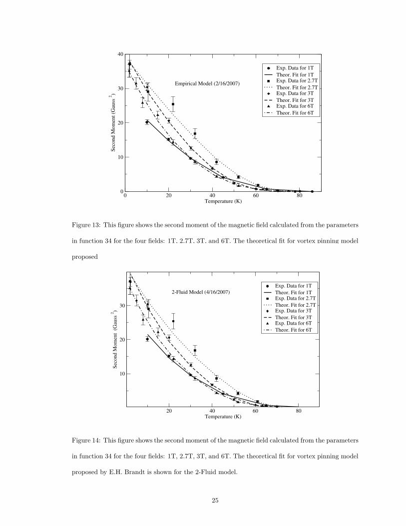
Figure 13: This figure shows the second moment of the magnetic field calculated from the parameters

in function 34 for the four fields: 1T, 2.7T, 3T, and 6T. The theoretical fit for vortex pinning model

proposed by E.H. Brandt is shown for the Empirical model.

20 40 60 80Temperature (K)

10

20

30

Sec

ond M

om

ent

(G

auss

2)

Exp. Data for 1T




Theor. Fit for 6T

2-Fluid Model (4/16/2007)



proposed by E.H. Brandt is shown for the 2-Fluid model.

25

Table 2: Parameters from the vortex pinning model using the 2-Fluid Model.


1.0 2.9 43.1 0.489 0.0417 0.426 4.28

2.7 43.1 0.0369 0.438

2.5 43.1 0.0322 0.452

2.3 43.1 0.0279 0.466

2.7 2.9 55.4 0.297 0.0549 0.501 1.60

2.7 55.4 0.0483 0.512

2.5 55.4 0.0422 0.524

2.3 55.4 0.0364 0.536

3.0 2.9 43.1 0.282 0.0560 0.529 4.46

2.7 43.1 0.0493 0.567

2.5 43.1 0.0430 0.548

2.3 43.1 0.0372 0.559

6.0 2.9 38.4 0.199 0.0519 0.477 1.08

2.7 38.4 0.0455 0.521

2.5 38.4 0.0398 0.501

2.3 38.4 0.0344 0.514

26

Table 3: ul/a and up/a; functional form bcs model (nv=0.15)


1.0 2.9 58.4 0.489 0.0197 0.187 2.21

2.7 58.4 0.0174 0.193

2.5 58.4 0.0152 0.201

2.3 58.3 0.0132 0.208

2.7 2.9 106 0.297 0.0298 0.126 1.44

2.7 106 0.0351 0.129

2.5 105 0.0306 0.133

2.3 105 0.0264 0.137

3.0 2.9 64.1 0.282 0.0443 0.133 5.85

2.7 64.1 0.0390 0.137

2.5 64.1 0.0341 0.141

2.3 64.1 0.0294 0.144

6.0 2.9 50.0 0.199 0.0283 0.0801 1.14

2.7 50.0 0.0249 0.0828

2.5 50.0 0.0217 0.0856

2.3 50.0 0.0188 0.0885

27

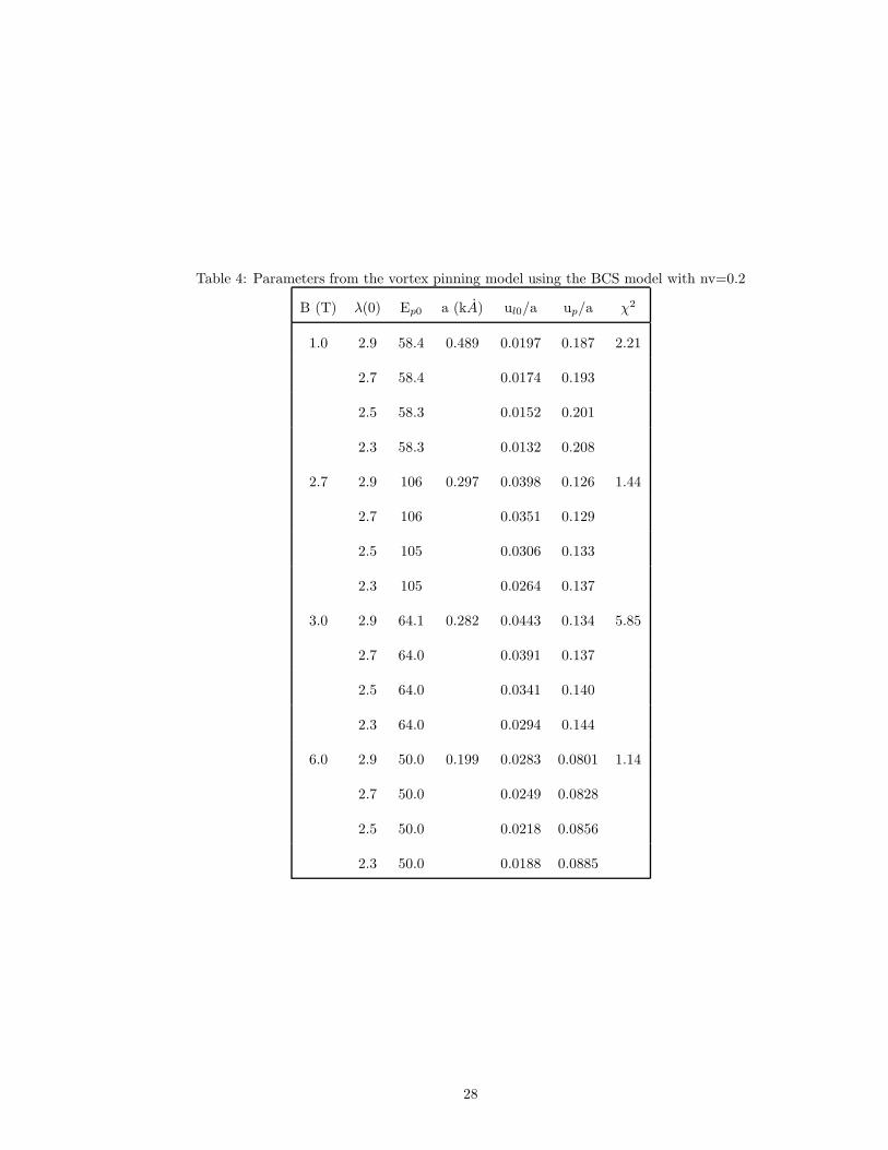
Table 4: Parameters from the vortex pinning model using the BCS model with nv=0.2


1.0 2.9 58.4 0.489 0.0197 0.187 2.21

2.7 58.4 0.0174 0.193

2.5 58.3 0.0152 0.201

2.3 58.3 0.0132 0.208

2.7 2.9 106 0.297 0.0398 0.126 1.44

2.7 106 0.0351 0.129

2.5 105 0.0306 0.133

2.3 105 0.0264 0.137

3.0 2.9 64.1 0.282 0.0443 0.134 5.85

2.7 64.0 0.0391 0.137

2.5 64.0 0.0341 0.140

2.3 64.0 0.0294 0.144

6.0 2.9 50.0 0.199 0.0283 0.0801 1.14

2.7 50.0 0.0249 0.0828

2.5 50.0 0.0218 0.0856

2.3 50.0 0.0188 0.0885

28


0

10

20

30

40

Sec

ond M

om

ent

(Gau

ss 2

)

Exp. Data for 1T




Theor. Fit for 6T

BCS Model nv=0.2 (4/19/2007)



proposed by E.H. Brandt is shown for the BCS model.


0

10

20

30

40

Sec

ond M

om

ent

(Gau

ss2)

Exp. Data for 1T




Theor. Fit for 6T

D-wave Model (4/19/2007)



proposed by E.H. Brandt is shown for the D-wave model.

29



1.0 2.9 58.3 0.489 0.0198 0.187 2.21

2.7 58.3 0.0174 0.193

2.5 58.3 0.0153 0.201

2.3 58.3 0.0132 0.208

2.7 2.9 106 0.297 0.0398 0.126 1.44

2.7 105 0.0351 0.129

2.5 105 0.0306 0.133

2.3 105 0.0264 0.137

3.0 2.9 64.1 0.282 0.0443 0.134 5.85

2.7 64.1 0.0390 0.137

2.5 64.1 0.0341 0.141

2.3 64.0 0.0294 0.144

6.0 2.9 50.0 0.199 0.0283 0.0801 1.14

2.7 50.0 0.0249 0.0828

2.5 50.0 0.0218 0.0856

2.3 50.0 0.0188 0.0885

30



1.0 2.9 58.2 0.489 0.0199 0.187 2.21

2.7 58.1 0.0176 0.194

2.5 58.1 0.0154 0.201

2.3 58.1 0.0133 0.208

2.7 2.9 105 0.297 0.0399 0.126 1.44

2.7 105 0.0351 0.129

2.5 105 0.0306 0.133

2.3 105 0.0264 0.138

3.0 2.9 64.0 0.282 0.0443 0.134 5.85

2.7 64.0 0.0391 0.137

2.5 63.9 0.0341 0.141

2.3 63.9 0.0295 0.144

6.0 2.9 49.9 0.199 0.0284 0.0801 1.14

2.7 49.9 0.0250 0.0828

2.5 49.9 0.0218 0.0856

2.3 49.9 0.0188 0.0885

31



1.0 2.9 53.6 0.489 0.0238 0.189 2.52

2.7 53.6 0.0210 0.196

2.5 53.6 0.0184 0.203

2.3 53.6 0.0159 0.210

2.7 2.9 94.1 0.297 0.0414 0.127 1.51

2.7 94.0 0.0365 0.131

2.5 93.9 0.0318 0.135

2.3 93.8 0.0275 0.139

3.0 2.9 59.1 0.282 0.0462 0.136 5.70

2.7 59.1 0.0407 0.139

2.5 59.1 0.0355 0.143

2.3 59.0 0.0307 0.146

6.0 2.9 47.4 0.199 0.0312 0.0812 1.14

2.7 47.4 0.0275 0.0839

2.5 47.4 0.0240 0.0866

2.3 47.4 0.0208 0.0895

32



1.0 2.9 52.7 0.489 0.0265 0.193 4.24

2.7 52.7 0.0233 0.199

2.5 52.7 0.0204 0.206

2.3 52.7 0.0177 0.213

2.7 2.9 80.6 0.297 0.0447 0.132 1.54

2.7 80.5 0.0393 0.135

2.5 80.5 0.0343 0.139

2.3 80.4 0.0297 0.143

3.0 2.9 53.6 0.282 0.0490 0.140 5.26

2.7 53.6 0.0432 0.143

2.5 53.6 0.0377 0.146

2.3 53.5 0.0325 0.150

6.0 2.9 45.1 0.199 0.0350 0.0830 1.12

2.7 45.1 0.0308 0.0856

2.5 45.1 0.0269 0.0883

2.3 45.1 0.0233 0.0911

33

Table 9: Parameters from the vortex pinning model using the D-wave model.


1.0 2.9 86.2 0.489 0.0359 0.186 3.66

2.7 86.2 0.0316 0.193

2.5 86.2 0.0276 0.200

2.3 86.1 0.0238 0.207

2.7 2.9 111 0.297 0.0629 0.135 1.10

2.7 111 0.0553 0.139

2.5 111 0.0483 0.143

2.3 111 0.0416 0.147

3.0 2.9 79.9 0.282 0.0628 0.136 3.18

2.7 79.9 0.0553 0.140

2.5 79.8 0.0482 0.143

2.3 79.8 0.0416 0.147

6.0 2.9 74.1 0.199 0.0496 0.0774 1.01

2.7 74.1 0.0437 0.0802

2.5 74.0 0.0381 0.0831

2.3 74.0 0.0329 0.0861

34

4 Conclusion

We have used a back-to-back heterodyned Guassian-Gaussian to fit µ-SR data. These

fits have been analyzed with a pinning model proposed by Brandt. We found that

for BSSCO displacements of type up dominate which seems reasonable considering

its pancake-like nature. We have found that the statistical difference is not large

enough to differenitiate between the different models for the penetration depth. We

cannot conclude decisively from vortex pinning whether the superconductor BSCCO

is d-wave or s-wave.

References

[1] P.G. de Gennes. Superconductivity of Metals and Alloys. Addison-Wesley Pub-

lishing Company, 1966.

[2] Charles P. Poole, Jr., Horacio A. Farach, and Richard J. Freswick. Superconduc-

tivity. Academic Press, 1995.

[3] Orest G. Vendik, Irina B. Vendik, and Dimitri I. Kaparkov. Emperical model of

the microwave properties of high-temperature superconductors. IEEE Transac-

tions on MIcrowave Theory and Techniques, 46:469–478, 1998.

[4] D. Shoenberg. Superconductivity. Cambridge University Press, 1965.

[5] Michael Tinkham. Introduction to Superconductivity. McGraw-Hill, Inc, 1996.

[6] Anderson and Morel. Phys. Rev., 123:1911, 1961.

[7] M. H. S. Amin, M. Franz, and Ian Affleck. Effective penetration depth in the

vortex state of a d-wave superconductor. Condensed Matter, 3:1–4, 2000.

35

[8] D.R. Harshman, W.J. Kossler, X. Wan, A.T. Fiory, A.J. Greer, D.R. Noakes,

C.E. Stronach, E. Koster, and John D. Dow. Nodeless pairing in single-crystal

YBa2Cu3O7. Phys. Rev. B, 69:174505, 2004.

[9] A.T. Fiory, D.R. Harshman, J. Jung, I.-Y. Isaac, W.J. Kossler, A.J. Greer, D.R.

Noakes, C.E. Stronach, E. Koster, and John D. Dow. Fluxon pinning in the node-

less pairing state of superconducting YBa2Cu3O7. Electronic Materials, 34:474–

483, 2005.

[10] E.H. Brandt. Magnetic-field variance in layered superconductors. Phys. Rev.,

66:3213–3216, 1991.

[11] W. J. Kossler and A. J. Greer. trix06, 2001.

[12] A. Yaouanc, P. Dalmas de Reotier, and E.H. Brandt. Phys. Rev. B, 55:11107,

1997.

[13] E.H. Brandt. Thermal fluctuation of the vortex positions in high-Tc supercon-

ductors. Physica C, 162-164:1167–1168, 1989.

[14] H. Suhl. Inertial mass of a moving fluxoid. Phys. Rev., 14:226–229, 1965.

[15] Neil W. Ashcroft and N. David Mermin. Solid State Physics. Saunders College,

1976.

[16] G. Blatter, M.V. Feigel’man, V.B. Geshkenbein, A.I. Larkin, and V.M. Vinokur.

Vortices in high-temperature superconductors. Reviews of Modern Physics,

66:1125–1388, 1994.

[17] Pintu Sen, S.K. Bandyopadhyay, P.M.G. Nambissan, R. Ganguly, P. Barat,

and P. Mukherjee. The study of inter and intragranular pinning be-

havior of oxygen irradiated textured polycrystalline Bi2Sr2CaCu2O8+δ and

Bi1.84Pb0.34Sr1.91Ca2.03Cu3.06O10+e. lta superconductors. Physica C: Superconduc-

tivity, 407:55–61, 2004.

36

[18] C.S. Pande and M. Suenaga. A model of flux pinning by grain boundaries in

type-II superconductors. Applied Physics Letters, 29:443–444, 1976.

37

vortex pinning in high-tc...

Documents