1  

Applying Value and Momentum across Asset Classes in a Quantitative Tactical Asset Allocation Framework

Peng Wang1

Preliminary and to be Completed

Last Updated Jan-12-2011

Abstract

We present a concise quantitative method for combining value and

momentum strategies in a tactical asset allocation framework by directly

comparing the attractiveness of valuations across a broad range of asset classes.

Our broad and diverse publicly traded asset classes include public equity,

investment grade and high yield bonds, cash, Treasury Inflation Protected

Securities (TIPS), commodity and real estate. We refine the basic yield

approach to valuation by standardizing the value signal using the Z-score. By

tactically adjusting the weight of each asset class based on its perceived value

and momentum signals, our model shows significant improvement in overall

portfolio performance.

Introduction

Clifford S. Asness et al. have documented in their 2008 paper “Value and

Momentum Everywhere” that value and momentum deliver abnormal positive

expected returns in a variety of markets and asset classes at the security level

(Asness, Moskowitz, & Pedersen). The key issue we address here is whether

such effect can also be observed across asset classes at the index level in a

tactical asset allocation framework. More specifically, we want to examine

                                                            1 Peng Wang, Georgetown University Investment Office, 202-390-5676, pw35@georgetown.edu

2  

whether we can improve on a given strategic asset allocation by tactically

adjusting the weights of asset classes based on their perceived value and

momentum attractiveness. The strategic asset allocation here is a

representative mix of a broad and diversified seven (7) asset classes, including

world equity, investment grade bond, high yield bond, cash, TIPS, commodity

and real estate. For practitioners, our model provides a dynamic top-down

approach to tactical asset allocation in accordance with the ever-changing

market environments.

Data and Methodology

Table 1 is an overview of the seven asset classes that set up the framework

for our analyses and the indices that we used to measure the value and

momentum signals. The selection of the asset classes is not based on a formal

set of rules. In fact, each asset class should provide a unique set of return and

risk characteristics so that a portfolio of the asset classes would provide

diversification and reduce the overall risk. More specifically, investments

should provide growth as well as protection against both deflation and inflation

risks most institutional investors face. Existing literature suggests that high yield,

commodities and real estate add most value to the traditional asset mix of

stocks, bonds and cash (Mars, Robeco, & Rabobank, Ocotober 2009). Equity

would provide growth and include both U.S and non-U.S. equity, as the

distinction between the two has lost some of its meaning over time. Fixed

income performs better than equity in a deflationary or weak economic

environment and is a portfolio of the three unique return/risk characteristics

for the asset class –investment grade (yield curve risk), high yield (credit risk)

and cash (no risk). Inflation-hedging or real assets include a basket of assets

3  

that will protect against inflation over a long period. TIPS offers good inflation

protection with lowest risk since they are U.S government bonds. Other real

assets including commodities and real estate protect investor during an

inflationary regime.

Table 1 - Asset Classes and Indices

Asset Class Index

Equity Global Equity MSCI ACWI

Investment Grade Barclays Agg.

Fixed Income High Yield MLHY II

Cash T-Bill

TIPS 10yr on-the-run TIPS

Real Asset Commodity GSCI

Real Estate NAREIT

The indices that we use to represent our seven asset classes are (table 1):

the Morgan Stanley Capital International ACWI Index (MSCI ACWI), Barclays

Capital Aggregate Bond Index (Barclays Agg.) gross return, Merrill Lynch High

Yield Master II (MLHY II) total return, Merrill Lynch 91-Day Treasury (Cash),

10 year on the run Treasury Inflation-Protected Securities (TIPS), Goldman

Sachs Commodity Index (GSCI) total return, and National Association of Real

Estate Investment Trusts Index (NAREIT) global total return.

It is comparatively easy to apply momentum strategy to cross-asset

allocation since it only requires past prices as inputs. We use the return based

on last month price over a simple moving average (SMA) of trailing 12-month-

4  

ending prices2 for the momentum signal. We consider such momentum signal

negative if the return is negative. The SMA offers a smoothing mechanics on

the momentum signals. Previous study also shows that a trend-following SMA

model could increase risk-adjusted returns (Faber, Februrary 2009).

It is less straightforward to construct a cross-asset allocation value

strategy, because no obvious valuation measure is applicable to every asset class.

The starting point of our approach is a simple yield measure for each asset class

(Blitz & Van Vliet, 2008). We use the book-to-price (B/P) for equity assets,

cash-flow-to-price for REITs, and the standard yield-to-maturity for all the

bond assets, including investment grade, high-yield, cash and TIPS. For

commodity, we use a backwardation-contango measurement, defined by (next

month futures price - current month futures price)/next month futures price. If

such signal is negative, it is in contango; and vice versa, if it is positive, it is in

backwardation. Backwardation is a value situation because of the roll-yield. All

valuation data are from 1986 January3 except TIPS from 1997 March. The

yields on T-Bill and TIPS are from Federal Reserve System; Cash-flow/Price

for NAREIT is based on Goldman Sachs respective US REIT universe4. The

backwardation/contango signal is calculated from GSCI generic futures prices

from Bloomberg.

All the above valuation measurements share the same feature that the

bigger the value, the more attractive the valuation. Obviously, it is less

meaningful to directly compare our basic yield measurement of equity (B/P) to

investment grade (yield), or the yield of investment grade to that of high yield.

In order to compare the value measurement meaningfully across asset classes

                                                            2 One can also use 10-month, 6-month, 3-month and so on. For simplicity we just use 12-month as an example. 3 Valuation data for emerging market started in Jan-86. 4 The use of NAV-to-price data based on UBS respective of US REIT universe will not change our conclusions.

5  

and account for the inherited structural difference, we refine our basic yield

approach by standardizing the value signal. We calculate the Z-score at any

given month t, using its entire historical data up to month t, based on the

following formula:

,

,

Such Z-score, measuring how far the signal is away from its historical

mean in terms of how many standard deviations in between, offers a direct way

to compare the attractiveness of valuation of different asset classes and

provides insights to the allocation for month t+1.

It is also worth noting that for both value and momentum

measurements, we only use historical data up to any given time t, in order to

avoid forward-looking bias.

The Quantitative System

We analyze the performance based on two (2) sets of policy/base

weights. One is equal weighted. The other is a set of hypothetical weights,

which serves more conventionally to institutional investors. Since TIPS is not

introduced until early 1997, we have six (6) asset classes before March-1998 and

seven (7) asset classes including TIPS after5. Table 2 provides an overview of

the two policy benchmark weights.

                                                            5 Ensure 12 months of return data for the momentum strategy for TIPS.

6  

Table 2 - Benchmark Weights

Global

Equity

Investment

Grade

High

Yield Cash TIPs Commodity

Real

Estate

Equal

before 1998/03 1/6 1/6 1/6 1/6 0 1/6 1/6

after 1998/03 1/7 1/7 1/7 1/7 1/7 1/7 1/7

Hypothetical

before 1998/03 45.67% 18.17% 11.17 7.67% 0 8.67% 8.67%

after 1998/03 45.0% 17.5% 10.5% 7.0% 4.0% 8.0% 8.0%

We first examine momentum and value strategy separately and then

combine them with trend-following model in the tactical allocation framework.

Momentum - At the end of every month, we rank our seven asset classes

based on their momentum signal. The ranking is used to adjust the asset class

weights from the policy or base weight. For asset class i, the momentum

suggested weights are:

Where R is the adjusting basis, a parameter we can change. For now, we set R

= 2%, which will satisfy the fully-invested, no-leverage and no-short constraints

and result in very small deviations from the benchmarks. For the case of seven

asset classes, the average rank is equal to 4. In this way, the summation of the

weights will keep unchanged after the adjustment.

7  

Value – Following the same idea, each month we look at the value

measurements, i.e. the Z-scores, to identify any asset class that is significantly

under/over-valued and take advantage of the long-term mean-reversion

mechanism. Meantime, as an effort to avoid “value trap,” we only increase the

weight of the undervalued asset class with a Z-score above 2. Consistently, we

also only reduce exposure to the overvalued asset class with a Z-score below -2.

Please keep in mind that the bigger the Z-score, the more attractive the

valuation is. In other words, we identify any asset class whose valuation is at

least two-standard-deviation cheaper/more expensive than its historical mean.

The asset class with a Z score between -2 and 2 will be treated as 0. Just as

momentum strategy, we use ranking to adjust the asset class weights from the

policy weights. Asset classes with the same Z-score (0) will have the same rank.

We combine momentum and value strategy with the trend-following

model as shown in Exhibit 1.

Exhibit 1

Step 1 (Momentum): Each month, we first apply the momentum strategy to

calculate Wm.

Step 2 (Trend following - optional): We could then follow a simple trend

following the model developed by M.T. Faber (Faber, Februrary 2009). If any

Base Momentum WmTrend-

Following Wmt Value Wmtv

8  

asset class has a negative momentum, we reduce its holding to zero and put it

into cash. This step will increase risk-adjusted return (higher Sharpe Ratio) but

decrease the information ratio as it will significantly increase tracking error. We

recommend this step for hedge fund type managers who care more about

absolute performance measurements.

0%,

Step 3 (Value): We first find overvalued asset classes with Z <-2 and reduce

the exposures to zero and increase the corresponding amount to cash6. We

subsequently identify undervalued asset classes with Z score above 2. We

reduce our cash holding from former step(s) to zero and equally increase our

exposures to those asset classes with attractive valuations. The weights will not

be adjusted if we do not identify any over/under-valued asset class.

0%, 2

: 2

, 2

0%

                                                            6 Instead, one can chose to only invest in undervalued (Z > 2) asset classes, but not reduce exposure to overvalued ones; similarly this step will improve Sharpe ratio but reduce information ratio as it increases tracking error.

9  

Preliminary Results and Robustness Test

The main results are presented in Table 3-5. E and H stand for the

equal-weighted and the hypothetical benchmark portfolios respectively. The

strategy applied to the benchmark portfolios is noted in the brackets. “V” and

“M” stands for the value strategy and the momentum strategy. “MT” means

combining momentum strategy with the trend following model. “M&V”

combines value and momentum without step 2, while “MT&V” includes both

step 2 and 3. An annual risk free rate of 4% is used for Sharpe Ratio analysis.

Testing period is from 1989 January7 to 2010 September.

We examined the robustness of our findings and computed alpha, beta

and T-stat for each strategy against its policy benchmark from monthly return

data. The monthly risk-free rate is downloaded from Fama/French website. We

also examine if step 2 and 3 in the combined model has generated alpha by

using intermediate results as benchmark, i.e. use M only as benchmark for MT

and MT as benchmark for MT&V.

                                                            7 Total return data for ACWI is from Dec-1988 on Bloomberg.

10  

Table 3a - Annual Returns (as of 9/30/2010)

Annual Returns

E E(V) E(M) E(M&V) E(MT) E(MT&V)

2010 YTD 6.24% 6.74% 5.41% 6.43% 3.16% 5.69%

2009 22.35% 26.03% 23.58% 29.02% 13.84% 28.67%

2008 -21.83% -19.05% -17.62% -18.21% -0.59% -3.86%

2007 7.60% 7.60% 8.20% 8.77% 8.30% 8.87%

2006 8.47% 8.47% 11.05% 12.80% 11.46% 11.92%

2005 8.93% 8.93% 8.29% 8.29% 8.29% 8.29%

2004 13.12% 13.12% 14.29% 14.49% 14.24% 14.44%

2003 19.11% 17.82% 20.95% 18.23% 19.46% 15.51%

2002 6.02% 5.90% 7.64% 8.43% 7.29% 9.98%

2001 -2.27% -0.48% 0.11% 1.38% 3.39% 6.58%

2000 11.53% 12.92% 14.58% 20.35% 14.91% 22.96%

1999 9.55% 7.77% 9.85% 6.08% 8.36% 3.94%

1998 -2.71% -2.47% -0.58% 1.72% 4.01% 7.48%

1997 7.76% 7.76% 7.87% 10.17% 8.32% 10.63%

1996 16.31% 16.32% 18.38% 18.66% 18.38% 18.66%

1995 16.31% 16.35% 16.15% 16.77% 15.19% 15.76%

1994 2.11% 2.09% 1.08% 0.52% 1.28% 1.35%

1993 9.46% 9.46% 11.48% 11.48% 13.12% 13.12%

1992 6.69% 6.69% 7.84% 7.84% 7.14% 7.14%

1991 17.56% 19.13% 15.90% 18.90% 10.27% 16.54%

1990 1.37% -0.54% 3.17% 0.47% 9.39% 1.93%

11  

Table 3b - Annual Returns (as of 9/30/2010)

Annual Returns

H H(V) H(M) H(M&V) H(MT) H(MT&V)

2010 YTD 5.93% 6.42% 5.09% 5.49% -0.98% 2.83%

2009 27.09% 30.90% 28.46% 31.10% 15.26% 33.26%

2008 -28.58% -26.02% -24.67% -24.99% -4.94% -8.46%

2007 9.08% 9.08% 9.69% 10.10% 9.61% 10.01%

2006 13.26% 13.26% 15.92% 16.57% 16.00% 16.32%

2005 9.40% 9.40% 8.74% 8.74% 8.74% 8.74%

2004 13.55% 13.55% 14.74% 14.78% 14.68% 14.71%

2003 24.12% 22.79% 26.10% 24.66% 21.57% 17.26%

2002 -3.41% -3.53% -1.82% -1.50% 5.64% 9.48%

2001 -7.20% -5.48% -4.88% -4.33% 3.73% 7.71%

2000 0.65% 1.92% 3.44% 13.49% 6.82% 19.12%

1999 14.25% 12.41% 14.55% 5.72% 14.32% 4.76%

1998 6.37% 6.65% 8.64% 13.56% 5.92% 12.45%

1997 10.16% 10.16% 10.23% 16.10% 10.38% 16.25%

1996 13.08% 13.09% 15.10% 15.14% 15.10% 15.14%

1995 17.02% 17.07% 16.85% 16.39% 15.78% 14.68%

1994 1.86% 1.85% 0.83% 0.60% 1.55% 4.10%

1993 14.38% 14.38% 16.48% 16.48% 16.26% 16.26%

1992 1.93% 1.93% 3.04% 3.04% 1.81% 1.81%

1991 18.00% 19.56% 16.35% 17.80% 7.78% 14.95%

1990 -5.64% -7.54% -3.80% -5.08% 4.54% -3.72%

12  

Table 4a – Return and Risk R = 2% (as of 12/31/2009)

Annualized Returns

Years E E(V) E(M) E(M&V) E(MT) E(MT&V)

1 yr 22.35% 26.03% 23.58% 29.02% 13.84% 28.67%

3 yr 0.96% 3.16% 3.28% 4.71% 7.02% 10.43%

5 yr 3.99% 5.34% 5.79% 7.00% 8.15% 10.30%

7 yr 16.51% 17.66% 20.16% 22.17% 23.05% 26.80%

10 yr 6.59% 7.48% 8.50% 9.64% 9.91% 12.02%

15yr 7.46% 7.96% 9.04% 9.93% 10.19% 11.73%

20yr 7.41% 7.76% 8.72% 9.35% 9.68% 10.75% Volatilities

Years E E(V) E(M) E(M&V) E(MT) E(MT&V)

1 yr 12.82% 12.95% 10.30% 12.20% 4.24% 10.45%

3 yr 13.81% 13.15% 12.12% 13.27% 5.25% 8.97%

5 yr 11.11% 10.60% 10.04% 10.87% 5.32% 7.74%

7 yr 9.87% 9.47% 9.17% 9.84% 5.65% 7.59%

10 yr 8.74% 8.36% 8.09% 8.66% 5.15% 6.75%

15yr 7.73% 7.46% 7.26% 7.63% 4.92% 6.36%

20yr 7.13% 6.96% 6.76% 7.13% 4.91% 6.12%

Sharpe Ratio8

Years E E(V) E(M) E(M&V) E(MT) E(MT&V)

1 yr 1.43 1.70 1.90 2.05 2.32 2.36

3 yr -0.22 -0.06 -0.06 0.05 0.57 0.72

5 yr 0.00 0.13 0.18 0.28 0.78 0.81

7 yr 1.27 1.44 1.76 1.85 3.37 3.00

10 yr 0.30 0.42 0.56 0.65 1.15 1.19

15yr 0.45 0.53 0.69 0.78 1.26 1.22

20yr 0.48 0.54 0.70 0.75 1.16 1.10

                                                            8 4% risk-free rate is used for Sharpe Ratio calculation.

Maximum Drawdown

E E(V) E(M) E(M&V) E(MT) E(MT&V)

33.50% 29.95% 28.61% 29.27% 6.77% 13.20%

13  

Table 4b - Return and Risk R = 2% (as of 12/31/2009)

                                                            9 4% risk-free rate is used for Sharpe Ratio calculation.

Annualized Returns

Years H H(V) H(M) H(M&V) H(MT) H(MT&V)

1 yr 27.09% 30.90% 28.46% 31.10% 15.26% 33.26%

3 yr -0.33% 1.85% 2.01% 2.68% 6.29% 10.30%

5 yr 4.17% 5.53% 6.00% 6.54% 8.66% 11.16%

7 yr 15.25% 16.41% 18.91% 21.07% 23.28% 28.69%

10 yr 4.55% 5.43% 6.46% 7.70% 9.47% 12.36%

15yr 7.01% 7.52% 8.61% 9.54% 10.39% 12.43%

20yr 6.69% 7.03% 8.02% 8.69% 9.34% 10.89% Volatilities

Years H H(V) H(M) H(M&V) H(MT) H(MT&V) 1 yr 15.92% 16.05% 13.43% 14.59% 5.04% 11.27%3 yr 16.07% 15.51% 14.38% 15.07% 6.04% 9.86% 5 yr 12.96% 12.51% 11.90% 12.39% 6.19% 8.61% 7 yr 11.49% 11.13% 10.66% 11.06% 6.07% 8.22% 10 yr 10.86% 10.51% 10.01% 10.23% 5.75% 7.31% 15yr 9.77% 9.50% 9.20% 8.89% 6.15% 6.90% 20yr 9.30% 9.20% 8.76% 8.58% 6.12% 6.89%

Sharpe Ratio9

Years H H(V) H(M) H(M&V) H(MT) H(MT&V)

1 yr 1.45 1.68 1.82 1.86 2.24 2.60

3 yr -0.27 -0.14 -0.14 -0.09 0.38 0.64

5 yr 0.01 0.12 0.17 0.20 0.75 0.83

7 yr 0.98 1.11 1.40 1.54 3.17 3.00

10 yr 0.05 0.14 0.25 0.36 0.95 1.14

15yr 0.31 0.37 0.50 0.62 1.04 1.22

20yr 0.29 0.33 0.46 0.55 0.87 1.00

Maximum Drawdown

H H(V) H(M) H(M&V) H(MT) H(MT&V)

39.11% 32.45% 34.16% 34.71% 7.61% 14.40%

14  

Table 5a – Alpha and Tracking Error R = 2% (as of 12/31/2009)

Alpha

Years E(V) E(M) E(M&V) E(MT) E(MT&V)

1 yr 3.69% 1.23% 6.68% -8.51% 6.33%

3 yr 2.20% 2.32% 3.75% 6.06% 9.48%

5 yr 1.35% 1.80% 3.01% 4.16% 6.31%

7 yr 1.15% 3.65% 5.66% 6.55% 10.29%

10 yr 0.89% 1.91% 3.05% 3.32% 5.42%

15yr 0.50% 1.58% 2.47% 2.73% 4.27%

20yr 0.34% 1.30% 1.93% 2.26% 3.33%

Tracking Error

Years E(V) E(M) E(M&V) E(MT) E(MT&V)

1 yr 1.16% 3.02% 1.95% 12.26% 4.57%

3 yr 1.35% 2.73% 2.15% 12.39% 8.18%

5 yr 1.08% 2.34% 2.08% 9.70% 6.57%

7 yr 1.01% 2.16% 2.27% 8.31% 5.99%

10 yr 0.95% 2.02% 2.27% 7.27% 5.48%

15yr 0.86% 1.76% 2.24% 6.12% 5.02%

20yr 0.94% 1.68% 2.03% 5.62% 4.55%

Info Ratio

Years E(V) E(M) E(M&V) E(MT) E(MT&V)

1 yr 3.17 0.41 3.43 -0.69 1.39

3 yr 1.63 0.85 1.74 0.49 1.16

5 yr 1.25 0.77 1.44 0.43 0.96

7 yr 1.14 1.69 2.49 0.79 1.72

10 yr 0.94 0.95 1.35 0.46 0.99

15yr 0.58 0.90 1.10 0.45 0.85

20yr 0.36 0.78 0.95 0.40 0.73

15  

Table 5b – Annual Alpha and Tracking Error R = 2% (as of 12/31/2009)

Alpha

Years H(V) H(M) H(M&V) H(MT) H(MT&V)

1 yr 3.81% 1.37% 4.01% -11.83% 6.17%

3 yr 2.18% 2.34% 3.01% 6.62% 10.63%

5 yr 1.36% 1.82% 2.36% 4.49% 6.99%

7 yr 1.16% 3.66% 5.82% 8.03% 13.44%

10 yr 0.88% 1.91% 3.15% 4.93% 7.81%

15yr 0.50% 1.60% 2.53% 3.37% 5.42%

20yr 0.34% 1.32% 2.00% 2.64% 4.20%

Tracking Error

Years H(V) H(M) H(M&V) H(MT) H(MT&V)

1 yr 1.16% 3.02% 2.00% 15.26% 6.65%

3 yr 1.35% 2.73% 2.19% 14.08% 9.34%

5 yr 1.08% 2.34% 2.00% 10.98% 7.41%

7 yr 1.01% 2.16% 2.00% 9.61% 7.07%

10 yr 0.95% 2.02% 2.98% 9.13% 7.64%

15yr 0.86% 1.76% 3.70% 7.59% 7.23%

20yr 0.94% 1.68% 3.25% 7.22% 6.58%

Info Ratio

Years H(V) H(M) H(M&V) H(MT) H(MT&V)

1 yr 3.28 0.45 2.01 -0.77 0.93

3 yr 1.62 0.85 1.37 0.47 1.14

5 yr 1.26 0.78 1.18 0.41 0.94

7 yr 1.15 1.69 2.91 0.84 1.90

10 yr 0.93 0.95 1.06 0.54 1.02

15yr 0.58 0.90 0.68 0.44 0.75

20yr 0.36 0.79 0.61 0.37 0.64

16  

Table 6a – Robustness Test

Strategy Benchmark alpha T-Stat Beta T-Stat

E(V) E 0.03% 2.10 0.97 125.12

E(M) E 0.11% 3.97 0.93 67.54

E(M&V) E 0.15% 4.23 0.97 56.45

E(MT) E 0.32% 4.54 0.47 13.75

E(MT&V) E 0.33% 4.79 0.69 20.76

H(V) H 0.03% 1.76 0.99 164.71

H(M) H 0.11% 3.96 0.94 91.49

H(M&V) H 0.17% 3.31 0.88 45.26

H(MT) H 0.31% 3.54 0.45 14.06

H(MT&V) H 0.40% 4.56 0.56 17.24

Table 6b - Robustness Test with Intermediate Steps

Strategy Benchmark alpha T-Stat Beta T-Stat

E(MT) E(M) 0.23% 3.90 0.59 20.56

E(MT&V) E(MT) 0.12% 1.78 0.94 18.99

H(MT) H(M) 0.23% 3.03 0.54 18.31

H(MT&V) H(MT) 0.21% 2.30 0.82 17.14

Our model shows improved overall performance based on both

benchmark portfolios. Value and momentum alone will both generate

significant alpha10. By nature, momentum strategy will adjust weights every

month. Meanwhile, value strategy was triggered 149 months out of the total

261 months test period with a critical Z score of two(2)11. We also see that the

simple equal-weighted portfolio offers better diversification and risk-adjusted

return (higher Sharpe Ratio) than the more conventional equity heavy

allocation (the hypothetical portfolio) in the long run (Maillard, Roncalli, &

Teiletche, May 2009). The trend following mechanism (step 2) acts as hedging

by moving capital to cash, and improves the risk-adjusted return in the long run

                                                            10 For our sample, the critical value of t is about 1.65. 11 Out of the 261 months, there are 149 months when one or more asset classes have a Z score less than -2 or bigger than 2. This is also a parameter that can be changed. A smaller threshold will obviously

17  

because of capital preservation. The maximum drawdown is reduced by more

than 20% in our framework. However, momentum combined with trend

following may not do as well at market turns, e.g.2009. Further adding the

value strategy (step 3) could help to identify the opportunity to participate in

the market rally (see exhibit 2).

18  

Exhibit 2 – Growth of One Dollar

0123456789

10

1/1/

1989

12/1

/198

911

/1/1

990

10/1

/199

19/

1/19

928/

1/19

937/

1/19

946/

1/19

955/

1/19

964/

1/19

973/

1/19

982/

1/19

991/

1/20

0012

/1/2

000

11/1

/200

110

/1/2

002

9/1/

2003

8/1/

2004

7/1/

2005

6/1/

2006

5/1/

2007

4/1/

2008

3/1/

2009

2/1/

2010

E E(M) E(MT) E(MT&V)

0123456789

10

1/1/

1989

12/1

/198

911

/1/1

990

10/1

/199

19/

1/19

928/

1/19

937/

1/19

946/

1/19

955/

1/19

964/

1/19

973/

1/19

982/

1/19

991/

1/20

0012

/1/2

000

11/1

/200

110

/1/2

002

9/1/

2003

8/1/

2004

7/1/

2005

6/1/

2006

5/1/

2007

4/1/

2008

3/1/

2009

2/1/

2010

H H(M) H(MT) H(MT&V)

19  

The effect of R can be demonstrated through a simple example. We look

at the 20-year Sharpe Ratio of the combined model on the equally-weighted

benchmark portfolio. As we increase R, we need to relax the no-short no-

leverage constraint and the Sharpe ratio is optimized around R = 7% with a

value of 1.18. Under the no-short constraint, the maximum value allowed for R

is about 4.76%, which gives a 20-year Sharpe ratio about 1.1712.

Exhibit 3 - Sharpe Ratio VS R

 

 

                                                            12 The same analysis can be done on the information ratio. However, the 20-year information ratio saturates faster than Sharpe Ratio on R and is optimized at a smaller value of 2%. This is because the tracking error increases faster as the weights deviate bigger away from the policy benchmark.

1

1.02

1.04

1.06

1.08

1.1

1.12

1.14

1.16

1.18

1.2

0 0.01 0.02 0.03 0.04 0.05 0.06 0.07 0.08 0.09 0.1 0.11 0.12 0.13 0.14 0.15 0.16

20yr

Sh

arp

e R

atio

R

Sharpe Ratio VS R E(MT&V)

20  

Exhibit 4 – Weight Evolution with E (MT&V)

0%

10%

20%

30%

40%

50%

60%

70%

80%

90%

100%

1/1/

1989

11/1

/198

9

9/1/

1990

7/1/

1991

5/1/

1992

3/1/

1993

1/1/

1994

11/1

/199

4

9/1/

1995

7/1/

1996

5/1/

1997

3/1/

1998

1/1/

1999

11/1

/199

9

9/1/

2000

7/1/

2001

5/1/

2002

3/1/

2003

1/1/

2004

11/1

/200

4

9/1/

2005

7/1/

2006

5/1/

2007

3/1/

2008

1/1/

2009

11/1

/200

9

9/1/

2010

MSCI ACWI Barclays Agg. High Yield Cash TIPS GSCI REITs

21  

Table 7 - Tactical allocation based on E (MT & V) R = 2%

Global Equity Investment Grade High Yield Cash TIPs Commodity Real Estate

9/1/2010 0.00% 16.29% 18.29% 30.86% 14.29% 0.00% 20.29%

8/1/2010 12.29% 16.29% 18.29% 18.57% 14.29% 0.00% 20.29%

7/1/2010 30.86% 16.29% 20.29% 0.00% 18.29% 0.00% 14.29%

6/1/2010 0.00% 14.29% 18.29% 30.86% 16.29% 0.00% 20.29%

5/1/2010 16.29% 10.29% 18.29% 8.29% 12.29% 14.29% 20.29%

4/1/2010 16.29% 12.29% 18.29% 8.29% 10.29% 14.29% 20.29%

3/1/2010 16.29% 12.29% 18.29% 8.29% 10.29% 14.29% 20.29%

2/1/2010 16.29% 12.29% 18.29% 8.29% 14.29% 10.29% 20.29%

1/1/2010 16.29% 10.29% 18.29% 8.29% 12.29% 14.29% 20.29%

12/1/2009 16.29% 10.29% 18.29% 8.29% 12.29% 14.29% 20.29%

11/1/2009 18.29% 10.29% 20.29% 8.29% 12.29% 14.29% 16.29%

10/1/2009 18.29% 12.29% 20.29% 18.57% 14.29% 0.00% 16.29%

9/1/2009 18.29% 14.29% 20.29% 18.57% 12.29% 0.00% 16.29%

8/1/2009 18.29% 16.29% 20.29% 30.86% 14.29% 0.00% 0.00%

7/1/2009 15.05% 33.33% 35.33% 0.00% 16.29% 0.00% 0.00%

6/1/2009 15.05% 33.33% 35.33% 0.00% 16.29% 0.00% 0.00%

5/1/2009 15.71% 36.00% 30.00% 0.00% 18.29% 0.00% 0.00%

4/1/2009 15.36% 35.64% 15.36% 0.00% 18.29% 0.00% 15.36%

3/1/2009 19.93% 40.21% 19.93% 0.00% 0.00% 0.00% 19.93%

2/1/2009 26.57% 46.86% 26.57% 0.00% 0.00% 0.00% 0.00%

1/1/2009 26.57% 46.86% 26.57% 0.00% 0.00% 0.00% 0.00%

12/1/2008 27.24% 45.52% 27.24% 0.00% 0.00% 0.00% 0.00%

11/1/2008 33.33% 33.33% 33.33% 0.00% 0.00% 0.00% 0.00%

10/1/2008 0.00% 100.00% 0.00% 0.00% 0.00% 0.00% 0.00%

22  

9/1/2008 0.00% 61.43% 0.00% 0.00% 18.29% 20.29% 0.00%

8/1/2008 0.00% 61.43% 0.00% 0.00% 18.29% 20.29% 0.00%

7/1/2008 0.00% 16.29% 0.00% 45.14% 18.29% 20.29% 0.00%

6/1/2008 8.29% 16.29% 14.29% 12.29% 18.29% 20.29% 10.29%

5/1/2008 0.00% 49.14% 12.29% 0.00% 18.29% 20.29% 0.00%

4/1/2008 0.00% 61.43% 0.00% 0.00% 18.29% 20.29% 0.00%

3/1/2008 0.00% 61.43% 0.00% 0.00% 18.29% 20.29% 0.00%

2/1/2008 0.00% 16.29% 0.00% 45.14% 18.29% 20.29% 0.00%

1/1/2008 14.29% 16.29% 0.00% 30.86% 18.29% 20.29% 0.00%

12/1/2007 16.29% 14.29% 0.00% 30.86% 18.29% 20.29% 0.00%

  

23  

Implementation through ETFs

All the seven asset classes have corresponding ETFs, listed in Table 8.

We try to pick ETFs with low cost and better liquidity13.

Table 8 - ETFs

Asset Class ETF Mgr/Issue Exp bps

Global Equity ACWI BlackRock 35

Investment Grade AGG BlackRock 24

High Yield JNK SSgA 40

Cash - - -

TIPS TIP BlackRock 20

Commodity GSP Barclays 75

Real Estate VNQ Vanguard 13

 

Following the same methods, we still use the index data as inputs, but

use real ETF returns to calculate performances. We compare the model’s

performances with our benchmark index14 returns, ETF returns15 and sample

performances of about 200 foundations and endowments in the BNY Mellow

Trust Universes.

                                                            13 JNK, in fact, tracks the price and yield performance of the Barclays Capital High Yield Very Liquid Index. 14 See table 1. 15 Since the inception of ACWI is 2008/04, the performances using all ETFs only have about 2 year track record. 

24  

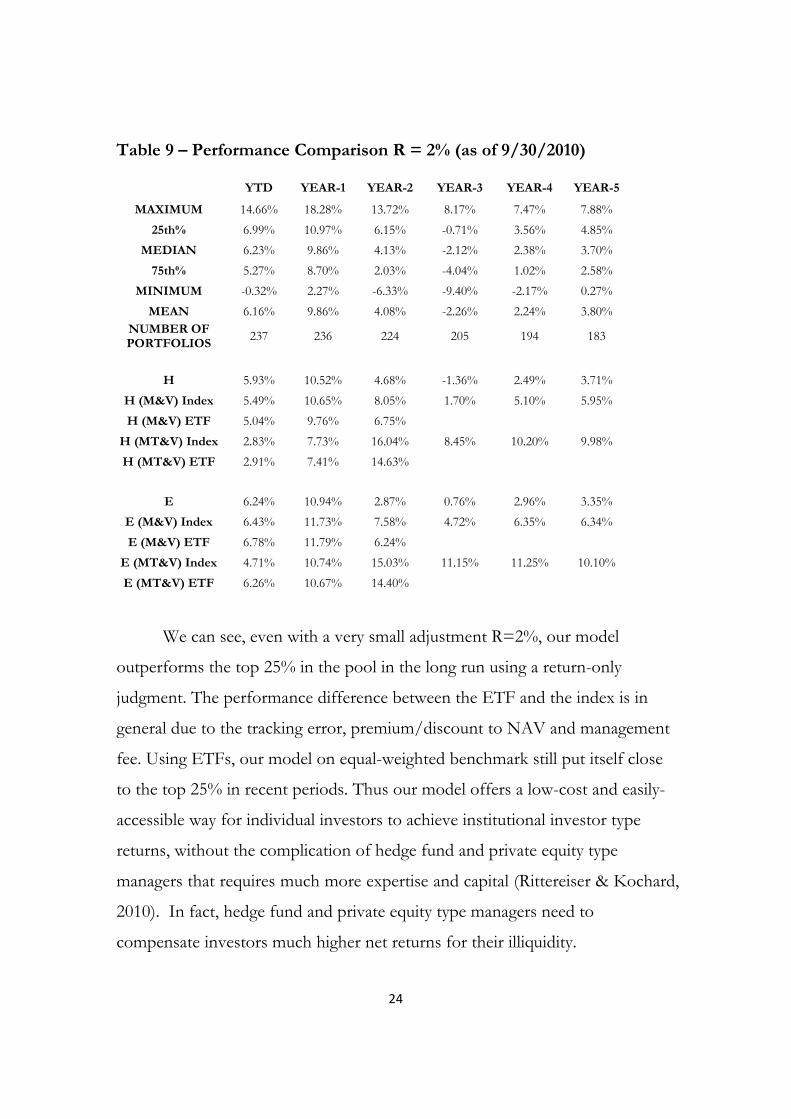
Table 9 – Performance Comparison R = 2% (as of 9/30/2010)

YTD YEAR-1 YEAR-2 YEAR-3 YEAR-4 YEAR-5

MAXIMUM 14.66% 18.28% 13.72% 8.17% 7.47% 7.88%

25th% 6.99% 10.97% 6.15% -0.71% 3.56% 4.85%

MEDIAN 6.23% 9.86% 4.13% -2.12% 2.38% 3.70%

75th% 5.27% 8.70% 2.03% -4.04% 1.02% 2.58%

MINIMUM -0.32% 2.27% -6.33% -9.40% -2.17% 0.27%

MEAN 6.16% 9.86% 4.08% -2.26% 2.24% 3.80% NUMBER OF PORTFOLIOS

237 236 224 205 194 183

H 5.93% 10.52% 4.68% -1.36% 2.49% 3.71%

H (M&V) Index 5.49% 10.65% 8.05% 1.70% 5.10% 5.95%

H (M&V) ETF 5.04% 9.76% 6.75%

H (MT&V) Index 2.83% 7.73% 16.04% 8.45% 10.20% 9.98%

H (MT&V) ETF 2.91% 7.41% 14.63%

E 6.24% 10.94% 2.87% 0.76% 2.96% 3.35%

E (M&V) Index 6.43% 11.73% 7.58% 4.72% 6.35% 6.34%

E (M&V) ETF 6.78% 11.79% 6.24%

E (MT&V) Index 4.71% 10.74% 15.03% 11.15% 11.25% 10.10%

E (MT&V) ETF 6.26% 10.67% 14.40%

 

We can see, even with a very small adjustment R=2%, our model

outperforms the top 25% in the pool in the long run using a return-only

judgment. The performance difference between the ETF and the index is in

general due to the tracking error, premium/discount to NAV and management

fee. Using ETFs, our model on equal-weighted benchmark still put itself close

to the top 25% in recent periods. Thus our model offers a low-cost and easily-

accessible way for individual investors to achieve institutional investor type

returns, without the complication of hedge fund and private equity type

managers that requires much more expertise and capital (Rittereiser & Kochard,

2010). In fact, hedge fund and private equity type managers need to

compensate investors much higher net returns for their illiquidity.

25  

We need to be careful about the liquidity constraint and the transaction

cost of our model. Some ETFs can be very illiquid and have high market

impact cost. However, with the fast growing popularity of ETFs, we may find

better, cheaper and more liquid ETFs to replace or add to the ones here for

each of the asset class to solve the issue.

Conclusion

Our strategy is basic by design, and the results are significant. Meanwhile,

further considerations and care must be taken on this instructive model before

implementation, such as liquidity constraint, transaction cost, tax and so on.

Several improvements can also be done. For example, we could seek to add the

benefit from active stock picking by using information from hedge fund’s 13F16

and 13D17. Other indicators of market risk (Sullivan, Peterson, & Waltenbaugh,

2010) can also be tested for market-timing.

Bibliography

Asness, C. S., Moskowitz, T. J., & Pedersen, L. H. (n.d.). Value and Momentum Everywhere.

Blitz, D. C., & Van Vliet, P. (2008). Global Tactical Cross-Asset Allocation: Applying Value and Momentum Across Asset Classes. The Journal of Portfolio Management .

Faber, M. T. (Februrary 2009). A Quantitative Approach to Tactical Asset Allocation. The Journal of Wealth Management .

                                                            16 Required by SEC, hedge funds need to report their quarter ending long positions within 45 days. 17 The form is required when a person or group acquires more than 5% of any class of a company's shares. This information must be disclosed within 10 days of the transaction.

26  

Maillard, S., Roncalli, T., & Teiletche, J. (May 2009). On the properties of equally-weighted risk contribution portfolios.

Mars, N. B., Robeco, R. Q., & Rabobank, T. W. (Ocotober 2009). Strategic Asset Allocation: Determining the Optimal Portfolio with Ten Asset Classes.

Rittereiser, C. M., & Kochard, L. E. (2010). Top hedge fund investors: Stories, Strategies, and Advice. Wiley Finance.

Sullivan, R. D., Peterson, S. P., & Waltenbaugh, D. T. (2010). Measuring global systemic risk: what are market saying about risk? Journal of Portfolio Management , 67.