warm dark matter chills out: constraints on the halo mass
TRANSCRIPT

MNRAS 491, 6077–6101 (2020) doi:10.1093/mnras/stz3480Advance Access publication 2019 December 11
Warm dark matter chills out: constraints on the halo mass function andthe free-streaming length of dark matter with eight quadruple-imagestrong gravitational lenses
Daniel Gilman,1‹ Simon Birrer,1 Anna Nierenberg,2 Tommaso Treu,1 Xiaolong Du3
and Andrew Benson 3
1Department of Physics and Astronomy, University of California, Los Angeles, CA 90095, USA2Jet Propulsion Laboratory, California Institute of Technology, 4800 Oak Grove Dr, Pasadena, CA 91109, USA3Carnegie Observatories, 813 Santa Barbara Street, Pasadena, CA 91101, USA
Accepted 2019 December 7. Received 2019 December 6; in original form 2019 August 17
ABSTRACTThe free-streaming length of dark matter depends on fundamental dark matter physics, anddetermines the abundance and concentration of dark matter haloes on sub-galactic scales. Usingthe image positions and flux ratios from eight quadruply imaged quasars, we constrain thefree-streaming length of dark matter and the amplitude of the subhalo mass function (SHMF).We model both main deflector subhaloes and haloes along the line of sight, and accountfor warm dark matter free-streaming effects on the mass function and mass–concentrationrelation. By calibrating the scaling of the SHMF with host halo mass and redshift using asuite of simulated haloes, we infer a global normalization for the SHMF. We account forfinite-size background sources, and marginalize over the mass profile of the main deflector.Parametrizing dark matter free-streaming through the half-mode mass mhm, we constrain thethermal relic particle mass mDM corresponding to mhm. At 95 per cent CI: mhm < 107.8 M�(mDM > 5.2 keV). We disfavour mDM = 4.0 keV and mDM = 3.0 keV with likelihood ratiosof 7:1 and 30:1, respectively, relative to the peak of the posterior distribution. Assuming colddark matter, we constrain the projected mass in substructure between 106 and 109 M� nearlensed images. At 68 per cent CI, we infer 2.0−6.1 × 10⁷ M� kpc−2, corresponding to meanprojected mass fraction fsub = 0.035+0.021
−0.017. At 95 per cent CI, we obtain a lower bound on theprojected mass of 0.6 × 10⁷ M� kpc−2, corresponding to fsub > 0.005. These results agreewith the predictions of cold dark matter.
Key words: gravitational lensing: strong – methods: statistical – galaxies: structure – darkmatter.
1 IN T RO D U C T I O N
The theory of cold dark matter (CDM) has withstood numerous testson scales spanning individual galaxies to the large-scale structure ofthe Universe and the cosmic microwave background (Tegmark et al.2004; de Blok et al. 2008; Hinshaw et al. 2013). The next frontierfor this highly successful theory lies on sub-galactic scales, whereCDM makes two distinct predictions: First, CDM predicts a scale-free halo mass function, possibly down to halo masses comparableto that of a planet (Hofmann, Schwarz & Stocker 2001; Anguloet al. 2017). Second, in CDM models halo concentrations decreasemonotonically with halo mass, a result of hierarchical structureformation (Moore et al. 1999; Avila-Reese et al. 2001; Zhao et al.
� E-mail: [email protected]
2003; Diemer & Joyce 2019). A confirmation of these predictionsthrough a measurement of the mass function and halo concentrationson mass scales below 109 M� would at once constitute a resoundingsuccess for CDM and rule out entire classes of alternative darkmatter theories.
The abundance of small-scale dark matter depends on the matterpower spectrum at early times. If the velocity distribution of thedark matter particles causes them to diffuse out of small peaks inthe density field, this will prevent the direct collapse of overdensitiesbelow a characteristic scale referred to as the free-streaming length(Benson et al. 2013; Schneider, Smith & Reed 2013). The delay instructure formation in these scenarios also suppresses the centraldensities of the smallest collapsed haloes, changing the mass–concentration relation for low-mass objects (Avila-Reese et al.2001; Schneider et al. 2012; Maccio et al. 2013; Bose et al.2016; Ludlow et al. 2016). By definition, free-streaming effects
C© 2019 The Author(s)Published by Oxford University Press on behalf of the Royal Astronomical Society
Dow
nloaded from https://academ
ic.oup.com/m
nras/article-abstract/491/4/6077/5673494 by Space Telescope Science Institute user on 07 January 2020

6078 D. Gilman et al.
are negligible in CDM, while models with cosmologically relevantfree-streaming lengths are collectively referred to as warm darkmatter (WDM). As the free-streaming length depends on the darkmatter particle(s) mass and formation mechanism, an inferenceon the small-scale structure of dark matter on mass scales wheresome haloes are expected to be completely dark directly constrainsfundamental dark matter physics and the viability of specific WDMparticle candidates, including sterile neutrinos (Dodelson & Widrow1994; Shi & Fuller 1999; Abazajian & Kusenko 2019) and keV-massthermal relics.
Interest in alternatives to the canonical CDM paradigm, such asWDM, were motivated in part by apparent failures of the CDMmodel on small scales (see Bullock & Boylan-Kolchin 2017, andreferences therein). Two challenges in particular dominate scientificdiscourse, and provide illustrative examples of the complexityassociated with testing CDM’s predictions on sub-galactic scales.The ‘missing satellites problem’ (MSP), first pointed out by Mooreet al. (1999), refers to the paucity of observed satellite galaxiesaround the Milky Way, in stark contrast to dark-matter-only N-bodysimulations that predict hundreds of dark matter subhaloes hosting aluminous satellite galaxy. Invoking free-streaming effects in WDMto remove these small subhaloes would resolve the problem, andhence WDM models gained traction. A second challenge to theCDM picture emerged with the ‘too big to fail’ (TBTF) problem(Boylan-Kolchin, Bullock & Kaplinghat 2011), which points outthat the subhaloes housing the largest Milky Way satellites are eitherunderdense or too small. Self-interacting dark matter, which resultsin lower central densities in dark matter subhaloes (see Tulin & Yu2018, and references therein), gained traction in part as a resolutionto the TBTF problem.
Today, new astrophysical solutions to the MSP and TBTFproblems diminish the immediate threat to CDM, but the resolutionsto these issues are riddled with assumptions regarding complicatedphysical processes on sub-galactic scales. The inclusion of baryonicfeedback and tidal stripping in N-body simulations results in thedestruction of subhaloes, pushing the surviving number down toobserved levels (Kim, Peter & Wittman 2017), although recentlyit has been suggested that the role of tidal stripping in N-bodysimulations is artificially exaggerated by resolution effects (vanden Bosch et al. 2018; Errani & Penarrubia 2019). The continuousdiscovery of new dwarf galaxies seems to resolve the MSP, andmight even suggest a ‘too-many-satellites problem’ (Kim, Peter &Hargis 2018; Homma et al. 2019), but the number of expectedsatellite galaxies in CDM itself rests on assumptions regarding theprocess of star formation in low-mass haloes, which can introduceuncertainties larger than the differences between CDM and WDMon these scales (Nierenberg et al. 2016; Dooley et al. 2017;Newton et al. 2018). The inclusion of baryonic feedback from starformation processes and supernova in low-mass haloes can reducehalo central densities, and at least partially alleviates the issuesassociated with the TBTF problem (Tollet et al. 2016). However,the degree to which baryonic feedback resolves the problemdepends on the manner in which this feedback is implemented insimulations.
Regarding constraints on WDM models, analysis of the Lyman-α forest (Viel et al. 2013; Irsic et al. 2017) and the luminosityfunction of distant galaxies (Menci et al. 2016; Castellano et al.2019), while robust to the systematics associated with examiningMilky Way satellites, to some degree rely on luminous matter totrace dark matter structure. Constraints from the Lyman-α forestalso invokes certain assumptions for the relevant thermodynamics.The common theme is that disentangling the role of baryons and
dark matter physics on sub-galactic scales is difficult and fraughtwith uncertainty. It would be ideal to test the predictions of mattertheories irrespective of baryonic physics.
Strong gravitational lensing by galaxies provides a means oftesting the predictions of dark matter theories directly, withoutrelying on baryons to trace the dark matter. As photons emitted fromdistant background sources traverse the cosmos, they are subject todeflections by the gravitational potential of dark matter haloes alongthe entire line of sight and by subhaloes around the main lensinggalaxy. Each warped image produced by a strong lens contains awealth of information regarding the dark matter structure in theUniverse. The aim of this work is to extract that information.
When the lensed background source is spatially extended –for example, a galaxy – the lensed image becomes an arc thatpartially encircles the main deflector. Dark matter haloes near thearc produce small surface brightness distortions, which allows forthe localization of the perturbing halo and enables constraints onits mass down to scales somewhere between 108 and 109 M�(Vegetti et al. 2014; Hezaveh et al. 2016b). Analysis of thesurface brightness fluctuations over the entirety of the arc canalso constrain the abundance of small haloes too diminutive tobe detected individually, and results in a 2 keV lower bound on themass of thermal relic WDM (Birrer, Amara & Refregier 2017b).A joint analysis of individual detections and non-detections in asample of arc-lenses can constrain certain models of dark matterand test the predictions of CDM (Vegetti et al. 2018; Ritondaleet al. 2019). Recently, several works have proposed measuringthe substructure convergence power spectrum by analysing surfacebrightness fluctuations in extended arcs (Hezaveh et al. 2016a; DıazRivero et al. 2018; Brennan et al. 2019; Cyr-Racine, Keeton &Moustakas 2019), and Bayer et al. (2018) applied this method to astrong lens system.
We focus on a second kind of lens system, quadruply imagedquasars (quads). Rather than extended arcs, the observables in quadsare four image positions and three magnification ratios, or flux ratios(the observable is the flux ratio, not the intrinsic flux, because theintrinsic source brightness is unknown) with unresolved sources.Flux ratios depend on non-linear combinations of second derivativesof the lensing potential near an image, providing localized probes ofsmall-scale structure down to scales of 107 M�. These systems havebeen used in the past to constrain the presence of dark matter haloesnear lensed images (Metcalf & Madau 2001; Metcalf & Zhao 2002;Amara et al. 2006; Nierenberg et al. 2014, 2017) and measure thesubhalo mass function (SHMF; Dalal & Kochanek 2002, hereafterDK2). Recently, Hsueh et al. (2019, hereafter H19) improved onprevious analyses of quadruply imaged quasars by including haloesalong the line of sight, which can contribute a significant signal influx ratio perturbations (Xu et al. 2012; Gilman et al. 2018). Theyfound results consistent with CDM, ruling out WDM models to adegree comparable to that of the Lyman-α forest (Viel et al. 2013;Irsic et al. 2017).
In the case of quadruple-image lenses, the luminous source isoften a compact background object, such as the ionized mediumaround a background quasar. Broad-line emission from the accretiondisc is subject to microlensing by stars, whereas light that scattersoff of the more spatially extended narrow-line region is immune tomicrolensing while retaining sensitivity to the milliarcsecond scaledeflection angles produced by dark matter haloes in the range 107–1010 M� (Moustakas & Metcalf 2003; Sugai et al. 2007; Nierenberget al. 2014, 2017). Likewise, radio emission from the backgroundquasar, while generally expected to be more compact than thenarrow-line emission based on certain quasar models (Elitzur &
MNRAS 491, 6077–6101 (2020)
Dow
nloaded from https://academ
ic.oup.com/m
nras/article-abstract/491/4/6077/5673494 by Space Telescope Science Institute user on 07 January 2020

Strong lensing constraints on dark matter 6079
Shlosman 2006; Combes et al. 2019), is extended enough to absorbmicro-lensing effects.
We carry out an analysis of eight quads using a forward-modellingapproach we have tested and verified with mock data sets (Gilmanet al. 2018, 2019). The sample of lenses we consider containssix systems with flux ratios measured with narrow-line emissionpresented in Nierenberg et al. (2019), and two others with datafrom Nierenberg et al. (2014, 2017). We expect the sample isrobust to microlensing effects and yield reliable data with whichto constrain dark matter models. None of the quads show evidencefor morphological complexity in the form of stellar discs, whichrequire more detailed lens modelling (Hsueh et al. 2016; Gilmanet al. 2017; Hsueh et al. 2017).
This paper is organized as follows: In Section 2, we describe ourforward-modelling analysis method and our implementation of arejection algorithm in Approximate Bayesian Computing. Section 3describes our parametrizations for the dark matter structure in themain lens plane and along the line of sight, and our modellingof free-streaming effects in WDM. Section 4 contains a briefdescription of the data used in our analysis and the relevantreferences for each system. In Section 5, we describe in detail eachphysical assumption we make and the modelling choices and priorprobabilities attached to these assumptions. In Section 6, we presentour inferences on the free-streaming length of dark matter and theamount of lens plane substructure. We discuss the implications ofour results and our general conclusions in Section 7.
All lensing computations are performed using LENSTRONOMY1
(Birrer & Amara 2018). Cosmological computations involving thehalo mass function and the matter power spectrum are performedwith COLOSSUS (Diemer 2018). We assume a standard cosmologyusing the parameters from WMAP9 (Hinshaw et al. 2013) (�m =0.28, σ 8 = 0.82, h = 0.7).
2 BAY ESIAN INFERENCE IN SUBSTRUCT URELENSING
In this section, we frame the substructure lensing problem in aBayesian context, and describe our analysis method which relieson a forward-generative model to sample the target posteriordistribution through an implementation of Approximate BayesianComputing. We have tested this analysis method using simulateddata (Gilman et al. 2018, 2019). The full forward-modellingprocedure we describe in this section is illustrated in Fig. 1, andthe relevant parameters are summarized in Table 1.
2.1 The Bayesian inference problem
Our goal is to obtain samples from the posterior distribution
p(qs|D) ∝ π (qs)N∏
n=1
L(dn|qs), (1)
where qs is a set of hyper-parameters describing the subhalo andline-of-sight halo mass functions, D denotes the set of positionsand flux ratios from a set of N lenses with the data from each lensdenoted by dn, and where π represents the prior on qs.
A certain dark matter model makes predictions for the parametersin qs, which includes quantities such as the normalization of theSHMF, the logarithmic slope of the mass function, a free-streaming
1https://github.com/sibirrer/lenstronomy
Figure 1. A graphical representation of the forward-modelling procedure.The purple colours correspond to the action of sampling from a prior, bluerepresents an operation performed using the parameters sampled from aprior, and the green colours indicate the use of observed information fromthe lenses. The arrow of time points from top to bottom: The first step is therendering of dark matter structure, while the use of the information fromobserved flux ratios happens only at the very end.
cut-off, etc. For a given qs, we may generate specific realizationsof line-of-sight haloes and main deflector subhaloes (includingthe halo/subhalo masses, positions, concentrations, etc.), whichaffect lensing observables. We refer to a specific realization ofdark matter structure corresponding to a model specified by qs asmsub. In addition to generating the realizations msub, computing thelikelihood function L(dn|qs) in equation (1) requires marginalizingover nuisance parameters M, which include the background sourcesize σ src, and the lens model that describes the main lensing galaxy(hereafter the macromodel). Integrating over the macromodel andthe space of possible dark matter realizations msub, the likelihoodis given by
L(dn|qs) =∫
p(dn|msub, M)p(msub, M| qs)dmsub dM. (2)
Note that we write the joint distribution p(msub, M|qs), and do notassume the parameters in M and qs are independent.
Evaluating equation (2) is a daunting task. We highlight two mainreasons:
(i) Exploring the parameter space spanned by qs and M throughtraditional MCMC methods is extremely inefficient. M is a high-dimensional space, where the overwhelming majority of volumedoes not result in model-predicted observables that resemble the
MNRAS 491, 6077–6101 (2020)
Dow
nloaded from https://academ
ic.oup.com/m
nras/article-abstract/491/4/6077/5673494 by Space Telescope Science Institute user on 07 January 2020

6080 D. Gilman et al.
Table 1. Free parameters sampled in the forward model. Notation N (μ, σ ) indicates a Gaussian prior with mean μ andvariance σ , and U (u1, u2) indicates a uniform prior between u1 and u2. Lens-specific priors are summarized in Table 2.
Parameter Definition Prior
log10(Mhalo)[M�] main lens parent halo mass (lens specific)
�sub[kpc−2] normalization of SHMF (equation 7) U (0, 0.1)(rendered between 106 and 1010 M�)
α logarithmic slope of the SHMF U (−1.95,−1.85)
log10(mhm)[M�] half-mode mass (equations 11 and 12) U (4.8, 10)∝ to free-streaming length and thermal relic mass mDM
δlos rescaling factor for the line of sight Sheth–Tormen U (0.8, 1.2)mass function (equation 9), rendered between 106 and 1010 M�)
σsrc[pc] source size U (25, 60)parametrized as FWHM of a Gaussian
γ macro logarithmic slope of main deflector mass model U (1.95, 2.2)
γ ext external shear in the main lens plane (lens specific)
δxy [m.a.s.] image position uncertainties (lens specific)
δf image flux uncertainties (lens specific)
data, and in particular does not predict the correct image positions.Thus, the overwhelming majority of samples drawn from M, and thecorresponding samples qs (even if they described the ‘true’ natureof dark matter) would not contribute to the integral.
(ii) The parameters M describing the lens macromodel maydepend indirectly on the dark matter parameters qs through therealizations msub generated from the model specified by qs. Thisnecessitates the simultaneous sampling of qs and M in the inference.However, it is difficult to impose an informative prior on M since the‘true’ parameters in qs are unknown. Recognizing this and using avery uninformative prior on M, most samples will be rejected sincethey do not resemble the data, which alludes back to the issue ofdimensionality described in the first bullet point.
To address these challenges, we use a statistical method thatbypasses the direct computation of the integral in equation (2).
2.2 Forward modelling the data
Rather than compute the likelihood function, we recognize thatby creating simulated observables d′
n = d′n(msub, M) from the
model qs, and accepting the proposed qs if they satisfy d′n = dn,
the accepted qs samples will be direct draws from the posteriordistribution in equation (1) (Rubin 1984). In this forward-generativeframework, simulating the relevant physics in substructure lensingreplaces the task of evaluating the likelihood function in equa-tion (2). We propagate photons from a finite-size background sourcethrough lines of sight populated by dark matter haloes, a lensinggalaxy and its subhaloes, and finally into a simulated observationwith statistical measurement errors added. Provided the forwardmodel contains all of the relevant physics, the simulated data d′
n
will express the same potentially complex covariances present inthe observed data.
The ‘curse of dimensionality’ that prohibits direct evaluation ofequation (2) also afflicts the criterion of exact matching betweendn and d′
n. In particular, most draws of macromodel parameters Mwill not yield the observed image positions, and would therefore berejected from the posterior. To deal with this, our strategy will be to
ensure that the macromodel and other nuisance parameters sampledin the forward model, when combined with the full line of sightand subhalo populations specified by msub, yield a lens model thatpredicts the same image positions as observed in the data.
Obtaining a lens model that returns the observed image positionsamounts to demanding that the four images seen by the observeron the sky at positions θ map to the same position on the sourceplane βK . This requires the use of the full multiplane lens equationdescribing the path of deflected light rays (e.g. Schneider 1997, seealso Blandford & Narayan 1986)
βK = θ − 1
Ds
K−1∑k=1
Dksαk(Dkβk), (3)
where the quantities Ds, Dk and Dks denote angular diameterdistances to the source plane, to the kth lens plane, and from thekth lens plane to the source plane, respectively. Equation (3) is arecursive equation for the βk that couples deflection angles fromobjects at different redshifts, similar to looking through potentiallythousands of magnifying glasses in series. Throughout this process,we account for uncertainties in the measured image positions bysampling astrometric perturbations δxy, and applying them to theobserved image positions during the forward modelling.
To solve for macromodel parameters M, for each realizationmsub we sample the power-law slope of the main deflector massprofile γ macro and the external shear strength γ ext. If the lens systemin question has satellite galaxies or nearby deflectors, we samplepriors for their masses and positions. The remaining parametersdescribing the lens macromodel2 are allowed to vary freely until alens model that fits the image positions is found.3
2The full set of macromodel parameters for a power-law ellipsoid are theoverall normalization bmacro, the mass centroid gx and gy, the ellipticity andellipticity position angle ε and θε , the external shear and shear angle γ ext
and θ ext, and the power-law slope γ macro. Nearby galaxies are modelled asSingular Isothermal Spheres.3The four image positions provide 4 × 2 = 8 constraints, and themacromodel parameters that are allowed to vary freely, plus the sourceposition, give eight degrees of freedom.
MNRAS 491, 6077–6101 (2020)
Dow
nloaded from https://academ
ic.oup.com/m
nras/article-abstract/491/4/6077/5673494 by Space Telescope Science Institute user on 07 January 2020

Strong lensing constraints on dark matter 6081
The approach of simultaneously sampling M and qs does notinvolve lens model optimizations with respect to the observed imagefluxes, because the information from the observed fluxes is not usedat this stage of the analysis. This method therefore avoids potentialbiases incurred by optimizing the macromodel with respect to theobserved fluxes, rather than marginalizing over these parameters. Aswe will show in Section 6.1, by sampling M and qs simultaneouslywe obtain joint posterior distributions that account for potentialcovariance between these quantities, recognizing that the additionof substructure may affect the distributions for the macromodelparameters in M.
With a lens model that fits the image positions in hand, wedraw a background source size and ray-trace on a finely sampledgrid around each image position using equation (3) to computethe image fluxes f ′. To incorporate statistical measurement errorsin image fluxes, we sample flux uncertainties δ f , and render theseperturbations on to the model-predicted fluxes f ′ → f ′ + δ f priorto computing the flux ratios.
2.3 Deriving posteriors from the forward model samples
For each realization, we compute a summary statistic between thethree observed flux ratios fobs and those computed in the forwardmodel
Slens( f ′, fobs) ≡√√√√ 3∑
i=1
(f ′
i − fobs(i)
)2, (4)
and assign this statistic to the draw of qs. This summary statisticcontains the full information content of the data, as the simultaneousmatching of the three ratios requires that the forward modelsamples that minimize this statistic contain the same correlationspresent in the data. We repeat this procedure between 300 000 and1200 000 times for each quad, depending on the frequency withwhich the realizations, with the statistical flux uncertainties added,match the observed fluxes to within 1 per cent.
We select the qs parameters corresponding to the 800 lowestsummary statistics Slens. The exact matching criterion dn = d′
n,which guarantees that the accepted samples qs form the desiredposterior, is replaced by selecting the realizations that look mostlike the data through the summary statistic Slens. The resultingdistribution of qs is therefore an approximation to the posteriordistribution for each lens, with the approximation converging to thetrue posterior as the number of forward model samples increaseswhile keeping the number of accepted samples fixed. The quality ofthe approximation can be quantified through a convergence test, inwhich we verify that the posteriors are unchanged as one removesrealizations from the forward-modelled data while keeping thesame number of accepted samples (see Appendix A). This methodis an implementation of a rejection algorithm in ApproximateBayesian Computing (Rubin 1984; Marin et al. 2011; Lintusaariet al. 2017), a technique applied to problems where it is possibleto generate simulated data from the model, but difficult to computethe likelihood (see also Beaumont, Zhang & Balding 2002; Akeretet al. 2015; Birrer, Amara & Refregier 2017b; Hahn et al. 2017).
To obtain the final posterior distribution p(qs|D) (equation 1),we multiply together the likelihoods obtained for each lens.4 This
4Before taking the product, we use a Gaussian kernel density estimator(KDE) with a first-order boundary correction (e.g. Lewis 2015) to obtain acontinuous approximation of the likelihood for each lens. We compute the
procedure is only possible when using uniform priors in the forwardmodel sampling, as the use of non-uniform priors would effectivelymove π (qs) inside the product in equation (1) and overuse thisinformation. We may, however, impose any prior we wish aposteriori by re-weighting the forward model samples accordingly.
3 TH E S U B H A L O A N D L I N E - O F - S I G H T H A L OPOPULATI ONS
In this section, we describe the models we implement for the line ofsight and SHMFs in cold and warm dark matter that we sample in theforward model. We also describe the density profiles for individualhaloes, including their truncation radii and their distribution bothalong the line of sight and in the main lens plane. We begin with theparametrizations used for the halo and subhalo density profiles andthe spatial distribution of subhaloes in Section 3.1. In Sections 3.2and 3.3, we describe the parametrizations of the subhalo and line-of-sight halo functions, respectively, and in Section 3.4 describehow we model WDM free-streaming effects.
3.1 Subhalo density profiles and spatial distribution
We model subhaloes as tidally truncated NFW profiles (Baltz,Marshall & Oguri 2009)
ρ(r) = ρs
x(1 + x)2
τ 2
x2 + τ 2, (5)
where x = rrs
, τ = rtrs
, and rt is a truncation radius and rs is the NFWprofile scale radius. We use the mass definition of M200 computedwith respect to the critical density at z = 0, and a concentration–mass relation that accounts for free-streaming effects in WDM asis specifically designed to accurately predict the concentrations oflow-mass haloes (see Section 3.4).
In the main lens plane, we truncate haloes according to theirthree-dimensional position inside the host halo r3D through a Roche-limit approximation that assumes a roughly isothermal global massprofile. The relevant scaling is rt ∝ (M200r
23D)
13 (Tormen, Diaferio &
Syer 1998; Cyr-Racine et al. 2016), which we implement as
rt = 1.4
(M200
107 M�
) 13(
r3D
50 kpc
) 23
[kpc]. (6)
This results in truncation radii of ∼4–10rs. We note that thetruncation radius depends implicitly on the host halo mass Mhalo
through r3D, which depends on the scale radius and the virial radiusof the host halo at the lens redshift (see Fig. 4). We note that thedefinition of rt in equation (6) does not depend on the structuralparameters of the subhalo, which are altered in WDM models(see Section 3.4). Incorporating these modelling details requiresprescriptions for the tidal evolution of subhaloes in the host halo asa function of the physical properties of the subhalo at infall (e.g.Green & van den Bosch 2019).
We render subhaloes out to a maximum projected radius 3REin
and assign a three-dimensional z-coordinate between −r200 andr200, where r200 is the virial radius of the host. Inside this vol-ume, we distribute the subhaloes assuming the spatial distributionfollows the mass profile of the host dark matter halo outside aninner tidal radius, which we fix to half the scale radius of the
bandwidth according to Scott’s factor (Scott 1992), but caution that careshould be taken with the choice of bandwidth to avoid oversmoothing orundersmoothing the likelihood.
MNRAS 491, 6077–6101 (2020)
Dow
nloaded from https://academ
ic.oup.com/m
nras/article-abstract/491/4/6077/5673494 by Space Telescope Science Institute user on 07 January 2020
6082 D. Gilman et al.
host. Inside this radius, we distribute subhaloes with a uniformdistribution in three dimensions. This choice is motivated bysimulations that predict tidal disruption of subhaloes near thelensing galaxy, resulting in an approximately uniform number ofsubhaloes per unit volume in the inner regions of the halo (Jiang &van den Bosch 2017). The spatial distribution of subhaloes thatresults from this procedure is approximately uniform in projection,which agrees with the predictions from N-body simulations (Xuet al. 2015).
3.2 The CDM subhalo mass function
In principle, the projected mass in subhaloes near the Einstein radiuscan depend on the host halo mass, redshift, and the severity of tidalstripping by the main lensing galaxy. We will ultimately combinethe inferences from multiple lenses at different redshifts and withdifferent host halo masses, so we parametrize the SHMF in sucha way that a single parameter �sub can be used to simultaneouslydescribe the projected mass density in substructure for each quad,regardless of halo mass or redshift.
We use the functional form for the SHMF
d2Nsub
dmdA= �sub
m0
(m
m0
)α
F (Mhalo, z), (7)
where scaling function F (Mhalo, z) encodes the differential evolu-tion of the projected number density with redshift and host halomass, such that �sub can be interpreted as a common parameter forall the lenses. We choose the normalization such that F (Mhalo =1013M�, z = 0.5) = 1, anchoring �sub at z = 0.5 with a halo massof 1013 M�. We use a pivot mass m0 = 108 M�. We will marginal-ize over �sub and α when quoting constraints on dark matterwarmth to account for tidal stripping of subhaloes and halo-to-haloscatter.
To determine the scaling function F (Mhalo, z), we run a suite ofsimulations using the semi-analytic modelling code GALACTICUS5
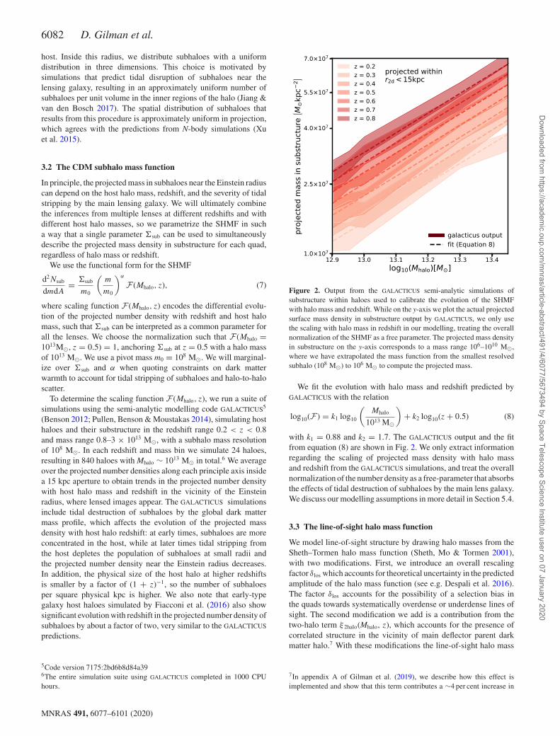
(Benson 2012; Pullen, Benson & Moustakas 2014), simulating hosthaloes and their substructure in the redshift range 0.2 < z < 0.8and mass range 0.8–3 × 10¹³ M�, with a subhalo mass resolutionof 108 M�. In each redshift and mass bin we simulate 24 haloes,resulting in 840 haloes with Mhalo ∼ 1013 M� in total.6 We averageover the projected number densities along each principle axis insidea 15 kpc aperture to obtain trends in the projected number densitywith host halo mass and redshift in the vicinity of the Einsteinradius, where lensed images appear. The GALACTICUS simulationsinclude tidal destruction of subhaloes by the global dark mattermass profile, which affects the evolution of the projected massdensity with host halo redshift: at early times, subhaloes are moreconcentrated in the host, while at later times tidal stripping fromthe host depletes the population of subhaloes at small radii andthe projected number density near the Einstein radius decreases.In addition, the physical size of the host halo at higher redshiftsis smaller by a factor of (1 + z)−1, so the number of subhaloesper square physical kpc is higher. We also note that early-typegalaxy host haloes simulated by Fiacconi et al. (2016) also showsignificant evolution with redshift in the projected number density ofsubhaloes by about a factor of two, very similar to the GALACTICUS
predictions.
5Code version 7175:2bd6b8d84a396The entire simulation suite using GALACTICUS completed in 1000 CPUhours.
Figure 2. Output from the GALACTICUS semi-analytic simulations ofsubstructure within haloes used to calibrate the evolution of the SHMFwith halo mass and redshift. While on the y-axis we plot the actual projectedsurface mass density in substructure output by GALACTICUS, we only usethe scaling with halo mass in redshift in our modelling, treating the overallnormalization of the SHMF as a free parameter. The projected mass densityin substructure on the y-axis corresponds to a mass range 106–1010 M�,where we have extrapolated the mass function from the smallest resolvedsubhalo (108 M�) to 106 M� to compute the projected mass.
We fit the evolution with halo mass and redshift predicted byGALACTICUS with the relation
log10(F ) = k1 log10
(Mhalo
1013 M�
)+ k2 log10(z + 0.5) (8)
with k1 = 0.88 and k2 = 1.7. The GALACTICUS output and the fitfrom equation (8) are shown in Fig. 2. We only extract informationregarding the scaling of projected mass density with halo massand redshift from the GALACTICUS simulations, and treat the overallnormalization of the number density as a free-parameter that absorbsthe effects of tidal destruction of subhaloes by the main lens galaxy.We discuss our modelling assumptions in more detail in Section 5.4.
3.3 The line-of-sight halo mass function
We model line-of-sight structure by drawing halo masses from theSheth–Tormen halo mass function (Sheth, Mo & Tormen 2001),with two modifications. First, we introduce an overall rescalingfactor δlos which accounts for theoretical uncertainty in the predictedamplitude of the halo mass function (see e.g. Despali et al. 2016).The factor δlos accounts for the possibility of a selection bias inthe quads towards systematically overdense or underdense lines ofsight. The second modification we add is a contribution from thetwo-halo term ξ 2halo(Mhalo, z), which accounts for the presence ofcorrelated structure in the vicinity of main deflector parent darkmatter halo.7 With these modifications the line-of-sight halo mass
7In appendix A of Gilman et al. (2019), we describe how this effect isimplemented and show that this term contributes a ∼4 per cent increase in
MNRAS 491, 6077–6101 (2020)
Dow
nloaded from https://academ
ic.oup.com/m
nras/article-abstract/491/4/6077/5673494 by Space Telescope Science Institute user on 07 January 2020

Strong lensing constraints on dark matter 6083
function takes the form
d2Nlos
dmdV= δlos(1 + ξ2halo(Mhalo, z))
d2N
dmdV
∣∣ShethTormen
. (9)
Haloes along the line of sight are rendered in a double-conegeometry with opening angle 3REin, where REin is the Einsteinradius of the main deflector, and a closing angle behind the maindeflector such that the cone closes at the source redshift. Finally,we add negative convergence sheets to subtract the mean expectedconvergence from line-of-sight haloes at each line of sight plane.Without this numerical procedure, lines of sight are systematicallyoverdense relative to the expected matter density of the Universe,akin to lensing in a universe with positive curvature (Birrer et al.2017a). This may bias results as the macromodel will attempt tocompensate for the artificial focusing of light rays in this scenario.
3.4 Modelling free-streaming effects in WDM
Free-streaming refers to the diffusion of dark matter particles outof small peaks in the matter density field in the early Universe. Thishas the effect of erasing structure on scales below a characteristicfree-streaming length which depends on the velocity distribution ofthe dark matter particles, and hence on their mass and formationmechanism. For a more in-depth discussion, see Schneider et al.(2013).
It is convenient to express free-streaming effects in terms of thehalf-mode mass mhm, which is defined in terms of the length-scalewhere the transfer function between the CDM and WDM powerspectra drops to one-half. In the specific case that all of the darkmatter exists in the form of thermal relics, a one-to-one mappingbetween the half-mode mass and the mass of the candidate particlemDM exists, and has the scaling mhm ∝ m−3.33
DM (Schneider et al.2012)
mhm(mDM) = 3 × 10⁸( mDM
3.3 keV
)−3.33M�. (10)
We have run GALACTICUS models (Benson et al. 2013) withWDM mass functions corresponding to 3.3 and 5 keV thermalrelics to investigate the effects of free-streaming on the trends withhost halo mass and redshift of the projected mass in substructurenear the Einstein radius, and determine that the fit in equation (8) iscommon to both CDM and WDM. We therefore use the same scalingfunction F (Mhalo, z) for WDM SHMFs, and model the effects offree-streaming using the fitting formula from Lovell et al. (2014)
dNWDM
dm= dNCDM
dm
(1 + mhm
m
)−1.3. (11)
Since the parameter mhm is related to the WDM transfer function,it should affect the subhalo and field halo mass functions in asimilar manner. We therefore apply the same suppression factorin equation (11) to both the SHMF and the line-of-sight halo massfunction in equations (7) and (9), respectively. Lacking a theoreticalprediction for the evolution of the turnover with redshift, we do notevolve the shape or position of the free-streaming cut-off in themass function at higher redshifts.
In WDM scenarios, the delayed onset of structure formationaffects the assembly history of dark matter haloes and suppressestheir concentrations c ≡ rvir
rs
8 on mass scales that extend above mhm
the frequency of flux ratio perturbations induced by objects outside the virialradius of the main deflector.8We define rvir with respect to the matter density contrast 200ρcrit.
Figure 3. Top: The SHMF as a function of halo mass, redshift, and the half-mode mass mhm = 107 M� with �sub = 0.012 kpc−2. The line-of-sight halomass function looks similar, but evolves differently with redshift. Bottom:The mass–concentration relation for CDM and the same WDM model withmhm = 107 M�. Free-streaming affects the concentration of haloes over oneorder of magnitude above mhm.
(Schneider et al. 2012; Bose et al. 2016). We use the functional formproposed by Bose et al. (2016), and write the WDM concentration–mass relation as
cWDM(m, z)
cCDM(m, z)= (1 + z)β(z)
(1 + 60
mhm
m
)−0.17(12)
with β(z) = 0.026z − 0.04, using the CDM mass–concentrationmodel of Diemer & Joyce (2019) and a scatter of 0.1 dex (Dut-ton & Maccio 2014). The WDM suppression factor for the mass–concentration relation we use was calibrated for haloes on massscales below M200 ∼ 109 M�, and is accurate in the redshift rangez = 0–3. We note that since flux ratios are particularly sensitiveto the central density of perturbing haloes, the suppression ofhalo concentrations far above mhm (because of the factor of 60in equation 12) is possibly the dominant effect of dark matter free-streaming on lensing observables. We plot the SHMF and the halomass–concentration–redshift relation in Fig. 3.
MNRAS 491, 6077–6101 (2020)
Dow
nloaded from https://academ
ic.oup.com/m
nras/article-abstract/491/4/6077/5673494 by Space Telescope Science Institute user on 07 January 2020

6084 D. Gilman et al.
4 TH E DATA
We apply the forward-modelling methodology outlined in Section 2using the physical model described in Section 3 to eight quadruplyimaged quasars. In this section, we describe the sample selection,and how the data for these eight systems were obtained. In Table C1in Appendix C, we summarize the data used in the analysis andprovide the relevant references.
4.1 The narrow-line systems
The quads in our sample have image fluxes measured using thenarrow-line emission from the background quasar. Six of these(WGD 2038, WFI 2033, RX J0911, PS J1606, WGD J0405, andWFI 2026) have flux and astrometry presented by Nierenberg et al.(2019), while the data for B1422 and HE0435 are taken from Nieren-berg et al. (2014) and Nierenberg et al. (2017), respectively. Theflux uncertainties for the narrow-line lenses are estimated from theforward-modelling method used to fit the narrow-line spectra. Foradditional details regarding the measurement methodology for thenarrow-line flux ratios, we refer to Nierenberg et al. (2017, 2019).
Shajib et al. (2019) analysed several systems in our sample. Theymeasured satellite galaxy location and provided the photometricinformation for the systems J1606 and WGD J0405, which we usedto obtain photometric redshifts (see Appendix B).
4.2 Lenses omitted from our sample
We apply our analysis to a sample of eight quads, although addi-tional systems exist in the literature with measured flux ratios. Wechoose only a subset of the total number of possible lenses since theremaining systems either do not have reliable flux measurements, orhave complicated deflector morphology that introduces significantuncertainties in the lens modelling. We do not include lenses withfluxes measured using radio emission from the background quasar.Some of these systems may be analysed in a future work uponrevision of our modelling strategy and new flux measurements.
Specifically, we do not include quads with main lensing galaxiesthat contain stellar discs, since accurate lens models for thesesystems require explicit modelling of the disc. This excludes thesystem J1330 presented by Nierenberg et al. (2019). We also excludeHS 0810, a system with narrow-line flux measurements presented byNierenberg et al. (2019), because the flux from the merging imagesbecomes blended together for source sizes larger than 20 pc. Thiscomplicates our analysis, as our method for computing image fluxeswith extended background sources cannot be applied to mergingpairs when the images blur together.
5 PH Y S I C A L A S S U M P T I O N S A N D P R I O R S
The parametrizations we introduce in Section 3 and the priors usein the forward model reflect certain physical assumptions. In thissection, we describe these assumptions, and the prior probabilitiesattached to each parameter in the forward model for our sample ofquads.
5.1 The extended background source
The effect of a dark matter halo of a given mass on the magnificationof a lensed image is a function of the background source size(Dobler & Keeton 2006), see also fig. 14 in Amara et al. (2006)and fig. 8 in Xu et al. (2012). In general, more extended background
sources are less sensitive to dark matter haloes (in terms of theimage magnifications) on the mass scales relevant for substructurelensing, and the minimum sensitivity threshold for a halo of a givenmax to produce a measurable flux perturbation is determined by thebackground source size.
The lenses in our sample have fluxes measured using emissionfrom the narrow-line region of the background quasar (Nierenberget al. 2017, 2019). The narrow-line region is expected to subtendangular scales larger than a micro-arcsecond, corresponding tophysical scales larger than ∼1 pc, such that it is immune tomicrolensing by stars. This physical extent also corresponds toa light-crossing time greater than the typical time delay betweenlensed images, such that variability in the background quasar shouldbe washed out of the light curves if the source size is indeed largeenough to avoid microlensing.
The size of the narrow-line region typically spans up to ∼60 pc(Muller-Sanchez et al. 2011) defined as the full width at half-maximum (FWHM) of the radially averaged luminosity profile.Upper limits of 50–60 pc may also be obtained by forward modellingthe spectrum of the lensed images themselves (Nierenberg et al.2017). We therefore model the background source as a circularGaussian and impose a uniform prior on the FWHM between25 and −60 pc.
5.2 Halo and subhalo mass ranges
We render haloes for both the line of sight and SHMFs in the range106–1010 M�. Haloes with masses below 106 M� do not leaveimprints on lensing observables for the extended source sizes weconsider, which we verify by comparing distributions of image fluxratios with different minimum subhalo masses. The smallest halomasses flux ratios are sensitive to depend on the background sourcesize and the concentration of the halo, but we estimate through ray-tracing simulations that the lower limit lies somewhere between106 and 107 M� for the smallest source sizes we model. We includethe rare objects more massive than 1010 M� by explicitly includingthem in the lens model, assuming that they host a luminous galaxy,in which case they are detected in the observations of the lensesthemselves. This assumption is consistent with current abundancematching techniques (Kim et al. 2018; Nadler et al. 2019).
5.3 The line-of-sight halo mass function
We use the Sheth–Tormen (Sheth et al. 2001) halo mass functionto model structure along the line of sight, with two modifications:First, we introduce a rescaling term δlos to account for a systematicshift in the predicted mean amplitude of the mass function. Second,we include a term ξ 2halo(Mhalo, z) that rescales the amplitude of themass function near the main deflector to account for the presence ofcorrelated structure in the density field near the parent dark matterhalo. This results in a 5−10 per cent increase in the number haloesnear the main deflector.
Apart from uncertainty in the overall amplitude δlos, we assumethe halo mass function in the lens cone volume is well described bythe mean halo mass function in the Universe. This is a reasonableapproximation as lensing volumes span several Gpc, and we expectfluctuations in the dark matter density along the line of sight shouldaverage out over large distances. We note, however, that there issome scatter among the predictions from different parametrizationsof the halo mass function below 1010 M� (e.g. Despali et al. 2016)and cosmological model uncertainties, for instance associated withσ 8 and �m. It is also possible that lenses are selected preferentially
MNRAS 491, 6077–6101 (2020)
Dow
nloaded from https://academ
ic.oup.com/m
nras/article-abstract/491/4/6077/5673494 by Space Telescope Science Institute user on 07 January 2020

Strong lensing constraints on dark matter 6085
in overdense or underdense lines of sight. We use a flat prior on δlos
between 0.8 and 1.2 to account for these uncertainties.
5.4 The subhalo mass function
Our parametrization of the SHMF is an improvement over previousmodelling efforts in predicting strong lensing observables since itexplicitly accounts for the evolution of the SHMF with redshiftand halo mass, and accounts for the tidal stripping of subhaloes bythe host dark matter halo. However, since the GALACTICUS runsdo not include a central galaxy,9 we cannot predict the effectsof tidal stripping on the projected mass in substructure near theEinstein radius, or the possible redshift and halo mass dependenceof this effect. Since tidal destruction of substructures appears tobe independent of subhalo mass (Garrison-Kimmel et al. 2017;Graus et al. 2018), we absorb the effects of tidal stripping into thenormalization parameter �sub in equation (7). Finally, we note thatthe prescription for rendering haloes outlined in Section 3 does notcouple parameters such as the truncation radius to the concentrationof subhaloes at infall, and does not model the tidal evolution ofsubhaloes from the time of infall until the time of lensing. Theseadditional degrees of modelling complexity will be implemented ina future analysis that uses a larger sample size of lenses.
To determine reasonable bounds on �sub, we compare thepredicted surface density in substructure obtained by integratingequation (7) over mass with the output from N-body simulations,and from the GALACTICUS runs. At z ∼ 0.7, the ∼1013 M� haloes inFiacconi et al. (2016) have projected substructure mass densities of107 M� kpc−2 at 0.02Rvir. Fiacconi et al. (2016) show that this valueincreases when accounting for baryonic contraction of the halo. TheGALACTICUS haloes contain more substructure at the same redshiftwithout accounting for baryonic contraction, corresponding toprojected mass densities between 2.5 × 10⁷ and 6 × 10⁷ M� kpc−2.Both of these projected mass densities would likely decrease whenaccounting for tidal stripping. We note, however, that recent workscall attention to possible numerical issues that can lead to theartificial fragmentation of subhaloes in N-body simulations (vanden Bosch et al. 2018; Errani & Penarrubia 2019). For reference,�sub = 0.012 kpc−2 corresponds to a projected mass density of107 M� kpc−2 at z = 0.5 in a 1013 M� halo, using equation (7).
With these considerations in mind, we use a wide, flat prior on�sub between 0 and 0.1 kpc−2 that should encompass the theoreticaluncertainties present in the literature. We reiterate that by factoringout the evolution with halo mass and redshift, we intend for theparameter �sub to be common for all the lenses in our samplewith scatter from different tidal stripping scenarios and halo-to-halo variance.
The power-law slope α of the SHMF predicted by N-bodysimulations is consistently in the range −1.95 to −1.85 (Springelet al. 2008; Fiacconi et al. 2016), and because tidal strippingappears independent of mass the presence of a central galaxy shouldnot cause significant deviations from this prediction. We thereforeimpose a flat prior on α between −1.95 and −1.85.
5.5 Free-streaming in WDM
The prior on mhm needs to be chosen with care since statementsusing confidence intervals depend on the choice of prior. We specify
9GALACTICUS is capable of including the tidal stripping effects from a centralgalaxy, but we did not include them to minimize computation costs.
the lower bound on the prior for mhm with the WDM mass–concentration relation (equation 12) in mind, since the factor of60 in the denominator of equation (12) results in suppressed haloconcentrations nearly two orders of magnitude above the locationof the turnover in the mass function (see Fig. 3). We choose alower bound for mhm at 104.8 M� that preserves the CDM-predictedhalo concentrations down to 107 M�. At 106 M�, even the coldestmass function we model with mhm = 104.8 M� result in haloconcentrations for 106 M� objects 25 per cent lower than the CDMprediction, but we expect the signal from these very low-mass haloeswill be sub-dominant given that we model extended backgroundsources which decrease sensitivity to low-mass haloes.
5.6 The parent dark matter halo mass
We use information about the mean population of early-type galaxylenses, as well as empirical relations between stellar mass, halomass, and observable quantities such as the image separations andlens/source redshifts, to construct priors for the halo mass of eachsystem.
First, we estimate the ‘lensing’ velocity dispersion from theEinstein radius and lens/source redshifts using the empirical relationbetween the stellar mass and velocity dispersion derived by Augeret al. (2010) for a sample of strong lens galaxies. We account for thescatter between spectroscopic velocity dispersion and the ‘lensing’velocity dispersion (Treu et al. 2006), and uncertainties in the fit byAuger et al. (2010), and convert the estimated stellar mass into ahalo mass using the halo-to-stellar mass ratio Mhalo
M∗ = 75+36−27 inferred
by Lagattuta et al. (2010). The typical uncertainty in the resultingprior for the halo mass is 0.3 dex.
We use this procedure to construct a prior for the halo mass of eachquad, with the exceptions of B1422, PS J1606, and WGD J0405.The stellar velocity dispersions implied by the Einstein radii of thesesystems is significantly lower than the stellar velocity dispersion inthe sample of quads used to calibrate the halo-to-stellar mass ratioin Lagattuta et al. (2010), and as such the estimate of the halomass using the above procedure may not be accurate for thesesystems. For B1422, PS J1606, and WGD J0405, we thereforeassume the population mean of 1013.3 ± 0.3 M� inferred by Lagattutaet al. (2010). We also assume the population mean halo mass forWFI 2026 since the lens redshift used to estimate the central velocitydispersion is very uncertain.
The system RX J0911 is known to reside near a cluster of galaxies,and thus convergence from the cluster halo contributes to the masswithin the Einstein radius. We approximate the contribution fromthe cluster convergence by noting that it should be approximatelyequal to the mean external shear we infer of 0.3. We then rescalethe Einstein radius by
√0.7, since the stellar mass scales as R2
Einand where we have used the fact that the mean convergence insidethe Einstein radius is approximately equal to one for an isothermaldeflector. The priors for the parent halo mass used for each quad arelisted in Table 2.
Since we explicitly model the evolution with halo mass, we vary�sub and Mhalo independently. We note however that Mhalo and �sub
are not completely degenerate in our analysis. While the numberof lens plane subhaloes depends on both parameters, the truncationradius of the subhaloes depends on Mhalo through the distribution ofsubhalo z-coordinates, which in turn depends on the virial radius ofthe parent halo (see equation 6), and the two-halo term appearingin equation (9) depends on the halo mass as a larger halo willhave more correlated structure around it. Fig. 4 provides a visualrepresentation of the link between Mhalo, �sub, α, δlos, and mhm.
MNRAS 491, 6077–6101 (2020)
Dow
nloaded from https://academ
ic.oup.com/m
nras/article-abstract/491/4/6077/5673494 by Space Telescope Science Institute user on 07 January 2020

6086 D. Gilman et al.
Table 2. A summary of deflector zd and source zs redshifts, and satellite galaxies included in the lens model for the quads in our sample. Galaxy positionsprior marked by ∗ denote observed locations, which may differ from the true physical location due to foreground lensing effects from the lens macromodel.We correct for foreground lensing effects in our inference pipeline (see Section 5.8). Satellite galaxy locations are quoted with respect to the light centroid ofthe main deflector (see Table C1). All priors on the satellite mass G2θE
are positive definite. The raised and lowered numbers around the deflector redshifts forPS J1606, WGD J0405, and WFI 2026 are the 68 per cent confidence intervals on the estimated lens redshifts (see Appendix B), which we marginalize over.
Lens zd zs log10Mhalo γ ext G2x G2y G2z G2θE
WGD J0405–3308 0.290.320.25 1.71 N (13.3, 0.3) U (0.02, 0.1) – – – –
HE0435–1223 0.45 1.69 N (13.2, 0.3) U (0.02, 0.13) ∗N (2.585, 0.05)∗ ∗N (−3.637, 0.05)∗ zd + 0.33 N (0.37, 0.03)RX J0911+0551 0.77 2.76 N (13.1, 0.3) see Section 5.9 N (−0.767, 0.05) N (0.657, 0.05) zd N (0.2, 0.2)B1422+231 0.36 3.67 N (13.3, 0.3) U (0.12, 0.35) – – – –PS J1606–2333 0.310.36
0.26 1.70 N (13.3, 0.3) U (0.1, 0.28) N (−0.307, 0.05) N (−1.153, 0.05) zd N (0.27, 0.05)
WFI 2026–4536 1.041.120.9 2.2 N (13.3, 0.3) U (0.03, 0.16) – – – –
WFI 2033–4723 0.66 1.66 N (13.4, 0.3) U (0.13, 0.32) N (0.245, 0.025) N (2.037, 0.025) zd N (0.02, 0.005)∗N (−3.965, 0.025)∗ ∗N (−0.025, 0.025)∗ zd + 0.085 N (0.93, 0.05)
WGD 2038–4008 0.23 0.78 N (13.4, 0.3) U (0.04, 0.12) – – – –
Figure 4. A graphical representation of the dark matter parameters in qs: α, the logarithmic slope of the SHMF, �sub, the overall scaling of the SHMF, mhm, theWDM half-mode mass, δlos, the overall factor for the line-of-sight halo mass function, and Mhalo, the main deflector’s parent halo mass. ξ2halo is implemented
through equation (9) (see Section 3.3). These parameters are linked to the physical dark matter quantities they affect. From left to right: the SHMF d2NdmdA
, the
normalization ρs, scale radius rs, and truncation radius rt of individual haloes (see equation 5), and the line-of-sight halo mass function d2NdmdV
. The priors foreach of these parameters are summarized in Table 2, and discussed at length in Section 5.
5.7 The main deflector lens model
The galaxies that dominate the lensing cross-section are typi-cally massive early-types with stellar velocity dispersions σ >
200 km sec−1 (Gavazzi et al. 2007; Auger et al. 2010; Lagattuta et al.2010). The mass profiles of these systems are typically inferred tobe isothermal, or close to isothermal (Treu et al. 2006, 2009; Augeret al. 2010; Shankar et al. 2017). These observations motivatea simple parametrization for the main deflector lens model, thesingular isothermal ellipsoid plus external shear. We generalize thismodel to a power-law ellipsoid with a variable logarithmic slopeγ macro to account for uncertainties associated with the mass profile ofthe lensing galaxy, and the model-predicted flux ratios. We assume
a flat prior on the power-law slope γ macro between 1.95 and 2.2 foreach deflector (Auger et al. 2010).
In addition to the logarithmic slope of the main deflector massprofile, we sample values for the external shear strength γ ext. Theprior for γ ext is chosen on a lens-by-lens basis by first samplingthe macromodel parameter space without subhaloes to determinea reasonable starting range for γ ext. The width and centre of theprior is adjusted after adding substructure such that the posteriordistribution of γ ext obtained for each lens is contained well withinthe bounds of the prior. The specific priors used for each systemare summarized in Table 2. Finally, we use a Gaussian prior forthe mass centroid of each quad centred on the main deflector light
MNRAS 491, 6077–6101 (2020)
Dow
nloaded from https://academ
ic.oup.com/m
nras/article-abstract/491/4/6077/5673494 by Space Telescope Science Institute user on 07 January 2020

Strong lensing constraints on dark matter 6087
with a variance of 0.05 arcsec, a typical modelling uncertaintyfor quadruple-image systems (Nierenberg et al. 2019; Shajibet al. 2019).
Several studies (Evans & Witt 2003; Hsueh et al. 2016, 2017,2018; Gilman et al. 2017) explore the role of complicated maindeflector morphologies on the model predicted flux ratios. As imagemagnifications are local probes of the gravitational potential, if thereare fluctuations in the surface mass profile on scales comparableto the image separation these structures can affect the imagemagnifications. In particular, stellar discs, if they go unnoticed,can result in systematically inaccurate lens models. With deepHubble Space Telescope (HST) images of the narrow-line quadsin our sample, we can confirm that they do not contain discs, andindeed are representative of the massive elliptical galaxies withroughly isothermal mass profiles that typically act as strong lenses(Auger et al. 2010; Shankar et al. 2017). Gilman et al. (2017)and Hsueh et al. (2018) quantified the systematic uncertaintiesintroduced by modelling early-type galaxy lenses as isothermalellipsoids with fixed logarithmic slopes γ = 2. These works foundthat the resulting systematic uncertainties on image magnificationsare typically less than 10 per cent. This degree of uncertainty iscomparable to the variance in model-predicted image magnifi-cations resulting from marginalizing over a power-law ellipsoidmass model with additional degrees of freedom implementedthrough a variable logarithmic slope γ (Nierenberg et al. 2019).Based on these considerations, we use a power-law ellipsoid withvariable logarithmic slopes γ to model the main deflector massprofile.
Three quads in our sample do not have measured spectroscopicredshifts. For two of these, we use photometry from Shajib et al.(2019) to compute photometric redshifts probability distributionswith the software EAZY (Brammer, van Dokkum & Coppi 2008),and sample the deflector redshift from these distributions in theforward model. For the third system (WFI 2026), which doesnot have multiband photometry from Shajib et al. (2019), weassume a typical velocity dispersion for a massive elliptical galaxy,and derive a probability distribution for the lens redshift frommeasured quantities such as the source redshift and measuredimage separation. We give more details regarding this procedurein Appendix B.
5.8 Satellite galaxies and nearby deflectors
We model satellite galaxies and other deflectors near the mainlens as Singular Isothermal Spheres, and assume they lie at thelens redshift unless they have measured redshifts that place themelsewhere. We marginalize over the position and Einstein radius ofthese objects using Gaussian priors on the positions centred on thelight centroid with a variance of 0.05 arcsec. We use a Gaussian prioron the Einstein radius which is estimated from lens model fitting,or in some cases by direct measurements on the central velocitydispersion (e.g. Wong et al. 2017; Rusu et al. 2019).
In the cases of HE0435 and WFI 2033, the nearby galaxy lies at ahigher redshift than the main lens plane. The light from the galaxyis therefore subject to lensing by the main deflector, and its truephysical location differs from its observed position. We estimate thetrue physical locations of these objects by sampling the macromodelparameter space using the image positions as constraints, andread out the physical position of background satellite given itsobserved (lensed) position. We then place the satellite at this derivedphysical location in the forward model sampling with uncertaintiesof 0.05 arcsec. This process significantly speeds up the lensing
computations since it does not require the continuous re-evaluationof the physical satellite location given its observed position duringeach lens model computation.10 The boost in speed comes at thecost of decoupling the satellite galaxy position from the dark matterparameters qs in the inference, but we expect the covariance betweenthese quantities will be negligible because the satellite galaxies, evenwhen their locations are corrected for foreground lensing effects,are relatively far from the images, introducing convergence at themain deflector light centroid of <0.1 in both cases.11
In the case of HE0435, we estimate the angular location withoutforeground lensing of the satellite to be (−2.37, 2.08), whilefor WFI 2033 we obtain (−3.63, −0.08), for observed (lensed)locations of (−2.911, 2.339) and (−3.965, −0.022), respectively.These coordinates are with respect to the galaxy light centroid (seeTable C1). The angular locations of the lensed background satellitesare closer to the mass centroid of the main deflector, just as thephysical location of the lensed background quasar is concentricwith the mass centroid.
The lens-specific priors on satellite galaxies are summarized inTable 2.
5.9 Lens-specific modelling for RX J0911+0551 and WGD2038–4008
For system RX J0911, we alter the modelling strategy slightly toincrease computational efficiency by allowing the external shearstrength γ ext to vary freely while solving for macromodel parame-ters that fit the observed image positions. For the system WGD 2038,we widen the prior on the power-law slope of the macromodel asthe posterior using the default range for γ macro between 1.95 and2.2 is biased towards higher values of γ macro. For WGD 2038, theposterior peaks at γ macro ∼ 2.25.
6 R ESULTS
In this section, we present the results of our analysis. We begin inSection 6.1 by showing dark matter halo convergence maps for someof the top-ranked realizations drawn in the forward model. We thendisplay the posterior distributions for a few individual lenses, show-ing the simultaneous inference of parameters describing the macrolens model and the dark matter hyper-parameters. In Section 6.2,we present the constraints on the abundance of substructure anddark matter warmth for the full sample of 11 quads.
6.1 Top-ranked realizations and posteriors for individuallenses
Minimizing the summary statistic in equation (4) selects realizationsthat resemble the observed data as closely as possible. Thisguarantees that the set of accepted dark matter hyper-parameters
10The physical location of the nearby galaxy needs to be continuously re-evaluated because it’s observed location depends on the foreground lensingeffects from the macromodel, and the parameters describing the macromodelare continuously changing while finding a solution to the lens equation(equation 3).11The default convention in LENSTRONOMY is to place deflectors at theirobserved angular locations in the Universe, but it is now possible (in codeversions 0.8.0 +) to specify which objects should be treated using theobserved (lensed) position instead. We note that the default convention inLENSMODEL (Keeton, Kochanek & Seljak 1997) is to place objects at theirobserved (lensed) locations during multiplane ray-tracing.
MNRAS 491, 6077–6101 (2020)
Dow
nloaded from https://academ
ic.oup.com/m
nras/article-abstract/491/4/6077/5673494 by Space Telescope Science Institute user on 07 January 2020
6088 D. Gilman et al.
qs yield an accurate approximation of the true posterior distributionfor each individual lens with data dn: p(qs|dn). For visualizationpurposes, and to reinforce the fact that the top-ranked realizationslook like the data and satisfy Slens ≈ 0 (equation 4), in Fig. 5 wedisplay the dark matter halo effective multiplane convergence mapsfor some of the top-ranked realizations for a subset of quads in oursample. The effective multiplane convergence is defined as half thedivergence of the full deflection field α
κeffective ≡ 1
2∇ · α. (13)
This definition of the multiplane convergence accounts for the non-linear effects present in multiplane lensing, and satisfies the single-plane definition of convergence as second derivatives of a lensingpotential in the absence of multiple lens planes.
To visualize individual realizations of dark matter structure,we define κeffective(halo) ≡ κeffective − κmacro, where κmacro is theconvergence from the lens macromodel, including satellite galaxiesand nearby deflectors. In the resulting convergence maps, haloeslocated behind the main lens plane appear sheared tangentiallyaround the Einstein radius due to coupling to the large deflectionsproduced by the macromodel.
In Fig. 5, we show κeffective(halo) maps of randomly selected real-izations of dark matter structure whose corresponding qs parameterswere accepted in the final posterior on the basis of their summarystatistic Slens. The specific realizations and the corresponding darkmatter parameters qs correspond to a diverse set of substructurepopulations, warm and cold, which yield similarly good fits to theobserved flux ratios satisfying Slens ∼ 0. Some models, however, pre-dict flux ratios that match the observed flux ratios more frequentlythan others. In terms of the Approximate Bayesian Computingalgorithm described in Section 2, the frequency with which one darkmatter model relative to another predicts observables that resemblethe data is a surrogate for the relative likelihood of the models.The probability of accepting a proposed qs based on the summarystatistic in equation (4) is therefore equal to the likelihood p(dn|qs)(equation 2), even though the form of this function is unknown andit is never directly evaluated.
The top-ranked realizations for B1422 shown in Fig. 5 eachhave a relatively massive dark matter halo, or several smaller ones,located near the top left merging triplet image with (normalized)flux 0.88. This is in agreement with the analysis by Nierenberg et al.(2014), who find that a blob of dark matter near this image bringsthe model-predicted flux ratios into agreement with a smooth lensmodel.
Although not obvious from examining Fig. 5, the underlyingmacromodels for each accepted realization are unique, with dif-ferent external shears, power-law slopes, lens ellipticity, etc. Wemarginalize over different macromodel configurations by simulta-neously sampling the macromodel parameters and the dark matterhyper-parameters in the forward model. To illustrate, in Figs 6, 7,and 8 we show the posterior distributions for several parameters inthe lens macromodel, along with the dark matter hyper-parameters�sub and mhm for HE0435, WFI 2033, and RX J0911. The systemHE0435 generally favours models with low SHMF normalizations(low �sub), or a turnover in the mass function with higher �sub. Thesystem WFI 2033 is the opposite, with a posterior favouring CDM-like mass functions with many lens plane subhaloes. The systemRX J0911 lies somewhere in between, with a peak in the posteriordistribution of mhm near 107 M�.
For each of these systems, in particular WFI 2033, there is avisibly obvious covariance between the overall normalization of
the main deflector mass profile bmacro,12 and the parameters �sub
and mhm. This covariance is readily understood: To reproduce theobserved image positions, the macromodel responds to the additionof mass in the form of subhaloes in main lens plane by decreasingthe overall normalization of the main deflector mass profile, andhence these quantities are anticorrelated. Similarly, WDM modelscorrespond to macromodels with larger bmacro because WDMrealizations contain fewer subhaloes. Interestingly, there is somestructure in the posterior distribution for the lens ellipticity ε inWFI 2033, and both mhm and �sub.
By simultaneously sampling the lens macromodel and darkmatter hyper-parameters, we obtain posterior distributions thataccount for covariance between M and qs. We do not use lensmodel priors from more sophisticated lens modelling efforts (e.g.Wong et al. 2017; Shajib et al. 2019) because these analyses didnot include substructure in the lens models and therefore do notaccount for covariances between the macromodel parameters andthe dark matter parameters of interest. For the same reason, we donot decouple the lens macromodel parameters from the dark matterhyper-parameters by first sampling the macromodel parameterspace that fits the image positions, and using these distributionsas priors in the forward modelling.
6.2 Constraints on the free-streaming length of dark matter
For each quad, we obtain a joint likelihood between the macro-model parameters M and the dark matter-hyper parameters qs. Wemarginalize over the parameters in this 20+dimensional space toobtain the four-dimensional space of qs parameters that includeslogarithmic slope of the SHMF α, the scaling of the line-of-sighthalo mass function δlos, the overall scaling of the SHMF �sub, andthe half-mode mass mhm. We reiterate that these four parametersdescribe universal properties of dark matter and should thereforebe common to all the lenses, while the parameters M and the halomass Mhalo are lens-specific. After marginalizing, we compute theproduct of the resulting likelihoods and obtain the desired posteriordistribution in equation (1), which we display in Fig. 9.
The marginalized constraints on mhm rule out mhm > 107.8 M� at2σ , corresponding to thermal relic particle mass of < 5.2 keV. It isapparent from Fig. 9 that mhm and �sub are correlated, since haloesadded by increasing the normalization can be subsequently removedby increasing mhm such that the total amount of lensing substructureremains relatively constant. As a result, the marginalized distribu-tion for the normalization �sub appears unconstrained from above,as the normalization can be significantly higher in WDM scenarios.With only eight quads we cannot simultaneously measure mhm and�sub, although our previous forecasts indicate this is possible withmore lenses (Gilman et al. 2018).
The constraints on dark matter warmth in terms of confidenceintervals depend on the range of allowed values specified by theprior on �sub. Similarly, the confidence interval on mhm dependson the lower bound of this parameter that is set by the prior onmhm. As discussed in Section 5.5, we have chosen the prior on mhm
to encompass the region of parameter space where the data canconstrain mhm, keeping in mind that the WDM mass–concentrationrelation affects the central densities of subhaloes 60 times abovemhm (equation 12), and the upper bound of �sub = 0.1 kpc−2
is a conservative choice as most N-body simulations and the
12bmacro has units of convergence, or projected mass density divided by thecritical surface mass density for lensing.
MNRAS 491, 6077–6101 (2020)
Dow
nloaded from https://academ
ic.oup.com/m
nras/article-abstract/491/4/6077/5673494 by Space Telescope Science Institute user on 07 January 2020

Strong lensing constraints on dark matter 6089
Figure 5. Dark matter halo effective multiplane convergence maps for some of the highest ranked realizations for the subset of quads B1422, WGD J0405,WFI 2033, and RX J0911, each of which has flux ratios inconsistent with smooth lens models. The definition of the effective multiplane convergence takes intoaccount the non-linear effects present in multiplane lensing, and is defined with respect to the mean dark matter density in the Universe such that some regionsare underdense (blue), while other regions (specifically, dark matter haloes) are overdense (red). The SHMF normalization, line-of-sight normalization, halomass and half-mode mass are displayed for each realization. The green text/circles denote observed image positions and fluxes, while the black text/crossesdenote the model positions and fluxes. The forward-model data sets fit the image positions and fluxes to within the measurement uncertainties.
MNRAS 491, 6077–6101 (2020)
Dow
nloaded from https://academ
ic.oup.com/m
nras/article-abstract/491/4/6077/5673494 by Space Telescope Science Institute user on 07 January 2020

6090 D. Gilman et al.
Figure 6. Joint posterior distribution for a subset of M and qs parameters for the system HE0435. We display the normalization of the main deflector lens modelbmacro, the external shear strength and position angle γ ext and θ ext, the deflector ellipticity ε, the power-law slope of the main deflector mass profile γ macro, theEinstein radius of the satellite galaxy G2θE
, the normalization of the SHMF �sub, and the half-mode mass mhm. We simultaneously sample the distributions ofthese parameters to account for covariance between the macromodel and the dark matter hyper-parameters qs. The vertical lines denote 95 per cent confidenceintervals.
GALACTICUS runs predict values below 0.05 kpc−2. In light of thesecomplications, we also quote likelihood ratios which do not dependon the choice of prior. Relative to the peak of the mhm posterior, weobtain likelihood ratios for WDM with mhm = 108.2 M� (mhm =108.6 M�) of 7:1 (30:1).13
The posterior for δlos indicates the data favour more line-of-sight structure, but the preference is not statistically significant. The
13We remind the reader that the relative heights of the peaks in the posteriorsomewhat depend on the binning method, or in this case the bandwidthestimator of the KDE. In this work, we have applied a KDE with a first-order boundary correction and a bandwidth selected according to Scott’sfactor (Scott 1992).
parameters δlos and �sub are anticorrelated, as one would expect asone can, to a certain degree, remove lens plane subhaloes and replacethem with line-of-sight haloes while keeping the total amount of fluxperturbation constant. This is not a perfect degeneracy, however,since lensing efficiency and the relative number of subhaloes andline-of-sight haloes changes with redshift. Thus, a larger sampleof quads at different redshifts could break the covariance between�sub and δlos.
6.3 Constraints on the subhalo mass function assuming CDM
We perform a suite of CDM simulations using the same priors listedin Table 2, minus the WDM parameter mhm, with the aim of inferring
MNRAS 491, 6077–6101 (2020)
Dow
nloaded from https://academ
ic.oup.com/m
nras/article-abstract/491/4/6077/5673494 by Space Telescope Science Institute user on 07 January 2020

Strong lensing constraints on dark matter 6091
Figure 7. Joint posterior distribution for a subset of M and qs parameters for the system WFI 2033. The parameters are the same as in Fig. 6. In addition tothe main deflector we model two additional nearby galaxies, with Einstein radii G2θE (1) and G2θE (2). We show the distributions of the Einstein radius for thelarger nearby galaxy (G2θE (2)), whose position we correct for foreground lensing effects (see Section 5.8).
�sub. We marginalize over δlos, and over a theoretical-motivatedprior on α (between −1.95 and −1.85) based on predictions fromN-body simulations (Springel et al. 2008; Fiacconi et al. 2016).
The inference on �sub is shown in Fig. 10. We infer �sub =0.055 kpc−2, with a 1σ confidence interval 0.029 < �sub <
0.083 kpc−2. At the 2σ level we obtain �sub > 0.008 kpc−2. Wedo not quote an upper 2σ bound on �sub as it is prior dominated.To put these numbers in physical units, the mean value of �sub
corresponds to a mean projected mass in substructure for the lensesin our sample between 106 and 109 M� of 4.0 × 10⁷ M� kpc−2, andthe 1σ confidence interval corresponds to 2.0−6.1 × 10⁷ M� kpc−2.At 2σ , the projected mass constraint is �sub > 0.6 × 10⁷M�kpc−2.To convert into the average projected mass, we have computed the
average of the projected masses for each of the eight lenses in oursample, using the scaling of the halo mass function with redshift inequation (8) while assuming a halo mass of 1013 M�.
7 D I SCUSSI ON AND C ONCLUSI ONS
In this section, we review the main results of this work and discussthe implications for cold and warm dark matter. In Section 7.1, wesummarize our main results, and in Section 7.2, we compare ourresults with those obtained in previous works. In Section 7.3, wediscuss the sources of systematic uncertainty in our analysis, andwe conclude in Section 7.4 by discussing the implications of ourresult for cold and warm dark matter.
MNRAS 491, 6077–6101 (2020)
Dow
nloaded from https://academ
ic.oup.com/m
nras/article-abstract/491/4/6077/5673494 by Space Telescope Science Institute user on 07 January 2020

6092 D. Gilman et al.
Figure 8. Joint posterior distribution for a subset of M and qs parameters for the system RX J0911. The parameters are the same as in Fig. 6.
7.1 Summary of the analysis and main results
We have carried out a measurement of the free-streaming lengthof dark matter and the SHMF using a sample of eight quadruplyimaged quasars. The methodology we use to constrain the darkmatter parameters of interest has been tested and verified withsimulated data (Gilman et al. 2019). Lenses that show evidence formorphological complexity in the form of stellar discs are excludedfrom our analysis. We model haloes both in the main deflector andalong the line of sight, including correlated structure around themain deflector through the two-halo term, and account for evolutionof the projected SHMF with redshift and halo mass using a suiteof simulations using the semi-analytic modelling code GALACTI-CUS. We compute image flux ratios by ray-tracing to finite-sizebackground sources, which correctly accounts for the sensitivity ofimage flux ratios to perturbing haloes. We also marginalize overthe macromodel parameters for each system, including the power-
law slope of the main deflector, and simultaneously constrain thelens macromodel and dark matter hyper-parameters to account forcovariance between these quantities. In addition to the turnoverin the halo mass function, we model WDM free-streaming effectson the mass–concentration relation, accounting for the effect ofreduced central densities of WDM haloes on lensing observables.
The main results of this analysis are summarized as follows:
(i) We constrain the half-mode mass mhm (thermal relic darkmatter particle mass) to mhm < 107.8 M� (mDM > 5.2 keV) at 2σ .Since the confidence intervals depend on the prior used for bothmhm and �sub, we also quote likelihood ratios relative to the peakof the posterior distribution for mhm: we disfavour mhm = 108.2 M�(mDM = 4 keV) with a likelihood ratio of 7:1, and with mhm =108.6 M� (mDM = 3.0 keV) the relative likelihood is 30:1. Thesebounds are marginalized over the amplitude of the SHMF, the
MNRAS 491, 6077–6101 (2020)
Dow
nloaded from https://academ
ic.oup.com/m
nras/article-abstract/491/4/6077/5673494 by Space Telescope Science Institute user on 07 January 2020

Strong lensing constraints on dark matter 6093
Figure 9. Marginal and joint posterior distributions for the dark matter hyper-parameters δlos, α, �sub, and mhm, which represent the overall scaling of theline-of-sight halo mass function, the logarithmic slope of the SHMF, the global normalization of the SHMF that accounts for evolution with halo mass andredshift (see equation 7), and the half-mode mass mhm relevant to WDM models. The contours show 68 per cent and 95 per cent confidence intervals, while thedot–dashed lines on the marginal distributions show the 95 per cent confidence intervals.
amplitude of the line-of-sight halo mass function, the power-lawslope of the SHMF, the parent halo mass, the background sourcesize, and the parameters describing the main deflector mass profile.
(ii) Assuming CDM, we infer a value of the global amplitude ofthe SHMF�sub = 0.0550.032
−0.027kpc−2 at 1σ , and �sub > 0.008kpc−2
at 2σ . In our lens sample, these values correspond to an averageprojected mass density in substructure between 106 and 109 M� of4.0+2.1
−2.0 × 10⁷M�kpc−2 and a lower bound of 0.6 × 10⁷ M� kpc−2,respectively. At fixed redshifts, for a 1013 M� halo at z = 0.2 (z =0.6) the 1σ constraint corresponds to a projected mass in substruc-ture of 1.9+0.9
−0.9 × 10⁷ M� kpc−2 (4.1+2.0−2.0 × 10⁷ M� kpc−2) in the
subhalo mass range 106–109 M�. The 2σ constraint corresponds toa projected mass in substructure of greater than 0.3 × 10⁷ M� kpc−2
(0.6 × 10⁷ M� kpc−2) in the same mass range.
7.2 Discussion and comparison with previous work
7.2.1 Constraints on dark matter warmth and the amplitude of theCDM subhalo mass function
The first comprehensive analysis of multiply-imaged quasars wascarried out by DK2, who inferred a projected mass fraction in sub-structure fsub
14 in the range 0.006 < fsub < 0.07 at 2σ modelling
14Throughout this section, we will use fsub to refer to the average massfraction in substructure inferred from a sample of multiple lenses in haloesof different masses at different redshifts, and fsub to refer to the mass fractionin substructure implied by a certain �sub value at a specific redshift and halomass.
MNRAS 491, 6077–6101 (2020)
Dow
nloaded from https://academ
ic.oup.com/m
nras/article-abstract/491/4/6077/5673494 by Space Telescope Science Institute user on 07 January 2020

6094 D. Gilman et al.
Figure 10. Inference on the global normalization of the SHMF �sub
assuming CDM, marginalized over the logarithmic slope α and uncertaintyin the overall amplitude of the line-of-sight halo mass function δlos. Theblue dashed lines shows the mean of the marginal distribution, while theblack solid (dashed) lines represent 68 per cent and 95 per cent confidenceintervals. The contours in the joint distribution also represent 68 per cent and95 per cent confidence intervals.
only lens-plane substructure, and assuming CDM. Recently, H19improved on the analysis of DK2 by including the effects of line-of-sight haloes, measuring 0.006 < fsub < 0.018 at 1σ with a meanof 0.011 assuming CDM, and also constrained the free-streaminglength of dark matter to mhm < 108.4 (mDM > 3.8 keV).
The 2σ bound from H19 of mhm < 108.4 M� is weaker than theconstraint from this work mhm < 107.8 M�. One possible reasonfor this difference is that unlike previous work (Birrer et al. 2017b;Gilman et al. 2018, 2019) H19 did not model the suppression of themass–concentration relation in WDM scenarios, which suppressesthe lensing signal more than one order of magnitude above theposition of the turnover in the mass function. This is of particularrelevance for flux ratio studies because the effect of a perturbing darkmatter halo depends on its central density profile. Free-streamingeffects on the mass–concentration relation therefore increase therelative differences between CDM and WDM on the scales relevantfor substructure lensing, which leads to greater constraining powerover WDM models. Finally, we note that in a future analysismodelling the tidal evolution of substructures from the time ofinfall to the time of lensing may introduce additional constrainingpower over WDM models by coupling the structural parameters ofsubhaloes at the time of lensing to their structural properties, suchas concentration, at the time of infall.
To facilitate direct comparison between this analysis and that ofDK2 and H19 regarding the constraints on the SHMF assumingCDM, we convert our �sub values into estimates of fsub bycomputing the projected mass density �, and then using the fact that
��crit
= 0.5 near the Einstein radius, where �crit is the critical surfacemass density for lensing. In these conversions, we also assume a halomass of 1013 M�, and take care to compute fsub using the same massrange 106–109 M� used by H19. Our 2σ bounds on �sub correspondto an average mass fraction in substructure fsub > 0.005 with a
mean of fsub = 0.035. At 1σ 0.018 < fsub < 0.056. This result isstatistically consistent with the constraints from H19, and also withthose of DK2.
There are several key differences between our analysis and thoseof H19 and DK2 that pull in opposite directions in terms of con-straining power over dark matter models. As mentioned previouslywe model free-streaming effects on the mass–concentration relation,and include the contribution from the two-halo term to accountfor correlated structure near the main deflector. These pieces ofadditional physics add information and increase our constrainingpower over WDM models. On the other hand, accounting forfinite-size background sources decreases the expected magnificationsignal caused by dark matter haloes and subhaloes, and we expectto infer a higher normalization of the SHMF in our analysis asmore substructure is needed to produce the same degree of fluxperturbation. Explicitly, by ray-tracing to finite-size backgroundsources we find that the peak of the magnification cross-sectionfor a 5 × 10⁷ M� halo is reduced by a factor of two for a 15 pcbackground source relative to a 5 pc background source, and bya factor of three for a 40 pc source. The simplifying assumptionof point-sources for the background quasar invoked by H19 andDK2 introduces signal from low-mass haloes whose effects wouldotherwise be washed out by an extended source.
The tidal truncation of lens plane subhaloes that we model mayalso reduce the overall impact of subhaloes on lensing observables.We also marginalize over the power-law slope of the main deflectorand simultaneously sample the macromodel parameters and thedark matter hyper-parameters. These processes introduce additionalcovariances in the posterior distributions, and should lead to weakerconstraints on �sub and mhm.
Other lensing studies, primarily those using the technique ofgravitational imaging, have also sought to measure the SHMF.Vegetti et al. (2014) inferred fsub = 0.00640.0080
−0.0042 at 1σ in the massrange 4 × 10⁶–4 × 10⁹ M� assuming a prior on the slope ofthe SHMF centred on α = −1.9, while Hezaveh et al. (2016b)constrained the normalization of SHMF assuming α = −1.9,inferring ffsub values comparable to the median fsub = 0.02 resultfrom DK2 (and our constraint), but with larger uncertainties.
To compare with the analysis of Vegetti et al. (2014), we assumea halo mass of 1013 M� at a lens redshift zd = 0.25 and a sourceat zsrc = 0.7, characteristic values for the lens sample analysed byVegetti et al. (2014). Using these values with our expression forthe SHMF in equation (7), we obtain fsub = 0.014+0.008
−0.007 between4 × 106 and 6 × 10⁹ M� at 1σ , in the same mass range used byVegetti et al. (2014). This result is consistent with that of Vegettiet al. (2014).15 We quote constraints on fsub to make comparisonswith previous work, but we caution that the conclusions derivedfrom inferences of fsub should be interpreted with care. The phys-ical meaning of this parameter depends on specific assumptionsregarding the subhalo mass range and the contribution from darksubstructure to the convergence near the Einstein radius, which maychange with halo mass and redshift.
Comparing our results with semi-analytic simulations of massive1013 M� hosts, our results in terms of the projected mass insubstructure is consistent with the GALACTICUS simulations usedto calibrate the evolution of the SHMF with halo mass and redshift.
15Although Vegetti et al. (2014) did not model line-of-sight haloes, the lowlens/source redshifts of their sample lessen the impact of line-of-sight haloeson the inferred subhalo mass fraction such that we may compare our results,which include line-of-sight haloes, with theirs.
MNRAS 491, 6077–6101 (2020)
Dow
nloaded from https://academ
ic.oup.com/m
nras/article-abstract/491/4/6077/5673494 by Space Telescope Science Institute user on 07 January 2020
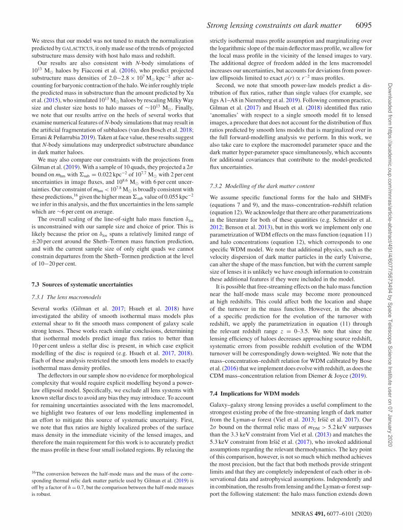
Strong lensing constraints on dark matter 6095
We stress that our model was not tuned to match the normalizationpredicted by GALACTICUS, it only made use of the trends of projectedsubstructure mass density with host halo mass and redshift.
Our results are also consistent with N-body simulations of1013 M� haloes by Fiacconi et al. (2016), who predict projectedsubstructure mass densities of 2.0−2.8 × 10⁷ M� kpc−2 after ac-counting for baryonic contraction of the halo. We infer roughly triplethe predicted mass in substructure than the amount predicted by Xuet al. (2015), who simulated 1013 M� haloes by rescaling Milky Waysize and cluster size hosts to halo masses of ∼1013 M�. Finally,we note that our results arrive on the heels of several works thatexamine numerical features of N-body simulations that may result inthe artificial fragmentation of subhaloes (van den Bosch et al. 2018;Errani & Penarrubia 2019). Taken at face value, these results suggestthat N-body simulations may underpredict substructure abundancein dark matter haloes.
We may also compare our constraints with the projections fromGilman et al. (2019). With a sample of 10 quads, they projected a 2σ
bound on mhm with �sub = 0.022 kpc−2 of 107.7 M� with 2 per centuncertainties in image fluxes, and 108.6 M� with 6 per cent uncer-tainties. Our constraint of mhm < 107.8 M� is broadly consistent withthese predictions,16 given the higher mean �sub value of 0.055 kpc−2
we infer in this analysis, and the flux uncertainties in the lens samplewhich are ∼6 per cent on average.
The overall scaling of the line-of-sight halo mass function δlos
is unconstrained with our sample size and choice of prior. This islikely because the prior on δlos spans a relatively limited range of±20 per cent around the Sheth–Tormen mass function prediction,and with the current sample size of only eight quads we cannotconstrain departures from the Sheth–Tormen prediction at the levelof 10−20 per cent.
7.3 Sources of systematic uncertainties
7.3.1 The lens macromodels
Several works (Gilman et al. 2017; Hsueh et al. 2018) haveinvestigated the ability of smooth isothermal mass models plusexternal shear to fit the smooth mass component of galaxy scalestrong lenses. These works reach similar conclusions, determiningthat isothermal models predict image flux ratios to better than10 per cent unless a stellar disc is present, in which case explicitmodelling of the disc is required (e.g. Hsueh et al. 2017, 2018).Each of these analysis restricted the smooth lens models to exactlyisothermal mass density profiles.
The deflectors in our sample show no evidence for morphologicalcomplexity that would require explicit modelling beyond a power-law ellipsoid model. Specifically, we exclude all lens systems withknown stellar discs to avoid any bias they may introduce. To accountfor remaining uncertainties associated with the lens macromodel,we highlight two features of our lens modelling implemented inan effort to mitigate this source of systematic uncertainty. First,we note that flux ratios are highly localized probes of the surfacemass density in the immediate vicinity of the lensed images, andtherefore the main requirement for this work is to accurately predictthe mass profile in these four small isolated regions. By relaxing the
16The conversion between the half-mode mass and the mass of the corre-sponding thermal relic dark matter particle used by Gilman et al. (2019) isoff by a factor of h = 0.7, but the comparison between the half-mode massesis robust.
strictly isothermal mass profile assumption and marginalizing overthe logarithmic slope of the main deflector mass profile, we allow forthe local mass profile in the vicinity of the lensed images to vary.The additional degree of freedom added in the lens macromodelincreases our uncertainties, but accounts for deviations from power-law ellipsoids limited to exact ρ(r) ∝ r−2 mass profiles.
Second, we note that smooth power-law models predict a dis-tribution of flux ratios, rather than single values (for example, seefigs A1–A8 in Nierenberg et al. 2019). Following common practice,Gilman et al. (2017) and Hsueh et al. (2018) identified flux ratio‘anomalies’ with respect to a single smooth model fit to lensedimages, a procedure that does not account for the distribution of fluxratios predicted by smooth lens models that is marginalized over inthe full forward-modelling analysis we perform. In this work, wealso take care to explore the macromodel parameter space and thedark matter hyper-parameter space simultaneously, which accountsfor additional covariances that contribute to the model-predictedflux uncertainties.
7.3.2 Modelling of the dark matter content
We assume specific functional forms for the halo and SHMFs(equations 7 and 9), and the mass–concentration–redshift relation(equation 12). We acknowledge that there are other parametrizationsin the literature for both of these quantities (e.g. Schneider et al.2012; Benson et al. 2013), but in this work we implement only oneparametrization of WDM effects on the mass function (equation 11)and halo concentrations (equation 12), which corresponds to onespecific WDM model. We note that additional physics, such as thevelocity dispersion of dark matter particles in the early Universe,can alter the shape of the mass function, but with the current samplesize of lenses it is unlikely we have enough information to constrainthese additional features if they were included in the model.
It is possible that free-streaming effects on the halo mass functionnear the half-mode mass scale may become more pronouncedat high redshifts. This could affect both the location and shapeof the turnover in the mass function. However, in the absenceof a specific prediction for the evolution of the turnover withredshift, we apply the parametrization in equation (11) throughthe relevant redshift range z = 0–3.5. We note that since thelensing efficiency of haloes decreases approaching source redshift,systematic errors from possible redshift evolution of the WDMturnover will be correspondingly down-weighted. We note that themass–concentration–redshift relation for WDM calibrated by Boseet al. (2016) that we implement does evolve with redshift, as does theCDM mass–concentration relation from Diemer & Joyce (2019).
7.4 Implications for WDM models
Galaxy–galaxy strong lensing provides a useful compliment to thestrongest existing probe of the free-streaming length of dark matterfrom the Lyman-α forest (Viel et al. 2013; Irsic et al. 2017). Our2σ bound on the thermal relic mass of mDM > 5.2 keV surpassesthan the 3.3 keV constraint from Viel et al. (2013) and matches the5.3 keV constraint from Irsic et al. (2017), who invoked additionalassumptions regarding the relevant thermodynamics. The key pointof this comparison, however, is not so much which method achievesthe most precision, but the fact that both methods provide stringentlimits and that they are completely independent of each other in ob-servational data and astrophysical assumptions. Independently andin combination, the results from lensing and the Lyman-α forest sup-port the following statement: the halo mass function extends down
MNRAS 491, 6077–6101 (2020)
Dow
nloaded from https://academ
ic.oup.com/m
nras/article-abstract/491/4/6077/5673494 by Space Telescope Science Institute user on 07 January 2020

6096 D. Gilman et al.
in a scale-free manner to mass scales of ∼108 M�, where haloesare mostly, if not completely, dark. There appears to be little roomleft for a viable WDM solution to the small-scale issues of CDM.
AC K N OW L E D G E M E N T S
We thank the anonymous referee for a careful reading of the paperand thoughtful comments. We are also grateful to Alex Kusenkoand Annika Peter for useful discussions throughout the course ofthis project, and thank David Gilman for useful comments on anearly draft version of this work.
DG, TT, and SB acknowledge support by the US NationalScience Foundation through grant AST-1714953. DG, TT, SB,and AN acknowledge support from HST-GO-15177. AJB andXD acknowledge support from NASA ATP grant 17-ATP17-0120.Support for Program number GO-15177 was provided by NASAthrough a grant from the Space Telescope Science Institute, whichis operated by the Association of Universities for Research in As-tronomy, Incorporated, under NASA contract NAS5-26555. TT andAN acknowledge support from HST-GO-13732. AN acknowledgessupport from the NASA Postdoctoral Program Fellowship, the UCIrvine Chancellor’s Fellowship, and the Center for Cosmology andAstroparticle Physics Fellowship.
This work used computational and storage services associatedwith the Hoffman2 Shared Cluster provided by the UCLA Institutefor Digital Research and Education’s Research Technology Group.This work also used computational and storage services associatedwith the Aurora and Halo super computers. These resources wereprovided by funding from the JPL Office of the Chief InformationOfficer. In addition, calculations were performed on the memexcompute cluster, a resource provided by the Carnegie Institution forScience.
Part of this work is based on observations made with theNASA/ESA Hubble Space Telescope, obtained at the Space Tele-scope Science Institute, which is operated by the Associationof Universities for Research in Astronomy, Inc., under NASAcontract NAS 5-26555. These observations are associated withprograms #13732 and #15177. Support for programs #13732 and#15177 was provided by NASA through a grant from the SpaceTelescope Science Institute, which is operated by the Association ofUniversities for Research in Astronomy, Inc., under NASA contractNAS5-26555.
RE FERENCES
Abazajian K. N., Kusenko A. 2019, Phys. Rev. D, 100, 103513Agnello A. et al., 2018, MNRAS, 479, 4345Akeret J., Refregier A., Amara A., Seehars S., Hasner C., 2015, J. Cosmol.
Astropart. Phys., 8, 043Amara A., Metcalf R. B., Cox T. J., Ostriker J. P., 2006, MNRAS, 367, 1367Anguita T. et al., 2018, MNRAS, 480, 5017Angulo R. E., Hahn O., Ludlow A. D., Bonoli S., 2017, MNRAS, 471, 4687Auger M. W., Treu T., Bolton A. S., Gavazzi R., Koopmans L. V. E., Marshall
P. J., Moustakas L. A., Burles S., 2010, ApJ, 724, 511Avila-Reese V., Colın P., Valenzuela O., D’Onghia E., Firmani C., 2001,
ApJ, 559, 516Bade N., Siebert J., Lopez S., Voges W., Reimers D., 1997, A&A, 317, L13Baltz E. A., Marshall P., Oguri M., 2009, J. Cosmol. Astropart. Phys., 1, 015Bayer D., Chatterjee S., Koopmans L. V. E., Vegetti S., McKean J. P., Treu
T., Fassnacht C. D., 2018, preprint (arXiv:1803.05952)Beaumont M. A., Zhang W., Balding D. J., 2002, Genetics, 162, 2025Benson A. J., 2012, New Astron., 17, 175Benson A. J. et al., 2013, MNRAS, 428, 1774
Birrer S., Amara A., 2018, Phys. Dark Universe, 22, 189Birrer S., Welschen C., Amara A., Refregier A., 2017a, J. Cosmol. Astropart.
Phys., 4, 049Birrer S., Amara A., Refregier A., 2017b, J. Cosmol. Astropart. Phys., 5,
037Blackburne J. A., Pooley D., Rappaport S., Schechter P. L., 2011, ApJ, 729,
34Blandford R., Narayan R., 1986, ApJ, 310, 568Bose S., Hellwing W. A., Frenk C. S., Jenkins A., Lovell M. R., Helly J. C.,
Li B., 2016, MNRAS, 455, 318Boylan-Kolchin M., Bullock J. S., Kaplinghat M., 2011, MNRAS, 415, L40Brammer G. B., van Dokkum P. G., Coppi P., 2008, ApJ, 686, 1503Brennan S., Benson A. J., Cyr-Racine F.-Y., Keeton C. R., Moustakas L. A.,
Pullen A. R., 2019, MNRAS, 488, 5085Bullock J. S., Boylan-Kolchin M., 2017, ARA&A, 55, 343Castellano M., Menci N., Grazian A., Merle A., Sanchez N. G., Schneider
A., Totzauer M., 2019, preprint (arXiv:1903.12580)Combes F. et al., 2019, A&A, 623, A79Cyr-Racine F.-Y., Moustakas L. A., Keeton C. R., Sigurdson K., Gilman D.
A., 2016, Phys. Rev. D, 94, 043505Cyr-Racine F.-Y., Keeton C. R., Moustakas L. A., 2019, Phys. Rev. D, 100,
023013Dalal N., Kochanek C. S., 2002, ApJ, 572, 25( DK2)de Blok W. J. G., Walter F., Brinks E., Trachternach C., Oh S. H., Kennicutt
R. C. J., 2008, AJ, 136, 2648Despali G., Giocoli C., Angulo R. E., Tormen G., Sheth R. K., Baso G.,
Moscardini L., 2016, MNRAS, 456, 2486Dıaz Rivero A., Dvorkin C., Cyr-Racine F.-Y., Zavala J., Vogelsberger M.,
2018, Phys. Rev. D, 98, 103517Diemer B., 2018, ApJS, 239, 35Diemer B., Joyce M., 2019, ApJ, 871, 168Dobler G., Keeton C. R., 2006, MNRAS, 365, 1243Dodelson S., Widrow L. M., 1994, Phys. Rev. Lett., 72, 17Dooley G. A., Peter A. H. G., Carlin J. L., Frebel A., Bechtol K., Willman
B., 2017, MNRAS, 472, 1060Dutton A. A., Maccio A. V., 2014, MNRAS, 441, 3359Elitzur M., Shlosman I., 2006, ApJ, 648, L101Errani R., Penarrubia J., 2020, MNRAS, 491, 4591Evans N. W., Witt H. J., 2003, MNRAS, 345, 1351Fiacconi D., Madau P., Potter D., Stadel J., 2016, ApJ, 824, 144Garrison-Kimmel S. et al., 2017, MNRAS, 471, 1709Gavazzi R., Treu T., Rhodes J. D., Koopmans L. V. E., Bolton A. S., Burles
S., Massey R. J., Moustakas L. A., 2007, ApJ, 667, 176Gilman D., Agnello A., Treu T., Keeton C. R., Nierenberg A. M., 2017,
MNRAS, 467, 3970Gilman D., Birrer S., Treu T., Keeton C. R., Nierenberg A., 2018, MNRAS,
481, 819Gilman D., Birrer S., Treu T., Nierenberg A., Benson A., 2019, MNRAS,
487, 5721Graus A. S., Bullock J. S., Boylan-Kolchin M., Nierenberg A. M., 2018,
MNRAS, 480, 1322Green S. B., van den Bosch F. C., 2019, MNRAS, 490, 2091Hahn C., Vakili M., Walsh K., Hearin A. P., Hogg D. W., Campbell D., 2017,
MNRAS, 469, 2791Hezaveh Y., Dalal N., Holder G., Kisner T., Kuhlen M., Perreault Levasseur
L., 2016a, J. Cosmol. Astropart. Phys., 11, 048Hezaveh Y. D. et al., 2016b, ApJ, 823, 37Hinshaw G. et al., 2013, ApJS, 208, 19Hofmann S., Schwarz D. J., Stocker H., 2001, Phys. Rev. D, 64, 083507Homma D. et al., 2019, PASJ, 71, 94Hsueh J.-W., Fassnacht C. D., Vegetti S., McKean J. P., Spingola C., Auger
M. W., Koopmans L. V. E., Lagattuta D. J., 2016, MNRAS, 463, L51Hsueh J. W. et al., 2017, MNRAS, 469, 3713Hsueh J.-W., Despali G., Vegetti S., Xu D., Fassnacht C. D., Metcalf R. B.,
2018, MNRAS, 475, 2438Hsueh J. W., Enzi W., Vegetti S., Auger M. W., Fassnacht C. D., Despali G.,
Koopmans L. V. E., McKean J. P., 2019, MNRAS, 2780( H19)Irsic V. et al., 2017, Phys. Rev. D, 96, 023522
MNRAS 491, 6077–6101 (2020)
Dow
nloaded from https://academ
ic.oup.com/m
nras/article-abstract/491/4/6077/5673494 by Space Telescope Science Institute user on 07 January 2020

Strong lensing constraints on dark matter 6097
Jiang F., van den Bosch F. C., 2017, MNRAS, 472, 657Keeton C. R., Kochanek C. S., Seljak U., 1997, ApJ, 482, 604Kim S. Y., Peter A. H. G., Wittman D., 2017, MNRAS, 469, 1414Kim S. Y., Peter A. H. G., Hargis J. R., 2018, Phys. Rev. Lett., 121, 211302Lagattuta D. J. et al., 2010, ApJ, 716, 1579Lemon C. A., Auger M. W., McMahon R. G., Ostrovski F., 2018, MNRAS,
479, 5060Lewis A., 2015, preprint (arXiv:1910.13970)Lintusaari J., Gutmann M. U., Dutta R., Kaski S., Corander J., 2017, Syst.
Biol., 66, e66Lovell M. R., Frenk C. S., Eke V. R., Jenkins A., Gao L., Theuns T., 2014,
MNRAS, 439, 300Ludlow A. D., Bose S., Angulo R. E., Wang L., Hellwing W. A., Navarro J.
F., Cole S., Frenk C. S., 2016, MNRAS, 460, 1214Maccio A. V., Ruchayskiy O., Boyarsky A., Munoz-Cuartas J. C., 2013,
MNRAS, 428, 882Marin J.-M., Pudlo P., Robert C. P., Ryder R., 2011, preprint (arXiv:1101.0
955)Menci N., Sanchez N. G., Castellano M., Grazian A., 2016, ApJ, 818, 90Metcalf R. B., Madau P., 2001, ApJ, 563, 9Metcalf R. B., Zhao H., 2002, ApJ, 567, L5Moore B., Ghigna S., Governato F., Lake G., Quinn T., Stadel J., Tozzi P.,
1999, ApJ, 524, L19Morgan N. D., Caldwell J. A. R., Schechter P. L., Dressler A., Egami E.,
Rix H.-W., 2004, AJ, 127, 2617Moustakas L. A., Metcalf R. B., 2003, MNRAS, 339, 607Muller-Sanchez F., Prieto M. A., Hicks E. K. S., Vives-Arias H., Davies R.
I., Malkan M., Tacconi L. J., Genzel R., 2011, ApJ, 739, 69Nadler E. O., Mao Y.-Y., Green G. M., Wechsler R. H., 2019, ApJ, 873, 34Newton O., Cautun M., Jenkins A., Frenk C. S., Helly J. C., 2018, MNRAS,
479, 2853Nierenberg A. M., Treu T., Wright S. A., Fassnacht C. D., Auger M. W.,
2014, MNRAS, 442, 2434Nierenberg A. M., Treu T., Menci N., Lu Y., Torrey P., Vogelsberger M.,
2016, MNRAS, 462, 4473Nierenberg A. M. et al., 2017, MNRAS, 471, 2224Nierenberg A. M. et al., 2019, preprint (arXiv:1908.06344)Patnaik A. R., Browne I. W. A., Walsh D., Chaffee F. H., Foltz C. B., 1992,
MNRAS, 259, 1 P
Pullen A. R., Benson A. J., Moustakas L. A., 2014, ApJ, 792, 24Ritondale E., Vegetti S., Despali G., Auger M. W., Koopmans L. V. E.,
McKean J. P., 2019, MNRAS, 485, 2179Rubin D. B., 1984, Ann. Stat., 12, 1151Rusu C. E. et al., 2019, preprint (arXiv:1905.09338)Schneider P., 1997, MNRAS, 292, 673Schneider A., Smith R. E., Maccio A. V., Moore B., 2012, MNRAS, 424,
684Schneider A., Smith R. E., Reed D., 2013, MNRAS, 433, 1573Scott D. W., 1992, Multivariate Density Estimation, John Wiley and Sons,
Inc., Hoboken, NJShajib A. J. et al., 2019, MNRAS, 483, 5649Shankar F. et al., 2017, ApJ, 840, 34Sheth R. K., Mo H. J., Tormen G., 2001, MNRAS, 323, 1
Shi X., Fuller G. M., 1999, Phys. Rev. Lett., 82, 2832Springel V. et al., 2008, MNRAS, 391, 1685Sugai H., Kawai A., Shimono A., Hattori T., Kosugi G., Kashikawa N.,
Inoue K. T., Chiba M., 2007, ApJ, 660, 1016Tegmark M. et al., 2004, Phys. Rev. D, 69, 103501Tollet E. et al., 2016, MNRAS, 456, 3542Tormen G., Diaferio A., Syer D., 1998, MNRAS, 299, 728Treu T., Koopmans L. V., Bolton A. S., Burles S., Moustakas L. A., 2006,
ApJ, 640, 662Treu T., Gavazzi R., Gorecki A., Marshall P. J., Koopmans L. V. E., Bolton
A. S., Moustakas L. A., Burles S., 2009, ApJ, 690, 670Tulin S., Yu H.-B., 2018, Phys. Rep., 730, 1van den Bosch F. C., Ogiya G., Hahn O., Burkert A., 2018, MNRAS, 474,
3043Vegetti S., Koopmans L. V. E., Auger M. W., Treu T., Bolton A. S., 2014,
MNRAS, 442, 2017Vegetti S., Despali G., Lovell M. R., Enzi W., 2018, MNRAS, 481,
3661Viel M., Becker G. D., Bolton J. S., Haehnelt M. G., 2013, Phys. Rev. D,
88, 043502Vuissoz C. et al., 2008, A&A, 488, 481Wisotzki L., Schechter P. L., Bradt H. V., Heinmuller J., Reimers D., 2002,
A&A, 395, 17Wong K. C. et al., 2017, MNRAS, 465, 4895Xu D. D., Mao S., Cooper A. P., Gao L., Frenk C. S., Angulo R. E., Helly
J., 2012, MNRAS, 421, 2553Xu D., Sluse D., Gao L., Wang J., Frenk C., Mao S., Schneider P., Springel
V., 2015, MNRAS, 447, 3189Zhao D. H., Mo H. J., Jing Y. P., Borner G., 2003, MNRAS, 339, 12
A P P E N D I X A : C O N V E R G E N C E O F T H EPOSTERI OR D I STRI BUTI ONS
The approximation of the true posterior obtained in ApproximateBayesian Computing (ABC) algorithms converges to the true pos-terior distribution as the acceptance criterion becomes increasinglymore stringent. In our framework, changing the acceptance criterionis equivalent to reducing the number of forward model sampleswhile keeping the number of total accepted realizations fixed. Weexploit this property to test for convergence of the posteriors.
In Figures A1 and A2, we compare posteriors constructed fromthe full set of forward model samples with others derived from adepleted set of forward model samples, where we have discardedone-third of the realizations and accepted the same rejection crite-rion (accept the realizations corresponding to the 800 lowest valuesof Slens) to those that remain. The mass of the posterior distributionsremains relatively unchanged, and the 1σ and 2σ contours are nearlyidentical. We conclude we have generated enough realizations ofdark matter structure to reliably construct posterior distributionsusing the ABC rejection algorithm described in Section 2.
MNRAS 491, 6077–6101 (2020)
Dow
nloaded from https://academ
ic.oup.com/m
nras/article-abstract/491/4/6077/5673494 by Space Telescope Science Institute user on 07 January 2020
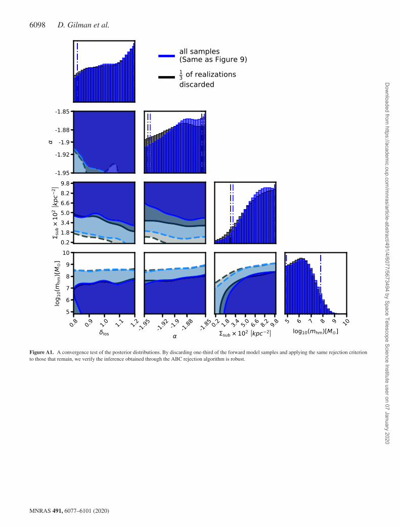
6098 D. Gilman et al.
Figure A1. A convergence test of the posterior distributions. By discarding one-third of the forward model samples and applying the same rejection criterionto those that remain, we verify the inference obtained through the ABC rejection algorithm is robust.
MNRAS 491, 6077–6101 (2020)
Dow
nloaded from https://academ
ic.oup.com/m
nras/article-abstract/491/4/6077/5673494 by Space Telescope Science Institute user on 07 January 2020

Strong lensing constraints on dark matter 6099
Figure A2. A convergence test of the posterior distributions assuming CDM. Like Fig. A1, one-third of the samples are discarded and the same number ofrealizations are accepted into the posterior.
APPENDIX B: O BTAINING DEFLECTO RREDSHIFTS
The quads PS J1606 and WGD J0405 do not have measuredspectroscopic redshifts, so we use photometry from Shajib et al.(2019) to obtain photometric redshift estimates. The photometryfrom Shajib et al. (2019) comes in three bands: F160W, F814W,and F475X with magnitude uncertainties of 0.1–0.3 dex. We usethe software package EAZY (Brammer et al. 2008), and restrict thetemplates to only consider the SEDs for early-type galaxies, whichare 90 per cent of galaxies acting as strong lenses. We verify thisprocedure is accurate by applying it to other deflectors in sampleanalysed by Shajib et al. (2019) that have measured spectroscopicredshifts, and then proceed to derive PDFs for deflector redshifts inthe systems PS J1606 and WGD J0405.
The results are shown in Fig. B1. The top row shows four quadsfrom the sample analysed in Shajib et al. (2019) with measuredspectroscopic redshifts, and the bottom row shows the PDF’s outputby EAZY for the systems PS J1606 and WGD J0405.
The system WFI 2026 does not have a photometric redshift, andthe photometry available in the literature comes in only one or twobands with larger uncertainties. For this system, we use the equationfor isothermal mass profiles relating the Einstein radius REin, sourceredshift zs, lens redshift zd, velocity dispersion σ , and speed oflight c
REin = 4π(σ
c
)2 Dds(zd, zs)
Ds(zs), (B1)
where Dds and Ds are angular diameter distances between the lensand the source, and the observer and the source, respectively.
MNRAS 491, 6077–6101 (2020)
Dow
nloaded from https://academ
ic.oup.com/m
nras/article-abstract/491/4/6077/5673494 by Space Telescope Science Institute user on 07 January 2020

6100 D. Gilman et al.
Figure B1. PDFs for main deflector redshifts computed with the softwareEAZY and photometry from Shajib et al. (2019), restricting the photometrytemplates to those of early-type galaxies. The top rows show four applica-tions of this procedure to quads with measured spectroscopic redshifts (reddotted lines). The bottom row shows the results of this procedure, using thesame photometry and template assumptions, applied to the quads PS J1606and WGD J0405, which do not have spectroscopic redshift measurements.
Figure B2. The PDF for the deflector redshift of WFI 2026 obtained byassuming a velocity dispersion of 240 ± 30 km s−1 and a roughly isothermalmass profile.
We sample a Gaussian distribution of velocity dispersions typicalof early-type galaxies 240 ± 30kms−1, evaluate the right-hand sideof equation (B1), and numerically solve for the lens redshift thatyields the resulting angular diameter distance. The resulting PDFshown in the bottom right panel of Fig. B2 peaks around zd =1, for the measured values REin = 0.67 arcsec, zs = 2.2. We haveexperimented with placing WFI 2026 at various specific redshifts,but find the posteriors for �sub, δlos, α, and mhm are unchangedwithin the uncertainties.
APPENDI X C : DATA
We summarize the data used in this analysis, and the referencesfor the astrometry, fluxes or flux ratios, and the correspondinguncertainties, and satellite galaxies or nearby nearby deflectors inTable C1.
MNRAS 491, 6077–6101 (2020)
Dow
nloaded from https://academ
ic.oup.com/m
nras/article-abstract/491/4/6077/5673494 by Space Telescope Science Institute user on 07 January 2020

Strong lensing constraints on dark matter 6101
Table C1. The data used in this analysis. Letters A–D correspond to the lensed images, while G is thegalaxy light centroid. The priors sampled for the satellite galaxies or nearby deflectors are quoted inTable 2. Discovery papers are marked with a †.
Lens Image dRA dDec. NL flux
WGD J0405–3308 A 1.066 ± 0.003 0.323 ± 0.003 1.00 ± 0.04Nierenberg et al. (2019) B 0 ± 0.003 0 ± 0.003 0.65 ± 0.04†Anguita et al. (2018) C 0.721 ± 0.003 1.159 ± 0.003 1.25 ± 0.03
D − 0.157 ± 0.003 1.021 ± 0.003 1.17 ± 0.04G 0.358 ± 0.05 0.567 ± 0.05 –
HE0435–1223 A 2.424 ± 0.008 0.792 ± 0.008 0.97 ± 0.05Nierenberg et al. (2017) B 1.458 ± 0.008 − 0.456 ± 0.008 0.98 ± 0.049Wong et al. (2017) C 0 ± 0.008 0 ± 0.008 1 ± 0.048†Wisotzki et al. (2002) D 0.768 ± 0.008 1.662 ± 0.008 0.54 ± 0.056
G 1.152 ± 0.05 0.636 ± 0.05 –
RX J0911+0551 A 0 ± 0.003 0 ± 0.003 0.56 ± 0.04Nierenberg et al. (2019) B 0.258 ± 0.003 0.405 ± 0.003 1.00 ± 0.05†Bade et al. (1997) C − 0.016 ± 0.003 0.959 ± 0.003 0.53 ± 0.04Blackburne et al. (2011) D − 2.971 ± 0.003 0.791 ± 0.003 0.24 ± 0.04
G − 0.688 ± 0.05 0.517 ± 0.05 –
B1422+231 A 0.387 ± 0.005 0.315 ± 0.005 0.88 ± 0.01Nierenberg et al. (2014) B 0 ± 0.005 0 ± 0.005 1.00 ± 0.01†Patnaik et al. (1992) C − 0.362 ± 0.005 − 0.728 ± 0.005 0.474 ± 0.006
D 0.941 ± 0.01 − 0.797 ± 0.01 –G 0.734 ± 0.01 − 0.649 ± 0.01 –
PS J1606–2333 A 1.622 ± 0.003 0.589 ± 0.003 1.00 ± 0.03Nierenberg et al. (2019) B 0 ± 0.003 0 ± 0.003 1.00 ± 0.03Shajib et al. (2019) C 0.832 ± 0.003 − 0.316 ± 0.003 0.59 ± 0.02†Lemon et al. (2018) D 0.495 ± 0.003 0.739 ± 0.003 0.79 ± 0.02
G 0.784 ± 0.05 0.211 ± 0.05 –
WFI 2026–4536 A 0.164 ± 0.003 − 1.428 ± 0.003 1.00 ± 0.02Nierenberg et al. (2019) B 0.417 ± 0.003 − 1.213 ± 0.003 0.75 ± 0.02†Morgan et al. (2004) C 0 ± 0.003 0 ± 0.003 0.31 ± 0.02
D − 0.571 ± 0.003 − 1.044 ± 0.003 0.28 ± 0.01G − 0.023 ± 0.05 − 0.865 ± 0.05 –
WFI 2033–4723 A − 2.196 ± 0.003 1.260 ± 0.003 1.00 ± 0.03Nierenberg et al. (2019) B − 1.484 ± 0.003 1.375 ± 0.003 0.65 ± 0.03Vuissoz et al. (2008) C 0 ± 0.003 0 ± 0.003 0.50 ± 0.02†Morgan et al. (2004) D − 2.113 ± 0.003 − 0.278 ± 0.003 0.53 ± 0.02
G − 1.445 ± 0.05 2.344 ± 0.05 –
WGD 2038–4008 A − 2.306 ± 0.003 1.708 ± 0.003 1.00 ± 0.01Nierenberg et al. (2019) B 0 ± 0.003 0 ± 0.003 1.16 ± 0.02†Agnello et al. (2018) C − 1.518 ± 0.003 0.029 ± 0.003 0.92 ± 0.02
D − 0.126 ± 0.003 2.089 ± 0.003 0.46 ± 0.01G − 0.832 ± 0.05 1.220 ± 0.05 –
This paper has been typeset from a TEX/LATEX file prepared by the author.
MNRAS 491, 6077–6101 (2020)
Dow
nloaded from https://academ
ic.oup.com/m
nras/article-abstract/491/4/6077/5673494 by Space Telescope Science Institute user on 07 January 2020