1500 K Street NW, Suite 850 Washington, DC 20005

Daniel SchneiderKristen Harknett

http://equitablegrowth.org/working-papers/schedule-instability-and-unpredictability/

Washington Center forEquitable Growth

Working paper series

September 2016

© 2016 by Daniel Schneider and Kristen Harknett. All rights reserved. Short sections of text, not to exceed two paragraphs, may be quoted without explicit permission provided that full credit, including © notice, is given to the source.

Schedule instability and unpredictability and worker and family health and wellbeing

Schedule Instability and Unpredictability and Worker and Family Health and Wellbeing  

Daniel Schneider and Kristen Harknett  

September 2016 

 

 

Abstract The American labor market is increasingly unequal, characterized by extraordinary returns to work at the 

top of the market but rising precarity and instability at the bottom of the market. In addition to low wages, 

short tenure, few benefits, and non­standard hours, many jobs in the retail and food service industries are 

characterized by a great deal of instability and unpredictability in work schedules. Such workplace 

practices may have detrimental effects on workers. However, the lack of existing suitable data has 

precluded empirical investigation of how such scheduling practices affect the health and wellbeing of 

workers and their families. We describe an innovative approach to survey data collection from targeted 

samples of service­ sector workers that allows us to collect previously unavailable data on scheduling 

practices and on health and wellbeing. We then use these data to show that exposure to unstable and 

unpredictable schedules is negatively associated with household financial security, worker health, and 

parenting practices.  

 

 

Daniel Schneider  Kristen Harknett  

University of California, Berkeley University of Pennsylvania 

Department of Sociology Department of Sociology 

djschneider@berkeley.edu harknett@sas.upenn.edu 

 

 

We gratefully acknowledge grant support from the Washington Center for Equitable Growth, the Institute 

for Research on Labor and Employment, the UC Berkeley School of Public Health, and the Hellman 

Fellows Fund. We are grateful to Liz Ben­Ishai, Annette Bernhardt, Michael Corey, Sarah Crow, Rachel 

Deutsch, Dennis Feehan, Carrie Gleason, Heather Hill, David Harding, Julie Henly, Ken Jacobs, Susan 

Lambert, Sophie Moulllin, Jesse Rothstein, Matt Salganik, Stewart Tansley, Joan Williams, and 

participants in the Aspen Institute’s EPIC convening for very useful feedback and discussion. We 

received excellent research assistance from Carmen Brick, Alison Gemmill, Sigrid Luhr, and Robert 

Pickett. A previous version of this work was presented at UC Berkeley’s Institute for Research on Labor 

and Employment.  

 

 

 

 

 

Introduction

The American labor market is increasingly unequal, characterized by extraordinary returns to work

at the top of the market but rising precarity and instability at the bottom of the market. This

precarity is multi-dimensional, characterized by low-wages, few benefits, short tenure, contingent

employment, and non-standard schedules. While the consequencs of these dimensions of precarity

have been studied, scholars, policy makers, workers, and advocates have recently documented a new

set of precarious employment practices related to work scheduling that may have serious negative

e↵ects on workers and their families. However, very little research has traced how these scheduling

practices a↵ect health and wellbeing.

Many service-sector employers now use a combination of human resource management strate-

gies to closely align sta�ng with demand. Under this system, workers receive their weekly work

schedules as little as a few days in advance, their scheduled work hours and work days may change

substantially week-to-week, and workers may have their shifts changed, cancelled, or added at the

last minute (Golden, 2001; Appelbaum et al., 2003; Clawson and Gerstel, 2015). Recent estimates

suggest that nearly 90% of hourly retail workers experience such instability (Lambert et al., 2014).

These scheduling practices have gained attention in the media with many journalistic accounts

of the hardships imposed by unstable and unpredictable schedules (Singal, 2015; White, 2015;

Kantor, 2014; Strauss, 2015). These accounts suggest, and related research supports the idea, that

schedule instability may increase the volatility of household economic resources, increase stress

and uncertainty, destabilize people’s daily lives, interfere with combining work with schooling or

secondary jobs, and prevent the establishment of regular schedules of personal and dependent care.

Schedule and hours instability may then negatively a↵ect workers’ health behaviors and mental and

physical health. These work scheduling practices may also transmit disadvantage across generations.

Children whose parents work unstable and unpredictable schedules may be subject to inconsistent

care arrangements and frequent disruptions to their routines and time with parents.

However, while there is evidence that other dimensions of precarious work – such as stable, but

non-standard hours – negatively a↵ect health and wellbeing, the evidence base on the e↵ects of un-

stable and unpredictable scheduling practices is more limited. Data sources containing information

on both work scheduling and health outcomes are rare and workers in low-wage unstable jobs are

di�cult to sample.

1

Nevertheless, policy makers have been actively pursuing changes to local labor regulations and,

beginning in the Fall of 2016, four large cities are expected to pass local labor laws regulating

unstable and unpredictable schedules (Ben-Ishai, 2015a). Large retailers, including Walmart, are

independently making or contemplating changes to company policies.

We use an innovative survey method to collect data from 6,476 hourly non-managerial retail

workers in the United States. Our study, the Retail Work and Family Life Study (RWAFLS), is

unique in collecting detailed measures on schedule instability and unpredictability as well as mea-

sures of worker and family health, social wellbeing, and household financial security for a national

sample of retail workers. This paper describes our unique data collection method and our meth-

ods for assessing and mitigating sample selectivity, then reports on the associations between work

scheduling practices and worker health and wellbeing. We find that unstable and unpredictable

work schedules are negatively associated with a number of dimensions of worker and family well-

being including household economic insecurity, psychological distress, and reductions in parental

time with children. These relationships have long been suspected but have not been systematically

documented in large-scale empirical research.

The set of scheduling practices we examine – varying number of hours, variable schedules, and

limited advance notice of work schedules – would likely be changed by proposed local legislation

and proposed shifts in company practices. We conclude our paper by considering our findings in

the context of proposed scheduling legislation and changes to company practice.

Background

Employment Precarity

One important dimension of socio-economic status is the nature of one’s paid work, and influential

sociological research has shown increasing employment precarity since the 1970s, which has been

defined as an increase in work that is “uncertain, unpredictable, and risky from the point of view

of the worker” (Kalleberg, 2009, p. 2). While this increase in precarity has been widespread, those

at the bottom of the income and occupational distribution have fared the worst. Fligstein and Shin

(2004) report on a bifurcation of the labor market between the 1970s and 1990s in which workers

with lower levels of educational attainment experienced declines in wages, declines in benefits such

2

as health insurance and pensions, and declines in job security and job satisfaction. Fligstein and

Shin refer to this set of changes as the “insecuritization of work for those at the bottom” (p. 402).

These declines in job quality since the 1970s have been accompanied by a rise in non-standard

work hours that encompass evenings, nights, and weekends - hours that are di�cult to reconcile

with parenting responsibilities. Presser (1999) documented the prevalence of these non-standard

shifts two decades ago and was prescient in predicting that these non-standard shifts would continue

to increase in their prevalence (McMenamin 2007).

Unstable and Unpredictable Work Schedules

Scholars and policy makers have more recently identified a new form of employment precarity in the

low-wage service sector rooted in a set of unstable and unpredictable scheduling practices. Under

this system, workers receive their weekly work schedules as little as a few days in advance, their

scheduled work hours and work days may change substantially week-to-week, and workers may

then have their shifts changed, cancelled, or added at the last minute (Golden, 2001; Appelbaum

et al., 2003; Clawson and Gerstel, 2015).

This set of practices allows employers to e↵ectively transfer financial risk to their employees.

Rather than commit to a set of stable employee schedules, employers now seek to maintain as lean

sta�ng as possible and do so by scheduling workers for minimal regular hours, adding shifts at the

last minute, asking workers to leave shifts early, and requiring “on call” shifts (Houseman 2001).

Employers are thus able to avoid paying for idle sta↵ time. In turn, employees encounter substantial

uncertainty about when and how much they will work. In this way, unpredictable and unstable

scheduling practices are yet another domain in which risk is transferred from large institutional

actors to households (Hacker, 2006).

Unstable and unpredictable work schedules are now common in the service sector (Golden, 2001;

Appelbaum et al., 2003; Enchautegui et al., 2015) and can be found among low-wage workers in

other industries as well, such as health care (Clawson and Gerstel, 2015). Recent estimates show

that 87% of early-career retail workers reported instability in their work hours from week to week

over the past month. Of those retail workers who reported unstable work hours, the fluctuations

were substantial, averaging almost 50% of their usual weekly hours (Lambert et al., 2014).

These arrangements are widespread and qualitatively distinct from low-wage stable non-standard

3

work. Early research has shown that this instability is highly salient for workers (i.e. Luce et al.,

2014) and may even be a more important predictor of wellbeing than working non-standard hours

(Henly and Lambert, 2014a). However, there is very little research that directly examines the social

consequences of unstable and unpredictable work.

Expected E↵ects of Unstable Schedules on Wellbeing

Although there is little prior research that directly examines the relationship between schedule

unpredictability and instability and health and wellbeing for service-sector workers, theory and

prior research provide several reasons to expect that unpredictable and on-call scheduling for hourly

employees will have a range of negative e↵ects.

Most broadly, the positive relationship between socioeconomic status and health is robust and

well established. Those with lower incomes and less education have shorter life expectancy, higher

rates of morbidity, depression, and health risk behaviors, and socioeconomic status has been the-

orized to be a “fundamental cause” of health outcomes (Link and Phelan, 1995). To the extent

that exposure to unstable and unpredictable work schedules is another dimension of socio-economic

status, we might expect similar ill e↵ects.

Scholars have also long been concerned with the e↵ects of precarious work specifically on health

and wellbeing. Prior research has carefully documented the e↵ects of non-standard work schedules

on adult wellbeing (i.e. Presser, 2003; Presser, 1999; Wight, Raley, and Bianchi, 2008) and on child

outcomes and parenting (i.e. Joshi and Bogen, 2007; Han, 2005; Miller and Han, 2008; Morsy and

Rothstein, 2015; Scott et al., 2004). Separate research in sociology and epidemiology has shown

how limited flexibility in the workplace negatively a↵ects the health and wellbeing of white collar

workers (Marmot et al., 1997; Ala-Mursula et al., 2002; Hurtado et al,, 2016; Olson et al., 2015;

Davis et al., 2015; Moen et al., 2016).

But, the evidence base on the e↵ects of unstable and unpredictable schedules on the wellbe-

ing of hourly workers and their families is much thinner. A first order question relates to how

workers perceive their schedules. While limited advanced notice and variable shift timing might,

a priori, appear undesirable, some suggest that rather than embodying harmful instability, these

scheduling practices are a reflection of employee desire for flexibility (Hatamiya, 2015). Qualitative

research on workers with unstable and unpredictable schedules suggests that these practices are

4

perceived negatively (Henly, Shaefer, and Waxman, 2006). But, there is little large scale survey

data demonstrating whether workers would prefer more stable schedules.

Second, unpredictable and unstable work schedules may have negative consequences for house-

hold economic security. Variable hours may, mechanically, lead to income volatility, especially if

that variability makes it di�cult for workers to hold secondary jobs that might otherwise be used

to smooth earnings. Prior research has shown that schedule instability leads to economic insecurity

(Ben-Ishai, 2015b; Golden, 2015, Haley-Lock, 2011; Luce et al., 2014; Zeytinoglu et al., 2004). In

a 2013 survey of workers with low to moderate income, among those who reported income volatil-

ity, having an irregular work schedule was the most common reason given (Federal Reserve Board

2014). Similarly, in a financial diary study of 235 households, negative income shocks were common

and a drop in work hours was one of the main culprits (Murdoch and Schneider 2014).

Unpredictable and unstable schedules may also have negative e↵ects on worker and family health

and wellbeing. These e↵ects could be caused by economic instability. Additionally, such scheduling

practices also appear to interfere with daily routines and causes chronic stress and uncertainty

(Ben-Ishai, 2015b; Golden, 2015, Haley-Lock, 2011; Luce et al., 2014; Morsy and Rothstein, 2015;

Zeytinoglu et al., 2004). These factors, in turn, have been shown to be negatively related to

health and wellbeing. In terms of worker wellbeing, prior research indicates that income volatility

negatively a↵ects sleep and food su�ciency (Wight, Raley, and Bianchi, 2008; Leete and Bania,

2010). Elevated levels of work stress are also related to unhealthy behaviors such as smoking

(Kouvonen et al., 2005) and alcohol consumption (Harris and Fennell, 1998). Research has found

that income volatility and job insecurity are both associated with worse self-rated health (Halliday,

2007; Goh, Pfe↵er, and Zenios, 2015).

In terms of child wellbeing and parenting, prior research has also found income volatility and

economic uncertainty are associated with parenting stress (Wolf et al., 2014), harsh parenting

(Gassman-Pines, 2013; Schneider et al., 2013), less parenting time (Wight et al., 2008), and poor

child outcomes (Gennetian et al., 2015; Schneider et al., 2013; Miller and Han, 2008). In addition,

several studies have documented a direct relationship between unstable work schedules and incon-

sistent and low quality child care arrangements (Ben-Ishai et al., 2014; Enchautegui, et al., 2015;

Henly and Lambert, 2005; Luce et al., 2014; Morsy and Rothstein, 2015; Williams and Boushey,

2010) and between disrupted schedules at home for children and lower quality parental interactions

5

(Henley, Shaefer, and Waxman, 2006).

Although data on scheduling practices and health and wellbeing outcomes are limited, prior

research provides indirect evidence to suggest that these scheduling practices are linked with a

range of financial, health, and wellbeing outcomes. The prior research evidence leads us to the

following set of hypotheses:

1. We hypothesize that workers exposed to unstable scheduling practices will be more likely toexpress a desire for stable work hours.

2. We expect that unstable and unpredictable schedules will be negatively related to householdeconomic security as seen in income volatility and measures of financial strain.

3. We predict that exposure to these scheduling practices may interfere with sleep and depressself-rated health and emotional wellbeing.

4. For working parents, we hypothesize that unstable work schedules will reduce developmentaltime with children and increase parenting stress.

We propose an innovative approach to data collection and estimation that will allow us to directly

examine the relationship between unstable and unpredictable schedules and worker attitudes, house-

hold financial security, health and wellbeing, and parenting.

Data and Methods

The lack of existing research on how unpredictable schedules a↵ect worker and family wellbeing

stems from a lack of available data. There are three interrelated limitations of existing data: (1) few

data sets include measures of scheduling practices, (2) data sets that include measures of scheduling

practices rarely include measures of wellbeing, and (3) existing data cannot be used to describe the

scheduling practices at the large retail firms that are at the center of policy debate and organizing

activity.

First, few data sets actually measure scheduling practices. While scholars have developed an

accepted set of survey items to measure unpredictable and unstable work schedules (Lambert and

Henly, 2014b), these items are new and have not yet been included on the large scale governmental

surveys that are the mainstay of social science research. For instance, the American Community

Survey and the Decennial Census both contain large numbers of retail workers, but do not measure

advance notice of schedules or variation in weekly hours. Other smaller-scale data sets such as the

Panel Study of Income Dynamics, the National Health Interview Survey, the National Longitudinal

6

Study of Youth-79, and the National Longitudinal Study of Adolescent to Adult Health also contain

little information on scheduling practices.

Second, those surveys that contain information on scheduling practices generally lack informa-

tion on health and wellbeing - key outcomes of interest. For instance, the Current Population

Survey included a set of scheduling measures in a special module in 2004 (and includes a recurrent

question on hours worked that contains an option to report that hours vary), but does not include

measures of worker or family health or wellbeing. A series of state and national surveys conducted

by the Employment Instability Network contain detailed measures of scheduling instability and

unpredictability, but no measures of health and wellbeing. Those surveys that do contain detailed

outcome data – such as NHIS, Fragile Families, Add Health, and others – lack good measures of

scheduling practices.

One important exception is the 2011 and 2013 waves of the National Longitudinal Survey of

Youth - 1997 (NLSY-97). In those two waves, the NLSY-97 contained items that gauged amount

of advance notice of schedules that the respondent received at work, the degree of control the

respondent had over her schedule, and the week-to-week variability in the respondent’s work hours.

The NLSY-97 also contains useful measures of adult health and wellbeing. However, the NLSY-97

is limited to a specific cohort of workers - all of whom were born between 1975 and 1982 and were

aged 29 to 36 in 2011. Because the NLSY-97 is designed to be nationally representative of that age

cohort, the sample size of workers in the retail industry is limited, with 763 respondents working in

retail in 2011.1 Further, some portion of these retail industry workers are in managerial positions,

and the employer name is not available in the data.

Finally, though policy attention and organizing is focused on regulating large chain retailers,

there is no data that can be used to actually describe scheduling practices at these companies.

Administrative data, which is at su�cient scale to describe practices at individual employers,

does not contain measures of schedules or of worker health and wellbeing. Surveys that measure

scheduling practices either do not collect information on the names of individual employers or lack

any substantial number of cases within particular employers. In sum, there is an acute lack of data

that contains measures of scheduling and outcomes of interest for su�ciently large samples of retail

1From the NLSY-97 documentation of the industry codes for respondents’ current or most recent job in Round 14.https://www.nlsinfo.org/content/cohorts/nlsy97/topical-guide/employment/industry-occupation-tables

7

workers. A significant challenge in collecting this data is the e↵ective recruitment of large samples

of retail workers at reasonable cost.

Survey Methodology

We use an innovative method of collecting web-based surveys from a population of low-wage service-

sector workers. We use audience-targeted advertisements on Facebook to recruit respondents to a

survey. Facebook collects extensive data on its users by harvesting user-reported information and

inferring user characteristics from activity. Facebook then allows advertisers to use this data at the

group level to target advertisements to desired audiences. We take advantage of this infrastructure

to target survey recruitment messages to active users on Facebook who (1) reside in the United

States, (2) are between the ages of 18 and 50, and (3) list one of several large retail companies as

their employer.

This approach to survey data collection departs from traditional probability sampling methods

and some have raised reasonable questions about such approaches (Groves, 2011; Smith, 2013). One

possible source of bias arises from our sampling frame – Facebook users. While earlier research

noted selection into Facebook activity (Couper, 2011), recent estimates show that approximately

80% of Americans age 18-50 are active on Facebook (Perrin, 2015). Thus, the sampling frame is

now on par with coverage of telephone-based methods (Christian et al., 2010).

Our approach is innovative, but not without precedent. Faced with declining response rates

to traditional probability sample surveys, an emerging body of work has demonstrated that non-

probability samples drawn from non-traditional platforms, in combination with statistical adjust-

ment, yield similar distributions of outcomes and estimates of relationships as probability-based

samples. This work has drawn data from Xbox users (Wang et al., 2015), Mechanical Turk (Goel,

Raod, and Sro↵, 2015; Mullinix et al., 2016), and Pollfish (Goel et al., 2015). Yet, of all of these

platforms, Facebook is the most commonly and widely used by the public (Perrin, 2015). In recent

prior work, Bhutta (2012) reports on using Facebook to recruit Catholic respondents to a survey.

However, her approach di↵ers starkly from ours. Rather than using targeted advertising, as we

do, Bhutta (2012) issued survey invitations to members of Catholic a�nity groups on Facebook

and then relied on chain referrals to recruit additional respondents. This approach initially selects

on the intensity of Catholic identity to recruit and then introduces problems of correlated errors

8

through the chained referrals.

Below, we discuss the logistics of our alternative approach using targeted advertising in greater

detail, and then describe several steps that we take to guard against sample selection bias.

Detailed Survey Methodology

We purchase advertisements on the Facebook platform, paying on a cost-per-click basis (mean-

ing that we incur expenses against our daily advertising budget every time a user clicks on our

advertisement, but not every time a user sees our advertisement).

We define our target audience by age (18-50) and employer and systematically vary the ad-

vertising message. Varying the messages accomplishes two important goals. First, by varying the

messages, we increase our click-through-rate (CTR). Second, as described in detail below, we use

pairs of distinct and opposing messages that are designed to appeal to respondents who di↵er on

some unobserved characteristic that could influence our results.

Respondents who click on the link in our advertisement are redirected to an online survey hosted

through the Qualtrics platform. The front page of the survey contains introductory information

and a consent form. Respondents provide consent by clicking to continue to the survey instrument.

The specific survey items are detailed below.

Each advertisement is targeted to the employees of a particular large retail company. We selected

these companies from the top 15 largest retailers by sales in the United States (National Retail

Federation, 2015). We first exclude Amazon.com (#8) and Apple Stores/iTunes (#13) from this

list because their rank is the product exclusively or partially of internet sales rather than traditional

brick-and-mortar retail operations. We then selected eight companies from the remaining 13.

We placed these survey recruitment advertisements on Facebook between January and June

of 2016. We purchased advertisements on a cost-per-click basis. Our advertisements generated

1,284,428 views and 28,410 clicks through to our survey. We calculate our overall click-through-

rate as 2.21%. Of those continuing through to our survey, 11,932 consented to begin the survey.

Our most liberal response rate then is that 42% of those who clicked began the survey and that 0.9%

of users who saw one of our advertisements began a survey. There was, however, some attrition

over the course of the survey. Our adjusted response rate, taking only fully completed surveys

(surveys where respondents advanced through to the end of the survey and provided their email

9

address for follow-up) as the numerator, is that 18% of users who clicked completed the survey and

0.4% of users who saw one of our advertisements completed a survey. These response rates are far

lower than in traditional survey methods. However, a sample such as ours would be di�cult if not

impossible to reach through traditional methods. Nevertheless, we are attentive to issues of sample

selectivity and address potential bias by weighting and testing for selection on unobservables.

Methods of Mitigating Bias

As noted above, Facebook use is so widespread as to diminish concerns about its use as a sampling

frame. However, a second source of bias arises from non-random non-response to the recruitment

advertisement. We investigate and ameliorate such potential response biases using both accepted

and more novel methods.

First, statisticians have developed a set of post-stratification and weighting methods that can

be used to generate accurate estimates from this type of data (Wang et al., 2015; Goel et al.,

2016). This approach allows us to adjust our data to account for discrepancies in the demographic

characteristics of our sample compared with the characteristics of a similar target population of

workers captured in the high-quality probability sample survey data collected by the American

Community Survey (ACS) and the Current Population Survey (CPS). In particular, compared to a

similar sample of workers in the ACS or CPS, our sample over-represents women and non-Hispanic

whites. We construct weights that when applied allow our sample to more closely mirror the

population of retail workers we are aiming to represent.

We post-stratify our data into a set of 40 cells defined by the characteristics of age, gender, and

race/ethnicity. We construct weights by comparing distributions across these 40 cells in our data

to distributions in the ACS and CPS data. We then construct weights such that within a group the

sum of weights within the Facebook survey equals the total number of observations in that group in

the ACS or CPS. We then adjust weights so that they sum to the original sample size in our survey

sample so as not to a↵ect standard errors. After applying the weights, the demographic composition

of our sample on these three characteristics matches the composition of the corresponding samples

in the ACS and CPS. Further details on our weighting approach are provided in the Appendix.

Table 1 compares a set of descriptive statistics for the unweighted analysis sample (column 1),

the analysis sample weighted based on the ACS (column 2), the analysis sample weighted based

10

on the CPS (column 3), and tabulations of the same characteristics for the target population from

the ACS (column 4) and CPS (column 5). Before weighting, our sample is disproportionately

female and White, non-Hispanic as compared to the ACS (column 4) and CPS (column 5) samples.

However, the age distribution of our unweighted data is not notably di↵erent from that of the

ACS or CPS samples. Our weighted sample (columns 2 and 3) is, by construction, identical to

the samples from the ACS and CPS on gender, age, and race/ethnicity. We do not weight on

education and we see that while the share of respondents with a BA or more matches that of the

ACS and CPS, the share with some college is somewhat higher than in those data. However, the

share enrolled in school is consistently about 25%.

This approach can e↵ectively adjust for bias in observed characteristics, including for data

with much more extreme demographic bias than we observe in our data (i.e. Wang et al., 2015).

However, this approach assumes that within narrowly defined cells, the sample is drawn randomly.

It is possible, however, that other unobserved biases exist in sample selection.

Second, rather than speculate about such forms of non-specific bias, we generate hypotheses

about potential, specific unobserved characteristics that might both alter survey response and bias

the relationship between schedule instability and health and wellbeing outcomes. We then run

advertisements that elicit these “unobservable” characteristics in their messaging (for instance,

contrasting an advertising message referencing insu�cient work hours with one referencing over-

work) and examine if the relationship between schedule instability and health and wellbeing varies

for respondents recruited through these opposing channels.

Key Measures

We fielded an online survey containing approximately 70 questions for workers without children,

and 90 questions for working parents. The survey was divided into five modules. The first module

contained information on job characteristics, the second on household finances, the third on worker

health and wellbeing, the fourth on parenting and child wellbeing (asked only of parents with

children in the home), and the fifth on demographics.

11

Independent Variables: Schedule Instability and Unpredictability

We measure the instability of respondents’ schedules with 3 key items. First, we ask respondents

to classify their usual schedule as a regular day shift, a regular evening shift, a regular night shift, a

variable schedule, a rotating shift, or some other arrangement. Second, we ask respondents for the

amount of advance notice they are given of their schedule, di↵erentiating one week of notice or less,

1-2 weeks, 2-3 weeks, 3-4 weeks, or 4 weeks or more (we collapse these last two categories into one

since few respondents reported 4 weeks or more of notice). Third, we calculate a measure of hour

volatility by asking respondents to report the most and the fewest weekly hours they worked over

the past 4 weeks and taking the di↵erence in hours divided by the maximum weekly hours. These

items have been carefully developed and tested by the Employment Instability Network (Henly and

Lambert, 2014b).

Dependent Variables

We examine four groups of outcome variables: (1) work-related attitudes, (2) household financial

security, (3) adult health and wellbeing, and (4) parenting. The questions used to measure outcomes

in each of these domains are generally drawn from existing surveys, including the Behavioral Risk

Factor Surveillance System and the Fragile Families and Child Wellbeing survey.

Work-Related Attitudes. We assess the relationship between our measures of schedule unpre-

dictability and instability and three measures of attitudes. First, respondents are asked to indicate

their agreement with the statement “I would like to work more hours,” (Strongly Agree (SA), Agree,

Disagree, or Strongly Disagree (SD)). Second, respondents are asked to indicate their agreement

with the statement, “I would like to work more regular hours” (SA to SD). The first is designed

to gauge satisfaction with the number of hours and the second with the regularity of those hours.

For each of these measures, we create a dichotomous variable separating those who strongly agree

or agree from those who disagree or strongly disagree.

Household Financial Security. We measure three dimensions of household financial security.

First, we gauge household income volatility by directly asking respondents, “would you say that

week to week your household income is basically the same or goes up and down.” We treat this

as a dichotomous variable. Second, we ask respondents, “in a typical month, how di�cult is

it for you to cover your expenses and pay all your bills” and ask respondents to rate it as very

12

di�cult, somewhat di�cult, or not at all di�cult. We recode responses into a dichotomous variable

contrasting “very di�cult” with “somewhat” or “not at all di�cult.” Third, we create an additive

index of household economic hardships experienced in the 12 months prior to survey composed of

the following indicators: using a food pantry, going hungry, not paying utilities, taking an informal

loan, moving in with family or friends, staying in a shelter, or deferring needed medical care.

Worker Health and Wellbeing. We measure workers’ self-rated health using a five-category

response scale (excellent, very good, good, fair, or poor) recoded to a dichotomous variable con-

trasting excellent or very good health with good, fair, or poor self-rated health. We gauge general

emotional wellbeing by asking respondents, “taken all together, how would you say things are these

days? Would you say you are, (1) very happy, (2) pretty happy, or (3) not too happy.” We recode

responses into a dichotomous variable contrasting very or pretty happy with not too happy. We

also measure self-rated sleep quality as very good, good, fair or poor and create a dichotomous

variable contrasting very good or good sleep with fair or poor sleep. Finally, we use the Kessler-6

index of non-specific psychological distress, assessing both the total score as a continuous variable

(ranging from 0 to 24) and creating a dichotomous measure of serious psychological distress that

separates scores below 13 from those between 13 and 24 (Kessler et al., 2003).

Parenting. For working parents who live with children under the age of 15, we ask about time

spent with children engaging in the following 6 activities: eating meals together, watching television

together, playing video games with children, homework help or reading, active play indoors, and

active play outdoors. Respondents rated each activity as occurring never (4), 1-2 times per month

(3), once a week (2), several times a week (1), or everyday (0) and we created a summative index

ranging from 0 to 24 to capture the intensity of parental time with children. Note that higher

values on this index signal less time spent with children.

We also measure parenting stress. Respondents are asked their level of agreement, either

strongly agree, agree, disagree, or strongly disagree, with four statements: (1) being a parent

is harder than I thought it would be, (2) I feel trapped by my responsibilities as a parent, (3) I

find that taking care of my children is much more work than pleasure, and (4) I often feel tired,

worn out, or exhausted from raising a family. We then create a summative index of the responses

that ranges from 0 (strongly disagree with all four statements) to 12 (strongly agree with all four

statements), such that higher values indicate greater parenting stress.

13

Controls

The rise in precarious employment involved declines in wages and worsening of employment con-

ditions more generally, in addition to the changes in scheduling practices. Therefore, to isolate

the e↵ects of scheduling practices from other features of precarious employment, all of our models

control for hourly wage, average work hours in the last month, household income, and job tenure.

We also control for a set of demographic characteristics composed of age, race/ethnicity, gender, ed-

ucational attainment, school enrollment, marital status, and presence of children in the household.

These individual characteristics help to control for selection into jobs with particular attributes.

Last, we include employer and state fixed e↵ects in our models, which control for any time-invariant

characteristics of employers and states.

Analytic Models

We estimate associations between our three key measures of schedule instability (variation in weekly

hours, schedule type, and advanced notice) and four domains of outcomes: work-related attitudes,

household financial security, adult health and wellbeing, and parenting. While these estimates

are not causal, we note that by design our sample has limited heterogeneity: everyone is a non-

managerial hourly retail worker and we control for economic and demographic characteristics as

well as for state and employer fixed-e↵ects. We estimate the following model:

Yi = ↵+ �Xi + �Ji + µ+ ! + ✏i (1)

where, our outcome of interest, Y for individual i, is regressed on a set of control variables, X,

and a set of job scheduling characteristics, J described above. The coe�cients of interest are rep-

resented by � and summarize the relationship between work schedules and the wellbeing of workers

and their families in terms of the dependent variables described above. The set of individual-level

controls, Xi, will include respondent-level measures of race/ethnicity, age, education, nativity, mar-

ital status, hourly wage, average work hours in the past month, household income, job tenure, and

household composition. The terms µ and ! represent employer and state fixed e↵ects, which con-

trol for unobserved time-invariant characteristics of employers or states. Equation (1) shows the

OLS model that we use for continuous outcomes. For dichotomous outcomes, we estimate logistic

14

regression models where the log odds of the dependent variable is regressed on the set of predictors

shown in equation (1) and the error term drops out.

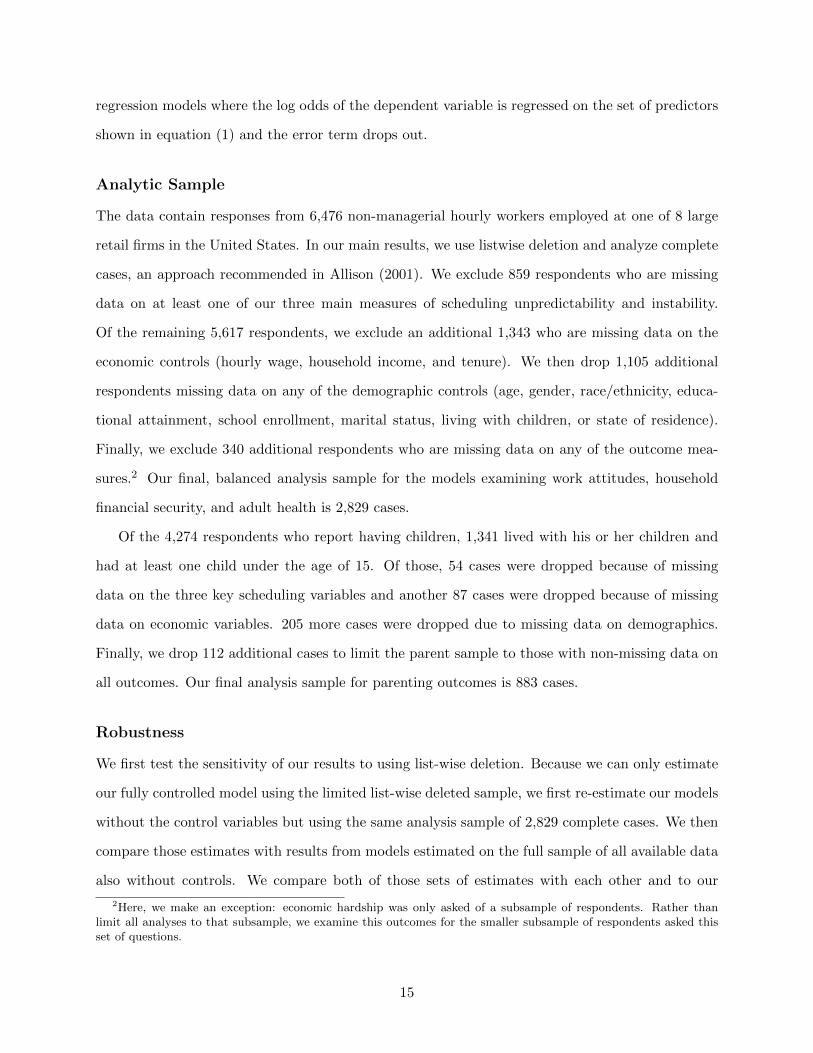
Analytic Sample

The data contain responses from 6,476 non-managerial hourly workers employed at one of 8 large

retail firms in the United States. In our main results, we use listwise deletion and analyze complete

cases, an approach recommended in Allison (2001). We exclude 859 respondents who are missing

data on at least one of our three main measures of scheduling unpredictability and instability.

Of the remaining 5,617 respondents, we exclude an additional 1,343 who are missing data on the

economic controls (hourly wage, household income, and tenure). We then drop 1,105 additional

respondents missing data on any of the demographic controls (age, gender, race/ethnicity, educa-

tional attainment, school enrollment, marital status, living with children, or state of residence).

Finally, we exclude 340 additional respondents who are missing data on any of the outcome mea-

sures.2 Our final, balanced analysis sample for the models examining work attitudes, household

financial security, and adult health is 2,829 cases.

Of the 4,274 respondents who report having children, 1,341 lived with his or her children and

had at least one child under the age of 15. Of those, 54 cases were dropped because of missing

data on the three key scheduling variables and another 87 cases were dropped because of missing

data on economic variables. 205 more cases were dropped due to missing data on demographics.

Finally, we drop 112 additional cases to limit the parent sample to those with non-missing data on

all outcomes. Our final analysis sample for parenting outcomes is 883 cases.

Robustness

We first test the sensitivity of our results to using list-wise deletion. Because we can only estimate

our fully controlled model using the limited list-wise deleted sample, we first re-estimate our models

without the control variables but using the same analysis sample of 2,829 complete cases. We then

compare those estimates with results from models estimated on the full sample of all available data

also without controls. We compare both of those sets of estimates with each other and to our

2Here, we make an exception: economic hardship was only asked of a subsample of respondents. Rather thanlimit all analyses to that subsample, we examine this outcomes for the smaller subsample of respondents asked thisset of questions.

15

preferred models.

In our main models, we present unweighted results for the regressions. To test robustness, we

re-estimate each of the regression models using the weights derived from ACS and CPS data. The

full details of the weighting procedures can be found in Appendix 1.

Third, we present the results of our analysis of the sensitivity of the estimates to unobserved

factors that could shape survey response and bias our estimates of the key relationships. Our gen-

eral approach is to define a dummy variable that represents one of a pair of opposing advertising

messages through which respondents were recruited. Then, we interact our key predictor vari-

ables with the dichotomous indicator for advertising message. In cases where we find consistent,

significant interactions, we show the implied upper and lower-bounds of our estimates.

Results

Descriptive Statistics

Scheduling Practices at Large Retailers

Table 2 describes the schedules of the retail workers in our main analytic sample. Schedule variabil-

ity and short-notice are common. The plurality of workers, 45%, report having variable schedules

with another 15% reporting a rotating shift. A smaller share, 21% has a regular day-time schedule,

while another 8% has a regular evening schedule and 9% has a regular night shift. Over all then,

less than a quarter work a regular standard time shift, another 15% work a regular non-standard

shift, and almost 60% work some kind of variable schedule.

Workers also receive little advance notice of their weekly schedules. 19% receive less than one

week of notice and 42% receive 1-2 weeks. A third receive their schedules between 2 and 3 weeks

out and a small minority, 7%, have at least three weeks notice. Together, 60% of workers have less

than two weeks of advance notice.

Finally, workers also experience substantial variation in the total hours they worked each week

over the month prior to interview. We calculate this measure as the amount of hours in the week in

which the respondent worked the most hours minus the amount of hours in the week the respondent

worked the fewest hours divided by the number of hours worked the week the respondent worked

the most hours. The mean percent variation is 33%, which implies that a worker that averaged

16

25 hours per week in the prior month likely worked as little as 20 hours at least one week of the

month and as many as 30 hours in another week during the same past month.

Attitudes, Financial Security, Health and Wellbeing, and Parenting

In Table 3 and Table 4, we present univariate statistics for our key outcomes, organized into the

domains of attitudes, household financial security, health and wellbeing, and parenting.

Workers in our sample express a clear desire for more hours (with 70% agreeing or strongly

agreeing that they would like more hours) and for more regular hours (with 86% agreeing or strongly

agreeing). By that measure, there is evidence that these unstable schedules are not preferable for

most workers, contrary to industry claims (Hatamiya, 2015).

There is also very low household financial security in our sample. Nearly half of workers report

that their household incomes vary from week-to-week, which is a striking level of income volatility.

One-third report that they have di�culty paying bills and meeting their expenses in a typical month

and respondents also report a mean of two economic hardships over the prior twelve months.

In Table 4, we show that nearly two-thirds of respondents report only good, fair, or poor health,

a third report “not being too happy,” three-quarters characterize their sleep quality as fair or poor,

and, perhaps most strikingly, 43% cross the threshold to serious psychological distress on the Kessler

6 scale.

Sample Inclusion and Weighting

The statistics described above characterize the un-weighted final analysis sample of 2,829 cases.

The second columns of statistics in Table 2, Table 3, and Table 4 describe the full set of the 6,632

non-managerial hourly employees we surveyed, some of whom are missing data on one or more

covariates. There are no notable di↵erences in these descriptive statistics between the two samples.

It does not appear that respondents who complete the entire survey instrument experience any

real di↵erences in scheduling as compared with respondents who skip items or do not complete the

survey.

Neither of these columns of statistics are, however, weighted to correct for bias in the demo-

graphics of our sample as compared to the known characteristics of workers in the industries and

occupations of interest. To adjust for such biases, we post-stratify our data by gender, age, and

17

race/ethnicity and re-weight our data to resemble the characteristics of workers in the industries

and occupations corresponding to our target sample frame as reflected in the American Commu-

nity Survey and the Current Population Survey. The full details of our weighting procedures are

described in the Appendix.

The third column of statistics in Table 2, Table 3, and Table 4 are estimated after weighting our

regression sample using weights constructed from the ACS. Column 4 weights the regression sample

instead using the Current Population Survey. In both cases, the distributions are very similar to

the unweighted means in columns 1 and 2.

Regression Results

We now turn to our estimates of the relationship between three key indicators of unpredictable and

unstable work schedules (week-to-week variability in hours worked, schedule type, and weeks of

advance notice) and four sets of outcome variables that capture: (1) work attitudes, (2) household

financial security, (3) worker health and wellbeing, and (4) parenting.

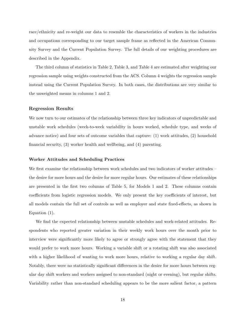
Worker Attitudes and Scheduling Practices

We first examine the relationship between work schedules and two indicators of worker attitudes –

the desire for more hours and the desire for more regular hours. Our estimates of these relationships

are presented in the first two columns of Table 5, for Models 1 and 2. These columns contain

coe�cients from logistic regression models. We only present the key coe�cients of interest, but

all models contain the full set of controls as well as employer and state fixed-e↵ects, as shown in

Equation (1).

We find the expected relationship between unstable schedules and work-related attitudes. Re-

spondents who reported greater variation in their weekly work hours over the month prior to

interview were significantly more likely to agree or strongly agree with the statement that they

would prefer to work more hours. Working a variable shift or a rotating shift was also associated

with a higher likelihood of wanting to work more hours, relative to working a regular day shift.

Notably, there were no statistically significant di↵erences in the desire for more hours between reg-

ular day shift workers and workers assigned to non-standard (night or evening), but regular shifts.

Variability rather than non-standard scheduling appears to be the more salient factor, a pattern

18

that holds across our models.

We see some similar patterns when we take desire to work more regular hours as the outcome.

There are strong and significant associations between working a variable or rotating schedule and

wanting more regular hours. Notably, these e↵ects are larger than the e↵ects on wanting more hours.

Taking predicted probabilities of each outcome by schedule type, we see that 72% of workers with

a variable shift and 74% of workers with a rotating shift wanted more hours compared with 66%

of regular day shift workers – about 10% more. But, 91% of workers with a variable shift and 92%

of workers with a rotating shift wanted more regular hours compared with 78% of regular day shift

workers – 15% more.

In contrast, advanced notice of work schedules was not related to either outcome.

Household Financial Security and Scheduling Practices

Unstable and unpredictable work schedules are negatively associated with household financial se-

curity, even after controlling for hourly wage, household income, and other control variables. The

relationships between work schedules and household financial security are shown in Models 3-5 of

Table 5.

The most pronounced e↵ects are on volatility in weekly household income. Recent week-to-week

variation in hours and working a variable or rotating (vs. stable day) schedule are all significantly

and positively related to reporting week-to-week income volatility. Having less than two weeks’

advance notice of one’s work schedule is also associated with income volatility. Compared to

having less than one week of advance notice, having 2-3 weeks or more than 3 weeks of advanced

notice significantly reduces the likelihood of experiencing income volatility. Interestingly, there is no

di↵erence between having less than 1 week and 1-2 weeks of advance notice. Having more advance

notice of one’s work schedule may make it easier for workers to maintain a second job, which could

help with income smoothing and reduce volatility.

The top panel of Figure 1 plots the predicted probability of experiencing income volatility by

recent week-to-week variation in hours, schedule type, and amount of advance notice. Approxi-

mately 34% of respondents who report very little variation in weekly hours report experiencing

income volatility. A significantly larger share, 47% of respondents with the median level of vari-

ation (30%) report volatility and 63% of respondents with variation at the 90th percentile report

19

income volatility. There are also large di↵erences by schedule type – with about 42% of workers

with regular shifts (day, evening, or night) reporting volatility compared with 53% of workers with

variable schedules and 49% of workers with rotating shifts. Similarly, while 53% of workers with

less than a week of advance notice and 50% of workers with 1-2 weeks of notice experience income

volatility, that share drops to 44% and 42% for workers with 2-3 weeks or more than 3 weeks of

notice, respectively.

Having a variable schedule also significantly increases the risk of having di�culty paying bills

and covering expenses and increases the number of household economic hardships. Though the

coe�cients are positively signed, there are not significant relationships between recent week-to-week

variation in hours and these outcomes. Advance notice is not associated with di�culty paying bills

but there is some evidence that greater advance notice (2-3 weeks) reduced reported hardships.

Worker Health and Wellbeing and Scheduling Practices

Unstable and unpredictable work schedules are also negatively associated with worker health and

wellbeing. Models 1-5 of Table 6 present the regression results for our measures of worker health

and wellbeing. With the exception of self-rated health, we find significant negative associations

between working a variable schedule (vs. a stable day schedule) and between having at least two

weeks of advance notice and our outcome measures. Those who work a variable schedule are less

likely to report being very or pretty happy or to report their sleep quality as very good or good.

They are more likely to score higher on the Kessler-6 measure of psychological distress and are

more likely to be in serious psychological distress.

It is notable that neither working a regular evening shift nor a regular night shift is significantly

associated with lower happiness or psychological distress. It is variability rather than non-standard

timing that seems to matter for these measures of wellbeing. The important exception here is

that working a regular night shift is significantly negatively associated with sleep quality and with

self-rated health.

Respondents who have at least two weeks notice are more likely to report being very or pretty

happy and more likely to report very good or good sleep quality. They also score lower on the

Kessler 6 and are less likely to cross the threshold to serious psychological distress. For each of

these outcomes, there is no significant di↵erence between having less than a week and 1-2 weeks

20

of notice. The meaningful threshold appears to be at 2 weeks of notice, with some evidence of

accumulating benefits of greater notice.

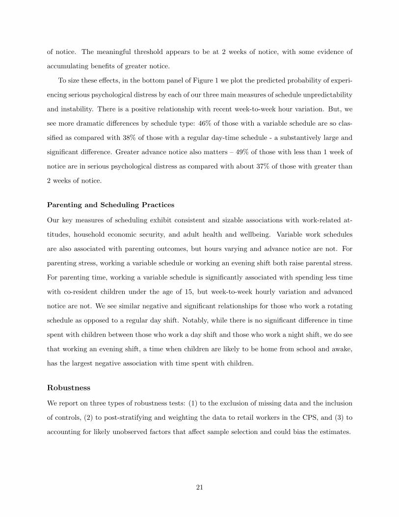
To size these e↵ects, in the bottom panel of Figure 1 we plot the predicted probability of experi-

encing serious psychological distress by each of our three main measures of schedule unpredictability

and instability. There is a positive relationship with recent week-to-week hour variation. But, we

see more dramatic di↵erences by schedule type: 46% of those with a variable schedule are so clas-

sified as compared with 38% of those with a regular day-time schedule - a substantively large and

significant di↵erence. Greater advance notice also matters – 49% of those with less than 1 week of

notice are in serious psychological distress as compared with about 37% of those with greater than

2 weeks of notice.

Parenting and Scheduling Practices

Our key measures of scheduling exhibit consistent and sizable associations with work-related at-

titudes, household economic security, and adult health and wellbeing. Variable work schedules

are also associated with parenting outcomes, but hours varying and advance notice are not. For

parenting stress, working a variable schedule or working an evening shift both raise parental stress.

For parenting time, working a variable schedule is significantly associated with spending less time

with co-resident children under the age of 15, but week-to-week hourly variation and advanced

notice are not. We see similar negative and significant relationships for those who work a rotating

schedule as opposed to a regular day shift. Notably, while there is no significant di↵erence in time

spent with children between those who work a day shift and those who work a night shift, we do see

that working an evening shift, a time when children are likely to be home from school and awake,

has the largest negative association with time spent with children.

Robustness

We report on three types of robustness tests: (1) to the exclusion of missing data and the inclusion

of controls, (2) to post-stratifying and weighting the data to retail workers in the CPS, and (3) to

accounting for likely unobserved factors that a↵ect sample selection and could bias the estimates.

21

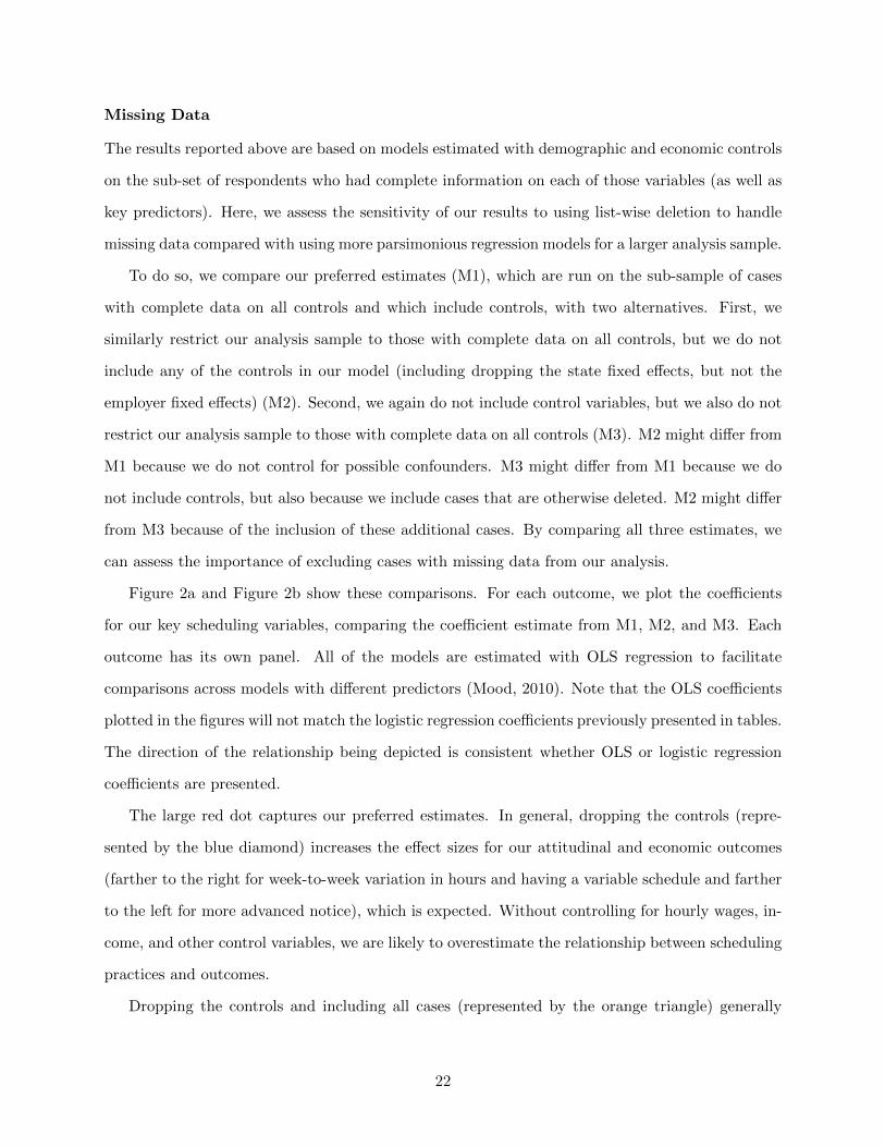
Missing Data

The results reported above are based on models estimated with demographic and economic controls

on the sub-set of respondents who had complete information on each of those variables (as well as

key predictors). Here, we assess the sensitivity of our results to using list-wise deletion to handle

missing data compared with using more parsimonious regression models for a larger analysis sample.

To do so, we compare our preferred estimates (M1), which are run on the sub-sample of cases

with complete data on all controls and which include controls, with two alternatives. First, we

similarly restrict our analysis sample to those with complete data on all controls, but we do not

include any of the controls in our model (including dropping the state fixed e↵ects, but not the

employer fixed e↵ects) (M2). Second, we again do not include control variables, but we also do not

restrict our analysis sample to those with complete data on all controls (M3). M2 might di↵er from

M1 because we do not control for possible confounders. M3 might di↵er from M1 because we do

not include controls, but also because we include cases that are otherwise deleted. M2 might di↵er

from M3 because of the inclusion of these additional cases. By comparing all three estimates, we

can assess the importance of excluding cases with missing data from our analysis.

Figure 2a and Figure 2b show these comparisons. For each outcome, we plot the coe�cients

for our key scheduling variables, comparing the coe�cient estimate from M1, M2, and M3. Each

outcome has its own panel. All of the models are estimated with OLS regression to facilitate

comparisons across models with di↵erent predictors (Mood, 2010). Note that the OLS coe�cients

plotted in the figures will not match the logistic regression coe�cients previously presented in tables.

The direction of the relationship being depicted is consistent whether OLS or logistic regression

coe�cients are presented.

The large red dot captures our preferred estimates. In general, dropping the controls (repre-

sented by the blue diamond) increases the e↵ect sizes for our attitudinal and economic outcomes

(farther to the right for week-to-week variation in hours and having a variable schedule and farther

to the left for more advanced notice), which is expected. Without controlling for hourly wages, in-

come, and other control variables, we are likely to overestimate the relationship between scheduling

practices and outcomes.

Dropping the controls and including all cases (represented by the orange triangle) generally

22

produces estimates that are either as large or larger than either of the two alternatives (though not

without exception).

Our preferred estimates for self-rated health are not significant and so we do not remark on

variation in those e↵ects. For happiness, sleep-quality, and psychological distress, the patterns are

generally similar to those for the attitudinal and economic outcomes – the coe�cients are as large

or larger without controls and without controls and with all cases as in the preferred models. This

robustness test suggests that omitted cases are unlikely to bias our estimates upward and imply

that some of our estimates of the relationships between scheduling practices and outcomes may be

conservative.

Weighted Results

The regression results above are estimated on unweighted data. We can also re-estimate the key

models with weights to adjust the sample demographics (age, race, and gender) to resemble the tar-

get population’s characteristics as tabulated from the American Community Survey or the Current

Population Survey.

Table 7 presents an alternative set of regression estimates that use the weights derived from

the American Community Survey. When weights are applied, the overrepresentation of women and

non-Hispanic whites in our sample is adjusted for. In general, there are few di↵erences between the

weighted and unweighted regression results.

For the two attitudinal outcomes, the results are similar. The relationship between week-to-

week hour variability and desiring more hours remains significant and is slightly stronger. However,

having a variable or rotating (vs. regular day) is no longer significantly associated with preferring

more work hours. Working a variable or rotating schedule remains significantly associated with

preferring more regular hours, though the coe�cients are about 30% smaller in size.

For the economic outcomes – income volatility, di�culty paying bills, and economic hardship

– the results are largely unchanged after weighting. Week-to-week variability in hours remains

significantly positively associated with income volatility, working a variable schedule is significantly

positively associated with all three measures, and working a rotating schedule significantly increases

the risk of income volatility and hardship. Having at least two weeks of advance notice of schedules

is, as before, significantly associated with lower levels of income volatility.

23

In the unweighted models of worker health and wellbeing, we did not find any significant as-

sociations with self-rated health, but for working the night shift. In Table 7, we see that after

weighting, this remains true. For happiness, the associations with scheduling practices reported

in Table 6 remain or are strengthened after weighting. For sleep quality, weighting attenuates the

relationship with having a variable schedule, but the beneficial e↵ect of greater advance notice

remains. Greater week-to-week variation in hours, having a variable or rotating schedule, and hav-

ing less than two weeks of advance notice are all still negatively and significantly associated with

psychological distress and with serious psychological distress.

Finally, the relationship between schedule type and both parenting stress and time remains

largely unchanged, with working a variable schedule or an evening shift associated with more

parental stress and less parental time with children.

These results are substantively unchanged if we use the weights derived from the Current

Population Survey rather than the American Community Survey.

Bounding the E↵ect of Sample Selection on Potentially Confounding Unobservables

The weighted results above give us confidence that any demographic biases in our sample compo-

sition in terms of age, gender, and race/ethnicity are not skewing our estimates of the relationship

between unstable and unpredictable scheduling practices and worker and family health and well-

being. However, it remains possible that workers select into our survey sample on the basis of

some unobserved characteristic and that same characteristic confounds the relationship between

scheduling practices and worker health and wellbeing.

We cannot definitively rule out the possibility that this sort of selection on a confounder is

occurring. But, we propose and test a method for assessing the presence of a specified confounder.

To do so, we first chose one such likely confounder – time pressure. Here, it is certainly possible

that workers who feel that they are time constrained would both be less likely to take our survey

and that time constraint could also bias the relationship between scheduling practices and health

and wellbeing.

We next developed a pair of advertising recruitment messages designed to elicit responses by

workers who were either “high” or “low” on this “unobserved” factor. For time pressure, we one

of two advertising messages to recruit respondents: either “Not getting enough hours at [EM-

24

PLOYER]?” or “Overworked at [EMPLOYER]?”

We then compare respondents recruited to the survey through each message channel. We first

conduct a manipulation check to determine if the messages actually serve to elicit responses from

di↵erent groups of potential respondents. For time-pressure, we compare respondents recruited

through the over-work message versus the insu�cient hours message in terms of their stated desire

for more work hours. There is a large and significant di↵erence between the two groups with 84% of

those who were recruited through the insu�cient hours message channel desiring more work hours

versus 68% of those who were recruited through the over-work message channel.

We next re-estimate each of our preferred models, now including an interaction between re-

cruitment message and each of our three key predictors – week-to-week hour variability, schedule

type, and weeks of advanced notice. If the unobserved variable “time pressure” confounds our key

relationships between scheduling practices and health and wellbeing, then we would expect that

the interaction terms would be significant. Of the 96 interaction terms across the twelve models,

only 7 were significant at the p <0.05 threshold. By chance, we would expect about 5 significant

coe�cients across 96 models.

Figure 3a and Figure 3b chart the predicted values of each outcome by predictor x message. In

these figures, each mini-figure plots the predicted values based on the interaction of a particular

predictor and message. There are then three mini-figures for each outcome (week-to-week variability

in hours, schedule type, and weeks of notice). In almost all cases, the 90% CI are overlapping,

indicating no di↵erence in the relationship by message type. The one interesting exception is

the desire for more hours. There, the relationship between unstable and unpredictable schedules

and desiring more hours is significantly weaker for those who are recruited through the over-work

channel versus the insu�cient hours channel.

Discussion

The Retail Work and Family Life Study collected data from a national sample of hourly retail

workers at eight large employers. We used a novel method of data collection, in which respondents

were recruited via targeted advertisements on Facebook. Using this approach, we address the

lack of data on scheduling practices available alongside data on economic, health, and wellbeing

outcomes. Our focus on a large sample of hourly retail workers is purposeful, allowing us to limit

25

sample heterogeneity on extraneous and potentially confounding variables such as socioeconomic

status and human capital and to examine a segment of the labor force acutely a↵ected by unstable

and unpredictable work schedules.

We focus on three scheduling practices that are expected to have negative e↵ects on workers and

their families: total work hours that vary from week to week, work schedules that vary, and short

advance notice of work schedules. Using our novel data, we estimated the associations between

each of these scheduling practices and economic, health and wellbeing, and parenting outcomes.

By and large, we find evidence that these scheduling practices have a range of negative e↵ects on

workers and their families. These types of associations have been reported in journalistic accounts

(Kantor, 2014; Singal, 2015) and in case studies (Haley-Lock, 2011; Henly and Lambert, 2014a),

and are consistent with findings on broader low and moderate income samples (Federal Reserve,

2014; Golden, 2015). We build upon this prior research and provide systematic evidence that these

practices are indeed associated with a range of negative outcomes for hourly workers employed in

the retail sector. Jobs in the retail sector are characterized not only by unpredictable and unstable

schedules, but also by low wages. Yet, even after adjusting for wages, incomes, and a range of other

control variables, unstable and unpredictable scheduling practices were still related to financial

insecurity, worse health outcomes, and parenting stress and reduced time with children for working

parents.

Because we rely on a non-probability sample, we are attentive to issues of potential sample

selectivity. We address selection issues in two ways. First, using post-stratification weighting, we

adjust the demographic characteristics of our sample to reflect the broader national population of

retail workers in the Current Population Survey and American Community Survey. Such post-

stratification weighting approaches have been shown to successfully address selectivity in samples

far more skewed than our own (Wang et al., 2015). This weighting procedure does not address po-

tential selectivity on unobserved characteristics, which we instead attempt to assess using targeted

advertisements with intentionally polarized recruitment messages, designed to attract workers on

both ends of a continuum with respect to potential confounding characteristics. Using this strategy,

we show that workers recruited by a message about “too many work hours” versus “insu�cient

work hours” yield a similar pattern of results with respect to the relationship between work sched-

ules and wellbeing outcomes. Our test of polarized recruitment messages provides some reassurance

26

that sample selectivity does not threaten our results.

Although our data provide novel evidence on how work scheduling practices a↵ect workers and

their families, some limitations and cautions should be kept in mind. Our analyses are cross-

sectional, and unobserved characteristics of individuals could lead some workers to sort into jobs

with particular scheduling practices or to be subject to certain scheduling practices within jobs and

to experience worse outcomes for reasons unrelated to those scheduling practices. We also cannot

eliminate the possibility of a reverse causal relationship between scheduling practices and worse

outcomes. Certainly, more research on how scheduling practices a↵ect workers and their families

would be desirable. While we have taken steps to guard against sample selectivity, particularly on

potentially confounding variables, future work should investigate other possible sources of sample

selection and seek to weight the data against employer-specific benchmarks.

Our research comes against the backdrop of a rapidly changing policy landscape, San Francisco

has recently implemented legislation that requires chain stores to provide two weeks of advance

notice of work schedules and access to more work hours, and several large cities including Seattle,

Washington D.C., and San Jose are considering similar legislation. Our research provides support

for the notion that requiring two weeks of advance notice would improve the lives of retail workers,

specifically, improving workers’ happiness, mental health, and economic security. Advance notice

of at least two weeks seems likely to improve workers’ ability to plan their child care, to combine

work with schooling or a second job, and in turn may reduce stress and improve mental health.

Our study also documents a robust and widespread relationships between variable work sched-

ules and economic, health, and parenting outcomes. Notably, local scheduling legislation does not

directly prohibit variable work schedules, but rather requires advance notice and access to full-time

hours before additional part-time workers are hired. These levers may well reduce variable work

schedules by providing workers with the ability to plan ahead and reduce variability via voluntary

shift trades, by reducing employer incentives to make last-minute schedule changes, and by pro-

viding workers with a greater number of expected hours. Still, whether these legislative changes, if

approved and implemented, will reduce variable work schedules remains to be seen. New, targeted

data collection will be necessary to answer this question.

The imminent changes in scheduling law and company practice provide an opportunity to study

the e↵ects of an exogenous change in work scheduling practices. Future research, capitalizing on

27

these exogenous changes, would represent an important step forward in understanding the causal

link between work schedule practices and financial security, health, and wellbeing of workers and

their families. Although our results are not definitive, they add to a growing body of evidence that

scheduling practices have substantial e↵ects on the lives of workers and their families and that an

increase in the stability and predictability of work schedules would be likely to have a range of

beneficial e↵ects.

28

References

Ala-Mursula L., Vahtera J., Kivimaki M., Kevin M.V., Pentti J. 2002. “Employee control overworking times: associations with subjective health and sickness absences.” Journal of Epi-demiology and Community Health 56(4): 272-278.

Allison, P.D. 2001. Missing Data: Series: Quantitative Applications in the Social Sciences. SagePublications.

Appelbaum, E., A. Bernhardt, and R.J. Murnane. (Eds.). 2003. Low-Wage America: How Em-ployers are Reshaping Opportunity in the Workplace. New York: Russell Sage Foundation.

Ben-Ishai, L. 2015a. “Federal Legislation to Address Volatile Job Schedules” CLASP ResearchBrief.

Ben-Ishai, L. 2015b. “Volatile Job Schedules and Access to Public Benefits” CLASP ResearchBrief.

Ben-Ishai, L., H. Matthews, and J. Levin-Epstein. 2014. Scrambling for Stability: The Challengesof Job Schedule Volatility and Child Care. Washington, DC: Center for Law and Social Policy.

Bhutta, C.B.. 2012. “Not by the Book: Facebook as a Sampling Frame.” Sociological Methods &Research 41(1): 57-88.

Clawson, D., and N. Gerstel. 2015. Unequal Time: Gender, Class, and Family in EmploymentSchedules. New York: Russell Sage Foundation.

Davis K.D., Lawson K.M., Almeida D.M., Davis K.D., King R.B., Hammer L.B., Casper L.,Okechukwu C.A., Hanson G.C., McHale S.M. 2015. “Parent’s Daily Time with Their Children:A Workplace Intervention.” Pediatrics.

Enchautegui, M. E., M. Johnson, and J. Gelatt. 2015. “Who Minds the Kids When Mom Worksa Nonstandard Schedule?” Urban Institute.

Federal Reserve Bank Board of Governors. 2014. Report on the Economic Well-Being of U.S.Households in 2013.

Fligstein, N. and T.J. Shin. 2004. “The Shareholder Value Society: A Review of the Changes inWorking Conditions and Inequality in the United States, 1976 to 2000.” In Social Inequality.Ed. Katherine Neckerman. New York: Russell Sage Foundation Press.

Flood, S., M. King, S. Ruggles, and J.R. Warren. Integrated Public Use Microdata Series, Cur-rent Population Survey: Version 4.0. [Machine-readable database]. Minneapolis: University ofMinnesota, 2015.

Gassman-Pines, A. 2013. “Daily Spillover of Low-Income Mothers’ Perceived Workload to Moodand Mother-Child Interactions.” Journal of Marriage and Family 75(5):1304-1318.

Gennetian, L. A., S. Wolf, H.D. Hill, and P. Morris. 2015. “Intrayear Household Income Dynamicsand Adolescent School Behavior.” Demography 52(2):455-483.

Goel, S., Rao, J. M., and Shro↵, R. 2015. Precinct or Prejudice? Understanding Racial Disparitiesin New York City’s Stop-and-Frisk Policy. The Annals of Applied Statistics. 10(1):365-394.

29

Goh, J., Pfe↵er, J., and Zenios, S. 2015. “Exposure to Harmful Workplace Practices Could Accountfor Inequality in Life Spans Across Di↵erent Demographic Groups.” Health A↵airs 34(10):1761-1768.

Golden, L. 2001. “Flexible Work Schedules: What Are We Trading O↵ to Get Them¿‘ MonthlyLabor Review 124(3): 50-67.

Golden, L. 2015. “Irregular Work Scheduling and Its Consequences.” BriefingPaper #394. Economic Policy Institute. http://www.epi.org/publication/

irregular-work-scheduling-and-its-consequences

Hacker, J. 2006. The Great Risk Shift: The New Economic Insecurity and the Decline of theAmerican Dream. Oxford University Press.

Haley-Lock, A. 2011. “Place-Bound Jobs at the Intersection of Policy and Management: Com-paring Employer Practices in US and Canadian Chain Restaurants.” American BehavioralScientist 55(7): 823-842

Halliday, T.J. 2007. “Income Volatility and Health.” IZA Discussion Paper.

Han, W. 2005. “Maternal Nonstandard Work Schedules and Child Cognitive Outcomes.” ChildDevelopment 76(1): 137-154.

Harris MM, Fennell ML. 1988. “A multivariate model of job stress and alcohol consumption.”Sociological Quarterly 29(3): 391-406

Hatamiya, L. 2015. A Practical Analysis of San Francisco’s Predictive Scheduling and Fair Treat-ment for Formula Retail Employees Ordinance. Report prepared for the California RetailersAssociation.

Henly, J.R., H.L. Shaefer, and E. Waxman. 2006. “Nonstandard Work Schedules: Employer- andEmployee-Driven Flexibility in Retail Jobs.” Social Service Review 80: 609-34.

Henly, J. R., and S. Lambert. 2005. “Nonstandard Work and Child-Care Needs of Low-IncomeParents.” In S.M. Bianchi, L.M. Casper, and B.R. King (Ed) Work, Family, Health, andWell-Being (pp. 473-492). Mahwah, NJ, US: Lawrence Erlbaum Associates Publishers.

Henly, J. R., and Lambert, S. J. 2014a. “Unpredictable Work Timing in Retail Jobs Implicationsfor Employee Work-Life Conflict.” Industrial & Labor Relations Review 67(3): 986-1016.

Henly, J. R., and Lambert, S. J. 2014b. Measuring Precarious Work Schedules. University ofChicago. EINet Working Paper.

Henly, J.R., H.L. Shaefer, and E. Waxman. 2006. “Nonstandard Work Schedules: Employer- andEmployee-Driven Flexibility in Retail Jobs.” Social Service Review 80(4): 609-634.

Houseman, S. 2001. “Why Employers Use Flexible Sta�ng Arrangements: Evidence from anEstablishment Survey.” Industrial and Labor Relations Review 55(1): 149-170.

Hurtado, D. A., Okechukwu, C. A., Buxton, O. M., Hammer, L., Hanson, G. C., Moen, P.,Klein, L.C., and Berkman, L. F. 2016. “E↵ects on Cigarette Consumption of a Work-FamilySupportive Organizational Intervention: 6-month Results from the Work, Family and HealthNetwork Study.” Journal of Epidemiology and Community Health.

30

Joshi, P. and K. Bogen. 2007. “Nonstandard Schedules and Young Children’s Behavioral OutcomesAmong Working Low-Income Families.” Journal of Marriage and Family 69(1):139-156.

Kalleberg, A. L. 2009. “Precarious Work, Insecure Workers: Employment Relations in Transition.”American Sociological Review 74(1):1-22.

Kalleberg, A. 2013. Good Jobs, Bad Jobs: The Rise of Polarized and Precarious EmploymentSystems in the United States, 1970s to 2000s. New York: Russell Sage Foundation.

Kantor, J. 2014. “Working Anything but 9 to 5.” The New York Times. August 13.

Kessler, R. et al. 2003. “Screening for Serious Mental Illness in the General Population.” JAMAPsychiatry 60(2): 184-189.

Kouvonen A, Kivimki M, Virtanen M, Pentti J, Vahtera J. 2005. “Work Stress, Smoking Status,and Smoking Intensity: An Observational Study of 46,190 Employees.” J. Epidemiology andCommunity Health 59(1):63-69.

Lambert, S.J., P. Fugiel, and J.R. Henly. 2014. Precarious Work Schedules among Early-CareerEmployees in the US: A National Snapshot. University of Chicago.

Leete, L. and N. Bania. 2010. “The E↵ect of Income shocks on Food Insu�ciency.“ Review ofEconomics of the Household 8(4): 505-526.

Link, B.G and J. Phelan. 1995. “Social Conditions As Fundamental Causes of Disease.” Journalof Health and Social Behavior 35: 80-94.

Luce, S., S. Hammond, and D. Sipe. 2014. Short Shifted. Retail Action Project and CUNY.

Marmot, M.G, H. Bosma, H. Hemingway, E. Brunner, S. Stansfeld. 1997. “Contribution of JobControl and Other Risk Factors to Social Variations in Coronary Heart Disease Incidence.”Lancet 350: 235-239.

McMenamin, T. 2007. “A Time to Work: Recent Trends in Shift Work and Flexible Schedules.”Monthly Labor Review 130: 3-15.

Miller, D.P., and W. Han. 2008. “Maternal Nonstandard Work Schedules and Adolescent Over-weight.” American Journal of Public Health 98(8): 1495-1502.

Moen P, Kelly EL, Lee S-R, Almeida DM, Kossek EE, Buxton OM. 2016. “Does a Fleixibility/-Support Organizational Initiative Improve High-Tech Employees’ Well-Being? Evidence fromthe Work, Family, and Health Network.” American Sociological Review 81(1):134-164.

Morsy, L., and R. Rothstein. 2015. “Parents’ Non-Standard Work Schedules Make Adequate Chil-drearing Di�cult.” Economic Policy Institute. Washington D.C.

Mullinix, K.J., T.J. Leeper, J.N. Druckman, and J. Freese. Forthcoming. “The Generalizability ofSurvey Experiments.“ Journal of Experimental Political Science.

Murdoch, J. and R. Schneider. 2014. “Spikes and Dips: How Income Uncertainty A↵ects House-holds.” U.S. Financial Diaries. December 4,

Olson R, Crain TL, Bodner T, King RB, Hammer LB, Klein LC, Erikson L, Moen P, Berkman LF,Buxton OM. 2015. “A Workplace Intervention Improves Sleep: Results from the RandomizedControlled Work, Family & Health Study.” Sleep Health 1(1):55-65

31

Perrin, A. 2015. “Social Networking Usage: 2005-2015.” Pew Research Center.

Presser, H. B. 2003. Working in a 24/7 Economy. New York: Russell Sage Foundation.

Presser, H.B. 1999. “Toward a 24-hour Economy.“ Science 284.5421:1778-1779.

Ruggles, S., K. Genadek, R. Goeken, J. Grover, and M. Sobek. Integrated Public Use MicrodataSeries: Version 6.0 [Machine-readable database]. Minneapolis: University of Minnesota, 2015.

Schneider, W., J. Brooks-Gunn, J. Waldfogel. 2013. “The Great Recession and the Risk for ChildMaltreatment.” Child Abuse & Neglect 37(10): 721-729.

Scott, E. K., K. Edin, A.S. London, and R.J. Kissane. 2004. “Unstable Work, Unstable Income:Implications for Family Wellbeing in the Era of Time-Limited Welfare.” Journal of Poverty8(1): 61-88.

Singal, J. 2015. “How Parents’ Unpredictable Work Schedules Harm Kids.” New York Magazine.August 14.

Strauss, V. 2015. “The Consequences for Kids when Parents Work Irregular Night Shifts - Re-search.” The Washington Post. August 9.

Wang, W., Rothschild, D., Goel, S., and Gelman, A. 2015. “Forecasting elections with non-representative polls.” International Journal of Forecasting 31(3): 980-991.

White, G.B. 2015. “The Very Real Hardship of Unpredictable Work Schedules.” The Atlantic.April 15.

Wight, V.R., S.B. Raley, and S.M. Bianchi. 2008. “Time for Children, One’s Spouse and Oneselfamong Parents Who Work Nonstandard Hours.” Social Forces 87(1): 243-271.

Williams, J. C., and H. Boushey. 2010. “The Three Faces of Work-Family Conflict: The Poor,the Professionals, and the Missing Middle.” AvailableSSRN::http://ssrn.com/abstract=

2126314

Wolf, S., L.A. Gennetian, P.A. Morris, and H.D. Hill. 2014. “Patterns of Instability among Low-and Middle-Income Households with Children.” Family Relations 63(3): 397-410.

Zeytinoglu, I., W. Lillevik, M. Seaton, J. Moruz. 2004. “Part-Time and Casual Work in RetailTrade: Stress and Other Factors A↵ecting the Workplace.” Relations Industrielles 59(3): 516-542.

32

Tables

Table 1: Comparison of Demographics of Unweighted and Weighted Survey Data with Character-istics of ACS and CPS Samples

(1) (2) (3) (4) (5)Analysis Sample Analysis Sample Analysis Sample ACS Sample CPS Sample

Unweighted ACS Weights CPS Weights

GenderMale 24% 44% 44% 44% 44%Female 76% 56% 56% 56% 56%

Age18-19 13% 14% 12% 14% 12%20-29 42% 38% 38% 38% 38%30-39 22% 18% 20% 17% 20%40-49 20% 18% 19% 18% 19%50+ 4% 12% 10% 13% 11%

Race/EthnicityWhite, Non-Hispanic 75% 64% 57% 63% 55%Black, Non-Hispanic 6% 11% 13% 12% 14%Hispanic 12% 16% 21% 16% 21%Other or Two or More 7% 8% 9% 8% 9%Races, Non-Hispanic

Educational AttainmentHigh School or Less 42% 44% 44% 62% 56%Some College (including AA) 50% 48% 47% 29% 35%BA or more 8% 8% 9% 8% 9%

Enrolled in School 25% 26% 25% 26% 27%

N 2829 2829 2829 154451 10527

33

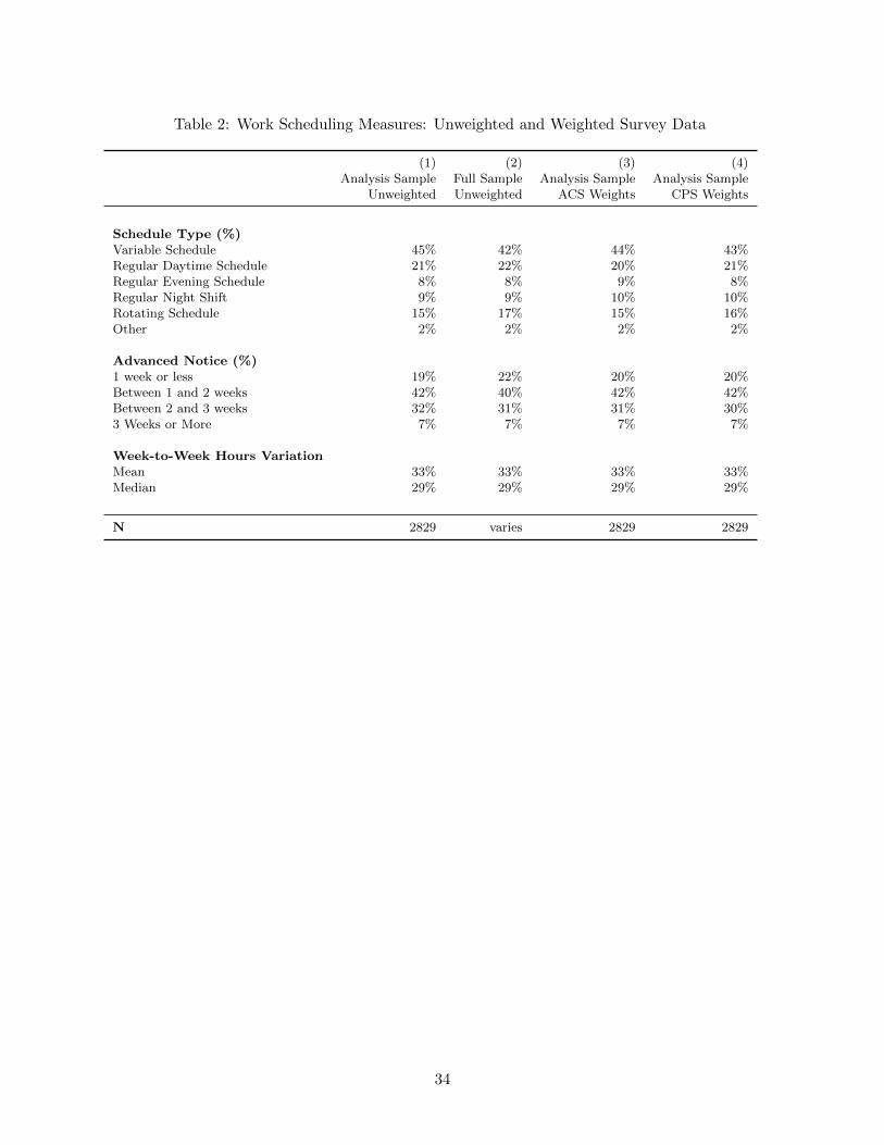
Table 2: Work Scheduling Measures: Unweighted and Weighted Survey Data

(1) (2) (3) (4)Analysis Sample Full Sample Analysis Sample Analysis Sample

Unweighted Unweighted ACS Weights CPS Weights

Schedule Type (%)Variable Schedule 45% 42% 44% 43%Regular Daytime Schedule 21% 22% 20% 21%Regular Evening Schedule 8% 8% 9% 8%Regular Night Shift 9% 9% 10% 10%Rotating Schedule 15% 17% 15% 16%Other 2% 2% 2% 2%

Advanced Notice (%)1 week or less 19% 22% 20% 20%Between 1 and 2 weeks 42% 40% 42% 42%Between 2 and 3 weeks 32% 31% 31% 30%3 Weeks or More 7% 7% 7% 7%

Week-to-Week Hours VariationMean 33% 33% 33% 33%Median 29% 29% 29% 29%

N 2829 varies 2829 2829

34

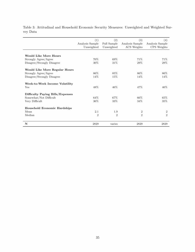
Table 3: Attitudinal and Household Economic Security Measures: Unweighted and Weighted Sur-vey Data

(1) (2) (3) (4)Analysis Sample Full Sample Analysis Sample Analysis Sample

Unweighted Unweighted ACS Weights CPS Weights

Would Like More HoursStrongly Agree/Agree 70% 69% 71% 71%Disagree/Strongly Disagree 30% 31% 29% 29%

Would Like More Regular HoursStrongly Agree/Agree 86% 85% 86% 86%Disagree/Strongly Disagree 14% 15% 14% 14%

Week-to-Week Income VolatilityYes 48% 46% 47% 46%

Di�culty Paying Bills/ExpensesSomewhat/Not Di�cult 64% 67% 66% 65%Very Di�cult 36% 33% 34% 35%

Household Economic HardshipsMean 2.1 1.9 2 2Median 2 2 2 2

N 2829 varies 2829 2829

35

Table 4: Health and Parenting Measures: Unweighted and Weighted Survey Data

(1) (2) (3) (4)Analysis Sample Full Sample Analysis Sample Analysis Sample

Unweighted Unweighted ACS Weights CPS Weights

Self Rated HealthExcellent/Very Good 33% 34% 36% 36%Good/Fair/Poor 67% 66% 64% 64%

HappinessVery/Pretty Happy 67% 68% 67% 67%Not too Happy 33% 32% 33% 33%

Sleep QualityVery Good/Good 24% 25% 26% 26%Fair/Poor 76% 75% 74% 74%

Serious Psychological DistressYes 43% 41% 42% 42%

Psychological Distress ScoreMean 11.5 11.3 11.4 11.3Median 12 11 11 11

Parenting Stress ScoreMean 5.1 5 5 5Median 5 5 5 5

Parenting Time ScoreMean 11.9 12 11.8 11.8Median 12 12 12 12

N 2829 varies 2829 2829

36

Table 5: Relationship between Work Scheduling Experiences and Worker Attitudes/HouseholdEconomic Security

(1) (2) (3) (4) (5)Prefer More Prefer More Income Di�culty # of

Hours Regular Hours Volatile Paying Bills Hardships

Recent Weekly Hour Variation 0.772⇤⇤ 0.361 1.950⇤⇤⇤ 0.227 0.284

Work Schedule TypeRegular Day Shift (ref) (ref) (ref) (ref) (ref)Variable Shift 0.267⇤ 1.028⇤⇤⇤ 0.532⇤⇤⇤ 0.302⇤ 0.525⇤⇤⇤

Regular Evening Shift -0.122 -0.165 0.056 0.234 -0.001Regular Night Shift -0.051 -0.382⇤ -0.074 0.087 0.372Rotating Schedule 0.398⇤ 1.090⇤⇤⇤ 0.359⇤ 0.184 0.349⇤

Other Schedule -0.221 0.227 -0.233 0.346 0.373

Week of Advanced NoticeLess than 1 Week (ref) (ref) (ref) (ref) (ref)Between 1 and 2 Weeks 0.225 -0.013 -0.145 0.140 -0.153Between 2 and 3 Weeks 0.254 -0.219 -0.448⇤⇤ -0.006 -0.304⇤

3 Weeks or More 0.275 -0.388 -0.524⇤ -0.053 -0.164

N 2829 2829 2829 2829 1365⇤ p < .05, ⇤⇤ p < .01, ⇤⇤⇤ p < .001

All models include controls for race, age, gender, educational attainment, marital status, school enrollment, hourlywage, household income, average weekly work hours, employment tenure, and living with children as well as stateand employer fixed-e↵ects.

37

Table 6: Relationship between Work Scheduling Experiences and Worker Health and Wellbeing/Parenting

(1) (2) (3) (4) (5) (6) (7)Self-Rated Happiness Sleep Psychological Serious Parenting ParentingHealth Quality Distress Psych Distress Stress Time

Recent Weekly Hour Variation -0.155 -0.133 -0.281 1.529⇤⇤ 0.502⇤ 0.107 -0.872

Work Schedule TypeRegular Day Shift (ref) (ref) (ref) (ref) (ref) (ref) (ref)Variable Shift -0.176 -0.502⇤⇤⇤ -0.294⇤ 0.826⇤⇤ 0.360⇤⇤ 0.502⇤ 2.043⇤⇤⇤

Regular Evening Shift 0.102 0.253 0.053 -0.582 -0.171 1.205⇤⇤ 3.073⇤⇤⇤

Regular Night Shift -0.514⇤⇤ -0.206 -0.504⇤⇤ 0.482 0.201 0.421 0.678Rotating Schedule -0.116 -0.257 -0.281 0.444 0.210 -0.272 1.902⇤⇤

Other Schedule -0.347 -0.418 -0.168 -0.182 0.308 0.013 1.017

Week of Advanced NoticeLess than 1 Week (ref) (ref) (ref) (ref) (ref) (ref) (ref)Between 1 and 2 Weeks 0.168 0.100 0.187 -0.622 -0.170 0.257 0.641Between 2 and 3 Weeks 0.216 0.493⇤⇤ 0.344⇤ -1.536⇤⇤⇤ -0.535⇤⇤⇤ -0.0250 0.6783 Weeks or More 0.267 0.441⇤ 0.889⇤⇤⇤ -1.708⇤⇤ -0.517⇤ 0.184 -0.639

N 2829 2829 2829 2829 2829 883 883⇤ p < .05, ⇤⇤ p < .01, ⇤⇤⇤ p < .001

All models include controls for race, age, gender, educational attainment, marital status, school enrollment, hourly wage, household income, average weekly workhours, employment tenure, and living with children as well as state and employer fixed-e↵ects.

38

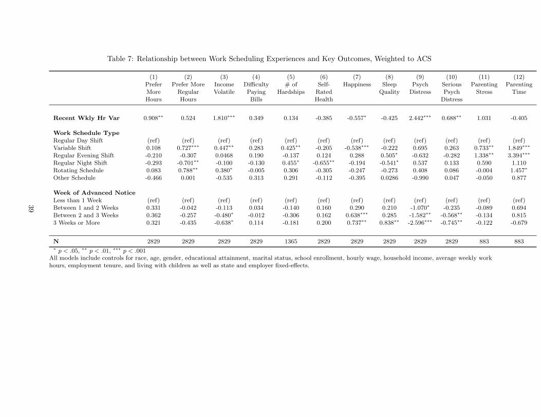
Table 7: Relationship between Work Scheduling Experiences and Key Outcomes, Weighted to ACS

(1) (2) (3) (4) (5) (6) (7) (8) (9) (10) (11) (12)Prefer Prefer More Income Di�culty # of Self- Happiness Sleep Psych Serious Parenting ParentingMore Regular Volatile Paying Hardships Rated Quality Distress Psych Stress TimeHours Hours Bills Health Distress

Recent Wkly Hr Var 0.908⇤⇤ 0.524 1.810⇤⇤⇤ 0.349 0.134 -0.385 -0.557⇤ -0.425 2.442⇤⇤⇤ 0.688⇤⇤ 1.031 -0.405

Work Schedule TypeRegular Day Shift (ref) (ref) (ref) (ref) (ref) (ref) (ref) (ref) (ref) (ref) (ref) (ref)Variable Shift 0.108 0.727⇤⇤⇤ 0.447⇤⇤ 0.283 0.425⇤⇤ -0.205 -0.538⇤⇤⇤ -0.222 0.695 0.263 0.733⇤⇤ 1.849⇤⇤⇤

Regular Evening Shift -0.210 -0.307 0.0468 0.190 -0.137 0.124 0.288 0.505⇤ -0.632 -0.282 1.338⇤⇤ 3.394⇤⇤⇤

Regular Night Shift -0.293 -0.701⇤⇤ -0.100 -0.130 0.455⇤ -0.655⇤⇤ -0.194 -0.541⇤ 0.537 0.133 0.590 1.110Rotating Schedule 0.083 0.788⇤⇤ 0.380⇤ -0.005 0.306 -0.305 -0.247 -0.273 0.408 0.086 -0.004 1.457⇤

Other Schedule -0.466 0.001 -0.535 0.313 0.291 -0.112 -0.395 0.0286 -0.990 0.047 -0.050 0.877

Week of Advanced NoticeLess than 1 Week (ref) (ref) (ref) (ref) (ref) (ref) (ref) (ref) (ref) (ref) (ref) (ref)Between 1 and 2 Weeks 0.331 -0.042 -0.113 0.034 -0.140 0.160 0.290 0.210 -1.070⇤ -0.235 -0.089 0.694Between 2 and 3 Weeks 0.362 -0.257 -0.480⇤ -0.012 -0.306 0.162 0.638⇤⇤⇤ 0.285 -1.582⇤⇤ -0.568⇤⇤ -0.134 0.8153 Weeks or More 0.321 -0.435 -0.638⇤ 0.114 -0.181 0.200 0.737⇤⇤ 0.838⇤⇤ -2.596⇤⇤⇤ -0.745⇤⇤ -0.122 -0.679

N 2829 2829 2829 2829 1365 2829 2829 2829 2829 2829 883 883⇤ p < .05, ⇤⇤ p < .01, ⇤⇤⇤ p < .001

All models include controls for race, age, gender, educational attainment, marital status, school enrollment, hourly wage, household income, average weekly workhours, employment tenure, and living with children as well as state and employer fixed-e↵ects.

39

Figures

Figure 1: Predicted Probability of Household Income Volatility (top 3) and of Serious Psychological Distress (bottom

3) by Scheduling Experiences

.2.3

.4.5

.6.7

Pr(E

xper

ienc

e W

eek

to W

eek

Inco

me

Vola

tility

)

0 .1 .2 .3 .4 .5 .6 .7

Variation in Weekly Hours

.25

.35

.45

.55

VariableReg. Day

Reg. Eve.Reg. Night

Rotating

Type of Work Schedule

.25

.35

.45

.55

< 1 Wk1-2 Wks

2-3 Wks>= 3 Wks

Weks of Usual Advance Notice

.2.3

.4.5

.6.7

Pr(E

xper

ienc

ing

Serio

us P

sych

olog

ical

Dis

tress

)

0 .1 .2 .3 .4 .5 .6 .7

Variation in Weekly Hours

.25

.35

.45

.55

VariableReg. Day

Reg. Eve.Reg. Night

Rotating

Type of Work Schedule

.25

.35

.45

.55

< 1 Wk1-2 Wks

2-3 Wks>= 3 Wks

Weeks of Usual Advance Notice

40

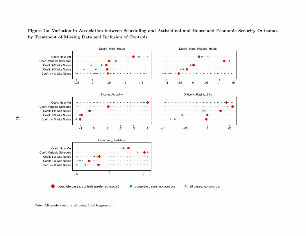
Figure 2a: Variation in Association between Scheduling and Attitudinal and Household Economic Security Outcomes

by Treatment of Missing Data and Inclusion of Controls

-.05 0 .05 .1 .15

Coeff: >= 3 Wks NoticeCoeff: 2-3 Wks NoticeCoeff: 1-2 Wks Notice

Coeff: Variable ScheduleCoeff: Hour Var

Desire_More_Hours

-.1 -.05 0 .05 .1 .15

Desire_More_Regular_Hours

-.1 0 .1 .2 .3 .4

Coeff: >= 3 Wks NoticeCoeff: 2-3 Wks NoticeCoeff: 1-2 Wks Notice

Coeff: Variable ScheduleCoeff: Hour Var

Income_Volatility

-.1 -.05 0 .05

Difficulty_Paying_Bills

-.5 0 .5

Coeff: >= 3 Wks NoticeCoeff: 2-3 Wks NoticeCoeff: 1-2 Wks Notice

Coeff: Variable ScheduleCoeff: Hour Var

Economic_Hardships

complete cases, controls (preferred model) complete cases, no controls all cases, no controls

Note: All models estimated using OLS Regression.

41

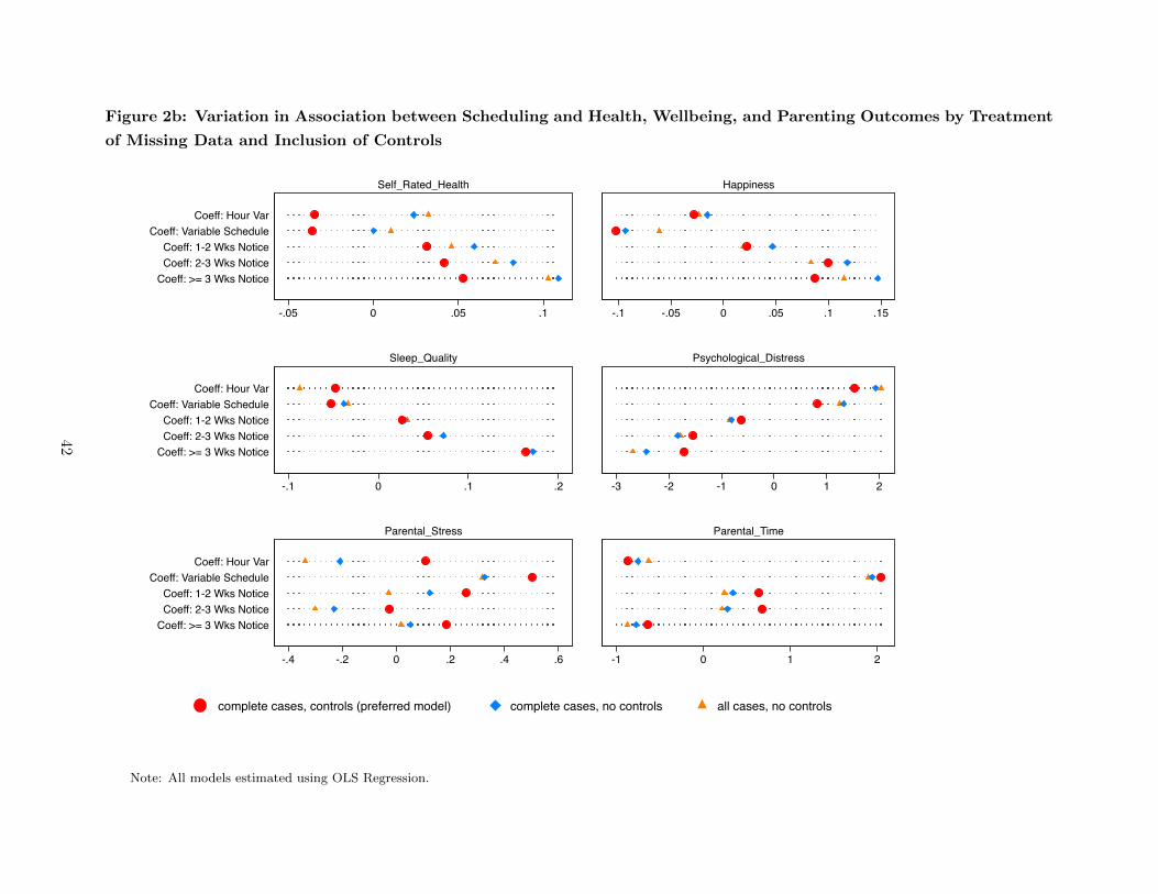
Figure 2b: Variation in Association between Scheduling and Health, Wellbeing, and Parenting Outcomes by Treatment

of Missing Data and Inclusion of Controls

-.05 0 .05 .1

Coeff: >= 3 Wks NoticeCoeff: 2-3 Wks NoticeCoeff: 1-2 Wks Notice

Coeff: Variable ScheduleCoeff: Hour Var

Self_Rated_Health

-.1 -.05 0 .05 .1 .15

Happiness

-.1 0 .1 .2

Coeff: >= 3 Wks NoticeCoeff: 2-3 Wks NoticeCoeff: 1-2 Wks Notice

Coeff: Variable ScheduleCoeff: Hour Var

Sleep_Quality

-3 -2 -1 0 1 2

Psychological_Distress

-.4 -.2 0 .2 .4 .6

Coeff: >= 3 Wks NoticeCoeff: 2-3 Wks NoticeCoeff: 1-2 Wks Notice

Coeff: Variable ScheduleCoeff: Hour Var

Parental_Stress

-1 0 1 2

Parental_Time

complete cases, controls (preferred model) complete cases, no controls all cases, no controls

Note: All models estimated using OLS Regression.

42

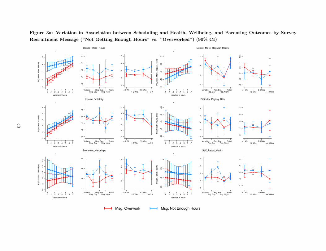
Figure 3a: Variation in Association between Scheduling and Health, Wellbeing, and Parenting Outcomes by Survey

Recruitment Message (“Not Getting Enough Hours” vs. “Overworked”) (90% CI).5

.6.7

.8.9

Pr(D

esire

_Mor

e_Ho

urs)

0 .1 .2 .3 .4 .5 .6 .7variation in hours

'

.6.7

.8.9

1

VariableReg. Day

Reg. Eve.Reg. Night

Rotating

.4.6

.81

1.2

< 1 Wk1-2 Wks

2-3 Wks>= 3 Wks

Desire_More_Hours

.8.8

5.9

.95

1

Pr(D

esire

_Mor

e_Re

gula

r_Ho

urs)

0 .1 .2 .3 .4 .5 .6 .7variation in hours

'

.7.8

.91

VariableReg. Day

Reg. Eve.Reg. Night

Rotating

.8.8

5.9

.95

11.

05

< 1 Wk1-2 Wks

2-3 Wks>= 3 Wks

Desire_More_Regular_Hours

.3.4

.5.6

.7.8

Pr(In

com

e_Vo

latili

ty)

0 .1 .2 .3 .4 .5 .6 .7variation in hours

'

0.2

.4.6

.8

VariableReg. Day

Reg. Eve.Reg. Night

Rotating

.2.3

.4.5

.6.7

< 1 Wk1-2 Wks

2-3 Wks>= 3 Wks

Income_Volatility

.35

.4.4

5.5

.55

Pr(D

ifficu

lty_P

ayin

g_Bi

lls)

0 .1 .2 .3 .4 .5 .6 .7variation in hours

'

.2.3

.4.5

.6

VariableReg. Day

Reg. Eve.Reg. Night

Rotating

.3.4

.5.6

.7

< 1 Wk1-2 Wks

2-3 Wks>= 3 Wks

Difficulty_Paying_Bills

1.8

22.

22.

42.

62.

8

Pr(E

cono

mic_

Hard

ship

s)

0 .1 .2 .3 .4 .5 .6 .7variation in hours

'

12

34

VariableReg. Day

Reg. Eve.Reg. Night

Rotating

11.

52

2.5

3

< 1 Wk1-2 Wks

2-3 Wks>= 3 Wks

Economic_Hardships

.25

.3.3

5.4

Pr(S

elf_

Rate

d_He

alth

)

0 .1 .2 .3 .4 .5 .6 .7variation in hours

'

0.2

.4.6

.8

Variable

Reg. DayReg. Eve.

Reg. NightRotating

.1.2

.3.4

.5

< 1 Wk1-2 Wks

2-3 Wks>= 3 Wks

Self_Rated_Health

Msg: Overwork Msg: Not Enough Hours

43

Figure 3b: Variation in Association between Scheduling and Health, Wellbeing, and Parenting Outcomes by Survey

Recruitment Message (“Not Getting Enough Hours” vs. “Overworked”) (90% CI).5

5.6

.65

.7

Pr(H

appi

ness

)

0 .1 .2 .3 .4 .5 .6 .7variation in hours

'

.4.6

.81

VariableReg. Day

Reg. Eve.Reg. Night

Rotating

.4.5

.6.7

.8

< 1 Wk1-2 Wks

2-3 Wks>= 3 Wks

Happiness

.15

.2.2

5.3

Pr(S

leep

_Qua

lity)

0 .1 .2 .3 .4 .5 .6 .7variation in hours

'

0.1

.2.3

.4

VariableReg. Day

Reg. Eve.Reg. Night

Rotating

.1.2

.3.4

.5

< 1 Wk1-2 Wks

2-3 Wks>= 3 Wks

Sleep_Quality

1011

1213

14

Pr(P

sych

olog

ical_

Dist

ress

)

0 .1 .2 .3 .4 .5 .6 .7variation in hours

'

810

1214

VariableReg. Day

Reg. Eve.Reg. Night

Rotating

1011

1213

14

< 1 Wk1-2 Wks

2-3 Wks>= 3 Wks

Psychological_Distress

.35

.4.4

5.5

.55

.6

Pr(S

erio

us_P

sych

olog

ical_

Dist

ress

)

0 .1 .2 .3 .4 .5 .6 .7variation in hours

'

.2.3

.4.5

.6.7

VariableReg. Day

Reg. Eve.Reg. Night

Rotating

.2.4

.6.8

< 1 Wk1-2 Wks

2-3 Wks>= 3 Wks

Serious_Psychological_Distress

44.

55

5.5

66.

5

Pr(P

aren

tal_

Stre

ss)

0 .1 .2 .3 .4 .5 .6 .7variation in hours

24

68

VariableReg. Day

Reg. Eve.Reg. Night

Rotating

34

56

7

< 1 Wk1-2 Wks

2-3 Wks>= 3 Wks

Parental_Stress

810

1214

16

Pr(P

aren

tal_

Tim

e)

0 .1 .2 .3 .4 .5 .6 .7variation in hours

510

1520

Variable

Reg. DayReg. Eve.

Reg. NightRotating

68

1012

1416

< 1 Wk1-2 Wks

2-3 Wks>= 3 Wks

Parental_Time

Msg: Overwork Msg: Not Enough Hours

44

Appendix: Weighting Methodology

In order to generalize the findings from our Facebook survey to a wider population, we construct

weights that align the observable characteristics of our sample to those characteristics in larger

population surveys. The population surveys we draw on are the American Community Survey

(ACS) 2015 5-year sample, and the latest 5 years of Current Population Survey (CPS) data (2010-

2014), both downloaded from IPUMS (Ruggles et al. 2015 and Flood et al. 2015). We do not

expect that the results from weights based on the CPS will di↵er in any systematic way from those

based on the ACS. We use both simply to show the robustness of our results to the choice of

population survey.

Because our Facebook survey is limited to 18-50 year olds, working in one of 8 companies (Target,

Costco, Walmart, Krogers, Walgreens, CVS, Home Depot, and McDonalds), we restrict the ACS

and CPS samples to those aged 18-50, and working in the industries of: “general merchandise store,”

“grocery,” “retail food stores,” “drug stores,” or “hardware store.” These industries correspond to

the 1990 Industry codes 600, 642, 601, 581, and 611.

Because our sample excludes managers, we also exclude ACS and CPS respondents who report

managerial occupations, such as supervisors and managerial and professional specialty occupations

(Occupation codes 243, 678, and 96). We respondents in all remaining occupations where the most

common occupations are Cashier (276), stock and inventory (365), retail sales clerks (275), Butchers

and meat cuters (686), cooks (436), kitchen workers (439), customer service representatives (376),

miscellanious food preparation (444), and laborers outside of construction (889).

Because there are e↵ectively two samples in our data (data that is complete on all demographic

characteristics, and data that is complete on both all demographic characteristics and all covariates

of interest) we conduct this weighting methodology twice, once for each group.

Once the ACS and CPS samples have been constructed, we align our Facebook survey to these

samples along categories of gender, race/ethnicity, and age group. Gender is coded as a male/female

dichotomy, and is aligned to the same sex categories in the ACS and CPS. Race and ethnicity are

grouped into categories of Non-Hispanic White, Non-Hispanic Black, Non-Hispanic Other / Two

or More, and Hispanic of any race. Age is grouped into categories of 18-19, 20-29, 30-39, 40-49,

and 50-55. Together, these 3 variables create 40 groups (2x4x5).

45

Once the Facebook survey, ACS, and CPS samples have been split into these 40 groups, weights

are constructed such that within a group the sum of weights within the Facebook survey equals

the total number of observations in that group in the ACS or CPS. Because we want our Facebook

survey to be proportionally aligned to the ACS and CPS, but not to have an artificially inflated

sample size for our regressions, we then multiply all the weights by the Facebook survey sample size

divided by the sum of all weights. Thus, given groups of age, a, race-ethnicity, r, and gender/sex,

s, the Facebook survey, FS, with sample size NFS , is aligned to the ACS and CPS samples, with

sample sizes NACS and NCPS respectively, such that an equation for the survey weights, WACSi

and WCPSi can be written:

⌃ (i)ACSa,r,s ⇤ NFS

NACS= ⌃WACS

i ⇤ (i)FSa,r,s

⌃ (i)CPSa,r,s ⇤ NFS

NCPS= ⌃WCPS

i ⇤ (i)FSa,r,s

and thus,

WACSi =

⌃ (i)ACSa,r,s

⌃ (i)FSa,r,s

⇤ NFS

NACS

WCPSi =

⌃ (i)CPSa,r,s

⌃ (i)FSa,r,s

⇤ NFS

NCPS

A summary of weighted descriptive statistics can be found in Table 1.

46