waste rock management

Midwest Project Environmental Impact Statement

Appendix IX

Waste Rock Management

AREVA Resources Canada Inc September 2011

Appendix IX Table of Contents

AREVA Resources Canada Inc. Page i September 2011 Midwest Project EIS

APPENDIX IX

Waste Rock Management

TABLE OF CONTENTS

SECTION PAGE

1 INTRODUCTION .................................................................................................... 1

2 METHODOLOGY FOR LONG-TERM ASSESSMENT........................................... 2

2.1 Groundwater Flow Regime.................................................................................... 2

2.2 Source Term for Submerged Problematic Waste Rock...................................... 2

2.3 Solute Transport from the Submerged Waste Rock to the Overlying Pit Lake......................................................................................................................... 4

2.4 Solute Transport from the Submerged Waste Rock into the Surrounding Aquifer .............................................................................................. 7

2.5 Case of the Clean Waste Rock Piles .................................................................... 9

2.6 Significance of Predicted Surface Water Concentrations.................................. 9

3 CONCEPTUAL AND NUMERICAL HYDROGEOLOGICAL MODEL.................. 10

3.1 Conceptual Hydrogeology .................................................................................. 10

4 LONG-TERM EFFECTS RELATED TO WASTE ROCK MANAGEMENT........... 13

4.1 Waste Rock Disposal Option .............................................................................. 13

4.2 Post-Decommissioning Flow Regime ................................................................ 14

4.2.1 Assumptions............................................................................................. 14 4.2.2 Flow Balance............................................................................................ 14 4.2.3 Particle Path Analysis .............................................................................. 16

4.3 Release from Placed Waste Rock to the Surrounding Aquifer........................ 17

4.4 Mass Transport Parameters................................................................................ 18

4.5 Surface Water Quality Predictions ..................................................................... 20

4.5.1 Midwest Pit Lake ...................................................................................... 20 4.5.2 Surface Water Receptors......................................................................... 21

Appendix IX Table of Contents

AREVA Resources Canada Inc. Page ii September 2011 Midwest Project EIS

5 SENSITIVITY ANALYSIS..................................................................................... 24

5.1 Methods ................................................................................................................ 24

5.1.1 Source Term Parameters......................................................................... 24 5.1.2 Transport Parameters .............................................................................. 25 5.1.3 Flow in Surface Water.............................................................................. 26

5.2 Results .................................................................................................................. 26

6 CONCLUSION...................................................................................................... 27

7 REFERENCES ..................................................................................................... 28

Appendix IX List of Tables

AREVA Resources Canada Inc. Page iii September 2011 Midwest Project EIS

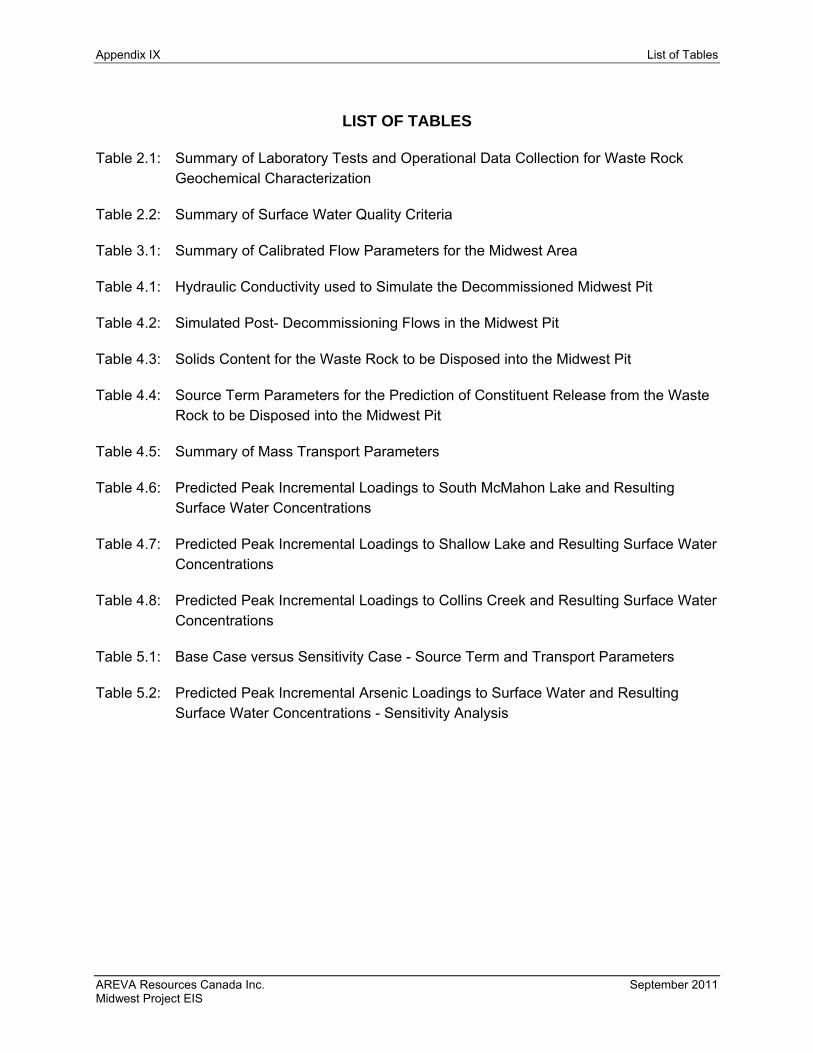
LIST OF TABLES

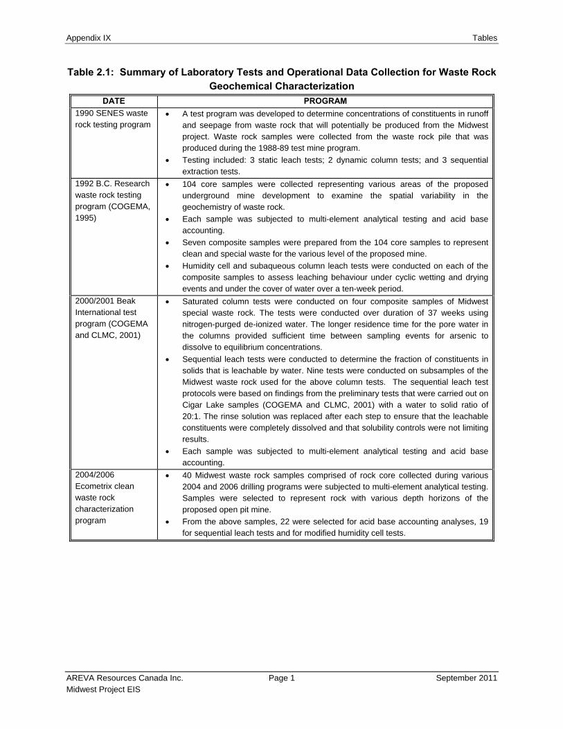
Table 2.1: Summary of Laboratory Tests and Operational Data Collection for Waste Rock Geochemical Characterization

Table 2.2: Summary of Surface Water Quality Criteria

Table 3.1: Summary of Calibrated Flow Parameters for the Midwest Area

Table 4.1: Hydraulic Conductivity used to Simulate the Decommissioned Midwest Pit

Table 4.2: Simulated Post- Decommissioning Flows in the Midwest Pit

Table 4.3: Solids Content for the Waste Rock to be Disposed into the Midwest Pit

Table 4.4: Source Term Parameters for the Prediction of Constituent Release from the Waste Rock to be Disposed into the Midwest Pit

Table 4.5: Summary of Mass Transport Parameters

Table 4.6: Predicted Peak Incremental Loadings to South McMahon Lake and Resulting Surface Water Concentrations

Table 4.7: Predicted Peak Incremental Loadings to Shallow Lake and Resulting Surface Water Concentrations

Table 4.8: Predicted Peak Incremental Loadings to Collins Creek and Resulting Surface Water Concentrations

Table 5.1: Base Case versus Sensitivity Case - Source Term and Transport Parameters

Table 5.2: Predicted Peak Incremental Arsenic Loadings to Surface Water and Resulting Surface Water Concentrations - Sensitivity Analysis

Appendix IX List of Figures

AREVA Resources Canada Inc. Page iv September 2011 Midwest Project EIS

LIST OF FIGURES

Figure 2.1: Limits of the Groundwater Flow Model for the Midwest Area

Figure 3.1: Summary of Hydraulic Conductivity Data for Sandstone

Figure 3.2: Cross Section Illustrating Groundwater Flow in the Midwest Area

Figure 3.3: Simulated Steady-State Hydraulic Heads in the Lower Sandstone Midwest Pre-Mining Conditions

Figure 4.1: Steady-State Pathline Analysis - Post-Decommissioning Flow Regime

Figure 4.2: Pathline Analysis Cross Section between the Midwest Pit and Collins Creek - Post-Decommissioning Flow Regime

Figure 4.3: Midwest Pond Water Quality - Potential Arsenic Concentrations

Figure 4.4: Predicted Arsenic Loadings from Placed Waste Rock to Surface Water Receptors

Figure 4.5: Predicted Arsenic Incremental Surface Water Concentrations

Figure 5.1: Sensitivity Analysis - Comparison between Realistic and Bounding Incremental Arsenic Loadings to Surface Water

Figure 5.2: Sensitivity Analysis - Predicted Arsenic Incremental Surface Water Concentrations

Appendix IX - Section 1 Introduction

AREVA Resources Canada Inc. Page 1 September 2011 Midwest Project EIS

1 INTRODUCTION

Post-decommissioning effects associated with the disposal of waste rock at the Midwest site derive from the release of soluble constituents from the waste rock to the groundwater system and subsequent transport to surface water receptors. The key components that control the release and transport of constituents include the chemical and physical properties of the waste rock and the groundwater flow regime in the Midwest area.

This appendix examines the above key components and provides estimates of post-decommissioning effects to surface water receptors resulting mainly from in-pit disposal of problematic waste rock. Summaries of the data, methods, and calculations used to assess the long-term environmental effects of waste rock management at the Midwest site are provided herein. The following outlines the contents of the various sections of this appendix:

Section 2.0 summarizes the methodology developed for the assessment of long-term environmental effects associated with waste rock management at the Midwest site.

Section 3.0 summarizes the characterization of the groundwater flow system in the Midwest area used in the assessment of potential long-term effects related to waste rock management. This is based on the work presented in Appendix IV (“Midwest Area Hydrogeology”), which includes a review of geological and hydrogeological data used to develop a three-dimensional flow model. This model forms the basis of the long-term predictions for contaminant mass loadings to receiving surface water bodies.

Section 4.0 summarizes the predicted long-term effects associated with waste rock management. Information provided in this section also summarizes Appendix VIII (“Waste Rock Characterization”), which includes a comprehensive description of the Midwest waste rock.

Section 5.0 discusses uncertainties in model predictions. The results of a sensitivity analysis are presented, which consider potential effects of uncertainties related to the groundwater flow system and the release of constituents from the waste rock.

Appendix IX - Section 2 Methodology for Long-Term Assessment


2 METHODOLOGY FOR LONG-TERM ASSESSMENT

Groundwater was identified as the principal pathway for potential interactions between constituents of the waste rock and the receiving environment. As a result, the assessment of long-term effects of waste rock disposal focused on the post-decommissioning groundwater flow regime in the Midwest area, the source terms (waste rock geochemical behaviour as a function of time) and the constituent release and transport mechanisms.

Field data acquisition, laboratory testing and modelling programs were developed to assess, as far as practical, the potential long-term effects of waste rock management activities.

2.1 Groundwater Flow Regime

A number of groundwater flow models were developed during the last 10 years for the McClean Lake Operation, including the Midwest area. A regional model was developed in 2003/2004 in order to reconcile previous flow models that, although having boundaries and/or surface areas in common, were not necessarily based on the same assumptions with respect to boundary conditions or distribution of hydraulic conductivity. The details of this work are presented in the Technical Information Document (TID) Hydrogeology and Groundwater Modelling of the Collins Creek Basin (COGEMA, 2004a).

A sub-model of the Midwest area was extracted from the regional model for the purpose of simulating groundwater flow during the operating and post-decommissioning periods. Details of the conceptual and numerical model are included in Appendix IV (“Midwest Area Hydrogeology”). The sub-model provides the basis for the solute transport analysis conducted for the Midwest area in its decommissioned configuration. The domain of the Midwest model is presented in Figure 2.1.

2.2 Source Term for Submerged Problematic Waste Rock

The following constituents were considered in the assessment of long-term effects: ammonia, chloride (Cl), sulphate (SO4), arsenic (As), cadmium (Cd), cobalt (Co), copper (Cu), lead (Pb), molybdenum (Mo), nickel (Ni), selenium (Se), vanadium (V), zinc (Zn), uranium (U), thorium-230 (230Th), radium-226 (226Ra), lead-210 (210Pb) and polonium-210 (210Po). Results presented in this appendix focus on key constituents for which predicted concentrations in receptors are not negligible.

The source term characterization for the waste rock was based on a series of sampling campaigns and laboratory tests that were carried out from 1981 to 2006, to evaluate the long-term behaviour of waste rock under various disposal/storage conditions. The initial characterization of waste rock provided estimates of materials inventory, special waste, clean



waste rock and overburden and respective uranium contents for the (then) proposed Midwest open pit (Canada Wide Mines Ltd., 1981). A comprehensive test program, which included humidity cell and saturated column testing followed this initial characterization. The saturated column test methodology and understanding of the rock/water interactions evolved over time. This led to the refinement of the test methodology for the column studies and sequential leach tests (COGEMA and CLMC, 2001). The comprehensive sampling database compiled during exploration of the Midwest area was further complemented with borehole sampling efforts conducted in 2004 and 2006. A number of sequential leach tests were subsequently carried out to better characterize the Midwest waste rock (see Appendix VIII). Overall, the Midwest waste rock characterization program involved chemical analysis of the rock, acid base accounting, humidity cell testing, customized leach tests to assess metal leaching, and flooded column tests to evaluate the “equilibrium” concentrations of key constituents of concern in pore water for an in-pit disposal scenario. Table 2.1 provides a summary of data collection and laboratory tests for waste rock characterization.

In a manner consistent with previous waste rock assessments (COGEMA and CLMC, 2001, COGEMA, 2004d) the arsenic source term for the current assessment was treated as a declining source function with decrease in constituent concentration with time. This simulated a waste rock pore water concentration that decreases with time as groundwater flows through the waste rock and decreases the constituent inventory remaining at the source. Two parameters are required to simulate such a source term: the initial pore water concentration and the source decay rate, which is derived from mass balance given the leachable mass in the waste rock and the flow through the waste rock. The mathematical expression that was used to simulate a declining source term corresponds to an exponential function as follows:

tCtC exp0 Equation 1

Where:

C0 = initial pore water concentration (M/L3);

= source decay constant (T-1); and

t = time (T).

The initial pore water concentration, C0, is known from the laboratory leaching tests. Therefore

the main unknown in the source term function is the parameter, . This parameter can be

calculated on the basis of mass balance. The total mass of solute released from the source is given by:

dttCQMMAXT

OUT 0 0 exp Equation 2



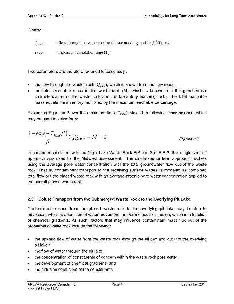
Where:

QOUT = flow through the waste rock to the surrounding aquifer (L3/T); and

TMAX = maximum simulation time (T).

Two parameters are therefore required to calculate :

the flow through the waster rock (QOUT), which is known from the flow model

the total leachable mass in the waste rock (M), which is known from the geochemical characterization of the waste rock and the laboratory leaching tests. The total leachable mass equals the inventory multiplied by the maximum leachable percentage.

Evaluating Equation 2 over the maximum time (TMAX), yields the following mass balance, which

may be used to solve for :

0

exp10

MQC

TOUT

MAX

Equation 3

In a manner consistent with the Cigar Lake Waste Rock EIS and Sue E EIS, the “single source” approach was used for the Midwest assessment. The single-source term approach involves using the average pore water concentration with the total groundwater flow out of the waste rock. That is, contaminant transport to the receiving surface waters is modeled as combined total flow out the placed waste rock with an average arsenic pore water concentration applied to the overall placed waste rock.

2.3 Solute Transport from the Submerged Waste Rock to the Overlying Pit Lake

Contaminant release from the placed waste rock to the overlying pit lake may be due to advection, which is a function of water movement, and/or molecular diffusion, which is a function of chemical gradients. As such, factors that may influence contaminant mass flux out of the problematic waste rock include the following:

the upward flow of water from the waste rock through the till cap and out into the overlying pit lake ;

the flow of water through the pit lake ;

the concentration of constituents of concern within the waste rock pore water;

the development of chemical gradients; and

the diffusion coefficient of the constituents.



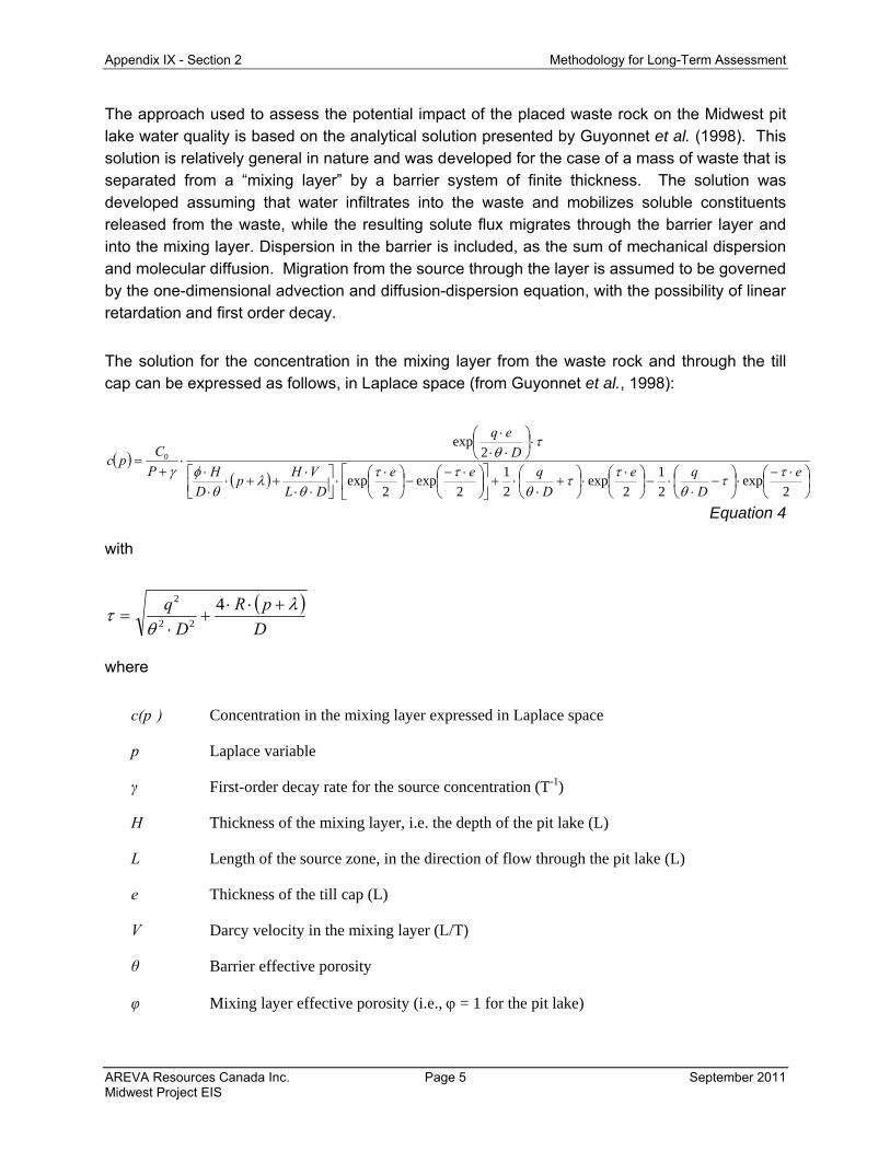
The approach used to assess the potential impact of the placed waste rock on the Midwest pit lake water quality is based on the analytical solution presented by Guyonnet et al. (1998). This solution is relatively general in nature and was developed for the case of a mass of waste that is separated from a “mixing layer” by a barrier system of finite thickness. The solution was developed assuming that water infiltrates into the waste and mobilizes soluble constituents released from the waste, while the resulting solute flux migrates through the barrier layer and into the mixing layer. Dispersion in the barrier is included, as the sum of mechanical dispersion and molecular diffusion. Migration from the source through the layer is assumed to be governed by the one-dimensional advection and diffusion-dispersion equation, with the possibility of linear retardation and first order decay.

The solution for the concentration in the mixing layer from the waste rock and through the till cap can be expressed as follows, in Laplace space (from Guyonnet et al., 1998):

2exp

2

1

2exp

2

1

2exp

2exp

2exp

0

e

D

qe

D

qee

DL

VHp

D

HD

eq

P

Cpc

Equation 4

with

D

pR

D

q

422

2

where

c(p ) Concentration in the mixing layer expressed in Laplace space

p Laplace variable

γ First-order decay rate for the source concentration (T-1)

H Thickness of the mixing layer, i.e. the depth of the pit lake (L)

L Length of the source zone, in the direction of flow through the pit lake (L)

e Thickness of the till cap (L)

V Darcy velocity in the mixing layer (L/T)

θ Barrier effective porosity

φ Mixing layer effective porosity (i.e., = 1 for the pit lake)



λ Constituent first-order decay rate (T-1)

q upward flow through the waste rock and out into the overlying till cap (Darcy flux) (L/T)

R Retardation factor

D Diffusion-dispersion coefficient through the till cap (L2/T)

The diffusion-dispersion coefficient (D) is defined as:

D = ( q / ) + DM

where:

longitudinal dispersivity (L)

DM molecular diffusion coefficient (L2/T)

Concentrations c(p) are transformed from the Laplace domain (inverse Laplace transformation) using the algorithm presented by de Hoog et al (1982).

Assuming a non depleting source term, the evaluation of Equation 4 at steady-state yields:

D

eq

Lq

HV

Cc

exp11

0 Equation 5

and the corresponding steady-state flux at the barrier/mixing layer interface is given by:

L

HVq

D

eqVHqLVH

qLCeF

exp

, 0 Equation 6

Equations 4 to 6 show that for very low values of q (i.e., negligible upward flow) the transfer of constituents from the waste rock to the overlying pit lake is essentially controlled by the magnitude of the diffusion coefficient through the till cap. In contrary, for large values of the upward flow the influence of diffusion is very limited and advection is the main mechanism controlling the transfer of constituents.



2.4 Solute Transport from the Submerged Waste Rock into the Surrounding Aquifer

The approach selected for simulating transport from the decommissioned Midwest area is based on the particle tracking method. This approach was developed in 2003 and was applied to both the Waste Rock Management area and the Tailings Management Area at the McClean Lake Operation (see Waste Rock Management TID and Tailings Management TID, COGEMA, 2004b and 2004c). This approach was also used as part of the Sue E EIS (COGEMA, 2004d). This method was used to calculate the mass of constituents of concern arriving at the surface water bodies over time, taking into account the groundwater flow velocity, dispersion, and attenuation along the flow pathway due to sorption behaviour and, when relevant, decay of the contaminant. The method consists of the following steps:

Step 1 - The particle analysis is performed using the calculation code MODPATH and the Visual MODFLOW environment. MODPATH allows forward and backward tracking particles to be released at specific locations within the flow domain. For the Midwest area, particles were located within the cells adjacent to the waste rock placed into the Midwest pit. These included cells within the formations (sandstone, regolith and basement) surrounding the edge of the Midwest pits and those corresponding to the pit lake. Finally, particles were also located within the cells simulating the surface waste rock stockpiles. The hydraulic head distribution calculated using MODFLOW is retrieved by MODPATH, which then calculates the flowpath followed by each particle assigned by the user. The output from MODPATH consists of an output file and of a visual reference for the flowpath for each particle, with time markers indicating the travel time between points based on the groundwater flow velocity. Travel times are calculated according to effective porosity values specified by the user. Each particle has a unique trajectory, which is a function of the overall groundwater velocity field and may vary from the horizontal to the vertical direction.

Step 2 – The output file generated by MODPATH (i.e., travel time as a function of travel distance, for each particle path) is used to calculate, for each path line, the total travel distance from the released location to the receptor and the average linear velocity along the path line.

Step 3 – A source term model is applied to calculate, as a function of time, a contaminant concentration at the location of the released particles.

Step 4 – The advection-dispersion equation is solved analytically for each path line, using the concentration calculated in Step 3 as boundary condition. The concentration at the end of the path line (i.e., at the receptor) is calculated as a function of time.

Finally, all the particle paths are integrated to calculate the mass flux arriving at the receptor, given the flow associated with the path lines. The corresponding flow is calculated from the flow model. This approach presents several advantages. It is fast, easy to implement, and does not include numerical uncertainties since the advection-dispersion along each path line is solved analytically. The approach also includes some conservatism since it does not account for lateral dispersion; the procedure includes only a longitudinal dispersion along each path line.



The analytical solution selected to simulate contaminant transport along each path line is very general in nature. It was developed (van Genuchten, 1985) for a semi-infinite one-dimensional configuration to simulate transport of four solutes involved in sequential first-order decay reactions. Various boundary conditions can be considered, including concentration-type or flux-type conditions declining or pulse-type input functions.

The solution considers the following set of coupled differential equations:

Species 1

11

21

21 CR

x

Cu

x

CD

t

CR

Equation 7

Species 2, 3, and 4

1112

2

iiiiii

iiX

ii CRCR

x

Cu

x

CD

t

CR Equation 8

i = 2, 3, 4

with

e

Dn

Vu and e

DD n

KR 1

where

VD =Darcy velocity (L/T)

u =pore water velocity (L/T)

R =retardation factor

D =bulk dry density (M/L3)

KD =distribution coefficient (L3/M)

ne =effective porosity (-)

Dx =dispersion coefficient in the direction of flow (L2/T)

t = time (T)

x =position in the direction of flow (L)



C =solute concentration (M/L3)

=first-order decay rate (T-1)

The reader is referred to van Genuchten (1985) for the expression of the analytical solution. Transport of arsenic and other stable constituents was simulated using equation for species 1

(Equation 7) only, without considering the decay constant (=0). The set of coupled governing

equations was used to simulate transport of thorium-230, radium-226 and lead-210.

2.5 Case of the Clean Waste Rock Piles

The waste rock segregation procedure proposed for the Midwest project involves the coupled use of radiometric probing for uranium detection and portable XRF analysis for arsenic detection. This proposed procedure is intended to distinguish between potentially problematic materials that may require in pit disposal and underwater storage from those that may be safely stored above grade, on land. As arsenic is identified as the key constituent of concern a

relatively low cut-off level for arsenic (i.e., 75 g/g) is proposed to segregate problematic waste

rock from clean waste rock.

The waste rock characterization programs (see Appendix VIII) indicate that the material to be stored on land will exhibit virtually no risk of acid generation and is expected to produce low concentrations of constituents of concern. Monitoring of clean waste rock stockpile leachate will be conducted during operations to confirm the findings of laboratory testing conducted on similar material, which formed the basis for the proposed management strategy for this material.

2.6 Significance of Predicted Surface Water Concentrations

The predicted long-term concentrations of constituents of concern in surface water receptors, which derive from waste rock management, were compared to baseline concentrations, currently applicable water quality objectives and aquatic toxicity benchmarks (Table 2.2).

Appendix IX - Section 3 Conceptual and Numerical Hydrogeological Model


3 CONCEPTUAL AND NUMERICAL HYDROGEOLOGICAL MODEL

3.1 Conceptual Hydrogeology

The geology of the Midwest area, relevant to the development of a conceptual and numerical groundwater flow model, consists of 3 units: 5 to 20 m of overburden (glacial till deposits) underlain by approximately 200 m of sandstone, underlain by basement rock.

The groundwater regime in the area consists of two flow systems. A shallow flow system occurs in the glacial deposits, which act as a shallow unconfined aquifer, and is controlled by recharge from precipitation and interactions with numerous lakes. The deep flow system comprises mainly groundwater flow in the underlying sandstone unit. The information provided by the geological and hydrogeological database is summarized by the following discussion.

Hydraulic Conductivity

Laboratory determination of saturated hydraulic conductivity indicates that the hydraulic conductivity of the sandstone matrix is very low, around 10-9 m/s. However, the sandstone unit is fractured on both the local and regional scales and fracture-enhanced permeability is observed. In particular, vertical structures with an approximately northeast-southwest orientation are considered to be preferential indicators to identify higher permeability zones. Conglomerate-enhanced permeability is also observed, mainly in the basal member of the sandstone unit. Pumping test results suggest that a value of 3 x 10-6 m/s is representative of the overall hydraulic conductivity of the sandstone unit, which constitutes the main aquifer over the project area. The average hydraulic conductivity of the basement rock is around 3x10-8 m/s. Figure 3.1 illustrates the statistical distribution of hydraulic conductivity in the sandstone.

Role of Lakes

The numerous surface water bodies of the project area appear to play different roles with respect to interaction with the groundwater flow system.

The McClean Lake/Collins Creek area appears to be a regional discharge zone, including for groundwater originating from the Midwest area. Piezometric data show that the deep groundwater flow converges to this area. Groundwater chemistry and environmental isotope data (low tritium concentration) may also indicate that relatively deep groundwater is discharging in this area.

Numerous lakes act as local discharge zones, mainly to the overburden aquifer, and to some extent to the sandstone. The Mink arm of South McMahon lake appears to an example of local discharge zones. Lakes located in upland areas appear to be part of recharge zones.



Figure 3.2 provides a schematic cross-section of the conceptual model of groundwater flow in the Midwest area. Groundwater flow is generally horizontal and in the southeast direction in the lower sandstone.

Midwest Groundwater Modelling

Figure 2.1 shows the limits of both the regional model and the Midwest local model. The three-dimensional flow model developed for the Midwest area is a ‘living tool’ subject to improvements of both the conceptual and numerical components, as information continues to be collected in coming years. In its current status, the model covers an area that extends from Henday Lake to Collins Creek. It corresponds to a domain of approximately 236 km2. The grid is centered on the location of the proposed open-pit, with grid rows aligned with the dominant direction of groundwater flow (i.e. north-west to south-east). The model has 14 layers, 183 columns and 207 rows and a grid size ranging from 300 m to less than 10 m in some areas around the proposed Midwest pit.

Both uninfluenced steady-state ‘pre-mining’ and influenced transient conditions (i.e., pumping test, dewatering of Mink Arm, test mine) were used to calibrate the model. The calibration process in groundwater modelling is non-unique, which means that there may be several sets of model parameters that provide an acceptable fit between observed and calculated data. However, usually, when several sets of observations are used to calibrate the model, there is only a narrow range of parameters that may fit all observations and interpretations within a reasonable range of measurements and associated estimates. For the Midwest area, several hydraulic conductivity distributions were found to provide reasonable calibration results. Three distributions were selected based on the following criteria:

they provide an acceptable fit between observed and simulated data both under steady-state and transient conditions,

they are relatively simple,

they are consistent with the packer test and pumping test results; and,

they tend to provide conservative estimates in the sense that the inflows predicted with these distributions tend to be higher than the observed inflows. This conservative approach is considered to be appropriate for the purpose of estimating post-decommissioning flows.

Table 3.1 includes a summary of calibrated flow parameters for the Midwest area. Two zones were calibrated in the overburden layer with hydraulic conductivity ranging from 4 x 10-7 m/s to 1x10-5 m/s. In the upper part of the sandstone unit the calibrated values range from 4x10-7 m/s to 3 x 10-6 m/s. In the lower part of the sandstone the calibrated values range from 4 x 10-7 m/s to 4 x 10-6 m/s. Values ranging from to 8 x 10-6 m/s to 1 x 10-5 m/s are calibrated for the basal conglomerate. A horizontal hydraulic conductivity (Kh) of 2 x10-7 m/s and a vertical hydraulic conductivity (Kv) of 1 x 10-7 m/s were calibrated for the altered formation (i.e., the regolith) separating sandstone from unaltered basement rock formation. A value of 2 x 10-8 m/s was



calibrated for the basement rock (2 ≤ Kh/Kv ≤10). Finally, a value of 5 x 10-7 m/s was considered to be representative of the alteration halo associated with the Midwest deposit.

Overall, the model reproduces the pre-mining flow conditions relatively well in the areas where pre-mining data are available with calibration results that meet calibration targets. The overall calibration error (i.e., Normalized Root Mean Square Error) for the pre-mining steady state groundwater flow model is lower than 10% and the observed drawdown and inflows during pumping tests and the test mine are reasonably simulated.

Contours representing the calculated baseline hydraulic head distribution for the lower sandstone are shown in Figure 3.3. The sandstone formation is considered for this figure as most of the groundwater flow occurs in this aquifer. The figure shows that groundwater flow in the sandstone is directed to the southeast, from Henday Lake to McClean Lake/Collins Creek.

Appendix IX - Section 4 Long-Term Effects Related to Waste Rock Management


4 LONG-TERM EFFECTS RELATED TO WASTE ROCK MANAGEMENT

4.1 Waste Rock Disposal Option

The proposed long term waste rock disposal option in the Midwest area involves the placement of all problematic waste rock in the mined out Midwest Pit. A two-meter compacted till cap will be placed on top of the waste rock upon decommissioning. The primary objective of the till cap is to limit the upward flow from the waste rock into the overlying pit lake. Following decommissioning, the Midwest pit will be allowed to be re-flooded until water levels in the pit reach a steady state condition.

As an alternative to this decommissioning plan, the Midwest pit could be entirely backfilled. Under this scenario, the problematic waste rock would be placed at the bottom of the pit and a fraction of the clean waste rock would be used to entirely backfill the pit. The main advantage of this alternative decommissioning plan would be to eliminate the potential for a long-term water quality issue of the Midwest pit lake. In addition, this option would reduce the volume of material to be managed in clean waste rock piles from approximately 46 Mm3 to 12 Mm3 (lcm). An obvious disadvantage of the fully backfilled pit option is its cost. Therefore, the fully backfilled pit is analyzed as a backup decommissioning plan for the Midwest pit, should the pit lake water quality evolve unacceptably and should the water treatment plant be unable to treat the pit lake water.

Based on waste rock characterization and block modeling results (see Appendix VIII), the volume of problematic waste rock is estimated to range between 930,000 m3 (bcm) and 1,400,000 m3 (bcm). Based on a swelling factor of 1.35, the volume of waste rock to be disposed in the Midwest pit would range between 1,255,500 loose cubic metres (lcm) and 1,890,000 lcm, which would fill the Midwest pit to a maximum elevation of 328 mASL. It is expected that, by application of field screening for metals content, the actual volume would fall toward the lower end of the range presented above. However, as a conservative approach, the volume of special waste rock requiring in pit disposal has been taken as 2.5 Mm3 (bcm) for the purpose of this assessment. This increased volume was used both to simulate the post-decommissioning flow regime and to simulate the source term for the placed waste rock. A volume of 2.5 Mm3 (bcm) translates to a loose volume of approximately 3.4 Mm3, which would fill the Midwest pit to an elevation of approximately 335 mASL.

A non conservative approach would be to adopt a grade of 425 µg/g of uranium to define ore as opposed to 850 µg/g of uranium used in the calculations above. This would result in lower quantities of special waste to be disposed of in the Midwest pit and higher quantities of tailings to be managed in the JEB TMF. At the JEB TMF, the additional quantities of tailings that would be generated if a lower cut-off level was used would marginally affect the capacity of the TMF. From a contaminant content perspective, the robustness of the TMF would not be affected because the tailings preparation circuits would not be modified. In addition, as arsenic



concentrations tend to increase with uranium concentrations (Appendix VIII, Table 3.1), using a lower cut-off level for uranium would result in a lower arsenic content of the additional ore to be processed.

4.2 Post-Decommissioning Flow Regime

4.2.1 Assumptions

The post-decommissioning flow regime was modelled based on the groundwater flow model presented in Section 3 and assumptions regarding the hydraulic conductivity of the waste rock to be disposed into the pit and the hydraulic conductivity of the till cap to be constructed over the waste rock. Table 4.1 presents hydraulic conductivity values that were applied to simulate placed waste rock. The hydraulic conductivity of all waste rock to be placed in the Midwest pit (i.e., special waste up to elevation 335 mASL and clean waste rock from 335 mASL to ground surface) was conservatively assumed to be 10-4 m/s.

The clean waste rock piles were included in the modelling of post-decommissioning groundwater flow. The infiltration rate through the waste rock piles was considered to be similar to the rate of groundwater recharge for the drumlin areas, with values ranging from 55 mm/year to 80 mm/year (Appendix IV, Section 3.4.1.2).

Post-decommissioning flow simulations were conducted for the three distributions/cases of hydraulic conductivity selected during the calibration phase (see section 3.2 and Table 3.1).

4.2.2 Flow Balance

Groundwater flow simulations were performed under steady state conditions, as would exist following decommissioning, in order to calculate the groundwater flow rates through the waste rock and the water column of the flooded pits for different scenarios. These simulations constitute the basis for the long-term contaminant transport assessment. The flow rates were calculated using the ZONE BUDGET option of Visual MODFLOW. The calculated steady-state flow rates are tabulated in Table 4.2.

For the three cases, the final elevation of the till cap in the Midwest Pit is 337 mASL. The calculated flow through the waste rock and out into the surrounding aquifer ranges from 17 m3/day for Case 1 to 41 m3/day for Case 3. Overall, the material to be placed in the Midwest pit has a hydraulic conductivity relatively similar, or slightly higher, to the original rock mass. By comparison, the overlying pit lake has an ‘infinite’ hydraulic conductivity, and consequently, the main component of the groundwater flow into the pits is directed towards the pit lake. The contrast in hydraulic conductivity between a highly permeable pit lake and the less permeable



underlying waste rock provides a favourable flow configuration, which tends to limit the flow through the placed waste rock.

The upward flow from the waste rock through the till cap and into the Midwest pit lake was calculated to be negligible. The downward flow from the pit lake through the till cap and into the waste rock is significant, ranging from approximately 20 m3/day (Case 1) to 50 m3/day (Case 3). With this downward flow, it can readily be shown that the upward transport of constituents will be negligible as the downward flow opposes the upward migration. The total flow through the reflooded Midwest pit water column is calculated to range from 150 m3/day to 200 m3/day.

The effect of the pit lake on the groundwater flow regime was simulated as part of the post-decommissioning flow simulations used above. Simulations suggest that the Midwest pit lake will not be connected to South McMahon and will act as an isolated surface water body connected to the groundwater flow system. Once the long term pit lake equilibrium is established, both groundwater and precipitation/surface runoff entering the pit lake will leave the pit lake area by groundwater outflow essentially through the overburden and upper sandstone layers and by evaporative losses.

As an example, Figure 4.1 shows the calculated steady state distribution of hydraulic head in the upper sandstone for Case 1 (see definition of Case 1 in Appendix IV, Section 3.4 and predicted post-decommissioning impacts for Case 1 in Appendix IX, Section 4.5). The pit lake acts as a zone of large hydraulic conductivity resulting in a relatively flat piezometry with a small hydraulic gradient through the pit lake area, as opposed to the surrounding formation. Similar conditions are predicted to occur for Case 2 and 3.

The impact of the waste rock piles on the post-decommissioning groundwater flow conditions appears to be very limited. The waste rock piles act essentially as a non saturated zone and the water table is established in the overburden layer at the base of the piles (Figure 4.2).

In the case of the fully backfilled pit option, for each of the three cases outlined (Appendix IV, Section 3), two values were considered for the net infiltration through the top layer of the backfilled pit for sensitivity analysis purposes. The first was 55 mm/year which is a value similar to the average groundwater recharge rate. The second, 150 mm/year, was a value expected for a non compacted waste rock pile.

Figure 4.3 illustrates the steady-state distribution of hydraulic heads in the upper sandstone of the Midwest area as simulated by the model for Case 1 and the fully backfilled pit option. This figure shows that the groundwater flow conditions for the fully backfilled pit option appear to be very similar to the groundwater flow conditions for the partially backfilled and flooded pit option. This is consistent with the value of the hydraulic conductivity used to simulate the waste rock to be placed in the upper part of the Midwest pit. The selected value (10-4 m/s) is approximately



two orders of magnitude greater than the hydraulic conductivity of the surrounding rock mass and consequently the backfilled pit tends to act as a drain in a manner relatively similar to the pit lake for the partially backfilled and flooded pit option.

The flow through the clean waste rock and out into the surrounding aquifer is calculated to range from approximately 80 m3/day (Case 3, infiltration of 55 mm/year) to 208 m3/day (Case 1, infiltration of 150 mm/year). A fraction of this flow, especially for Case 1 and Case 2, is expected to report to the surface water receptors located between the Midwest area and Collins Creek.

4.2.3 Particle Path Analysis

Figure 4.4 illustrates the steady-state distribution of hydraulic heads and the results of particle path analysis in the lower sandstone unit of the Midwest area for the three cases. The lower sandstone formation is considered because it constitutes the principal hydrostratigraphic unit, in which most of the groundwater flow takes place.

Figure 4.4 shows that for Case 3 particles originating from the placed waste rock in the Midwest pit discharge only to Collins Creek over a distance of about 2 to 2.5 km. In addition, for Cases 1 and 2, some particles also discharge to South McMahon Lake and to Shallow Lake. Figure 4.5 presents a cross-section of the area between the Midwest Pit and Collins Creek with particle tracking results that illustrate the groundwater flow paths for Case 3. The path lines in Figure 4.5 shows that the basal conglomerate acts as a drain and that deep groundwater within the waste rock flows to Collins Creek.



4.3 Release from Placed Waste Rock to the Surrounding Aquifer

Solid Content

Table 4.3 provides a comparison of solids content of the Midwest special waste rock that was considered previously for the Sue E EIS (COGEMA 2004d) and that was considered for this assessment. The current estimate is based on the development of an open pit mine, which generates more waste at lower grades in relation to an underground mine development, as was previously considered.

Table 4.3 presents the solids concentrations used for this assessment for each constituent of concern. For arsenic and uranium the values correspond to the average of the block model estimates (Appendix VIII). For the other constituents the selected values have been estimated by averaging the solids contents of all samples used to characterize the problematic waste rock (i.e., 1980, 1995 and 2001 programs, Table 4.1, Appendix VIII).

Leachable Mass and Pore Water Concentrations

Table 4.4 summarizes the source term parameters used to characterize the Midwest problematic waste rock. Based on a volume of 2.5 Mm3 (bcm) and a density of 2.4 t/m3, the total mass of problematic waste rock considered for this assessment is 6 million tonnes.

Arsenic

The average solid arsenic concentration is calculated to be 1,100 g/g. Two key parameters are

required to simulate the leaching of arsenic from the placed waste rock: the initial arsenic pore water concentration and, the leachable mass. Interpretation of column test results for arsenic indicates that there is a relationship between arsenic concentrations in the waste rock pore water and the total arsenic content of the waste rock (i.e., solid arsenic content). This relationship is discussed in Appendix VIII and has been used to determine initial arsenic pore water concentrations representative of waste rock to be disposed of within the Midwest Pit. Using the relationship between solids arsenic content and pore water concentration, the pore water concentration for the Midwest problematic waste rock is estimated to be 86 mg/L. The change in waste rock arsenic pore water concentrations with time is constrained by the total leachable mass of constituents (i.e., mass available for release) in the waste rock. Interpretation of sequential leach tests for arsenic indicates that there is a relationship between water leachable arsenic concentrations and the total arsenic content of the waste rock (i.e., solid arsenic content). This relationship is discussed in Appendix VIII and has been used to determine the arsenic leachable mass representative of waste rock to be disposed into the Midwest. The water leachable arsenic mass is estimated to be proximately 768 tonnes.



Other Constituents

For molybdenum, a leachable fraction of 42% was selected, which corresponds to the average of the 2001 sequential extraction tests. For the remaining constituents, for simplicity and conservatism, the leachable fractions selected correspond to values previously presented in the Sue E EIS for the Midwest special waste rock. These values are on the conservative side. For instance, the water leachable fraction for cobalt, copper, nickel, lead and zinc ranged from 0.01% to 1%. A value of 1.5% was selected for the assessment.

A constant source concentration, until release of the maximum leachable mass (i.e., pulse-type function) was assumed. The two parameters required for this approach are, for each constituent, the value of the constant source concentration and the duration of the pulse. The constant source concentration was determined from the laboratory tests. The duration of the pulse was determined according to the flow through the waste rock.

Clean waste rock

The results of the clean waste rock characterization (Appendix III) show that sulphide-sulphur content of the clean rock is very low and there is virtually no risk of acid generation from this material, even if the rock is stored on land. With respect to metal leaching, arsenic (i.e., the key constituent of concern) was found to be below detection limits in leachate associated with leach tests under oxygenated conditions. The application of robust segregation criteria will ensure that this rock has low levels of constituents of concern. Therefore, mass transport from the clean waste rock piles and clean waste rock portion of the entirely backfilled pit option was not included in the contaminant transport model.

As indicated in Appendix VIII, it is proposed to construct the surface waste rock stockpiles with perimeter ditches to collect runoff and leachate seepage from the piles. Monitoring of the quality of this water during operations will be conducted to confirm the acceptability of surface disposal as a long term clean waste rock management plan. It is also planned to install groundwater monitoring wells around the waste rock piles to monitor trends in groundwater quality.

4.4 Mass Transport Parameters

Using the output from MODPATH, the advection-dispersion equation was solved analytically for each particle path (see section 2.3). Approximately 100 particles were located in the Midwest Pit to simulate mass transport from the placed waste rock, for the three cases of hydraulic conductivity distributions. Therefore, each simulation included approximately 100 particle paths and, subsequently, the advection-dispersion equation was solved approximately 100 times for each simulation. Input parameters for solute transport calculations are summarized in Table 4.5. With the exception of sulphate and chloride, sorption behavior along the groundwater flow path



was accounted for all constituents using the concept of a linear, instantaneous and fully reversible sorption process.

Travel Distance

The travel distance (x) was calculated directly from the particle paths analysis. Each particle path has its own flow path length. The calculated distances from the Midwest Pit to Collins Creek range from approximately 6,500 to 8,100 m. The calculated travel distance from the Midwest C pit to South McMahon Lake ranges from approximately 1,450 m to 1,600 m and the calculated travel distance from the Midwest Pit to Shallow Lake is on the order of 2,000 m.

Pore Water Velocity

The pore water velocity (v) was calculated directly from the particle paths using an effective porosity of 11%. This value is based on laboratory testing that was conducted on sandstone samples from the JEB site (COGEMA, 1997, Table 12.2-5-1). Each particle path is associated with a distinct average groundwater velocity. The calculated velocity ranges from 0.05 m/year to 17 m/year.

Dispersivity

Dispersivity is generally recognized to increase with flowpath distance. Literature review indicates that in general longitudinal dispersivity is observed to be approximately 10% of the flow path distance (based on tracer tests and observation of contaminant events). As such, the longitudinal dispersivity was systematically taken to be 10% of the travel distance of each particle. As a result, dispersivity values that were used in mass transport simulation range from 145 m to 810 m.

Distribution Coefficient

Distribution coefficient (Kd) values determined for sandstone and sand at Cigar Lake, Key Lake and Midwest sites ranged from 1 L/kg to 100 L/kg for arsenic (COGEMA and CLMC, 2001, Table 3.0, Appendix II). Arsenic Kd was conservatively assumed to be 1 L/kg. Given the effective porosity of 11% and a bulk dry density of 2.36 kg/L (typical sandstone value in this area), a Kd of 1 L/kg translated to a retardation factor of approximately 22.5. That is to say that arsenic would move at a rate about 22.5 times slower than groundwater.

Radium sorption tests were conducted on sandstone samples (COGEMA, 1997). Radium-226 distribution coefficient values were found to range from 3.8 L/kg to 128 L/kg for sandstone units within the Athabasca basin. Results specific to sandstone samples collected from the JEB site indicated a distribution coefficient of 50 L/kg for sorption of radium-226 onto altered sandstone. Based on these results the lowest (conservative) value of 3.8 L/kg was selected to simulate transport of radium-226.



For simplification purposes, the remaining constituents of concern were assigned a value of one, as for arsenic. This translates to a relatively conservative assumption.

4.5 Surface Water Quality Predictions

The loadings of constituents of concern to surface water receptors, and the resulting surface water concentrations, are presented in this section. The assessment included all the surface water bodies that may be affected over the long term (i.e., 15,000 years) by shallow and deep groundwater flow from the Midwest area. These include Collins Creek, South McMahon Lake, Shallow Lake and Midwest Pit Lake.

4.5.1 Midwest Pit Lake

The Midwest pit lake water quality was estimated using the approach described in section 2.3. Attenuation in the till cap was ignored, adsorption onto pit lake sediments was not included, and the loading of constituents into the pit lake was considered constant, disregarding mass loss into the surrounding aquifer. The pit lake system was considered to be at equilibrium (i.e., steady-state flow conditions, no pit lake evaporation and no chemical processes). Concentrations of constituents in the pit lake were calculated from the net flux of solutes from pore water in the waste rock resulting from upward advection/dispersion through the 2 m till caps that overlie the waste rock.

The following input parameters were also used:

The effective porosity of the till cap was taken as 10%

Values ranging from 5 x10-11 m2/s to 4.4 10-10 m2/s were considered for the molecular diffusion coefficient used to simulate the diffusive movement of arsenic through the till cap. A mean value of 1 x10-10 m2/s was assumed. This value is considered to be relatively conservative. For instance a molecular diffusion coefficient of 3.0x10-11 m2/s was estimated for arsenic from radial diffusion tests conducted on sandstone core from the JEB site (COGEMA 1997).

Longitudinal dispersivity was taken to be 20 cm; that is 10% of the thickness of the cap on top of the waste rock

The long-term arsenic concentration within the submerged problematic waste rock was taken to be 86 mg/L in a manner consistent with the assumption made to simulate the release of arsenic from placed waste rock to the surrounding aquifer (section 4.6).

Figure 4.6 presents predicted long-term concentrations in the Midwest pit lake as function of both the upward flow from the waste rock through the till cap and the value of the diffusion coefficient. The upward flow from the waste rock through the till cap and into the Midwest pit lake was calculated to be negligible and a maximum value of 1 m3/day was considered for the



purpose of this assessment. Assuming the pit lake acts as a full mixing layer, the predicted pit

water quality for arsenic would range from a few g/L to 0.6 mg/L, approximately.

However, a review of water quality of abandoned pit lakes suggests that the full mixing assumption is not appropriate for pit lakes with a relatively large relative depth. Relative depth can be defined as a percentage as follows (Castro and Moore, 2000):

A

ZD M

R 50 Equation 9

Where:

Zm = the maximum depth of the lake; and

A = the surface area of the lake.

Most natural lakes have DR values of less than 2%, and very few yield values in excess of 5%. By contrast, mine pit lakes may have DR values in the range 10% to 40%. The high DR values promote the development of multi-layers systems in which the deepest layer is never involved in seasonal overturn. This deepest layer is usually cold, dense, containing the most mineralized water in the lake and remaining stagnant.

Once flooded, the final depth of water in the Midwest pit will be approximated 143 m, with a surface area of 415,000 m2. As a result, the corresponding relative depth of the pit will be approximately 20%. This relative depth is sufficient to anticipate the formation of a permanent chemocline within the water column of the pit. In the medium and long-term, chemocline formation will result in a meromictic state, where water below the chemocline does not mix with water above the chemocline. This will serve to permanently isolate potentially contaminated groundwater in the lower reaches of the pit, minimizing the potential interaction with surface water receptors.

4.5.2 Surface Water Receptors

For illustration purposes, mass flux and incremental solute concentrations of arsenic are plotted with respect to time for the three hydraulic distribution cases in Figures 4.7 and 4.8. Peak arsenic concentrations are simulated to occur at approximately 7,000 years for Collins Creek and after 10,000 years for the other two key receptors (South McMahon and Shallow Lake). Figures 4.7 and 4.8 also show that the first loadings are predicted at approximately 2,000 years.



At 15,000 years, the cumulative mass of arsenic released to surface water corresponds to approximately 50% of the total mass released from the waste rock.

For the fully backfilled pit option flow through the special waste (i.e., located between the bottom of the pit and elevation 335 mASL) and out into the surrounding aquifer was calculated to range from approximately 13 m3/day (Case 1, infiltration of 55 mm/year) to 42 m3/ day (Case 3, infiltration of 150 mm/day). These values are similar to the ones calculated for the partially backfilled and flooded pit option. This suggests that the two decommissioning options are not expected to differ significantly in terms of impact of special waste to surface water receptors (i.e., similar incremental loadings and resulting long-term surface water concentrations.

South McMahon Lake

Under cases 1 and 2 of hydraulic conductivity distribution, South McMahon Lake may be affected by groundwater flow through the waste rock placed in the Midwest pit because some groundwater flow originating from the Midwest area discharges into this lake. The average annual flow out of South McMahon Lake (i.e., about 5,530 m3/day) was used to calculate the incremental surface water concentration. For arsenic, the maximum calculated flux is predicted to range from 1.7 kg/year for Case 1 to 3.6 kg/year for Case 2. Table 4.6 presents predicted peak total loadings to South McMahon Lake and the resulting peak incremental solute concentrations. The arsenic peak concentration in South McMahon is predicted to range from

0.8 g/L for Case 1 to 1.8 g/L for Case 2. These values range between the mean baseline

concentrations and the CCME water quality objectives. For the other constituents of concern, the predicted concentrations are lower than the mean baseline concentrations. Under Case 3 of hydraulic conductivity distribution, South McMahon Lake is not affected by groundwater flow through the submerged waste rock.

Shallow Lake

Under case 1 and 2 of hydraulic conductivity distribution, Shallow Lake may be affected by groundwater flow through the waste rock placed in the Midwest pit. The average annual flow out of Shallow Lake (i.e., about 2,508 m3/day) was used to calculate the incremental surface water concentration. For arsenic, the maximum calculated flux is predicted to range from 1.4 x 10-6 kg/year for Case 1 to 3 kg/year for Case 2. Table 4.7 presents predicted peak total loadings to Shallow Lake and the resulting peak incremental solute concentrations. The arsenic peak

concentration in Shallow Lake is predicted to range from negligible values for case 1 to 3.2 g/L

for case 2. This value ranges between the mean baseline concentrations and the CCME water quality objective. For the other constituents of concern, the predicted concentrations are lower than the mean baseline concentrations. Under Case 3 of hydraulic conductivity distribution, Shallow Lake is not be affected by groundwater flow through the submerged waste rock.



Collins Creek

Water quality in Collins Creek may be affected by constituent loadings transported by groundwater from the Midwest pit. The average annual flow in Collins Creek over the area where the plume could potentially discharge (i.e., about 118,714 m3/day) was used to calculate the incremental surface water concentration. Table 4.8 presents predicted peak total loadings to Collins Creek and the corresponding peak incremental solute concentrations. For arsenic, the maximum calculated flux is predicted to range from 1.8 kg/year for Case 1 to 79 kg/year for Case 3. The resulting maximum peak arsenic concentration is predicted to be on the order of

1.8 g/L for Case 3. This value ranges between the mean baseline concentrations and the

CCME water quality objective. For the other constituents of concern, the predicted concentrations are lower than the mean baseline concentrations.

Appendix IX - Section 5 Sensitivity Analysis


5 SENSITIVITY ANALYSIS

5.1 Methods

For the assessment of the long-term effects, uncertainties were handled through a deterministic approach. Extreme values were first selected for the key parameters that have a significant impact on the calculated loadings to receptors and resulting surface water concentrations. Then, simulations were carried out with these extreme values to assess the combined effects of varying the key parameters simultaneously in the direction that increases the calculated concentrations. This included considering daily low flow conditions in surface water to calculate surface water concentrations resulting from the maximum loadings predicted over the next 15,000 years.

Sensitivity analyses were performed for a number of scenarios to assess source term (waste rock pore water concentrations, leachable mass, flow through waste rock) and transport pathway uncertainties (i.e., groundwater velocity, dispersivity, sorption behaviour). Key parameters of the sensitivity analysis are reviewed in the following section. Table 5.1 summarizes the key parameters for the sensitivity analysis.

Arsenic has been shown to be more soluble relative to other constituents of concern and therefore the sensitivity analysis focussed on arsenic. The ratios of other constituents of concern concentrations to their respective water quality objectives are all lower than that for arsenic and the Kd values are the same or higher. This means that the margin of safety to the receiving environment for other constituents of concern will be greater than that of arsenic.

5.1.1 Source Term Parameters

Solid Concentration

The volume of Midwest problematic waste rock was estimated to range between 930,000 m3 (bcm) and 1,400,000 m3 (bcm) and the corresponding average arsenic content was determined

to range between 980 g/g and 1,500 g/g (Appendix VIII). For the base case, a conservative

volume of 2,500,000 m3 and an average arsenic solid content of 1,100 g/g were considered.

This average concentration was increased to 1,500 g/g for the sensitivity analysis.

Leachable fraction

For the sensitivity analysis, the extreme case for leachable arsenic was estimated using the power function for total leachable arsenic (i.e., leachable mass calculated from sequential extraction tests with weak phosphoric acid steps) and the relationship (see Appendix VIII):

Soluble Arsenic = 0.0467 (Total Solid Arsenic Content )1.2335



This relationship provides a reasonable upper bound for the water-leachable fraction of arsenic.

Initial Pore Water Concentration

The extreme case for the initial arsenic pore water concentration was estimated as a function of the arsenic content in the solid using the following power function (see Appendix VIII):

Arsenic Pore Water Concentration (mg/L) = 0.123 (Total Solid Arsenic Content)0.935

Based on this relationship, the initial arsenic pore water concentration in the flooded Midwest problematic waste rock would be on the order of 115 mg/L. As described in Section 12 of the Main Document, one objective of the proposed waste rock follow-up program is to assess the realism and the level of conservatism of this relatively high concentration.

Flow through Waste Rock

For the base case, the estimated flows through the waste rock were calculated for three hydrogeological scenarios, providing a first sensitivity analysis. A high hydraulic conductivity (i.e., 10-4 m/s) was also conservatively used to simulate the placed waste rock. In addition, for the sensitivity case, the calculated flows through the waste rock were systematically increased by 15% to account for model uncertainty in flow predictions. A similar approach was used as part of the sensitivity analysis for the Cigar Lake Waste Rock EIS (COGEMA and Cameco, 2002).

5.1.2 Transport Parameters

The approach used as part of the Cigar Lake Waste Rock EIS and the Sue E EIS was re-used; that is:

The velocity along each path line was increased by a factor 4. The Cigar Lake Waste Rock EIS showed that increasing the velocity by a factor of 4 was a reasonable assumption to account for uncertainties in hydraulic conductivity and hydraulic gradient between the Sue area and Collins Creek.

The dispersivity along each path line was decreased by a factor of 2, resulting for each path line a dispersivity equal to 5% of the traveled distance. A decrease in dispersivity results in an increase in peak concentration.

A Kd of 1 L/kg was assumed for arsenic for both the realistic case and the sensitivity analysis. The value of Kd = 1 L/kg corresponds to the lowest value measured for the Athabasca basin. It is also consistent with the lowest default value recommended for arsenic for environmental assessments (Thibault et al., 1990).



5.1.3 Flow in Surface Water

For the sensitivity analysis, the daily low flow estimated for the last 20 years was considered to calculate surface water concentrations in the area of Collins Creek where an arsenic plume originating from the Midwest site could discharge. A value of 0.35 m3/s corresponding to approximately 25% of the average flow was estimated based on a comparison with Collins Creek in the McClean area. This 25% factor was also used to estimate low flow conditions for South McMahon Lake and Shallow Lake for the sensitivity analysis. Low flow values of 0.016 m3/s and 0.0073 m3/s were used for South McMahon Lake and Shallow Lake, respectively.

5.2 Results

The calculated arsenic loadings and resulting concentrations in Collins Creek, Shallow Lake and South McMahon are presented in Table 5.2 and Figures 5.1 and 5.2, for the three groundwater flow simulations. The highest concentration under average flow conditions is calculated to be

approximately 33 g/L at Shallow Lake for Case 2. At South McMahon, a maximum

concentration of approximately 9 g/L is calculated for case 1. At Collins Creek the maximum

concentration is about 17 g/L for Case 3.

At Collins Creek, the extreme peak concentration under low conditions is found to be approximately 50 times greater than the realistic estimates developed for average flow conditions. The factor of 50 consisted of a factor of about 10 between the extreme and realistic case due to differences in source term and contaminant transport assumptions, and a further factor of about 5 to account for short duration low flow conditions in Collins Creek.

Appendix IX - Section 6 Conclusion


6 CONCLUSION

The focus of the technical evaluation presented in this appendix was the potential long-term effects (post decommissioning) associated with waste rock management in the Midwest area. This assessment included characterization of waste rock geochemical properties (i.e., source term), identifying pathways through which constituents from the waste rock may migrate, mainly groundwater flow, and determining constituent loadings to the receiving surface water bodies. A series of laboratory tests were previously conducted to define the source term. Similarly, field monitoring data (monitoring wells and test mine data) were used to assist in calibrating the groundwater flow model for use in this evaluation.

For the base case scenario, the predicted long-term surface water quality in the receiving surface water bodies is estimated to be below available surface water quality objectives. For example maximum peak arsenic concentrations in South McMahon, Shallow Lake and Collins Creek are predicted to remain between the mean baseline concentrations and the CCME water quality objectives. Simulation results indicate that peak arsenic concentrations would occur after approximately 7,000 years.

Sensitivity analyses were performed for a number of scenarios to assess source term (waste rock pore water concentrations, leachable mass, flow through waste rock) and transport pathway uncertainties (i.e., groundwater velocity, dispersivity, sorption behaviour). Arsenic has been shown to be more soluble relative to other constituents of concern and therefore the sensitivity analysis focussed on arsenic. The highest concentrations predicted for surface water

receptors as part of the sensitivity analysis under average flow conditions range from 9 g/L and

approximately 33 g/L.

The prediction of environmental effects forms the basis for the site monitoring and follow-up programs. In particular, the results of the sensitivity analysis show that the long term predictions are highly dependent on the source term assumptions, which need to be validated as part of the follow-up program. The follow-up program is designed to obtain site specific information and validate assumptions related to the long-term performance of waste rock management facilities. The monitoring and follow-up programs will result in data being collected and analyzed in advance of the decommissioning of the facilities.

Appendix IX – Section 7 References


7 REFERENCES

Castro, J.M and Moore, J.N (2000). Pit lakes: their characteristics and the potential for their remediation. Environmental Geology, 39, 1254-1260.

Canada Wide Mines Ltd. 1981. Midwest Project – Environmental Impact Statement. (EIS submitted for an open pit mine and on-site milling of the ore. No formal review was initiated, due to a corporate decision to defer project development).

COGEMA (COGEMA Resources Inc.). 1995. The Midwest Project. Environmental Impact Statement - Supporting Document 2. Hydrogeological Studies and Waste Management and Characterization, August 1995.

COGEMA. 1997. McClean Lake Project JEB Tailings Management Facility. December 04. Saskatoon, Saskatchewan.

COGEMA and CLMC (Cigar Lake Mining Corporation). 2001. Disposal of Cigar Lake Waste Rock Environmental Impact Statement, Main Document and Appendices, August 2001.

COGEMA and Cameco Corporation (Cameco), 2002. Disposal of Cigar Lake Waste Rock EIS, Addendum July, Appendix E.

COGEMA. 2004a. Hydrogeology and Groundwater Modelling of the Collins Creek Basin. Technical Information Document, March 2004.

COGEMA. 2004b. Waste Rock Management. Technical Information Document, Version 01/Revision 01, March 2004.

COGEMA. 2004c. Tailings Management. Technical Information Document, submitted August 15, 2003.

COGEMA, 2004d. McClean Lake Operation, Sue E Project – Environmental Impact Statement, November 2004.

de Hoog, F. R., J. H. Knight, A. N. Stokes. 1982. An improved method for numerical inversion of Laplace transforms. SIAM Journal on Scientific and Statistical Computing 3 (3), 357-366

Gelhar, L.W., C. Welty, and K.R. Rehfeldt. 1992. A critical review of data on field-scale dispersion in aquifers. Water Resources Res., v28, no 7, p. 1955-1974.

Guyonnet, D, J. J. Seguin, B. Come and P. Perrochet. 1998. Type Curves for Estimating the Potential Impact of Stabilized-Waste Disposal Sites on Groundwater. Waste Management and Research.

Appendix IX – Section 7 References


Thibault, D.H., M.I. Sheppard, P.A. Smith. 1990. A Critical Compilation and Review of Default Solid/Liquid Partition Coefficients, Kd, for use in Environmental Assessments. Atomic Energy of Canada Limited.

Van Genuchten M Th. (1985) Convective-Dispersive Transport of Solutes Involved in Sequential First-Order Decay Reactions. Computer & Geosciences, vol 11, No.2, pp129-1

Appendix IX List of Tables

AREVA Resources Canada Inc. September 2011 Midwest Project EIS

LIST OF TABLES




Table 4.1: Hydraulic Conductivity used to Simulate the Decommissioned Midwest Pit

Table 4.2: Simulated Post- Decommissioning Flows in the Midwest Pit

Table 4.3: Solids Content for the Waste Rock to be Disposed into the Midwest Pit

Table 4.4: Source Term Parameters for the Prediction of Constituent Release from the Waste Rock to be Disposed into the Midwest Pit

Table 4.5: Summary of Mass Transport Parameters

Table 4.6: Predicted Peak Incremental Loadings to South McMahon Lake and Resulting Surface Water Concentrations



Table 5.1: Base Case versus Sensitivity Case - Source Term and Transport Parameters

Table 5.2: Predicted Peak Incremental Arsenic Loadings to Surface Water and Resulting Surface Water Concentrations - Sensitivity Analysis

Appendix IX Tables



DATE PROGRAM

1990 SENES waste rock testing program

A test program was developed to determine concentrations of constituents in runoff and seepage from waste rock that will potentially be produced from the Midwest project. Waste rock samples were collected from the waste rock pile that was produced during the 1988-89 test mine program.

Testing included: 3 static leach tests; 2 dynamic column tests; and 3 sequential extraction tests.

1992 B.C. Research waste rock testing program (COGEMA, 1995)

104 core samples were collected representing various areas of the proposed underground mine development to examine the spatial variability in the geochemistry of waste rock.

Each sample was subjected to multi-element analytical testing and acid base accounting.

Seven composite samples were prepared from the 104 core samples to represent clean and special waste for the various level of the proposed mine.

Humidity cell and subaqueous column leach tests were conducted on each of the composite samples to assess leaching behaviour under cyclic wetting and drying events and under the cover of water over a ten-week period.

2000/2001 Beak International test program (COGEMA and CLMC, 2001)

Saturated column tests were conducted on four composite samples of Midwest special waste rock. The tests were conducted over duration of 37 weeks using nitrogen-purged de-ionized water. The longer residence time for the pore water in the columns provided sufficient time between sampling events for arsenic to dissolve to equilibrium concentrations.

Sequential leach tests were conducted to determine the fraction of constituents in solids that is leachable by water. Nine tests were conducted on subsamples of the Midwest waste rock used for the above column tests. The sequential leach test protocols were based on findings from the preliminary tests that were carried out on Cigar Lake samples (COGEMA and CLMC, 2001) with a water to solid ratio of 20:1. The rinse solution was replaced after each step to ensure that the leachable constituents were completely dissolved and that solubility controls were not limiting results.

Each sample was subjected to multi-element analytical testing and acid base accounting.

2004/2006 Ecometrix clean waste rock characterization program

40 Midwest waste rock samples comprised of rock core collected during various 2004 and 2006 drilling programs were subjected to multi-element analytical testing. Samples were selected to represent rock with various depth horizons of the proposed open pit mine.

From the above samples, 22 were selected for acid base accounting analyses, 19 for sequential leach tests and for modified humidity cell tests.

Appendix IX Tables



Constituent of Concern (Concentrations in g/L) Criteria

As Co Cu Pb Mo Ni Se U Zn

Mean Baseline Concentration 0.5 1.0 2.0 1.0 1.0 1.0 - -

Water Quality Objectivesa 5.0 - 2.0 1.0 73 25 b 1.0 15 30

Toxicity Benchmark c

Aquatic Plants 1300 - 150 182000 - 220 850 - 10800

Phytoplankton 25 270 4 630 5000 6 130 11 40

Benthic Invertebrates 400 1670 110 18 - 960 230 920 570

Zooplankton 790 5 4.1 20 450 56 40 11 40

Predator Fish 190 170 4 28 230 78 50 710 60

Bottom Feeder Fish 180 250 4.1 410 49000 360 200 280 110

µg/L = micrograms per litre a = CCME/SSWQO criteria b = For total hardness < 60 mg/L c = Appendix VI (Table 8.1-1) and Section 7 (Table 7.2-4)


Parameters Case 1 Case 2 Case 3

Groundwater recharge (mm/year)

0 (lakes and creeks) 55 (regional value) 80 (upland areas)



Hydraulic conductivity (m/s)

Overburden Kh = 4 x 10-7 to 1 x 10-5

Kv = 4 x 10-7 to 5 x 10-6 Kh = 4 x 10-7 to 1 x 10-5

Kv = 4 x 10-7 to 5 x 10-6 Kh = 4 x 10-7 to 1 x 10-5

Kv = 4 x 10-7 to 5 x 10-6

Upper sandstone Kh = 8 x 10-7 to 3 x 10-6

Kv = 4 x 10-7 to 3 x 10-6 Kh = 6 x 10-7 to 8 x 10-7

Kv = 3 x 10-7 to 8 x 10-7 Kh = 4 x 10-7 to 8 x 10-7

Kv = 4 x 10-8 to 8 x 10-8

Lower Sandstone Kh = 8 x 10-7 to 4 x 10-6

Kv = 4 x 10-7 to 2 x 10-6 Kh = 1 x 10-6 to 2 x 10-6

Kv = 5 x 10-7 to 1 x 10-6 Kh = 4 x 10-7 to 2 x 10-6

Kv = 4 x 10-7 to 2 x 10-6

Basal Conglomerate Kh = 1 x 10-5 Kv = 1 x 10-5

Kh = 8 x 10-6 Kv = 4 x 10-6

Kh = 1 x 10-5 Kv = 1 x 10-5

Alteration halo Kh = 5 x 10-7 Kv = 5 x 10-7

Kh = 5 x 10-7 Kv = 5 x 10-7

Kh = 5 x 10-7 Kv = 5 x 10-7

Weathered Basement Kh = 2 x 10-7 Kv = 1 x 10-7

Kh = 2 x 10-7 Kv = 1 x 10-7

Kh = 2 x 10-7 Kv = 1 x 10-7

Basement Kh = 2 x 10-8 Kv = 1 x 10-8

Kh = 2 x 10-8 Kv v = 1 x 10-8

Kh = 2 x 10-8 Kv = 1 x 10-8

mm/year = millimetres per year; m/s = metres per second; Kh = Horizontal hydraulic conductivity; Kv = Vertical hydraulic conductivity

Appendix IX Tables


Table 4.1: Hydraulic Conductivity used to simulate the Decommissioned Midwest Pit

Material Expected Hydraulic Conductivity (m/s)

Model Hydraulic Conductivity (m/s)

Midwest Problematic Waste Rock (elevation to 265 to 335 mASL)

10-7 to 10-5 1 x 10-4

Till Cap (elevation 335 to 337 mASL)

1 x 10-7 1 x 10-7

Pit water column (pit lake) (elevation > 337 mASL)

“infinite” 5 x 10-3

Notes:

Hydraulic conductivity of the compacted till cap was determined from in situ measurements on boulder-free glacial tills in the Sue area.

Although the pit lake has an ‘infinite’ hydraulic conductivity, the value selected corresponds to the maximum value that can be handled by the calculation code without incurring numerical problems. Assigning this artificial value for the water column has no effect on the integrity of the results.

m/s = metres per second; mASL = metres above sea level

Table 4.2: Simulated Post-Decommissioning Flows in the Midwest Pit

Flow component Case 1

(m3/day) Case 2

(m3/day) Case 3

(m3/day)

Flow through the waste rock and out into the surrounding aquifer

17

23

41

Flow out of pit lake and out into the surrounding aquifer

204

184

143

Flow in through the till cap from the pit lake

17

29

51

Flow in through the till cap from the waste rock

<1

<1

<1

m3/day = metres cubed per day

Appendix IX Tables


Table 4.3: Solids Contents of the Waste Rock to be disposed into the Midwest Pit

Constituent Previous EISa Current Assessment

Arsenic (g/g) 2433 1100

Cobalt (g/g) 643 403

Copper (g/g) 226 692

Molybdenum (g/g) 44 23

Nickel (g/g) 800 621

Lead (g/g) 230 347

Selenium (g/g) <3 0.2

Uranium (g/g) 487 260

Zinc (g/g) 316 735

Radium-226 (Bq/g) 7 7

Thorium-230 (Bq/g) 6 6

a = Midwest Special Waste as described in COGEMA (1995), COGEMA and CLMC (2001), COGEMA (2004d)

mg/g = micrograms per gram; Bq/g = becquerels per gram

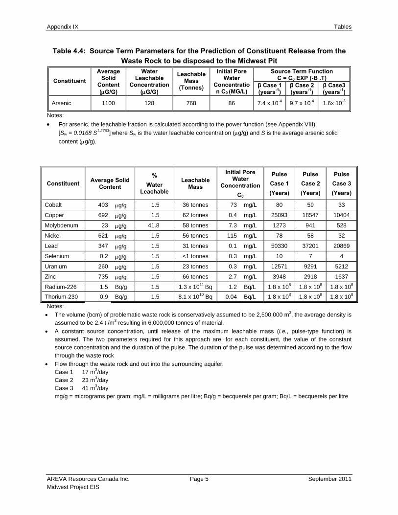
Appendix IX Tables


Table 4.4: Source Term Parameters for the Prediction of Constituent Release from the Waste Rock to be disposed to the Midwest Pit

Source Term Function C = C0 EXP (-Β .T) Constituent

Average Solid

Content (G/G)

Water Leachable

Concentration (G/G)

Leachable Mass

(Tonnes)

Initial Pore Water

Concentration C0 (MG/L)

β Case 1 (years-1)

β Case 2 (years-1)

β Case3 (years-1)

Arsenic 1100 128 768 86 7.4 x 10-4 9.7 x 10-4 1.6x 10-3

Notes:

For arsenic, the leachable fraction is calculated according to the power function (see Appendix VIII)

[Sw = 0.0168 S1.2763] where Sw is the water leachable concentration (g/g) and S is the average arsenic solid

content (g/g).

Constituent Average Solid

Content

%

Water Leachable

Leachable Mass

Initial Pore Water

Concentration

C0

Pulse

Case 1

(Years)

Pulse

Case 2

(Years)

Pulse

Case 3

(Years)

Cobalt 403 g/g 1.5 36 tonnes 73 mg/L 80 59 33

Copper 692 g/g 1.5 62 tonnes 0.4 mg/L 25093 18547 10404

Molybdenum 23 g/g 41.8 58 tonnes 7.3 mg/L 1273 941 528

Nickel 621 g/g 1.5 56 tonnes 115 mg/L 78 58 32

Lead 347 g/g 1.5 31 tonnes 0.1 mg/L 50330 37201 20869

Selenium 0.2 g/g 1.5 <1 tonnes 0.3 mg/L 10 7 4

Uranium 260 g/g 1.5 23 tonnes 0.3 mg/L 12571 9291 5212

Zinc 735 g/g 1.5 66 tonnes 2.7 mg/L 3948 2918 1637

Radium-226 1.5 Bq/g 1.5 1.3 x 1011 Bq 1.2 Bq/L 1.8 x 108 1.8 x 108 1.8 x 108

Thorium-230 0.9 Bq/g 1.5 8.1 x 1010 Bq 0.04 Bq/L 1.8 x 108 1.8 x 108 1.8 x 108

Notes:

The volume (bcm) of problematic waste rock is conservatively assumed to be 2,500,000 m3, the average density is assumed to be 2.4 t /m3 resulting in 6,000,000 tonnes of material.

A constant source concentration, until release of the maximum leachable mass (i.e., pulse-type function) is assumed. The two parameters required for this approach are, for each constituent, the value of the constant source concentration and the duration of the pulse. The duration of the pulse was determined according to the flow through the waste rock

Flow through the waste rock and out into the surrounding aquifer: Case 1 17 m3/day Case 2 23 m3/day Case 3 41 m3/day mg/g = micrograms per gram; mg/L = milligrams per litre; Bq/g = becquerels per gram; Bq/L = becquerels per litre

Appendix IX Tables


Table 4.5: Summary of Mass Transport Parameters Parameter Selected Value

Travel Distance (x)

From MODPATH model output

Calculated distances from the Midwest pit to Collins Creek area range from approximately 6,500 m to 8,100 with a mean distance of approximately 7,000 m.

Calculated distances from the Midwest pit to South McMahon Lake range from approximately 1,450 m to 1,600 with a mean distance of approximately 1,500 m.

Calculated distances from the Midwest pit to Shallow Lake range from approximately 2,000 m to 2,150 with a mean distance of approximately 2,080 m

Effective Porosity () 11% (COGEMA, 1997)

Pore water velocity (v)

From MODPATH model output (with = 11%)

Calculated velocities from the Midwest pit to Collins Creek area range from 0.05 m/year to 17 m/year with a mean pore water velocity of approximately 6 m/year for Case 3.

Calculated velocities from the Midwest pit to South McMahon Lake range from 1.2 m/year to 2.2 m/year with a mean pore water velocity of approximately 1.9 m/year for Case 2.

Calculated velocities from the Midwest pit to Shallow Lake range from 0.1 m/year to 0.5 m/year with a mean pore water velocity of approximately 0.3 m/year for Case 1.

Longitudinal dispersivity () 10% of the flow path distance ( = 0.1 * x), based on Gelhar et al., 1992

Distribution Coefficient (KD)

1 L/kg for As, Cu, Co, Ni, Mo, Pb, Se, Zn, U, Th

3.8 L/kg for Ra-226

No sorption for sulphate and chloride

Radioactive Decay Constant ()

226 Ra : 4.28 x 10-4 y-1 ( T½ = 1,620 years)

230 Th : 8.66 x 10-6 y-1 ( T½ = 8 x104 years)

210 Pb : 3.10 x 10-2 y-1 ( T½ = 22.3 years)

Table 4.6: Predicted Peak Incremental Loadings to South McMahon Lake and

Resulting Surface Water Concentrations Case 1 Case 2 Case 3

Constituents Mass Flux Concentration Mass Flux Concentration Mass Flux Concentration

Asa 1.7 x 10 0 8.6 x 10-1 3.6 x 10 0 1.8 x 10 0 0 0

Coa 6.2 x 10-2 3.1 x 10-2 1.7 x 10-1 8.4 x 10-2 0 0

Cua 2.2 x 10-2 1.1 x 10-2 1.2 x 10-1 5.8 x 10-2 0 0

Moa 9.6 x 10-2 4.7 x 10-2 2.7 x 10-1 1.3 x 10-1 0 0

Nia 9.5 x 10-2 4.7 x 10-2 2.6 x 10-1 1.3 x 10-1 0 0

Pba 5.6 x 10-3 2.8 x 10-3 2.9 x 10-2 1.4 x 10-2 0 0

Sea 1.7 x 10-4 8.6 x 10-5 6.4 x 10-4 3.2 x 10-4 0 0

Ua 1.7 x 10-2 8.3 x 10-3 8.5 x 10-2 4.2 x 10-2 0 0

Zna 9.9 x 10-2 4.9 x 10-2 3.1 x 10-1 1.5 x 10-1 0 0

Pb-210b 2.1 x 103 1.1 x 10-6 9.2 x 103 4.6 x 10-6 0 0

Ra-226b 1.0 x 100 4.8 x 10-10 6.1 x 101 3.1 x 10-8 0 0

Th-230b 1.8 x 102 8.7 x 10-8 1.3 x 103 6.5 x 10-7 0 0 a Mass Flux in kilograms per year – Concentration in micrograms per litre b Mass Flux in becquerels per year – Concentration in becquerels per litre

Appendix IX Tables



Case 1 Case 2 Case 3 Constituents

Mass Flux Concentration Mass Flux Concentration Mass Flux Concentration

Asa 1.4 x 10-6 1.6 x 10-6 3.0 x 10 0 3.2 x 10 0 0 0

Coa 1.2 x 10-7 1.3 x 10-7 1.4 x 10-1 1.5 x 10-1 0 0

Cua 6.9 x 10-9 7.5 x 10-9 9.4 x 10-2 1.1 x 10-1 0 0

Moa 1.1 x 10-7 1.1 x 10-7 2.2 x 10-1 2.4 x 10-1 0 0

Nia 1.8 x 10-7 2.0 x 10-7 2.2 x 10-1 2.4 x 10-1 0 0

Pba 1.7 x 10-9 1.9 x 10-9 2.4 x 10-1 2.6 x 10-2 0 0

Sea 3.4 x 10-10 3.7 x 10-10 5.3 x 10-4 5.8 x 10-4 0 0

Ua 5.1 x 10-9 5.6 x 10-9 6.9 x 10-2 7.6 x 10-2 0 0

Zna 4.6 x 10-8 5.1 x 10-8 2.5 x 10-1 2.7 x 10-1 0 0

Pb-210b 4.1 x 102 4.5 x 10-7 5.1 x 103 5.6 x 10-6 0 0

Ra-226b 1.7 x 10-9 1.8 x 10-18 2.1 x 101 2.2 x 10-8 0 0

Th-230b 1.6 x 10-5 1.7 x 10-14 6.9 x 102 7.5 x 10-7 0 0 a Mass Flux in kilograms per year – Concentration in micrograms per litre b Mass Flux in becquerels per year – Concentration in becquerels per litre


Case 1 Case 2 Case 3 Constituents

Mass Flux Concentration Mass Flux Concentration Mass Flux Concentration

Asa 1.8 x 10 0 4.1 x 10-2 6.6 x 10 0 1.5 x 10-1 7.9 x 10 1 1.8 x 10 0

Coa 6.6 x 10-2 1.5 x 10-3 1.7 x 10-1 3.9 x 10-3 3.8 x 10 0 8.7 x 10-2

Cua 2.3 x 10-2 5.2 x 10-4 1.2 x 10-1 2.7 x 10-3 4.4 x 10 0 1.0 x 10-1

Moa 1.0 x 10-1 2.3 x 10-3 2.7 x 10-1 6.2 x 10-3 6.0 x 10 0 1.4 x 10-1

Nia 1.0 x 10-1 2.3 x 10-3 2.6 x 10-1 6.1 x 10-3 5.8 x 10 0 1.3 x 10-1

Pba 5.7 x 10-3 1.3 x 10-4 2.9 x 10-2 6.7 x 10-4 1.2 x 10 0 2.6 x 10-2

Sea 1.8 x 10-4 4.2 x 10-6 6.5 x 10-4 1.5 x 10-5 2.6 x 10 0 5.9 x 10-4

Ua 1.7 x 10-2 3.9 x 10-4 6.5 x 10-4 2.0 x 10-3 2.1 x 10 0 4.9 x 10-4

Zna 1.1 x 10-1 2.3 x 10-3 8.5 x 10-2 7.1 x 10-3 6.7 x 10 0 1.6 x 10-1

Pb-210b 3.5 x 105 8.0 x 10-6 3.3 x 105 7.7 x 10-6 1.6 x 106 3.7 x 10-5

Ra-226b 1.0 x 100 2.3 x 10-11 6.1 x 101 1.4 x 10-9 6.8 x 105 1.6 x 10-5

Th-230b 2.2 x 102 5.1 x 10-9 1.3 x 103 3.1 x 10-8 4.6 x 105 1.1 x 10-5 a Mass Flux in kilograms per year – Concentration in micrograms per litre b Mass Flux in becquerels per year – Concentration in becquerels per litre

Appendix IX Tables


Table 5.1: Base Case versus Sensitivity Case – Summary of Source Term and Transport Parameters

Parameter Unit Base Case Sensitivity Analysis

Arsenic Leachable Mass Tonnes 768 2,318

Initial arsenic Pore Water Concentration

mg/L 86 115

Flow through the waste rock and out into the surrounding sandstone formation - Case 1 - Case 2 - Case 3

m3/day

17 23 41

21 27 48

Average groundwater velocity (Midwest Pit to Collins Creek) - Case 1 - Case 2 - Case 3

m/year

0.6 0.5 5.8

2.5 2.1

23.2

Collins Creek Flow m3/day 118,714 30,758

Shallow Lake Flow m3/dayb 2,506 1,382

South McMahon Lake m3/day 5,530 626

mg/L = micrograms per litre; m3/day = metres cubed per day; m/year = metres per year

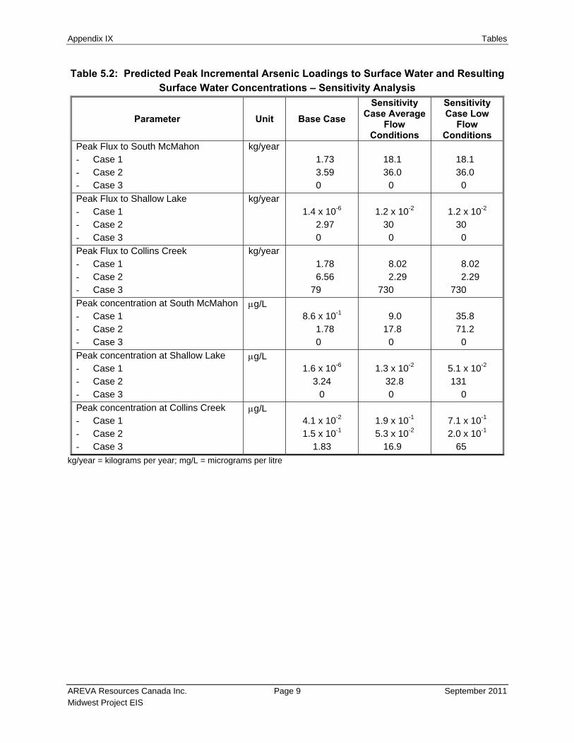
Appendix IX Tables


Table 5.2: Predicted Peak Incremental Arsenic Loadings to Surface Water and Resulting Surface Water Concentrations – Sensitivity Analysis

Parameter Unit Base Case

Sensitivity Case Average

Flow Conditions

Sensitivity Case Low

Flow Conditions

Peak Flux to South McMahon - Case 1 - Case 2 - Case 3

kg/year 1.73 3.59 0

18.1 36.0

0

18.1 36.0

0

Peak Flux to Shallow Lake - Case 1 - Case 2 - Case 3

kg/year 1.4 x 10-6

2.97 0

1.2 x 10-2

30 0

1.2 x 10-2

30 0

Peak Flux to Collins Creek - Case 1 - Case 2 - Case 3

kg/year 1.78 6.56

79

8.02 2.29

730

8.02 2.29

730

Peak concentration at South McMahon - Case 1 - Case 2 - Case 3

g/L 8.6 x 10-1

1.78 0

9.0

17.8 0

35.8 71.2

0

Peak concentration at Shallow Lake - Case 1 - Case 2 - Case 3

g/L 1.6 x 10-6

3.24 0

1.3 x 10-2

32.8 0

5.1 x 10-2

131 0

Peak concentration at Collins Creek - Case 1 - Case 2 - Case 3

g/L 4.1 x 10-2

1.5 x 10-1

1.83

1.9 x 10-1

5.3 x 10-2

16.9

7.1 x 10-1

2.0 x 10-1

65

kg/year = kilograms per year; mg/L = micrograms per litre

Appendix IX List of Figures

AREVA Resources Canada Inc. September 2011 Midwest Project EIS

LIST OF FIGURES




Figure 3.3: Simulated Steady-State Hydraulic Heads in the Lower Sandstone Midwest Pre-Mining Conditions

Figure 4.1: Steady-State Pathline Analysis - Post-Decommissioning Flow Regime

Figure 4.2: Pathline Analysis Cross Section between the Midwest Pit and Collins Creek - Post-Decommissioning Flow Regime

Figure 4.3: Midwest Pond Water Quality - Potential Arsenic Concentrations

Figure 4.4: Predicted Arsenic Loadings from Placed Waste Rock to Surface Water Receptors

Figure 4-6: Midwest Pond Water Quality – Potential Arsenic Concentrations

Figure 4-7: Predicted Arsenic Loadings from Placed Waste Rock to Surface Water Receptors – Base Case

Figure 4-7 Predicted Arsenic Loadings from Placed Waste Rock to Surface Water Receptors – Base Case

Figure 4.5: Predicted Arsenic Incremental Surface Water Concentrations

Figure 5.1: Sensitivity Analysis - Comparison between Realistic and Bounding Incremental Arsenic Loadings to Surface Water

Figure 5.2: Sensitivity Analysis - Predicted Arsenic Incremental Surface Water Concentrations

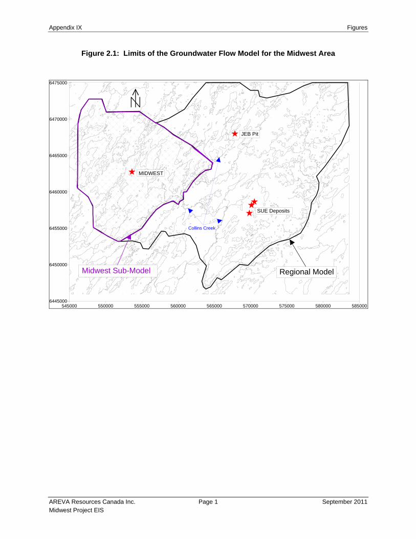
Appendix IX Figures



545000 550000 555000 560000 565000 570000 575000 580000 5850006445000

6450000

6455000

6460000

6465000

6470000

6475000

Midwest Sub-Model Regional Model

JEB Pit

MIDWEST

SUE Deposits

Collins Creek

Appendix IX Figures



Depth Interval Number of(m) Geo. Mean Minimum Maximum Measurements

0 to 50 1.0E-06 1.0E-09 4.0E-05 15150 to 124 4.9E-07 7.0E-09 8.0E-06 137124 to 190 1.8E-06 4.0E-09 2.0E-05 116190 to 240 2.3E-06 5.8E-08 2.0E-05 29

Hydraulic Conductivity (m/s)

0

5

10

15

20

25

1.0E

-09

2.5E

-09

5.0E

-09

7.5E

-09

1.0E

-08

2.5E

-08

5.0E

-08

7.5E

-08

1.0E

-07

2.5E

-07

5.0E

-07

7.5E

-07

1.0E

-06

2.5E

-06

5.0E

-06

7.5E

-06

1.0E

-05

2.5E

-05

5.0E

-05

>5.0

E-5

Hydraulic Conductivity (m/s)

Fre

quen

cy (

%)

Sandstone433 tests

Midwest - Sandstone - Packer Tests

1.E-09

1.E-08

1.E-07

1.E-06

1.E-05

1.E-04

0 20 40 60 80 100 120 140 160 180 200 220 240Depth (metres)

K (

m/s

)

Appendix IX Figures



Scalebar

0 50 100m

West East

Conglomerate

Orebody

Lines of equal hydraulic head

Direction of flow

OverburdenUpper Sandstone

Lower Sandstone

Basement

Appendix IX Figures


Figure 3.3: Simulated Steady-State Hydraulic Heads in the Lower Sandstone – Midwest Pre-Mining Conditions

Appendix IX Figures


Figure 4.1: Simulated Steady State Distribution of Hydraulic Heads in the Upper Sandstone Case 1 – Post-Decommissioning Conditions Flooded Pit – Plan View

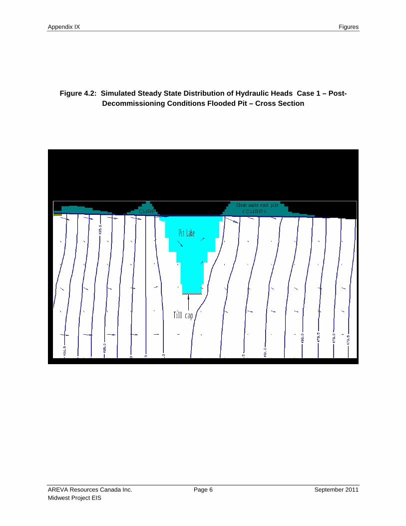
Appendix IX Figures


Figure 4.2: Simulated Steady State Distribution of Hydraulic Heads Case 1 – Post-Decommissioning Conditions Flooded Pit – Cross Section

Appendix IX Figures


Figure 4.3: Simulated Steady State Distribution of Hydraulic Heads in the Upper Sandstone Case 1 – Post-Decommissioning Conditions Fully Backfilled Option

Appendix IX Figures


Figure 4.4: Steady-State Pathline Analysis – Post Decommissioning Flow Regime

Case 1

Case 2

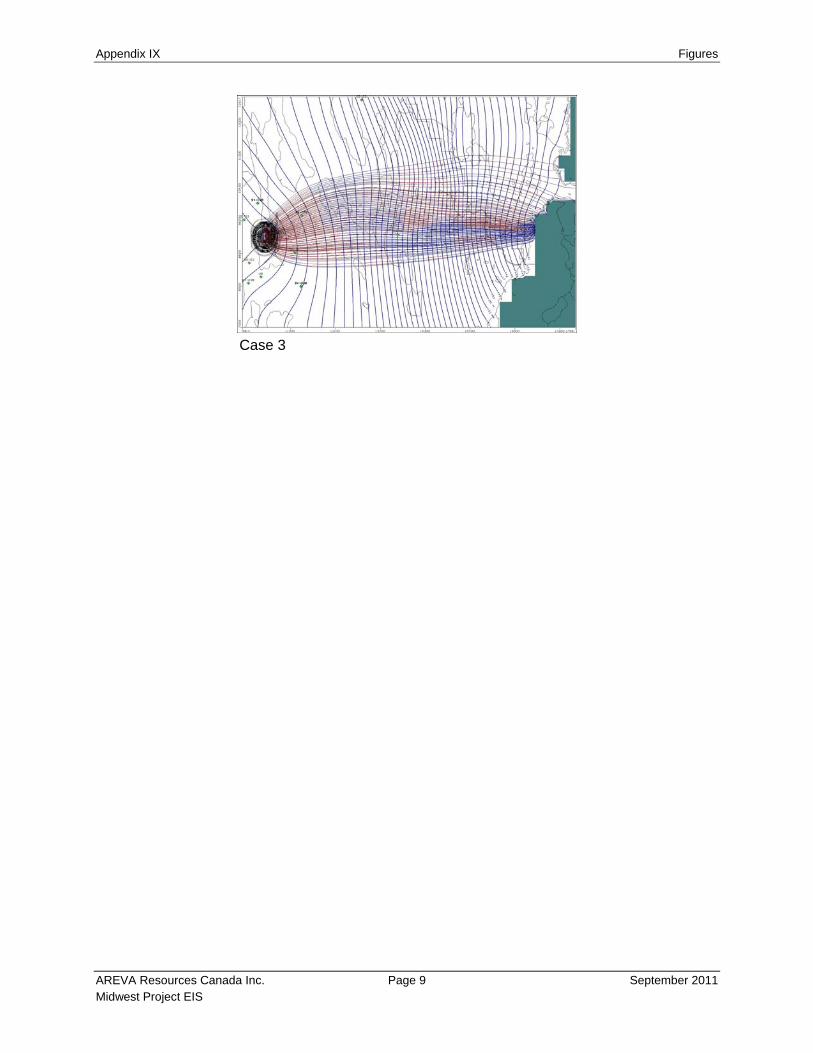
Appendix IX Figures


Case 3

Appendix IX Figures


Figure 4.5: Pathline Analysis – Cross Section between the Midwest Pit and Collins Creek – Post Decommissioning Flow Regime

Appendix IX Figures


Figure 4.6: Midwest Pond Water Quality – Potential Arsenic Concentrations

0

1

10

100

1000

1.0E-02 1.0E-01 1.0E+00Upward Flow (m3/day)

Ars

enic

(ug

/L)

D= 4.4e-10 m2/s

D = 1e-10 m2/s

D=5e-11 m2/s

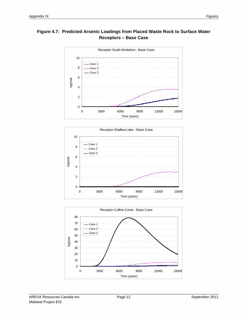
Appendix IX Figures


Figure 4.7: Predicted Arsenic Loadings from Placed Waste Rock to Surface Water Receptors – Base Case

Receptor South McMahon - Base Case

0

2

4

6

8

10

0 3000 6000 9000 12000 15000

Time (years)

kg/y

ear

Case 1

Case 2

Case 3

Receptor Shallow Lake - Base Case

0

2

4

6

8

10

0 3000 6000 9000 12000 15000

Time (years)

kg/y

ear

Case 1

Case 2

Case 3

Receptor Collins Creek - Base Case

0

10

20

30

40

50

60

70

80

0 3000 6000 9000 12000 15000

Time (years)

kg/y

ear

Case 1

Case 2

Case 3

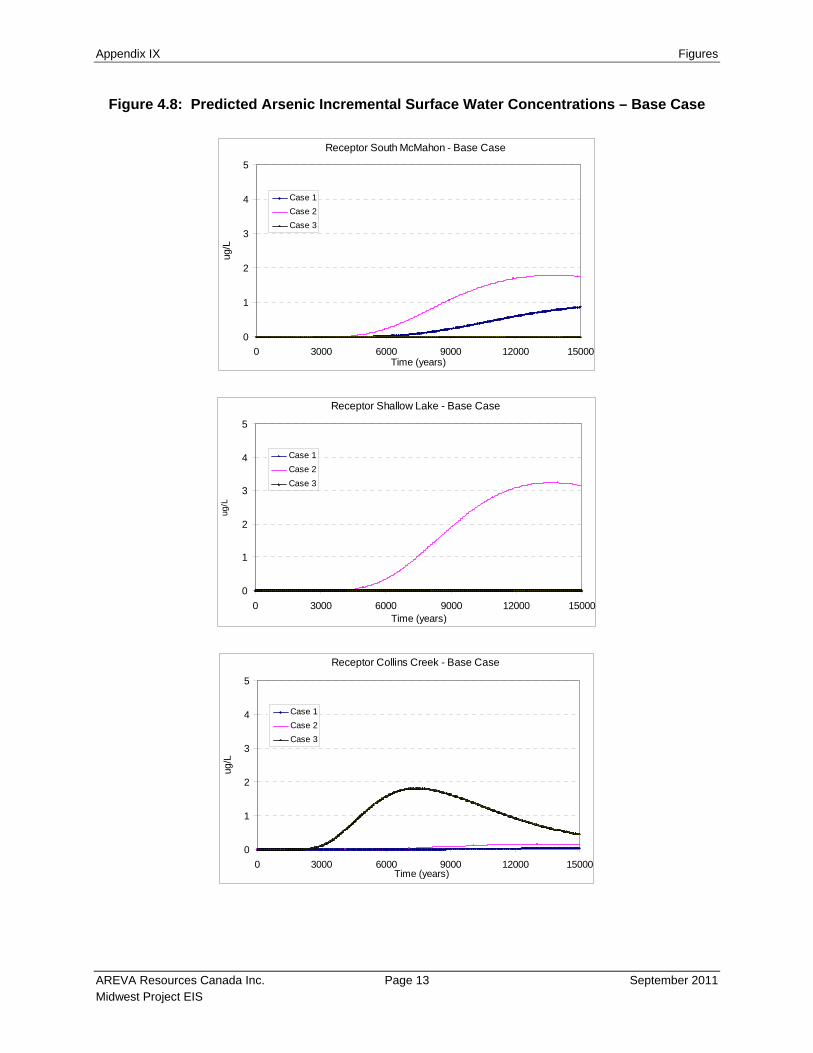
Appendix IX Figures


Figure 4.8: Predicted Arsenic Incremental Surface Water Concentrations – Base Case

Receptor South McMahon - Base Case

0

1

2

3

4

5

0 3000 6000 9000 12000 15000Time (years)

ug/L

Case 1

Case 2

Case 3

Receptor Shallow Lake - Base Case

0

1

2

3

4

5

0 3000 6000 9000 12000 15000Time (years)

ug/L

Case 1

Case 2

Case 3

Receptor Collins Creek - Base Case

0

1

2

3

4

5

0 3000 6000 9000 12000 15000Time (years)

ug/L

Case 1

Case 2

Case 3

Appendix IX Figures


Figure 5.1: Sensitivity Analysis – Predicted Arsenic Loadings from Placed Waste Rock to Surface Water Receptors

Receptor South McMahon - Sensitivity Case

0

10

20

30

40

0 2000 4000 6000 8000 10000

Time (years)

kg/y

ear

Case 1

Case 2

Case 3

Receptor Shallow Lake - Sensitivity Case

0

10

20

30

40

0 2000 4000 6000 8000 10000

Time (years)

kg/y

ear

Case 1

Case 2

Case 3

Receptor Collins Creek - Sensitivity Case

0

100

200

300

400

500

600

700

800

0 2000 4000 6000 8000 10000

Time (years)

kg/y

ear

Case 1

Case 2

Case 3

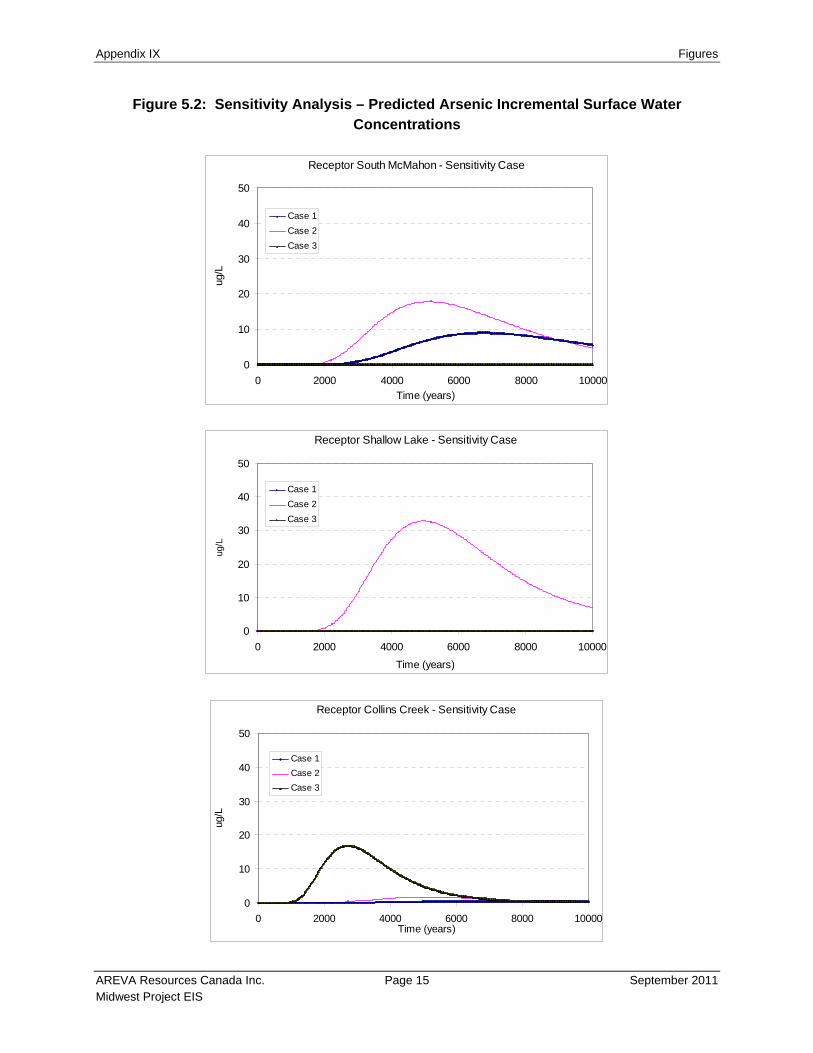
Appendix IX Figures


Figure 5.2: Sensitivity Analysis – Predicted Arsenic Incremental Surface Water Concentrations

Receptor South McMahon - Sensitivity Case

0

10

20

30

40

50

0 2000 4000 6000 8000 10000

Time (years)

ug/L

Case 1

Case 2

Case 3

Receptor Shallow Lake - Sensitivity Case

0

10

20

30

40

50

0 2000 4000 6000 8000 10000

Time (years)

ug/L

Case 1

Case 2

Case 3

Receptor Collins Creek - Sensitivity Case

0

10

20

30

40

50

0 2000 4000 6000 8000 10000Time (years)

ug/L

Case 1

Case 2

Case 3

waste rock management

Documents