watchdog sensor network with multi -stage rf signal ... · signal identification and cooperative...

Watchdog Sensor Network with Multi-Stage RF

Signal Identification and Cooperative Intrusion

Detection Xianbin Wang University of Western Ontario Jean-Yves Chouinard University of Laval Scientific authority: Rodney Howes DRDC Centre for Security Science The scientific or technical validity of the Contractor Report is entirely the responsibility of the Contractor and the contents do not necessarily have the approval or endorsement of Defence R&D Canada. Defence R&D Canada – Centre for Security Science Contract Report DRDC CSS CR 2012-007

March 2012

DRDC CSS CR 2012-007 i

Watchdog Sensor Network with Multi-Stage RF Signal

Identification and Cooperative Intrusion Detection Xianbin Wang University of Western Ontario Jean-Yves Chouinard University of Laval Scientific authority: Rodney Howes DRDC Centre for Security Science The scientific or technical validity of the Contractor Report is entirely the responsibility of the Contractor and the contents do not necessarily have the approval or endorsement of Defence R&D Canada.

Defence R&D Canada – Centre for Security Science Contract Report

DRDC CSS CR 2012-007 March 2012

DRDC CSS CR 2012-007 ii

Principal Author

Original signed by Xianbin Wang

Xianbin Wang University of Western Ontario

Approved by

Original signed by Rodney Howes

Rodney Howes DRDC Centre for Security Science, Project Manager

Approved for release by

Original signed by Dr. Mark Williamson

Mark Williamson DRDC Centre for Security Science, DRP Chair

© Her Majesty the Queen in Right of Canada, as represented by the Minister of National Defence, 2012

© Sa Majesté la Reine (en droit du Canada), telle que représentée par le ministre de la Défense nationale, 2012

DRDC CSS CR 2012-007 iii

Abstract The study report begins with an overview of existing wireless standards and signal sensing/identification technologies in the first section. The time/frequency/protocol features of each standard wireless signal are summarized. Our intent is to discover all inherent signal features for the development of multistage RF signal sensing/identification and cooperative intrusion detection. In section 2, the proposed multi-stage signal existence detection and identification techniques for watchdog sensor network are investigated for standard compatible wireless signals. To extend the study to non-standard signals, section 3 investigates blind transmission parameter detection for arbitrary communication signals, which are commonly used in military applications. In the final section, intrusion detection and physical layer authentication in mobile Ad Hoc networks and wireless sensor networks (WSNs) have been investigated. Résume Le rapport d’étude donne tout d’abord un aperçu des normes en vigueur dans le domaine du sans–fil et des techniques de détection/d’identification des signaux dans la première section. On donne un résumé des caractéristiques de protocole/fréquence/temps de chaque signal sans fil standard. Notre intention est de découvrir toutes les caractéristiques inhérentes des signaux pour mettre au point la détection d’intrusion en coopération et la détection/l’identification des signaux RF multi-étages. Dans la section 2, on étudie les techniques de détection et d’identification multi-étages de l’existence des signaux proposées pour le réseau WSN à l’égard des signaux sans fil compatibles standard. Pour étendre l’étude aux signaux non standard, on étudie à la section 3 la détection aléatoire des paramètres de transmission des signaux de communications arbitraires, qui servent couramment dans les applications militaires. Dans la dernière section, on examine la détection d’intrusion et l’authentification de la couche physique dans les réseaux ad hoc mobiles et les réseaux de capteurs sans fil.

DRDC CSS CR 2012-007 iv

Executive Summary

Due to the open nature of wireless communications, protection of critical wireless infrastructure from

malicious attacks has become increasingly important with the widespread deployment of various

wireless technologies and dramatic growth in user populations. This brings substantial technical

challenges to sensing and identification of various wireless signals using diverse transmission

technologies. Consequently, proper RF signal sensing, signal identification, data recovery, purpose

analysis and intrusion detection technologies are the essential steps to protect the wireless infrastructure

and improve its resilience to various attacks. The current PSTP study is dedicated to the development

of a software defined radio (SDR) based Watchdog Sensor Network (WSN) to enhance the security of

wireless communications based on the proposed novel multi-stage RF signal sensing, identification and

cooperative intrusion detection techniques. Each SDR sensor node is capable of identifying,

intercepting and analyzing any signal of interest, and reconfiguring its operating parameters depending

on the operational objectives of respective user groups. In addition, the proposed WSN will incorporate

multiple distributed SDR sensor nodes to achieve improved performance through cooperative

inspection and monitoring.

The study report begins with an overview of existing wireless standards and signal

sensing/identification technologies in the first section. The time/frequency/protocol features of each

standard wireless signal are summarized. Our intent is to discover all inherent signal features for the

development of multistage RF signal sensing/identification and cooperative intrusion detection.

Therefore, the focus of the standards survey is analyzing how and what type of wireless signals can be

detected and which unique features can be used to distinguish them from others. The comprehensive

standard survey covers the following wireless technologies from 2G to 4G: (a) IEEE 802.16 d and e

(WiMAX); (b) IEEE 802.11 (Wi-Fi) family of a, b, g, n, and s (c) Sensor networks based on IEEE

802.15.4: Wireless USB, Bluetooth, Wibree and Zigbee (d) 3G/4G cellular technologies: CDMA2000,

WCDMA, TD-SCDMA and LTE/HSPA+UMTS. Based on the extensive survey of various wireless

standards, signal sensing and identification techniques are overviewed and used as a starting point to

detect the existence of a wireless signal and estimate the corresponding parameters.

In section 2, the proposed multi-stage signal existence detection and identification techniques for

watchdog sensor network are investigated for standard compatible wireless signals. The proposed

signal existence detection and identification process consists signal existence detection, frequency

DRDC CSS CR 2012-007 v

range determination and signal identification. First, existence of an active signal of interest is

confirmed by energy of the received signal. Frequency range determination is then applied to the

received signals in order to limit the number of communication standards considered for the following

signal identification, since only a very few number of communication standards coexist in a specific

frequency range. Identification of a standard compliant signal is accomplished based on signal features

in both time and frequency domain in each communication standard. The proposed signal

identification for the watchdog sensor network covers the following most commonly used standards:

(a) cellular systems: GSM, IS-95, CDMA2000 and W-CDMA; (b) IEEE 802.11 (Wi-Fi) family of a, b,

g and n; (c) IEEE 802.116 (WiMAX); (e) IEEE 802.15.1 (Bluetooth); (f) IEEE 802.15.4.1 (Zigbee).

Theoretical analysis for signal detection, frequency range determination and signal identification, as

well as the related look-up table generation is provided in this section. Performances of the proposed

signal identification techniques are also evaluated through the analysis of signal identification error

probability and numerical simulations.

To extend the study to non-standard signals, section 3 investigates blind transmission parameter

detection for arbitrary communication signals, which are commonly used in military applications.

Without prior knowledge, estimation of the system parameters is a challenge in realistic scenarios with

low signal to noise ratio (SNR). In this section, a low-complexity sequential approach of blind system

parameters estimation and symbol recovery is proposed for Orthogonal Frequency Division

Multiplexing (OFDM) system, due to its popularity and wide use in broadband communciations.

Various algorithms for different blind parameters estimation of OFDM systems are studied. Moreover,

two new modulation classification algorithms are proposed for blind data recovery from the signal of

interest based on time-domain and frequency-domain features of the intercepted OFDM signals.

In the final section, intrusion detection and physical layer authentication in mobile Ad Hoc networks

and wireless sensor networks (WSNs) have been investigated. Since these networks do not have an

underlying infrastructure and the network topology is constantly changing, various potential security

vulnerabilities are introduced. This necessitates the need to constantly monitor the network status and

detect any suspicious behaviour. Intrusion detection systems are utilized for designing efficient

anomaly and intrusion behaviour detection through communication process monitoring and

engagement of proper countermeasures. An overview of the state of art technologies for intrusion

detection in wireless Ad Hoc networks and WSNs is presented in the beginning of the section. Based

on the technology survey, cross-layer based anomaly IDS is investigated to accommodate the integrated

property of routing protocols with link attributes in WSNs. This is motivated by exploiting the

DRDC CSS CR 2012-007 vi

cooperation from the physical layer, MAC layer and network layer of the WSNs to enhance network

behaviour monitoring from all the layers concurrently. Finally, a non-cryptographic physical layer

device identification scheme is proposed to enhance security by using the unique carrier frequency

offset (CFO) between each individual transmitter-receiver pair. This scheme uses the distinctive CFO

values as a transmitter-dependent signature for user identification and hence intrusion detection

purpose.

To validate all the proposed algorithms, a lab testing platform is set up to examine all the proposed

algorithms of signal existence detection, blind parameter estimation, modulation classification and data

recovery. The lab testing platform includes an arbitrary signal generator, a fading channel simulator,

and a high speed data acquisition system. Various tests are conducted to evaluate the performance of

the individual modules as well as the overall performance interception receiver. Numerical and lab

testing results on Wi-Fi signal show that the proposed algorithms are capable of achieving signal

detection and modulation classification in blind scenarios with very good performance. Based on the

numerical and lab test results, recommendations for choosing appropriate signal processing algorithms

in the watchdog sensor network are given to achieve the overall goal of security enhancement.

DRDC CSS CR 2012-007 vii

Sommaire En raison de la nature ouverte des communications sans fil, la protection de l’infrastructure sans fil

critique contre les attaques malveillantes prend de plus en plus d’importance dans le contexte du

déploiement généralisé des technologies sans fil et de l’augmentation spectaculaire des utilisateurs.

Cela pose de sérieux défis techniques à la détection et à l’identification des signaux sans fil qui font

appel à diverses techniques d’émission. C’est pourquoi les bonnes technologies de détection des

signaux RF, d’identification de ces signaux, de récupération des données, d’analyse du but et de

détection d’intrusion constituent les étages essentiels à la protection de l’infrastructure sans fil et à

l’amélioration de sa capacité de récupération suite à diverses attaques. L’étude en cours du PSTP porte

sur la mise au point d’un réseau de capteurs de surveillance (WSN) radio réalisé par logiciel (RRL)

dans le but de rehausser la sécurité des communications sans fil grâce aux techniques novatrices

proposées de détection des signaux RF en cascade, d’identification de ces signaux et de détection

d’intrusion en coopération. Chaque nœud de détection SDR peut identifier, intercepter et analyser tout

signal d’intérêt, puis reconfigurer ses paramètres de fonctionnement d’après les objectifs opérationnels

des groupes d’utilisateurs respectifs. En outre, le WSN proposé intégrera plusieurs nœuds de détection

SDR répartis en vue d’un meilleur rendement grâce à la surveillance et à l’inspection en coopération.

Le rapport d’étude donne tout d’abord un aperçu des normes en vigueur dans le domaine du sans–fil et

des techniques de détection/d’identification des signaux dans la première section. On donne un résumé

des caractéristiques de protocole/fréquence/temps de chaque signal sans fil standard. Notre intention est

de découvrir toutes les caractéristiques inhérentes des signaux pour mettre au point la détection

d’intrusion en coopération et la détection/l’identification des signaux RF multi-étages. Par conséquent,

la recherche sur les normes portera sur l’analyse des types de signaux sans fil susceptibles d’être

détectés, la façon dont ils peuvent être détectés et quelles caractéristiques uniques peuvent servir à les

distinguer les uns des autres. La recherche exhaustive sur les normes couvre les technologies 2G à 4G

suivantes : a) IEEE 802.16 d et e (WiMax); b) famille IEEE 802.11 a, b, g, n et s (Wi-Fi); c) réseaux de

détection fondés sur la norme IEEE 802.15.4 : USB sans fil, Bluetooth, Wibree et Zigbee; d)

technologies cellulaires 3G/4G : CDMA2000, WCDMA, TD-SCDMA et LTE/HSPA+UMTS. D’après

l’examen exhaustif des normes sans fil, les techniques de détection et d’identification des signaux sont

examinées et servent de point de départ de la détection de l’existence d’un signal sans fil et de

l’estimation des paramètres correspondants.

DRDC CSS CR 2012-007 viii

Dans la section 2, on étudie les techniques de détection et d’identification multi-étages de l’existence

des signaux proposées pour le réseau WSN à l’égard des signaux sans fil compatibles standard. Le

processus proposé de détection et d’identification de l’existence des signaux consiste en la détection de

l’existence des signaux, la détermination de la gamme de fréquences et l’identification des signaux.

Tout d’abord, l’existence d’un signal actif d’intérêt est confirmée par l’énergie du signal reçu. On

applique alors la détermination de la gamme de fréquences aux signaux reçus afin de limiter le nombre

de normes de communications considérées pour l’identification des signaux qui suivent, du fait que

seulement quelques normes de communications coexistent dans une gamme de fréquences donnée.

L’identification d’un signal conforme à une norme est accomplie d’après les caractéristiques du signal

dans les domaines du temps et des fréquences de chaque norme de communications. L’identification

des signaux proposée pour le réseau WSN couvre les normes les plus courantes qui suivent : a)

systèmes cellulaires : GSM, IS-95, CDMA2000 et W-CDMA; b) famille IEEE 802.11 a, b, g et n (Wi-

Fi); c) IEEE 802.116 (WiMax); e) IEEE 802.15.1 (Bluetooth); f) IEEE 802.15.4.1 (Zigbee). On

présente dans cette section l’analyse théorique en vue de la détection des signaux, de la détermination

de la gamme de fréquences et de l’identification des signaux, ainsi que de la génération de tables de

recherche connexes. Les rendements des techniques proposées d’identification des signaux sont aussi

évalués par l’analyse des simulations numériques et de la probabilité d’erreur d’identification des

signaux.

Pour étendre l’étude aux signaux non standard, on étudie à la section 3 la détection aléatoire des

paramètres de transmission des signaux de communications arbitraires, qui servent couramment dans

les applications militaires. Sans connaissance préalable, l’estimation des paramètres d’un système

constitue un défi dans des scénarios réalistes où le rapport signal/bruit (S/B) est faible. Dans cette

section, une approche séquentielle de faible complexité de l’estimation aléatoire des paramètres des

systèmes et de la récupération des symboles est proposée pour un système de multiplexage par

répartition orthogonale de la fréquence (MROF), en raison de sa popularité et de son usage courant

dans les communications à large bande. On étudie divers algorithmes en vue de l’estimation aléatoire

de différents paramètres des systèmes MROF. En outre, deux nouveaux algorithmes de classification de

modulation sont proposés pour la récupération aléatoire des données du signal d’intérêt d’après les

caractéristiques des domaines du temps et des fréquences des signaux MROF interceptés.

Dans la dernière section, on examine la détection d’intrusion et l’authentification de la couche physique

dans les réseaux ad hoc mobiles et les réseaux de capteurs sans fil. Comme ces réseaux n’ont pas

d’infrastructure sous-jacente et que leur topologie évolue constamment, on introduit diverses

DRDC CSS CR 2012-007 ix

vulnérabilités potentielles sur le plan de la sécurité. Cela nécessite le besoin de constamment surveiller

l’état des réseaux et de détecter tout comportement suspect. Les systèmes de détection d’intrusion

servent à la mise au point d’une détection efficiente du comportement des intrusions et des anomalies

grâce à la surveillance du processus de communications et à l’exécution de contre-mesures appropriées.

Un aperçu des techniques de détection d’intrusion de pointe dans les WSN et les réseaux ad hoc sans fil

est présenté au début de la section. D’après une étude des technologies, on examine les systèmes de

détection d’intrusion d’anomalies fondés sur le nappage pour tenir compte de la propriété intégrée des

protocoles de routage avec des attributs de liaison dans des WSN. C’est motivé par l’exploitation de la

coopération de la couche physique, de la couche MAC et de la couche réseau des WSN pour améliorer

la surveillance du comportement des réseaux à partir de toutes les couches en même temps. Enfin, on

propose un plan d’identification des dispositifs non cryptographiques de la couche physique pour

améliorer la sécurité en utilisant le décalage unique de la porteuse entre chaque paire individuelle

d’émetteur-récepteur. Ce plan utilise les valeurs distinctives du décalage de la porteuse comme une

signature dépendante de l’émetteur pour l’identification des utilisateurs et, par conséquent, aux fins de

la détection d’intrusion.

Pour valider tous les algorithmes proposés, on configure une plateforme d’essai de laboratoire pour

examiner tous les algorithmes proposés de détection de l’existence des signaux, d’estimation aléatoire

des paramètres, de classification des modulations et de récupération de données. La plateforme d’essai

de laboratoire comprend un générateur de signaux arbitraires, un simulateur de canal avec

évanouissement et un système d’acquisition de données haute vitesse. Divers essais sont menés en vue

de l’évaluation du rendement des modules individuels et du rendement global du récepteur

d’interception. Les résultats d’essais numériques et de laboratoire relatifs aux signaux Wi-Fi montrent

que les algorithmes proposés peuvent réaliser la détection de signaux et la classification des

modulations dans des scénarios aléatoires avec un très bon rendement. D’après les résultats d’essais

numériques et de laboratoire, on formule des recommandations pour choisir les algorithmes appropriés

de traitement des signaux dans le réseau WSN dans le but d’atteindre l’objectif global d’amélioration

de la sécurité.

DRDC CSS CR 2012-007 x

DRDC CSS CR 2012-007 1

Table of Contents Executive Summary ................................................................................................................................... iii Table of Contents ........................................................................................................................................ 1 Section 1 A Survey of Wireless Communication Standards and Signal Sensing / Identification Techniques 4

1.1 Introduction ....................................................................................................................................... 4 1.2 Communication Standards Survey .................................................................................................... 6 1.2.1 Second-generation (2G) Communication Standards ..................................................................... 6 1.2.2 Third-generation (3G) and Beyond 3G Standards ......................................................................... 9 1.2.2.1 CDMA2000............................................................................................................................... 10 1.2.2.2 WCDMA ................................................................................................................................... 12 1.2.2.3 TD-SCDMA .............................................................................................................................. 15 1.2.2.4 HSPA ......................................................................................................................................... 17 1.2.2.5 FLASH-OFDM ......................................................................................................................... 19 1.2.2.6 IEEE 802.16 .............................................................................................................................. 21 1.2.2.7 LTE ............................................................................................................................................ 24 1.2.3 IEEE 802.11 Wireless Local Area Network (WLAN) Standards ................................................ 28 1.2.4 Wireless Personal Area Network (WPAN) Standards .................................................................. 30 1.2.4.1 Bluetooth and IEEE 802.15.1 ................................................................................................... 31 1.2.4.2 Wibree (Bluetooth low energy) ................................................................................................. 35 1.2.4.3 Zigbee and IEEE 802.15.4 ........................................................................................................ 37 1.2.4.4 Wireless USB ............................................................................................................................ 40 1.2.4.5 UWB based WPAN ................................................................................................................... 41 1.3. Signal Sensing and Identification Techniques Survey ................................................................... 43 1.3.1 Signal Sensing Techniques Survey .............................................................................................. 44 1.3.1.1 Hypotheses for signal sensing ................................................................................................... 44 1.3.1.2 Signal Sensing Techniques ........................................................................................................ 45 1.3.2 Signal Match with Existing Communication Standards .............................................................. 51 1.3.3 Blind Estimation of Communication System Parameters ............................................................ 53 1.4 Conclusion ...................................................................................................................................... 54

Section 2 Multi-Stage Signal Detection and Identification in Watchdog Sensor Network ............... 55 2.1 Introduction ..................................................................................................................................... 55 2.2 Energy based Signal Existence Detection ....................................................................................... 58 2.2.1Detection Table Generation .......................................................................................................... 58 2.2.2Energy based Signal Existence Detection ..................................................................................... 58 2.2.2.1 Energy Detection Algorithm ..................................................................................................... 58 2.2.2.2 Threshold Selection .................................................................................................................. 60 2.2.3 Simulation Result ......................................................................................................................... 61 2.3 Frequency Range Determination .................................................................................................... 62 2.4 Feature Match based Signal Identification ..................................................................................... 63 2.4.1 746 MHz ~ 956 MHz Frequency Band ........................................................................................ 64 2.4.1.1 GSM (850MHz) ........................................................................................................................ 65 2.4.1.2 IS-95 /CDMA2000 (800MHz) .................................................................................................. 67 2.4.1.3 W-CDMA (850MHz) ................................................................................................................ 70 2.4.2 1.66 GHZ ~ 2.0 GHz Frequency Band ....................................................................................... 73 2.4.3 2.1 GHz Frequency Band ............................................................................................................ 73


2.4.4 2.3 GHz Frequency Band ............................................................................................................. 73 2.4.4.1 WiMAX (IEEE 802.16) ............................................................................................................ 73 2.4.5 2.4 GHz Frequency Band ............................................................................................................. 77 2.4.5.1 Wi-Fi (IEEE 802.11) ................................................................................................................. 77 2.4.5.2 Bluetooth (IEEE 802.15.1) ....................................................................................................... 87 2.4.5.3 Zigbee (IEEE 802.15.4) ............................................................................................................ 88 2.4.6 2.5 GHZ Frequency Band ........................................................................................................... 89 2.4.7 5 GHz ~ 6 GHz Frequency Band ................................................................................................ 89 2.4.7.1 IEEE 802.11a ............................................................................................................................ 90 2.4.7.2 IEEE 802.11n ............................................................................................................................ 90 2.4.8 Signal Identification Performance Evaluation ............................................................................ 90 2.5 Conclusion ...................................................................................................................................... 94

Section 3 Blind Parameter Estimation and Automatic Modulation Classification in Watchdog Sensor Network ......................................................................................................................................... 95

3.1. Introduction .................................................................................................................................... 95 3.2 Parameter Estimation of Unknown OFDM Signal ......................................................................... 98 3.2.1 Carrier Frequency Estimation ...................................................................................................... 98 3.2.2 Sampling Frequency Estimation .................................................................................................. 98 3.2.3 Number of Subcarriers Estimation............................................................................................... 99 3.2.4 Joint estimation of CP length, frequency and timing offset ....................................................... 101 3.3 Decision-Theoretic-based Automatic Modulation Classification ................................................. 102 3.3.1 ALRT-based Algorithms ............................................................................................................ 104 3.3.2. GLRT- and HLRT-based Algorithms ........................................................................................ 105 3.4 Pattern Recognition-based Automatic Modulation Classification ................................................ 106 3.4.1 Instantaneous Amplitude Phase and Frequency-based Algorithms ........................................... 106 3.4.2 Wavelet Transform-based Algorithms ....................................................................................... 107 3.4.3 Signal statistics-based Algorithms ............................................................................................. 108 3.5 Proposed Algorithms for AMC ......................................................................................................110 3.5.1 GMM-based Automatic Modulation Classification ....................................................................110 3.5.1.1 Gaussian Mixture Model..........................................................................................................110 3.5.1.2 Maximum Likelihood Parameter Estimation ...........................................................................113 3.5.1.3 Kolmogorov-Smirnov (K-S) Test ............................................................................................115 3.5.2 HOS-based Modulation Classification .......................................................................................116 3.5.2.1 Moments ..................................................................................................................................116 3.5.2.2 Cumulants ................................................................................................................................116 3.5.2.3 Proposed Modulation Classification Algorithm for OFDM Systems ......................................118 3.5.3 Performance Analysis of Data Recovery ....................................................................................119 3.6 Lab Testing Platform and Results ................................................................................................. 121 3.6.1 Hardware and Software Specifications ...................................................................................... 121 3.6.2 Equipment Interconnections and Setup ..................................................................................... 121 3.6.3 Signal Flow for Lab Testing ....................................................................................................... 123 3.6.3.1 Signal Generation.................................................................................................................... 124 3.6.3.2 Signal Reception ..................................................................................................................... 131 3.6.4 Evaluation for the Proposed Algorithms .................................................................................... 131 3.7. Conclusions and Future Work ...................................................................................................... 138

Section 4 Intrusion Detection and Physical Layer Authentication in Wireless Sensor Networks .. 140 4.1. Technical Background .................................................................................................................. 140 4.2. Introduction of Intrusion Detection Systems ............................................................................... 142


4.2.1. Information Sources for Intrusion Detection ............................................................................ 142 4.2.2. Intrusion Analysis ..................................................................................................................... 143 4.2.3. Responses to Detected Intrusions ............................................................................................. 148 4.3. Intrusion Detection in Ad Hoc Network ...................................................................................... 149 4.4.1. Physical-layer Intrusion Detection ............................................................................................ 152 4.4.1.1 RF Fingerprinting.................................................................................................................... 153 4.4.1.2 RF Features ............................................................................................................................. 153 4.4.1.2.1 Bi-Weight Scale (BWS) RF Feature Detection .................................................................... 154 4.4.2. MAC-layer Intrusion Detection ................................................................................................ 157 4.4.2.1 Impact of Interference on Misbehaviour Detection Schemes ................................................. 159 4.4.2.2 Proposed MAC-Layer Intrusion Detection ............................................................................. 161 4.4.3. Network-layer Intrusion Detection ........................................................................................... 165 4.4.3.1 Distributed IDS ....................................................................................................................... 166 4.4.3.2 Aodv Protocol-based IDS ....................................................................................................... 167 4.4.3.3 Techniques for Intrusion-resistant Ad Hoc Routing Algorithms ............................................ 168 4.4.3.4 Watchdog-pathrater Approach ................................................................................................ 169 4.5 Proposed Physical Layer Authentication Scheme......................................................................... 170 4.6 Conclusions ................................................................................................................................... 180

Appendix ................................................................................................................................................. 181 References ............................................................................................................................................... 183


Section 1 A Survey of Wireless Communication Standards and Signal Sensing / Identification Techniques

1.1 Introduction

Protection of critical wireless infrastructure has become increasingly important in recent years with the

widespread deployment of various wireless technologies and dramatic growth in user populations.

Wireless communication systems and networks suffer from various security threats, including attacks

similar to those in wired networks and those which are specific to the wireless environment. Wireless

communication signals are open to intrusion from the outside without the need for a physical connection

and, as a result, some techniques that would provide a high level of security in a wired network have

proven to be inadequate in wireless networks. This brings substantial technical challenges to the

spectrum regulation enforcement oriented signal sensing practice, due to the inherent difficulties in

obtaining the content, identification and network behaviour of a signal of interest through conventional

spectral analysis only.

The primary objective of this study is to further develop the necessary enabling technologies required to

protect the wireless infrastructure and improve its resilience to various attacks. Proper RF signal

sensing, signal identification, purpose analysis and intrusion detection are essential to protecting the

public against illegal usage of wireless communications and malicious attacks in addition to detecting

the presence of personal wireless devices in classified areas. Consequently, the project is dedicated to

the development of a software defined radio (SDR) based Watchdog Sensor Network (WSN) to enhance

the security of wireless communications based on novel multi-stage RF signal identification and

cooperative intrusion detection techniques. The proposed WSN will incorporate multiple distributed

SDR sensor nodes to achieve cooperative inspection and monitoring. Each SDR sensor node will be

capable of identifying, intercepting and analyzing any signal of interest, and reconfiguring its operating

parameters depending on the operational objectives of respective user groups.

Reliable signal sensing and identification techniques are fundamental to the proposed study on multi-

stage RF signal identification and cooperative intrusion detection. New techniques in this domain need

to be developed, while some existing signal sensing and identification techniques may be customized to

meet the specific purposes of this study.


Some of the relevant signal detection and identification techniques are originated from Software Defined

Radio, where initial transmission mode identification has to be performed over a large span of the

potential frequency spectrum to identify the user air interface. Once a communication link is established,

an SDR has to monitor alternative air interfaces to be able to perform inter-standard handover if

necessary. To be specific, the signal detection could be realized through signal sensing and

identifications, which are widely used in cognitive radio communications. Signal sensing provides the

capability to sense, learn, and discover the parameters related to the radio channel characteristics,

availability of spectrum and operating environment, user requirements and applications, and network

availability (infrastructures).

The proposed multi-stage RF signal identification starts with energy based signal sensing. After

confirmation of the existence of an active radio signal, the next step is to identify the time and frequency

domain features of the standard compatible signals, or determine the transmission parameters of the

received signal through blind estimation techniques, when the received signal is transmitted with non-

standard user-defined format. In this case, the SDR has to perform the following tasks to analyze the

received wideband signal.

o Estimate the carrier frequency and bandwidth.

o Determine the related air interfaces in the radio frequency band.

o Identification of specific air interface.

In this survey, we focus primarily on summarizing the key features of different communication

standards. Many modulation classification algorithms have been developed for both civilian and defence

communications. However, most of these algorithms are based on the assumption that there is only one

modulated signal from one particular user in the channel at a given time. While this assumption may be

true for TDMA based signals, it does not hold for CDMA signals, where the signals of individual users

interfere with each other in time and frequency, and for OFDM signals, where the symbols of one single

user is transmitted in parallel over multiple carriers, which overlap in the frequency domain. Hence,

conventional modulation recognition algorithms cannot be used to recognize CDMA and OFDM based

air interfaces, which constitute the majority of the newer generation wireless communication systems.

Therefore, one purpose of this section is to analyze how and what type of wireless signal features can be

used for signal detection and identification. A second purpose is to generalize the specific signal and

protocol features of different systems for the development network behaviour analysis and intrusion

detection at higher link layers. Various wireless standards, including Wireless Local Area Networks


(WLANs) and Wireless Personal Area Networks (WPANs) are covered. In addition, popular signal

sensing and detection techniques are also summarized to develop a generic signal identification method.

1.2 Communication Standards Survey

The rapid increase in the number of wireless mobile subscribers, which currently exceeds 3 billion users

worldwide, indicates the importance of wireless communications nowadays. This revolution in

communication technologies has taken place, especially in North America and Europe through a

continuous evolution of wireless communications standards and applications by keeping a seamless

strategy for the choice of solutions and parameters. The continuous adaption of wireless technologies to

meet the users’ rapidly increasing demands is and will continue to be characterized by a heterogeneous

multitude of standards and systems.

This plethora of wireless communication standards and applications is not limited to cellular mobile

telecommunication systems such as Global System for Mobile Communications (GSM), IS-95, PDC,

CDMA2000, WCDMA/UMTS, HSPA and 3GPP LTE, but also includes wireless metropolitan area

networks (WMAN) and local area networks (WLANs), e.g. WiMAX IEEE 802.16x, IEEE 802.11

a/b/g/n, and Bluetooth. These trends have accelerated since the beginning of the 1990s with the

replacement of the first-generation analogue mobile networks by the current second-generation (2G)

systems (GSM, IS-95, D-AMPS, and PDC), which opened the door for fully digital networks. This

evolution is continuing with the deployment of the third-generation (3G) systems namely

WCDMA/UMTS, HSPA, and CDMA-2000, referred to as IMT2000. The 3GPP Long Term Evolution

(LTE) standard with significantly higher data rates than in 3G systems can be considered as 3G

evolution. In the meantime, the research community is focusing its activity towards the next-generation

(4G) systems, with even more ambitious communication capacity and technological challenges.

Therefore, in this survey, we follow the technology evolution path from 2G to 4G, and for each

generation we analyzed the primary standards involved and compared the corresponding features which

can be used for the following sections, i.e., signal sensing and identification, user behaviour analysis and

intrusion detection.

1.2.1 Second-generation (2G) Communication Standards

The 2G wireless systems are mainly characterized by the transition from analogue to a fully digital


technology and comprise several different standards such as GSM, IS-95 and PDC standards.

Research and development work on GSM started in 1982 [1,2], where it now accounts for about 85% of

the global mobile market. This standard was approved by the European Telecommunications Standards

Institute (ETSI), where its commercial success began in 1993. Although GSM is optimized for circuit-

switched services such as voice, it offers low rate data services up to 14.4 kbit/s. High speed data

services with up to 171.2 kbit/s are possible with the enhancement of the GSM standard, namely the

General Packet Radio Service (GPRS), by assigning multiple time slots to one link. GPRS uses the same

modulation, frequency band, and frame structure as GSM. The Enhanced Data Rate for Global

Evolution (EDGE) [3] system, which further improves the data rate up to 384 kbit/s, introduces a new

spectrum efficient modulation scheme. Parallel to GSM, the American IS-95 standard [4] (recently

renamed CDMAOne) was approved by the Telecommunication Industry Association (TIA) in 1993. The

first convincing example of high speed mobile internet services, called i-mode, was introduced in 1999

in Japan in the Personal Digital Cellular (PDC) system.


The following table describes the main parameters of 2G mobile radio systems:

Parameter 2G systems

GSM (GPRS, EDGE) IS-95/CDMAOne PDC

Carrier Frequencies 900 MHz

1800 MHz

850 MHz

1900 MHz

850 MHz

1500 MHz

Peak Data Rate 64 kbit/s

171.2 kbit/s (GPRS)

384 kbits/s (EDGE)

64 kbit/s

144 kbit/s

28.8 kbit/s

Multiple Access TDMA CDMA TDMA

Services Voice, low data rate Voice, low data rate Voice, low data rate

Channel Bandwidth 200 kHz 1250 kHz 30 kHz

Number of duplex

channels 125 832 20

Modulation GMSK QPSK π/4 DQPSK

Carrier Bit Rate 270.8 kbps 9.6 kbps 48.6 kbps

Table 1.1. Main transmission parameters of 2G mobile radio systems.

Based on the system parameters above, the detection of a 2G signal could utilize the carrier frequency

information to narrow down the possibility of either a GSM, cdmaOne or PDC signal. Further

identification can then be realized through specific spectrum features such as the different channel

bandwidth used by each standard. In addition, from the protocol level, the three systems all have

different frame structures which can be used as the second level parameters for identification. For

example, the hierarchical frame structure of the GSM system is depicted as follows:


Figure 1.1. GSM Frame Structure.

As shown in Figure 1.1, each timeslot (TS) has a duration of 577 microseconds (μsec), eight timeslots

compose a frame and 26 frames compose a multiframe. GSM is essentially a time division multiple

access (TDMA) system, rather than a spread spectrum system. With guard times of 8.25 μsec at the end

of each timeslot, a timeslot carries 148 usable bits of information; 114 of these are the message payload,

the remaining 26 bits are training bits for frame synchronization, 6 start/stop bits, and 2 “stealing bits”

for inserting priority control messages. For all the physical channels being used, control channels are

located on 34 designated carrier frequencies; that is, 34 out of 1000 physical channels are reserved for

paging and broadcast, frequency correction, and timing synchronization. Some of these are for the

handshaking process to initiate calls, and granting access to a regular traffic channel. Several others are

holding channels, to maintain a connection while the setup process is underway. Traffic channels are of

various rates, according to the perceived need.

1.2.2 Third-generation (3G) and Beyond 3G Standards

Technology evolution towards improved capacity, new multimedia services, and new frequencies has

DRDC CSS CR 2012-007 10

motivated the development of 3G systems. A unique international standard was targeted, referred to as

International Mobile Telecommunications 2000 (IMT-2000), realizing a new generation of mobile

communications technology, namely WCDMA/UMTS, HSPA, and CDMA-2000, which went far

beyond the second-generation systems, especially with respect to:

o The wide range of multimedia services (speech, audio, image, video, data) and bit rates (up to

14.4 Mbit/s for indoor and hot spot application);

o The high quality of service requirements (better speech/image quality, lower bit error rate, higher

number of active users);

o Flexibility in frequency (variable bandwidth), in data rate (variable), and in radio resource

management (variable power/channel allocation)

Similar to the survey of 2G communication systems, key features of each 3G standard need to be

specified for signal sensing identification purpose. The unique challenge is due to the variation of

transmission technologies used in 3G standards from CDMA and OFDM to OFDMA. As a result, one

important step is to classify single carrier and multi-carrier modulated signals. Based on this, other

signal parameters/features can be identified to achieve our eventual goal.

1.2.2.1 CDMA2000

CDMA2000, also known as IMT Multi-Carrier (IMT-MC), is a family of 3G mobile technology

standards which use code-division channel to send voice, data and signalling between mobile phones

and cell sites. CDMA2000 1X (IS-2000), also known as 1xRTT, is the core of the CDMA2000 wireless

air interface standard. The designation "1x" means one times Radio Transmission Technology, which

uses the same RF bandwidth as IS-95. However, 1xRTT almost doubles the capacity of IS-95 by adding

64 more traffic channels to the forward link, orthogonal to (in quadrature with) the original set of 64.

IMT-2000 also made changes to the data link layer for the greater use of data services, including

medium and link access control protocols and QoS.

DRDC CSS CR 2012-007 11

The following table summarizes the key parameters in CDMA2000 standards:

Frequencies 450, 850, 900 MHz 1.7, 1.8, 1.9, and 2.1 GHz

Spectrum Type Licensed (Cellular/PCS/3G/AWS)

Channel bandwidth 1.25, 5, 10, 15, 20 MHz

Downlink RF channel structure

Direct spread or multicarrier

Chip rate n x 1.2288 Mc/s (n = 1 , 3, 6, 9, 12) Frame length 20 ms for data and control/5 ms for control information on the fundamental and

dedicated control channel Spreading modulation Balanced OPSK (down link)

Dual channel OPSK (uplink) Complex Spreading Circuit

Data modulation OPSK (downlink) BPSK (uplink)

Coherent detection Pilot time multiplexed with PC and EIB (uplink) Common continuous pilot channel and auxiliary pilot (downlink)

Channel multiplexing in uplink

Control, pilot. fundamental, and supplemental code multiplexed I/O multiplexing for data and control channels

Multirate Variable spreading and multicode Spreading (downlink) Variable length Walsh sequences for channel separation, M-sequence 215

(same sequence with different time shifts utilized in different cells, different sequence in I/O channel)

Spreading (uplink) Variable length orthogonal sequences for channel separation, M-sequence 215

(same sequence for all users, different sequences in I/O channels); M-sequence 241− 1 for user separation (different time shifts for different users)

Table 1.2. Summary of CDMA2000 system parameters.

Different types of transmission channels can be used to characterize CDMA2000 standards. To be

specific, there are four different dedicated channels in the uplink. The fundamental and supplemental

channels carry user data. A dedicated control channel, with a frame length 5 or 20 ms, carries control

information, and a pilot channel is used as a reference signal for coherent detection. The pilot channel

also carries time multiplexed power control symbols [5]. The reverse access channel (R-ACH) and the

reverse common control channel (R-CCCH) are common channels used for communication of layer 3

and MAC layer messages. The R-ACH is used for initial access, while the R-CCCH is used for fast

packet access.

DRDC CSS CR 2012-007 12

Alternatively, the downlink has three different dedicated channels and three common control channels.

Similar to the uplink, the fundamental and supplemental channels carry user data and the dedicated

control channel control messages. The dedicated control channel contains power control bits and rate

information. The synchronization channel is used by the mobile stations to acquire initial time

synchronization. One or more paging channels are used for paging the mobiles. The pilot channel

provides a reference signal for coherent detection, cell acquisition, and handover. In the downlink,

CDMA2000 has a common pilot channel, which is used as a reference signal for coherent detection

when adaptive antennas are not employed.

1.2.2.2 WCDMA

The WCDMA scheme has been developed as a joint effort between ETSI and ARIB during the second

half of year 1997 [6]. The ETSI WCDMA scheme has been developed from the FMA2 scheme in

Europe [7-9] and the ARIB WCDMA was from the Core-A scheme in Japan [10-12]. The uplink of the

WCDMA scheme is based mainly on the FMA2 scheme, and the downlink on the Core-A scheme,

which is a unique feature for WCDMA. In this section, we present the main technical features of the

ARIB/ETSI WCDMA scheme. Table 1.3 lists the main parameters of WCDMA.

Carrier spacing and Deployment Scenarios

The carrier spacing has a raster of 200 kHz and can vary from 4.2 to 5.4 MHz. Different carrier spacing

can be used to obtain suitable adjacent channel protection depending on the interference scenario. Fig.

1.2 shows an example for the operator bandwidth of 15 MHz with three cell layers. Larger carrier

spacing can be applied between operators in order to avoid inter-operator interference.

DRDC CSS CR 2012-007 13

Frequencies 850 MHz, 1.9, 1.9/2.1, and 1.7/2.1 GHz

Spectrum Type Licensed (Cellular/PCS/3G/AWS)

Channel bandwidth 1.25, 5, 10, 15, 20 MHz

Chip rate 1 .024 /4.096/ 8.192/1 6.384 Mc/s Roll off factor 0.22 Frame length 10 ms/20 ms (optional) Spreading modulation Balanced OPSK (down link)

Dual channel OPSK (uplink) Complex Spreading Circuit

Data modulation OPSK (downlink) BPSK (uplink)

Coherent detection User dedicated time multiplexed pilot(downlink and uplink); no common pilot in downlink

Channel multiplexing in uplink Control, pilot, fundamental, and supplemental code multiplexed I&O multiplexing for data and control channels

Multirate Variable spreading and multicode

Table 1.3. Summary of WCDMA parameters.

Figure 1.2. Frequency utilization with WCDMA.

Physical Channels of WCDMA

There are two dedicated channels and one common channel on the uplink. User data is transmitted on

the dedicated physical data channel (DPDCH), and control information is transmitted on the dedicated

physical control channel (DPCCH). Fig. 1.3 shows the principle frame structure of the uplink DPDCH

DRDC CSS CR 2012-007 14

and DPCCH. The overall DPDCH bit rate is variable on a frame-by-frame basis.

Figure 1.3. WCDMA uplink multirate transmission.

In most cases, only one DPDCH is allocated per connection, and services are jointly interleaved sharing

the same DPDCH. However, multiple DPDCHs could also be allocated. The dedicated physical control

channel (DPCCH) is needed to transmit pilot symbols for coherent reception, power control signalling

bits, and rate information for rate detection. Two basic solutions for multiplexing physical control and

data channels are time multiplexing and code multiplexing. A combined I/Q and code multiplexing

solution (dual-channel QPSK) is used in WCDMA uplink to avoid electromagnetic compatibility (EMC)

problems with discontinuous transmission (DTX).

For the downlink, there are three common physical channels. The primary and secondary common

control physical channels (CCPCH) carry the downlink common control logical channels (BCCH, PCH,

and FACH); the SCH provides timing information and is used for handover measurements by the mobile

station. The dedicated channels (DPDCH and DPCCH) are time multiplexed. Also, time multiplexed

pilot symbols are used for coherent detection. Since the pilot symbols are known to the receiver, they

can be used for channel estimation with adaptive antennas as well. Furthermore, the connection

dedicated pilot symbols can be used to support downlink fast power control. In addition, a common pilot

time multiplexed in the BCCH channel can be used for coherent detection.

Multi-rate Supporting Mechanism

Multiple services of the same connection are multiplexed on one DPDCH. Multiplexing may take place

either before or after the inner or outer channel coding. After service multiplexing and channel coding,

DRDC CSS CR 2012-007 15

the multiservice data stream is mapped to one DPDCH. If the total rate exceeds the upper limit for single

code transmission, several DPDCHs can be allocated. A second alternative for service multiplexing

would be to map parallel services to different DPDCHs in a multi-code fashion with separate channel

coding/interleaving. With this alternative scheme, the power and the quality of each service can be

separately and independently controlled. The disadvantage is the need for multicode transmission, which

will have an impact on mobile station complexity. Multicode transmission sets higher requirements for

the power amplifier linearity in transmission, and more correlators are needed for reception.

1.2.2.3 TD-SCDMA

While WCDMA supports both FDD and TDD, TD-SCDMA uses only a TDD (Time Division

Duplexing) scheme. Both WCDMA and TC-SCDMA use the same channel for uplink and downlink and

use the same signal spreading method, however, the signalling in TD-SCDMA is controlled by time

division. TD-SCDMA uses a chip-rate of 1.28 Mcps (Mega chips per second), and is therefore referred

to as Low Chip Rate TDD (LCR TDD) by the 3GPP [13]. TD-SCDMA operates without the needs of a

paired spectrum (TDD unpaired band) and works well with asymmetric traffic [13]. As shown in Figure

1.4, the advantage of working without the need for a paired spectrum is that it requires a smaller

bandwidth and better utilization of the spectrum in asymmetric services. TD-SCDMA is also able to

cover large areas, up to 40 km [14], and supports high mobility. The symmetric service consists of

speech and video traffic, and the asymmetric traffic is mainly mobile internet traffic.

DRDC CSS CR 2012-007 16

Figure 1.4. TD-SCDMA unpaired spectrum.

Several special techniques introduced in TD-SCDMA can be utilized to differentiate it from other

standards. The following are a few features that differentiate TC-SCDMA from other standards.

o Smart Antennas - The idea behind Smart Antennas (SA) is to distribute the power to the part of

the cell that contains mobile subscribers, i.e. active terminals. Without SA, transmitted power

spreads over the whole cell, thus creating interference between cells. The SAs contain a

concentric array of eight antenna elements located in the TD-SCDMA base station and track

mobile terminals throughout the cell. This can reduce the number of base stations in densely

populated urban areas. It can also reduce the number of base stations in rural areas with low

population density. This is mainly due to the fact that more power can be directed in a particular

direction [13].

o Joint Detection - Another feature of the TD-SCDMA technique is Joint Detection (JD). This

technique is used to combat the Multiple Access Interference (MAI) experienced in other CDMA

systems. Signals from mobile devices received at base stations are affected by multipath

propagation caused by reflections, diffractions, and attenuation of the signal from buildings,

hills, and so on. This results in the same signal arriving from different paths to the base station,

but they are slightly out of sync. The signals will then combine constructively and destructively.

In addition, signals from different terminals can also interfere with each other, adding to the

challenge of successfully recovering the signal. With a Joint Detection Unit the effect of this

phenomenon can be minimized.

DRDC CSS CR 2012-007 17

o Terminal Synchronization - Terminal Synchronization (TS) is used for tuning the transmission

timing of each mobile terminal with respect to its base station. This way the quality of the uplink

signal can be improved. The localization of a terminal can be made easier and thus lead to more

simple handovers. The TS also eliminates the need for soft handovers in the system [13].

Table 4 summarizes the basic parameters used in TD-SCDMA systems.

Frequencies 450, 850 MHz, 1.9, 2, 2.5, and 3.5 GHz Spectrum Type Licensed (Cellular, 3G TDD, BRS/IMT-ext, FWA) Minimum frequency band required 1.6MHz Frequency re-use 1(or 3) Duplex type TDD Chip rate 1.28 Mc/s Frame length [ms] 10 Modulation QPSK or 8-PSK Receiver Joint Detection Power control period 200 Hz Handovers Hard, Baton Physical layer spreading factors 1, 2, 4, 8, 16

Table 1.4. Summary of TD-SCDMA parameters.

1.2.2.4 HSPA

High Speed Packet Access (HSPA) [15] is an amalgamation of two mobile telephony protocols, High

Speed Downlink Packet Access (HSDPA) and High Speed Uplink Packet Access (HSUPA). It extends

and improves the performance of existing WCDMA protocols. Another standard named Evolved HSPA

(also known as HSPA+), was released in late 2008 with subsequent adoption worldwide beginning in

2010. The features of the two protocols are explained and summarized below.

HSDPA Overview

HSDPA has been designed to support peak data rates of 14.4 Mbps in one cell. The major enhancement

is the introduction of a new transport channel known as HS-DSCH [16], plus two control channels for

the uplink and downlink. It is a shared channel which can be used by several users simultaneously. The

introduction of this new transport channel impacts several protocol layers; the most significant changes

DRDC CSS CR 2012-007 18

are in the physical and MAC layers.

The following features enable the high throughput capabilities of HSDPA:

o HSDPA introduces an Adaptive Modulation and Coding (AMC) scheme, whereby modulation

method and coding rate are selected based on channel state information provided by the terminal

and the Node-B. In the downlink, HSDPA supports 16-QAM as a higher-order modulation

method for data transmission under good channel conditions.

o MAC Protocol Enhancements - HSDPA not only introduces new transport and physical layer

channels, but also has an impact on higher-layer protocols, including the MAC layer. Different

types of MAC entities are identified for different classes of transport channels. In 3GPP Rel. 99,

dedicated and common transport channels are differentiated, and consequently, the MAC layer

contains a MAC-d and a MAC-c entity.

o Control Plane Protocols - The introduction of HSDPA also requires additions and modifications

to control plane protocols used within the access network, i.e. specifically the Radio Resource

Control (RRC) protocol and the Node-B Application Part (NBAP) protocol. Since these protocol

modifications are irrelevant to signal sensing and identification at the physical layer, they are not

discussed in this report.

HSUPA Overview

The goal of HSUPA is to improve capacity and data throughput and reduce the delays in dedicated

channels in the uplink. The main enhancement offered by the 3GPP specifications is the definition of a

new transport channel denoted as E-DCH (Enhanced Dedicated Channel). The maximum theoretical

uplink data rate that can be achieved is 5.6 Mbps. As with HSDPA, E-DCH relies on improvements

implemented in both the PHY and the MAC layer. However, one difference is that HSUPA does not

introduce a new modulation scheme; instead it relies on the use of QPSK.

DRDC CSS CR 2012-007 19

Parameters HSDPA HSUPA Peak Data Rate 14.4 Mbps 5.6 Mbps Modulation Scheme(s) QPSK, 16QAM QPSK Transmission time interval (TTI) 2 ms 2 ms(optional)/10 ms Transport Channel Type Shared Dedicated Adaptive Modulation and Coding Yes No HARQ HARQ with incremental redundancy (IR) HARQ with IR Packet Scheduling Downlink Scheduling

(for capacity allocation) Uplink Scheduling (for power control)

Soft Handover Support No (in the Downlink) Yes

Table 1.5. Feature comparison between HSDPA and HSUPA.

At the physical layer, E-DCH introduces five new physical layer channels [17]. Just as with HSDPA, the

Node-B contains an uplink scheduler for HSUPA. However, the goal of the scheduling operation is

completely different compared with that of HSDPA. The aim of HSDPA is to allocate HS-DSCH

resources (in terms of time slots and codes) to multiple users, the goal of the uplink scheduler is to

allocate only as much capacity to the individual E-DCH users as is necessary to ensure that Node-B does

not have a “power-overload”. In addition to introducing new physical channels, E-DCH also introduces

new MAC entities for the UE, the Node-B and the SRNC. The details of these modifications in MAC

layer are not discussed. Table 1.5 gives a comparison of significant similarities and differences between

HSDPA and HSUPA.

1.2.2.5 FLASH-OFDM

Fast Low-latency Access with Seamless Handoff Orthogonal Frequency Division Multiplexing

(FLASH-OFDM), is a system based on OFDM which also specifies higher layer protocols. It has been

developed and is marketed by Flarion. Flash-OFDM has generated interest as a packet-switched cellular

bearer, where it would compete with GSM and 3G networks.

From the physical layer, the features of F-OFDM standard can be defined as:

o Transmission Scheme - The transmission technique used by FLASH-OFDM is based on a fast

tone hopping scheme. In this scheme, users are allocated to OFDM subcarriers (tones) according

DRDC CSS CR 2012-007 20

to a pseudorandom predetermined hopping pattern. This hopping pattern ensures that users

within the same cell are allocated orthogonal resources and use a different subcarrier for each

symbol in downlink and every 7 symbol duration in the uplink direction.

o Coding and Modulation - Another key feature of the physical layer, according to Flarion, is its

Forward Error Correction (FEC) coding scheme based on Vector Low-Density Parity-Check

(LDPC) codes [18]. The flexibility of Vector-LDPC codes has been leveraged in the design of the

FLASH-OFDM protocol. For the traffic channels, LDPC code words of relatively long block

lengths (1344 to 5248 bits) are used in order to obtain the coding gain. The channels used for

control, access and signalling, code words of relatively short length (e.g., less than 300 bits) are

used in order to decrease the latency of those messages. The modulation schemes supported by

FLASH-OFDM include QPSK, 16-QAM, 64-QAM and 256-QAM. The coding rates range from

1/6 to 5/6, and the system uses adaptive modulation to rapidly switch between codes.

o MAC and Link Layers - The FLASH-OFDM MAC Layer leverages the ability of OFDM to

support many low bit rate dedicated control channels, enabling a large set of active users and

traffic streams. FLASH-OFDM IP awareness provides the ability to distinguish between the

priorities of each user's traffic and application services. Contention-free access in FLASH-

OFDM also reduces overall latency, making the experience similar to wired broadband systems.

The Link Layer runs over and utilizes the physical layer to carry data from a transmitter to a

receiver, and is responsible for network reliability. FLASH-OFDM provides high reliability

through a Link Layer that features a fast Automatic Repeat Request (ARQ), which is used to

check transmitted data for errors. If one is found, the message is retransmitted very quickly.

Therefore, with loop times at less than 10 milliseconds, FLASH-OFDM ARQ latency is far

lower than 3G cellular standards.

DRDC CSS CR 2012-007 21

Table 1.6 summarizes the key parameters and characteristics of the FLASH-OFDM system.

Channel Bandwidth 1.25 MHz Carrier Frequency Up to 3.5 GHz Duplex Method FDD Multiple Access Method OFDM-FDMA and Frequency hopping across the tones FFT size 128 (~88.8 μs) Cyclic Prefix 16 (~11.1 μs) Symbol rate 10 kHz Tones used 113 Peak Sector Data Rates DL: 3.2 Mbps, UL: 900 kbps (1 x 1.25MHz deployment) Sustainable Sector Data Rates DL: 1.25 Mbps , UL: 500 kbps (1 x 1.25MHz deployment) Modulation DL: QPSK, 16QAM, 64QAM, 256QAM UL: QPSK Code rates 1/6 to 5/6

Table 1.6. Key parameters and characteristics of the FLASH-OFDM system.

1.2.2.6 IEEE 802.16

The IEEE 802.16 Working Group on Broadband Wireless Access Standards [19-22] develops standards

and recommended practices to support the development of broadband wireless metropolitan area

networks. Most important standards and amendments in IEEE 802.16 family are listed below.

802.16 Standard

This version was released in 2001 and could only deliver point to multipoint wireless transmission in the

band of 10-66 GHz with line of sight (LOS).

802.16a Amendment

It was the first amendment to the 802.16 standard and was ratified in 2003. It added point to multipoint

wireless transmission in the band of 2-11 GHz and none line of sight (NLOS) capability. The Physical

layer was improved by adding OFDM and OFDMA capability.

802.16-2004 WiMAX or Fixed WiMAX

This version was aimed to provide fixed and nomadic access in LOS and NLOS environments using

OFDM / OFDMA. It gives wireless connectivity in LOS and NLOS environments with OFDM and

DRDC CSS CR 2012-007 22

OFDMA capability to fixed stations. The frequency band is 2-11 GHz. The first Worldwide

Interoperability for Microwave Access (WiMAX) Forum Certified products use the OFDM profile

defined in this IEEE standard.

802.16e-2005 WiMAX or Mobile WiMAX

It was released in 2005 and is an amendment to the 802.16-2004 standard. Several enhancements such as

better Quality of Service, MIMO Antennas, the use of Scalable OFDMA are included and wireless

mobility within LOS and NLOS environments are provided. This version is also known as 802.16e-

2005.

Physical Layer Properties of IEEE 802.16e

Physical layer of IEEE 802.16e is based on OFDMA, supporting TDD, FDD and half-duplex FDD. The

OFDMA symbol has three types of subcarriers: data subcarriers for data transmission, pilot subcarriers

for channel estimation and synchronization, and null subcarriers used for guard bands and DC carriers.

Data and pilot subcarriers are organized to sub-channels, with minimum frequency-time resource unit of

one slot consisting of 48 data tones (subcarriers). The sub-channel permutations are based on diversity

or contiguous arrangement of subcarriers belonging to same sub-channel. The sub-channels can occupy

only a fraction of the whole bandwidth. This can be utilized in accommodating fractional frequency re-

use. Moreover, it is possible to split users into groups, so that users close to a base station can use all

sub-channels, whereas users near to the cell border use only a subset of the whole bandwidth. The

OFDMA scheme is designed to be scalable in order to support a wide range of bandwidths and different

spectrum allocations. Moreover, the TDD mode enables adjustment of uplink-downlink ratio for

asynchronous traffic. Adaptive modulation and coding, hybrid ARQ and fast channel feedback were

introduced in 802.16e. Multiple antenna technologies are supported, including beamforming, space-time

codes and spatial multiplexing.

Deployment Options and WiMAX Profiles

IEEE 802.16e (Mobile WiMAX) is intended to support a wide range of deployment scenarios, from

providing affordable internet access in rural area, to enhancing capacity for urban wireless broadband

access. Mobile WiMAX is used in the licensed bands in 2.3, 2.5 and 3.5 GHz range. Bandwidths are

scalable from 1.25 MHz to 20 MHz, but in Release 1 supported profiles are 5 MHz, 7 MHz, 8.75 MHz,

10 MHz, and 20 MHz. The duplex mode in the Release 1 profiles is based solely on TDD, and the

multiple accesses on OFDMA. The only mandatory subcarrier permutation scheme is partial usage of

DRDC CSS CR 2012-007 23

sub-channels (PUSC). Other permutations defined in the 802.16e standard are optional.

WiMAX Network Architecture

IEEE has only defined PHY and MAC layers in the 802.16 standard. The WiMAX forum has initiated

two working groups in order to develop standard network reference models for an open inter-network

interfaces. The Network Working Group is developing high level networking specifications for fixed,

nomadic, portable and mobile WiMAX systems. The Service Provider Working Group helps defining

and prioritizing requirements in order to drive the NWG work. The network architecture is based on

packet switched access. The elements of the connectivity system are agnostic to 802.16 radio specifics,

all WiMAX flavours and deployments are supported. Network and roaming, security, mobility and

handovers are provided.

Main Features of Mobile WiMAX

The IEEE 802.16 defines the PHY and MAC layers, while WiMAX Forum has to implement the

necessary network architecture. Some of the salient features supported by Mobile WiMAX are:

High Data Rates: Using MIMO techniques along with flexible sub-channelization schemes, Advanced

Coding and Modulation enable Mobile WiMAX to support peak downlink data rate up to 63.36 Mbps

and peak uplink rate up to 28.22 Mbps in a 10 MHz channel.

Quality of Service (QoS): QoS in 802.16e is supported by allocating each connection between the

Subscriber Station and the BS to a specific QoS class.

Scalability: Mobile WiMAX is designed to enable scalability to work in different channelizations from

1.25 to 20 MHz with aim to comply with varied worldwide requirements.

Mobility: Mobile WiMAX supports optimized handover schemes with latencies lower than 50

milliseconds to ensure real time applications such as VoIP without service degradation.

DRDC CSS CR 2012-007 24

For clarity, table 1.7 summarizes the main features regarding the first release of Mobile WiMAX.

Feature Mobile WiMAX Release-1 Frequency Bands 2.3 GHz & 2.5 GHz Channel Bandwidth 5 MHz, 7 MHz, 8.75 MHz, 10 MHz Physical Layer Scalable OFDMA, Time Division Duplex Down-Link 10 MHz Channel BW

Modulations QPSK 16 QAM 64 QAM Max. Data Rates 9.50 Mbps 19.01 Mbps 31.68 Mbps

Up-Link 10 MHz Channel BW

Modulations QPSK 16 QAM 64 QAM Max. Data Rates 7.06 Mbps 14.11 Mbps 23.52 Mbps

Max. vehicular speed 120 kmph MAC Layer QoS oriented: UGS, rtPS, ErtPS, nrtPS & BE Handoffs Hard Handoff, Soft Handoff Antenna Technologies supported Beamforming, Space-Time Code (STC) &

Spatial Multiplexing (SM) MIMO Range Up to 50 km

Table 1.7 Mobile WiMAX Release-1 features

1.2.2.7 LTE

Long Term Evolution (LTE) is the next step forward in cellular 3G services. Started in 2008, LTE is a

3GPP standard that provides an uplink speed of up to 50 megabits per second (Mbps) and a downlink

speed of up to 100 Mbps. LTE will bring many technical benefits to cellular networks such as scalable

bandwidth from 1.25 MHz to 20 MHz. This will suit the needs of different network operators that have

different bandwidth allocations, and also allow operators to provide different services based on available

spectrum. LTE is also expected to improve spectral efficiency in 3G networks, allowing carriers to

provide more data and voice services over a given bandwidth.

Generic Frame Structure

One element shared by the LTE downlink and uplink is the generic frame structure. As mentioned

previously, the LTE specifications define both FDD and TDD modes of operation.

Downlink - The LTE PHY specification is designed to accommodate bandwidths from 1.25 MHz to 20

MHz. OFDM was selected as the basic modulation scheme because of its robustness in the presence of

severe multipath fading. Downlink multiplexing is accomplished via OFDMA. The downlink supports

DRDC CSS CR 2012-007 25

physical channels, which convey information from higher layers in the LTE stack, and physical signals

which are for the exclusive use of the PHY layer. Physical channels map to transport channels, which are

Service Access Points (SAPs) for the L2/L3 layers. Depending on the assigned task, physical channels

and signals use different modulation and coding parameters.

Modulation Parameters - OFDM is the modulation scheme for the downlink. The basic subcarrier

spacing is 15 kHz, with a reduced subcarrier spacing of 7.5 kHz available for some MB-SFN scenarios.

Table 1.8 summarizes the LTE modulation parameters.

Depending on the channel delay spread, either a short or a long CP is used. When the short CP is used,

the first OFDM symbol in a slot has a slightly longer CP than the remaining six symbols, as shown in

Table 1.9. This is done to preserve slot timing (0.5 msec).

Transmission BW 1.25

MHz 2.5 MHz 5 MHz 10 MHz 15 MHz 20 MHz

Sub-frame duration 0.5 ms Sub-carrier spacing 15 kHz Sampling frequency 192

MHz (1/2 x 3.84 MHz)

3.84 MHz 7.68 MHz (2 x 3.84 MHz)

15.36 MHz (4 x 3.84 MHz)

23.04 MHz (6 x 3.84 MHz)

30.72 MHz (8 x 3.84 MHz)

FFT size 128 256 512 1024 1526 2048 OFDM sym per slot (short/long CP)

7/6

CP length (usec/ samples)

Short (4.69/9) x 6, (5.21/10) x 1

(4.69/18) x 6, (5.21/20) x 1

(4.69/36) x 6, (5.21/40) x 1

(4.69/72) x 6, (5.21/80) x 1

(4.69/108) x 6, (5.21/120) x 1

(4.69/144) x 6, (5.21/160) x 1

Long (16.67/32)

(16.67/64) (16.67/128) (16.67/256) (16.67/384) (16.67/512)

Table 1.8. Downlink OFDM Modulation Parameters

DRDC CSS CR 2012-007 26

Configuration Cyclic Prefix Length Ts μsec

Normal CP Δf = 15 kHz 160 for l = 0 144 for l = 1, 2…5

5.21 for l = 0 4.69 for l = 1, 2…5

Extended CP Δf = 15 kHz Δf = 15 kHz

512 1024

16.67 33.33

Table 1.9. Cyclic Prefix Duration

Note that the CP duration is described in absolute terms (e.g. 16.67 μsec for long CP) and in terms of

standard time units, Ts. Ts is used throughout the LTE specification documents. It is defined as Ts = 1 /

(15000 x 2048) seconds, which corresponds to the 30.72 MHz sample clock for the 2048 point FFT used

with the 20 MHz system bandwidth.

Physical Layer Procedure

Downlink Multiplexing - OFDMA is the basic multiplexing scheme employed in the LTE downlink.

OFDMA is a new-to-cellular technology. As described above, groups of 12 adjacent subcarriers are

grouped together on a slot-by-slot basis to form physical resource blocks (PRBs). A PRB is the smallest

unit of bandwidth assigned by the base station scheduler.

Physical Channels - Three different types of physical channels are defined for the LTE downlink. One

common characteristic of physical channels is that they all convey information from higher layers in the

LTE stack. This is in contrast to physical signals, which convey information that is used exclusively

within the PHY layer.

LTE Downlink physical channels are: Physical Downlink Shared Channel (PDSCH), Physical Downlink

Control Channel (PDCCH), Common Control Physical Channel (CCPCH).

Layer mapping and pre-coding are related to MIMO applications. Basically, a layer corresponds to a

spatial multiplexing channel. MIMO systems are defined in terms of N transmitters and N receivers. For

LTE, defined configurations are 1 x 1, 2 x 2, 3 x 2 and 4 x 2. Note that while there are as many as four

transmitting antennas, there are only a maximum of two receivers and thus a maximum of only two

spatial multiplexing data streams.

Uplink - The LTE PHY uses Single Carrier - Frequency Division Multiple Access (SC-FDMA) as the

DRDC CSS CR 2012-007 27

basic transmission scheme for the uplink. The basic operating principles of SC-FDMA are described

above. SC-FDMA is a misleading term, since SC-FDMA is essentially a multi-carrier scheme that re-

uses many of the functional blocks included in the UE OFDM receiver signal chain. The principle

advantage of SC-FDMA over conventional OFDM is a lower PAPR than would otherwise be possible

using OFDM. Uplink physical channels are used to transmit information originating in layers above the

PHY. Defined uplink physical channels are:

o Physical Uplink Shared Channel (PUSCH): Resources for the PUSCH are allocated on a sub-

frame basis by the UL scheduler. Subcarriers are allocated in multiples of 12 (PRBs) and may be

hopped from sub-frame to sub-frame. The PUSCH may employ QPSK, 16-QAM or 64-QAM

modulation.

o Physical Uplink Control Channel (PUCCH): As the name implies, the PUCCH carries uplink

control information. It is never transmitted simultaneously with PUSCH data. PUCCH conveys

control information including channel quality indication (CQI), ACK/NACK, HARQ and uplink

scheduling requests. The PUCCH transmission is frequency hopped at the slot boundary as

shown in Fig. 1.5 for added reliability.

Figure 1.5. PUCCH is hopped at slot boundary.

Modulation Parameters

In FDD applications, the uplink uses the same generic frame structure as the downlink. It also uses the

same subcarrier spacing of 15 kHz and PRB width (12 subcarriers). Downlink modulation parameters

(including normal and extended CP length) are identical to the uplink parameters shown in Tables 8 and

9. In the uplink, data is mapped onto a signal constellation that can be QPSK, 16-QAM, or 64-QAM

DRDC CSS CR 2012-007 28

depending on channel quality. However, rather than using the QPSK/QAM symbols to directly modulate

subcarriers (as is the case in OFDM), uplink symbols are sequentially fed into a serial/parallel converter

and then into an FFT block. The result at the output of the FFT block is a discrete frequency domain

representation of the QPSK/QAM symbol sequence. The discrete Fourier terms at the output of the FFT

block are then mapped to subcarriers before being converted back into the time domain (IFFT). The final

step prior to transmission is appending a CP. It is interesting to note that while the SC-FDMA signal has

a lower PAPR in the time domain, individual subcarrier amplitudes can actually vary more in the

frequency domain than a comparable OFDM signal.

1.2.3 IEEE 802.11 Wireless Local Area Network (WLAN) Standards

Besides cellular systems, wireless local area network (WLAN) is another application used in public and

private environments to support high data rates. WLAN links two or more devices using certain wireless

distribution method (typically spread-spectrum or OFDM radio), and usually provides a connection

through an access point to the wider internet. This gives users the mobility to move around within a

local coverage area and still be connected to the network.

The frequency band of WLAN is regulated by the government bodies. In the United States, the Federal

Communications Commission (FCC) regulates the use of WLAN devices. In the current WLAN market,

there are several accepted operational standards which are created and maintained by IEEE. Therefore,

the main target of this part is to analyze the different standards and compare their features. In the

following part we investigate the characteristics for IEEE 802.11 WLAN and list the key features which

can be used for signal identification.

Wi-Fi technology builds on IEEE 802.11 standards. The IEEE develops and publishes some of these

standards, but does not test equipment for compliance. The non-profit Wi-Fi Alliance formed in 1999 to

fill this void — to establish and enforce standards for interoperability and backward compatibility, and

to promote WLAN technology. As of 2010 the Wi-Fi Alliance consisted of more than 375 companies

from around the world [19][20]. Manufacturers with membership in the Wi-Fi Alliance, whose products

pass the certification process, gain the right to mark those products with the Wi-Fi logo.

The IEEE 802.11 Working Group provides WLAN standards. The basic standard was developed in

1999, further enhancements are provided as amendments to the standard which are developed in

numerous task groups. Most important released standards and amendments are listed below.

DRDC CSS CR 2012-007 29

Legacy Standard (802.11-1997)

The original WLAN standard was released in 1997 and then clarified in 1999. It specifies two different

radio frequency (RF) physical layers operating at the 2.4 GHz ISM band, Direct Sequence Spread

Spectrum (DSSS) and Frequency Hopping Spread Spectrum (FHSS). It also specified an Infrared (IR)

physical layer although most vendors prefer to implement the RF solutions. The bandwidth for every

layer is typically 1 Mbps, with the possibility of 2 Mbps in environments.

802.11a Amendment

This amendment released in 1999 uses the same core protocol in the band of the 5 GHz. It uses

Orthogonal Frequency Division Multiplexing (OFDM) and allows a maximum of 54 Mbps bandwidth. It

is compatible neither with 802.11 Legacy nor with 802.11b due to the different spectrum used.

802.11b Amendment

This amendment in 1999 works in the same band as the original standard and it is backwards compatible

with it which grants a maximum of 11 Mbps bandwidth and uses Complementary Code Keying (CCK).

Because of its increased bandwidth and the use of the ISM band it has been worldwide accepted, and

through the Wi-Fi Alliance vendors provide the market with products which interoperability is granted.

802.11g Amendment

Released in June 2003, this amendment goes a step further in the raw bandwidth it can supply, reaching

the 54 Mbps of bandwidth. It uses OFDM in the 2.4 GHz frequency band and is fully backwards

compatible with 802.11b hardware.

Legacy 802.11a 802.11b 802.11g 802.11n Release Date 1997 1999 1999 2003 2009 Modulation DSSS /FHSS OFDM DSSS/ CCK DSSS/CCK/

OFDM DSSS/CCK/ OFDM

Maximum Achievable Bandwidth

2 Mbps 54 Mbps 11 Mbps 54 Mbps 600 Mbps

Frequency Band 2.4 GHz 5 GHz 2.4 GHz 2.4 GHz 2.4 GHz or 5 GHz Outdoor Range 100 m 120 m 140 m 140 m 250 m

Table 1.10. The main IEEE 802.11 Specifications based on Different Application Area

802.11n Amendment

DRDC CSS CR 2012-007 30

This amendment will provide a theoretically maximum bandwidth of 600 Mbps twice the range

802.11a/b/g is able to provide. It is possible due to the introduction of a new air interface technique

called multiple-input multiple-output (MIMO). It works in the 2.4 GHz and 5 GHz frequency bands and

will be backwards compatible with 802.11a/b/g legacy devices. It is released at June 2009 and its current

version is Draft 3.02. Currently the Wi-Fi Alliance is certifying products that comply with the Draft 2.0

of the 802.11n amendment to the standard.

It has been more than ten years since the release of Legacy, and since 1999 the Wi-Fi Alliance has been

working in order to provide the customers with reliable and compatible hardware. This sets the basis for

further improvement on the standard via amendments and has brought us to the current scheme.

802.11g 802.11n Released Date 2003 2009 Maimum Bandwidth 54 Mbps 600 Mbps. Achievable using MIMO with 40 MHz

channel, guard interval of 400 ns and 4 data streams

MIMO No Yes. MIMO technology requires multipath propagation, likely to happen in indoor scenarios but unlikely in desert areas

Price Lower Higher Interference They work in the ISM band, which is affected by interference caused by microwave

ovens, Bluetooth devices and other wireless devices working in the same band. It is expected that this kind of interference would be minimal in the areas.

Table 1.11. MIMO Application Comparison of relevant features of 802.11g and 802.11n

1.2.4 Wireless Personal Area Network (WPAN) Standards

Wireless personal area network (WPAN) is a personal area network for interconnecting devices centered

on an individual person's workspace in which the connections are wireless. Typically, a WPAN uses

some technology that permits communication within about 10 metres such as Bluetooth, which was used

as the basis for a new standard, IEEE 802.15.

A WPAN could serve to interconnect all the ordinary computing and communicating devices that many

people have on their desk or carry with them today it could also serve a more specialized purpose such

as allowing the surgeon and other team members to communicate during an operation.

The goal for WPANs is replacing wires between objects that are close to each other and have a short

DRDC CSS CR 2012-007 31

range. Ideally, WPANs should complement WLANs but there is inevitably some overlap in the

technologies. For example, Bluetooth devices can form a WPAN with other devices located within a few

metres or connected to a WLAN from distances up to 100m.

A key concept in WPAN technology is known as "plugging in". In the ideal scenario, when any two

WPAN-equipped devices come into close proximity (within several meters of each other) or within a

few kilometers of a central server, they can communicate as if connected by a cable. Another important

feature is the ability of each device to lock out other devices selectively, preventing needless interference

or unauthorized access to information.

The technology for WPANs is in its infancy and is undergoing rapid development. Proposed operating

frequencies are around 2.4 GHz in digital modes. The objective is to facilitate seamless operation among

home or business devices and systems. Every device in a WPAN will be able to plug in to any other

device in the same WPAN, provided they are within the physical range of one another.

1.2.4.1 Bluetooth and IEEE 802.15.1

Bluetooth [21] is a standard for wireless communications based on a radio system designed for short-

range cheap communications devices suitable to substitute for cables for printers, faxes, joysticks, mice,

keyboards, and so on.

Bluetooth Protocol Overview

Bluetooth defines not only a radio interface, but a whole communication stack that allows devices to

find each other and advertise the services they offer. In Fig. 1.6 the link manager layer handles the type

of link configuration, authentication, security, quality of service (QoS), power consumption, and

transmission scheduling.

DRDC CSS CR 2012-007 32

Figure 1.6. The Bluetooth Stack based on IEEE 802.15.1 Standards

The control components supply a command interface to the link manager and baseband levels, thus

providing a coherent interface to hardware developed by different manufacturers. The Logical Link

Control Adaptation Protocol (L2CAP) layer supplies connection-oriented and connectionless services to

the upper levels. Its functions include:

o Protocol multiplexing, which is necessary because the baseband protocol does not include a

“type” field identifying the origin of the packet from the upper levels

o Segmentation and reassembly of the protocol data units coming from the upper levels

o QoS support

Frequency Regulation: The work frequency for Bluetooth devices operates globally around the world.

This is the licence free frequency band at 2.45 GHz open to any radio system. The frequency range

differs from rules of a country where Bluetooth device is used. For United States, Japan and Europe the

unlicensed range has certain limits from 2,400 MHz to 2, 483.5 MHz if the transmitting power exceeds 0

dBm.

Bluetooth is using frequency-hopping spread-spectrum technology (FHSS). Frequency hop technique

divides the whole frequency spectrum into several hop channels with nominal bandwidth 1 MHz for

each channel. During a connection Bluetooth transceivers use all 79 channels and rapidly hop from one

channel to another in random manner across all the channels. Every channel is divided into time

segments, slots with duration 625 μsec. All slots are numbered in the range from 0 to -1 and in

DRDC CSS CR 2012-007 33

accordance with the clock master piconet. Transceiver is using only one channel at a time.

When one device is connected to another Bluetooth device, it hops with hop rate of 1600 hops per

second and lingering with a residence time 625 μsec on any randomly given frequency channel. A device

cannot be operating more than 0.4 second within any 20 second period for frequency hopping systems

operating in the 902–928 MHz band. In the 2400–2483.5 MHz band the average time of a channel is not

more than 0.4 seconds within a period of 0.4 seconds multiplied by the number of employed channels.

The restrictions are applied by FCC regulations to limit interference in the unlicensed industrial,

scientific and medical (ISM) band [22].

Topology: The typical Bluetooth network topology is based on two main net concepts such as Piconet

and Scatternet. Bluetooth protocol can support connection between one or more Bluetooth devices by

simply using concepts of two networks.

In the Bluetooth network two types of connection are possible: synchronized or asynchronous

connection. Synchronous Connection-Oriented (SCO) is used for point to point connection and more

orientated to establish connection which usually used to transmit voice packets or mixed voice and data

packet. Asynchronous Connectionless (ACL) supports point-to-multipoint connection without

establishing connection between devices. And supports symmetric and asymmetric connections point-to-

multipoint packet-switching, which are commonly used to transmit data.

DRDC CSS CR 2012-007 34

Bluetooth protocol can be summarized as follows:

Frequency band 2.4 GHz Coexistence mechanism Adaptive frequency hopping Multiplexing FHSS Future multiplexing UWB Noise adaptation Link layer Typical output power 1–10 mW (1–10 dBm) Nominal range 10 m Max one-way data rate 732 kb/s Basic cell Piconet Extension of the basic cell Scatternet Topologies Various analogies:

see Subsection Network Topologies Maximum number of devices in the basic cell 8 active devices; 255 in park mode Maximum date rate 1 Mb/s Spatial capacity From 0.1 to 400 kb/s × m^2

Table 1.12. Bluetooth Protocol Generalization for Identification

Protocol Architecture

ISO resents a valuable approach in understanding the standard as a unique method of an interaction

between devices. It explains networking rules how data should communicate inside of a system. ISO has

seven layers that define a networking framework. Radio layer is designed to transmit and receive

packets on the physical channel. The layer defines frequency details and employs frequency hopping,

modulation scheme. Bluetooth devices operate at 2.4 GHz unlicensed band reserved for general use by

ISM applications.

DRDC CSS CR 2012-007 35

Figure 1.7. Bluetooth Protocol Application based on Different Layers

Baseband is responsible for how Bluetooth devices connect to other device. The layer supports SCO,

synchronous data packets for voice and asynchronous ACL type of links for data transmission.

Link manager protocol (LMP) controls the size and timing of packets. It responses for link setup

between Bluetooth devices and includes security procedure such as authentication and encryption.

Logical link control and adaptation protocol (L2CAP) – provides an adaption of upper-layer protocols to

the baseband layer. Some higher layers use packets with a bigger size than Bluetooth can work with, so

the packets have to be segmented into several data portions going down the stack. L2CAP reassembles

packages when they’re going through to pass up the stack. The protocol provides both connectionless

and connection-oriented services.

Service discovery protocol (SDP) is the part of Bluetooth that provides information about services. It is

used to find a device or browse through the list of services offered for users [23].

1.2.4.2 Wibree (Bluetooth low energy)

Wibree is a radio technology for interoperation between small devices. It can be built into products such

DRDC CSS CR 2012-007 36

as watches, wireless keyboards, gaming and sports sensors, which can then connect to host devices such

as mobile phones and personal computers. It is essentially the missing link between small devices and

mobile devices/personal computers. Wibree fulfills the need for a radio technology that (i) allows

communication between small button-cell battery devices and Bluetooth devices (ii) forms a minimal

cost and size addition to Bluetooth devices such as mobile phones and PC.

Technically, Bluetooth low energy (BLE) is a feature of Bluetooth 4.0 wireless radio technology, aimed

at new, principally low-power and low-latency, applications for wireless devices[24] within a short range

(Up to 50 meters / 160ft -see table below). This facilitates a wide range of applications and smaller form

factor devices in the healthcare, fitness, security and home entertainment industries.

Devices using Bluetooth low energy wireless technology are expected to consume a fraction of the

power of classic Bluetooth enabled products. In many cases, products will be able to operate more than a

year on a button cell battery without recharging. It will be possible to have sensors such as thermometers

operating continuously, communicating with other devices like a mobile phone. This may increase the

concerns for privacy.

BLE operates in the same spectrum range (2402-2480 MHz) as classic bluetooth, but uses a different set

of channels. Instead of BT's 791 MHz wide channels, BLE has 402 MHz wide channels. BLE is

designed with two equally important implementation alternatives: single-mode and dual-mode. Small

devices like tokens, watches and sports sensors based on a single-mode BLE implementation will enjoy

the low-power consumption advantages enabled for highly integrated and compact devices. In dual-

mode implementations BLE functionality is integrated into classic Bluetooth circuitry. The architecture

will share classic Bluetooth technology radio and antenna, enhancing chips with the low energy stack.

Technical Specification Bluetooth low energy

Distance/Range 200m (660ft)

Over the air data rate 1 Mb/s

Application throughput 0.26 Mb/s

Active slaves Not defmed; implementation dependent

Secmity 128-bit AESwith Counter Mode CBC-MAC and application layer user defmed

Robustness Adaptive frequency hopping, Lazy Aclmowledgement, 24-bit CRC, 32-bit Message Integrity Check

Latency (from a non-connected state) 6ms

Total time to send data 6ms

Voice capable No

Network topology Star-bus

Power consumption 0.01 to 0.5 (depending on use case)

Peak cmTent consumption <20 rnA (max 15 rnA to nm on coin cell batte1y)

Se1vice discove1y Yes

Profile concept Yes

Table 1.13. Technical Specifications for BLE with Key Parameters

1.2.4.3 Zigbee and IEEE 802.15.4

ZigBee teclmology is a low data rate, low power consumption and low cost wireless networking

protocol targeted towards automation and remote control applications. IEEE 802.15.4 committee struied

working on a low data rate standard a sh01i while later. Then the ZigBee Alliance and the IEEE decided

to join forces and ZigBee is the commercial name for this teclmology. ZigBee is expected to provide low

cost and low power connectivity for equipment that needs battery life as long as several months to

several years but does not require data transfer rates as high as those enabled by Bluetooth. In addition,

ZigBee can be implemented in mesh networks. ZigBee compliant wireless devices ru·e expected to

transmit 10-75 meters, depending on the RF environment and the power output consumption required

for a given application, and operates in the unlicensed RF worldwide (2.4GHz global, 915MHz

Americas or 868 MHz Europe). The data rate is 250kbps at 2.4GHz, 40kbps at 915MHz and 20kbps at

868MHz. IEEE and ZigBee Alliance have been working closely to specify the entire protocol stack.

IEEE 802.15.4 focuses on the specification of the lower two layers of the protocol (physical and data

link layers). On the other hand, ZigBee Alliance aims to provide the upper layers of the protocol stack

DRDC CSS CR 2012-007 37

DRDC CSS CR 2012-007 38

(from network to the application layer) for interoperable data networking, security services and a range

of wireless home and building control solutions, it also provides interoperability compliance testing,

marketing of the standard, advanced engineering for the evolution of the standard. This will assure

consumers to buy products from different manufacturers with confidence that the products can work

together.

IEEE 802.15.4 is now detailing the specification of PHY and MAC by offering building blocks for

different types of networking known as star, mesh, and cluster tree. Network routing schemes are

designed to ensure power conservation, and low latency through guaranteed time slots. A unique feature

of ZigBee network layer is communication redundancy eliminating “single point of failure” in mesh

networks. Key features of PHY include energy and link quality detection, clear channel assessment for

improved coexistence with other wireless networks.

IEEE 802.15.4 Physical Layer

The PHY of 802.15.4 provides two services: the PHY data service and PHY management service

interfacing to the physical layer management entity (PLME). The PHY data service enables the

transmission and reception of PHY protocol data units (PPDU) across the physical radio channel. The

features of the PHY are activation and deactivation of the radio transceiver, energy detection (ED), link

quality indication (LQI), channel selection, clear channel assessment (CCA) and transmitting as well as

receiving packets across the physical medium. The standard offers two PHY options based on the

frequency band. Both are based on direct sequence spread spectrum (DSSS). The data rate is 250kbps at

2.4GHz, 40kbps at 915MHz and 20kbps at 868MHz. The higher data rate at 2.4GHz is attributed to a

higher-order modulation scheme. Lower frequency provides longer range due to lower propagation

losses. Low rate can be translated into better sensitivity and larger coverage area. Higher rate means

higher throughput, lower latency or lower duty cycle. This information is summarized in Table 1.14.

PHY(MHz) Frequency

Band(MHz) Spreading Parameters Data Parameters Chip Rate (kchip/s)

Modulation Bit Rate (kb/s)

Symbol Rate (ksymbol/s)

Symbols

868/915 868 – 868.6 300 BPSK 20 20 Binary 902 - 928 600 BPSK 40 40 BInary

2450 2400 – 2483.5 2000 O-QPSK 62.5 62.5 16-ary Orthogonal

Table 1.14. Frequency bands and data rates for IEEE 802.15.4 Physical Layer

DRDC CSS CR 2012-007 39

There is a single channel between 868 and 868.6MHz, 10 channels between 902.0 and 928.0MHz, and

16 channels between 2.4 and 2.4835GHz as shown in Figure 3.2. Several channels in different frequency

bands enable the ability to relocate within spectrum. The standard also allows dynamic channel

selection, a scan function that steps through a list of supported channels in search of beacon, receiver

energy detection, link quality indication, channel switching. Receiver sensitivities are -85dBm for

2.4GHz and -92dBm for 868/915MHz. The advantage of 6-8dB comes from the advantage of lower rate.

The achievable range is a function with sensitivity and transmitting power. The maximum transmitting

power shall conform to local regulations. A compliant device shall have its nominal transmit power level

indicated by the PHY parameter.

Receiver Energy Detection (ED)

The receiver energy detection (ED) measurement is intended for use by a network layer as part of

channel selection algorithm. It is an estimate of the received signal power within the bandwidth of an

IEEE 802.15.4 channel. No attempt is made to identify or decode signals on the channel. The ED time

should be equal to 8 symbol periods. The ED result shall be reported as an 8-bit integer ranging from

0x00 to 0xff. The minimum ED value (0) shall indicate received power less than 10dB above the

specified receiver sensitivity. The range of received power spanned by the ED values shall be at least

40dB. Within this range, the mapping from the received power in decibels to ED values shall be linear

with an accuracy of +/− 6dB.

Figure 1.8. Operating frequency bands for ZigBee System

Link Quality Indication (LQI)

DRDC CSS CR 2012-007 40

Upon reception of a packet, the PHY sends the PSDU length, PSDU itself and link quality (LQ) in the

PD-DATA indication primitive. The LQI measurement is a characterization of the strength and/or quality

of a received packet. The measurement may be implemented using receiver ED, a signal-to-noise

estimation or a combination of these methods. The use of LQI result is up to the network or application

layers. The LQI result should be reported as an integer ranging from 0x00 to 0xff. The minimum and

maximum LQI values should be associated with the lowest and highest quality IEEE 802.15.4 signals

detectable by the receiver and LQ values should be uniformly distributed between these two limits.

1.2.4.4 Wireless USB

Wireless USB is a short-range, high-bandwidth wireless radio communication protocol created by the

Wireless USB Promoter Group. Wireless USB is sometimes abbreviated as "WUSB", although the USB

Implementers Forum discourages this practice and instead prefers to call the technology "Certified

Wireless USB" to differentiate it from competitors. Wireless USB is based on the WiMedia Alliance's

Ultra-WideBand (UWB) common radio platform, which is capable of sending 480 Mbit/s at distances up

to 3 meters and 110 Mbit/s at up to 10 meters. It was designed to operate in the 3.1 to 10.6 GHz

frequency range, although local regulatory policies may restrict the legal operating range for any given

country.

Wireless USB Topology

The fundamental relationship in W-USB is a hub and spoke topology. In this topology, the host initiates

all the data traffic among the devices connected to it, allotting time slots and data bandwidth to each

device connected. These relationships are referred to as clusters. The connections are point-to-point and

directed between the W-USB host and WUSB device. The W-USB host can logically connect to a

maximum of 127 W-USB devices, considered an informal W-USB cluster. W-USB clusters coexist

within an overlapping spatial environment with minimum interference, thus allowing a number of other

W-USB clusters to be present within the same radio cell. Topology will support a dual role model where

a device can also support limited host capabilities. This model allows mobile devices to access services

with a central host supporting the services (i.e., printers and viewers). This model also allows a device to

access data outside an existing cluster it may currently be connected to by creating a second cluster as a

limited host. Additionally, high spatial capacity in small areas is needed to enable multiple device access

to high bandwidth concurrently. Multiple channel activities may take place within a given area. The

DRDC CSS CR 2012-007 41

topology will support multiple clusters in the same area. The number of clusters to be supported is still

being determined.

Wireless USB Performance

W-USB performance at launch will provide adequate bandwidth to meet the requirements of a typical

user experience with wired connections. The 480 Mbps initial target bandwidth of W-USB is

comparable to the current wired USB 2.0 standard. With 480 Mbps being the initial target, WUSB

specifications will allow for generation steps of data throughput as the ultra-wideband radio evolves and

with future process technologies, exceeding limits of 1 Gbps. The specification is intended for WUSB to

operate as a wire replacement with targeted usage models for cluster connectivity to the host and device-

to-device connectivity at less than 10 meters. The interface will support quality delivery of rich digital

multimedia formats, including audio and video, and will be capable of high rate streaming (isochronous

transfers).

Specification Wireless USB Specification Rev. 1.1

Bluetooth 4.0 (proposed) Bluetooth 2.1 +EDR

Frequency band 3.1 GHz–10.6 GHz UWB(not decided) 2.4 GHz Bandwidth 53 - 480 Mbit/s 53 - 480 Mbit/s Max. 3 Mbit/s

Distance 3 - 10 m unknown distance 1 – 100 m, depending on output

Modulation MB-OFDM MB-OFDM GFSK Standardization September 2010 pre-standard July 2007

Table 1.15. Comparison of Wireless USB and Bluetooth technology

1.2.4.5 UWB based WPAN

The ultra-wideband (UWB) technology is experiencing a “rebirth” in the wireless arena since the U.S.

Federal Communications Commission (FCC) opened up a 7.5 GHz of unlicenced spectrum for

commercial applications in the United States in early 2002. In particular, the quest for low cost system-

on-a-chip (SoC) wireless systems has resulted in a remarkable growth of interest in low power UWB

designs (e.g. [25], [26]). The potential of the UWB technology for future wireless applications is multi-

faceted. Significant research and industrial effort have already been invested, mainly focusing on its

high bandwidth potential intended for indoor short range (up to 10 m) and high data rates (> 100 Mb/s)

applications, such as wireless multimedia and high performance PC peripherals. Another class of

DRDC CSS CR 2012-007 42

applications which make use of UWB’s unique low probability of detection (LPD), low interference, and

multipath immunity, is that of medium indoor range (i.e. ), low data rates (< 1 Mb/s), and very low

power applications with sensing and tracking capabilities. Driven by aggressive device scaling, together

with the high potential of UWB systems with digital circuitry, low power UWB wireless systems have

gained interest from different industries. The following section introduces the basics of the ultra-

wideband technology.

Application Specific UWB Wireless Systems

Ultra-wideband systems can be categorized into two classes, which are mainly determined by the

application’s data rates and transmit range. The following sections will discuss the different classes and

the resulting system design choices and trade-offs.

High Data Rate Applications

The emphasis of this class is on high bandwidth (>100 Mb/s) and short distance (<10 m)

communications. It is intended to comply with the IEEE 802.15.3a standards for WPANs, which focus

on low power, low cost solutions for portable consumer digital imaging, multimedia, and PC

applications.

The Multi-Band OFDM Alliance (MBOA) standard proposes a channelized UWB system [27]. It

divides the UWB spectrum into five bands (i.e. Group 1-5). Each band consists of multiple channels of

528 MHz. This proposal is supported by large semiconductor and PC companies like Intel, TI, and

Microsoft, which focus initially on the U.S. PC market segment according to the FCC allocations. The

MBOA sees UWB as an immediate replacement for the USB/Firewire technologies and, perhaps with

the use of standard CMOS IC technologies will enable the integration of multiple radio front-ends. On

the long run, the MBOA has the vision to support multiple protocol baseband architectures for the

utilization of cognitive radio, which has been heavily backed up by FCC in recent times [25]. The

MBOA proposal is based on a proven OFDM technology used in the WLAN arena, which enables a

higher chance of “first-pass” designs and short design cycles. This is crucial for MBOA, which only

recently finalized their specifications, since the Direct Sequence UWB (DS-UWB) camp has already

demonstrated working silicon (by Freescale) with data rates as high as 114 Mbps and certified by the

FCC.

The DS-UWB standard proposes to use a dual-band impulse radio spread spectrum approach [28],

DRDC CSS CR 2012-007 43

which employs transmission of short duration pulses (in the sub-nanosecond range), with a bandwidth

greater than 1 GHz. It utilizes almost all of the UWB spectrum allocation, with the exception of having a

null band for the 5.2-5.8 GHz WLAN.

An overview of the DS-UWB proposal is summarized in Table 1.16.

UWB Proposal MBOA DS-UWB Number of Bands 3 (Mandatory) 11 (Optional) 2 Channel BW 528 MHz 1.75 GHz, 3.5 GHz Frequency Ranges (Band Group) Group 1: 3.168-4.752 GHz

Group 2: 4.752-6.336 GHz Group 3: 6.336-7.920 GHz Group 4: 7.920-9.504 GHz Group 5: 9504-10.560 GHz

3.1-4.85 GHz 6.2-9.7 GHz

Modulation Scheme QPSK BPSK 4-BOK (optional) Data Rates 53.3*, 80, 110*, 160, 200*, 320,

400, and 480 Mbps 28, 55, 110, 220, 500, 660, 1000 and 1320 Mbps

Multipath Compensation Method

N-point FFT with cyclic prefix (CP)

Decision feedback equalizer and RAKE

Table 1.16. An overview of the MBOA and DS-UWB proposals

The main goal of the DS-UWB approach is to provide low-cost, ultra high-rate, and ultra-low power

solutions for handheld devices. One of the key advantages of the DS-UWB standard over that of the

MBOA is the ability to scale up to ultra-high data rates (i.e. 1+Gbps) without increasing baseband circuit

complexity and power consumption. The report in [28] showed that as the data rate increases from 100

or 200 Mbps to 1.32 Gbps, the increase of the gate count for a DS-UWB system would be negligible, as

opposed to an expected 110% increase in gate count for the MBOA system (i.e. from 455K to 954K).

This is mainly due to the need for a higher order modulation scheme (i.e. 16-QAM) in MBOA, which

would require a higher order ADC (i.e. 6 bits), Viterbi decoder, and FFT engine, to keep up with the data

rate. In DS-UWB, a simple and efficient binary phase shift keying (BPSK) modulation based on variable

length spreading codes is used for all data rates. An optional support of a quaternary bi-orthogonal

keying (4BOK) modulation provides performance improvement, but at a small expense of increasing

circuit complexity.

1.3. Signal Sensing and Identification Techniques Survey

The communication standard survey in the previous section can help us in developing effective signal

DRDC CSS CR 2012-007 44

sensing and identification techniques. The initial step of such effort starts from the detection of the

signal existence. This step could be realized through different signal sensing techniques which are

commonly used in cognitive radio communications. Once the existence of an active signal is confirmed,

it needs to be identified using signal identification techniques. The active signal is first matched with

various communication standards discussed earlier. As different communication standards vary

dramatically, it is not easy to provide a simple recognition process. Inspired by the Hidden Markov

Model (HMM) used for the speech synthesis system, a communication standards database can be

established for such match process. In details, the database could be like a tree structure and within each

layer, we output the possible decisions for signal classification. If the match process fails to classify the

received signal to certain standards, the detected signal is further processed by the third step. Blind

signal estimation is adopted to exhibit the uniqueness of the signal. A Survey of related signal sensing

and identification techniques is provided in the following.

1.3.1 Signal Sensing Techniques Survey

Signal sensing is defined to detect whether there is any signal occupying the interest spectrum band. It

can be generally classified into four categories: matched filter detection, energy detection,

cyclostationary detection and coherent detection [29, 30]. Meanwhile, there are many technical

challenges to be addressed for reliable signal sensing due to the characteristics and challenging

requirements of wireless communication systems.

1.3.1.1 Hypotheses for signal sensing

Two hypotheses are widely adopted for the signal sensing, which can be mathematically described as

.1,0,1,=),()(=)(:1,0,1,=),(=)(:

1

0

−+−

NnnwnxnyNnnwny

H

H (1)

where ( )x n is the signal transmitted by the active users, ( )y n is the signal received at the sensing

device, and ( )w n is the corresponding additive white Gaussian noise (AWGN) with the spectral density 2wσ , i.e. 2( ) ~ (0, )ww n N σ . In addition, N is the total number of time domain samples. Specifically, 0H

represents the absence of any signal in concerned frequency band, while 1H represents the hypothesis

that the target signal exists in the frequency band of interest.

DRDC CSS CR 2012-007 45

The signal sensing performance is generally evaluated by two probabilities: the probability of false

alarm faP and the probability of miss detection mdP . faP is the probability of active signals being declared

to be present under hypothesis 0H , while mdP is the probability of active signals being deemed to be

absent under 1H . A good sensing scheme should have both low false alarm probability and low miss

detection probability with limited sensing time cost.

1.3.1.2 Signal Sensing Techniques

Matched Filter Detection

Matched filter detection, just as indicated by its name, exploits the matched filter for the signal detection

[31]. Matched filter detection is one excellent detection method for all the signals in theory because it

can maximize signal-to-noise ratio due to the property of linear filter and reduce the detection time with

the single coherent detection. In matched filter case, sensing devices need a prior knowledge of the

active signals at both Physical (PHY) and Media Access Control (MAC) layers, such as modulation

type, pulse shaping, and packet format. Most importantly, timing and carrier synchronization, even

channel equalization are required when the signal strength is low. With the assumption that )(nx is

completely known by sensing devices, the matched filter detection can be expressed as:

0

1

1

0( ) ( ) ( ) ,

N

nT y y n x n λ

−

=

<=

≥∑

H

H

(2)

where λ is the detection threshold. A matched filter requires a few received signal samples to achieve a certain detection performance such

as low faP and mdP . However, there exists a SNR wall for a matched filter, since the required number of

signal samples grows as the received SNR decreases [32]. In practice, the potential applications of

matched filter detection are limited by its prior knowledge requirement. In addition, even though the

transmitted signals are entirely known by the sensing device, the synchronization is extremely difficult

to be realized for sensing devices. Also, sensing devices using matched filter detection would need a

dedicated correlator for each target signal type.

Energy Detection

Energy detection, which requires no information about active signals, is considered as a major candidate

DRDC CSS CR 2012-007 46

for signal sensing due to its merits of simplicity and easy implementation [33-35]. The principle of

energy detection is to evaluate the power spectral density (PSD) of received signals in the local area and

compare the test statistic with a certain threshold. Ideally, the signal power in the target frequency band

will be the noise power 2wσ when there is no signal on the frequency band of interest, while it becomes

2 2swσ σ+ when a certain signal exists in the frequency band, where 2

sσ represents the power of the active

signal.

In order to measure the energy of the signal in the frequency band of interest, the signal presented at the

receiver is filtered by a bandpass filter with the bandwidth BW . Then the output signal of the filter is

squared and integrated over the observation interval T ( ST N T= × , where ST is the sampling period).

Finally, the output of the integrator is compared with a predefined threshold to identify the presence of

signals or not. The energy detection can be written as:

0

1

12

0( ) ( ) .

N

nT y y n λ

−

=

<=

≥∑

H

H

(3)

For the convenience of analysis, the signal term can be modeled as a zero mean Gaussian variable with a

variance of 2sσ . Then, the decision metric follows a Chi-square distribution with 2N degrees of freedom

22Nχ , that is

222 0

2 222 1

2( ) .

2

wN

w sN

T y

σ χ

σ σ χ

=

+

H

H

(4)

The corresponding false alarm probability faP and miss detection probability mdP can be formulated as

0( ( ) | )faP P T y λ= ≥ H (5)

1( ( ) | )mdP P T y λ= < H (6)

The threshold λ is selected by finding an optimum balance between faP and mdP . For the energy

detection, this requires knowledge of noise and signal powers, which are both difficult to estimate,

especially the signal power as it changes depending on ongoing transmission characteristics and the

distance between the transmitter and sensing device. In practice, the threshold is chosen to achieve a

certain false alarm probability [36].

DRDC CSS CR 2012-007 47

Meanwhile, energy detection is also easy to be operated in the frequency domain based on the fast

Fourier transform (FFT). Specially, with the samples of the time domain signal, the power spectrum of

the received signal can be obtained through FFT. Then, the signal energy within the interested band can

be collected.

Although energy detection requires no knowledge of active signals and is easy to be implemented, the

drawbacks of energy detection diminish its predominance in implementation. First, the decision of the

energy detector is based on a threshold that is sensitive to the noise power, while the noise power is

unknown to the sensing device and varying over time [37]. It is difficult to select a proper threshold for

energy detection in practice. The second problem is its poor performance under low SNR conditions.

Sometimes sensing devices have to detect active signals in strong noise background since the signals

might be severely attenuated due to multipath fading and shadowing before reaching the sensing device.

The unknown noise information may cause serious false detection and miss detection problems. Another

obvious drawback is that energy detection can not distinguish a certain signal from other potential

interference resources.

In order to improve the performance of energy detection, such as to mitigate its sensitivity to the noise

power knowledge error, an adaptive noise level estimation approach is proposed in [38]. Multiple signal

classification algorithm is adopted to decouple the noise and signal subspaces and estimate the noise

floor. A constant false alarm rate threshold is further derived to study the spectrum occupancy and its

statistics. An iterative algorithm is studied in [39] to find a proper decision threshold. The threshold is

optimized iteratively to satisfy a given requirement of the false alarm probability. Forward method based

energy detection is proposed for unknown noise power scenarios in [40]. The proposed method

adaptively estimates the noise level while the noise variance is not known. In addition, the performance

of energy detection over various fading channels (Rayleigh, Nakagami and Ricean) is investigated in

[41].

Cyclostationary Feature Detection

In general, communication signals are characterized as cyclostationary with their inferent periodicity

[42, 43]. This cyclostationary is typically introduced intentionally in the signal format so that a receiver

can exploit it for parameter estimation such as pulse timing, carrier phase, or direction of arrival. It can

then be used for detection of the active signals with a particular modulation type with strong background

noise and other modulated signals [44], which is called cyclostationary detection. The cyclostationary

DRDC CSS CR 2012-007 48

signal is defined as the signal whose mean and autocorrelation functions are periodic functions of time.

The spectral correlation function (SCF) of the cyclostationary signal can be described as [45]:

/2 *

/2

1( ) lim lim ( , / 2) ( , / 2) ,t

x T TtT tS f X t f X t f dt

T tα α α

∆

−∆→∞ ∆ →∞= + −

∆∫ (7)

where ( , )TX t ñ is the finite time Fourier transform to represent the complex envelope of the spectral

component of ( )x t at frequency ñ with approximate bandwidth 1/ T :

/2 2

/2( , ) ( ) ,

t T j uT t T

X t x u e duπ+ −

−= ∫ ññ (8)

and α is named the cyclic frequency. It is obvious that SCF is a complex valued two dimensional

transform. When 0α = , SCF gives the power spectral density of the signal.

In practice, cyclostationary detection can be realized in the discrete time domain. The discrete-time

cyclic autocorrelation detection of the received signals at a cyclic frequency α can be implemented as

1

* 2

0

1 ( ) ( ) , 0 1,N l

j n

nR y n l y n e l L

N lπα

− −

=

= + ≤ ≤ −− ∑ (9)

where L is the number of lags. The spectral correlation properties of different signals over the same frequency band are usually unique

since different wireless communication systems normally use different signal structures and parameters.

Meanwhile, noise is a wide-sense stationary signal with no spectral correlation. Therefore, sensing

devices using cyclostationary detection can detect a specific signal buried in interference and noise.

Some physical-layer prior knowledge about active signals is also needed for cyclostationary detection.

However, rather than the requirement of perfect knowledge of transmitted signals for the matched filter

detection, cyclostationary detection focuses on identifying certain cyclostationary characteristic of the

active signals. The spectral correlation of the received signal is [44, 46]:

1

0

: ( ) ( ) ( ).

: ( ) ( )y y w

y w

S f S f S fS f S f

α α α

α α

= + =

HH (10)

Since cyclostationary detector calculates the spectral correlation function of received signals, it doesn't

require synchronization between the transmitter and the detector. In addition, cyclostationary detection

doesn't treat the noise and signal in the same way as energy detection does due to the utilization of

inherent properties of the active signals. The disadvantages of cyclostationary detection are its high

computational complexity and significant time delay due to the long observation time. The performance

DRDC CSS CR 2012-007 49

of cyclostationary detector is also poor when the SNR is very low within the required sensing time, since

it considers the distribution of signal's energy in statistical way [47]. Moreover, although the

cyclostationary detection is able to differentiate signals with different cyclostationarities, it is useless

when many interference transmitters use the same modulation scheme.

In order to differentiate communication signals with close or even identical cyclostationary features,

methods that induce distinct properties of cyclostationarity to different communication systems are

considered in [48] and [49]. Since frequency selective fading and uncertain noise impair the robustness

of cyclostationary detection in low SNR environment, run time calibration has been proposed to

improve the detection robustness, where the in-band measurements at non-pilot frequencies calibrate the

noise statistics at the pilot frequencies [50].

Coherent Detection

If a certain pattern is known from the received signals while the perfect information of the active signal

may not be attainable, coherent detection, also called waveform-based detection, can be used to decide

whether a target signal is present or not [51]. The signal sensing is performed by correlating the received

signal with a corresponding local pattern reference. The more precise information a coherent detector

has, the better the sensing performance will be. The coherent detection can be generally modeled as

),()(1=)(1

0=nLny

NyT

N

n∑−

(11)

where ( )L n denotes the local reference corresponding to the known target signal pattern. In the absence

of the target signals, the metric can be modeled as

).()(1=)(1

0=nLnw

NyT

N

n∑−

(12)

In the presence of the target signals, the metric will be

).()(1)()(1=)(1

0=

1

0=nLnw

NnLnx

NyT

N

n

N

n∑∑−−

+ (13)

Because there is high correlation between ( )x n and ( )L n , since ( )L n is derived based on a certain pattern

of ( )x n , a correlation peak can be observed. The existence of the target signal can therefore be detected.

In addition to the improved robustness to noise uncertainty, coherent detection outperforms energy

detection in the sensing convergence time [52, 53], because the sensing time of coherent detection only

increases linearly with the SNR reduction while that of energy detection increases quadratically.

DRDC CSS CR 2012-007 50

Compared with the cyclostationary detection, coherent detection has lower complexity and higher agility

than statistics-based cyclostationary detection.

One example of coherent detection is to utilize the pilot pattern of active signals. In practical

communication systems, pilots are usually transmitted periodically to help receivers perform time or

frequency synchronization and channel estimation. Since the pilots are known knowledge to the public

in general, they can be utilized for coherent detection. Pilot based signal sensing can be implemented in

both frequency domain and time domain. Fast Fourier Transform based pilot signal sensing algorithms

with good sensing performance can be founded in [37, 54]. In [55] and [56], efficient and simple time

domain OFDM signal sensing schemes using frequency domain in-band pilots are presented. It is shown

that the pilot-based coherent detection outperforms energy detection in reliability. The pilot-based

coherent detection is capable of distinguishing the target signal from the interference and noise, and can

work even under a very low SNR region. Moreover, the performance of the sensing algorithms increases

as the length of the known signal pattern increases. Another example of coherent detection is to exploit

the packet preambles of IEEE 802.11b signals to detect the WLAN signals in [57]. Similarly, a uplink

packet preambles based coherent detection is proposed for Microwave Access (WiMAX) signals in [58].

Other Signal Sensing Techniques

Besides the signal sensing methods mentioned above, there are also some other signal sensing

techniques, such as statistical covariance-based detection, wavelet detection and multitaper detection.

Covariance detection is based on the statistical covariance matrices or autocorrelations of the signal and

noise. Due to the fact that off-diagonal elements of the covariance matrix of the received signals are

zeros when there is only noise and nonzero when target signals are present, the existence of signals can

be decided [59]. [60] and [61] proposed an eigenvalue-based energy detection algorithm based on the

statistical covariances of the received signals. The ratio of maximum eigenvalue to minimum

eigenvalue, whose corresponding threshold is independent of the noise power, is employed as the test

statistic in the algorithm. Let minρ and maxρ denote the minimum and maximum eigenvalues of the

covariance matrix, respectively, we get

2

02

1

,wmin

min w

σρ

ϑ σ

=

HH

(14)

and

DRDC CSS CR 2012-007 51

2

02

1

.wmax

max w

σρ

ϑ σ

=

HH

(15)

minϑ and maxϑ are the minimum and maximum eigenvalues of the active signals, where min maxϑ ϑ< .

Therefore, the ratio of maximum eigenvalue to minimum eigenvalue can be used to characterize the

existence of the signals:

0

1

1.

1max

min

ρρ

≈= >

HH

(16)

Wavelet detection is a multi-resolution analysis mechanism where an input signal is decomposed into

different frequency components, and then each component is studied with resolutions matched to its

scales [62]. In [63], wavelets are used to detect edges, which corresponds to transitions from an

occupied band to an empty band or vice versa, in the PSD of a wideband channel. The powers within

bands between two edges are estimated when the edges are detected. Using this information and edge

positions, the frequency spectrum is decided as occupied or empty in a binary fashion. Analogy

implementation of wavelet based signal sensing is studied in [64] for coarse sensing.

Multitaper detection uses multiple orthonormal tapers to do the spectrum estimation, which can mitigate

the loss of information due to tapering. The procedure linearly expands the part of the time series in a

fixed bandwidth extending from f W− to f W+ (centered on some frequency f ) in a special family of

sequences known as the Slepian sequences [66]. Since Slepian sequences' Fourier transforms have the

maximal energy concentration in the bandwidth 2W under a finite sample-size constraint, the multitaper

detection can produce an accurate estimation of the target power spectrum. The multitaper algorithm is

shown to be an approximation to maximum likelihood PSD estimator and is nearly optimal for

wideband signals [66].

1.3.2 Signal Match with Existing Communication Standards

Once the existence of a certain signal has been detected successfully, the signal should be identified for

further processing. The step following is to match the detected signal with possible communication

standards as mentioned before. Hidden Markov Model (HMM) theory, which is proposed for speech

recognition and synthesis, can be introduced. The basic ideas of HMM can be paraphrased as two

processes: training and recognition. HMM Training is the process of HMM parameter calculation, which

DRDC CSS CR 2012-007 52

can be generalized as the following process:

o Evaluation Process: Given a model and a set of observations, what was the probability that the

model produced these observations?

o Decoding Process: What was the most likely state sequence in the model that produced a given

set of observations?

o Learning Process: Given a model and a set of observations, how can we adjust the model

parameters to increase the probability of the observations (data) given the model?

With these training data, we could make recognition through HMM parameters. One simple example is

given below which is based on the spectrum sensing in HMM-based technique. The overall architecture

and dataflow of HMM-based approach for spectrum analysis as follows (Fig. 1.9):

Figure 1.9. An Example of HMM-Based System for Parameters Estimation

As can be seen, in training phase, observation sequences calculated from known spectrum segments are

used to train different HMMs, which is a learning process. Baum-Welch algorithm [74] can be employed

to process input observation sequences and generate parameters of HMMs. Training is usually done

offline. Parameters of multiple HMMs are obtained after training phase and stored for future use. In the

example, an additional HMM is built in training phase, which models the “blank” spectrum. Once

HMMs for known spectrum segments are bulit, recognition phase becomes ready.

Conventionally, Viterbi algorithm is applied for HMM based pattern recognition and the likelihood

probabilities of input observation sequences. While in the proposed approach, Forward-Backward

algorithm is employed to calculate forward variables. Each forward variables calculation submodule

calculates forward variables sequentially based on input observation sequences and the parameters of

corresponding HMMs. Then the calculated forward variables are delivered to the “Quickest Detection

and Recognition” module.

DRDC CSS CR 2012-007 53

The challenge here is that for HMM-based pattern recognition, the threshold is obtained from the pre-

known signals. For example, in speech recognition, the pre-known information is possible fundamental

frequency of the speakers or some other parameters. The threshold for speech recognition is defined

based on those parameters. This might be the same case in wireless communications as long as we

assume limited possibilities of the received signal. Hence, it's very easy to make the HMM training tree

and apply HMM recognition to wireless signals' detection. However, the assumption here is we do not

have any pre-information about the transmitters or the possible signal. In other words, it's not easy to

define the threshold for the HMM training process. One possible solution is to use energy detection to

get the average power of transmitted signal and define the threshold through some transfer then.

1.3.3 Blind Estimation of Communication System Parameters

Blind parameter estimation only happens when the detected signal does not match features of any

current communication standards. Various parameters should be identified for different active

communication systems using appropriate estimation techniques. For example, the operation bandwidth

and center frequency of a received signal are extracted using energy detector based methods in [67].

Blind parameter estimation of continuous phase modulated (CPM) signals can be achieved by jointly

estimating the modulation index, the symbol period and the frequency offset, as shown in [68]. In [69], a

group of subspace code-timing estimation algorithms for asynchronous CDMA systems with

bandlimited chip waveforms are presented, relying on the subspace structure of the received signal in the

frequency domain. In addition, a general framework for the design of second-order blind estimators

without adopting any approximation about the observation statistics or the a priori distribution of the

parameters is proposed in [70]. The optimal second-order estimator is obtained by minimizing the

estimator variance subject to some constraints on the estimator expected value.

In order to extract useful information from active signals, to jam the transmission of the detected users,

or to communicate with the systems in some applications, several parameters of the active signals have

to be identified simultaneously. Taking OFDM-based system as an example, if OFDM signal is adopted

by the detected users, the key parameters that need to be identified include sampling frequency, symbol

rate and number of sub-carriers. For sampling frequency estimation, the traditional methods are involved

with cyclostationarity-based properties and currently, the most common method is from Dandawaté–

Giannakis’s Method [71]. The symbol rate can be achieved by oversampling the received signal and

maximizing the sum of modulus squares of the cyclic correlation estimates [72]. Moreover, the number

DRDC CSS CR 2012-007 54

of sub-carriers can be estimated by combining the estimated sampling frequency and symbol rate [73].

1.4 Conclusion

The purpose of this section is to summarize the inherent features from standard communication signals

for the future development of sensing and identification techniques for the proposed multistage RF

signal identification and cooperative intrusion detection. In this section, existing wireless standards and

signal sensing/identification technologies are overviewed. A concise summary of the technical

underpinnings of each wireless technology is provided. The time/frequency/protocol features of each

wireless signal and its strengths and weakness are discussed. On the second part of the section, signal

sensing and identification techniques are overviewed which to be used as a starting point to detect the

existence and parameters of a wireless signal.

DRDC CSS CR 2012-007 55

Section 2 Multi-Stage Signal Detection and Identification in Watchdog Sensor Network

2.1 Introduction

Multi-stage signal existence detection and identification techniques are proposed for the watchdog

sensor network (also named watchdog system in the following discussions). In the watchdog system,

the interested frequency band is continuously monitored with a receiver with a reconfigurable RF front

end.

Existence detection of an active signal is achieved by measuring the energy of the received signal

samples. Once the measured signal energy goes beyond a predefined threshold, which is selected based

on the normal background noise level, existence of an active signal can be confirmed.

The exact frequency range of the received signal needs to be determined before the signal can be fully

identified. The frequency range of an active signal is analyzed using the fast Fourier transform (FFT).

In the watchdog system, the whole interested spectrum band is divided into several smaller frequency

bands. When the detected signal falls into a particular band, we only attempt to match the received

signal to a limited number of communication standards in that frequency range. As a result, both the

computational complexity and processing time to achieve signal identification can be significantly

reduced.

The next step is to confirm if the received signal is compliant to any communication standard, by using

feature match method. If the active signal follows one special wireless communication standard, we can

completely demodulate the transmitted data for further analysis since the communications protocol is

already known.

When the received signal has a user-defined transmission scheme (where it is common in defence

related communications), blind transmission parameter estimation algorithm will be implemented for

the received signal.

The block diagram of the proposed multi-stage signal existence detection and identification process is

presented in Fig. 2.1. The proposed multi-stage signal existence detection and identification process

includes the following steps:

DRDC CSS CR 2012-007 56

• System initialization. Two kinds of look-up tables are built in this process. One is for the signal

existence detection purpose (called Detection Table). The other look-up table is for the signal

identification purpose (called Identification Table). The Detection Table stores the background

noise power in the interested spectrum band. It can be generated based on the historical

statistical data or the measurements from some assistant devices. The Identification Tables are

generated based on the unique time/frequency domain characteristics of each relevant

communications system, which are provided in the standards.

• Signal existence detection. Existence of an active signal of interest is identified by the signal

energy estimation. With the noise floor in the interested spectrum band, which is stored in the

Detection Table, the threshold for the signal energy detection can be easily derived. By

comparing the estimated signal energy with the predefined threshold, the signal existence can

be detected. In this process, the watchdog system will sweep the whole interested spectrum to

determine if there is any active signal.

• Frequency range identification. Since various communication standards are designated to

operate within different frequency bands and several standards may coexist in an identical

spectrum range, the whole interested band is classified into several smaller frequency blocks for

special consideration in the watchdog system. The frequency range of an active signal will be

determined using fast Fourier transform before its transmission parameters can be confirmed.

• Signal identification. Several communication standards may coexist in an identical frequency

range. Therefore, we have to identify the particular standard the active signal is using, if the

signal follows any standard. In the proposed watchdog system, feature match is developed for

signal identification by using the unique time/frequency domain characteristic of each

communication standard. N feature detectors are implemented if there are N communication

systems coexist in a frequency band. In case that the active signals do not follow any wireless

communication standards, blind parameter estimation will be implemented for the irregular

signals.

DRDC CSS CR 2012-007 57

Existence?

Range 1 Range 2 Range N

Signal Existence Detection(Energy Detection)

Signal Identification

Match? Match? Match?

Further Processing

Det.Table

Frequency Range Identification

Signal identification

Signal Identification

Iden. Table

1

Blind Parameter Estimation

Received Signals

N

Y

Y Y Y

N N N

Iden. Table

2

Iden. Table

N

Further Processing

Figure 2.1 Block diagram of the proposed multi-stage signal existence detection and identification

process.

In this section, the frequency range between 700 MHz and 6 GHz is taken into account, which is

DRDC CSS CR 2012-007 58

allocated for mobile service in Canada and utilized by most of the current wireless communication

standards. We address the signal existence detection and identification techniques adopted in the

watchdog system. The signal existence detection, frequency range identification and signal

identification, as well as the related look-up table generation are theoretically analyzed. Simulation

results are also provided to validate the proposed design.

2.2 Energy based Signal Existence Detection

In this watchdog system, energy detection is employed to identify the existence of an active

communication signals. For this purpose, a look-up table of the background noise power in the

interested spectrum band at different time and locations, which is named “Detection Table”, is

generated for the signal existence detection.

2.2.1Detection Table Generation

The Detection Table contains the noise information of the interested spectrum band in all the potential

frequency bands. It can be generated based on the statistical analysis of the historical data or based on

the offline measurements. Therefore, the noise power in the interested frequency range is available for

the watchdog system, which can be used for the threshold selection in the signal existence detection

process.

2.2.2Energy based Signal Existence Detection

2.2.2.1 Energy Detection Algorithm

First of all, two hypotheses are adopted for the analysis of the proposed energy based signal existence

detection. Assume that N time domain samples are considered in the existence detection process, the

two hypotheses can be mathematically described as

1

0 : ( ) = ( ), = 0,1, , 1,

: ( ) = ( ) ( ), = 0,1, , 1y n w n n Ny n x n w n n N

− + −

HH (1)

where ( )x n is the signal transmitted by the active users, ( )y n is the signal received at the watchdog

DRDC CSS CR 2012-007 59

system, and ( )w n is the corresponding additive white Gaussian noise (AWGN) with the spectral

density 2wσ , i.e. 2( ) ~ (0, )ww n N σ . Specifically, 0H represents the absence of any signal in concerned

frequency band, while 1H represents the hypothesis that a certain signal exists in the frequency band of

interest.

Energy detection is used to estimate the power of received signals in the local area and compare the test

statistic with a certain threshold. Mathematically, the energy based signal existence detection can be

written as

1

2

0

1( ) ( ) .N

nT y y n

N

−

=

= ∑ (2)

Ideally, the signal power in the interested frequency band will be the noise power 2wσ when there is no

active signal, and it becomes 2 2swσ σ+ when a certain signal exists, where 2

sσ represents the power of

the active signal. In order to further mitigate the effect of the noise, time domain average can be

operated before the signal existence detection processing. Assume that M segments of the sampled

signals are averaged in this process, the test metric can be rewritten as

1

2

0

1( ) ( ) ,N

nT y y n

N

−

=

= ∑ (3)

where

1

0(1( ) .)

M

mm

y ny nM

−

=

= ∑ (4)

Let λ denote the predefined threshold for the energy detection. The test metric ( )T y is compared with

the selected threshold λ to detect the existence of the signals. Here, two probabilities need to be

introduced, which are generally used to evaluate the signal existence detection performance: the

probability of false alarm faP and the probability of miss detection mdP . faP is the probability of active

signals being declared to be present under hypothesis 0H , while mdP is the probability of active signals

being deemed to be absent under 1H . These two probabilities can be mathematically formulated as

0( ( ) | )faP P T y λ= ≥ H , (5)

DRDC CSS CR 2012-007 60

1( ( ) | )mdP P T y λ= < H . (6)

2.2.2.2 Threshold Selection

One challenge of energy detection is to select a proper threshold. The threshold should be selected by

finding an optimum balance between faP and mdP . For the energy detection, this requires knowledge of

noise and signal powers, which are both difficult to estimate, especially the signal power as it varies

according to the transmission channel characteristics and the distance between the transmitter and

detection device. In practice, the threshold is chosen to achieve a certain false alarm probability [74].

Under hypothesis 0H , when only Gaussian noise exists, the test metric can be rewritten as:

1

2

0

1( ) ( ) .N

nT y w n

N

−

=

= ∑ (7)

( )w n is the averaged Gaussian noise based on M segments, which is zero-mean Gaussian distributed

with a variance of 2w

Mσ . The amplitude of this complex Gaussian variable, ( )w n , follows a Rayleigh

distribution with parameter 2

2w

Mσ . Since the summation of squared Rayleigh-distributed variables is

Gamma distributed, ( )T y has a Gamma distribution with a shape parameter N and a scale

parameter2w

NMσ :

2

( ) ~ ( , ).wT y NNMσ

Γ (8)

Once more, the false alarm probability is just the probability that the energy of the received signals is

larger than the selected threshold under 0H . The false alarm probability can be rewritten as

0( ( ) | )faP P T y λ= ≥ H

2

1 ( ; , )wNNMσλ= −Γ (9)

For a given false almm probability, the threshold can be dete1mined, that is

(10)

As shown in (9), P1a , N and M m·e ah·eady known by the watchdog system for each operation. In

addition, the parameter a~ can be obtained fi:om the look-up table (Detection Table). Therefore, the

threshold for a specific false almm probability can be selected and the energy based signal existence

detection can be operated.

2.2.3 Simulation Result

In this section, we provide an example to demonstrate the perfonnance of the energy based signal

existence detection. IEEE 802.11g signal with a transmission power of 1 watt is adopted in this

simulation. First, we compm·e the energy of the received signals when the IEEE 802.11g signals exist

and that while only noise Gaussian exists. The communication environment is assumed to be AWGN

channel with a signal to noise ratio (SNR) of 18dB. The simulation result is shown in Fig. 2.2.

40 .---.---,----,---,---.----.--.------------~ ---without s ignal

30

E' co ~ 20 ..... Q)

s: 0 a..

10

5

0 ~-----+--~~~----------------4-------4--1

0 500 1 000 1500 2000 2500 3000 3500 4000 4500 5000

Sample Index

Figure 2.2 Received signal power of IEEE 802.11g signals under a SNR of 18 dB.

DRDC CSS CR 2012-007 61

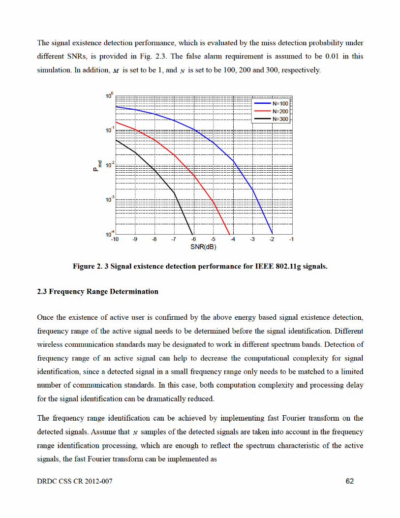
The signal existence detection perf01m ance, which is evaluated by the miss detection probability under

different SNRs, is provided in Fig. 2.3. The false alru.m requirement is assumed to be 0.01 in this

simulation. In addition, M is set to be 1, and N is set to be 100, 200 and 300, respectively .

.., E a..

-9 -8 -7 -6 -5

SNR(dB) -4 -3 -2 -1

Figure 2- 3 Signal existence detection performance for IEEE 802.11g signals_

2_3 Frequency Range Determination

Once the existence of active user is confi1med by the above energy based signal existence detection,

frequency range of the active signal needs to be dete1mined before the signal identification. Different

wireless communication standards may be designated to work in different spectrum bands. Detection of

frequency range of an active signal can help to decrease the computational complexity for signal

identification, since a detected signal in a small frequency range only needs to be matched to a limited

number of commlmication standards. In this case, both computation complexity and processing delay

for the signal identification can be dramatically reduced.

The fi:equency range identification can be achieved by implementing fast Fomier tr·ansfOim on the

detected signals. Assume that N sru.nples of the detected signals are taken into account in the frequency

range identification processing, which are enough to reflect the spectrum characteristic of the active

signals, the fast Fomier transf01m can be implemented as

DRDC CSS CR 2012-007 62

N-1 jZHkn

F(k)=L:y(n)e N k =O,l,···,N-1. (11) n=O

In the watchdog system, the interested spectrum range is classified into several smaller frequency

bands. The active signals will be sorted into one of these bands based on the obtained spectmm

characteristics.

The spectrum analysis for IEEE 802.11g signals is intr·oduced here to demonstrate the frequency range

identification. As described in the standard, IEEE 802.11g signals should work in the 2.4 GHz band

with a bandwidth of 22 MHz [75]. After detecting the existence of the signal, FFT is perf01med on the

received signal samples. The sampling frequency used in this simulation is 5.76 GHz, and the

obsetvation dmation is 4 us . The frequency range identification result is shown in Fig.2. 4. As shown in

the figme, there is an amplitude peak at the 2.4 GHz band. If we zoom in the peak range, we can see

that the 3d.B bandwidth of the detected signal is about 20 MHz. Based on this result, the detected signal

can be sorted into the 2.4 GHz frequency band.

00 0~~--4----+--~

i ::J

~-51-+---+-----t-E <(

1800 2000 2200 2400 2600 2800 3000 3200 Frequency{MHz)

Figure 2. 4 The spectrum analysis of the received IEEE 802.11g signals.

2.4 Feature Match based Signal Identification

The interested spectr11m range in this project (from 700 MHz to 6 GHz) is divided into 7 frequency

DRDC CSS CR 2012-007 63

DRDC CSS CR 2012-007 64

bands to assist the processing of the watchdog signal identification system, referring to the wireless

communication standards used in Canada [76]. The communication standards, such as GSM,

CDMA2000 and IEEE 802.11, are all taken into consideration. The classification of the interested

spectrum bands is presented in Table 1.

746~956MHz 1.66~2.0GHZ 2.1GHZ 2.3GHZ 2.4GHz 2.5GHz 5~6GHz GSM

(850MHz) GSM

(1.9GHz) W-CDMA (2.1GHz)

WiMAX (2.3GHz)

802.11b 802.11g 802.11n

WiMAX (2.3GHz)

802.11a (5GHz); 802.11n (5GHz)

IS-95 (800MHz)

IS-95 (1.9GHz)

Bluetooth

CDMA2000 (800MHz)

CDMA2000 (1.9GHz)

Zigbee

W-CDMA (850MHz)

W-CDMA (1.9GHz)

Table 2.1 The classification of spectrum bands in the watchdog system.

Feature match is developed for the signal identification in the watchdog system. The unique

characteristic of each standard is extracted and utilized to differentiate the identity of the signals.

Therefore, a local reference for each standard is generated based on the unique characteristic and saved

in the look-up table (Identification Table) for each frequency band. In the watchdog system, a sliding

correlator correlates the received signal against the local references, and triggers when a threshold is

exceeded.

In case that the active signals do not follow any wireless communication standards in Table 2.1, a blind

parameter estimation will be performed in the next section. In the following sections, we discuss the

signal identification processing for each frequency band. Finally, the performance of the proposed

signal identification techniques is evaluated by using the identification error probability.

2.4.1 746 MHz ~ 956 MHz Frequency Band

As shown in Table 1, GSM(850MHz), IS-95(800MHz), CDMA2000 (800MHz) and W-CDMA

(850MHz) coexist in the 746 ~ 956 MHz frequency band. Therefore, in order to differentiate one

standard from the other, we have to use their unique characteristics to differentiate them from each

other, following a signal is classified into this frequency range.

DRDC CSS CR 2012-007 65

2.4.1.1 GSM (850MHz)

The GSM standard is based on Time Division Multiple Access (TDMA) with eight fundamental

physical channels per carrier, each separated by 200 KHz. Therefore, one physical channel can be

defined as a sequence of TDMA frames [4]. According to [77], one TDMA frame consists of 8 time

slots with an interval of 15/26 ms and the data are transmitted in the form of bursts that are designed to

fit within these slots. Five different types of bursts exist in the system: normal burst, frequency

correction burst, synchronization burst (SB), access burst and higher symbol rate burst. The

synchronization burst carries details of the GSM frame structure and allows an MS to fully synchronize

with the base station (BS). In the watchdog system, we use the SBs for the downlink (DL) GSM signal

identification due to their fixed and periodic nature in downlink frame. As shown in Fig.2. 5, each SB

contains a training sequence that is extended to 64 bits. This extended sequence provides a larger

autocorrelation peak than the 26-bit sequence of the normal burst. It also allows larger multipath delay

spread to be resolved. The training sequence in each synchronization burst, which is used as the local

reference in the watchdog system, is designed as

{

}

_ 1,0,1,1,1,0,0,1,0,1,1,0,0,0,1,0,0,0,0,0,0,1,0,0,0,0,0,0,1,1,1,1,0,0,1,0,1,1,0,1,0,1,0,0,0,1,0,1,0,1,1,1,0,1,1,0,0,0,0,1,1,0,1,1

gsm dL =

(12)

Figure 2. 5 Synchronization burst structures in GSM.

According to [77], the normal format of training sequences is shown in Fig.2.6 after the differential

encoding process. These sequences have symmetrical patterns that can be easily detected using a

correlation function. Detection is accomplished by sliding the received signal sample and correlating it

with the local GSM reference sequence, then finding the correlation peak if any for signal feature

matching, as shown in Fig.2. 7.

DRDC CSS CR 2012-007 66

Figure 2.6 Training sequences in SB for normal format.

Figure 2.7 Block diagram of synchronization signal detection.

Suppose ( )y n is the received signal samples. The signal identification within the duration 64gsmN = can

be expressed by,

1

*_ _

0

1 ( ) ( )gsmN

gsm d gsm dngsm

I y n L nN

−

=

= ∑ (13)

The output of the above reference correlation function is always fed to a peak detector. A threshold is

involved to determine the peak which can be defined as the signal mean value. In order to further

confirm the existence of the GSM signals, we perform a peak period detection. In GSM, the interval

between synchronization signals is 10*8*15/26 = 46.15 ms. Thus, in 1 second there should be 21 peaks

for GSM and we put a timer in the proposed design to calculate the number of peaks in one time

period. The simulation is shown below:

~-----.-----.----.-----.----.-----.----.-----.----.----~

50

45

40

"" 35

~ 0::30 c: ,g ..!!! 25 ~ 820

15

10

Figure 2.8 Signal Identification Results for GSM.

For uplink (UL) GSM signal, similar to downlink signal identification processing, we utilize the 41-bit

u·aining sequence from Access Burst (AB) as local reference, which is given by

{ 0, 1, 0, 0, 1, 0, 1, 1, 0, 1,

1, 1, 1, 1, 1, 1, 1, 0, 0, 1,

1, 0, 0, 1, 0, 1, 0, 1, 0, 1,

0, 0, 0, 1, 1, 1, 1, 0, 0, 0}

(14)

Here, the interval between access bursts is the same as synchronization bursts in the downlink, i.e.

46.15 ms. Therefore, after local reference conelation, we could have 21 peaks within 1 second which

indicates the existence of GSM uplink signaL

2.4.1.2 IS-95 /CDMA2000 (800MHz)

The IS-95 air interface standard, after the first revision in 1995, was tetmed IS-95A, which specifies

the air interface for cellular with an 800MHz frequency band. The following CDMA2000 standard is

proposed by standardization committee TIA TR45.5 with the pmpose of providing data rates that meet

the IMT-2000 perf01mance requirements of at least 144 Kb/s in a vehicular environment, 384 Kb/s in a

pedesu·ian environment, and 2048 Kb/s in an indoor office environment CDMA2000 employs a multi

catTier scheme for the u·ansmission by using three consecutive IS-95B caniers where each catTier has a

chip rate of 1.2288 Mc/s. Hence, an identical identification scheme can be utilized for both standru·ds

while the bandwidth difference is used to distinguish between each other. The simple comparison DRDC CSS CR 2012-007 67

DRDC CSS CR 2012-007 68

between IS-95 and CDMA2000 is listed in Table 2.2.

Parameters IS-95 CDMA2000

Channel Bandwidth 1250kHz 5, 10, 15, 20 MHz

Number of duplex channels 832 2496

Table 2.2 Parameters comparison between IS-95 and CDMA2000.

In the watchdog system, we select the paging channel based correlation method to perform the signal

identification because the paging channel is used by both standards and possesses a fixed sequence

value for a certain period. The frame structure of paging channel is exhibited in Fig.2.9.

Figure 2.9 The paging channel frame structure.

The paging channel performs a number of different functions in addition to carrying paging messages

between the network and mobile users. It conveys general system information (e.g. the handover

thresholds), access information (e.g. the maximum allowed number of unsuccessful access attempts), a

list of the surrounding cells and channel assignment messages. Moreover, the paging channel executes

the wake up alert for both BS and MS during the communication. For instance, when one MS is in the

DRDC CSS CR 2012-007 69

‘idle’ mode, it constantly monitors one of the forward paging channels so that it can be alerted to the

presence of an incoming call at any time. Similarly when a MS sends out information, it will transmit

the paging ahead to inform the BS of the incoming signal. The paging channel is sub-divided into 80

ms slots and these are formed into maximum length cycles of 2048 slots, which correspond to a cycle

period of 163.84 s. The use of slots on the paging channel allows the system to support a ‘slotted

paging’ mode of operation, whereby a MS is only required to monitor the paging channel within

specific slots. This allows an MS to conserve power during periods where it is not required to monitor

the paging channel, thereby prolonging battery life. The frame structure of the paging channel is

exhibited in Fig. 2.10.

Figure 2.10 The paging channel message format.

The eight-bit MSG LENGTH field defines the length of the paging channel message in octets,

including the MSG LENGTH field itself, the message body and the checksum. The maximum value of

MSG LENGTH is 148, which allows a maximum message size of 1184 bits. The message body

contains the paging channel message information and the last 30 bits of the message are used to carry a

cyclic redundancy checksum (CRC) which is generated for the MSG LENGTH and message body

fields. The CRC generator polynomial for the paging channel is the same as that used for the sync

channel and is given by the equation below

30 29 21 20 15 13 12 11 8 7 6 2( ) 1g x x x x x x x x x x x x x x= + + + + + + + + + + + + + . (15)

The binary CRC sequence is as follows {1,1,0,0,0,0,0,0,0,1,1,0,0,0,0,1,0,1,1,1,0,0,1,1,1,0,0,0,1,1,1}.

Since the CRC exists at the end of each frame and maintains the same value, it can be utilized for the

signal identification for both IS-95 and CDMA2000. Consequently, the local reference stored in the

look-up table is the same as the CRC sequence, and after the sliding window correlation, there should

be peaks at the end of each frame which is an indicator for the existence of signals following IS-95 or

CDMA2000. To be specific, if the received signal is ( )y n , the correlation /I CI can be performed as

/ 1

*/ /

0/

1 ( ) ( )I CN

I C I CnI C

I y n L nN

−

=

= ∑ , (16)

DRDC CSS CR 2012-007 70

where / 32I CN = .

2.4.1.3 W-CDMA (850MHz)

Since no common signal frame structure exists for both the uplink (UL) and the downlink (DL) of the

W-CDMA standard, different scenarios have been proposed for detection.

W-CDMA system downlink physical channels are arranged into 10 ms radio frames which consist of

15 slots of 0.67 ms each. Each slot corresponds to 2560 chips or a chip rate 3.84 Mcps. The

synchronization channel (SCH) is one of the common downlink physical channels. The SCH consists

of two sub channels, the Primary and Secondary SCH. The 10 ms radio frames of the Primary and

Secondary SCH are divided into 15 slots. Fig.2.11 illustrates the structure of the SCH radio frame.

Figure 2.11 WCDMA synchronization channel (SCH) structure.

The Primary SCH consists of a modulated code of length 256 chips, namely, Primary Synchronization

Code (PSC), which is transmitted once every slot as shown in Figure 2. 11. Based on standard [78], the

PSC is generated through the following steps:

Define:

- a = <x1, x2, x3,…, x16> = <1, 1, 1, 1, 1, 1, -1, -1, 1, -1, 1, -1, 1, -1, -1, 1>

The PSC is generated by repeating a constant sequence modulated by a Golay complementary

sequence, and creating a complex-valued sequence with identical real and imaginary components. The

PSC( Cpsc) is defined as:

- Cpsc = (1 + j) * <a, a, a, -a, -a, a, -a, -a, a, a, a, -a, a, -a, a, a>;

where the leftmost chip in the sequence corresponds to the chip transmitted first in time. The

generation of PSC is shown in Figure 2. 12. Since PSC is constructed by repeating a constant sequence

(see Fig. 2.12) and is fixed to all cells, it can be detected using correlation functions.

DRDC CSS CR 2012-007 71

For W-CDMA signal recognition, we propose a matched filter due to better performance compared

with autocorrelation. The matched filter can be described as,

1

0

1 ( ) * ( )WN

W WnW

I y n L nN

−

=

= ∑ (16)

Figure 2.12 PSC sequence in WCDMA.

where ( )WL n is the PSC pattern at the k-th tap, and 256WN = denotes WCDMA’s synchronization

signal chip length for PSC. The matched filter structure is shown in Fig.2.13, where multipliers are

implemented using a multiplexer and a two’s complement converter, Fig. 2.14.

Figure 2.13 Match filter structure for WCDMA detection.

Figure 2.14 Multiplier implementation for match filter.

DRDC CSS CR 2012-007 72

Since the WCDMA signal is detected by a matched filter, a correlation peak is sufficient to recognize

WCDMA service without peak period calculation. However, a method might be required to recognize

the number of WCDMA cells in one area due to reuse of the same frequency band. The WCDMA’s P-

SCH period is 10/15 ms, which is 15 peaks in 10 ms. For instance, if 45 peaks are detected in 10 ms, it

means 3 cells exist around us.

For WCDMA uplink signals detection, there are two uplink dedicated physical and two common

physical channels:

• The uplink dedicated physical data channel (uplink DPDCH) and the uplink dedicated physical

control channel (uplink DPCCH);

• The physical random access channel (PRACH) and physical common packet channel (PCPCH).

The uplink DPDCH is used to carry dedicated data generated and there may be zero, one, or several

uplink DPDCHs together. The uplink DPCCH is used to carry control information. Control information

consists of known pilot bits to support channel estimation for coherent detection, transmit power-

control (TPC) commands, feedback information (FBI), and an optional transport-format combination

indicator (TFCI). The transport-format combination indicator informs the receiver about the

instantaneous parameters of the different transport channels multiplexed on the uplink DPDCH, and

corresponds to the data transmitted in the same frame. For each uplink signal there is only one uplink

DPCCH.

Figure 2. 15 Frame structure for uplink DPDCH/DPCCH

Based on the above, the feature being introduced is the same pilot sequence for each slot in one frame.

Different from the downlink signal detection, we perform the power autocorrelation to get the detection

peaks. Since there are 14 slots in one frame whose time length is 10 ms, after the power

DRDC CSS CR 2012-007 73

autocorrelation, 14 peaks would be detected for every 10 ms, determining the existence of W-CDMA

standard signal.

2.4.2 1.66 GHZ ~ 2.0 GHz Frequency Band

The communication standards working in the previous frequency band (746 MHz ~ 956 MHz) also

work in this spectrum range. The above signal identification techniques for GSM, IS-95, CDMA2000

and W-CDMA can also be employed in this frequency band. Therefore, we did not repeat the signal

identification techniques in this section. Please refer to the last section for the technique details.

2.4.3 2.1 GHz Frequency Band

In this frequency band, only W-CDMA signal exists. If a signal is active in this range, it can only be a

W-CDMA signal or some other irregular signals that require further blind parameter estimates.

Therefore, only the signal identification operation for W-CDMA is implemented in this frequency

band. For technique details, please refer to subsection 2.4.1.3.


This frequency band is allocated to WiMAX (IEEE 802.16) alone. The signal identification operation

in this frequency range is only to decide whether the active signal is WiMAX signal or not. In Canada,

WiMAX signals in this frequency are allocated two 15 MHz bands: 2305-2320 MHz and 2345-2360

MHz, and is intended for fixed and mobile services. It has been regionally licensed in Canada through

an auction process to a large number of licensees [82].

2.4.4.1 WiMAX (IEEE 802.16)

The WirelessMAN-OFDM physical layer (PHY) in IEEE 802.16 is based OFDM modulation and

designed for NLOS operation. The OFDM symbol, which has three types of subcarriers (i.e. data

subcarriers, pilot subcarriers and null subcarriers), can be mathematically expressed as:

DRDC CSS CR 2012-007 74

/22 ( )2

/20

( ) Reused

gc

used

Nj k f t Tj f t

kk Nk

S t e c e ππ ∆ −

=−≠

= ⋅

∑ (18)

where kc is the signal to be transmitted on the subcarrier whose frequency offset index is k , usedN is the

number of used subcarriers.

A preamble, which is structured as either one or two OFDM symbols, is inserted in the front of each

IEEE 802.16 signal frame. Each of those OFDM symbols contains a cyclic prefix (CP), which has the

same length as the cyclic prefix for data OFDM symbols. In downlink, the preamble is structured as

two OFDM symbols while it is structured as one OFDM symbol in the uplink.

The preamble in the downlink PHY protocol data unit consists of two consecutive OFDM symbols.

The first OFDM symbol uses only subcarriers whose indices are a multiple of 4. As a result, the time

domain waveform of the first symbol consists of four repetitions of 64-sample fragment, preceded by a

CP. The second OFDM symbol utilizes only even subcarriers, resulting in time domain structure

composed of two repetitions of a 128-sample fragment, preceded by a CP. This combination of the two

OFDM symbols is referred to as the long preamble in the IEEE 802.16 standard [83]. The time domain

structure of the DL preamble is illustrated in Fig. 2.16.

Figure 2.16 DL preamble structure in IEEE 802.16.

In the UL, the data preamble consists of one OFDM symbol utilizing only even subcarriers. The time

domain waveform consists of 2 128× samples preceded by a CP. This preamble is referred to as the

short preamble, as shown in Fig. 2.17.

Figure 2.17 UL preamble structure in IEEE 802.16.

DRDC CSS CR 2012-007 75

The frequency domain sequences for all full-bandwidth preambles are derived from the sequence in the

following equation:

( 100,100)ALLP − =

{ 1 ,1 , 1 ,1 ,1 ,1 , 1 ,1 ,1 ,1 ,1 , 1 ,1 ,1 , 1 ,1 , 1 , 1 ,1 ,1 ,1 ,1 , 1 ,1 ,1 ,1 , 1 ,1 ,1 ,1 ,1 , 1 ,1 ,1 , 1 ,1 , 1 , 1 ,

1 , 1 ,1 ,1 , 1 ,1 ,1 ,1 ,

j j j j j j j j j j j j j j j j j j jj j j j j j j j j j j j j j j j j j j

j j j j j j j j

− − − − + − − − + − − − + − − + + − − + − − − − −− + − − − − + − − − + − − − + − − + + − − + − − − −− − + − − − − + − − −1 ,1 ,1 ,1 ,1 , 1 ,1 ,1 , 1 ,1 , 1 ,j j j j j j j j j j j+ − − − + − − + + − − + − −

1 ,1 , 1 ,1 ,1 ,1 , 1 ,1 ,1 , 1 ,1 ,1 ,1 , 1 ,1 , 1 , 1 ,1 , 1 ,1 ,1 ,1 , 1 , 1 , 1 , 1 ,1 , 1 , 1 ,1 , 1 , 1 , 1 ,1 , 1 ,1 ,1 ,

1 ,1 , 1 , 1 , 1 ,1 ,0, 1

j j j j j j j j j j j j j j j j j j jj j j j j j j j j j j j j j j j j j

j j j j j j j

− − − − + + + − − + + + − − + + + − + − − + − + − − +− − + − − − − − − − + − − − − − + − − − − − − − − + − −− + − − + − + − − + − − ,1 , 1 , 1 , 1 ,1 ,1 ,1 , 1 ,1 ,1 ,1 ,j j j j j j j j j j j+ − + − + − − + + + − − + − −

1 , 1 , 1 , 1 , 1 ,1 , 1 , 1 , 1 ,1 ,1 ,1 , 1 ,1 ,1 ,1 , 1 ,1 ,1 , 1 , 1 ,1 ,1 ,1 ,1 , 1 , 1 , 1 ,1 , 1 ,1 ,1 ,1 , 1 , 1 , 1 ,

1 , 1 , 1 , 1 , 1 ,1 ,1 ,1 ,1

j j j j j j j j j j j j j j j j j jj j j j j j j j j j j j j j j j j j

j j j j j j j j

− − + − + − + − + − − − − − − + − + + − + − − − − + −− − − − − − + + + + − − − + − + + − − − − + − − − − − −+ − − − + − + − + − − −

}

, 1 ,1 ,1 , 1 ,1 , 1 , 1 , 1 ,1 ,1 ,1 , 1 ,1 ,1 ,1 ,1 , 1 , 1 , 1 , 1 ,1 , 1 , 1 ,1 , 1 , 1 , 1 ,1 , 1 , 1 , 1 ,1 , 1 ,1 ,1 ,1 , 1 , 1 , 1 , 1 ,1 ,1 ,1

j j j j j j j j j jj j j j j j j j j j j j j j j j j jj j j j j j j j j j j j j j j j

− − + + + − − + − + − + − − ++ + − − + − − − − + − + − + − + − − − − − − − + − − − −− − + − + − + − − + + + + − − − − − − − − + − −

(19)

DRDC CSS CR 2012-007 76

The frequency domain sequence for the 4 64× sequence 4 64P × is defined by

mod 4

4 64( )mod 4

2 2 ( ( )) 00 0

ALLk

conj P k kPk×

⋅ ⋅ == ≠

. (20)

The frequency domain sequence for the 2 128× sequence EVENP is defined by

mod 2

( )mod 2

2 ( ) 00 0ALL

EVEN kP k kP

k ⋅ ==

≠. (21)

The time domain representations of both long preamble and short preamble in IEEE 802.16 can be

easily derived by substituting (20) and (21) into (18). As shown in the above analysis, both long

preamble and short preamble in IEEE 802.16 are generated from fixed sequences which are specially

designed for the IEEE 802.16 system. These preambles provide unique characteristics for the signal

identification.

One more issue needs to be taken into account for the IEEE 802.16 signal identification is the length of

cyclic prefix in the preambles. In the standard, the length of cyclic prefix in the preambles is required to

be the same as the CP of data OFDM symbols, which is not a fixed value. However, since the length of

cyclic prefix in IEEE 802.16 can only be 1/4, 1/8, 1/16 or 1/32 of the symbol length, we can just test

these four scenarios. Therefore, both long preamble and short preamble, with 4 different lengths of CP

are saved in the Identification Table for the signal identification of IEEE 802.16.

Let 16UL and 16D

L denote the local reference for uplink and downlink IEEE 802.16 signals, respectively.

The correlation based signal identification can be written as

16 /

/

/

*802.16 16

116

1 ( ) ( )U D

U D

U D

N

nI y n L n

N =

= ∑ , (22)

where 16UN = [264 272 288 384] and 16D

N = [528 544 576 768].

DRDC CSS CR 2012-007 77


The 2.4 GHz spectrum range is allocated to Wi-Fi (IEEE 802.11, IEEE 802.11b, IEEE 802.11g and

IEEE 802.11n), Bluetooth and ZigBee for communications in Canada. However, since the 2.4 GHz

band is one of the industrial, scientific and medical (ISM) radio bands, other devices, such as

microwave ovens, baby monitors and cordless telephones, also operate in this band. In the signal

identification process of the proposed watchdog system, we only attempt to match the received signal

with the three communication standards (i.e. Wi-Fi, Bluetooth and Zigbee). All the signals following

other formats are taken as irregular signals and further processed using blind parameter estimation

processing. The signal identification techniques for these three communication standards are presented

as follows.

2.4.5.1 Wi-Fi (IEEE 802.11)

IEEE 802.11 is a set of standards for implementing wireless local area network (WLAN). The most

popular WLAN protocols in the 2.4 GHZ band include 802.11b, 802.11g and 802.11n, which define a

series of over-the-air modulation techniques. Therefore, the watchdog system has to identify signals

that follow these three specifications separately.

IEEE 802.11b

IEEE 802.11b is a DSSS based transmission scheme in the 2.4 GHz band. In IEEE 802.11b, a physical

layer convergence procedure (PLCP) preamble is inserted in the beginning of each signal frame, which

includes a PLCP synchronization (SYNC) field and a PLCP start frame delimiter (SFD). The SYNC

field consists of 128 bits of scrambled ones and the SFD is a 16-bit field: [1111 0011 1010 0000] (MSB

to LSB, and LSB is transmitted first in time). The 144 bits PLCP preamble will last for 144 us in each

signal frame [84]. In the IEEE 802.11b standard, this 144 bits PLCP preamble is referred to as long

PLCP preamble, as shown in Fig. 2.18.

DRDC CSS CR 2012-007 78

Figure 2.18 Long PLCP format in IEEE 802.11b.

In addition, a short PLCP preamble and header is also defined in IEEE802.11b for an optimal mode

that allows data throughput at the higher rates. This is another signal format for IEEE 802.11b signals,

which should also be taken in to account in the signal identification processing. The short PLCP format

is presented in Fig. 2.19.

Figure 2.19 Short PLCP format in IEEE 802.11b.

The short SYNC filed consists of 56 bits of scrambled “0” bits, where the initial state of the scrambler

is [001 1011]. The short SFD is the bit pattern [0000 0101 1100 1111]. And the period of the short

PLCP preamble is only 72us [84].

The periodic PLCP preamble provides a unique characteristic for the IEEE802.11b signal, and can be

extracted for signal identification. The local references for the IEEE802.11b signal identification

( 11 _b LL and 11 _b SL ), which are stored in the Identification Table, are just the long and short PLCP

preambles after the 1 Mbit/s DBPSK modulation. In order to achieve the feature detection, the received

signal will be re-sampled using the sampling frequency indicated in the IEEE802.11b standard. The

DRDC CSS CR 2012-007 79

signal identification for IEEE 802.11b can be achieved by:

11 _ 1

*802.11 _ 11 _

011 _

1 ( ) ( ),b LN

b L b Lnb L

I y n L nN

−

=

= ∑ (23)

and

11 _ 1

*802.11 _ 11 _

011 _

1 ( ) ( ),b SN

b S b Snb S

I y n L nN

−

=

= ∑ (24)

where 11 _ 144b LN = and 11 _ 72b SN = .

IEEE 802.11g

IEEE 802.11g is an OFDM based transmission scheme in the 2.4GHz band. Each physical frame of

IEEE 802.11g starts with two training sequences (also called PLCP preamble), as shown in Fig. 2.20.

Figure 2. 20 PLCP preamble in IEEE 802.11g.

As shown in the Figure 2., 1t to 10t denote the short training symbols and 1T and 2T denote two long

training symbols. The total training length is 16 us. A short OFDM training symbol consists of 12

subcarriers, each of which is modulated by the elements of the sequence S , which is given by

{

}

26,26 13 / 6 0,0,1 ,0,0,0, 1 ,0,0,0,1 ,0,0,0, 1 ,0,0,0,1 ,0,0,0,1 ,0,0,0,0,0,0,0, 1 ,0,0,0, 1 ,

0,0,0,1 ,0,0,0,1 ,0,0,0,1 ,0,0,0,1 ,0,0

S j j j jj j j j

j j j j

− = × + − − + − −− − + − − − −

+ + + + (25)

DRDC CSS CR 2012-007 80

The multiplication factor 13/ 6 is used to normalize the average power of the resulting OFDM

symbol, which utilizes 12 out of 52 subcarriers [75]. The short training signal is generated according to

the following equation:

/ 2( 2 )

/ 2( ) ( )

ST

ST

Nj k Ft

short Tshort kk N

r t w t S e π ∆

=−

= ∑ (26)

where ( )Tshortw t is the time-windowing function depending on the short training sequence duration,

STN denotes the number of total subcarriers, and F∆ is the subcarrier spacing.

A long OFDM training symbol consists of 53 subcarriers (including a zero value at dc), which are

modulated by the elements of the sequence L , given by

{

}

26,26 1,1, 1, 1,1,1, 1,1, 1,1,1,1,1,1,1, 1, 1,1,1,1,1, 1,1,1,1,1,0,1, 1, 1,1,1, 1,1, 1,1, 1,1, 1, 1, 1,1,1, 1, 1,1, 1,1, 1,1,1,1,1

L− = − − − − − −− − − − − − −− − − − − − − −

(27)

The long OFDM training symbol is generated according to the following equation:

12

/ 2( 2 ( ))

/ 2( ) ( )

STG

ST

Nj k F t T

long Tlong kk N

r t w t L e π ∆ −

=−

= ∑ , (28)

where ( )Tlongw t is the time-windowing function depending on the long training sequence duration, and

12 1.6GT us= . Two periods of the long sequence are transmitted for improved channel estimation

accuracy, yielding 1.6 2 3.2 8Tlong us= + × = . The corresponding time domain expression of the short

training sequence and long training sequence in IEEE 802.11g can be found in Appendix.

Since the training sequences are fixed and highly periodic, the detection of these training sequences can

be used to indicate the existence of the signals following the IEEE 802.11g standard. The time domain

expression of both short training sequence and long training sequence is used as the local reference,

and is stored in the Identification Table of the watchdog system.

In order to confirm whether the received signal is IEEE802.11g signal, the received signal will be re-

DRDC CSS CR 2012-007 81

sampled using the sampling frequency 250 KHz that described in the IEEE802.11g standard. Let 11gL

denote the local reference for the 802.11g signal identification. The signal identification processing,

which is to correlate the received signal ( )y n with 11gL , can be formulated as

11

*802.11 11

111

1 ( ) ( )gN

g gng

I y n L nN =

= ∑ , (29)

where 11 320.gN = If the detected signal is IEEE 802.11g signal, a correlation peak can be observed.

Otherwise, due to the low correlation between the local reference 11gL and the signals following other

standards, we cannot see a significant correlation peak.

Our simulation result for the IEEE 802.11g signal identification when IEEE 802.11g signals are active

is presented in Fig. 2.21. In this simulation, IEEE 802.11g signals are transmitted by the active users.

The communication environment is assumed to be AWGN channel with a SNR of 10 dB. As shown in

the figure, periodic correlation peaks can be observed due to the periodicity of the training sequence.

In order to demonstrate that the correlation peaks can only be observed when IEEE 802.11g signals are

active, the scenario with only IEEE 802.11b active signals is tested in the simulation. The correlation

result between IEEE 802.11b signals and the local reference 11gL in the identical communication

environment is presented in Fig.2.22. No significant correlation peaks can be observed. Fig. 2.23

provides the simulation result for the coexistence of IEEE 802.11b and IEEE 802.11g signals in AWGN

channel. Due to the weak correlation between IEEE 802.11b signals and the local reference 11gL , as well

as the strong correlation between IEEE 802.11g signals and 11gL , reliable signal identification can still

be achieved with a SNR of 10 dB.

Considering that the practical communication environment may be more complex and hostile, a non-

line-of-sight (NLoS) multipath channel with a SNR of 0 dB is also adopted to demonstrate the

proposed IEEE 802.11g signal identification scheme. The simulations are carried out for the scenarios

that only 802.11g signal exists, only 802.11b signal exists and both 802.11g and 802.11b signals

coexist. The results are shown in Fig. 2.24 – Fig. 2.26. In this hostile communication environment, we

can still get a significant correlation peak though the peak value is attenuated.

0.8 -:::J 1/) Q)

a:: 0.6 c:: 0

~ Q) t::

0.4

0 {)

0.2

0

-0.2 2000 4000 6000 8000 10000 12000 14000

Sample Index

Figure 2. 21 Signal Identification for IEEE 802.11g signals when only 802.11g signals exist

(AWGN channel with a SNR of 10 dB).

0.8 :; 1/) Q)

0::: 0.6 c:: 0

:;::. ro Q) t::

0.4

0 ()

0.2

0

-0.2 2000 4000 6000 8000 10000 12000 14000

Sample Index

Figure 2. 22 Signal Identification for IEEE 802.11g signals when only 802.11b signals exist


DRDC CSS CR 2012-007 82

0.8 -:::J 1/) Q) 0:: 0.6 c:: 0

16 0.4

~ 0 ()

0.2

0

-0.2 2000 4000 6000 8000 10000 12000 14000

Sample Index

Figure 2- 23 Signal Identification fo1· IEEE 802.11g signals when 802.11b and 802.11g signals coexist


0.8 -:::J 1/) (I)

0.6 0:: c:: 0

~ 0.4 ~

'-0 ()

2000 4000 6000 8000 10000 12000 14000 Sample Index

Figure 2- 24 Signal Identification for IEEE 802.11g signals when only 802.11g signals exist

(Multipath channel with a SNR of 0 dB).

DRDC CSS CR 2012-007 83

0.8 -"3 (/) Q)

0:::: 0.6 c: 0 :;

0.4 (j) t:: 0 l)

0.2

2000 4000 6000 8000 10000 12000 14000 Sample Index

Figure 2. 25 Signal Identification for IEEE 802.11g signals when only 802.11b signals exist


0.8 -"S (/) Q)

0:::: 0.6 c: 0

:;:::. m

0.4 (j) '-'-0 ()

2000 4000 6000 8000 10000 12000 14000

Sample Index

Figure 2. 26 Signal Identification fot· IEEE 802.11g signals when 802.11b and 802.11g signals coexist

DRDC CSS CR 2012-007 84

DRDC CSS CR 2012-007 85


IEEE 802.11n

IEEE 802.11n is developed based on previous 802.11 standards by adding multiple-input multiple-

output (MIMO) and 40 MHz channels to the PHY, and frame aggregation to the MAC layer. The High-

Throughput (HT) PLCP preamble of IEEE 802.11n signal can also be adopted for the signal

identification due to its unique format. In IEEE802.11n standard, two formats are defined for the

PLCP: HT-mixed format and HT-greenfield format. For the HT-mixed format operation, the preamble

has a non-HT portion and an HT portion. The non-HT portion of the HT-mixed format preamble

enables detection of the PPDU and acquisition of carrier frequency and timing by both HT stations

(STAs) and STAs that are compliant with IEEE 802.11b/g [85]. The HT portion of the HT-mixed

format preamble enables the MIMO channel estimation to support demodulation of the HT data by HT

STAs, which is particularly designed for IEEE 802.11n. For HT-greenfield operation, a particular HT-

greenfield format preamble is introduced. Therefore, the HT-portion of the HT-mixed format preamble

and the HT-greenfield format preamble can be utilized for the signal identification.

Two local references for IEEE 802.11n signal identification are derived from the HT-portion of the

HT-mixed format preamble and the HT-greenfield format preamble, respectively. For the HT-mixed

format preamble, the fixed HT short training field (HT-STF) with a duration of 4 us, which is used to

improve automatic gain control estimation in a MIMO system, can be extracted as the local reference.

The frequency sequence used to construct the HT-STF in a 20 MHz transmission is presented in (30).

In a 40 MHz transmission, the HT-STF is constructed from the 20 MHz version by duplicating and

frequency shifting and by rotating the upper subcarriers by 90° [85].

For 20MHz transmission:

{

}

28,28 1/ 2 0,0,0,0,1 ,0,0,0, 1 ,0,0,0,1 ,0,0,0, 1 ,0,0,0,1 ,0,0,0,1 ,0,0,0,0,0,0,0, 1 ,0,0,0, 1 ,0,0,

0,1 ,0,0,0,1 ,0,0,0,1 ,0,0,0,1 ,0,0,0,0

HTS j j j jj j j jj j j j

− = × + − − + − −− − + − − − −

+ + + + (30)

For 40MHz transmission:

DRDC CSS CR 2012-007 86

{58,58 1/ 2 0,0,1 ,0,0,0, 1 ,0,0,0,1 ,0,0,0, 1 ,0,0,0, 1 ,0,0,0,1 ,0,0,0,0,0,0,0, 1 ,0,0,0, 1 ,0,0,0,1 ,0,0,0,1 ,0,0,0,1 ,0,0,0,1 ,0,0,0,0,0,0,0,0,0,0,0,0,0,0,0,1 ,0,0,0, 1 ,0,0,0,1 ,

HTS j j j j jj j j j j

j j j jj

− = × + − − + − − − −+ − − − − + ++ + + − −

+

}0,0,0, 1 ,0,0,0, 1 ,0,0,0,1 ,0,0,0,0,0,0,0, 1 ,

0,0,0, 1 ,0,0,0,1 ,0,0,0,1 ,0,0,0,1 ,0,0,0,1 ,0,0j j j j

j j j j j− − − − + − −

− − + + + +

(31)

The time domain representation of the transmission in transmit chain is as follows [12]

1( ) ( )

HT STFHT STF TToneSTS HT STF

r t w tN N −−

−

=⋅

(32)

[ ] ( )1

exp 2 ( )SR STS

STS

SR STS

N Ni

k k k F CSk N i

Q HTS j k t Tπ=− =

ϒ ∆ −∑ ∑

For the values of the related parameters in (32), please refer to the IEEE standard 802.11n [85].

For the HT-greenfield format, the High-Throughput Greenfield Short Training field (HT-GF-STF) is

placed at the beginning of an HT-greenfield format frame. The time domain waveform for the HT-GF-

STF on transmit chain can be expressed as [85]:

1( ) ( )

HT GF STFHT GF STF TToneSTS HT GF STF

r t w tN N − −− −

− −

=⋅

(33)

[ ][ ] ( )1

exp 2 ( )SR STS

STS

SR STS

N Ni

k HTLTF k k F CSk N i

Q P S j k t Tπ=− =

ϒ ∆ −∑ ∑

where

1 1 1 11 1 1 11 1 1 11 1 1 1

HTLTFP

− − = − −

(34)

The waveform defined by (33) has a period of 0.8 μs, and the HT-GF-STF includes ten such periods,

with a total duration of = 8 μs.

Let 11 mnL and 11 gnL denote the local references saved in the look-up table, which are the time domain

representation of the HT-STF in HT-mixed format preamble and HT-GF-STF in the HT-greenfield

DRDC CSS CR 2012-007 87

format preamble, respectively. The signal identification operation for IEEE 802.11n can be

mathematically described as

11 (11 ) 1

*802 11 11 (11 )

011 (11 )

1 ( ) ( )n nm g

m g

m g

N

n n nnn n

I y n L nN

−

=

= ∑ . (35)

2.4.5.2 Bluetooth (IEEE 802.15.1)

The Bluetooth devices operate in the unlicensed 2.4 GHz ISM band. Bluetooth, ratified as IEEE

Standard 802.15.1, uses a radio technology called frequency-hopping spread spectrum, which chops up

the data being sent and transmits chunks of it on up to 79 bands (1 MHz each; centered from 2402 to

2480 MHz) in the range 2,400-2,483.5 MHz (allowing for guard bands). In addition, Bluetooth is

designed for low power consumption with a short communication range. The maximum transmission

power is limited to 20 dBm [86].

In Bluetooth, every packet starts with an access code, which is used for synchronization, DC offset

compensation, and identification. If a packet header follows, the access code is 72 bits long; otherwise,

the access code is 68 bits long and is known as a shortened access code. The access code identifies all

packets exchanged on a physical channel: all packets sent in the same physical channel are preceded by

the same access code. The access code format is shown in Fig. 2.27.

Figure 2.27 The access code format in Bluetooth.

The preamble is a fixed zero-one pattern of four symbols used to facilitate dc compensation. The

sequence is either 1010 or 0101, depending on whether the LSB of the following sync word is 1 or 0.

The sync word is a 64-bit code word derived from a 24-bit address (lower address part (LAP)).

Therefore, the sync word will depend upon the type of access code, one of:

• CAC (Channel Access Code): used when connected, generated from the LAP of the master

device.

• DAC (Device Access Code): used for paging, generated from the LAP of the paged device.

DRDC CSS CR 2012-007 88

• IAC (Inquiry Access Code): used for inquiring. For general inquiries, the GIAC (General IAC)

is used, generated from the reserved LAP of 9E8B33.

Since both master’s LAP and slave’s LAP are generally unknown for the proposed watchdog system,

the sync word cannot be used for signal identification. As a result, the local reference for Bluetooth

signal identification will only be the first part of the transmitted access code, which is derived from

15.1_1 [10101]S = and 15.1_ 2 [01010]S = . (36)

Let 15.1_1L and 15.1_ 2L denote the local references for Bluetooth, the correlation based signal identification

process can be formulated as

4*

802.11 15.1_1/20

1 ( ) ( )5n

nI y n L n

=

= ∑ (37)

The local references 15.1_1L and 15.1_ 2L are short and may not be reliable enough for the signal

identification. Therefore, the 1 MHz bandwidth requirement and the 20 dBm power restriction are

combined to identify the Bluetooth signals in the proposed watchdog system. The bandwidth and the

power of the detected signal will be first evaluated. If and only if these two parameters meet

requirements of the Bluetooth standard, the correlation between the detected signal and the local

reference is operated for further confirmation. Once one of these three factors is denied, the detected

signal will be taken as a irregular signal and processed using blind parameter estimation.

2.4.5.3 Zigbee (IEEE 802.15.4)

Zigbee, based on the IEEE standard 802.15.4, intends to offer the fundamental lower network layers of

a type of wireless personal area network (WPAN) which focuses on low-cost, low-speed ubiquitous

communication between devices. Similar to the other wireless communication standards, the

synchronization header of each data unit in IEEE 802.15.4 can be extracted for signal identification.

The format of the PHY protocol data unit of IEEE 802.15.4 is shown in Fig. 2.28.

DRDC CSS CR 2012-007 89

Figure 2. 28 The format of the PHY protocol data unit of IEEE 802.15.4.

In the synchronization header (SHR), the preamble field is used by the transceiver to obtain chip and

symbol synchronization with an incoming message, which is of 32 binary zeros. The start-of-frame

delimiter (SFD) is an 8 bit field indicating the end of the synchronization (preamble) field and the start

of the packet data. The sequence of the SFD is 11100101 [87].

Since this synchronization header is inserted in the beginning of each data unit, it provides a unique and

periodic characteristic for the IEEE 802.15.4 signals. Therefore, the local reference 15 4L saved in the

Identification Table for ZigBee signal identification is the transmitted SHR after a 16-ary quasi-

orthogonal modulation, which has a duration of 160 us. Then, the correlation based signal identification

can be expressed as

15 4

*802.15.4 15.4

115.4

1 ( ) ( )N

nI y n L n

N =

= ∑ , (38)

where 15 4 40.N =

2.4.6 2.5 GHZ Frequency Band

WiMAX (IEEE standard 802.16) works in this frequency band. Since the physical signal format in this

frequency band is the same as that in the 2.3 GHz, the signal identification technique presented in

Section 4.4.1 can be employed. For the technique details, please refer to Section 4.4.1.

2.4.7 5 GHz ~ 6 GHz Frequency Band

IEEE 802.11a and IEEE 802.11n signals coexist in this frequency band.

DRDC CSS CR 2012-007 90

2.4.7.1 IEEE 802.11a

IEEE 802.11a uses the same OFDM based transmission scheme as 802.11g [75]. The difference is that

IEEE 802.11a operates in the 5 GHz band while IEEE 802.11g works in the 2.4 GHz band. Therefore,

the IEEE 802.11a signal can also be identified by using the training sequences presented in Appendix I.

For the look-up table generation and the signal identification techniques, please refer to subsection

4.5.1.2.

2.4.7.2 IEEE 802.11n

The IEEE 802.11n signal in this frequency band share the same format as that of the IEEE 802.11n

signal working in 2.4 GHz. Therefore, the same signal identification technique introduced in subsection

4.5.1.3 can be adopted.

2.4.8 Signal Identification Performance Evaluation

If there are M communication standards coexist in a frequency band, 1M + hypotheses have to be

considered for the signal identification, that is

0 0 0

1 1 1

: ( ) ( ) ( ): ( ) ( ) ( )

: ( ) ( ) ( )M M M

y n x n w ny n x n w n

y n x n w n

= + = + = +

HH

H (39)

where 0 ( )x n denotes the scenario of non-standard compliant signal, ( ), 1, ,mx n m M= denotes the

signal following m -th standard. Let the binary variable ma indicate the existence of the signal in the

hypothesis mH , where 1 represents the presence of signal ( )mx n and 0 represents the absence of this

signal. The received signal in the watchdog system can be written as

0

( ) ( ) ( )M

m mm

y n a x n w n=

= +∑ . (40)

For the identification of signal following communication standard i , the correlation result ir can be

DRDC CSS CR 2012-007 91

expressed as

1*

0

1 1* *

0 0 0

1 ( ) ( )

1 1( ) ( ) ( ) ( )

i

i i

N

i iniN NM

m m i in m ni i

r y n L nN

a x n L n w n L nN N

−

=

− −

= = =

=

= +

∑

∑∑ ∑ (41)

where ( )iL n denotes the local reference for standard i , iN is the length of the local reference. If 0ia = ,

(41) can be rewritten as

1 1

* *,0

0, 0 0

1 1( ) ( ) ( ) ( )i iN NM

i m m i im m i n ni i

r a x n L n w n L nN N

− −

= ≠ = =

= +

∑ ∑ ∑ . (42)

With the central limit theorem, 1

*

0

1 ( ) ( )iN

m ini

x n L nN

−

=∑ can be approximated as a zero-mean Gaussian

distributed variable with a variance of 2,m iσ . Therefore, the first term of (42) is Gaussian distributed with

a mean of zero and a variance of 2 2,

0,

M

m m im m i

a σ= ≠∑ . Similarly, the correlation between noise and the local

reference can be approximated as a zero-mean Gaussian variable with a variance of 21 *

2

0

( )iNi

wn i

L nN

σ−

=

∑ .

Therefore, the complete correlation result when 0ia = can be modeled as

21 *2 2 2

,0 ,0, 0

( )~ 0,iNM

ii m m i w

m m i n i

L nr N aN

σ σ−

= ≠ =

+

∑ ∑ . (43)

For the situation that 1ia = , (41) can be rewritten as

1 1 1* * *

,00 0, 0 0

1 1 1( ) ( ) ( ) ( ) ( ) ( )i i iN N NM

i i i m m i in m m i n ni i i

r x n L n a x n L n w n L nN N N

− − −

= = ≠ = =

= + +

∑ ∑ ∑ ∑ , (44)

where ( ) ( )i ix n L n= . Therefore, the first term of (44) will be a constant that equals to 1

2

0

1 | ( ) |iN

ini

L nN

−

=∑ . The

analysis of the second and third terms in (44) is the same as that for the situation 0ia = . The entire

con-elation result when a; = 1 can be modeled as

Cl> a..-

... ......

' 2 ~

\

3\

\

\

~

' ' ' "' ' ' \ ~

\

\

\ -5 0 5

SNR(dB)

-e- A.1 1g 0.3

......._ A.1 1g = 0.5

---+- A.1 1g = 0.8

"'I. ........... -,..., ~

10 15

Figure 2. 29 Error probability of IEEE 802.11g signal identification when IEEE 802.11b and

IEEE 802.11g signals coexist.

Let A, denote the threshold selected to identify the signals following standard i , where 0 < A.; < 1, the

identification en or probability ~. can be expressed as

DRDC CSS CR 2012-007 92

+.F;,l 1- Q

(46)

where f;,0 and f;,1 are the probabilities that the signals followin standard i are resent and absent

respectively, and ~.o + ~.1 = 1 . QO denotes the Q-func on.

For the scenario that both IEEE 802.11b and IEEE 802.11g signals coexist in the 2.4 GHz band without

inegular signals, the identification en or probability for the IEEE 802.11 g signal identification can be

rewritten as

~lg

(47)

+ .F;,l 1-Q

where N11g = 320 , 2 a b,g ~ 0.003 1 andN~t[~tg(n) l

2

= 0.0031 . Under the n=O Nllg

DRDC CSS CR 2012-007 93

DRDC CSS CR 2012-007 94

assumption that the presence and absence of IEEE 802.11g signals are equally probable in the test area,

the identification error probability will be

11 11

2 2

11 11

2 2

11 1 12 20.0031(1 ) 0.0031(1 )

112 0.0031(1 ) 0.0031(1 )

g gI e

w w

g g

w w

P Q Q

Q Q

λ λ

σ σ

λ λ

σ σ

− = + −

+ + − = +

+ +

(48)

The identification error probability for the IEEE 802.11g signal identification in the SNR range

between -10 dB and 15 dB is plotted in Fig. 2.29. In this simulation, the threshold is set to be 0.3, 0.5

and 0.8 respectively.

As shown in the figure, a very low identification error probability can be obtained by the proposed

watchdog system at low SNRs, especially when a proper identification threshold is selected. If the

threshold is set to be 0.5, the identification error probability will be as low as 410− when the SNR is -7

dB.

2.5 Conclusion

We address the multi-stage signal existence detection and identification techniques for the proposed

watchdog sensor network in this section. The existence of an active signal is determined by signal

energy detection using a pre-determined background noise level related threshold. The frequency range

of active signals is then determined using the FFT based spectrum analysis, in order to limit the number

of potential communication standards used for feature-matching based signal identification. Moreover,

the category of the detected signal, i.e. which communication standard it follows, is identified by using

the inherent time/frequency domain characteristics of each communication standard. The signal

existence detection, frequency range determination and signal identification, as well as the related look-

up table generation and identification error probability are theoretically analyzed. Simulation results are

also presented to validate the proposed signal existence detection and identification techniques for the

proposed watchdog sensor network.

DRDC CSS CR 2012-007 95

Section 3 Blind Parameter Estimation and Automatic Modulation Classification in Watchdog Sensor Network

3.1. Introduction

Various blind OFDM system parameters estimation schemes have been studied in recent years for both

signal identification and signal behaviour analysis. The existing techniques can be generalized into two

categories: with or without sampling frequency at the transmitter as prior information. The first

category has been widely explored in [88]-[90], most of which ([88]-[89]) focused on the

synchronization parameters or on one or two other parameters ([90], [91]). [92] and [93] presented a

more complete OFDM system parameters extraction which employed the correlation method to explore

the system parameters of OFDM systems. However, this kind of techniques cannot apply to the

considered public security problem due to the unknown information of incoming signals especially for

intrusion signal.

For signal detection purpose, blind parameter estimation without any prior information is investigated.

Among those system parameters, the decisive one is the sampling frequency at the transmitter and there

are two primary approaches under current research: cyclostationarity-based and correlation-based

estimation. Cyclostationary theory, developed for years in various signal processing areas, was first

introduced into OFDM system analysis in [88] and based on Dandawate and Giannakis' work, the key

step to estimate sampling frequency through cyclostationary method is to define the cyclo-period.

Martin and Kedem [95] detected the period via the periodogram associated with the sequence having

the similar period to the least common multiple periods of the original cyclostationary signal. Hurd and

Gerr [96] obtained the cyclo-period from the bispectrum, which was estimated using the two-

dimensional periodogram. Dandawate and Giannakis [94] aimed at the detection of cyclo-stationarity

under a broader context, almost cyclostationary signals, through a statistical test based on the cyclic

covariance and the cyclic spectrum. [97] presents the cyclostationarity-based sampling frequency

estimation through Dandawate and Giannakis’ approach. On the other hand, a non-parametric method

for blind parameter estimation which is based on spectrum information and autocorrelation is an

alternative. [98] provides the complete investigation. Unfortunately, the method does not work well for

raised cosine upsampling at the transmitter which is closer to the practical implementation. In the first

part of this section, we propose sequential steps to estimate the key parameters for OFDM systems

under blind scenario based on cyclostationary analysis and spectrum information.

DRDC CSS CR 2012-007 96

Automatic modulation classification (AMC) is used to automatically identify the modulation scheme

used in an intercepted communication signal by analyzing the characteristics of the received signal,

which is normally corrupted by the noise and fading channels. The interest in blind modulation

classification has been growing since the late eighties [99]. Such technique plays several important

roles in both civilian and military applications including signal surveillance, data interception, signal

identification, interference monitoring, and counter-measure development. Legitimate signals in

defence communications should be securely transmitted and received, whereas hostile signals from

adversaries must be identified and recovered through modulation classification. The transmitting

frequencies of these signals of interest may range from high frequency bands to ultra high frequency

bands and their signal format can vary from traditional simple narrowband modulations to newly

introduced wideband schemes particularly, OFDM. Under such diverse conditions, advanced

modulation classification techniques are needed for real-time signal interception and processing, which

are vital for decisions involving electronic warfare operations and other tactical actions [99].

As no prior knowledge of the incoming signal is available under military circumstances, the design of a

modulation classifier essentially involves two steps: preprocessing of the incoming signal for the

elimination of the impact of irrelevant system parameters (frequency and timing offset, channel, etc.)

and proper identification of modulated signals. Estimation of additional system parameters other than

the modulation scheme has been discussed in the first part. Automatic classification of modulation

schemes, which is the main subject of second part of this section, includes two general categories,

namely, decision-theoretic and pattern recognition based methods.

In general, the decision-theoretic approach is based on some likelihood function or approximation

theory [100]-[104], where the modulation classification can be deemed as a multiple-hypothesis test, or

can be further converted into a sequence of pair-wise hypothesis tests. Once the appropriate likelihood

functions are established, average likelihood ratio test (ALRT) [100], generalized likelihood ratio test

(GLRT) [101], or hybrid ALRT/GLRT (HLRT) [103] can be adopted as potential solutions. The

decision-theoretic classifiers with maximum likelihood (ML) are optimal, but the corresponding close-

form solutions are unavailable due to the high complexity of the model used. In addition, this approach

is not robust with respect to the model mismatch in the presence of phase or frequency offsets, residual

channel effects, and so on.

On the other hand, in the pattern recognition approach [104]-[110], the modulation classification

module is composed of two subsystems, i.e., a feature extraction subsystem, which extracts the key

features from the received signal; and a pattern recognizer, which processes those features and

DRDC CSS CR 2012-007 97

determines the modulation scheme of the intercepted signal according to a pre-designed decision rule.

The most commonly used features are higher-order statistics (HOS), including cumulants and

moments. A hierarchical framework based on fourth-order cumulants is proposed in [104]. A

combination of second and fourth-order cyclic cumulants’ (CC) magnitudes is investigated in [105]

while higher-order up to eighth-order CC is adopted in [106] and nth-order warped CC magnitudes is

utilized in [107]. Statistical moments of the signal phase are used in [108]. Cumulants are preferred due

to their favourable properties over moments [111].

In contrast to the decision-theoretic methods, the pattern recognition methods may be non-optimal but

simple to implement and can often achieve near-optimal performance if carefully designed.

Furthermore, the pattern recognition methods are more robust with respect to the aforementioned

model mismatches in the decision-theoretic approach. Therefore, we focus on the pattern recognition

modulation classification approach and two new pattern recognition based approaches are proposed in

time-domain and frequency-domain, respectively.

As for the proposed time-domain approach, a Gaussian Mixture Model (GMM)-based classifier is

designed to recognize various modulation schemes from the received signal. The Gaussian mixture

model has been successfully used in the past for speech identification and verification. The basis of this

approach is to represent the distribution of training signals from each modulation with a weighted sum

of several multivariate Gaussian functions. The parameters used in the model can be estimated using

the iterative Expectation-Maximization (EM) algorithm.

However, due to impact of multipath fading channels, severe AMC classification accuracy degradation

can be introduced due to the channel model mismatch. Therefore, HOS is introduced based on the

frequency domain feature for OFDM signals since the channel impact for each subcarrier is reduced to

a gain factor in frequency domain. HOS is a mathematical tool for the determination of high order

statistical characteristic of a random process, which not only can remove the influence of Gaussian

noise, but also eliminate the rotation of the constellation diagram.

In the last part of the section, the lab testing platform is introduced to verify the various proposed

algorithms for blind parameter estimation and modulation classification. The lab testing platform for

the algorithm verification contains an R&S® SMJ100A vector signal generator for signal generation, a

R&S® FSP spectrum analyzer for signal observation, and a PXI 5105 high speed digitizer for signal

data collection and storage. Our proposed algorithms for blind OFDM system parameter estimations

and modulation classification are evaluated using the signals generated from Rohde&Schwarz (R&S®)

DRDC CSS CR 2012-007 98

and re-captured by the National Instruments (NI) signal acquisition system. In our evaluation process,

an IEEE 802.11a baseband signal is generated by R&S® SMJ100A vector signal generator, sampled and

saved by the NI PXI 5105 high speed digitizer. The signal captured by the NI PXI 5105 is then used to

verify the proposed algorithms in MATLAB.

3.2 Parameter Estimation of Unknown OFDM Signal

3.2.1 Carrier Frequency Estimation

To estimate the carrier frequencies , with the number of signals components

present in an observed spectrum, one can use a nonparametric approach based on a Fast Fourier

Transform (FFT) [112]. This method is appropriate for narrowband signals above the noise floor

provided that the frequency resolution is high enough. One can assume that the observed compound

signal has been sampled at least twice the maximum bandwidth of interest : , with the

received sample data stream

and its Power Spectral Density (PSD) ( is the number of samples). Note that the larger the number

of samples, the higher the frequency resolution provided by the FFT grid. This is a crucial parameter to

detect signals having a small bandwidth. However, if the FFT size is too large, the sequence of length

can be divided into blocks of size , then one can perform FFTs of length and add the

contribution of each block given by . The carrier frequencies are then estimated by detecting the

band-edges and for all with a threshold between the noise level and the

signal level. The carrier frequencies are then estimated as

3.2.2 Sampling Frequency Estimation

After down conversion, the next step of the blind estimation process is to extract the sampling

frequency or the oversampling factor . We introduce the existing cyclic spectrum analysis method

proposed by Dandawate and Giannakis [7]. If the signal is cyclostationary with cyclic-frequency for

DRDC CSS CR 2012-007 99

delay , the estimator gives by

where is given by

is the estimate of , the cyclic-autocorrelation at cyclic frequency which is given

by

and is the asymptotic covariance matrix of the estimator , which can be computed by the

equation in [94].

Fig .3.1. Simulation Results of Oversampling Estimation

Subsequently, the oversampling factor can be given by , where is the estimated cyclic

frequency in radian. Mean Square Error (MSE) of oversampling estimation method is shown in Fig. 3.1

under different channel scenarios.

3.2.3 Number of Subcarriers Estimation

To realize this step we exploit autocorrelation properties of the received sequence. The autocorrelation

of the received sequence which corresponds to the second-order/one-conjugate cyclic cumulants at zero

cyclic frequency in the work of [98] can be written as

l'il-:1!

1"' r (fd = N L x(i)~" (f ·- k)~ i=o

(6)

with k the shift index. One can assume that the autoconelation function is cyclically shifted; that is,

two vectors x are concatenated in order to cope with the data outside the interval .f E [Q, •.. N - 1].

Therefore, a central peak in the autocon elation function can be obse1ved in Fig. 3.2 .

Based on the above, the first half of autoconelation length is equal to that of received oversampled

signal. With peak detection, we can get the index inte1val between center peak and the peak in first half

easily, denoted as l\\1i: . Using the estimated oversampling factor !f from last section, Ns is given by

/il = .t!i;j, ~ q ,

~~--~----~--~~--~----~--~----~----~

250

200

150

100

50

Autooorrelation Index of Received Signal

Fig.3.2. Autocorrelation of Received Oversampled Signal

DRDC CSS CR 2012-007 100

DRDC CSS CR 2012-007 101

Fig.3.3. Estimation Error for Number of Subcarriers

3.2.4 Joint estimation of CP length, frequency and timing offset

The joint estimation of CP length and the timing/frequency offset is presented in this sub-section. Since

the OFDM signal itself is a cyclostationary signal at a delay , when was estimated from the

above step, we can employ (3) with for estimating the corresponding cyclo-frequency or

symbol duration , and find .

Also from [88] and [89], the frequency and timing offset can be obtained by using the cyclostationary

statistics. After downsampling, we assume the signal at this step is raised cosine pulse shaping under

multipath Rayleigh channels. Considering the timing offset and the frequency offset , the signal

can be given by

Due to the introduction of the CP, when the delay , the correlation term can be rewritten as

where is the set of which are inside CP and

DRDC CSS CR 2012-007 102

can be approximated due to the central limit theorem as Gaussian noise. When the number of

OFDM symbols for the estimation is large, the frequency offset ε can be given by

where is the estimate of cyclic-correlation at cycle frequency 0 and delay . After obtaining

the frequency offset as in (18), we use eqn.(21) of [88] to obtain the timing offset , i.e.

where is estimated earlier.

3.3 Decision-Theoretic-based Automatic Modulation Classification

The decision-theoretic (DT) modulation classification approach provides an optimal solution in the

sense that it minimizes the probability of false classification if all assumptions of other system

parameters are met. Within the DT approach, AMC is formulated as a multiple composite hypothesis-

testing problem, and the corresponding hypothesis is resolved using maximum likelihood techniques.

Various methods for the determination of the maximum likelihood have been proposed for DT-AMC

based upon different assumptions regarding other unknown signal parameters. An in-depth

understanding of the validity of this assumption is critical to proper selection of an AMC technique for

a particular scenario.

Three different decision-theoretic algorithms have been developed in the literature: average likelihood

ratio test (ALRT), generalized likelihood ratio test (GLRT) and hybrid likelihood ratio test (HLRT).

ALRT is a popular AMC approach applied to phase shift keying (PSK) and quadrature amplitude

modulation (QAM). ALRT treats unknown system parameters in the received signal as random

variables (R.V.'s) and the likelihood functions (LF) are obtained by an averaging process. This requires

a hypothesis for the probability density functions (PDF) of the R.V.'s. If the actual PDF coincides with

the hypotheses, the modulation classification results are optimal. The LF under the hypothesis ,

representative of the th modulation, , where is the total number of candidate

modulation schemes, is given by

DRDC CSS CR 2012-007 103

where is the conditional LF of the noisy received signal under , conditioned on the

modulated value for the th modulation scheme , and is the priori PDF of under .

The pre-known PDF of enables us to reduce the problem to a simple hypothesis-testing problem by

integrating over . The ALRT is computationally intensive but current microprocessors have made the

ALRT feasible. In general, the performance of ALRT-AMC is very sensitive to estimation errors of

other system parameters such as symbol timing, baud rate, carrier frequency, carrier phase, pulse shape,

and noise power. The accuracy of ALRT is also affected by channel fading and the type of noise

present.

The GLRT treats the modulation scheme candidates as unknown deterministic values and the maximum

likelihood test is applied as if the true values were known. The best performance is achieved by the so-

called uniformly most powerful (UMP) test [113]. When a UMP test does not exist or is difficult to

derive, a logical procedure is introduced to estimate the unknown quantities. Assuming is true,

these estimates are then used in a likelihood ratio test, as if they were correct. If the maximum

likelihood (ML) is used for estimates, the test is called GLRT. It can be seen that GLRT treats the

unknown quantities (including both the parameters and data symbols) as deterministic unknowns, and

the LF under is given by

The HLRT is a hybrid approach that models the data symbols as discrete random variables uniformly

distributed over the modulation scheme alphabet set and treats the carrier phase as a deterministic

variable. This is a combination of the aforementioned two modulation classification approaches, for

which the LF under is given by

where and are vectors of unknown quantities modelled as unknown deterministic and

random variables (RV), respectively. Usually, and consist of parameters and data symbols,

respectively.

DRDC CSS CR 2012-007 104

3.3.1 ALRT-based Algorithms

With all other system parameters perfectly known, ALRT leads to a modulation classification algorithm

whose performance can be considered as a benchmark. The data symbols in the received

signal are treated as independent and identically distributed (i.i.d.) RVs. The LF under hypothesis is

computed by averaging over the constellation points corresponding to the th modulation format. To

begin with, consider the ALRT for classifying PSK/QAM modulation signals. For the th

hypothesis , the joint log-likelihood function can be expressed as

where

and is a symbol-based received complex data series of length , preprocessed from the

intercepted signal emitted from a non-cooperative transmitter through an AWGN channel with a two-

sided power spectral density of , and is a complex number and is the th

reference state of the th modulation type. The decision of modulation classification is achieved based

on the following criterion: choose , as the modulation scheme in the intercepted signal if

is a maximum.

Consider now the histogram test when the received signal is real [133]. This test is very popular in

AMC practice for classifying real variables, such as modulation phase, frequencies, or amplitudes. The

histogram is constructed from a density table [124] with the intervals shown on the x-axis and the

number of occurrences in each interval represented by the height of a rectangle located above the

interval. To determine the similarity between the ALRT and the histogram test, we choose both

and to be real values, where is the jth reference of the modulation

type. A table is constructed by dividing the histogram up into the intervals , and

counting the number of ’s occupying the interval, denoted by , for . If

is bounded by {- , i.e., for all , we find

DRDC CSS CR 2012-007 105

If

where

Therefore the quantized version of (1) will be

Notice that the data series is the histogram value of , for , with bins, and

is the template associated with . In the limit as , the results of the histogram test

approach the results of the ALRT, showing that the histogram test is a special case of the ALRT. It is

also remarkable that (4) – (8) provide asymptotic optimal templates for the histogram test.

3.3.2. GLRT- and HLRT-based Algorithms

As the ALRT algorithm suffers from high computational complexity in most realistic scenarios, GLRT

and HLRT algorithms have been investigated as possible solutions to identify linear modulations. In

AWGN and with, the LF for GLRT and HLRT are respectively given by [113]

where is a finite summation over all the possible constellation points of the th modulation, for

the th interval. T is the signal length for pulse shaping filter and S is the signal power. is the PSD

of zero-mean AWGN. is the carrier frequency offset. GLRT has some implementation advantages

over ALRT and HLRT, as it avoids the calculation of exponential functions and does not require the

knowledge of the noise power to compute the LF.

DRDC CSS CR 2012-007 106

3.4 Pattern Recognition-based Automatic Modulation Classification

The design of a feature based (FB) modulation classification algorithm first relies on some features

extracted from the intercepted signal followed by a decision-making process [122]. Sample features of

the received signal considered for modulation classification include the variance of the centred

normalized signal amplitude, phase and frequency [123], the variance of the zero-crossing interval

[124, 125], the variance of the magnitude of the signal wavelet transform (WT) after peak removal

[126-128], the phase PDF [129–131] and its statistical moments [132-134], moments, cumulants, and

cyclic cumulants of the signal itself [135-137] etc.

3.4.1 Instantaneous Amplitude Phase and Frequency-based Algorithms

The most intuitive way to identify the modulation scheme used in the incoming signal is to explore the

information embedded in its instantaneous amplitude, phase and frequency. To extract such

information, different methods have been developed in the literature. The following different features

in various modulated signals are often employed for modulation classification:

Frequency shift keying (FSK) signals are characterized by constant amplitude, whereas amplitude shift

keying (ASK) signals have varying amplitudes, and similarly, PSK signals contain information in the

varying phase. The maximum of the discrete Fourier transform (DFT) output of the centred (the term

‘centred’ specifies that the average is removed from the data set, i.e., DC-free signal) and normalized

instantaneous signal was used as a feature to distinguish between FSK and ASK/PSK modulated

signals.

ASK signals have no information in their absolute phases and BPSK signals possess only real valued

constellation points whereas M-PSK does possess phase information. Therefore, the variance of the

absolute centred and normalized phase can be used to distinguish between M-PSK and real-valued

constellations. The variance of the direct (not absolute) centred normalized phase is used to distinguish

between BPSK and ASK modulation schemes. A binary decision tree structure is employed to

differentiate modulation schemes between classes, and furthermore, within each class, as we will

briefly mention later. At each node of the tree, the decision is made by comparing a statistic against a

threshold.

In [131] and [132], the variance of the zero-crossing interval is used as a feature to distinguish FSK

from PSK and the unmodulated waveform (UW). The zero-crossing interval is a measure of the

DRDC CSS CR 2012-007 107

instantaneous frequency, and it is a staircase function for FSK signals, whereas for UW and PSK

signals it is a constant. The AMC is treated as a two hypothesis testing problem: for FSK and

for UW and PSK. The hypotheses are formulated based on the Gaussian assumption for the estimated

feature, that is , with the hypothesis-dependent mean and variance (the

mean is actually the theoretical value of the feature under whereas the variance is estimated under

each hypothesis). An LRT is used for the decision which, due to the Gaussian assumption, is simplified

to the comparison of the feature with a threshold h derived from the LRT. The average probability of

classification error is then given by

where is the complementary error function defined as

The variance of the instantaneous frequency is also employed in [133] [134] to discriminate FSK from

UW and PSK. The decision is made by comparing the feature against a threshold.

3.4.2 Wavelet Transform-based Algorithms

The use of the wavelet transform to localize the changes in the instantaneous frequency, amplitude and

phase of the received signal was also introduced to AMC. The distinct behaviour of the Haar WT

(HWT) magnitude for PSK, QAM and FSK signals was employed for modulation identification in [36–

38]. For a PSK signal, the HWT magnitude is a constant. On the other hand, because of the frequency

and amplitude variations in FSK and QAM, the HWT magnitude is a staircase function with peaks at

phase changes. These peaks do not provide useful information for non-continuous phase FSK signals.

PSK and FSK signals are of constant amplitude, where amplitude normalization has no effect on their

HWT magnitude. Therefore, the variance of the HWT magnitude with amplitude normalization was

used to discriminate FSK from PSK and QAM. Furthermore, the variance of the HWT magnitude

without amplitude normalization was employed to distinguish between QAM and PSK. The decisions

were made by comparing the features against some thresholds, based on the statistical analysis of the

features, to minimize the probability of classification error for PSK signals [135]–[137].

DRDC CSS CR 2012-007 108

3.4.3 Signal statistics-based Algorithms

To discriminate among BPSK, ASK, M-PSK and QAM, the cumulant-based feature was adopted,

where the nth-order/q-conjugate cumulant of the output of the matched filter is calculated at the zero

delay vectors. To make the AMC decision, an LRT based on the PDF of the sample estimate of the

feature was formulated to achieve minimum probability of classification error. The moment-based

feature was used in [136], where the nth-order/q-conjugate moment of the output of the matched filter

is calculated at the zero delay vectors. The goal is to distinguish between PSK and QAM modulation

schemes. A joint power estimation and classification was performed in [136]. The decision was made

based on the minimum absolute value of the difference between the sample estimate and prescribed

values of the feature. Reference [137] combined several normalized moments and cumulants for

training a neural network to identify FSK, PSK and QAM in multipath environments.

Cumulant-based features were proposed in [135] with details to identify the order of ASK, PSK, and

QAM modulations, which can be summarized as follows: the normalized cumulant of fourth-

order/two-conjugate for ASK is ; the magnitude of the normalized cumulant of fourth-

order/zero-conjugate for PSK is ; and the normalized cumulant of fourth-

order/zero-conjugate for QAM is . The theoretical values of the nth-order/q-conjugate

cumulant, , even, for several linear modulations are given in [99]. These values

were computed using the moment to cumulant formula in which the nth-order moments were calculated

as ensemble averages over the noise-free unit-variance constellations with equiprobable symbols. Note

that owing to the symmetry of the signal constellations considered, the nth-order moments for odd

are zero and hence, using the moment to cumulant formula, it is easy to show that the nth-order

cumulants for odd are also zero. A LRT was formulated based on the PDFs of the sample estimates

of features, which are Gaussian, that is, . With a simplified approximation of equal variances

under all the hypotheses, the decision was further reduced to comparing the sample estimate of the

chosen feature against a threshold, with as any of the cumulant-based features previously

mentioned. For an hypothesis testing problem, with the hypotheses ordered such

that , the decision rule is to choose if

DRDC CSS CR 2012-007 109

where and .

The above method was extended in [138] to classify linear modulations in frequency-selective

channels. The blind alphabet matched equalization algorithm, which is used for equalization, was also

employed for modulation classification. Some other cumulant-based features were added [129] to the

set of features extracted from the instantaneous amplitude, phase and frequency to include QAM

signals in the set of candidate modulations to be recognized.

Signal moments were applied to distinguish between QPSK and 16QAM. Specifically, a linear

combination of the fourth-order/two-conjugate moment and the squared second-order/one-conjugate

moment were employed, with the coefficients and the delay vector optimized to maximize the

probability of correct classification. The signal-moment feature was employed to identify the

order of QAM signals in [138], with the decision made based on the minimum absolute value of the

difference between the sample estimate and prescribed values of the feature.

Signal cyclostationarity was also exploited for linear modulation identification, via two approaches:

spectral line generation by passing the signal through different nonlinearities, and periodic fluctuations

with time of cumulants up to the nth-order. We note that the nth-order cyclic frequencies (CFs) are

given by , where m is an integer. The nth-order CF formula also holds for an IF signal,

where is replaced by the IF frequency, . With this property, the cyclostationarity of the received

signal was exploited for AMC through a pattern of sine-wave frequencies in signal polynomial

transformations. For example, the and sinusoids that appear in the second and fourth powers

of the received signal, respectively, were used in [138] to distinguish between BPSK and QPSK. In

[139] the same property was explored for a baseband modulated signal. By increasing the order of the

nonlinear signal transformation beyond fourth powers, this argument can be extended to identify

modulations of order higher than QPSK. Note that the quasi-optimal algorithm derived within the LB

framework for PSK signal classification also exploits such a property, by using the information

extracted in the time domain. However, the signal cyclostationarity is not exploited in this work, as the

sampling is performed at the symbol rate .

DRDC CSS CR 2012-007 110

3.5 Proposed Algorithms for AMC

Through the technology survey in the previous section, we found that the feature based modulation

classification algorithms provide a good trade-off between classification accuracy and computational

complexity. In this section we propose two approaches to realize automatic modulation classification

which are based on time-domain and frequency-domain feature analysis of the intercepted signals. The

GMM is used to analyze the time-domain features while HOS is used to perform modulation

classification from the frequency-domain features of the signal.

3.5.1 GMM-based Automatic Modulation Classification

In this section, the proposed GMM-based AMC is described in detail. A brief introduction to the GMM

with parameter extraction and training is given as well as an introduction to the Kolmogorov-Smirnov

(K-S) Test to classify the modulation type from the received signal.

3.5.1.1 Gaussian Mixture Model

A Gaussian Mixture Model (GMM) is a parametric probability density function represented as a

weighted sum of Gaussian component densities. GMMs are commonly used as a parametric model of

the probability distribution of continuous measurements or features in a biometric system such as,

vocal-tract related spectral features in a speech recognition system. GMM parameters are estimated

from training data using the iterative Expectation-Maximization (EM) algorithm or Maximum A

Posteriori (MAP) estimation from a well-trained prior model.

A GMM is a weighted sum of M component Gaussian densities given by the following equation,

where is a D-dimensional continuous-valued data vector (i.e., measurement or features),

, are the mixture weights, and are the component Gaussian

densities. Each component density is a D-variant Gaussian function of the form,

DRDC CSS CR 2012-007 111

with mean vector and covariance matrix . The mixture weights satisfy the constraint that

. The complete Gaussian mixture model is parameterized by the mean vectors, covariance

matrices and mixture weights from all component densities. These parameters are collectively

represented by the notation,

There are several variants of the GMM shown in (16). The covariance matrices, , can be full rank or

constrained to be diagonal. Additionally, parameters can be shared or tied among the Gaussian

components, e.g., having a common covariance matrix for all components. The choice of model

configuration (number of components, full or diagonal covariance matrices, and parameter tying) is

often determined by the amount of data available for estimating the GMM parameters and how the

GMM is used in a particular biometric application.

It is also important to note that because the Gaussian components are combined together to model the

overall feature density, full covariance matrices are not necessary even if the features are not

statistically independent. The linear combination of diagonal covariance basis Gaussians is capable of

modeling the correlations between feature vector elements. The effect of using a set of M full

covariance matrix Gaussians can be equally obtained by using a larger set of diagonal covariance

Gaussians.

GMMs are often used in biometric systems, most notably in speech recognition systems, due to their

capability of representing a large class of sample distributions. One of the powerful attributes of the

GMM is its ability to form smooth approximations to arbitrarily shaped densities. The classical uni-

modal Gaussian model represents feature distributions by a position (mean vector), an elliptic shape

(covariance matrix) and a vector quantizer (VQ) or nearest neighbor model. A GMM acts as a hybrid

between these two models by using a discrete set of Gaussian functions, each with their own mean and

covariance matrix, to allow for better modeling capability.

DRDC CSS CR 2012-007 112

Figure 3.4. Comparison of distribution modeling. (a) histogram of a single cepstral coefficient from a 25 second utterance by a male speaker (b) maximum likelihood uni-modal Gaussian model (c) GMM and its 10 underlying component densities (d) histogram of the data assigned to the VQ centroid locations of a 10 element codebook [140].

Figure 3.4 compares the densities obtained using a uni-modal Gaussian model, a GMM and a VQ

model. Plot (a) shows the histogram of a single feature from a speech recognition system (a single

cepstral value from a 25 second utterance by a male speaker); plot (b) shows a uni-modal Gaussian

model of this feature distribution; plot (c) shows a GMM and its ten underlying component densities;

and plot (d) shows a histogram of the data assigned to the VQ centroid locations of a 10 element

codebook. The GMM not only provides a smooth overall distribution fit, its components also clearly

detail the multi-modal nature of the density.

The use of a GMM for representing feature distributions in a biometric system may also be motivated

DRDC CSS CR 2012-007 113

by the intuitive notion that the individual component densities may model some underlying set of

hidden classes. For example, in speech recognition, it is reasonable to assume the acoustic space of

spectrally related features corresponding to a speaker’s broad phonetic events such as vowels, nasals or

fricatives. These acoustic classes reflect some general speech dependent vocal tract configurations that

are useful for characterizing speaker identity. The spectral shape of the ith acoustic class can in turn be

represented by the mean of the ith component density, and variations of the average spectral shape

can be represented by the covariance matrix . Because all the features used to train the GMM are

unlabeled, the acoustic classes are hidden in that the class of an observation is unknown. A GMM can

also be viewed as a single-state HMM with a Gaussian mixture observation density, or an ergodic

Gaussian observation HMM with fixed, equal transition probabilities. Assuming independent feature

vectors, the observation density of feature vectors drawn from these hidden acoustic classes is a

Gaussian mixture.

3.5.1.2 Maximum Likelihood Parameter Estimation

Given training vectors and a GMM configuration, we wish to estimate the parameters of the GMM

which in some sense best matches the distribution of the training feature vectors. There are several

techniques available for estimating the parameters of a GMM. By far the most popular and well-

established method is maximum likelihood (ML) estimation. The aim of ML estimation is to find the

model parameters which maximize the likelihood of the GMM given the training data. For a sequence

of T training vectors , the GMM likelihood, assuming independence between the

vectors, can be written as,

Unfortunately, this expression is a non-linear function of the parameters and direct maximization is not

possible. However, ML parameter estimates can be obtained iteratively using a special case of the

expectation-maximization (EM) algorithm.

The basic idea of the EM algorithm is, beginning with an initial model , to estimate a new model ,

such that . The new model then becomes the initial model for the next iteration and the

process is repeated until some convergence threshold is reached. The initial model is typically derived

DRDC CSS CR 2012-007 114

by using some form of binary vector quantizer (VQ) estimation. On each EM iteration, the following

re-estimation formulas are used which guarantee a monotonic increase in the model’s likelihood value,

Mixture Weights

Means

Variances (diagonal covariance)

The a posteriori probability for component is given by

Based on the procedures above, the database of Gaussian Mixture Model for different modulation

schemes can be established and the AMC is realized through the Kolmogorov-Smirnov test.

The received signal consists of information containing the signal component and noise:

where is assumed to be one of modulation schemes and is an additive white Gaussian noise

(AWGN) process of zero mean and covariance function and is assumed to be uncorrelated with

. is the data length of the received signal. The task here is to employ GMM into each modulation

scheme to obtain the primary parameters (weights, mean values and variances).

Modulation Types

QPSK 0.45 0.55 0.22 0.62 1.23 1.54

16QAM 0.31 0.69 2.34 7.15 2.22 2.56

64QAM 0.22 0.78 12.12 20.54 3.45 3.99

DRDC CSS CR 2012-007 115

256QAM 0.15 0.85 34.23 50.78 4.02 4.11

Table 3.1: Parameter estimations for different modulation schemes based on GMM

3.5.1.3 Kolmogorov-Smirnov (K-S) Test

The Kolmogorov-Smirnov (K-S) test is a non-parametric test of goodness of fit for the continuous

cumulative distribution of the data samples. It can be used to approve [120] the null hypothesis that two

data populations are drawn from the same distribution to a certain required level of significance. On the

other hand, failing to approve the null hypothesis shows that they are from different distributions. With

the GMM database established above, we can obtain the approximated PDFs for different modulation

schemes. Therefore, the K-S test is performed on the received signal with the interference from a

fading channel and noise. The K-S test is used to determine the distance from either the PDF above or

the modulation type.

We consider K-S test in this section. In this test, we are given a sequence of i.i.d. real-valued data

samples , with the underlying cumulative distribution function (CDF) , and a

hypothesized distribution with the CDF , The null hypothesis to be tested is

The K-S test first forms the empirical CDF from the data samples

where is the indicator function, which is equal to one if the input is true, and zero otherwise. The

largest absolute difference between the two CDF’s is used as the goodness-of-fit statistic, given by

and in practice is calculated by

The significance level of the observed value is given by

with

DRDC CSS CR 2012-007 116

The hypothesis is rejected at a significance level 𝛼 if .

3.5.2 HOS-based Modulation Classification

Before introducing the proposed algorithm, definitions, properties and computations of the HOS (i.e.,

moments and cumulants) of a stationary random process are discussed. The emphasis of the discussion

is mainly on fourth order statistics and orders higher than four will not be considered.

3.5.2.1 Moments

For a collection of random variables , let denote the set of

component indices of . The joint moment of x is given by

According to (30), the th moment of a set containing k random variables is the expectation of the

product of these k random variables. It then follows that

and the second, third and fourth moments are

The foregoing equations are the basic moment equations which will be used for the derivation of

fourth-order cumulants in the following subsection.

3.5.2.2 Cumulants

For a collection of random variables and the set of component indices

of , if we have , then is the subvector consisting of those components of x

whose indices belong to I. The "partition" of set I is the unordered collection of nonintersecting

DRDC CSS CR 2012-007 117

nonempty sets such that = I.

Denote the moment and cumulant of the subvector as and , the moment-to-cumulant

(M-C) formula is

where denotes summation over all partitions of the set I and Q is the number

of the subsets of a partition.

According to the M-C formula (34), the first cumulant is equal to the first moment, that is

The second cumulant is

The third cumulant, , is

The fourth cumulant, , is

The second, third and fourth cumulants are usually called variance, skewness and kurtosis. In statistics

and probability theory, kurtosis is a statistical measure of the "peakedness" of the probability

distribution of a random variable. It measures the flatness of a distribution density function near its

center. Positive values are used to indicate that a density is more peaked around its center than a normal

curve and negative values indicate that a density is more spread out around its center than a normal

curve.

As for a Gaussian process, i.e., AWGN, all cumulants of order greater than two are identically zero.

Non Gaussian processes do not have all zero cumulants. Thus, higher-order cumulant measurements

have a natural tolerance to Gaussian noise.

DRDC CSS CR 2012-007 118

3.5.2.3 Proposed Modulation Classification Algorithm for OFDM Systems

Since the shape of the amplitude distribution of different modulation schemes is characterized by

kurtosis, it provides a statistical metric for modulation scheme classification. By calculating the higher-

order cumulants of independent symbols over each subcarrier in OFDM systems, the corresponding

modulation scheme can be classified according to the computed value and the theoretical value.

The nth-order/q-conjugate moment of the frequency domain symbol over the kth subcarrier can

be calculated as

where is the frequency domain symbol transmitted within the lth symbol period and the kth

subcarrier and L is the number of total samples taken into consideration.

By using the M-C formula (34), the nth-order/q-conjugate cumulant of the constellation can be

easily expressed in terms of moments as

The theoretical values of the nth-order/q-conjugate cumulants, , for the constellations of interest

are given in Table 3.2. These values were computed using the M-C formula in which the nth-order/q-

conjugate moments calculated as ensemble averages over the noise-free constellations with

equiprobable symbols under the constraint of unit energy. Due to the symmetry of the considered

constellation, the nth-order/q-conjugate moments are equal to zero when n is odd. Therefore, only the

nth-order/q-conjugate cumulants when n is even are given. These theoretical values will be used as the

catalogue patterns for decision making of the classifications in the next subsection.

BPSK QPSK 16QAM 64QAM

1 0 0 0

1 1 1 1

-2 1 -0.68 -0.619

-2 0 0 0

-2 -1 -0.68 -0.619

DRDC CSS CR 2012-007 119

Table 3.2: Theoretical cumulants for constellations under constraint of unit variance

3.5.3 Performance Analysis of Data Recovery

In this section, we will consider the effects of synchronization error on modulation classification and

data recovery. Note the subsequent analysis is for an OFDM signal. The synchronization errors include

sampling clock frequency offset (SFO) and carrier frequency offset (CFO). At the receiver, we assume

that the carrier frequency is , and the sampling rate is . Therefore the carrier frequency

offset, , and the relative sampling rate offset, , are designated as

After sampling at the sampling rate and removing the guard interval, the th received symbol can

be represented by N samples

If we assume the channel is an AWGN channel, the N received samples of the OFDM signal with the

effects of CFO and SCO can be represented as,

As already mentioned, during the acquisition process, the CFO and timing offset have been estimated

and pre-compensated for in the time domain (before modulation classification). The ICI produced by

the remaining CFO is smaller when compared to Gaussian noise, which can be considered as a

complex zero mean Gaussian noise. In (43), is an attenuation factor close to 1. Considering the

effects of a frequency selective fading channel and neglecting the factor , (43) is modified as

As (44) indicates, a phase rotation occurs when the subcarrier sample is transmitted. The rotated phase

is given by,

DRDC CSS CR 2012-007 120

where is the phase of the fading channel .

The rotated phase can be calculated as follows:

If the channel is a slowly fading channel the difference of rotated phases between two adjacent symbols

can be represented as:

The introduced joint tracking algorithm uses D-symbol delay linear least squares, as shown in Figure

3.5 (c). When the remaining CFO and SCO are relatively small or the noise is very large, the difference

in the rotated phases between two adjacent symbols is very small, as shown in Figure 3.5 (a). This may

result in poor estimation accuracy and in some cases may even give estimation results of the opposite

sign. If we compare the phase rotation of the current symbol with the next D symbol that delays D-

symbol-interval, the effects of noise may be reduced to some extent, as shown in Figure 3.5 (c). In this

case, (46) is modified as

Applying the same least squares estimation technique to (48), the improved method is presented as

(49). When D is equal to , the RMS (root-mean-square) of the estimation error can be minimized.

DRDC CSS CR 2012-007 121

Figure 3.5. The principle of D-symbol estimation.

3.6 Lab Testing Platform and Results

The proposed lab testing platform for the algorithm verification contains a R&S® SMJ100A vector

signal generator (shown in Fig. 3.6) for IEEE 802.11a signal generation, a R&S® FSP (shown in Fig.

3.7) spectrum analyzer for signal observation, and a PXI 5105 high speed digitizer (Fig. 3.8) for signal

data collection and storage. The setups for the testing are introduced in the following section and the

platform can be seen in Fig. 3.9.

3.6.1 Hardware and Software Specifications

The evaluations described in this part are based on the following hardware and software specifications

as shown in Table 3.3 and Table 3.4, respectively.

3.6.2 Equipment Interconnections and Setup

A R&S® SMJ100A vector signal generator is used to generate IEEE 802.11a signals to test the

proposed modulation classification in OFDM signals. SMJ100A covers all data rates that are supported

by the WLAN standards IEEE 802.11a, IEEE 802.11b and IEEE 802.11g with complete channel

coding. Among these standards, the IEEE 802.11a is employed for algorithm evaluation.

Figure 3.6. R&S® SMJ100A Vector Signal Generator.

To intercept the OFDM signal from SMJ100A, a NI PXI 5105 high speed digitizer is used. The PXI

5105 is capable of capturing 8 simultaneous channels of data at a rate of 60 Mega-samples per second

with a resolution of 12 bits. It features a wide set of input ranges from 50 mV to 30 V, software-

DRDC CSS CR 2012-007 122

selectable 50 or 1M ohm input impedance, onboard memory of up to 512 MB, a wide variety of

triggering options, and tight synchronization capability.

This high speed digitizer is inserted in NI PXI-1031 4-Slot 3U Chassis which is a high-power PXI

chassis with reduced acoustic noise emission and enhanced cooling capacity.

As shown in Fig. 3.9, the output of the SMJ100A is wired into the input of Channel 0 of the PXI 5105

digitizer plugged in the PXI chassis. The generated signal is received, sampled and saved at the PXI

5105 digitizer through the NI LABVIEW interface. The blind system parameter estimation and

modulation classification are performed in MATLAB after loading the saved data from the PXI 5105.

Hardware Characteristics

Computer CPU with Pentium 1GHz or better.

R&S®

SMJ100A

Baseband I/Q modulator and RF up to 6GHz.

R&S® FSP Large frequency range from 9kHz to 30GHz and high measurement speed up to 1 s sweep

time in the time domain.

NI PXI 5105 High sample rate of up to 60MHz and quantization resolution of 12 bits.

NI PXI 1031 Low noise emission and sufficient cooling system.

Table 3.3. Equipment specifications used in the test

Software Characteristics

NI-VISA VISA driver from National Instruments.

WinIQSIM A software tool to configure R&S® I/Q modulator for signal generation.

NI

LABVIEW/CVI

A graphical programming environment providing interfaces for receiving,

sampling and storing signals.

MATLAB Signal processing environment.

Table 3.4. Supporting software used in the test

DRDC CSS CR 2012-007 123

Figure 3.7. R&S® FSP Spectrum Analyzer.

Figure 3.8. National Instruments PXI 5105 high speed digitizer

3.6.3 Signal Flow for Lab Testing

The setup is used to generate a signal affected by additive impairments, namely, multipath channel

effects and CFO which are configured using R&S® WinIQSIM. Following the configuration of the

software, the actual signal waveforms with impairments is generated by R&S® SMJ100A. The NI PXI

5105 is connected to the R&S® SMJ100A with a cable for signal reception and storage. The detailed

configuration of each device and signal parameter is presented in the following sections.

DRDC CSS CR 2012-007 124

Figure 3.9. Instrument setups for the algorithm evaluation.

3.6.3.1 Signal Generation

Configuration for generating signals compatible with the IEEE 802.11a standard that is used for this

evaluation are done using R&S® WinIQSIM software. Based on the configuration, the R&S® SMJ100A

is then used to generate the signal waveforms.

WinIQSIM R&S® WinIQSIM software is specially developed for the generation of digitally modulated signals.

Complex signals can easily be generated and tailored to the arbitrary waveform generator (ARB) that is

used. It supports all possible modulation schemes of IEEE 802.11a. Moreover, additive impairments

can be superimposed on the IEEE802.11a signal. Signals configured with the aid of R&S® WinIQSIM

software can be used for generating signal waveforms at both the baseband and the RF band in the

R&S® SMJ100A vector signal generator (Fig. 3.10).

DRDC CSS CR 2012-007 125

Figure 3.10. R&S® WinIQSIM configurations for generating IEEE 802.11a signals.

IEEE 802.11a Physical Layer Signals configured by R&S® WinIQSIM are in accordance with IEEE 802.11a standard. The IEEE

802.11a WLAN standard supports 8 different OFDM based transmission data rates in the PHY layer.

For each OFDM symbol, 64 subcarriers are defined and only the inner 52 subcarriers are used for data

transmission. Among the 52 used subcarriers, 4 subcarriers (-21, -7, 21 and 7) are used to transmit pilot

tones with a fixed pattern, while the others are responsible for carrying data information. The carrier

spacing of 312.5 kHz leads to a nominal signal bandwidth of 16.6 MHz. A generated OFDM symbol

has a period of 3.2 µs. To compensate for multipath propagation, a CP with duration of 0.8 µs is

attached to the beginning of each symbol so that total symbol duration is 4 µs. Major system

parameters of the IEEE 802.11a PHY are shown in Table 3.5, followed by the rate-dependent

parameters in Table 3.6. The power spectrum density function of the transmitted signal should fall

within the spectral mask according to the standard, as shown in Fig. 3.12. In this evaluation, the raw

data bits are convolutionally encoded as specified and 16QAM modulation is used for each non-null

subcarrier. The detailed parameters of the generated signal are listed in Table 3.7.

DRDC CSS CR 2012-007 126

Parameter Value

: Number of data subcarriers 48

: Number of pilot per sub-carrier 4

: Number of subcarriers, total 52

: Subcarrier frequency spaceing 0.3125 MHz

: IFFT/FFT period 3.2

: PLCP preamble duration 16

: Duration of the SIGNAL BPSK-OFDM symbol 4.0

: GI duration 0.8

: Training symbol GI duration 1.6

: Symbol interval 4.0

B:Occupied bandwidth 16.6 MHz

Table 3.5. System parameters for IEEE 802.11a

Figure 3.11. Transmit spectrum mask.

DRDC CSS CR 2012-007 127

Data Rate

(Mbits/s)

Modulation Coding

Rate (R)

Coded Bits

per

Subcarrier

(NBPSC)

Coded Bits

per Symbol

(NCBPS)

Data Bits

per Symbol

(NDBPS)

6 BPSK 1/2 1 48 24

9 BPSK 3/4 1 48 36

12 QPSK 1/2 2 96 48

18 QPSK 3/4 2 96 72

24 16QAM 1/2 4 192 96

36 16QAM 3/4 4 192 144

48 64QAM 2/3 6 288 192

54 64QAM 3/4 6 288 216

Table 3.6. Rate-dependent modulation schemes

Data Source Pseudo Random Binary Sequence (PRBS)

Modulation type 16QAM

Symbol rate 0.25Mbps

PSDU rate 24Mbps

Sequence length 1024 bytes

Filter Raised-Cosine Filter

Window function Rectangular

Impulse length 32

Baseband Impulse Rectangular

Table 3.7. Signal parameters for the generated OFDM

DRDC CSS CR 2012-007 128

Figure 3.12. Multipath channel used in the test.

3.6.3.1.3 Additive Impairments Additive impairments, such as multipath fading and CFO can also be superimposed on the generated

signal by WinIQSIM.

• Multipath Fading Channel

In the "Multipath Define" window in WinIQSIM, delay, level and the start phase can be defined as

path parameters for multipath propagation as shown in Fig. 3.13. The delay time of the path is set

normalized to the symbol duration.

Figure 3.13. Frequency offset used in the lab test.

• Frequency Offset

Phase and frequency offsets can be configured in the "Offset panel" as shown in Fig. 3.13. In this test,

DRDC CSS CR 2012-007 129

the normalized frequency offset is set to 0.1 with no phase offset.

3.6.3.1.4 Waveform Generation and Transmission After setting all the signal parameters for testing using R&S® WinIQSIM, a “*.WV” file containing all

the configurations is generated and transferred to R&S® SMJ100A through USB as shown in Fig. 3.14.

The configuration file is then loaded by R&S® SMJ100A for generating and transmitting the desired

continuous signal waveforms. Fig. 3.15 shows that AWGN is superimposed on the signal and then the

complete impaired signal is sent to the I channel and Q channel.

Figure 3.14. SMJ100A Waveform Transmission.

The spectrum of the transmitted signal observed from the R&S® FSP is shown in Fig. 3.16, which has

the same shape as the spectrum mask as specified in IEEE 802.11a standard.

DRDC CSS CR 2012-007 130

Figure 3.15. Setup for signal waveform generation and transmission on R&S® SMJ100A.

Figure 3.16. Setup for signal waveform generation and transmission on R&S® SMJ100A.

DRDC CSS CR 2012-007 131

3.6.3.2 Signal Reception

Figure 3.17. Setup for signal waveform reception and sampling.

The NI PXI 5105 high speed digitizer is wired to the R&S® SMJ100A with a cable to receive, sample

and store the intercepted signal waveform. The setup for the high speed digitizer is shown in Fig. 3.17.

The I/Q modulated signal from SMJ100A is wired to channel 0 and channel 1 of the PXI 5105,

respectively. The volt range is 6V and the sampling frequency of the digitizer is 60MHz. The sampled

signal is saved so that it can be loaded into Matlab for blind estimation of received signal system

parameters.

3.6.4 Evaluation for the Proposed Algorithms

The standard specifies that the symbol clock frequency tolerance shall be maximum for the

IEEE 802.11 receiver. Suppose the minimum and maximum FFT at the receiver is 64 and 4096, the

decimation factor is 18 in the proposed algorithm. The evaluation platform is shown in Fig. 3.17 and

the power spectrum of the digitized signal received by PXI 5105 is shown in Fig. 3.19.

DRDC CSS CR 2012-007 132

Figure 3.18. Evaluation platform for the estimation algorithm validation.

Figure 3.19. The power spectral density of the IEEE 802.11a signal received

by the NI PXI 5105 high speed digitizer.

Fig. 3.20-3.27 depict the performance of the developed OFDM system parameter estimation

DRDC CSS CR 2012-007 133

algorithms, i.e., the estimation of the oversampling ratio, the number of subcarriers, the length of the

CP and the modulation scheme under both AWGN channels and multipath channels.

It is obvious in Fig. 3.20 that the oversampling ratio can be estimated precisely for the reason that the

frequency resolution for estimating the cyclic frequency is enhanced by the proposed two-step

algorithm. Furthermore, the magnitude of the Common Channel Framework (CCF) is not affected by

frequency offset and AWGN, making the oversampling ratio estimation robust under varying realistic

channel conditions.

The estimation of the number of subcarriers and the CP length perform very well even at low SNRs

under both the AWGN channel and the multipath channel. Although under the multipath channel, there

are some undesired peaks caused by the multiple delayed replicas of the signal as shown in Fig. 3.22.

The high correlation introduced by the CP guarantees the performance of the estimator as long as the

multipath delay is less than the length of the CP.

It can be observed from Fig. 3.23 that the estimation for CFO is accurate. Multipath does not affect the

phase rotation between the CP and the part in the data symbol where the CP is copied from. In addition,

the large number of samples employed in the estimation enhances the accuracy of the estimation

results.

Figure 3.20. Correlation peaks for estimating the number of subcarriers.

DRDC CSS CR 2012-007 134

Figure 3.21. NMSE of oversampling ratio estimation of the proposed algorithm versus SNR

under AWGN channel and multipath channel conditions.

Figure 3.22: Estimation of the number of subcarriers and the CP length of the received OFDM

signal under AWGN channel with multipath scenario versus SNRs.

DRDC CSS CR 2012-007 135

Figure 3.23. NMSE of the CFO estimation versus SNR.

Figure 3.24. Probability of correct classification of proposed GMM-based algorithm under

AWGN channel

DRDC CSS CR 2012-007 136

Figure 3.25. Correct classification probability of the proposed HOS-based algorithm versus SNR

under AWGN channel.

Figure 3.26. Correct classification probability of the proposed HOS-based algorithm with

different number of samples when SNR=10 dB.

DRDC CSS CR 2012-007 137

Figure 3.27. Bit error rate (BER) for 16QAM modulation based OFDM under multipath channel

and SFO and CFO for HOS-based modulation classification.

Fig. 3.24 provides the simulation results for the proposed GMM-based AMC under AWGN and

Rayleigh fading channels with 10 tap delays. The number of received OFDM symbol is 50. The

probability of correct classification ( is exhibited for BPSK, QPSK and 16QAM. From Fig. 21, it

is clear that the proposed method can obtain satisfying results even under low SNR scenarios for the

AWGN channel.

In Fig. 3.25, the of BPSK, QPSK, 16QAM and 64QAM are compared versus different SNR

values for the proposed HOS-based modulation classification. Classification performance improves as

SNR increases for the reason that AWGN does not affect the fourth-order cumulant but does affect the

variance. The higher the modulation order, the more sensitive the corresponding constellation is to low

SNR. Therefore, the fourth-order/two conjugate cumulant of the signal samples is more precise as SNR

increases, which results in a more accurate classification.

Fig. 3.26 depicts the performance of the classifier with a different number of samples when the SNR =

10dB for the HOS-based approach. It is illustrated that the number of samples required to attain

excellent classification performance at a specific SNR depends on the signals under investigation, i.e.,

DRDC CSS CR 2012-007 138

at 10dB SNR, only a few hundred samples are needed in the case of BPSK, while the data length

increases for higher-order modulations such as 16QAM and 64QAM. Since the proposed algorithm

classifies modulation schemes based on the characteristics of their constellation distributions, a larger

number of samples is suggested in order to reduce the estimation bias.

The performance of data recovery after blind parameter estimation and modulation classification is

exhibited in Fig. 3.27. The signals used are extracted from the lab testing platform and the parameters

are listed in Table 3.7. Fig. 3.12 provides multipath parameters for signal generation. As stated in

subsection 3.2, the parameters we estimated are the sampling frequency, the number of subcarriers and

the cyclic prefix (CP) length. The algorithm used here to estimate the sampling frequency is the

nonparametric spectrum-based approach (see subsection 3.2.2). The estimation of SFO and CFO is

performed with the algorithm detailed in subsection 3.2.4. HOS-based modulation classification is

employed to recognize the transmitted modulation scheme and channel estimation is realized from the

PACE approach. It is seen that the performance of data recovery depends on the estimation accuracy of

the sampling frequency. Moreover, error accumulation is a fundamental challenge, since within every

stage, the estimation error is unavoidable and the error from all the stages will have a strong influence

on the final data recovery performance. Therefore, an approach to limit the estimation error needs to be

designed and one of the possible solutions is to use an iterative method. The focus of the following

work will be on how to lower the estimation error as well as increase the performance of data recovery.

3.7. Conclusions and Future Work

Classification of the modulation scheme used in the intercepted signal of interest is a major step of

signal intelligence to achieve the eventual goal of the PSTP project. Accurate identification of the

modulation scheme will naturally improve the reliability of the blind data recovery in the PSTP sensor

network.

To achieve this goal, various modulation classification algorithms have been investigated in this section

to overcome various difficulties associated with the modulation classification process. One major

challenge here is how to limit the negative impact on the blind modulation classification from many

factors, which include unknown system parameters of the transmitter and receiver involved, and the

unknown signal propagation conditions. Without prior knowledge of the system parameters of the

transmitter and receiver, such as, clock mismatch, carrier frequency and phase offsets and timing error,

blind identification of the modulation scheme can be a difficult task. This task becomes even more

DRDC CSS CR 2012-007 139

challenging in real-world scenarios due to the wireless signal propagation environment with multipath

fading, frequency-selectivity and time-variation.

A comprehensive survey of different modulation recognition techniques is presented in a systematic

way. The two general classes of automatic modulation identification algorithms are presented in detail,

which rely on the likelihood function and features of the received signal, respectively. Moreover, we

proposed two modulation classification algorithms based on time-domain and frequency-domain

features of the intercepted signals. To validate the proposed algorithms, a hardware platform for lab

testing is introduced, which are utilized to examine the proposed algorithms of blind parameter

estimation and modulation classification. The lab testing platform includes an arbitrary signal

generator, a fading channel simulator, and a high speed data acquisition system. Various tests are

conducted to evaluate the performance of the individual modules as well as the overall performance of

the interception receiver.

Numerical and lab test results show that the proposed algorithm is capable of achieving signal detection

and modulation classification in blind scenarios with reasonable performance. Based on the numerical

simulations and lab testing results, we found that separation of modulation scheme classification and

estimation of other unknown system parameters is a very important step for accurate modulation

scheme classification. In the case of OFDM signals, other system parameters including number of

subcarriers, cyclic prefix duration, and carrier frequency offset needs to be estimated before the

modulation classification process. It is also found that the modulation classification in the frequency

domain outperforms the algorithms in the time domain for OFDM signals.

To further improve the performance of the modulation classification and blind data recovery,

cooperative processing between the sensor nodes, or some iterative processing of the intercepted signal

is necessary. With the possible enhancement and the assistance of error correction coding, error free

blind data recovery is achievable with the proposed multistage cooperative sensor network in the PSTP

project.

DRDC CSS CR 2012-007 140

Section 4 Intrusion Detection and Physical Layer Authentication in Wireless Sensor Networks

4.1. Technical Background

Wireless networks have become an important facet in our everyday lives with the unprecedented

deployment of various wireless services and applications in the last few decades. However, the growing

wireless popularity is shadowed by the insecure environments and vulnerable network designs. The

inherent nature of the wireless medium makes WSNs susceptible to a variety of security attacks

ranging from passive eavesdropping to active jamming. Moreover, in a truly ad hoc wireless network

domain, network operating parameters such as routing are determined by the nodes themselves. In such

a scenario, a malicious entity can deny network services by dropping packets that need to be forwarded,

by misrouting packets or by launching other attacks. Such attack, termed Denial of Service (DoS)

[141], is one of many WSN attacks that can affect the availability of the nodes significantly thereby

disrupting the entire wireless network.

Fortifying the wireless infrastructure against intrusion is more challenging than in the case of wired

networks as the wired network based access control mechanisms such as firewalls are ineffective in

these networks due to their dynamically varying topology. In the presence of malicious nodes,

traditionally, intrusion prevention mechanisms such as secret key and encryption are used. However,

these authentication mechanisms are not effective against insider attacks as the physical compromise of

a node could compromise the secret key. In order to secure wireless networks, a second line of defence

to detect the intrusions [142] needs to be developed. For this purpose, Intrusion Detection Systems

(IDS) are deployed to identify any set of actions that compromise the integrity, confidentiality and

availability of resources. IDS is an event monitoring process running in computer systems or networks

by identifying and analyzing intrusions that attempts to break into and misuse the system or abuse

privileges of legitimate users. Misuse and anomaly detection are common IDS techniques that are used

to study the abnormalities in the wireless sensor networks to detect if an intrusion has occurred.

IDS techniques have been used in wireless networks as a second line of defence [143]. Different from

the wired system, in WSNs, the absence of infrastructure and trusted centralized nodes leads to a nodes

dependency on neighbour nodes for critical services such as, routing, administration and maintenance

[144]. This dependency has spawned new vulnerabilities that challenge the effectiveness of

DRDC CSS CR 2012-007 141

conventional IDS in ad hoc networks [145]. The primary vulnerability caused by the above dependency

is routing insecurity at the Media Access Control (MAC) layer. Since all nodes in the network

participate in routing, a malicious node can disseminate false routing information to its neighbouring

sensors and such information will be most likely accepted due to the lack of reliable authentication.

Therefore, any node in WSNs can cause routes to be added, modified or deleted, with malign intent.

In addition to the MAC layer security concerns, vulnerabilities in WSNs also lie in the physical layer

[146]. Typically, the physical layer is vulnerable to attacks of jamming and scrambling. A jamming

attack is a transmission that interferes with normal radio transmissions from legitimate users by

introducing a source of interference strong enough to significantly reduce the capacity of the channel.

Scrambling is a special sort of jamming targeting specific frames or parts of frames for short period of

time. Scramblers can selectively scramble control and management frames with the aim of affecting the

normal operation of the network.

Intrusions at the network layer [147] can be divided into two categories: Passive attacks typically

involve only eavesdropping of data whereas active attacks involve actions performed by adversaries,

for instance the replication, modification and deletion of communication data. External attacks are

typically active attacks that are targeted to prevent network services from working properly or shut

them down completely. Intrusion prevention measures like encryption and authentication can only

prevent external nodes from disrupting traffic at certain extent, but can do little when compromised

nodes internal to the network begin to disrupt traffic. Internal attacks are typically more severe attacks,

since malicious insider nodes already belong to the network as an authorized party and are thus

protected with the security mechanisms the network and its services offer. Thus, such compromised

nodes, which may even operate in a group, may use the standard security means to actually protect

their attacks.

For different attacks, appropriate approaches have to be developed for effective intrusion prevention

and detection. For instance, some attacks are best protected by encryption and protection methods such

as eavesdropping attack, identity theft, rogue sensor node attack, and message modification. Some

attacks may have strong attack patterns that can be utilized for intrusion detection. For example,

jamming attacks can be detected by radio spectrum monitoring equipment. Other attacks are hard to be

tracked and a more wide monitoring effort is required for intrusion detection. In this section, we

analyzed the intrusion detection approaches for different layers and investigate cross-layer design

scheme for intrusion detection.

DRDC CSS CR 2012-007 142

For the rest of the section, we first briefly review the taxonomy of IDS and the main procedure for

intrusion detection, and then investigate IDS for ad hoc networks. Based on the introduction, cross-

layer IDSes are discussed and a physical layer authentication method using carrier frequency offset for

IDS is proposed. The conclusion is drawn in the end of the section..

4.2. Introduction of Intrusion Detection Systems

Intrusion Detection System

Information Sources

Intrusion Analysis

Responses to Intrusions

Host-Based IDS

Application-Based IDS

Network-Based IDS

Misuse Detection

Anomaly Detection

Passive Measures

Active Measures

Figure 4.1. Taxonomy of Intrusion Detection Systems.

As shown in Figure 4.1, IDS techniques can be classified based on information sources (data collection

mechanism), intrusion analysis methods as well as countermeasures to intrusions.

4.2.1. Information Sources for Intrusion Detection

In IDS, various information sources can be used to determine whether an intrusion has taken place.

According to the information source, there are three kinds of IDS systems: IDS based on Host, IDS

based on Network and IDS based on Application.

Host-based IDS

DRDC CSS CR 2012-007 143

A Host-based IDS (HIDS) analyzes several aspects of a host to identify misuse or intrusion by

monitoring the dynamic behaviour and the state of a computer system. Besides from inspecting

network packets targeted at the specific host (optional component with most software solutions

commercially available), an HIDS can also detect which program accesses what resources and identify

the intrusion accordingly (For example, a word-processor has suddenly and inexplicably started

modifying the system password database). Similarly a HIDS might look at the system state and the

stored information (e.g. in RAM, in the file system, log files); and check the consistence of these

contents.

Network-based IDS Network-based intrusion detection systems (NIDS) operate differently from host-based IDS. The

design method of a NIDS is to scan network packets at the router or host-level, monitor packet

information and store any suspicious packets into a special log file with extended information. The

NIDS can scan its own database on known network attack signs and symptom a severity level for each

packet. If the severity level is high enough, a warning is sent to the administrator or authorized users in

order to remind them to investigate the potential dangerous intrusions.

Application-based IDS Application-based IDS (AIDS) can be considered as a special subset of Host-based IDS that analyzes

the events transpiring within a software application. It monitors the interaction between user and the

application by tracing activity to individual users. Meanwhile, AIDS also works with applications that

access encrypted data since it interfaces with the application at transaction endpoints where information

is presented to users in unencrypted form. The most common information source for application-based

IDS is the application’s transaction log file.

4.2.2. Intrusion Analysis

Once required data from information sources is collected, an IDS analysis process is started to identify

intrusions. Misuse detection and anomaly detection are the two most common intrusion analysis

approaches.

Misuse Detection (Signature Detection) A Misuse Detection or Signature-based IDS monitors packets in the network and compare them against

a database of signatures or attributes from known malicious threats. This is similar to the process most

DRDC CSS CR 2012-007 144

antivirus software detects malware. The difficulty is that there will be a delay between a new threat

being discovered in the wild and the signature for detecting that threat being applied to the IDS. During

that lag time the IDS would be unable to detect the new threat. The advantage of misuse detection is

that it is very effective in detecting attacks without generating an overwhelming number of false

alarms. However, the disadvantage is that only known attacks can be detected. Therefore a constant

update of signatures of new attack types is required.

Current studies focus on various aspects of misuse detection methods. One popular attempt is to

automatise the rule generation process, thus relieving the human operator from the tedious and time-

consuming task of manual intervention. In [148], a time-saving algorithm based on Signature Apriori

Algorithm is proposed to find out the new signature by using already known signatures. Figure 4.2

shows how such system works. The attacker begins to attack the victim in background traffic. This

algorithm will output the frequent itemset with maximum length after receiving two kinds of data from

packet sniffer and known signature. Finally SNORT, the famous open source NIDS, is used to test the

new signature’s accuracy. Another common way is connected with improvements of the rule-matching

algorithms. In [149], a two-stage indexless search procedure consisting of pre-selection phase and

search progress is proposed. In the first step, the original dataset is reduced and the exhaustive search

phase for the database records is selected. In the second step, a finer search is performed in the

fragments starting from the top ranked one in the first step. The advantage of this method is that,

compared with the method uses unconstrained edit distance, it provides an average search data-set

reduction in typical cases of more than 70%. In [150], an application of Bayesian networks is presented

for computer networks to enhance misuse detection capabilities of SNORT. The resulting system offers

much more flexibility in designing rules for misuse detection and is able to place Snort alerts in a

broader context of other alerts and the network traffic in general.

Attacker Victim The known

~ signature

+ Packet

The time-

Sniffer saving

algorithm

lr

The new attack signature

SNORT - derived from the known signature

Figure 4.2. System Diagram of Time-Saving Algorithm for Misuse Detection.

Anomaly Detection

An anomaly based IDS will monitor network traffic and compare it against an established baseline. The

baseline will identify what is "n01mal" for that network (what s01i of bandwidth is generally used, what

protocols are used, what p01is and devices generally connect to each other) and ale1i the administrator

or user when traffic is anomalous, or significantly different, than the baseline. The advantage of

anomaly detection is that it can detect lmusual behaviours and have the ability to detect attacks without

specific knowledge about them. However, the disadvantage is that a large number of false alrums are

usually produced in anomaly detection due to the unpredictable behaviours of users and networks.

Cun ently, there are several techniques for anomaly detection based on statistics, classifier, machine

leaming and fmite state machine.

Anomaly Detection Using Statistics

In statistical methods for anomaly detection, there ru·e two profiles maintained: the current profile and

the stored one. When the network is active, the system updates the cunent profile and compares it with

stored one to evaluate an anomaly score by using a ftmction of abnonnality. If the anomaly score is

higher than a threshold, an alann will be generated.

One of the eru·liest statistical anomaly-based IDS is Haystack [ 151] . In this system, user and group

based anomaly detection strategies are both used. Different parameters in this system are considered as

DRDC CSS CR 2012-007 145

independent Gaussian random variables. Haystack defines a range of values that are considered nonnal

for each feature. If the detected value for the conesponding feature falls outside the nonnal range, the

anomaly score for the subject rises up. Six types of intrusions are considered in the system: attempts

breakins, masquerade attack, penetration of security contr·ol system, leakage, denial of service and

malicious use. Figure 4.3 shows both the conceptual structure and operational str11cture of Haystack

system. The Haystack system consists of two program clusters, one executing on the operating system

mainframe and the other executing on PC. The operating system programs extract the required audit

tr·ail records from the OS's audit tr·ail logs, parse them with respect to the abstr·act elements that

constitute a generalized audit tr·ail event, tr·ansform them into the required Canonical Audit Trail (CAT)

file fonnat, and write them to a tape. At the highest level, Haystack is a system that interacts with three

extemal entities: the Operating System (OS), the System Security Officer (SSO) and the database

management system (DBM) on the analysis platf01m.

Another statistical anomaly detection system called Statistical Packet Anomaly Detection Engine

(SPADE) is intr·oduced in [152]. The concept of an anomaly score is proposed in this system to detect

hostile poli scans initiated by attackers instead of using tr·aditional approach of looking at p attempts

over q seconds. A simple frequency based approach is used to calculate the anomaly score of a packet.

When the score is higher than a threshold, the packet will be f01warded to a con elation engine designed

to detect p01i scans.

OS

Audit Trail OS PC

DBM sso REPORTS

Conceptual Structure of Haystack Haystack Operational Structure

Figure 4.3. Conceptual Structure and Operational Structure of Haystack.

Anomaly Detection Using a Classifier

DRDC CSS CR 2012-007 146

DRDC CSS CR 2012-007 147

An important idea of anomaly detection is that abnormal behaviors can be distinguished from normal

ones. A classifier is able to predict the forthcoming event given the current event. During the IDS

monitoring phase, anomaly intrusion is detected if the next event is not the same or similar as what the

classifier predicts.

One early technique used in network security is Fuzzy logic technique [153]. A Fuzzy Intrusion

Recognition Engine (FIRE) based on fuzzy sets and fuzzy rules is developed in [154]. Fuzzy sets for

every observed feature are generated after FIRE processes the network input data by using simple data

mining techniques. The system then uses fuzzy sets to define fuzzy rules in order to detect individual

attacks. Instead of establishing a sort of model representing the current state of the system, FIRE relies

on attack specific rules for detection.

Genetic algorithms used in intrusion detection were proposed by Crosbie and Spafford [155]. Genetic

algorithm is a search technique used to find approximate solutions to optimization and search problems

which enjoys an advantage of flexibility and robustness as a global search method. It is used to

differentiate normal network traffic from anomalous connections. Crosibe and Spafford applied

multiple agent technology to detect network based anomalies.

Anomaly Detection Using Machine Learning Different from statistical methods which focus on understanding the process that generated the data,

machine learning techniques focus on establishing a system that improves its performance in basis of

previous results. Bayesian networks have been applied in classification and suppression of false alarms

areas. A multi-sensor fusion approach where the outputs of different IDS sensors were aggregated to

produce a single alarm is proposed in [156]. It is based on the assumption that there is no anomaly

detection technique can 100% classify a set of events as an intrusion with sufficient confidence. Since

the accuracy of this method depends on certain assumptions that are typically based on target system,

thus, selecting an accurate model is the most important step to solve the problem. Unfortunately, this is

a difficult work due to the high complexity of the typical networks. Typical data-sets for intrusion

detection are usually large and multi-dimensional. To handle this problem, researchers have proposed a

dimensionality reduction technique named as principal component analysis (PCA). In PCA, n

correlated random variables are transformed into d<n uncorrelated variables. Variable d is linear

combinations of the original variables and can be used to express the data in a reduced form. A PCA

anomaly detection scheme is proposed in [157]. PCA is used as an outlier detection scheme and is

applied to reduce dimensionality of the audit data and anive at a classifier which is a ftmction of the

principal components.

Anomaly Detection Using Finite State Machines

Finite State Machine (FSM) is a model of behavior composed of states, transitions and actions. It has

been applied to detect attacks on the Dynamic Source Routing (DSR) protocol in [401. It is a distributed

network monitor architecture that traces data flow on each node by means of finite state machine. The

architecture that some nodes in the networks are selected as network monitors is proposed, as shown in

Figure 4.4. Each network monitor node 1uns independently and monitors all nodes in its zone. In order

to track a suspicious node, monitoring nodes can exchange infonnation with their neighbors. In the

specification-based intmsion detection, the n01mal behaviors of critical objects are abstracted and

crafted as security specification compared with the actual behavior of the objects. This may detect

previously unknown attacks without the need of trained data or signature but with a low quantity of

false alanns.

Figure 4.4. Distributed monitor architecture for Anomaly Detection.

4.2.3. Responses to Detected Intrusions

After an intrusion is detected by analysis engine described above, the IDS system can take a set of

counte1measures to the associated intrusion. There are mainly two kinds of methods: Passive Measures

and Active Measures. DRDC CSS CR 2012-007 148

DRDC CSS CR 2012-007 149

Passive measures: A passive response IDS provides information about an attack to an individual

who can, subsequently, decide on the proper course of action. The individual can be notified in the

form of a call to a cell phone or pager, an e-mail message, an alert on a computer terminal screen, or a

message to a simple network management protocol (SNMP) console. The information provided by the

IDS alert includes the following:

The source IP address of the attack.

The IP address of the target of the attack.

The result of the attack.

The tool or mechanism used to launch the attack.

Reports and logs of system attacks and relevant events.

Active measures: An active response IDS takes some form of action in the event of an intrusion.

The typical available responses are summarized in the following list:

Explore the environment and acquire additional information relevant for identifying an attack.

Block network ports and protocols used by the suspected attacker.

Change router and firewall access lists to block message from the suspected attacker's IP

address.

4.3. Intrusion Detection in Ad Hoc Network

Limitations of IDS in Ad Hoc Networks Different from wireline networks, mobile ad hoc networks (MANETs) do not have an underlying fixed

infrastructure. Mobile nodes act not only as a host but also as a router to relay communications from

other nodes. Also, nodes can join in and leave the network dynamically which leads to a constantly

changing and unpredictable topology.

The self-organized nature of MANETs not only introduces new security concerns but also exacerbates

the problem of detecting and preventing aberrant behaviour [14145]. One reason for this MANET

security difficulty is that wireless ad hoc networks lack of backbone concentration points where

network traffic can be monitored, which obviously bring limitations to the effectiveness of network-

DRDC CSS CR 2012-007 150

based IDS. Moreover, it is also difficult to rely on a centralized server to perform analysis and

correlation due to the dynamically changing ad hoc network environment.

Requirements for IDS in Mobile Ad Hoc Networks In order to ensure IDS work properly in ad hoc networks, two key requirements have to be fulfilled:

effectiveness and efficiency. In other words, it requires IDS to classify malign and benign activity

correctly and also run in a cost effective manner as much as possible. The following aspects are

expected for IDS in mobile Ad hoc networks.

The IDS should not introduce a new weakness in the MANET which means IDS itself should

not make the system weaker than it already is.

The IDS should run continuously and remain transparent to the system and users.

The IDS should occupy as little resources as possible to detect intrusions.

The IDS has to be robust (fault-tolerant), have the ability to recover itself from system crashes

and resist to subversions.

The IDS should have a proper counter response after detecting the intrusion.

Architectures for Intrusion Detection in Ad Hoc Networks Although there are several solutions for IDS in ad hoc network, they present different characteristics

under different situations. In general, there are two kinds of Ad hoc network structures: flat network

infrastructure and multi-layered network infrastructure. In flat network infrastructure, all nodes are

considered equal in routing functions and it is mainly used in civilian applications. In multi-layered

network infrastructure, nodes may have different level of importance. Nodes within transmission range

are organized into cluster where a Cluster-Head (CH) is selected to centralize routing information

within the cluster. This kind of structure is popular in military applications.

Stand-alone IDS Architecture In stand-alone IDS architecture, each host runs an IDS which detects attacks and intrusions

independently. As nodes does not work with or share information with others systems in this

architecture, all intrusion detection decision are made based on the information available to

independent node. The watch-dog mechanism, explained in [158], can be used as a stand-alone IDS

mechanism and it is shown in Figure 4.5. Suppose a source node S wants to transmit information to

destination node D through an existing path which is connected by intermediate nodes A, B and C.

Packets have to go through from A to B and then C instead going directly from A to C. During this

process, node A can overhears node B's tr·ansmissions to decide whether B is misbehaving or not by

using a buffer of packets recently sent by node A A failure tally for node B increases if node B is

supposed to f01ward some packets but actually not Node B will be regarded as a misbehavior if the

tally surpasses a cettain threshold. Each node in the system has such ability to evaluate node they are

overhearing. The path rater can then select the path with the highest metr·ic. However, in this

mechanism, it does not report malicious nodes to other nodes. The node with a running watch-dog only

f01ward packets to those neighbor nodes that behave nonnally. Although this solution is not vety

effective, it might be suitable lmder a situation that not all nodes are capable of nllllling or installing an

IDS.

Source

. . ....

A can overhear B's transmission to decide

whether 8 is misbehaving

Destination

Figure 4.5. Watchdog mechanism for stand-alone IDS architecture in MANET.

Distributed and Cooperative IDS Architecture

Cooperation among distributed host-based IDS originally appeared in fixed wired networks in the

Cooperating Security Managers [159]. This IDS architecture is suitable for flat network infrastr11cture,

and a distributed and cooperative architecture was proposed for this scenario in which IDS agents

residing on each node independently make local intr11sion detection decisions, and also cooperatively

pruticipate in global intrusion detection [14142]. If a node detects a possible intrusion but only has

inconclusive evidence to prove it, it will be tumed into global intrusion detection procedure. On the

other hand, if a node detects an intmsion with full confidence and conclusive evidence, it can

independently make the decision for the detection. This can provide not only more accurate detection

results but also more infonnation about attack types and sources.

DRDC CSS CR 2012-007 151

DRDC CSS CR 2012-007 152

Hierarchical IDS Architecture Hierarchical IDS architecture has been proposed for multi-layered network infrastructures. In the multi-

layered network, CH nodes centralized routing for the cluster and can support additional security

mechanisms as well. In [160], a three-layered infrastructure is deployed in the tactical battlefield which

consists of two-layered ground networks and a third layer of Unmanned Aerial Vehicles (UAVs).

When neighboring ground nodes detect that ground node V is acting abnormal or malicious, they will

send an accusation message to UAV. After receiving a threshold of K accusations, the UAV may

determine that node V is compromised. The UAV will then respond, such as broadcasting to all nodes

in system to notify the detection of malicious action.

Responses in Mobile Ad-hoc Networks Due to the dynamically changing topology in mobile Ad hoc networks, the centralized solution for IDS

response in fixed wired network is not effective any more. In the distributed and cooperative IDS

architecture of wireless Ad hoc networks, a method is proposed that users re-authenticate themselves

using an out of bound mechanism in response to a detected intrusion and negotiate a new

communication channel to exclude compromised nodes [161]. This mechanism will be appropriate in

some situations but not all. The path manager function of the CONFIDANT protocol permits nodes to

delete paths which contain malicious or abnormal nodes and make a decision not to forward packets

from nodes that have a poor rating [162]. Since nodes share information with their trusted nodes about

malicious nodes, malicious nodes can finally be detected and isolated from the network.

4.4. Cross-layer IDS in Watchdog Sensor Network

4.4.1. Physical-layer Intrusion Detection

In the case of physical-layer intrusion detection, one system is introduced called Wireless Intrusion

Detection (WIND) [146]. This system exploits the unique transmitter and propagation channel

characteristics that are inherently encoded in the propagation wave of each packet sent by a wireless

user node. WIND measures a set of RF features for each packet transmitted within or into the physical

bounds of the network, and uses the statistics of the feature set to derive a fingerprint that uniquely

identifies the packet's source. The use of physical-layer features to identify wireless sensors makes it

much more difficult for an adversary to mimic a legitimate node. The WIND system could be used

either independently to produce alerts or block suspicious incoming traffic, or as an additional

enhancement to a conventional IDS system.

DRDC CSS CR 2012-007 153

4.4.1.1 RF Fingerprinting

Every time a sensor in a wireless network sends a packet to a wireless access point (AP), it emits a

radio wave. Upon transmission, this wave propagation has particular features that depend on the

transmitter. These intrinsic features are derived from properties of the modulator, carrier frequency,

power-on/power-off transients, and antenna characteristics. Intrinsic features are highly dependent on

the wireless transceiver's specific implementation of the underlying communications standard. For a

given standard, the intrinsic features will vary from one transceiver unit to another due to limitations of

the manufacturing process and local environmental factors (e.g., oscillator drift due to temperature

variations).

Several recent publications have discussed the use of RF fingerprinting in wireless networks. Remley et

al [163] observed distinct differences in the spectral and time-domain characteristics of packets emitted

by WLAN transmitters, as well as significant differences in the propagation patterns of the sensors.

They noticed that two of the key issues regarding the effectiveness of RF fingerprinting for signal

identification are the number of available unique features, and the susceptibility of these features to

environmental effects. Barbeau et al [164] describes techniques for RF fingerprinting using features

derived from the turn-on transient of a signal. They point out that, given the dynamics of the wireless

environment, multiple observations of each feature are required to form an accurate fingerprint.

Moreover, they concluded that the fingerprint associated with an internal identifier of a packet (e.g.,

MAC address) must configure itself as dynamic (i.e., evolving with time), rather than static.

4.4.1.2 RF Features

There are a number of other potential RF features that could be exploited for RF fingerprinting.

Examples of intrinsic features related directly to the packet source include turn-on transients [164], the

depth of nulls between symbols [165], frequency error (the amount of frequency shift, relative to a

local reference frequency, that must be performed to achieve carrier lock during packet detection), and

IQ offset (a measure of the magnitude of the carrier feed-through signal in the transmitter circuit). With

regard to propagation related features, the most obvious is the received power level (signal strength).

Bahl and Padmanabhan [165], and Hightower et al [166] have demonstrated the use of signal strength

measurements for transmission source identification in wireless environments. It is sufficient that the

signal strength or related parameters as measured by multiple antennas exhibit properties that are

unique to a given packet source location. The signal strength as measured by polarized, directional

DRDC CSS CR 2012-007 154

and/or spatially separated antennas could be used to obtain a set of propagation related features. It

might also be possible to exploit differences in measured multipath spread to distinguish between

legitimate and forged packets. In this section, a physical-layer intrusion detection scheme, namely, bi-

weight scale (BWS) [167], is described in detail as follows.

4.4.1.2.1 Bi-Weight Scale (BWS) RF Feature Detection

This scheme is to identify the malicious users based on outlier detection techniques for a cooperative

sensor network employing energy detection at the sensors. In such sensor networks, each node is

assigned a set of outlier factors based on the energy detector outputs. The outlier factor gives a measure

of how much of an outlier the sensor node is. These outlier factors are then used to identify and nullify

the effect of intrusion users. In this section, we assume that the outlier factor assignment schemes have

no knowledge of the additive noise variance and location of the sensor transmitter and no feedback

from the network.

A simple way to assign outlier factors based on the energy values obtained during the th

sensing iteration is as follows:

where represents the energy detector outputs in dB, and are, respectively, the sample

mean and the sample standard deviation of the energy values of all sensors at a given iteration

. The sample mean is an estimate of the location of a distribution, and the standard deviation is an

estimate of the scale.

The energy-detector outputs are measured in dB because it is desirable that the underlying data

distribution be close to symmetric when assigning outlier factors as in (1). If the underlying distribution

is highly skewed (un-symmetric), the valid data points lying on the heavy-tailed side of the skewed

distribution will be assigned very high outlier factors. Distribution of can have a high positive

skew, especially in the presence of a primary signal. One way to reduce the positive skew in the data is

to use logarithmic transformation (i.e., consider energy-detector outputs in dB). A more

computationally complex and widely used technique to reduce skewness in any distribution is the Box-

Cox transformation [168]. However, Box-Cox transformations are not robust against outliers.

Moreover, most of the channel shadow-fading models in wireless communications follow a log-normal

distribution. Therefore, if the sensors are distributed over a small area in which the path-loss

DRDC CSS CR 2012-007 155

component can be assumed to be the same for all the sensors, taking the logarithm would make the

distribution of energy detector outputs close to a normal distribution with low skew. Also, in the case

where no primary signal is present, the logarithm operation does not induce significant negative

skewness in the energy distribution.

However, there are several issues with assigning outlier factors as in (1). First, the mean and the

standard deviation are not robust estimates and can be easily manipulated by the data of the malicious

users. Even a few malicious users can severely degrade the performance of the system without being

detected when outlier detection schemes use non-robust location and scale estimates such as the mean

and standard deviation. Therefore, robust alternatives to the sample mean and the sample standard

deviation need to be studied. Secondly, these robust estimates of location and scale must also be

efficient. The efficiency of a statistic determines the degree to which the statistic is stable from sample

to sample. An estimate having low efficiency can have a huge deviation from the underlying

distribution, especially for a low number of sample data points. Thirdly, the logarithm transformation

does not completely remove the skew in the data. The data might still have a high positive skew if the

secondary user network size is large with variable path loss between the primary transmitter and the

sensors. Therefore, techniques to tackle skewness in the energy distribution need to be explored.

A. Alternatives to Mean

As discussed earlier in this section, the sample mean is highly vulnerable to outliers. A robust

alternative to the sample mean to estimate the location of a distribution in (1) is the median ( ). The

median has a 50% breakdown point (the minimum proportion of contaminated points in a sample that

can make the estimate unbounded) compared to for the mean, where is the sample size.

Even though the median has a very high breakdown point, its efficiency is low.

A more efficient and robust estimate of the location is the bi-weight estimate ( ) [20], which is

calculated iteratively as follows:

where

DRDC CSS CR 2012-007 156

and

The bi-weight estimate calculates a weighted mean with lower weight being given to the observations

away from the estimate. Initially, all data points are assigned equal weights and then the bi-

weight estimate is calculated recursively. measures the median absolute deviation from the location

estimate . The parameter is called the tuning constant. Observations at a distance of more than

times from the estimate are assigned zero weight. Generally, a tuning constant of is

used [169]. It has been shown in the literature that the bi-weight estimate ( ) has higher efficiency

than the median, is very robust and has a high breakdown point [170]. The bi-weight estimate ignores

data points that are substantially far away from rest of the data. It is much more sensitive to data that is

at a moderate distance from the location estimate [171]. Hence, the bi-weight estimate considers the

influence of data points that are not necessarily outliers and at the same time restricting the influence of

the outliers beyond certain value. Thus, it is efficient as well as robust.

B. Alternatives to Standard Deviation

One possible alternative to standard deviation for the scale estimate (1) is the median absolute

deviation (MAD). Median absolute deviation measures the median of the absolute distances of the data

points from the sample median. MAD ( ) of the is given by

MAD has a breakdown point of 50%, and is used as a robust alternative to standard deviation in many

applications. However, MAD is not an efficient estimate of the scale [171].

A more efficient and robust measure of scale is the bi-weight scale (BWS) given by [172]

where

and

DRDC CSS CR 2012-007 157

is a robust estimate of location such as the median ( ) or the bi-weight estimate ( ). is

the tuning constant. can be used to determine the impact of the extreme data points on the BWS

estimate. In [170], it was shown that BWS ( ) is very efficient for a wide range of symmetric

distributions compared to other robust estimates of scale. It can be shown that the BWS is sensitive to

the data points that are at a moderate distance from the location estimate and only ignores the extreme

data points, like the bi-weight location estimate [171]. Generally, a tuning constant of is found

to be more efficient for a wide range of distributions [170].

One method to identify the malicious users in the system is to compare the magnitudes of the outlier

factors, computed using bi-weight as the location estimate and BWS as the scale estimate in (1), with a

threshold during each iteration. The users whose outlier values have the magnitude above the

threshold are considered intrusion. If the number of such users is more than , then only the

users with the largest outlier factor magnitudes are considered to be intruders. The users

identified as intruders are not used for the decision making process during the particular iteration.

However, deciding whether a user is an intruder or not just based on its present outlier factor can

potentially degrade the performance of the system. For example, in order to reliably detect the

intruding users who are falsely producing high energy values, a low detection threshold is needed.

Thus, a lower threshold value would increase the chances of misdetection of such a user as

intrusion, which might severely decrease the probability of detection by the wireless sensor network.

On the other hand, if a high outlier detection threshold is used, then the intrusion users can potentially

report higher energy values without being identified as bad users. This could drastically increase the

probability of false alarm of the system affected by the "Always Yes" intrusion users. If the sensor

network does not change its state over a period of time, it is not possible to determine without a priori

knowledge of signal statistics, the channel conditions between wireless sensors or the background noise

level, whether the high outlier factor is due to a good channel between the wireless sensor or due to

false data.

4.4.2. MAC-layer Intrusion Detection

In ad hoc wireless networks, the Medium Access Control (MAC) layer manages and maintains

communications between nodes by coordinating access to a shared radio channel and utilizing

DRDC CSS CR 2012-007 158

protocols that enhance communications over a wireless medium. In general, the MAC layer provides

several major roles, such as authentication, authorization, data protection (encryption) and medium

access control [176]. Specifically, in WSNs, the MAC layer provides contention free access to the

wireless medium through medium sensing as well as collision avoidance through backoff procedures

all while attempting to conserve power [169]-[170]. More importantly, however, is the MAC layer’s

importance in a cross layer IDS, especially in the case of denial-of-service DOS attacks [173]. Using

the MAC layer, the source of the DOS attack can be determined and any further DOS attempts can

safely be ignored. Furthermore, the MAC layer is close to the bottom of the network protocol stack, so

most node misbehaviour will have a direct impact on its operation. Thus, using data from the MAC

layer for intrusion detection will be sensitive to large varieties of attacks, and will incur less detection

delay and (potentially) a faster response time [174].

The following provides a brief overview of a few MAC-layer attacks.

Flooding attack: An attacker (a malicious node) abuses the fairness of the medium access by

sending mass MAC layer control or data packets, to its neighbouring node(s). As a result, victim

node(s) may suffer from denial-of-service (DOS), or exhausting its battery power and computational

power. On the other hand, this attack may exhaust channel bandwidth resources as well.

Frequency jamming attack: An attacker uses a MAC layer jammer to interfere an RTS packet

and prevent a node from accessing the channel. This results in a DOS to the destination node. The

attack may create more damage to the channel bandwidth due to the cascade effect caused by the

random backoff algorithm [175]. Sleep deprivation attack: An attacker intentionally selects one

neighbouring node to relay spurious data. The intention of this attack is to drain battery power and

computational power of the victim node.

Packet dropping attack: A selfish or misbehaving node does not take its own responsibility, e.g.,

not relaying packets. Consequently, some victim nodes will undergo a DOS.

The authors in [176] focus on MAC layer misbehaviour in wireless hot-spot communities. They

propose a sequence of conditions on available observations for testing the extent to which MAC

protocol parameters have been manipulated. The advantage of the scheme is its simplicity and ease of

implementation, although in some cases the method can be deceived by cheating peers, as the authors

point out. A different line of thought is followed by the authors in [177], where a modification to the

IEEE 802.11 MAC protocol is proposed to facilitate the detection of selfish and misbehaving nodes.

The approach presupposes a trustworthy receiver, since the latter assigns to the sender the back-off

DRDC CSS CR 2012-007 159

value to be used. The receiver can readily detect potential misbehaviour of the sender and accordingly

penalize it by providing less favourable access conditions through higher back-off values for

subsequent transmissions. A decision about protocol deviation is reached if the observed number of

idle slots of the sender is smaller than a pre-specified fraction of the allocated back-off. The sender is

labelled as misbehaving if it turns out to deviate continuously based on a cumulative metric over a

sliding window. This work also presents techniques for handling potential false positives due to the

hidden terminal problem and the different channel quality perceived by the sender and the receiver. The

work in [178] attempts to prevent scenarios of colluding sender-receiver pairs by ensuring randomness

in the course of MAC protocol.

A game-theoretic framework for the same problem at the MAC layer is provided in [179]. Using a

dynamic game model, the authors derive the strategy that each node should follow in terms of

controlling channel access probability by adjustment of contention window, so that the network reaches

its equilibrium. They also provide conditions under which the Nash equilibrium of the network with

several misbehaving nodes is Pareto optimal for each node as well. The underlying assumption is that

all nodes are within wireless range of each other so as to avoid the hidden terminal problem. Node

misbehaviour can be viewed as a special case of denial-of-service (DoS) attack or equivalently a DoS

attack can be considered as an extreme instance of misbehaviour. DoS attacks at the MAC layer are a

significant threat to availability of network services. This threat is intensified in the presence of the

open wireless medium. In [180], the authors study simple DoS attacks at the MAC layer, show their

dependence on attacker traffic patterns and deduce that the use of MAC layer fairness can mitigate the

effect of such attacks. In [181] the authors focus on DoS attacks against the IEEE 802.11 MAC

protocol. They describe vulnerabilities of the protocol and show ways of exploiting them by tampering

with normal operation of device firmware. As it can be seen from the above analysis, mostly brute

force and DOS attacks are considered in current literature. Such approaches exclude existence of

intelligent adaptive adversary that has the ability to change his behaviour depending on the type of the

deployed IDS and the current environment (i.e. number of competing nodes, interference levels, etc.).

4.4.2.1 Impact of Interference on Misbehaviour Detection Schemes

Up to this point, we have assumed that both the attacker and the detector observe each back-off value

and that no errors are present. However, the main characteristic of the wireless medium is its

unpredictability and instability. Namely, it is not realistic to assume that both the attacker and the

DRDC CSS CR 2012-007 160

detector will always obtain a perfect sequence of back-off values. It is reasonable to assume that due to

interference both the adversary and the IDS will obtain a mixture of correct and erroneous observations

at certain points of time. In order to provide an insight into impact of interference on the performance

of the IEEE 802.11 MAC participants, we now describe two scenarios in which the interference would

cause the system performance degradation.

Interference due to Concurrent Transmissions Assume that node C has obtained access to the channel and therefore node 2 is silenced. Node C is in

the process of transmitting data packets to node D. If observer node 2 is within transmission range of C,

C's transmission is overheard by node 2. Clearly, the ongoing transmission of C is experienced as

interference at node 2 and obstructs node 2's observations. In case of significant interference level,

node 2 may not be able to obtain the timing of received RTS of node A and find the back-off value.

Additional ongoing transmissions increase the perceived interference level. Evidently, obstructed

measurements due to interference create additional problems in detecting misbehaviour, as will be seen

in the sequel. The extent to which observations of node 2 are influenced by interference depends on the

relative proximity of 2 to node A and to the interfering nodes, since the received signal strength of the

RTS packet and the interference is a function of signal strength decay with distance.

Interference due to Simultaneous Channel Access Node 2 that is silenced by A's RTS observes the sequence of back-offs of node A. If node 2 is in the

interference range of node C and C is out of the interference range of A, C may attempt to access the

channel at the same time. If the RTS packets from nodes A and C overlap in time when received at

node 2, node 2 receives a garbled packet and it cannot distinguish neither the transmitter identity nor

the packet reception time. Interference from concurrent data transmissions and simultaneous channel

access also affects measurements of nodes within the transmission range of node B. Both types of

impairments lead to difficulties in misbehaviour detection because they cause corruption of

measurements. The probability of the second type of impairment is admittedly much lower than that of

the first type, since it requires that nodes A and C access the channel almost at the same time. Although

this problem is different from the first one, we will elaborate on obstruction of observations owing only

to the first scenario. A comment about the effect of misbehaviour in a network-wide scale is in place

here. Each node within transmission range of a malicious node increases its contention window

exponentially after each unsuccessful transmission attempt. The same holds for nodes which are

located out of the transmitter's range but are able to transmit to nodes that are silenced by the

DRDC CSS CR 2012-007 161

transmitter (in our case, nodes C and E). They may constantly attempt to communicate with silenced

nodes and consequently increase their contention windows. In that respect, the effect of a malicious

node spreads in an area much larger than their transmission range and may affect channel access of

nodes throughout that area.

Another arising issue is the notification of the rest of the network about the misbehaviour. Although all

nodes within transmission range of nodes A and B above can deduce potential misbehaviour, the nature

of IEEE 802.11 MAC protocol prohibits them from obtaining access to the channel and transmitting

notification information.

4.4.2.2 Proposed MAC-Layer Intrusion Detection

In this section we present a proposed architectures and development work that is currently on going.

The proposed MAC-layer IDS collects and monitors various statistics obtainable at the MAC-layer.

These statistics include the mean and variance of the received signal strength indicator (RSSI), the

packet error rate (PER), the number of sent and received packets and the packet type (ACK, CTS, RTS,

etc.). If the system is trained with normal behavior, any deviation from the normal behavior pattern will

raise an alarm. This way of detection is called anomaly detection. On the other hand, if the system is

trained with known attack patterns, then resemblance to these patterns will raise alarm.

The proposed MAC-layer IDS consists of two modules, the statistics training module and the statistics

collection module. The statistics training module monitors nodes and collects statistics to determine a

baseline value which indicates the ‘normal’ behavior for each node. The data collection module then

continues to collect data and compares this data to the baseline value for the node. If the distance of the

collected data statistics deviates from the normal or baseline value by a certain threshold, then the node

is flagged as suspicious. This information is then passed further up the protocol stack for further

scrutiny.

In this section, Linear Discriminant Analysis (LDA) is used to select significant features from a

wireless sensor network to realize the intrusion detection on MAC layer. A key component of the LDA

analysis is that for each single network packet to explore the correlations among features in a packet

payload. Then, the final detection process can be fast conducted on a new low-dimensional domain.

To extract the low-dimensional significant features, difference of statistics distance pairs need to be

generated to measure the difference between normal behaviour and intrusion behaviour. Afterwards,

LDA is employed to select the most signification features for each normal and attack pair based on the

DRDC CSS CR 2012-007 162

pre-generated difference distance. Finally, all of the selected features are integrated into a new

significant feature set used for normal profile development and malicious behaviour detection. The

detailed explanation is given in the following subsections.

Feature Selection Using LDA For the selection of the most significant features, labelled training samples are required and randomly

chosen from a normal sample set and various attack sample sets. The techniques are applied to generate

statistics information using the training samples. and

denote the Malicious Distance Maps (MDMs) of all M normal samples and M

attack samples respectively.

1). Difference distance map

In order to discover the difference between the normal and attack samples, a difference distance map is

utilized. We calculate the difference at each element (i, j), where i, j = 0, …, M, between the MDMs of

the normal samples and the attack samples using Equations (9) to (13) below.

In Equations (9) to (13), stands for the -th element of MDM of the -th normal sample,

stands for the -th element of MDM of the -th attack sample, and

denote the mean and the variance of the -th elements of the normal sample MDMs, and

and denote the mean and the variance of the -th elements of the attack sample

DRDC CSS CR 2012-007 163

MDMs. The difference at element between the normal samples and the attack samples is denoted

by and computed by Equation (13). The difference distance map between the normal samples

and the attack samples is defined by . A difference distance map is generated for

each pair of normal traffic and particular type of attack traffic, and will be used for the selection of

significant features.

Because the dimension of the difference distance map is large, it is very time consuming if the

map is directly used to differentiate the normal traffic and the attack traffic. Therefore, we propose to

use LDA for feature selection (i.e., to reduce the dimension of the map).

2). LDA-based feature selection

In the difference distance map, the larger a feature (i.e., a matrix element) is, the more important the

feature is to discriminate attack traffic from normal traffic. We first select the most significant

features from the difference distance map. The element locations of these features in the difference

distance map determine the element locations in every MDM of a normal or an attack sample to form a

corresponding dimensional distance vector represented by

where indicate the element locations of the largest features

in the difference distance map. Let and represent the of the -th normal

sample and the -th attack sample and the -th attack sample respectively. Then, the projection vector

is computed by

where and are the averages of and , and and

are the covariances of and . The whole process will be conducted

iteratively until the number of significant features reaches the pre-set value, and the final projection

matrix will be determined. Once the projection vector is finalized, the corresponding final set of

features is considered as the most significant features.

DRDC CSS CR 2012-007 164

The above is the feature selection process for detection of each type of attack. For all types of attacks,

we need to combine the selected features into a new significant feature set, which is used for normal

profile development and malicious behaviour detection.

Normal Profile Development The normal profile is utilized to detect the similarity between the normal behaviour and new incoming

packet. It is developed by using the normal training samples and the selected significant feature set. In

this section, we explain how to perform the development of the normal profile.

Mean values of the significant features of all normal training samples and a detection threshold are the

basic components of the normal profile. Given a set of normal training samples , which

have been applied in the feature selection phase, and the significant feature set

in which indicate the locations of the significant features and

indicates the -th sample. The mean values are denoted by

and they are stored in the normal profile used for comparing with any new incoming packet. Threshold

is another important component to consider. Without an appropriate criterion, it is hard to achieve a

satisfactory detection performance. The larger the threshold value is, the less false positive alarm is

generated. On the other hand, smaller threshold will in turn create a higher detection rate.

In this paper, we select a threshold through a distribution analysis of the Euclidean distance between

each normal training sample and the mean value . The Euclidean distance from the -th normal

training sample to the mean value is computed by

is the -th element of . The standard deviation of the Euclidean distances from the -th

normal training sample to the mean value of the normal training samples is

DRDC CSS CR 2012-007 165

where .We assume that the distance is of normal distribution, so three standard

deviations account for 99% of the sample population.

Attack Recognition Similar to the normal profile development process, for any new incoming packet, the above process is

applied to generate the MDM of the packet. Then, the most significant features are collected to form

a feature vector from the MDM. Afterwards, the Euclidean distance between and is calculated

using Equation (17). The incoming packet is considered as an attack or a threat if and only if the

Euclidean distance from to is greater than or smaller than , where is the standard

deviation computed by Equation (18).

4.4.3. Network-layer Intrusion Detection

There are already a lot of research efforts made in intrusion detection for traditional wired networks.

However, applying the research of wired networks to wireless sensor networks is not an easy plug-and-

play task because of key architectural differences (e.g. the lack of a fixed infrastructure). The absence

of a physical infrastructure facilitates the attacker’s task since it is easier to eavesdrop on network

traffic in a wireless environment. Wireless ad hoc networks, due to their vulnerabilities, provide a

tougher challenge for designing an IDS. Without centralized audit points such as routers and gateways,

an IDS for ad hoc networks is limited to using only the current traffic coming in and out of the node as

audit data. Another key requirement is that the algorithms the IDS uses must be distributed in nature,

and should take into account the fact that a node can only see a portion of the network traffic.

Moreover, since ad hoc networks are dynamic and nodes can move about freely, there is a possibility

that one or more nodes could be captured and compromised, especially if the network is in a hostile

environment. If the algorithms of the IDS are cooperative, it becomes important to be sceptical of

which nodes one can trust. Therefore, intrusion detection systems in wireless sensor networks have to

be wary of attacks made from nodes in the network itself, not just attacks from outside the network.

Also, mobile networks cannot communicate as frequently as their wired counterparts to detect

intrusions in order to conserve bandwidth resources. Bandwidth and other issues such as battery life

complicate the problem even further. The availability of only partial audit data makes it harder to

distinguish an attack from regular network use.

DRDC CSS CR 2012-007 166

4.4.3.1 Distributed IDS

In [14142], Zhang and Lee describe a distributed and cooperative intrusion detection model in their

pioneering work on the network-layer intrusion detection, where every node in the network participates

in intrusion detection and response. In this model, an IDS agent is run at each mobile node, and

performs local data collection and local detection, whereas cooperative detection and global intrusion

response can be triggered when a node reports an anomaly. The authors consider two attack scenarios

separately:

Abnormal updates to routing tables

Detecting abnormal activities in layers other than the routing layer

Figure 4.6. A conceptual model for an IDS agent

The internals of an IDS agent are structured into six pieces, as shown in above Fig. 4.6. Each node does

local intrusion detection independently, and neighbouring nodes collaboratively work on a larger scale.

Individual IDS agents placed at each node run independently and monitor local activities (including

user, systems, and communication activities within the radio range), detect intrusions from local traces,

and initiate responses. Neighbouring IDS agents cooperatively participate in global intrusion detection

actions when an anomaly is detected locally or if there is inconclusive evidence. The data collection

module gathers local audit traces and activity logs that are used by the local detection engine to detect

local anomalies. Detection methods that need broader data sets or require collaborations among local

DRDC CSS CR 2012-007 167

IDS agents use the cooperative detection engine. Both the local and global response modules provide

intrusion response actions. The local response module triggers actions local to this mobile node (e.g.,

an IDS agent alerting the local user), while the global one coordinates actions among neighbouring

nodes, such as the IDS agents in the network electing a remedial action. A secure communication

module provides a high-confidence communication channel among IDS agents. The main contribution

of [14142] is that it presents a distributed and cooperative intrusion detection architecture based on

statistical anomaly detection techniques. This article was among the first that had such a detailed

distributed design. The design of actual detection techniques, their performance as well as verification,

however, were not addressed in the article.

4.4.3.2 Aodv Protocol-based IDS

Bhargava et al. [182] proposed an intrusion detection and response model (IDRM) to enhance security

in the Ad Hoc On Demand Distance Vector (AODV) routing protocol [177]. In this scheme, each node

employs the IDRM that utilizes neighbourhood information to detect misbehaviour of its neighbours.

When the misbehaviour count for a node exceeds a predefined threshold, the information is sent out to

other nodes as part of a global response. The other nodes receive this information, check their local

Malcount for this malicious node, and add their results to the initiator’s response. In the intrusion

response model (IRM), a node identifies that another node has been compromised when its Malcount

increases beyond the threshold value for that allegedly compromised node. In such cases, it propagates

this information to the entire network by transmitting a special type of packet called a MAL packet. If

another node also suspects that the detected node is compromised, it reports its suspicion to the

network and retransmits another special type of packet called REMAL. If two or more nodes report

about a particular node, another special packet, called a PURGE packet, is transmitted to isolate the

malicious node from the network. All nodes that have a route through the compromised node look for

newer routes. All packets received from a compromised node are dropped. Some of the internal attacks

include distributed false route request, DoS, impersonation, and compromise of a destination. The

authors have proposed to identify these internal attacks in the following ways:

Distributed false route request: A malicious node might send frequent unnecessary route requests.

When the nodes in the network receive a number of route requests greater than a threshold count by a

specific source for a destination in a particular time interval, the node is declared malicious.

Denial of service: A malicious node launches the DoS attack by transmitting false control packets and

DRDC CSS CR 2012-007 168

using all the network resources. DoS can be launched by transmitting false routing messages or data

packets. It can be identified if a node is generating control packets that are more than the threshold

count in a particular time interval.

Destination is compromised: This attack is identified when the source does not receive a reply from

the destination in a particular time interval. The neighbours generate probe/hello packets to determine

connectivity. Impersonation: It can be avoided if the sender encrypts the packet with its private key and

other nodes decrypt with the public key of the sender. If the receiver is not able to decrypt the packet,

the sender might not be the real source; hence, the packet is dropped.

4.4.3.3 Techniques for Intrusion-resistant Ad Hoc Routing Algorithms

Techniques for Intrusion-Resistant Ad Hoc Routing Algorithms (TIARA) are a set of design techniques

that strengthen wireless sensor networks against DoS attacks [24]. The TIARA mechanisms limit the

damage sustained by wireless sensor networks from intrusion attacks and allow continued network

operation at an acceptable level during such attacks. It provides protection against attacks on control

routing traffic as well as data traffic, thereby providing a comprehensive defence against intruders.

Because of routing algorithm independence it allows widespread applicability and supports secure

enclaves for dynamic coalitions. Research efforts at Architecture Technology Corporation are aimed at

demonstrating a set of innovative design techniques, collectively called TIARA, that secure wireless

sensor networks against DoS attacks. The TIARA approach involves fully distributed lightweight

firewalls for ad hoc wireless networks, distributed traffic policing mechanisms, intrusion-tolerant

routing, distributed intrusion detection mechanisms, flow monitoring, reconfiguration mechanisms,

multipath routing, and source-initiated route switching. The flow-based route access control (FRAC)

rules define admissible flows. Per-flow security association is instantiated by secure session setup

signalling protocol and contains information for packet authentication. Also, fast authentication enables

low-overhead integrity checks on packet flow-ids and sequence numbers. There is referral-based

resource allocation, which limits networks’ exposure to resource usurpation by spurious sessions, and

flows are assigned an initial allowable resource usage. Moreover, additional resources are only granted

if the source of the flow can present referrals from a certain number of trusted nodes. Referrals have

time bound validity. Flow-specific sequence numbers limit and contain the impact of traffic replay

attacks; sequence numbers are embedded within secret locations within each packet. The destination of

flow monitors select flow parameters to detect intrusion-induced path failures, and multipath routing

DRDC CSS CR 2012-007 169

and source-initiated route switching divert flow through available alternate paths to circumvent

intruders. Efforts are on to implement dynamic on-the-fly modifications to FRAC (firewall) policies,

real-time referral-based resource allocation, lightweight implementation of traffic policing, fast

authentication mechanisms resistant to traffic analysis, and embedding sequence numbers and path

labels in encrypted packets. Although the proposed architecture seems to cover most of the important

aspects of intrusion detection and prevention in wireless sensor networks, implementation of such a

design methodology entails extensive modification of the routing algorithms in a wireless sensor

network.

4.4.3.4 Watchdog-pathrater Approach

Sergio Marti et al. discussed two techniques that improve throughput in wireless sensor networks in the

presence of compromised nodes that agree to forward packets but fail to do so [159]. A node may

misbehave because it is overloaded, selfish, malicious, or broken. An overloaded node lacks the CPU

cycles, buffer space, or available network bandwidth to forward packets. A selfish node is unwilling to

spend battery life, CPU cycles, or available network bandwidth to forward packets not of direct interest

to it, even though it expects others to forward packets on its behalf. A malicious node launches a DoS

attack by dropping packets. A broken node might have a software fault that prevents it from forwarding

packets. To mitigate the decrease in the throughput due to the above node categories, the authors use

watchdogs that identify misbehaving nodes and a pathrater that helps routing protocols avoid these

nodes. When a node forwards a packet, the node’s watchdog verifies that the next node in the path also

forwards the packet. The watchdog does this by listening promiscuously to the next node’s

transmissions. If the next node does not forward the packet, it is misbehaving. The watchdog detects

misbehaving nodes. Every time a node fails to forward the packet, the watchdog increments the failure

tally. If the tally exceeds a certain threshold, it determines that the node is misbehaving; this node is

then avoided using the pathrater. The pathrater, run by each node in the network, combines knowledge

of misbehaving nodes with link reliability data to pick the route most likely to be reliable. Each node

maintains a rating for every other node it knows about in the network. It calculates a path metric by

averaging the node ratings in the path. The watchdog technique has its own advantages and

weaknesses. Dynamic source routing (DSR) [179] with the watchdog has the advantage that it can

detect misbehaviour at the forwarding level, not just at the link level.

DRDC CSS CR 2012-007 170

4.5 Proposed Physical Layer Authentication Scheme

Classification of Authentication Schemes Information security in broadband wireless communications becomes an important issue with great

challenges since wireless users involved in a communication process always share a common

physical medium for communications, where the transmitted signal is available to any receiver within

its coverage [183]. As discussed in previous sections, traditional methods for wireless security rely

on data encryption and authentication at the higher layers of protocol stack. For instance, in IEEE

802.16 standards, a specific security sublayer within medium access control (MAC) layer is used for

user authentication and data encryption [184]. However, such practice often leads to excessive

communication latency, high power consumption and system capacity reduction due to heavy

computation and signalling loads [185].

Recently, there have been some research efforts in enhancing or supplementing traditional

authentication protocols in wireless networks with various lower/physical layer authentication schemes

[186] [187] [188] [189] [190] [191] [192]. These schemes can be broadly classified into two categories:

physical component based and channel/location based, which is shown in Figure. 4.7.

In [191], Xiao et al. propose an authentication algorithm that exploits the specific spatial and

temporal multipath fading channel between the transmitter and the receiver. In addition, a robust

authentication method using the inherent properties of channel impulse response is developed in [192].

Apart from exploiting channel state information, hardware properties in the wireless transceiver can be

utilized for authentication. As oscillators in wireless transceivers always exhibit certain imperfections

caused by various manufacturing and environmental conditions, the bias induced by these

imperfections can be employed as a specific device signature for user authentication.

DRDC CSS CR 2012-007 171

Physical layer authentication

Hardware based Channel / location based

Channel state information

Signal strength

Clock skew and carrier frequency

offset

Physical unclonable features

Figure 4.7. Categories of physical layer authentication schemes.

DRDC CSS CR 2012-007 172

Proposed Physical layer authentication based on CFO

System Modeling In this section, we propose a novel physical layer authentication scheme by exploiting the unique

carrier frequency offset (CFO) between a specific transmitter and receiver pair. As the radio frequency

(RF) component in each terminal is independent, the CFO caused by RF oscillator mismatch between

each transmitter-receiver pair is entirely different, which can be used as a signature for transmitter

authentication. In the proposed method, the CFO presented in the received signal is first estimated, and

the estimated value is then used to verify whether it is consistent with historical statistics obtained from

previous transmissions. Since the performance of CFO estimation varies according to the signal

quality, automatic thresholds based on the signal-to-noise ratio (SNR) are derived for efficiently

discriminating the legitimate station from spoofing stations. Compared with other authentication

schemes, our approach only needs minimum additional computations for user authentication and

signature analysis, while the required CFO estimation and compensation are already mandatory

operations in all wireless receivers, including orthogonal frequency division multiplexing (OFDM)

systems in IEEE 802.11a and IEEE 802.16. Due to its popularity and wide use in wireless

communications, OFDM system is considered for theoretical analysis and numerical simulations.

RF Amplifier

fE

Eve

RF Amplifier

OFDM Modulation

InputDAC

fA

Up-Converter

Alice

LNA

ADC CFO Compensation

fB

Down-Converter

Bob

OFDM Demodulation

CFO Estimation Authentication

Baseband

Output

OFDM Modulation

InputDAC Up-

Converter

Figure 4.8. System model for physical layer authentication using CFO estimate.

The proposed system model for physical layer authentication using CFO estimate is illustrated in

Figure 4.8. As commonly used in the security community, the terminology of Alice, Bob and Eve is

introduced, which represent three different entities. Alice is the legitimate transmitter who sends

message to the intended receiver Bob, while Eve is the spoofing entity who tries to mimic Alice during

communications. In physical layer authentication, the major task for Bob is to identify the transmitter

or to verify the transmission from the legal entity (i.e. Alice). This necessitates the ability for Bob to

discriminate Alice from Eve using the received signal alone. The generated OFDM signal from Alice

DRDC CSS CR 2012-007 173

after digital-to-analog conversion (DAC) is modulated to a carrier frequency fA before emission. When

the RF signal arrives at Bob, it is first down converted to the baseband using local generated carrier fB

for demodulation. Due to the unique oscillator characteristics, the carrier frequencies of the transmitter

Alice and the receiver Bob cannot be perfectly the same, which introduce CFO (i.e. ∆fA = fA – fB) in

the received signal. Similarly, the CFO between Eve and Bob is ∆fE = fE − fB . Because of the

oscillators being independent, the received signal from different transmitters will experience distinctive

CFOs (i.e. ∆fA = ∆fE ). Consequently, the unique CFO value associated with each transmitter-receiver

pair can serve as a specific signature for identification. For each received packet in the presence of

CFO ∆f, the authentication can be formulated as a binary hypothesis test

∆ = ∆ ∆ ≠ ∆

0

1

::

A

A

H f fH f f (19)

If the estimated CFO, ∆f̂ , is consistent with ∆fA , H0 is accepted and the packet is considered as

being from Alice; otherwise H0 is violated and the packet is assumed to be from some illegal

transmitter.

CFO estimation In the system, each packet begins with Ns identical training sequences (Ns > 1). Denote each

training sequence as noise vector and D(ε) is the diagonal matrix of CFO ε, i.e., sequences (Ns > 1).

Denote each training sequence as xs = [xs (0), · · · , xs (Ls − 1)]T with length Ls . The total length

of the training sequence is LT = Ns ×Ls. Following the training sequence, information bits are mapped

to quadrature amplitude modulation (QAM) symbols over each subcarrier, OFDM modulated and

transmitted.

When the signal arrives at the receiver (i.e. Bob), it is passed through the low noise amplifier (LNA)

and down-converted to the baseband. After analog-to-digital conversion (ADC), the corresponding

digital signal in the presence of CFO and noise is given by

πε=

=

= − +∑1

2

0( ) ( ) ( ) ( ),

Lj n

lr n e h l x n l w n

(20)

where x(n) is the transmitted signal, h(l) 0 ≤ l ≤ (L − 1) are the channel coefficients of the multipath

fading channel, ε is the CFO normalized by the sampling rate fs of ADC (i.e. ε = ∆f /fs = ∆f Ts ),

and w(n) is the independent and identically distributed (i.i.d.) complex Gaussian noise with zero mean

and variance σ2 .

DRDC CSS CR 2012-007 174

Denote y(n) as the received signal without CFO. If the maximum channel delay L is smaller than the

length of the repetitive training sequence, i.e. Ls ≥ L, we have

= + ≤ ≤ − −( ) ( ), 0 ( 1) 1,S S Sy n y n L n N L (21)

which is due to the repetitive property of the training sequence.

Once the OFDM signal is received at the receiver, the preamble sequence at the beginning of the packet

is used to estimate the channel and the CFO. Since our focus is on transmitter authentication using

estimated CFO, channel estimation in OFDM receiver will not be discussed here. Assuming that

perfect time domain synchronization can be achieved, the Ns received training sequences in the

presence of CFO can be expressed in vector form as

π ε ε= + ∈ −2s s s( ) , [0, , 1].r D y wsj iLi i i

se i N (22)

where yi is the ith received sequence without CFO and it is the same for all the segments is the related

noise vector and D(ε) is the diagonal matrix of CFO , i.e.,

π επε π εε −= 2 ( 1)2 2 2( ) diag(1, , , , ).D sj Lj je e e

Using the repetitive structure in the received preamble sequence, the CFO can be estimated by time

domain correlation as

επ π

−+

−+ − =

−= +

=

ℑ = =

ℜ

∑∑

∑

21

2 s s1 1 0

s s 20 1

s s0

( )1 1ˆ angle{ ( ) ( )} tan .

2 2 ( )

r rr r

r r

s

s

s

Ni H i

Ni H i i

s Ni i H is s

i

L L

(23)

The above estimate at high SNRs is unbiased

ε ε− ≈ˆ( ) 0,E (24)

and the variance of the CFO estimate can be approximated as

εσσ ε ε

π σ= − ≈

−

22 2

2 3 2ˆ(| | ) .

4 ( 1)n

s s s

EL N (25)

Based on the above two equations, the CFO estimate can be approximated as a random Gaussian

variable with the true CFO as its mean value and with the above variance, that is

(26)

where y is the received SNR. Figure 4.9 shows the mean square error (MSE) of the estimated CFO

versus SNR. It is shown that the estimation error is slightly larger than the approximated variance

which can be treated as the estimation lower bound.

Figure 4.9. Mean square error (MSE) of the estimated CFO versus SNR.

Hypothesis Testing for Authentication Using CFO Estimate

Since the CFO caused by the oscillator mismatch between a specific transmitter-and-receiver pair

changes ve1y slowly, CFO can be assumed to be constant dming transmissions. The estimated CFO

value based on the mth packet can be expressed as

(28)

where is the hue CFO related to the corresponding u·ansmitter; we(m) is the CFO estimation error

modeled as Gaussian noise with zero mean and variance cr/(m), which depends on the received SNR of

the m-th packet. Based on the above f01mula, we can use the CFO value estimated from the cmrent

packet to authenticate whether it is from the legitimate u·ansmitter Alice or not.

The authentication procedme can be f01mulated as a binmy hypothesis test as below

DRDC CSS CR 2012-007 175

{H0 ~ ~(m) : &A+ws(m), H1 . &(m) - &E+ws(m)

(29)

where £A is the CFO related to the legitimate user Alice and EE is the unknown CFO associated with

illegal user Eve.

1) Authentication Based on the Pre-known True CFO Value

If the tme CFO £A related to Alice is perfectly known at the receiver, which can be considered as a

secret key, the authentication can be simply achieved by comparing the cmTent CFO estimate with £A

HI I i(m) - &A p:t T,.

Ho (30)

As a result, the false alrum rate Pn in such case can be calculated based on the conesponding threshold

T1

(31)

Here Q(x) is the Q-function. Consequently, the threshold T1 can be dete1mined as

T,(m) = fiQ-l (pfl)· vrc;;;) 2 (32)

2) Authentication Without Knowing the True CFO Value

The decision mle for the hypothesis test in the previous section is based on the perfectly known CFO

value £A at the receiver, which usually cannot be obtained. As an altemative, the authentication can be

conducted by examining whether the em-rent estimated CFO is consistent with the previous

authenticated CFO value E(m-1). The decision mle is now as given below

HI li(m) - i(m-l) lo T2 .

Ho (33)

DRDC CSS CR 2012-007 176

When 1 i(m) _ i(m -1) 1 is smaller than the threshold T 2, it is assumed that the cunent packet is from the

legitimate tenninal. Othetwise, it is considered to be from another tenninal. fu such case, the false

alatm rate Pr2 based on the threshold T2 can be derived as

P12 = P(l i(m) - i(m -1) I> J; IH0 )

= P(l ws(m) - ws(m -1) I> J;IH0 ) . (34)

As the estimation enor w8 (m) and w8(m-1) from two different packets are independent zero mean

Gaussian noise E(w8(m)-we(m-1)) = 0 and E(w8(m) - w8 (m-1)i = cr/(m) + cr/(m-1). Denote wc'(m) =

w8(m) - w8(m-1). It is a Gaussian variable with zero mean and variance a/ as below

ws.(m) ~ N(o, {3(-1- +

1 )). y(m) y(m -1) (35)

where y(m) and y(m-1) is the signal-to-noise ratio of the m-th packet and the previous authenticated

packet.

Consequently, the threshold T 2 can be detennined as

(36)

Fmthetmore, given the false alatm rate Pr2, the threshold T2 can be expressed as

I;,(m) = f3(y(m)+y(m -l))Q_1(P12 ) ·

y(m)y(m-l) 2 (37)

Simulation Results

fu this section, the perf01mance of the proposed authentication scheme is evaluated using the typical

IEEE 802.11a system. The transinitted OFDM signal is passed through a generated 12-tap multipath

fading channel with exponential power delay profile. Each transinitted packet consists of 10 sh01t

training sequences and 2 long training sequences. The fine CFO estimate based on the long preamble

sequences is used in the testing. According to the IEEE 802.11a specification, the maximum transmit

frequency tolerance is 20 ppm, which con esponds to maximum 200 kHz CFO with 5 GHz canier

frequency. Fmthetmore, it is assumed that the CFO between the legitimate transinitter and intended

receiver (i.e. between Alice and Bob) remains unchanged dming transmissions, which is set to +20 kHz

DRDC CSS CR 2012-007 177

in the simulation, while the CFO of the adversmy transmitter (i.e. Eve) is lmifomliy disu·ibuted the

range of [ 200 200] kHz and generated randonliy.

As the CFO estimation perfonnance depends on the signal quality, to retain the Saine false alann rate Pf

at different SNRs, the thresholds T1 and T2 for user identification need to be adjusted. Figure 4 .10

demonsu·ates how the thresholds T1 and T2 change with different SNRs and Pr. It shows that the

thresholds become smaller as the SNR increases. This is due to the better CFO estimation perf01m ance

with smaller estimation vm·iance. It also indicates that at the same SNR, the threshold value increases

as the desired Pr decreases, which is expected since smaller false almm rate intuitively requires a larger

confident interval accommodate the estimation en or. When comparing the two thresholds T 1 and T 2

based on the decision mles described above, respectively, the latter presents a higher value due to

larger noise variance inu·oduced in the detection.

X 10-3

1 .2 ~----~------~------~------~------~------~

0:: z C/)

a! -~ 0.

~

0.2

5 10

--a-- T 1, Pn=O.Ol, coherent

--a--T 2

, P f2 =0.01, non-coherent

--+-- T 1, Pn=0.05, coherent

--t- T 2, P f2 =0.05, non-coherent

--e-- T 1, Pn=O.l, coherent

-e-T2 , Pf2=0.1, non-coherent

15 SNR (dB)

20 25

Figure 4_10_ Authentication thresholds versus SNR_

30

Figure 4 .11 shows the simulated false ala1m rate Pf versus SNR. Theoretically, Pf should be a fixed

value in our design as the thresholds are adjusted based on the SNR to retain the same false almm rate

Pr. However, because the estimation lower bound (shown in figure 9) is used in the threshold design

instead of the ti11e estimation en or, this will underestimates the false ala1m rate and results a gap

between the simulated Pf and the theoretical one. It is shown that the gap between the simulated Pf and

DRDC CSS CR 2012-007 178

the claimed one becomes smaller as SNR increases. This result can be confinned from Figure 4.9,

where the gap between the estimation en or and the lower bmmd is larger in the low SNR range

compared to the high SNR range.

0.25

0.

0.0

5 10 15 SNR {dB)

20

-&- Pf1=0.01, T1

••EI•• P 12=0.01, T 2 --+- Pf1=0.05 , T1

··+·· P 12=0.05, T 2 -e- Pf1=0.1, T1

--o-- P 12=0.1. T 2

25 30

Figure 4.11. Simulated false alarm r ate Pr versus SNR.

0.9 .

0.8 .

0.7 .

't:l Q. 0.6 . Cl)

~ c: 0.5

.Q

~ 0.4 ~ 0.3

0.2

0.1

~ i-++--1-+-1 • --+-- t ! ! I ! t --+-- I I I I I I --+-- I I I I I lm

I I --&- SNH=5dB, coherent

--+-- ~ I •••••••••••••• ::: ~~:=~~~· ~:::~rent --+-- SNR=20dB, non-coherent

0.05 0.1 0.15 0.2 0.25 0.3 0.35 0.4 False alarm rate Pf

Figure 4.12. Receiver operating characteristic curves at different SNRs.

Figure 4.12 ftnther shows the recei.4ver operating characteristic curves (i.e. Pf vs. Pd) at different

SNRs. The curves show that authentication improves as SNR increase and better perf01mance can be

DRDC CSS CR 2012-007 179

DRDC CSS CR 2012-007 180

achieved when the true CFO value is known at the receiver. This is consistent with previous simulation

results.

4.6 Conclusions

In this section, IDS technologies in wireless Ad Hoc networks and WSNs are revisited and the cross

layer IDS design to enhance intrusion detection performance in WSNs is investigated. In addition, a

physical layer user identification scheme using the unique carrier frequency offset (CFO) introduced by

physical components is proposed.

In Section 4.1, technical backgrounds and motivations for intrusion detection is first introduced. The

general concepts and taxonomy of IDS are reviewed in Section II, where information sources for

intrusion detection, intrusion analysis and corresponding countermeasures are described in the

sequence of intrusion detection procedure. In Section III, the investigation of IDS is extended to

wireless ad hoc networks, where specific limitations, requirements, architectures and intrusion

responses of IDS in these networks are discussed.

In Section 4.4, cross-layer based intrusion detection system is studied to accommodate the integrated

property of routing protocols with link information in WSNs. This is motivated by exploiting the

cooperation from the physical layer, MAC layer and network layer of the WSNs to enhance network

behaviour monitoring from all the layers continuously.

In Section 4.5, we proposed a physical layer user identification scheme for OFDM systems using the

unique carrier frequency offset (CFO) between each individual transmitter-receiver pair. The

distinctive CFO values can be considered as transmitter-dependent signatures and further used to

authenticate different transmitters which can be used in future intrusion detection systems. Simulation

results demonstrate the effectiveness of the proposed authentication.

Appendix The time domain representation of the sh01i training sequence in IEEE 802.11g:

## Re lm ## Re lm ## Re lm ## Re lm

0 0.023 0.023 1 -Q.132 0.002 2 -o.013 -o.079 3 0.143 -o.013

4 0.092 0 5 0.143 -o.013 6 -o.013 -o.079 7 -Q.132 0.002

8 0.046 0.046 9 0.002 -Q.132 10 -o.079 -o.013 11 -o.013 0.143

12 0 0.092 13 -o.013 0.143 14 -o.079 -o.013 15 0.002 -Q.132

16 0.046 0.046 17 -Q.132 0.002 18 -o.013 -o.079 19 0.143 -o.013

20 0.092 0 21 0.143 -o.013 22 -o.013 -o.079 23 -Q.132 0.002

24 0.046 0.046 25 0.002 -Q.132 26 -o.079 -o.013 27 -o.013 0.143

28 0 0.092 29 -o.013 0.143 30 -o.079 -o.013 31 0.002 -Q.132

32 0.046 0.046 33 -Q.132 0.002 34 -o.013 -o.079 35 0.143 -o.013

36 0.092 0 37 0.143 -o.013 38 -o.013 -o.079 39 -Q.132 0.002

40 0.046 0.046 41 0.002 -Q.132 42 -o.079 -o.013 43 -o.013 0.143

44 0 0.092 45 -o.013 0.143 46 -o.079 -o.013 47 0.002 -Q.132

48 0.046 0.046 49 -Q.132 0.002 50 -o.013 -o.079 51 0.143 -o.013

52 0.092 0 53 0.143 -o.013 54 -o.013 -o.079 55 -Q.132 0.002

56 0.046 0.046 57 0.002 -Q.132 58 -o.079 -o.013 59 -o.013 0.143

60 0 0.092 61 -o.013 0.143 62 -o.079 -o.013 63 0.002 -Q.132

64 0.046 0.046 65 -Q.132 0.002 66 -o.013 -o.079 67 0.143 -o.013

68 0.092 0 69 0.143 -o.013 70 -o.013 -o.079 71 -Q.132 0.002

72 0.046 0.046 73 0.002 -Q.132 74 -o.079 -o.013 75 -o.013 0.143

76 0 0.092 77 -o.013 0.143 78 -o.079 -o.013 79 0.002 -Q.132

80 0.046 0.046 81 -Q.132 0.002 82 -o.013 -o.079 83 0.143 -o.013

84 0.092 0 85 0.143 -o.013 86 -o.013 -o.079 87 -Q.132 0.002

88 0.046 0.046 89 0.002 -Q.132 90 -o.079 -o.013 91 -o.013 0.143

92 0 0.092 93 -o.013 0.143 94 -o.079 -o.013 95 0.002 -Q.132

96 0.046 0.046 97 -Q.132 0.002 98 -o.013 -o.079 99 0.143 -o.013

100 0.092 0 101 0.143 -o.013 102 -o.013 -o.079 103 -Q.132 0.002

104 0.046 0.046 105 0.002 -Q.132 106 -o.079 -o.013 107 -o.013 0.143

108 0 0.092 109 -o.013 0.143 110 -o.079 -o.013 111 0.002 -Q.132

112 0.046 0.046 113 -Q.132 0.002 114 -o.013 -o.079 115 0.143 -o.013

116 0.092 0 117 0.143 -o.013 118 -o.013 -o.079 119 -Q.132 0.002

120 0.046 0.046 121 0.002 -Q.132 122 -o.079 -o.013 123 -o.013 0.143

124 0 0.092 125 -o.013 0.143 126 -o.079 -o.013 127 0.002 -Q.132

128 0.046 0.046 129 -Q.132 0.002 130 -o.013 -o.079 131 0.143 -o.013

132 0.092 0 133 0.143 -o.013 134 -o.013 -o.079 135 -Q.132 0.002

136 0.046 0.046 137 0.002 -Q.132 138 -o.079 -o.013 139 -o.013 0.143

140 0 0.092 141 -o.013 0.143 142 -o.079 -o.013 143 0.002 -Q.132

144 0.046 0.046 145 -Q.132 0.002 146 -o.013 -o.079 147 0.143 -o.013

148 0.092 0 149 0.143 -o.013 150 -o.013 -o.079 151 -Q.132 0.002

152 0.046 0.046 153 0.002 -Q.132 154 -o.079 -o.013 155 -o.013 0.143

156 0 0.092 157 -o.013 0.143 158 -o.079 -o.013 159 0.002 -Q.132

160 0.023 0.023

The time domain representation of the long training sequence in IEEE 802.11g:

DRDC CSS CR 2012-007 181

## Re lm ## Re lm ## Re lm ## Re lm

0 -o.078 0 1 0.012 -Q.098 2 0.092 -Q.106 3 -Q.092 -Q.115

4 -o.003 -Q.OS4 5 0.075 0.074 6 -Q.127 0.021 7 -Q.122 0.017

8 -o.035 0.151 9 -Q.OS6 0.022 10 -Q.060 -o.081 11 0.07 -o.014 u 0.082 -Q.092 13 -Q.131 -Q.065 14 -o.057 -o.039 15 0.037 -Q.098

16 0.062 0.062 17 0.119 0.004 18 -o.022 -Q.161 19 0.059 0.015

20 0.024 0.059 21 -Q.137 0.047 22 0.001 0.115 23 0.053 -Q.004

24 0.098 0.026 25 -o.038 0.106 26 -Q.115 0.055 27 0.06 0.088 28 0.021 -o.028 29 0.097 -Q.083 30 0.04 0.111 31 -o.oo5 0.12

32 0.156 0 33 -o.oo5 -Q.120 34 0.04 -Q.111 35 0.097 0.083

36 0.021 0.028 37 0.06 -Q.088 38 -Q.115 -o.055 39 -o.038 -Q.106

40 0.098 -o.026 41 0.053 0.004 42 0.001 -Q.115 43 -Q.137 -Q.047

44 0.024 -Q.059 45 0.059 -Q.015 46 -o.022 0.161 47 0.119 -Q.004

48 0.062 -Q.062 49 0.037 0.098 so -Q.057 0.039 51 -Q.131 0.065

52 0.082 0.092 53 0.07 0.014 54 -Q.060 0.081 55 -Q.056 -o.022

56 -o.035 -Q.151 57 -Q.122 -o.017 58 -Q.127 -o.021 59 O.Q75 -o.074 60 -o.003 0.054 61 -Q.092 0.115 62 0.092 0.106 63 0.012 0.098

64 -Q.156 0 65 0.012 -Q.098 66 0.092 -Q.106 67 -Q.092 -Q.115

68 -o.003 -Q.OS4 69 0.075 0.074 70 -Q.127 0.021 71 -Q.122 0.017

72 -o.035 0.151 73 -Q.056 0.022 74 -Q.060 -Q.081 75 0.07 -o.014 76 0.082 -Q.092 77 -Q.131 -Q.065 78 -Q.057 -o.039 79 0.037 -Q.098

80 0.062 0.062 81 0.119 0.004 82 -o.022 -Q.161 83 0.059 0.015

84 0.024 0.059 85 -Q.137 0.047 86 0.001 0.115 87 0.053 -Q.004

88 0.098 0.026 89 -o.038 0.106 90 -Q.115 0.055 91 0.06 0.088 92 0.021 -o.028 93 0.097 -o.083 94 0.04 0.111 95 -o.oo5 0.12

96 0.156 0 97 -o.oo5 -Q.120 98 0.04 -Q.111 99 0.097 0.083

100 0.021 0.028 101 0.06 -o.088 102 -Q.115 -o.055 103 -o.038 -Q.106

104 0.098 -o.026 105 0.053 0.004 106 0.001 -Q.115 107 -Q.137 -Q.047

108 0.024 -Q.059 109 0.059 -Q.015 110 -o.022 0.161 111 0.119 -Q.004

112 0.062 -Q.062 113 0.037 0.098 114 -Q.057 0.039 115 -Q.131 0.065

116 0.082 0.092 117 0.07 0.014 118 -Q.060 0.081 119 -Q.OS6 -o.022 120 -o.035 -Q.151 121 -Q.122 -o.017 122 -Q.127 -o.021 123 0.075 -o.074

124 -o.003 0.054 125 -Q.092 0.115 126 0.092 0.106 127 0.012 0.098

128 -Q.156 0 129 0.012 -Q.098 130 0.092 -Q.106 131 -Q.092 -Q.115

132 -o.003 -Q.OS4 133 0.075 0.074 134 -Q.127 0.021 135 -Q.122 0.017

136 -o.035 0.151 137 -Q.OS6 0.022 138 -Q.060 -o.081 139 0.07 -o.014 140 0.082 -Q.092 141 -Q.131 -Q.065 142 -o.057 -o.039 143 0.037 -Q.098

144 0.062 0.062 145 0.119 0.004 146 -o.022 -Q.161 147 0.059 0.015

148 0.024 0.059 149 -Q.137 0.047 150 0.001 0.115 151 0.053 -Q.004

152 0.098 0.026 153 -o.038 0.106 154 -Q.115 0.055 155 0.06 0.088 156 0.021 -o.028 157 0.097 -Q.083 158 0.04 0.111 159 -o.oo5 O.U

160 0.078 0

DRDC CSS CR 2012-007 182

DRDC CSS CR 2012-007 183

References

[1] Sophia Antipolis, ETSI GSM Recommendations, 05 series, France, Sept. 2994.

[2] M. Mouly and M.B. Paulet, The GSM system for Mobile Communications, Palaiseau, Published by authors, France, 1992.

[3] Q. Bi, G.I. Zysman and H. Menkes, “Wireless mobile communications at the start of the 21st century”, IEEE Communication Magazine, vol. 28, pp. 110-116, Jan.2001.

[4] TIA/EIA/IS-95, “Mobile station-base station compatibility standard for dual mode wideband spread spectrum cellular system”, July 1993.

[5] J. Yang, D. Bao and M. Ali, "PN Offset Planning in IS-95 based CDMA system", Proc. of VTC '97, Vol. 3, Phoenix, Arizona, USA, pp. 1435-1439, May 1997.

[6] 3GPP (1999-06-28 to present). "TS 25.201". Retrieved 2009-02-23.

[7] T. Ojanpera, M. Gudmundson, P. Jung, J.Sk-Id, R. Pirhonen, G.. Kramer, and A.Toskala, "FRAMES Hybrid Multiple Access Technology," Prac. of ISSSTA '96, Vol. 1, pp. 320-324. Sept. 1996.

[8] T. Ojanpera, O. Anderso, J. Castro, L. Girard, A.K lein and R. Prasad, "A Comparative Study of Hybrid Multiple Access Schemes for UMTS", Proc. of ACTS Mobile Summit Conf., Vol . 1 , Granada , Spain , Nov. 1 996, pp. 1 24-1 30.

[9] E. Nikula, A. Toska, E. Dahlma, L. Girard and A. Klein, "FRAMES Multiple Access for UMTS and I MT-2000", IEEE Pers. Commun., April 1998.

[10] ARIB FPLMTS Study Committee, "Report on FPLMTS Radio Transmission Technology SPECIAL GROUP, (Round 2 Activity Report)", Draft.E1.1, Jan. 1997.

[11] F. Adachi, K. Ohno, M. Sawahashi and A. Higashi, "Multimedia mobile radio access based on coherent DS-CDMA", Proc. of 2nd International workshop on Mobile Multimedia Commun., A2.3, Bristol University, UK Apr. 1995.

[12]. K. Ohno, M. Sawahashi, and F. Adachi, "Wideband coherent DSCDMA", Proc. of VTC '95, Chicago, Illinois, USA July 1995, pp. 779-783.

[13] “Overview of 3GPP Release 4 – Summary of all Release 4 Features v. TSG #26”, ETSI Mobile Competence Centre, http://www.3gpp.org/Releases/Rel4_description_TSG26.doc

[14] Siemens white paper, “TD-SCDMA: the Solution for TDD Bands”.

[15] Nomor Research: White Paper "Technology of High Speed Packet Access", nomor.de

[16] J. Peisa, E. Englund, “TCP performance over HS-DSCH”, IEEE Vehicular Technology Conference, VTC Spring 2002. pp. 987 - 991 vol.2 August 2002.

DRDC CSS CR 2012-007 184

[17] Harri Holma, Antti Toskala, WCDMA for UMTS: HSPA Evolution and LTE, Wiley Press 2010.

[18] Wesel, Richard,” Space-Time Communications”, IEEE Vehicular Technology Conference (VTC), 2006.

[19] Izaskun Pellejero, Fernando Andreu, Asier Barbero and Amaia Lesta, Compatibility between IEEE 802.11b and IEEE 802.11g networks: Impact on Throughput. Euskaltel S.A.

[20] IEEE Std 802.11-2007, Part II: Wireless LAN Medium Access Control (MAC) and Physical Layer (PHY) Specifications. March 2007.

[21] J. C. Haartsen et al., “The Bluetooth Radio System”, IEEE Pers. Commun., Feb. 2000, pp. 28–36.

[22] M. Albrecht et al., “IP Services Over Bluetooth: Leading the Way to a New Mobility”, IEEE Local Comp. Net., 1999, pp. 2–11.

[23] O. Miklos et al., “Performance Aspects of Bluetooth Scatternet Formation” 1st Mobihoc, Aug. 2000 pp 147–48.

[24] V.B, Kirubanand, S. Palaniammal, “Performance Modeling of Client-Server with Wibree Application Using Queueing Petri Nets and Markov Algorithm” Information Management and Engineering, 2009. ICIME '09. International Conference on pp. 357 - 361 April 2009.

[25] T. Higashi, E. Tairan, S. Kinjon, H. Ochi, “Performance evaluation of MBOA UWB system under a multipath channel”, Advanced Communication Technology, 2005, ICACT 2005. pp. 1261–1264 July 2005.

[26] I. Oppermann, “UWB Wireless Sensor Networks: UWEN - A Practical Example”, IEEE Communications Magazine, Vol. 12, pp. 27-32, December 2004.

[27] T. Terada et al, “Transceiver Circuits for Pulse-Based Ultra- Wideband”, Int. Symp. on Circuits and Systems, pp. 349-352, May 2004.

[28] H. Viittala, M. Hamalainen, J. Iinatti, “Comparative Studies of MB-OFDM and DS-UWB with Co-Existing Systems in AWGN Channel”, Personal, Indoor and Mobile Radio Communications, 2006, pp.1-5, December 2006.

[29] D. Cabric, S. M. Mishra, and R. W. Brodersen, “Implementation Issues in Spectrum Sensing for Cognitive Radios,'' Asilomar Conference on Signal, System and Computer, pp. 772-776, Nov. 2004.

[30] B. Wang and K. J. R. Liu, “Advances in Cognitive Radio Networks: A Survey'', IEEE Journal of Selected Topics in Signal Processing, vol. 5, no. 1, pp. 5-23, Feb. 2011.

[31] D. Cabric, S. M. Mishra and R. W. Brodersen, “Implementation Issue in Spectrum Sensing for Cognitive Radio,'' in Proc. Asilomar Conference on Signals Systems and Computers, pp. 772-776, Nov. 2004.

[32] R. Tandra and A. Sahai, ``SNR Walls for Signal Detection,'' IEEE Journal of Selected Topics in Signal Processing, vol. 2, no. 1, pp. 4-17, Feb. 2008.

DRDC CSS CR 2012-007 185

[33] F. F. Digham, M.-S. Alouini, and M. K. Simon, `Òn the energy detection of unknown signals over fading channels,'' IEEE Transactions on Communications, vol. 55, no. 1, pp. 21-24, Jan. 2007.

[34] J. E. Slat and H. H. Nquyen, ``Performance Prediction for Energy Detection of Unknown Signals,'' IEEE Transactions on Vehicular Technology, vol. 57, no. 6, pp. 3900-3904, Nov. 2008.

[35] Z. Quan, S. Cui, A. H. Sayed and H. V. Poor, `Òptimal Multiband Joint Detection for Spectrum Sensing in Cognitive Radio networks,'' IEEE Transactions on Signal Processing, vol. 57, no. 3, pp. 1128-1140, Mar. 2009.

[36] J. Lehtomaki, M. Juntti, H. Saarnisaari, and S. Koivu, ``Threshold setting strategies for a quantized total power radiometer,'' IEEE Signal Processing Letter, vol. 12, no. 11, pp. 796-799, Nov. 2005.

[37] H. Li, X. Wang, C. Wang and J.-Y. Chouinard, ``Robust Spectrum Sensing of OFDM signal without Noise Variance Knowledge,'' IEEE Canadian Workshop on Information Theory, May 2009, pp. 91-94.

[38] M. P. Olivieri, G. Barnett, A. Lackpour and A. Davis, `À scalable dynamic spectrum allocation system with interference mitigation for teams of spectrally agile software defined radios,'' in Proc. IEEE International Symposium on Dynamic Spectrum Access Networks , Nov. 2005, pp. 170-179.

[39] F. Weidling, D. Datla, V. Petty, P. Krishnan and G. Minden, `À framework for RF spectrum measurements and analysis,'' in Proc. IEEE International Symposium on New Frontiers in Dynamic Spectrum Access Networks, Nov. 2005, pp. 573-576.

[40] J. Lehtomaki, J. Vartiainen, M. Juntti and H. Saarnisaari, ``Spectrum sensingwith forward methods,'' in Proc. IEEE Military Communications Conference, Oct. 2006, pp. 1-7.

[41] F. Digham, M. Alouini and M. Simon, `Òn the energy detection of unknown signals over fading channels,'' in Proc. IEEE International Conference on Communications, May 2003, pp. 3575-3579.

[42] W. A. Gardner, `Èxploitation of spectral redundancy in cyclostationary signals,'' IEEE Signal Processing Magazine, vol. 8, pp. 14-36, 1991.

[43] J. Lunden, V. Koivunen, A. Huttunen and H. V. Poor, ``Collaborative Cyclostationary Spectrum Sensing for Cognitive Radio Systems,'' IEEE Transactions on Signal Processing, vol. 57, no. 11, pp. 4182-4195, Nov. 2009.

[44] D. B. Cabric, ``Cognitive radios: System design perspective,'' Ph.D. thesis, University of California, Berkeley, 2007.

[45] W. A. Gardner and C. M. Spooner, ``Signal Interception: Performance Advantages of Cyclic-feature Detectors,'' IEEE Transactions on Communications, vol. 40, no. 1, pp. 149-159, Jan. 1992.

[46] W. A. Gardner, A. Napolitano, and L. Paura, ``Cyclostationarity: half a century of research,'' Signal Processing, vol. 86, no. 4, pp. 639-697, 2006.

[47] P. Sutton, K. Nolan, L. Doyle, ``Cyclostationary Signatures in Practical Cognitive Radio Applications,'' IEEE Journal on Selected Areas in Communications, vol. 26, no. 1, pp. 13-24, Jan. 2008.

DRDC CSS CR 2012-007 186

[48] K. Maeda, A. Benjebbour, T. Asai, T. Furuno and T. Ohya, ``Recognition among OFDM-based systems utilizing cyclostationarity-inducing transmission,'' in Proc. IEEE International Symposium on Dynamic Spectrum Access Networks, 2007, pp. 516-523.

[49] P. Sutton, J. Lotze, K. Nolan and L. Doyle, ``Cyclostationary signature detection in multipath rayleigh fading environments,'' in Proc. ICST International Conference on Cognitive Radio Oriented Wireless Networks, 2007, pp. 408-413.

[50] R. Tandra and A. Sahai, ``Noise calibration, delay coherence and SNR walls for signal detection,'' in Proc. 3rd IEEE International Symposium on New Frontiers in Dynamic Spectrum Access Networks, 2008, pp. 1-11.

[51] A. Sahai, R. Tandra, S. Mishra and N. Hoven, ``Fundamental design tradeoffs in cognitive radio systems,'' in Proc. ACM International Workshop on Technology and Policy for Accessing Spectrum, 2006.

[52] D. Cabric, A. Tkachenko and R. Brodersen, ``Spectrum sensing measurements of pilot, energy, and collaborative detection,'' in Proc. IEEE Military Communications Conference, 2006, pp. 1-7.

[53] H. Tang, ``Some physical layer issues of wide-band cognitive radio systems,'' in Proc. IEEE International Symposium on New Frontiers in Dynamic Spectrum Access Networks, 2005, pp. 151-159.

[54] H.-W. Chen, X. Wang, C.-L. Wang and H. Lin, Spectrum Sensing of Unsynchronized OFDM Signals for Cognitive Radio Communications, in Proc. IEEE Vehicular Technology Conf., 2009, pp. 1-5.

[55] H.-S. Chen, W. Gao and D. G. Daut, ``Spectrum Sesning for OFDM Systems Employing Pilot Tones,'' IEEE Transactions on Wireless Communications, vol. 8, no. 12, pp. 5862-5870, Dec. 2009.

[56] X. Wang, H. Li, S. Primak and V.-H. Pham, `À Low Complexity Time Domain Spectrum Sensing Technique for OFDM,'' (Invited Paper), in Proc. International Conference on Communications and Networking in China, 2010.

[57] S. Geirhofer, L. Tong and B. Sadler, `À measurement-based model for dynamic spectrum access in WLAN channels,'' in Proc. IEEE Military Communications Conference, Oct. 2006.

[58] S. M. Mishra, R. Mahadevappa and R. W. Brodersen, ``Cognitive technology for ultra-wideband/WiMax coexistence,'' in Proc. IEEE International Symposium on New Frontiers in Dynamic Spectrum Access Networks, Apr. 2007, pp. 179-186.

[59] Y. Zeng and Y.-C. Liang, ``Covariance Based Signal Detections for Cognitive Radio,'' IEEE International Symposium on New Frontiers in Dynamic Spectrum Access Networks, (DySPAN), pp. 202-207, Apr. 2007.

[60] Y. H. Zeng and Y.-C. Liang, ``Maximum-minimum eigenvalue detection for cognitive radio,'' in Proc. IEEE International Symposium on Personal, Indoor and Mobile Radio Communications, Sept. 2007, pp. 1-5.

[61] Y. H. Zeng and Y.-C. Liang, `Èigenvalue-Based Spectrum Sensing Algorithms for Cognitive

DRDC CSS CR 2012-007 187

Radio,'' IEEE Transactions on Communications, vol. 57, no. 6, pp. 1784-1793, Jun. 2009.

[62] G. Wornell, `Èmerging Applications of Multirate Signal Processing and Waveletsin Digital Communications,'' Proceedings of the IEEE, vol. 84, no. 4 pp. 586-603, Apr. 1996.

[63] Z. Tian and G. B. Giannakis, `À wavelet approach to wideband spectrum sensing for cognitive radios,'' in Proc. IEEE International Conference on Cognitive Radio Oriented Wireless Networks and Communications, Jun. 2006, pp. 1-5.

[64] Y. Youn, H. Jeon, J. Choi and H. Lee, ``Fast spectrum sensing algorithm for 802.22 WRAN systems,'' in Proc. International Symposium on Communications and Information Technologies, Oct. 2006, pp. 960C964.

[65] S. Haykin, D. J. Thomson and J. H. Reed, ``Spectrum Sensing for Cognitive Radio,'' Proceedings of the IEEE, vol. 97, no. 5, pp. 849-877, May 2009.

[66] G. Chouinard, D. Cabric, and M. Ghosh, ``Sensing thresholds,'' IEEE 802.22 (IEEE 802.22-06/0051r3), May 2006.

[67] T. Yucek and H. Arslan, ``Spectrum characterization for opportunistic cognitive radio systems,'' Proc. IEEE Military Communications Conference, Oct. 2006, pp. 1-6.

[68] P. Bianchi, P. Loubatonb and F. Sirven, `Òn the Blind Estimation of the parameters of Continuous Phase Modulated Signals,'' IEEE Journal on Selected Areas in Communications, vol. 23, no. 5, pp. 944-962, May 2005.

[69] K. Amleh, H. Li and T. Li, ``Blind and Training-Assisted Subspace Code-Timng Estimation for CDMA with Bandlimited Chip Waveforms,'' IEEE Transactions on Vehicular Technology, vol. 53, no. 6, pp. 1735-1745, Nov. 2004.

[70] J. Villares and G. Vazquez, ``Second-Order Parameter Estimation,'' IEEE Transactions on Signal Processing, vol. 53, no. 7, pp. 2408-2420, Jul. 2005.

[71] A.V. Dandawaté, G.B. Giannakis,“Statistical tests for presence of cyclo-stationarity,” IEEE Trans. Signal Process., vol. 42, no. 9, pp. 2355–2369, Sep. 1994.

[72] P. Ciblat, P. Loubaton, E. Serpedin and G. B. Giannakis, “Asymptotic Analysis of Blind Cyclic Correlation-based Symbol-Rate Estimators,” IEEE Trans. Information Theory, vol. 48 no. 7, pp. 1922-1934, Jul. 2002.

[73] M. Shi, Y. Bar-Ness and W. Su, “Blind OFDM Systems Parameters Estimation for Software Defined Radio,” in Proc. IEEE International Symposium on New Frontiers in Dynamic Spectrum, pp.119 - 122 April 2007.

[74] J. Lehtomaki, M. Juntti, H. Saarnisaari and S. Koivu, “Threshold setting strategies for a quantized total power radiometer,” IEEE Signal Processing Letter, vol. 12, no. 11, pp. 796-799, Nov. 2005.

[75] IEEE standard, “IEEE Standard for Information technology - Telecommunications and Information Exchange between Systems - Local and Metropolitan Area Networks - Specific Requirements - Part 11: Wireless LAN Medium Access Control (MAC) and Physical Layer (PHY)

DRDC CSS CR 2012-007 188

Specifications,” 2007.

[76] Industry Canada, “Radio Spectrum Allocations in Canada (chart),” 2007.

[77] 3GPP Technical Specification Group GSM/EDGE, “Radio Access Network; Physical layer on the Radio Path; General description, 3GPP TS 45.001 v7.8.0,” Aug. 2008.

[78] 3GPP Technical Specification Group, “Radio Access Network, Spreading and Modulation (FDD), 3GPP TS 25.213 v8.2.0,” Sept. 2008.

[79] 3GPP Technical Specification Group, “Radio Access Network, Spreading and Modulation (TDD), 3GPP TS 25.223 v8.2.0,” Dec. 2008.

[80] J. S. Lee and L. E. Miller, “CDMA System Engineering Handbook,” Boston, MA: Artech House, 1998.

[81] C.-F. Li, Y.-S. Chu, W.-H. Sheen, F.-C. Tian, and J.-S. Ho, “A low power ASIC design for cell search in the W-CDMA system,” IEEE J. Solid-State Circuits, vol. 39, no. 5, pp. 852–857, May 2004.

[82] Communications Research Centre Canada, “WiMAX Activity in Canada,” Feb. 2007.

[83] IEEE standard, “IEEE Standard for Local and Metropolitan Area Networks - Part 16: Air Interface for Broadband Wireless Access Systems,” 2009.

[84] IEEE standard, “Supplement to IEEE Standard for Information Technology - Telecommunications and Information Exchange between Systems - Local and Metropolitan Area Networks-Specific Requirements - Part 11: Wireless LAN Medium Access Control (MAC) and Physical Layer (PHY) Specifications: Higher-Speed Physical Layer Extension in the 2.4 GHz Band,” 1999.

[85] IEEE standard, “IEEE Standard for Information Technology - Telecommunications and Information Exchange between Systems - Local and Metropolitan Area Networks - Specific Requirements - Part 11: Wireless LAN Medium Access Control (MAC) and Physical Layer (PHY) Specifications - Amendment 5: Enhancements for Higher Throughput,” 2009.

[86] IEEE Standard, “IEEE Standard for Information Technology - Telecommunications and Information Exchange between Systems - Local and Metropolitan Area Networks - Specific Requirements - Part 15.1: Wireless Medium Access Control (MAC) and Physical Layer (PHY) Specifications for Wireless Personal Area Networks (WPANs),” 2005.

[87] IEEE standard, “IEEE Standard for Information Technology - Telecommunications and Information Exchange between Systems - Local and Metropolitan Area Networks - Specific Requirements - Part 15.4: Wireless Medium Access Control (MAC) and Physical Layer (PHY) Specifications for Low-Rate Wireless Personal Area Networks (LR-WPANs),” 2003.

[88] H Bolcskei, “Blind estimation of symbol timing and carrier frequency offset in wireless OFDM systems”, Communications, IEEE Transactions on, Vol. 49, Issue 6, June 2001 Page(s):988 - 999.

[89] Byungjoon Park, Hyunsoo Cheon, Eunseok Ko, Changeon Kang, and Daesik Hong, ”A blind OFDM synchronization algorithm based on cyclic correlation”, Signal Processing Letters, IEEE, Vol. 11, Issue 2, Part 1, Feb. 2004 Page(s):83 - 85

DRDC CSS CR 2012-007 189

[90] W. Akmouche, E. Kerherve, A. Quinquis, “OFDM spectral characterization: estimation of the bandwidth and the number of sub-carriers”, Statistical Signal and Array Processing, 2000. Proceedings of the Tenth IEEE Workshop on, 14-16 Aug. 2000 Page(s):48 - 52.

[91] M. Oner, F. Jondral, “Cyclostationarity based air interface recognition for software radio systems”, Radio andWireless Conference, 2004 IEEE, 19-22 Sept. 2004 Page(s):263 - 266.

[92] H. Ishii and G.W. Wornell, “OFDM Blind Parameter Identification in Cognitive Radios”, IEEE PIMRC 2005, Vol. 1, 11-14 Sept. 2005 Page(s):700 - 705.

[93] Peng Liu, Bing-bing Li, Zhao-yang Lu, and Feng-kui Gong, ”A Blind Time-parameters Estimation Scheme for OFDM in Multi-path Channel”, Wireless Communications, Networking and Mobile Computing, 2005. Proceedings. 2005, Vol. 1, 23-26, Sept. 2005 Page(s):242 - 247.

[94] A.V. Dandawate and G.B. Giannakis, “Statistical tests for presence of cyclostationarity”, IEEE Trans. on Signal Processing, Vol. 42, Issue 9, Sept. 1994 Page(s):2355 - 2369.

[95] D. E. K. Martin and B. Kedem, “Estimation of the period of periodically correlated sequences,” J. Times Ser. Anal., vol. 14, no. 2, pp. 193 - 205,1993.

[96] H. L. Hurd and N. L. Gerr, “Graphical methods for determining the presence of periodic correlation,” J. Times Ser. Anal., vol. 12, no. 4, pp 337 - 350, 1991

[97] M. Shi, Y. Bar-Ness, and W. Su, “Blind OFDM systems parameters estimation for software defined radio,” in Proceedings of the 2nd IEEE International Symposium on New Frontiers in Dynamic Spectrum Access Networks (DySPAN 07), pp. 119 - 122, 2007.

[98] V. L. Nir, T. Waterschoot, M. Moonen and J. Duplicy, “Blind CPOFDM and ZP-OFDM Parameter Estimation in Frequency Selective Channels”, EURASIP Journal onWireless Communications and Networking, Vol. 2009, doi:10.1155/2009/315765, 2009.

[99] O.A. Dobre, A. Abdi, Y. Bar-Ness and W. Su, "Survey of automatic modulation classification techniques: classical approaches and new trends," IET Communications, vol. 1, pp. 137 - 156, 2007.

[100] P. Panagiotou, A. Anastasopoulos and A. Polydoros, “Likelihood ratio tests for modulation classification,” Proc. of IEEE MILCOM, vol. 2, Oct. 2000, pp. 670-674.

[101] W. Wei and J. M. Mendel, “Maximum-likelihood classification for digital amplitude-phase modulations,” IEEE Trans. on Communications, vol. 48, no. 2, pp. 189-193, Feb. 2000.

[102] T. Yucek and H. Arslan, “A novel sub-optimum maximum-likelihood modulation classification algorithm for adaptive OFDM systems,” Proc. of IEEE WCNC, vol. 2, March 2004, pp.739-744.

[103] Z. Zhao and L. Tao, “A MPSK modulation classification method based on the maximum likelihood criterion,” Proc. of IEEE ISCP, vol. 2, 31 Aug.-4 Sept. 2004, pp. 1805 -1808.

[104] A. Swami and B.M. Sadler, “Hierarchical digital modulation classification using cumulants,” IEEE Trans. on Communications, vol. 48, no. 3, pp. 416-429, March 2000.

[105] P. Marchand, C. Le Martret and J.L. Lacoume, “Classification of linear modulations by a

DRDC CSS CR 2012-007 190

combination of different orders cyclic cumulants,” Proc. of IEEE Signal Processing Workshop on Higher-Order Statistics, July 1997, pp. 47-51.

[106] O.A. Dobre, Y. Bar-Ness and Wei Su, “Higher-order cyclic cumulants for high order modulation classification,” Proc. of IEEE MILCOM, vol. 1, pp. 112-117, Oct. 2003.

[107] O.A. Dobre, Y. Bar-Ness and W. Su, “Robust QAM modulation classification algorithm using cyclic cumulants,” Proc. of IEEE WCNC, vol. 2, March 2004, pp. 745-748.

[108] S.S. Soliman and S.Z. Hsue, “Signal classification using statistical moments,” IEEE Trans. on Communications, vol. 40, no. 5, pp. 908-916, May 1992.

[109] S. Kadambe and Q. Jiang, “Classification of modulation of signals of interest,” Proc. of IEEE Digital Signal Processing Workshop, Aug. 2004, pp. 226-230.

[110] H.B. Guan, C.Z. Ye and X.Y. Li, “Modulation classification based on spectrogram,” Proc. of International Conference on Machine Learning and Cybernetics, Aug. 2004, pp. 3551-3556.

[111] C. L. Nikias and A. P. Petropuou, “Higher-order Spectra Analysis,” Prentice-Hall, New Jersey, 1993.

[112] T. Yucek and H. Arslan, “Spectrum characterization for opportunistic cognitive radio systems,” in Proceedings of IEEE Military Communications Conference (MILCOM ’06), 2006.

[113] H.L. van Trees, “Detection, estimation and modulation theory—Part I,” New York, Wiley, 2001.

[114] L. Hong and K.C. Ho, “An antenna array likelihood modulation classifier for BPSK and QPSK signals," Proc. of IEEE MILCOM, pp. 647–651, 2002.

[115] K. M. Chugg, C.S. Long and A. Polydoros, "Combined likelihood power estimation and multiple hypothesis modulation classification," Proc. of ASILOMAR, pp. 1137–1141, 1995 .

[116] L. Hong and K.C. Ho, "BPSK and QPSK modulation classification with unknown signal level," Proc. of IEEE MILCOM, pp. 976–980, 2000.

[117] N. Lay and A. Polydoros, "Per-survivor processing for channel acquisition, data detection and modulation classification," Proc. of ASILOMAR, pp. 170–174, 1995.

[118] N. Lay and A. Polydoros, "Modulation classification of signals in unknown ISI environments," Proc. of IEEE MILCOM, pp. 170–174, 1995.

[119] G. Fasano and A. Franceschini, "A multidimensional version of the Kolmogorov–Smirnov test," Monthly Notices of the Royal Astronomical Society, vol. 225, 155–170, 1987.

[120] O.A. Dobre, J. Zarzoso, Y. Bar-Ness and W. Su, "On the classification of linearly modulated signals in fading channel," Proc. of CISS Conf., Princeton, March 2004.

[121] A. Abdi, O.A. Dobre, R. Choudhry, Y. Bar-Ness and W. Su, "Modulation classification in fading channels using antenna arrays," Proc. of IEEE MILCOM, 2004.

DRDC CSS CR 2012-007 191

[122] A.K. Jain, R.P.W. Duin and J. Mao, "Statistical pattern recognition: A review," IEEE Trans. on Pattern Anal. pp. 4–37, Mach. 2000.

[123] E.E. Azzouz and A.K. Nandi, "Automatic modulation recognition of communication signals," Kluwer Academic, 1996.

[124] S.Z. Hsue and S.S. Soliman, "Automatic modulation recognition of digitally modulated signals," Proc. of IEEE MILCOM, pp. 645–649, 1989.

[125] S.Z. Hsue and S.S. Soliman, "Automatic modulation classification using zero crossing," Proc. of IEE Radar Signal Process., pp. 459–464,1990.

[126] K.C. Ho, W. Prokopiw and Y.T. Chan, "Modulation identification by the wavelet transform," Proc. of IEEE MILCOM, pp. 886–890, 1995.

[127] K.C. Ho, W. Prokopiw and Y.T. Chan, "Modulation identification of digital signals by the wavelet transform," Proc. of IEEE Radar, Sonar Navig., 47, pp. 169–176, 2000.

[128] L. Hong and K.C. Ho, "Identification of digital modulation types using the wavelet transform," Proc. of IEEE MILCOM, pp. 427–431, 1999.

[129] Y. Yang and S.S. Soliman, "Optimum classifier for M-ary PSK signals," Proc. of IEEE ICC, pp. 1693–1697, 1991.

[130] Y. Yang and C.H. Liu, "An asymptotic optimal algorithm for modulation classification," IEEE Trans. Communication Letters, pp. 117–119, 1998.

[131] Y. Yang and S.S. Soliman, "A suboptimal algorithm for modulation classification," IEEE Trans. on Aerosp. Electron. Syst., pp. 38–45, 1997.

[132] Y. Yang and S.S. Soliman, "Statistical moments based classifier for MPSK signals," Proc. of IEEE GLOBECOM, pp. 72–76, 1991.

[133] S.S. Soliman and S.Z. Hsue, "Signal classification using statistical moments," IEEE Trans. on Communication, pp. 908–916, 1992.

[134] Y. Yang and S.S. Soliman, "An improved moment-based algorithm for signal classification," IEEE Trans. on Signal Processing, pp. 231–244, 1995 .

[135] A. Swami and B.M. Sadler, "Hierarchical digital modulation classification using cumulants," IEEE Trans. on Communication, pp. 416–429, 2000.

[136] W. Dai, Y. Wang and J. Wang, "Joint power and modulation classification using second- and higher statistics," Proc. of IEEE WCNC, pp. 155–158, 2002.

[137] G. Hatzichristos and M.P. Fargues, "A hierarchical approach to the classification of digital modulation types in multipath environments," Proc. of ASILOMAR, pp. 1494–1498, 2001.

[138] A. Swami, S. Barbarossa and B. Sadler, "Blind source separation and signal classification," Proc. of ASILOMAR, pp. 1187–1191, 2000.

DRDC CSS CR 2012-007 192

[139] H. Deng, M. Doroslovacki, H. Mustafa, J. Xu and S. Koo "Instantaneous feature based algorithm for HF digital modulation classification," Proc. CISS Conf., Baltimore, March 2003.

[140] D.A. Reynolds, R.C. Rose, "Robust Text-Independent Speaker Identification using Gaussian Mixture Speaker Models," IEEE Trans. on Acoustics, Speech, and Signal Processing, pp. 72–83, 1995.

[141] A. D. Wood and J. A. Stankovic, “Denial of Service in Sensor Networks,” IEEE Computer, vol. 35, pp. 53–57, 2002.

[142] Y. Zhang and W. Lee, “Intrusion detection in wireless ad-hoc networks,” in Mobile Computing and Networking, pp. 275–283, 2000.

[143] Nadkarni, K. and A. Mishra. Intrusion detection in MANETS - the second wall of defence. in Industrial Electronics Society, 2003. IECON ’03. The 29th Annual Conference of the IEEE. 2003.

[144] Yau., P.-W. and C.J. Mitchell. Security vulnerabilities in ad hoc networks. in 7th International Symposium on Communication Theory and Applications (ISCTA ’03). 2003: HW Communications Ltd.

[145] Brutch, P. and C. Ko. Challenges in intrusion detection for wireless ad-hoc networks. in Applications and the Internet Workshops, 2003. Proceedings. 2003 Symposium on. 2003.

[146] A.A. Tomko, C.J. Rieser, and L.H. Buell, “Physical-Layer Intrusion Detection in Wireless Networks”, Military Communications Conference, 2006. MILCOM 2006. IEEE Issue Date : 23-25 Oct. 2006 page(s): 1 - 7.

[147]T.M. Khoshgoftaar, S.V. Nath, Shi Zhong and N. Seliya, “Intrusion detection in wireless networks using clustering techniques with expert analysis,” Machine Learning and Applications, 2005. Proceedings. Fourth International Conference on 15-17 Dec. 2005 On page(s): 6 pp.

[148] Hu Zheng Bing and V. P. Shirochin. Data mining approaches for signatures search in network intrusion detection. In Proceedings of the IEEE Workshop on Intelligent Data Acquisition and Advanced Computing Systems: Technology and Applications, Sofia, 2005.

[149] S. Petrovic and K. Franke, “A new two-stage search procedure for misuse detection,” In Proceedings of the International Conference on Future Generation Communication and Networking, Jeju, 2007.

[150]Wojciech Tylman, “Misuse-based intrusion detection using Bayesian networks,” Proceedings of International Conference on Dependability of Computer Systems, DepCoS - RELCOMEX 2008, p 203-210, 2008,Proceedings of International Conference on Dependability of Computer Systems, DepCoS - RELCOMEX 2008.

[151] S.E. Smaha, “Haystack: An intrusion detection system,” Proceedings of the IEEE Fourth Aerospace Computer Security Applications Conference, Orlando, FL, 1988, pp. 37–44.

[152] S. Staniford, J.A. Hoagland, J.M. McAlerney, Practica automated detection of stealthy portscans, Journal of Computer Security 10, 2002, pp. 105–136.

DRDC CSS CR 2012-007 193

[153] H.H. Hosmer, “Security is fuzzy!: applying the fuzzy logic paradigm tothe multipolicy paradigm”, in: Proceedings of the 1992-1993 Workshopon New Security Paradigms Little Compton, RI, United States, 1993.

[154] J.E. Dickerson, J.A. Dickerson, “Fuzzy network profiling for intrusion detection”, in: Proceedings of the 19th International Conference of the North American Fuzzy Information Processing Society (NAFIPS), Atlanta, GA, 2000,pp. 301–306.

[155] M. Crosbie, G. Spafford, “Applying genetic programming to intrusion detection”, in: Working Notes for the AAAI Symposium on Genetic Programming, Cambridge, MA, 1995, pp. 1–8.

[156] C. Kruegel, D. Mutz, W. Robertson, F. Valeur, “Bayesian event classification for intrusion detection”, in: Proceedings of the 19th Annual Computer Security Applications Conference, Las Vegas, NV, 2003.

[157] M.-L. Shyu, S.-C. Chen, K. Sarinnapakorn, L. Chang, “A novel anomaly detection scheme based on principal component classifier”, in:Proceedings of the IEEE Foundations and New Directions of DataMining Workshop, Melbourne, FL, USA, 2003, pp. 172–179.

[158] S. Marti, T. Giuli, K. Lai, and M. Baker, “Mitigating routing misbehavior in mobile ad hoc networks,” in the 6th ACM International Conference on Mobile Computing and Networking, August 2000

[159] G. White, E. Fisch, and U. Pooch, "Cooperating security managers: a peer-based intrusion detection system," Network, IEEE, vol. 10, no. 1, pp. 20-23, Jan/Feb 1996. (Pubitemid 126580922)

[160] J. Kong et al. “Adaptive security for multi-layer ad-hoc networks”. Special Issue of Wireless Communications and Mobile Computing, John Wiley Inter Science Press (2002)

[161] Mishra, A.; Nadkarni, K.; Patcha, A.; Intrusion Detection in Wireless Ad hoc networks, in Wireless Communications, IEEE, Volume 11, Issue 1, P 48 - 60, Feb 2004

[162] Sonja Buchegger, “Performance Analysis of the CONFIDANT Protocol”, Proceedings of the 3rd ACM international symposium on Mobile ad hoc networking & computing, 2002

[163] M. Barbeau, J. Hall, and E. Kranakis, "Detecting Impersonation Attacks in Future Wireless and Mobile Networks," Mobile Ad-hoc Networks and Sensors Workshop (MADNES 2005), Singapore, September 20-22, 2005.

[164] R. Ramanujan et al., “Techniques for Intrusion-Resistant Ad Hoc Routing Algorithms (TIARA) “ MILCOM 2000, vol. 2, Oct. 22–25, 2000, pp. 660–64.

[165] P. Bahl, and V. Padmanabhan., "RADAR: An inbuilding RF-baser user location and tracking system," Proceedings of Infocom 2000 (IEEE Computer Soc. Press), Los Alamitos, CA, 2000

[166] J. Hightower, R.Want and G. Borriello, "Spot ON: An indoor 3D location sensing technology based on RF signal strength," UW CSE 2000-02-02, University of Washington, Seattle, 2000.

DRDC CSS CR 2012-007 194

[167] P. Kaligineedi, M. Khabbazian and V.K. Bhargava, “Malicious User Detection in a Cognitive Radio Cooperative Sensing System,” IEEE Transactions on Wireless Communications, August 2010, Volume : 9 , Issue:8, On page(s): 2488 - 2497

[168] G. E. P. Box and D. R. Cox, “An analysis of transformations," J. Stat. Soc., B28, pp. 211-252, 1964

[169] D. A. Lax, “Robust estimators of scale: finite-sample performance in long-tailed symmetric distributions," J. American Statistical Association, vol. 80, no. 391, pp. 736-741, Sep. 1985

[170] F. Mostseller and J. W. Tukey, Data Analysis and Regression: A Second Course in Statistics. Reading, MA: Addison-Wesley.

[171] D. A. Lax, “Robust estimators of scale: finite-sample performance in long-tailed symmetric distributions," J. American Statistical Association, vol. 80, no. 391, pp. 736-741, Sep. 1985.

[172] F. Mostseller and J. W. Tukey, Data Analysis and Regression: A Second Course in Statistics. Reading, MA: Addison-Wesley.

[173] Joseph, J.F.C., Das, A., Seet, B.-C., Bu-Sung Lee, "Cross Layer versus Single Layer Approaches for Intrusion Detection in MANETs," Networks, 2007. ICON 2007. 15th IEEE International Conference on, Nov. 19-21, 2007, pp.194-199.

[174] Yu Liu, Yang Li, Hong Man, "MAC layer anomaly detection in ad hoc networks," Information Assurance Workshop, 2005. IAW '05. Proceedings from the Sixth Annual IEEE SMC, June 15-17, 2005, pp. 402- 409.

[175] Joseph, J.F.C., Bu-Sung Lee, Das, A., Boon-Chong Seet, "Cross-Layer Detection of Sinking Behavior in Wireless Ad Hoc Networks Using SVM and FDA," Dependable and Secure Computing, IEEE Transactions on, vol.8, no.2, March-April 2011, pp.233-245.

[176] C. E. Perkins, E. M. Royer, and Samir R. Das, “Ad Hoc On-Demand Distance Vector Routing,” IETF draft, Oct. 1999.

[177] P. Kyasanur and N. Vaidya, "Detection and handling of MAC layer misbehavior in wireless networks," in Proc. of International Conference on Dependable Systems and Networks, June 2003, pp. 173-182.

[178] A. A. Cardenas, S. R. Radosavac, and J. S. Baras, "Detection and prevention of MAC layer misbehavior in ad hoc networks," in Proceedings of SASN '04, 2004, pp. 17-22.

[179] D.B. Johnson and D.A. Maltz, "Dynamic Source Routing in Ad Hoc Wireless Networks," Mobile Computingm T. Imielinski and H. Korth, Eds., Kluwer, 1996, pp. 153-181.

[180] V. Gupta, S. Krishnamurthy, and M. Faloutsos, "Denial of service attacks at the MAC layer in wireless ad hoc networks," in Proc. of IEEE MILCOM, Anaheim, CA, October 2002, pp. 1118-1123.

[181] J. Bellardo and S. Savage, "802.11 denial-of-service attacks: real vulnerabilities and practical

DRDC CSS CR 2012-007 195

solutions," in Proc. of USENIX Security Symposium, Washington, DC, Au- gust 2003, pp. 15-28.

[182] S. Bhargava and D. P. Agrawal, “Security Enhancements in AODV Protocol for Wireless Ad Hoc Networks,” VTC 2001 Fall, vol. 4, Oct. 7–11, 2001, pp. 2143–47.

[183] S. Mathur, A. Reznik, C. Ye, R. Mukherjee et.al, “Exploiting the physical layer for enhanced security,” IEEE Wireless Communications, vol.17, no. 5, pp. 63-70, Oct. 2010.

[184] IEEE Standard for Local and Metropolitan area networks Part 16: Air Interface for Fixed Broadband Wirelss Access Systems. IEEE Computer Society and IEEE Microwave Theory and Techniques Society, 2004.

[185] N.R. Potlapally, S. Ravi, A.Raghunathan, and N.K. Jha, “A study of the energy consumption characteristics of cryptographic algorithms and security protocols,” IEEE Trans. Mobile Computing, vol. 5, no. 2, pp. 128-143, Feb. 2006.

[186] P. L. Yu, J. S. Baras, B. M. Sadler, “Physical-layter authentication,” IEEE Trans. Infomation Forsensics and Security, vol. 3, no. 1, pp. 38-51, Mar. 2008.

[187] P. L. Yu, J. S. Baras, B. M. Sadler, “Multicarrier authentication at the physical layer,” in Proc. IEEE Workshop on Security and Privacy in Wireless Networks (IEEE SPAWN 2008), Jun. 2008, pp. 1-6.

[188] X. Wang, F. J. Liu, D. Fan, H. Tang, and P. C. Mason, “Continuous physical layer authentication using a novel adaptive OFDM system,” in Proc. IEEE ICC, Jun. 2011, pp. 1-5, Kyoto.

[189] N. Goergen, T. C. Clancy, and T. R. Newman, “Physical layer authentication watermarks through synthetic channel emulation,” in Proc. IEEE Symposium on New Frontiers in Dynamic Spectrum (DySPAN2010), 2010, vol. 7, pp. 1-7.

[190] K. Zeng, K. Govindan, and P. Mohapatra, “Non-cryptographic authentication and identification in wireless networks,” IEEE Wireless Communications, vol.17, no. 5, pp. 56-62, Oct. 2010.

[191] L. Xiao, L. Greenstein, N. Mandayam, and W. Trappe, “Using the physical layer for wireless authentication in time-variant channels,” IEEE Trans. Wireless Communications, vol. 7, no. 7, pp. 2571-2579, Jul. 2008.

[192] F. J. Liu, X. Wang, H. Tang, “Robust physical layer authentication using inherent properties of channel impulse response,” in Proc. MILCOM 2011, Nov. 2011.

DRDC CSS CR 2012-007 196

Acronyms

1xRTT 1 times Radio Transmission Technology

2G Second Generation

3DES Triple Data Encryptions Standard

3G Third Generation

4G Forth Generation

AB Access Burst

ACK Acknowledge

AMC Adaptive Modulation and Coding

AODV Ad-hoc On-Demand Distance Vector

ARIB Association of Radio Industries and Businesses

ARQ Automatic Repeat Request

ATIS Alliance for Telecommunications Industry Solutions

AWGN Additive White Gaussian Noise

BPSK Binary Phase Shift Keying

BS Base Stations

BS Base Station

BWA Broadband Wireless Access

CA Collision Avoidance

CAC Channel Access Code

CCA Clear Channel Assessment

CCK Complementary Code Keying

CP Cyclic Prefix

CPM Continuous Phase Modulated

CQI Channel Quality Indication

CRC Cyclic Redundancy Checksum

DAC Device Access Code

DCH Dedicated Transport Channel

DL Downlink

DRDC CSS CR 2012-007 197

DPDCH Dedicated Physical Data Channel

DSSS Direct Sequence Spread Spectrum

DS-UWB Direct Sequence UWB

E-DCH Enhanced Dedicated Channel

EDGE Enhanced Data rates for GSM Evolution

EMC Electromagnetic Compatibility

ETSI European Telecommunications Standards Institute

FEC Forward Error Correction

FFT Fast Fourier Transform

FHSS Frequency Hopping Spread Spectrum

Flash-OFDM Flash - Orthogonal Frequency Division Multiplexing

GIAC General Inquiry Access Code

GSM Global System for Mobile Communications

HC-SDMA High Capacity Spatial Division Multiple Access

HMM Hidden Markov Model

HSDPA High Speed Downlink Packet Access

HSPA High Speed Packet Access

HSUPA High Speed Uplink Packet Access

HT High-Throughput

HT-GF-STF High-Throughput Greenfield Short Training Field

HTK Hidden Markov Model Toolkit

HT-STF High-Throughput Short Training Field

IAC Inquiry Access Code

ISM Industrial, Scientific and Medical

JD Joint Detection

LAP Lower Address Part

LDPC Low-Density Parity-Check

LTE Long Term Evolution

MAI Multiple Access Interference

MBOA Multi-Band OFDM Alliance

MB-OFDM Multiband OFDM

MB-SFN Multicast/Broadcast – Single Frequency Network

DRDC CSS CR 2012-007 198

MIMO Multiple-Input Multiple-Output

MMR Mobile Multi-hop Relay

NBAP Node-B Application Part

NLoS Non-Line-of-Sight

OFDM Orthogonal Frequency-Division Multiplexing

PCPCH Physical Common Packet Channel

PDC Personal Digital Cellular

PHY Physical Layer

PLCP Physical Layer Convergence Procedure

PRACH Physical Random Access Channel

PRB Physical Resource Blocks

PSC Primary Synchronisation Code

RNSAP Radio Network Subsystem Application Part

RRC Radio Resource Control

SA Smart Antennas

SB Synchronization Burst

SC-FDMA Single Carrier - Frequency Division Multiple Access

SCH Synchronization channel

SDR Software Defined Radio

SFD Start Frame Delimiter

SHR Synchronization Header

SSC Secondary Synchronization Codes

STA Station

SYNC Synchronization

TDMA Time Division Multiple Access

TFCI Transport-Format Combination Indicator

TPC Transmit Power-Control

TS Terminal Synchronization

UL Uplink

UMTS Universal Mobile Telecommunications System

UMTS-TDD Universal Mobile Telecommunications System – time division duplexing

WLAN Wireless Local Area Networks

DRDC CSS CR 2012-007 199

WPAN Wireless Personal Area Network

WSN Watchdog Sensor Network

DRDC CSS CR 2012-007 200

DOCUMENT CONTROL DATA

(Security classification of title, body of abstract and indexing annotation must be entered when the overall document is classified) 1 ORIGINATOR (The name and address of the organization preparing the document

Organizations for whom the document was prepared, e g Centre sponsoring a contractor's report, or tasking agency, are entered in section 8 ) University of Western Ontario Department of Electical and Computer Engineering (NON-CONTROLLED GOODS)London, Ontario N6A 5B9 DMC A Review: ECL JUNE 2010

2 SECURITY CLASSIFICATION (Overall security classification of the document including special warning terms if applicable )

Unclassified

3 TITLE (The complete document title as indicated on the title page Its classification should be indicated by the appropriate abbreviation (S, C or U) in parentheses after the title )

Watchdog Sensor Network with Multi-Stage RF Signal Identification and Cooperative Intrusion Detection

4 AUTHORS (last name, followed by initials – ranks, titles, etc not to be used) Xianbin Wang, Jean-Yves Chouinard

5 DATE OF PUBLICATION (Month and year of publication of document ) February 2012

6a NO OF PAGES (Total containing information, including Annexes, Appendices, etc )

209

6b NO OF REFS (Total cited in document )

192

7 DESCRIPTIVE NOTES (The category of the document, e g technical report, technical note or memorandum If appropriate, enter the type of report, e g interim, progress, summary, annual or final Give the inclusive dates when a specific reporting period is covered ) Contract Report

8 SPONSORING ACTIVITY (The name of the department project office or laboratory sponsoring the research and development – include address ) Defence R&D Canada – CSS 222 Nepean St Ottawa, Ontario K1A 0K2

9a PROJECT OR GRANT NO (If appropriate, the applicable research and development project or grant number under which the document was written Please specify whether project or grant )

3782-2011-31XI

9b CONTRACT NO (If appropriate, the applicable number under which the document was written )

PSTP 02-325eSec

10a ORIGINATOR'S DOCUMENT NUMBER (The official document number by which the document is identified by the originating activity This number must be unique to this document ) DRDC CSS CR 2012-007

10b OTHER DOCUMENT NO(s) (Any other numbers which may be assigned this document either by the originator or by the sponsor )

11 DOCUMENT AVAILABILITY (Any limitations on further dissemination of the document, other than those imposed by security classification ) Unclassified Unlimited No Controlled Goods 12 DOCUMENT ANNOUNCEMENT (Any limitation to the bibliographic announcement of this document This will normally correspond to the Document Availability (11)

However, where further distribution (beyond the audience specified in (11) is possible, a wider announcement audience may be selected )) Unlimited

DRDC CSS CR 2012-007 201

13 ABSTRACT (A brief and factual summary of the document It may also appear elsewhere in the body of the document itself It is highly desirable

that the abstract of classified documents be unclassified Each paragraph of the abstract shall begin with an indication of the security classification of the information in the paragraph (unless the document itself is unclassified) represented as (S), (C), (R), or (U) It is not necessary to include here abstracts in both official languages unless the text is bilingual )

The study report begins with an overview of existing wireless standards and signal sensing/identification technologies in the first section. The time/frequency/protocol features of each standard wireless signal are summarized. Our intent is to discover all inherent signal features for the development of multistage RF signal sensing/identification and cooperative intrusion detection. In section 2, the proposed multi-stage signal existence detection and identification techniques for watchdog sensor network are investigated for standard compatible wireless signals. To extend the study to non-standard signals, section 3 investigates blind transmission parameter detection for arbitrary communication signals, which are commonly used in military applications. In the final section, intrusion detection and physical layer authentication in mobile Ad Hoc networks and wireless sensor networks (WSNs) have been investigated. Le rapport d’étude donne tout d’abord un aperçu des normes en vigueur dans le domaine du sans–fil et des techniques de détection/d’identification des signaux dans la première section. On donne un résumé des caractéristiques de protocole/fréquence/temps de chaque signal sans fil standard. Notre intention est de découvrir toutes les caractéristiques inhérentes des signaux pour mettre au point la détection d’intrusion en coopération et la détection/l’identification des signaux RF multi-étages. Dans la section 2, on étudie les techniques de détection et d’identification multi-étages de l’existence des signaux proposées pour le réseau WSN à l’égard des signaux sans fil compatibles standard. Pour étendre l’étude aux signaux non standard, on étudie à la section 3 la détection aléatoire des paramètres de transmission des signaux de communications arbitraires, qui servent couramment dans les applications militaires. Dans la dernière section, on examine la détection d’intrusion et l’authentification de la couche physique dans les réseaux ad hoc mobiles et les réseaux de capteurs sans fil.

14 KEYWORDS, DESCRIPTORS or IDENTIFIERS (Technically meaningful terms or short phrases that characterize a document and could be helpful in cataloguing the document They should be selected so that no security classification is required Identifiers, such as equipment model designation, trade name, military project code name, geographic location may also be included If possible keywords should be selected from a published thesaurus, e g Thesaurus of Engineering and Scientific Terms (TEST) and that thesaurus identified If it is not possible to select indexing terms which are Unclassified, the classification of each should be indicated as with the title ) Security; Resiliency; Wireless Infrastructure; Protection

watchdog sensor network with multi -stage rf signal ... · signal identification and cooperative...

Documents