Water Benchmarking Support System:

Survey of Benchmarking Methodologies

Prepared by Sanford Berg1

Director of Water Studies, Public Utility Research Center Warrington College of Business

University of Florida

With the assistance of Maria Luisa Corton, Chen Lin, and Guillermo Sabbioni Research Associates, Public Utility Research Center

And

Liangliang Jiang and Aaron Jones Research Assistants, Public Utility Research Center

March 1, 2006

Funded by Prepared by

1 The PURC Team would like to thank Caroline van den Berg (World Bank), Alejo Molinari (ADERASA Benchmarking Task Force), Silver Mugisha (National Water and Sewerage Company, Uganda), Chunrong Ai (University of Florida), Lynne Holt (PURC) and Lisa Jelks (copy editor) for suggestions and assistance at different stages of this project. We accept full responsibility for remaining errors of omission or commission.

Water Benchmarking Support System: Survey of Benchmarking Methodologies--Abstract

Prepared by Sanford Berg and a PURC Team

Public Utility Research Center, University of Florida March 1, 2006

The target audience for this Survey of Benchmarking Methodologies is senior staff of regulatory agencies, professionals in related government agencies, water utility managers, and consultants, lawyers, civil servants, and staff of financial institutions. The Water Benchmarking Survey provides a generalist with an overview of the strengths and limitations of different methodologies for making performance comparisons over time and across water utilities (metric benchmarking). In addition, the survey identifies ways to determine the robustness of performance rankings. The survey does not provide insights on how specific production processes might be improved (process benchmarking).

Technical material is placed in Appendices. Specialists should benefit from the Annotated Bibliography which surveys a number of technical topics. Those conducting studies will be able to refer to more technical descriptions of the methodologies. In addition, other Appendices survey current benchmarking activities in Latin America, Asia, Africa, Central Europe/Asia, and OECD nations.

The performance comparisons draw upon actual cases and examples to illustrate applications of the methodologies. Data requirements for statistical analyses are emphasized. Five basic approaches to benchmarking characterize current studies:

• Core Indicators and a Summary or Overall Performance Indicator (partial metric method), • Performance Scores based on Production or Cost Estimates (“total” methods), • Performance Relative to a Model Company (engineering approach), • Process Benchmarking, and • Customer Survey Benchmarking.

The report does not attempt to identify specific processes that fall short of best practice nor does it show how to implement improvements. The purpose of this report is to survey how analysts can measure water utility operations (inputs and outputs) to perform company comparisons in the context of infrastructure reform. The focus will be on Performance Scores based on comprehensive production and cost studies, however, no single methodology captures all the elements that are relevant for ranking utilities (or nations) in terms of water sector performance.

2

Water Benchmarking Support System: Survey of Benchmarking Methodologies

Table of Contents

I. Introduction a. Basic Definitions b. Five Methodologies c. Measurement and Data Sources d. Operational and Accounting Data e. Illustrative Functions: Model Specification f. Company Comparisons

II. Checklist for Conducting Benchmarking Studies

a. Step 1: Identify Objectives, Select Methodology and Gather Data Outputs and Inputs

b. Step 2: Screen and Analyze Data c. Step 3: Utilize Specific Analytic Techniques d. Step 4: Sensitivity Tests e. Step 5: Develop Policy Implications f. Recent Institutional Developments

III. Detailed Overview of Benchmarking Methodologies a. Production and Cost Concepts b. Efficiency Scores Reflecting Outputs and Inputs c. Outputs and Costs d. Statistical Estimates of a Linear Cost Function e. Specification of a Nonlinear Relationship

IV. Strengths and Limitations of Different Methodologies: Technical Considerations a. Criteria for Selecting Performance Measures b. Partial Indicators (Partial Metric Methods) c. Aggregating Partial Indices into an Overall Performance Indicator (OPI) d. Performance Scores Based on Production and Cost Estimates (“Total” Methods)

Index Methods (Total Factor Productivity) Mean and Average Methods (OLS and Corrected Ordinary Least Squares) Frontier Methods

Stochastic Frontier Analysis Non-stochastic Frontiers: Data Envelopment Analysis Examples of Empirical Studies

Model Specification and Interpretation

c. Other Methodologies Engineering (Model Company) Approach Process Benchmarking Customer Service Benchmarking

3

V. Summary and Conclusions

a. Audiences for Studies b. Beginning the Benchmarking Process c. Concluding Observations

Appendices: 1. Variable Definitions and Explanations

Output Variables Quality Variables Input Variables: Quantities and Prices Accounting/Financial Variables Conditioning/Environmental Variables Macroeconomic Variables Governance Structure Variables

2. Annotated Bibliography of Water Benchmarking Studies 3. Technical Features of Benchmarking Methodologies Index Methods Mean and Average Methods Frontier Methods Functional Forms Survey of Model Specification in the Water Sector 4. Benchmarking in the Americas: ADERASA 5. Benchmarking in Africa: Water Utility Partnership 6. Benchmarking in Asia: SEAWUN

4

Water Benchmarking Support System: Survey of Benchmarking Methodologies

Prepared by the Public Utility Research Center University of Florida

March 1, 2006

I. Introduction Benchmarking is essential for those developing and implementing water policy. If decision-makers do not know where they have been or where they are, it would seem to be impossible to set reasonable targets for future performance. Information on water/sewerage system (WSS) operations, investments, and outputs is essential for good management and oversight. This Survey is designed to help decision makers (1) identify the data required for performance comparisons over time and across water utilities, (2) to understand the strengths and limitations of alternative benchmarking methodologies, and (3) to perform (or commission) benchmark studies. Metric benchmarking quantifies the relative performance of organizations or divisions, controlling for external conditions. Using well-established empirical procedures, the analyst can measure performance and identify performance gaps. The tools are important for documenting past performance, establishing baselines for gauging productivity improvements, and making comparisons across service providers. Rankings can inform policymakers, those providing investment funds (multilateral organizations and private investors), and customers regarding the cost effectiveness of different water utilities. In addition, if managers do not know how well their organization (or division) has performed (or is performing), they cannot set reasonable targets for future performance. Data: The first step in benchmarking involves collecting information on water/sewerage system operations, network capacity, financial flows, and outputs. Consistent data that facilitate comparisons are essential for good management and for public policy oversight; such data are becoming available via the Water & Sanitation International Benchmarking Network (IBNET, funded by the UK Department for International Development and the World Bank). Models and Methodologies: When conducting benchmarking analyses, water professionals must understand the strengths and limitations of different metric methodologies. This Survey is directed to regulators and utility managers to help them make performance comparisons over time, across water utilities, and across countries. Although consultants and academic researchers have published over thirty empirical studies of water utilities (summarized in an Appendix), few regulators and companies are using metric benchmarking on a regular basis. This study underscores the need for sensitivity tests so that analysts can be confident in the rankings that emerge from the data analysis.

5

Interpreting Studies: The application of more sophisticated quantitative tools is necessary (but not sufficient) for promoting policies that can improve company (and sector) performance. The introduction of greater rigor allows stakeholders to quantify utility progress towards meeting policy objectives, helps water specialists identify high performing utilities (whose production processes might be adopted by others), and enables regulators to fine tune targets and incentives for utilities. However, the skills and resources required to conduct (or monitor) benchmarking studies are in short supply. In addition, communicating the results to various constituencies requires great care. This Report is designed to bridge the gap between technical researchers and those practitioners currently conducting studies for government agencies and water utilities. Benchmarking is basically a formal process reflecting one or more tasks, using observable information, to promote an achievable objective, within a particular context. For the purposes of this Survey, we can use a Benchmarking Menu2 to identify the most appropriate methodology for particular contexts:

Table 1. Benchmarking Menu ______________________________________________________________________ Task: Understand Assess Measure Compare the & Evaluate Observables: Business Products Production Operations to

Practices & Services Processes Objective: Perform Improve Design Establish

Company Company Regulatory Policy Comparisons Performance Incentives Priorities given the needs of

Context: Management Owners Infrastructure Public Reform Policy _____________________________________________________________________________________ Thus, the task, data, purpose, and context establish the boundaries of a benchmarking study. As a by-product of careful benchmarking studies of water utility production and cost, decision makers within the utility and regulators outside the organization will better understand cost drivers. They can assess the kinds of changes that might promote better performance. However, this Report will only focus on a few elements of this menu:

2 (Adapted from Paralaz, Linda L. (1999), “Utility Benchmarking on the West Coast,” Journal of the American Water Works Association, Denver Colorado

6

Table 2. Measuring Operations to Perform Company Comparisons: Infrastructure Reform

_________________________________________________________________________ Task: Understand Assess Measure Compare the & Evaluate Observables: Business Products Production Operations to

Practices & Services Processes Objective: Perform Improve Design Establish

Company Company Regulatory Policy Comparisons Performance Incentives Priorities given the needs of

Context: Management Owners Infrastructure Public Reform Policy _________________________________________________________________________________________ This report surveys how analysts can measure water utility operations (inputs and outputs) to perform company comparisons in the context of infrastructure reform. The ultimate objective of the process is to improve company (and sector) performance. Byproducts of the process include quantifying progress towards meeting particular policy objectives, identifying high performing utilities (whose production processes might be adopted by others), and enabling regulators to fine tune targets and incentives for utilities. Thus, the context of this Survey is infrastructure reform. If sector performance were meeting global expectations, new water initiatives would not be a high international priority. However, to even come close to achieving the Millennium Development Goals for Water, benchmarking will need to be used as a key tool to improve service quality, expand networks, and optimize operations. Although both regulators and managers are aware of benchmarking techniques, they sometimes lack the professional staff able to conduct analyses. Ideally, the water sector regulator reviews studies and creates performance incentives to achieve policy objectives. Without confidence in the measurements, those responsible for creating incentives will not risk their credibility by instituting rewards or applying penalties. Regulators will be unwilling to apply incentives based on performance unless they are very confident that the rankings can survive challenges. Furthermore, in some cases regulators may wish to avoid the political pressure generated when poorly performing utilities are singled out. “Knowledge is power,” and providing information to stakeholders disturbs the status quo. Policymakers from the legislative and executive branches of government are also important consumers of information. National policymakers (elected representatives and appointed officials) react to and utilize technical studies in setting priorities and interacting with international organizations. To some extent, the absence of benchmarking information takes pressures off policymakers because citizens are unaware of performance trends and the extent to which utilities fall short of best practice. Since public investments in water systems mean less funding is available for hospitals, schools, and other social infrastructure, we want to be sure that water utilities are performing well. Otherwise, policymakers can posture, utilities can pretend to supply water, and consumers can pretend to pay. The outcome damages all three groups. Without information there is no catalyst for reform.

7

Thus, benchmarking represents an important tool for documenting past performance, establishing baselines for gauging improvements, and making comparisons across service providers. In the water sector particularly, valid comparisons can contribute to improved performance. Rankings can inform policymakers, the providers of investment funds, and customers regarding the cost effectiveness of different service providers. There are many audiences for yardstick comparisons, each with different degrees of expertise and interest when it comes to evaluating water utilities, yet each has an expectation shared by the others: rankings should reflect reality. Results that are highly sensitive to model specification or the inclusion (or exclusion) of particular variables and data points will not be credible. If the criterion of consistency is not met, these groups cannot be confident that the relative performance indicators are meaningful. Thus, if alternative methodologies do not yield broadly similar rankings, analysts should be able to explain the discrepancies. Benchmarking specialists produce and critique studies that utilize various methodologies. This group is in a good position to validate or discredit performance comparisons. The press and other news groups filter and highlight reports, using executive summaries and interviews. This group will ferret out disagreements because it is in the interest of affected parties to dispute low rankings. The general public tries to understand the implications of rankings for judgments about water sector performance. However, citizens are not well-positioned to evaluate conflicting claims, which puts a heavy burden on those producing utility performance ratings. a. Basic Definitions Before summarizing the five most widely-used methodologies, it is useful to introduce a few definitions: Productivity considers the link between inputs and an organization’s outputs. The ratio outputs/inputs serves as an indicator of current performance. The business press will often use a partial indicator when discussing productivity, thus, we see output/labor used to make comparisons over time or across firms (or sectors). Although output per worker is a measure of labor productivity, in isolation it is somewhat uninformative. The use of output/labor trends over time or comparisons across firms can yield distorted results, since such indicators do not capture the roles of other inputs (or the outsourcing of particular activities). When a utility produces multiple outputs and uses many inputs, we encounter the problem of how to aggregate the components: how do we appropriately weight output quantities and input quantities to obtain an overall index? Economists use the term total factor productivity as the ratio of outputs to inputs: specialists have developed approaches to resolving related index number issues related to weights. Market prices for the outputs and the inputs are typically used to aggregate the elements of the numerator and the denominator, but analysts might use “shadow prices” if the market prices do not reflect the underlying economic values of outputs and inputs. Efficiency is related to productivity, but it involves establishing a standard and determining how close the firm comes to meeting that standard: how far is the utility from “efficient practice”? Basically, the question is how near the utility is to its production frontier, given its inputs. If other (comparable) firms produce more output when using the same input levels, the utility in

8

question is relatively inefficient. Of course, no two firms are exactly alike, but information on the inputs and outputs of the best performing firms can be can be used to establish a “frontier”. Efficiency can be further broken down into components: engineering efficiency (which does not consider input prices) and allocative efficiency (which checks whether costs are being minimized for producing a particular output level—sometimes labeled production efficiency).3 Economists have used production functions to identify relationships between inputs and outputs and they use cost functions to show how input prices and output levels determine costs. In addition, these models can evaluate outcomes associated with both best practice and average practice. Effectiveness refers to the extent to which a utility achieves stated objectives. If the objectives are not quantifiable, then success cannot be measured. If the goals are unrealistic, the targets are meaningless. If the goals are easily achieved, they are unnecessary (and their achievement should not result in rewards for managers and staff. Benchmarking via yardstick comparisons is one way to measure outcomes, to establish achievable targets (since relative performance provides evidence regarding what is possible), and to structure sound incentives for improving performance. Other sections will examine data issues and model specification problems. For example, service quality can be viewed as an output that requires additional inputs (and involves higher costs). For now, it is enough to note that productivity measures can be used to rank firms or to establish trends over time. Efficiency scores can be used to indicate how close a firm is achieving what other firms have been able to achieve from their resources. Frontier analyses uses “best practice” or best performance as the standard, but some analysts apply methodologies that utilize “average” performance as the standard (or benchmark) when evaluating managerial effectiveness service quality can be viewed as an output that requires additional inputs (and involves higher costs). b. Five Methodologies In recognition of the wide range of issues that might be addressed when evaluating water utility performance (as in evaluating a patient’s health), analysts have developed a variety of methodologies for addressing specific issues:

• Core Indicators and a Summary or Overall Performance Indicator (partial metric method),

• Performance Scores based on Production or Cost Estimates (“total” methods), • Performance Relative to a Model Company (engineering approach), • Process Benchmarking (involving detailed analysis of operating characteristics), and • Customer Survey Benchmarking (identifying customer perceptions).

3 An even more comprehensive definition of allocative efficiency involves a firm producing the right output mix and pricing the outputs at marginal cost. In addition, dynamic efficiency considers whether the firm’s costs are at the right levels over time—reflecting research and development and the adoption of innovations. For our purposes, we will focus on production efficiency and cost minimization as our measures of efficiency.

9

These techniques are briefly described below, with the Survey focusing on the second methodology. Core Overall Performance Indicators include a number of Specific Core Indices, such as volume billed per worker, quality of service (continuity, water quality, complaints), unaccounted for water, coverage, and key financial data (operating expenses relative to total revenues, collections). Usually these indicators are presented in ratio form to control for the scale of operations.4 These partial measures are generally available, and provide the simplest way to perform comparisons: trends direct attention to potential problem areas. Policymakers often combine the specific core indices to create an Overall Performance Indicator (OPI), generally using a weighted average of core indices. Thus, an OPI provides a summary index that can be used to communicate relative performance to a wide audience. Although its components are easily understandable, in practice the weights used to compute the OPI are not determined through a process that prioritizes the different indicators. For example, the OPI used by SUNASS (the Peruvian water regulator) is the sum of nine specific indices. In addition, many factors will affect the specific indices, including population density, ability to pay (income levels), topography, and distance from bulk water sources. Finally, an OPI fails to account for the relationships among the different factors. A firm that performs well on one measure may do poorly on another, while one company doing reasonably well on all measures may not be viewed as the “most efficient” company. Performance Scores based on Production or Cost Estimates are used to identify the best performers and the weakest performers in a group of utilities. The metric approach allows quantitative measurement of relative performance (cost efficiency, technical/engineering efficiency, scale efficiency, allocative efficiency, and efficiency change). Performance can be compared with other utilities at a point of time and over time, using statistical and/or nonparametric frontier methods. Analysts apply these quantitative techniques to determine relationships among variables: for example, utilities that produce far less output than other utilities (who are using the same input levels) are deemed to be relatively inefficient. Similarly, a utility might have much higher costs than expected (based on observations of others producing the same output level but having lower costs). A finding of excessively high costs would trigger more in-depth studies to determine the source of such poor performance. Thus, performance scores and relative rankings identify under-performing and high-performing utilities. Rankings can be based on the analysis of production patterns and/or cost structures. Production function studies (requiring data on inputs and outputs) show how inputs affect utility outputs (such as volume of water delivered, number of customers, and service quality). Similarly, cost functions show how outputs, inputs and input prices affect costs; such models have heavy data collection and analysis requirements. One advantage of cost models is the ability to analyze components of total cost; for example, Ofwat (England and Wales) has examined how different types of operating expenses depend on various cost-drivers, such as length of pipe, volume of water delivered, and customer density. Using data from a group of utilities at a point in time (or over a long time period) allows analysts to incorporate cost-drivers beyond management’s control (such

4 Helena Alegre, Wolfram Hirnir, Jamie Melo Baptista and Renato Parena (2000). Performance Indicators for Water Supply Services, International Water Association, IWA Publishing, xiii-146. Also, see the volume by Rafaela Matos, Patricia Duarte, Adriana Cardoso, Andreas Shultz, Richard Ashley, and Alejo Molinari (2003) Performance Indicators for Wastewater Services, IWA Publishing.

10

as population density or topology). In both types of studies, estimated parameters can give an indication of economies of scale and/or economies derived from the joint supply of water service and wastewater collection and treatment. Studies have also examined the relative performance of privately-owned and publicly-owned water utilities. Data availability and the issue under investigation dictate whether production or cost functions are utilized and influence the choice of analytic technique (statistical estimation or data envelopment analysis). Engineering/Model Company approach has been used to establish baseline performance. This methodology requires the development of an optimized economic and engineering model: based on creating an idealized benchmark specific to each utility—incorporating the topology, demand patterns, and population density of the service territory. The use of an “artificial” firm that has optimized its network design and minimizes its operating costs can provide insight into what is possible if a firm is starting as a Greenfield Project. As with any methodology, this approach also has its limitations. The engineering models that support it can be very complicated, and the structure of the underlying production relationships can be obscured through a set of assumed coefficients used in the optimization process. Chile and Argentina have used this approach for establishing infrastructure performance targets. Process Benchmarking focuses on individual production processes in the vertical production chain. One advantage of this approach is the ability to identify specific stages of the production process that warrant attention. For example, to obtain finished drinking water involves the a number of steps including pumping up, intake, transport, clarification and filtration of groundwater as well as the purification and treatment of raw surface water. Detailed examination of production facilities and their operations would be the starting point for process benchmarking. Similar studies would be performed for distribution processes (network design, pipeline construction and maintenance), sales processes (including meter reading, data processing, billing, collections, and customer relations), and general processes (like planning, staff recruitment and retention, and public relations). Many water associations focus on process benchmarking as a mechanism for identifying potential benchmarking partners, preparing for and undertaking benchmarking visits, and implementing best practices.5 Thus, water utility managers recognize that information sharing and coordination is a significant performance driver across companies. From the standpoint of public policy, there must clear delineation of utility obligations and regulatory responsibilities so that the process benchmarking activity does not involve undue interference with managerial decision making. Customer Survey Benchmarking focuses on the perceptions of customers as a key element for performance evaluation. Unlike the other approaches, this technique can shed light on consumer concerns, reflected in complaints or captured in customer surveys. Customer perceptions regarding service quality are central to evaluating water utility performance. One widely-used model6 identifies five dimensions of service quality as perceived by customers: external characteristics (tidy workplace, employee appearances), reliability (meeting deadlines, consistency in interactions), responsiveness (providing service promptly), consideration

5 Mats Larsson, Renato Parena, Ed Smeets and Ingrid Troquet, (2002). Process Benchmarking in the Water Industry: Towards a Worldwide Approach, International Water Association. 6 Parasuraman, Zeithaml and Berry (1985) “A Conceptual Model of Service Quality and its implications for future research,” Journal of Marketing 49 (4), Fall, 41-50.

11

(personnel who are courteous, friendly, and helpful), and empathy (giving individual care and attention). Surveys can reveal performance gaps and identify areas of concern. Disaggregating complaints by type of customer, location, and type of complaint can help managers identify problem areas. In addition, trends over time can be used by regulators and policy-makers to evaluate utility performance. Nevertheless, many other factors are relevant for evaluating the efficient provision of water services. Figure 1 shows how input prices, input levels, and external circumstances enter into the production process. Some variables are under current management’s control (like variable inputs), while others are the result of past managerial decisions, like the current network (reflecting inherited assets and past maintenance outlays). The cost of capital and the prices of variable inputs determine total economics costs. Due to data difficulties for the cost of capital, analysts sometimes only can identify the determinants of Operating Expenses. Of course, many factors affecting the production process and associated costs are determined external to the utility (population density, topology of the service territory, customer ability to pay, and access to water resources). Performance scores based on production or cost models need to take such factors into account, so that analysts are comparing apples to apples when evaluating performance. The Chart includes a box labeled Process Benchmarking. The present Survey does not attempt to dig deeply into the various sub-processes that link inputs to outputs. Rather, efficiency and productivity are emphasized, using cost and production models to gauge relative performance. In addition, the bottom of the Chart contains boxes reflecting three other aspects of water sector performance. These dimensions of a water utility’s performance are important, but metric benchmarking using production functions and cost functions generally will not capture financial sustainability, customer satisfaction, and water resource sustainability. Yet each of these elements has a significant impact on the long term viability of the water utility. For example, an efficient utility whose revenues fall short of costs will not be able to maintain its network, nor retain its best professionals, nor attract capital. Financial Sustainability Benchmarking considers the role of collections, revenues (price times volume billed times percent collected), and operating expenses (OPEX). The price structure includes hook-up fees, monthly fixed fees, and price per unit consumed (which can involve inclining or declining block prices). Key financial ratios serve as indicators of long term performance. Revenues (less operating expenses) provide the cash flows that facilitate future capacity investments: for both network expansion and upgrades (CAPEX—capital expenditures). Obtaining external funding (either through the issuance of bonds to private investors or to government agencies or development banks) can be contingent on current cash flows more than covering OPEX. Clearly, this dimension of utility performance warrants attention. Customer Satisfaction Benchmarking has already been identified as one of the five most-used methodologies: from the standpoint of Customer Survey Benchmarking. Nevertheless, survey benchmarking only gives a “rough” picture of how customers perceive utility service offerings. For example, studies could compare these perceptions with the utility’s own record of day-to-day customer complaints; such studies would reveal if there is consistency in identified areas of weakness. While customer survey benchmarking enables utility managers to attain information of customers’ feelings from a large sample, some responses reflect emotional attitudes that may

12

not capture verifiable features of service delivery. Utility rankings based on survey scores might simply reflect customer sentiments rather than technical features of service quality. Of course, such sentiments warrant attention whether correct or not they are based on reality: “Believing is seeing.” More attention might be given to identifying cost-effective methods of capturing customer sentiments and designing programs that address (subjective) consumer perceptions. Water Resource Sustainability is one issue that universally is given inadequate attention in the analysis of water utility performance. Hydrologists and others modeling water systems can bring deep insights into the implications of water use decisions, including impacts on the environment. Discharges and pollution transportation affect the value of water downstream. In some cases, irreversibilities arise, so it becomes prohibitively costly to restore ecosystems. Nations have developed a variety of institutions to address water sustainability issues. A recent World Bank study decomposed water institutions into three components: water law, water policy, and water administration.7 The study concluded that the linkages among these institutional features and water sector performance are complex, but that legal factors, enforcement mechanisms, and a sequential strategy for institutional reform can contribute to improved sector performance. These dimensions of water sector performance are basically public policy issues related to resource management, and are not addressed here. This Report focuses on performance scores based on comprehensive production and cost studies. The Chart categorizes this type of analysis as one of the three methodologies directed at measuring efficiency and productivity. The other two approaches—summary (and partial) indicators and the “model” company (engineering approach)—are not covered in detail here. The performance scores discussed in this Survey are based on statistical studies and Data Envelopment Analysis (DEA). These methodologies are described in greater detail in later sections.

7 R. Maria Saleth and Ariel Dinar (1999). Evaluating Water Institutions and Water Sector Performance, World Bank Technical Paper No. 447.xi-93.

13

14

Physical Inputs

Fixed Assets Network

(Inheritance)

Density Topology

Ability to Pay

Water Resources

(Hydrology)

Prices of Variable Inputs

Cost of Capital

Unaccounted

for Water

Collections

Quality

Output (Volume Billed)

Operating Expenses (OPEX)

Depreciation Revenue

Operating Cash Flow

External Funds

Water Resource Sustainability

Efficiency and Productivity

Customer Satisfaction

Financial Sustainability

PROCESS BENCHMARKING Pumping, Transport, Filtration: Ground water

Purification, Treatment: Surface water

Distribution Processes (Network Design, Maintenance)

Sales Processes (Meter Reading, Collections)

General Processes (Planning, Recruiting, Public Relations)

External

Circumstances

Network Expansion and Upgrades (CAPEX)

Summary Performance Indicators Statistics & DEA: Production & Cost “Model” Company Benchmarking

Price Structure

Figure 1. Inputs, Processes, Outcomes, and Performance Benchmarking

The boxes outlined in bold lines are the different Benchmarking Areas: Process Benchmarking, Financial Sustainability, Efficiency and Productivity, Customer Satisfaction, and Water Resource Sustainability. The Chart also highlights the variables that are particularly important for obtaining comprehensive productivity and efficiency performance scores for water utilities: inputs and outputs and input prices. When conducting studies, analysts must address issues related to measurement, data sources, and functional forms. After reviewing these issues, we discuss problems with company comparisons and describe recent developments in performance evaluation. c. Measurement and Data Sources To identify relative performance in terms of efficiency and productivity, the analyst must draw inferences from observations about inputs, input prices, outputs, and costs. Most economist research is guided by the following statement: Measurement without theory is wasteful and theory without measurement generally uninformative. Thus, both conceptual frameworks (derived from theories) and quantitative analysis are important if our “map” of reality is to be useful for decision-makers. Some benchmarking studies lack a theoretical basis. For example, an equally-weighted average of six performance indicators does yield a numerical “score” but the implications of the number across firms and over time is unclear. On the other hand, production theory can become very abstract—characterizing processes in ways that might be unclear (or seem simplistic) to managers. This survey bridges theory and measurement, while recognizing that the overview is not designed for theorists or econometricians.8 In addition, process engineers will find the functional forms relating inputs to outputs to be somewhat simplistic. They will note that coefficients do not direct attention to specific sub-processes that warrant re-engineering. Similarly, financial sustainability, staff development, and customer satisfaction are seldom incorporated into production or cost studies. Nevertheless, we will argue that the methodologies described here can provide important information to those attempting to evaluate the relative performance of water utilities. The data requirements are significant, but generally, the information is a by-product of sound managerial accounting information and production data. Data are necessary to address the following questions: • What are the key inputs affecting output and cost? • How do input prices translate into costs? 8For the most comprehensive introduction to the technical issues associated with benchmarking, see Coelli, Timothy J., D. S. Prasada Rao, Christopher J. O’Donnell, and George E. Battese (2005). An Introduction to Efficiency and Productivity Analysis, Second Edition, Springer, xvii-349. A shorter survey is available in a volume by Estache, Trujillo, Perelman, and Coelli (2003). A Primer on Efficiency Measurement for Utilities and Transport Regulators, World Bank Institute.

15

• What are the basic outputs? • What are the best measures of water quality? • How are inputs related to outputs? • Can specific ratios be used to rank utilities? Depending on the issue under investigation (and data availability), the analyst will use production or cost functions to identify industry patterns across utilities and/or over time. The procedures for conducting benchmarking studies must begin with data sources that document company operations. The issues to be addressed include (but are not limited to): • Data Requirements:

o Overall data requirements (which will depend on questions to be answered); o Data screening procedures; o Information required for analysis (what data need to be collected); o Availability of secondary data and where it can be collected.

• Needs for different groups o Utility managers; o Water associations; o Regulators; o Policy makers.

• Standardization of data to ensure comparability

o Definitions; o Data verification procedures; o Data auditing systems.

• Methodologies for analyzing data o Data aggregation; o Model specification; o Time series, cross section, and panel approaches.

• Institutional capacity and responsibilities for implementing a benchmarking system o Human resource requirements; o Costs of establishing and running a benchmarking system; o Annual updating of the data ; o Preparation of benchmarking studies and reports.

Data analysis requires great care, as is illustrated by the following dictum regarding quantitative analysis: There are three kinds of lies: lies, damned lies, and statistics. (Mark Twain)

16

Of course, Mark Twain was a humorist and social critic. His skepticism should not deter those who would conduct sound benchmarking analyses. However, it does remind us that statistical procedures are subject to potential abuse. d. Operational and Accounting Data: For our purposes, we will rely on data from company financial reports and from reports on water quality, where the latter are submitted to (and audited by) public health agencies. A well-managed firm needs such information for decision-making, although utilities in many countries have not done a good job of collecting consistent data series Missing data (which may be non-random, since the provider may not wish to reveal particular outcomes), outliers (which may be due to incorrect data entry), measurement errors (stemming from inaccurate instruments or weak accounting procedures), and data validity (the degree to which a measure does, indeed, reflect what it purports to measure) all raise problems for benchmarking. For simplicity, consider the following sources of information and their applications to two types of models. The framework is very stylized, but illustrates how data from company reports can be used to test models that explain two important operating outcomes: • Output as a function of inputs, and • Cost as a function of output and input prices. Accounting information provides a starting point for many studies, where bookkeeping methods help managers maintain a financial record of business transactions. Managers must prepare statements concerning the assets, liabilities, and operating results of a business. The three main accounting statements are the Balance Sheet, Income Statement, and Statement of Cash Flows. The Balance Sheet will not provide adequate measures of all inputs, but it can provide information on trends in network capacity, for example. Such information can be related to Operational Data (such as length of the distribution network) to determine whether variables are, indeed, measuring the right things. A utility uses its assets to produce output. For now, the output will be volume of water billed. This output measure can be expanded to include specific indicators of water quality (operational data derived from instruments).

Table 3. Operational Data _________________________________________________________________

Volume produced (water billed,Q or sewerage services provided) Number of connections Unaccounted for water (Water Delivered less water billed) Length of Network Quality of Service (eg. continuity, proportion of water treated) Conditioning or Other Environmental Factors (such as customer density, customer mix, or water source)

_________________________________________________________________

17

Operational data are not necessarily reported in traditional accounting statements, but good managers collect operating statistics and develop asset inventories (or registries) to understand trends and to analyze the effectiveness of engineering activities. The lack of such information is evidence of weak operating controls. The absence of data can be due to low cash flows (stemming from politically driven pricing or weak collections procedures) that make data collection impossible. Or, data gaps may reflect poor management (involving weak governance systems and the absence of internal performance incentives).

Similarly, good managers have access to standard financial statements. The balance sheet is a financial statement prepared annually for shareholders (private stockholders or the public—where the Treasury may hold ownership). The Balance Sheet states a company’s assets and liabilities. Like a financial snapshot of the company’s financial situation at that moment in time, the balance sheet shows the value of the assets as being equal to liabilities plus the net worth of the company. Assets (such as buildings and pipes) are funded from cash flows from previous years (cumulative retained earnings) or from the issuance of debt (and equity, in the case of private utilities). If funds are “gifts” (grants) or involve no liabilities, then they become part of the net worth of the entity. A debt used to fund projects involves a stream of interest payments and the principal is expected to be repaid: such debt represents a long term liability.

Table 4. Assets, Liabilities, and Net Worth _______________________________________________________________ Balance Sheet Assets Claims on Assets Current Assets Current Liabilities Cash Accounts Receivable Long Term Assets Long Term Liabilities Owners’ Equity (Retained Earnings) ________________________________________________________________ Note that Accounts Receivable is viewed as an asset—so long as there is a reasonable expectation of payment. However, uncollected billings are extremely high for water utilities in some countries. If the economic reality is that the bills will never be paid, they should be “written off” (thus reducing owners’ equity). We can think of using the long-term assets (pipes and pumps) operating in conjunction with variable inputs (like labor or electricity) to produce a specific volume of output. Some studies include bulk water delivered to the utility as an input (to capture water losses). For now, consider a very simple production function: Production Function: Output (Volume Billed) is a function (F) of Inputs V = F (Input Quantities) = F (network assets, labor)

18

The production function relates physical quantities of inputs to physical quantity of the output (here, volume of water delivered to customers). Cost studies incorporate input prices into a functional relationship, so total cost depends on volume of output and input prices. Alternatively, sometimes analysts study components of costs (like operating expenses or energy costs). Such studies try to identify key cost drivers and to determine whether particular utilities have excessively high costs. The Income Statement contains some of the information required for estimating cost relationships.

Table 5. Sales and Operating Expenses ____________________________________________________________________________ Income Statement Net Sales (total revenue = price times quantity times percent collected) -Total Operating Expenses (e.g., labor expenses and depreciation) = Operating Income - Taxes = Net Income Thus, an equation that shows how the determinants of cost relate to total cost can provide insights regarding how well a utility is performing relative to comparable utilities. A cost function relates cost to input prices and output. Cost Function: Cost (C) is a function (G) of Input Prices and Output (Q) C = G (input prices, output) = G (w, r, Q) where w = price of labor, and r = price of capital Another Financial Statement that sheds light on the sustainability of the utility is the Statement of Cash Flows. It reconciles the initial and end-of-year cash on the firm’s Balance Sheet.

Table 6. Statement of Cash Flows ____________________________________________________________

Cash at Start of the Year +Net Sales -Operating Expenses (OPEX) = Operating Income -Taxes +Depreciation (since depreciation is a non-cash expense) -Interest Payments -Dividends or Transfers to the Treasury +Funds from Issuing Bonds -Investment Outlays (CAPEX) = Cash at the End of the Year

_____________________________________________________________

19

Well managed utilities have substantial data that can be used to monitor performance. Although this Report does not emphasize the Statement of Cash Flows, this financial statement provides essential information for evaluating the financial sustainability of the utility—a potential area for benchmarking. e. Illustrative Functions: Model Specification To illustrate specific functional forms for production and cost functions, some stylized relationships are presented below. Clearly, obtaining good measures of relative performance is contingent on using methodologies that yield quantitative relationships that reflect reality. Let us begin with considering a function (recipe) that shows how the level of output depends on the level of an input. Production Functions as Recipes: The production function, F, can be viewed as a recipe (or formula) that translates some level of inputs (L) into an output level (V). The particular coefficients of the model (or parameters of the model) specify how the inputs relate to the output. Assume that the network is built and that bulk water is costless, so that output (billed water) only depends on labor. Thus, we might believe that the following relationship captures reality: V = 10 L - .2 L2, We have the following potential outcomes, as L increases, volume increases: V L 0 0 9.8 1 19.2 2 28.2 3 36.8 4 45.0 5 As L increases, output increases according to the production function formula. The parameters of the production model determine how the volume of water billed (the output) depends on the amount of labor, L. The formula V = 10 L - .2 L2

indicates how L affects V, where the 10, .2, and the 2 (for L squared) are coefficients that would be estimated from statistical or engineering data. Estimating the parameters can be a difficult process requiring the use of sophisticated quantitative techniques. Furthermore, if the function is actually V = 12 L - .3 L2,

20

the output numbers in the Table above would be “wrong.” If L = 4, output would be 43.2 NOT 36.8 as stated in the Table. So correctly estimating the parameters of the function is essential if the model is to accurately reflect reality. Otherwise, a firm might be identified as being relatively efficient when it is not, or as inefficient when it is, in fact, on the frontier. Here, the operational reality under investigation is how the output level depends on the level of inputs. If we knew that the original function was “correct” and a firm was actually producing 20 units of output with 5 units of labor, the analyst would conclude that the firm was not operating efficiently (assuming that the model has captured all the relevant factors affecting production). Multiple outputs (water and sewerage services), service quality, multiple inputs, and other factors can be incorporated into the empirical analysis through a variety of techniques. For now, we retain this simplistic framework to illustrate the key concepts requiring quantification. Issues of model specification and interpretation will be discussed more thoroughly later in this Survey. Cost Functions: Water utilities purchase many inputs to produce water, and water quality can differ across utilities. In some cases, data on the network itself are flawed, leading to studies that focus on the relationship between operating expenses and output. Thus, we will consider a variety of cost functions later. In addition, the variables used to approximate input prices and output will be discussed later. In some cases, proxies can be used to approximate the appropriate values. For now, we are including neither unpaid bills, nor many other factors (such as unaccounted for water). The production of water/sewerage service (WSS) can be incorporated into multi-product cost models, but discussion of such extensions is deferred until later. The benefit of estimating a cost function is that managers think in terms of cost and revenues. Interpreting the results in an intuitive manner is valuable. Furthermore, sometimes categories of cost are related to output characteristics and to conditioning factors (like density). For example, the water regulator for England and Wales (OFWAT) has used statistical models to determine whether specific types of expenditures by water utilities were excessive for achieving particular output levels. It should suffice to note that the production and cost frameworks have different data requirements and can provide information on different operating features of particular water utilities. The relationships will be depicted in Figures in subsequent sections. Factors beyond Management’s Control: Analysts have used several methodologies to estimate coefficients of production-functions and cost-functions. The production function framework can help identify utilities producing less output than comparable utilities using the same amounts of inputs. Or, in the case of cost functions, the framework allows the analyst to find utilities with higher costs than predicted by the model (for the inputs utilized by the water utility). Interpreting production or cost models requires great care because alternative functional forms and different variables can yield different results. The resulting scores can be sensitive to such factors. For example, the source of the water (surface or subsurface), its distance from the consumers, the population density, and other conditioning factors affect costs and resource requirements. Such factors are generally beyond management’s control, so they should be taken into account when evaluating relative performance. The strengths and limitations of alternative methodologies will be outlined shortly. However, one point should be clear:

21

The conclusions one draws from quantitative studies are only as good as the underlying data and the model specifications. Studies have addressed the following types of questions: • What have been the performance trends for utilities over time? Such studies generally utilize

a set of Core Indicators, often aggregating them into some Overall Performance Index (OPI). • To what extent are there increasing returns to scale? Such studies tend to utilize more

sophisticated statistical analysis. These studies can have implications for creating incentives that promote regional consolidation (or coordination) if the scale economies are shown to be substantial.

Other elements could be measured: customer perceptions of service quality or the degree to which particular production processes are optimized. However, this Survey will focus on how analysts can measure water utility operations (inputs and outputs) to perform company comparisons. This study will not focus on strategies for turning around poorly performing utilities, although the first step in that process involves documenting the extent of inefficiencies and identifying the weakest utilities. f. Company Comparisons Company comparisons allow analysts to gauge relative performance across firms and evaluate absolute levels of performance over time. Thus, performance indicators are used to rank companies in terms of efficiency. Such indices or scores can then be used by regulators for establishing targets. In addition, governance procedures within companies can incorporate this information into managerial incentive packages. Rankings can serve as catalysts for better stewardship of water and other resources. However, care must be taken to use comprehensive indicators, lest those being evaluated “game” the system, improving performance on a subset of indicators, and letting other dimensions of performance fall. Partial comparisons can provide a useful starting point for identifying poor performers. Specific Core Indicators such as accounts receivable (uncollected billings) or volume billed per worker can be utilized in the early stages of infrastructure reform. If a water utility is under severe cash flow problems, quality of service tends to suffer and it will be difficult to obtain funds for network expansion. Thus, partial indicators can be used to set targets—providing rewards to managers (and utilities) who achieve those targets. Simple trend analysis can provide a first step in determining the extent of the problem. Relative rankings allow the different groups to compare the performance of utilities in comparable situations. Here, the key problem is how to select firms that are truly similar to one another. Alternatively, how can the rankings reflect the different conditions managers face? Analysts want the relative ranking to reflect managerial decisions rather than the unique characteristics of service territories beyond managers’ control, including topography, hydrology,

22

and customer density. In addition, history matters: current managers have inherited utility systems that reflect a set of political and economic (including regulatory) decisions made by others. Thus, performance improvements over time also need to be taken into consideration. Absolute comparisons are also necessary, since the weakest performer in one group might have much better performance than the best firms in another group of comparable firms (say, those in another country at a similar stage of development). Comparisons are valid so long as the results do indeed tell us whether particular firms are performing below their potential. Therefore, the problem of consistency requires a reasonable, reliable, and stable scorecard based on the political and economic environment of different countries, the specific targets set by the regulators, the availability of the data, and other environmental factors. In addition, trends over time can tell observers whether managers are improving performance. Comprehensive comparisons are required if indicators of relative performance are to be meaningful. For example, comparisons should not ignore water quality, such as continuity (hours of service per day) or microbiological and chemical quality. In a benchmarking cost study that omitted quality, “low-cost, low quality” companies may be labeled as “efficient” companies; such a conclusion would be inappropriate. For instance, in the situation where price cap is independent of realized cost, a monopoly supplier would have an incentive to reduce service quality. In this case, service quality must be incorporated into benchmarking comparisons.9 The following section consists of a Benchmarking Checklist that will help regulatory analysts and utility managers more effectively conduct and evaluate benchmarking studies. The checklist should serve as a template to ensure that key issues are not swept under the rug. II. Checklist for Conducting Benchmarking Studies Benchmarking is an activity that enables a regulator or manager to track the performance of organizations over time and to compare this performance against the performance of similar organizations. Its purpose is to help decision-makers search for and identify best practice in sectors, including infrastructure. The objective is to use the analysis to improve performance by implementing new approaches to operations and investments. The five steps of benchmarking are illustrated in Figure 2:

9 In addition, quality can be an important issue in Total Factor Productivity (TFP). For instance, Saal and Parker (2001) show that the TFP change in the U.K. water sector has been extremely slow in recent years, but the quality has improved significantly because of the large increases in minimum standards, which required significant outlays. Thus, the use of unadjusted TFP change measures during this period would understate the actual TFP improvements.

23

1. Identify Objectives, Select Methodology, and

Gather Data

2. Screen and Analyze Data

3. Utilize Specific Analytic Techniques

4. Conduct Consistency/Sensitivity

Tests

Figure 2. Five Steps of Benchmarking

5. Develop Policy Implications

As shown in the flow chart, the benchmarking process can be divided into five steps: identify objectives, select methodology, and gather data; screen and analyze data; utilize specific analytic techniques; conduct consistency/sensitivity tests; and develop policy implications. Each step includes a set of sub-steps, described in the remainder of this chapter. a. Step 1: Identify Objectives, Select Methodology and Gather Data Analysts must make choices regarding the issues to be addressed, the time period to be studied, and the types of comparisons to be made. These choices will reflect current analytic capabilities, an initial understanding of data availability, and preliminary methodological choices. The objectives of any benchmarking study will depend on the most important policy issues under consideration. Clearly, staff members with finance and accounting backgrounds are required to monitor financial statements and check the financial status of the firm. Some team members will need backgrounds in econometrics and statistics to specify and test empirical models. In addition, professionals who understand regulatory and organizational issues will be needed to help interpret the results and develop policy implications. The Figure 3 below outlines the initial stages for initiating a benchmarking study. Performance benchmarking is highlighted, but other broad methodologies are also noted for completeness.

24

Figure 3

Step 1: Identify Objectives, Select Methodology, and Gather Data

Organize Benchmarking Team

(e.g., experts with backgrounds in technology, economics, and

finance)

Identify Study Objectives Conduct a preliminary study

Engineering Models

Compare with “ideal” firm

Process Benchmarking

Performance Benchmarking

Improve Operating Process

Relative Performance

Focus on service quality

Customer Service Benchmarking

Focus on Performance

Benchmarking

Select Methodology and Refine Study Objectives

(technical efficiency, allocative efficiency, cost efficiency, efficiency change, service quality

change, scale economies)

Selection of Timeframe for Study: Cross-sectional, Time series, Panel

Selection of Peer Comparison Group: Regional, National or International

Gather Raw Data

25

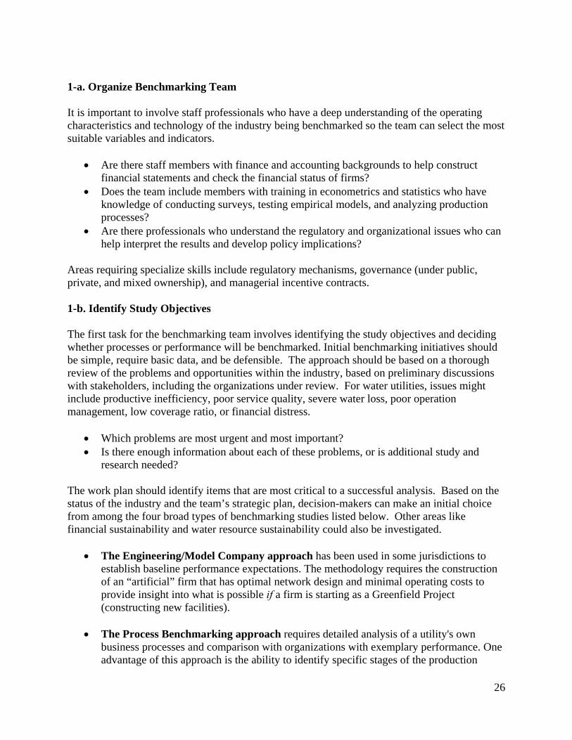
1-a. Organize Benchmarking Team It is important to involve staff professionals who have a deep understanding of the operating characteristics and technology of the industry being benchmarked so the team can select the most suitable variables and indicators.

• Are there staff members with finance and accounting backgrounds to help construct financial statements and check the financial status of firms?

• Does the team include members with training in econometrics and statistics who have knowledge of conducting surveys, testing empirical models, and analyzing production processes?

• Are there professionals who understand the regulatory and organizational issues who can help interpret the results and develop policy implications?

Areas requiring specialize skills include regulatory mechanisms, governance (under public, private, and mixed ownership), and managerial incentive contracts. 1-b. Identify Study Objectives The first task for the benchmarking team involves identifying the study objectives and deciding whether processes or performance will be benchmarked. Initial benchmarking initiatives should be simple, require basic data, and be defensible. The approach should be based on a thorough review of the problems and opportunities within the industry, based on preliminary discussions with stakeholders, including the organizations under review. For water utilities, issues might include productive inefficiency, poor service quality, severe water loss, poor operation management, low coverage ratio, or financial distress.

• Which problems are most urgent and most important? • Is there enough information about each of these problems, or is additional study and

research needed? The work plan should identify items that are most critical to a successful analysis. Based on the status of the industry and the team’s strategic plan, decision-makers can make an initial choice from among the four broad types of benchmarking studies listed below. Other areas like financial sustainability and water resource sustainability could also be investigated.

• The Engineering/Model Company approach has been used in some jurisdictions to establish baseline performance expectations. The methodology requires the construction of an “artificial” firm that has optimal network design and minimal operating costs to provide insight into what is possible if a firm is starting as a Greenfield Project (constructing new facilities).

• The Process Benchmarking approach requires detailed analysis of a utility's own

business processes and comparison with organizations with exemplary performance. One advantage of this approach is the ability to identify specific stages of the production

26

process that warrant attention to improve utility performance. According to IBNET, process benchmarking includes five steps, such as identifying key focus areas for comparison, gathering internal data for those key focus areas, identifying potential benchmarking partners, preparing for and undertaking benchmarking visits, and implementing best practices.

• The Performance Benchmarking (metric benchmarking) approach involves the

quantitative measurement of relative performance (cost efficiency, technical efficiency, scale efficiency, allocative efficiency, and efficiency change). Performance is compared with other utilities at a point of time and over time, using partial performance indicators or parametric and nonparametric frontier methods.

• The Customer Survey Benchmarking approach focuses on the perceptions of

customers as a key element for performance evaluation. Therefore, service quality is the core issue of this approach. For countries with poor customer service quality, this method might be useful in identifying problem areas and for establishing targets that provide incentives for firms to improve service quality.

1-c. Select Methodology and Refine Study Objectives After making the initial choice (here, assumed to be Performance Benchmarking), decision-makers need to focus and refine this choice to identify specific aspects of the practice they want to benchmark.

• To what extent are data on inputs, outputs, and environmental conditions available on a consistent basis across organizations?

• How do the performance comparisons relate to the final goal sought by those conducting the study?

To answer these questions, analysts need to have a clear idea of what kind of information they are seeking, what aspects of performance are likely to need improvement, and what targets for future performance might be most reasonable. For instance, if the analyst chooses to conduct a performance benchmarking comparison, he or she will need to decide the focus of the study:

• Are firms producing on the frontier—so no additional output could be obtained from the inputs? (technical or engineering efficiency)

• Is the right combination of inputs chosen to minimize costs? (cost or production efficiency)

• Is the quality of service consistent with customers’ willingness to pay (an element of allocative efficiency)

• Do prices reflect incremental production costs? (an element of allocative efficiency) • Are organizations operating where scale economies have been achieved? (scale efficiency) • Are organizations operating where economies of scope have been achieved (scope

efficiency reflecting multi-product economies, such as delivering water and wastewater services)

27

• Are there multiple issues to be addressed? (if so, such complexity is likely to require a combination of approaches)

Furthermore, analysts might be interested in the total factor productivity change (TFPC), which can be further decomposed into technical efficiency change, scale efficiency change, technology change, quality change, and allocative efficiency change. At this stage, analysts need to have clear objectives so appropriate data are collected and a suitable model can be specified. 1-d. Selection of Timeframe and Peer Comparison Group Based on the objectives, decision-makers then need to choose the timeframe and comparison group for the analysis. For instance, if the objective is to compare the relative efficiency of the water utilities in a particular year and the sample size is reasonable, analysts can conduct cross sectional analysis. If the objective is to evaluate the efficiency change of a single utility over time, analysts can use time series data from the utility. In this case, a partial indicator might be more suitable than frontier methods because of the limited sample size. If the objective is to evaluate both the current period relative performance and the TFPC, a panel data analysis is necessary, consisting of repeated observations on the same cross sections of firms over time. Regarding the selection of peer comparison groups, a number of options can be considered:

• Within-region Comparisons: A regional utility regulatory task force may want to compare the relative performance of the utilities within the region.

• Cross-region Comparisons: On the other hand, the regional group may want to compare the utilities within the region to the utilities in other regions to check for efficiency gaps.

• National Comparisons: Similarly, a national regulatory committee may want to conduct national or international benchmarking to evaluate the relative efficiency of domestic utilities or efficiency gaps between domestic and foreign utilities.

However, there are also potential obstacles and risks to conducting cross regional/international benchmarking.

• Data Availability: For a regional regulator, it might be difficult to get detailed information on utilities in other regions because the regulator/utilities in other regions may be reluctant to provide information.

• Data Consistency: Similarly, it might be difficult for the national regulatory committee to obtain consistent data from other countries.

• Exogenous Factors: A more important issue is the potential difference among the countries, such as geographical environment, population, weather, and past natural disasters.

• Accounting Definitions: Furthermore, there may be different accounting standards for international benchmarking.

If a regional/national regulator is not aware of these potential differences, the benchmarking results might be biased or incorrectly interpreted. For example, in the area of financial accounting, different countries may have different definitions of revenue, net income, operating

28

cost, capital expenditure, and depreciation, which might exert significant effects on the benchmarking results. Therefore, for international benchmarking, it is safer to use the physical inputs/outputs instead of monetary inputs/outputs. IBNet, IWA, and regional collaborative groups have a number of initiatives to improve data collection and reporting procedures. Overall, benchmarking at the local, national, and international levels helps all water and sanitation utilities identify and share best practice and new knowledge. Collaboration can promote the delivery of the best services for customers. Whatever their development status, groups can benefit from continuing professional education and cooperation. Regional and international initiatives facilitate the creation of international data banks that provide a productive environment for international benchmarking studies. However, it is important to pay attention to the potential differences among countries when conducting international benchmarking studies. 1-e. Gather Raw Data: Collection Issues After deciding the objectives and scope of study, the more comprehensive data collection can begin. Here we consider the main problems experienced by water utility companies in developing countries, which have generally experienced poor performance and low productivity. Risks associated with each problem will be identified to illustrate the tasks facing regulators, government ministries, operators, multilateral organizations, and private investors.10

Technical and Operational Problems:

• Inefficient operational practices (often reflecting poor governance systems), • Inadequate maintenance (stemming from under-pricing service in many jurisdictions), • High unaccounted-for water (caused by leakage and commercial losses—theft), • Limited service expansion (based on financial constraints), and • Inadequate water quality procedures (both for monitoring and producing potable water).

How does an outside analyst evaluate technical and operational risks associated with these problems? Unless the government-owned firm keeps adequate records there will be insufficient information about the state of installations and the need for replacement, rehabilitation, or expansion. Furthermore, operational performance of the system is questionable. How old are pipes and pumping devices? Have maintenance procedures been adequate in the past? What is the percentage of water not accounted for? What is the source of losses—leakage or commercial losses (theft)? What procedures are used to guarantee water quality? What is the level of operating costs? What are system expansion possibilities? Are water sources adequate? This litany of data questions illustrates the types of uncertainties facing those who analyze how inputs translate into outputs or production costs at different stages of production. Commercial and Financial Concerns: 10 Parts of this section draw upon Berg and Corton (2002), “Infrastructure Management: Applications to Latin America,” in Private Initiatives in Infrastructure: Priorities, Incentives, and Performance, eds. S.V. Berg, M. G. Pollitt, and M. Tsuji (Edward Elgar: Cheltenham, UK).

29

• Un-metered systems create distortions in consumer charges, • The amount of water produced is often estimated (instead of being based on actual

measurements), • Reliable consumption (or billing) data may be unavailable because of poor customer

recordkeeping, • Inefficient billing and collection practices lead to high levels of accounts receivable,

which translates into non-payments, • Laws may prohibit cutting off water services, dramatically reducing customer incentives

to pay bills, • Government agencies may not pay their bills, placing a burden on other customers to

cover costs, • Realized revenues may not be sufficient to generate funds needed to expand service and

protect water resources and the environment from contamination, • Tariff policies often do not reflect the true economic cost of future water supplies, and • Tariff structures with large cross-subsidies characterize many utilities (pricing below cost

leads to utility disincentives to serve those customers who are officially targeted as “worthy” of subsidization). Others end up benefiting from the subsidies.

Cost recovery cannot occur when there is such uncertainty regarding these aspects of operations. The baseline is always current procedures and capabilities, so if these are inadequate, organizational changes will be required. New administrative procedures are likely to be disruptive, requiring internal education and buy-in by current employees and customers. For example, what are the mechanisms for responding to customer complaints? Sometimes it is easier to start from scratch than to try to graft new systems onto old procedures. Similarly, historical records are required for making forecasts. How has demand evolved over time? Are the seasonal and hourly patterns predictable? In the area of financial risks, currency valuation and convertibility raise issues. Mechanisms for hedging risks have a high priority for external investors who need to be aware of government rules regarding remittances by foreign companies (and likely developments in this area).

Human Capital and Personnel Issues • Excess staff indicates poorly managed water utilities, • Political appointments and intervention are present in many nations, • There is often an inability to attract managerial talent and qualified technical staff due to lack

of adequate incentives (or caps on civil servant salaries), and • Frequent turnover of high-level staff combined with low productivity (and lack of discipline

in the labor force) present problems for managers. Regulatory monitoring by public agencies and due diligence by potential investors both require investigations into a number of issues, including the way contractual disputes are resolved:

• Is a union contract in place? • Have pension fund contributions been kept up?

30

• What is the managerial compensation scheme? • Are current managers the result of political appointments? • What is the turnover of staff at various levels of responsibility? • Are job descriptions flexible?

Most of these issues will not be revealed through statistical studies of relative performance, yet they have implications for the performance of the water utility.

Regulatory Governance and Incentives Issues Financial markets view the regulatory regime as a major determinant of the likely riskiness of cash flows. In addition, government funds have opportunity costs: education, health, transportation and other infrastructure areas compete with water utilities for funds. Private investors and firms with managerial contracts seek a number of features in the environment to insulate decisions from day-to-day politics, while ensuring long-run sustainability of the regime itself.11 Finally, multilateral organizations are hesitant to support water systems that have no prospects for performance enhancement (and the lack of data means that baselines cannot be developed). Output Based Aid from international funding organizations and national agencies is predicated on setting and meeting performance targets. Regulatory governance refers to the procedures used by the agency to conduct its activities, while incentives are the result of particular policies. Both are important, but the first provides a foundation for the latter. Appendix 1 (Variable Definitions) lists some variables that have been used in benchmarking studies to control for private and public ownership, regulatory incentives, and corporate governance. b. Step 2: Screen and Analyze Data Conducting a benchmarking study is an iterative process. Detailed screening of the data will result in greater refinement in the timeframe, sample size, and statistical techniques. The sub-steps of this second stage require more technical skills than the initial framing of the issues to be investigated. However, feedback should be elicited from those who participated in Step 1 so that there is agreement regarding decisions taken at this stage. After assembling the raw data, the benchmarking team should screen the data carefully to ensure the quality and quantity of information being gathered meet the requirements to allow for a successful project. This process is crucial to the study because poor data quality (inconsistent definitions, missing data or extreme data values) may lead to biased results. Insufficient data could result in the use of more limited models that might constrain functional forms so as to yield biased or skewed results. Figure 4 identifies four broad metric methodologies that might be utilized.

11King and Pitchford (1998) provide an overview of privatization issues.

31

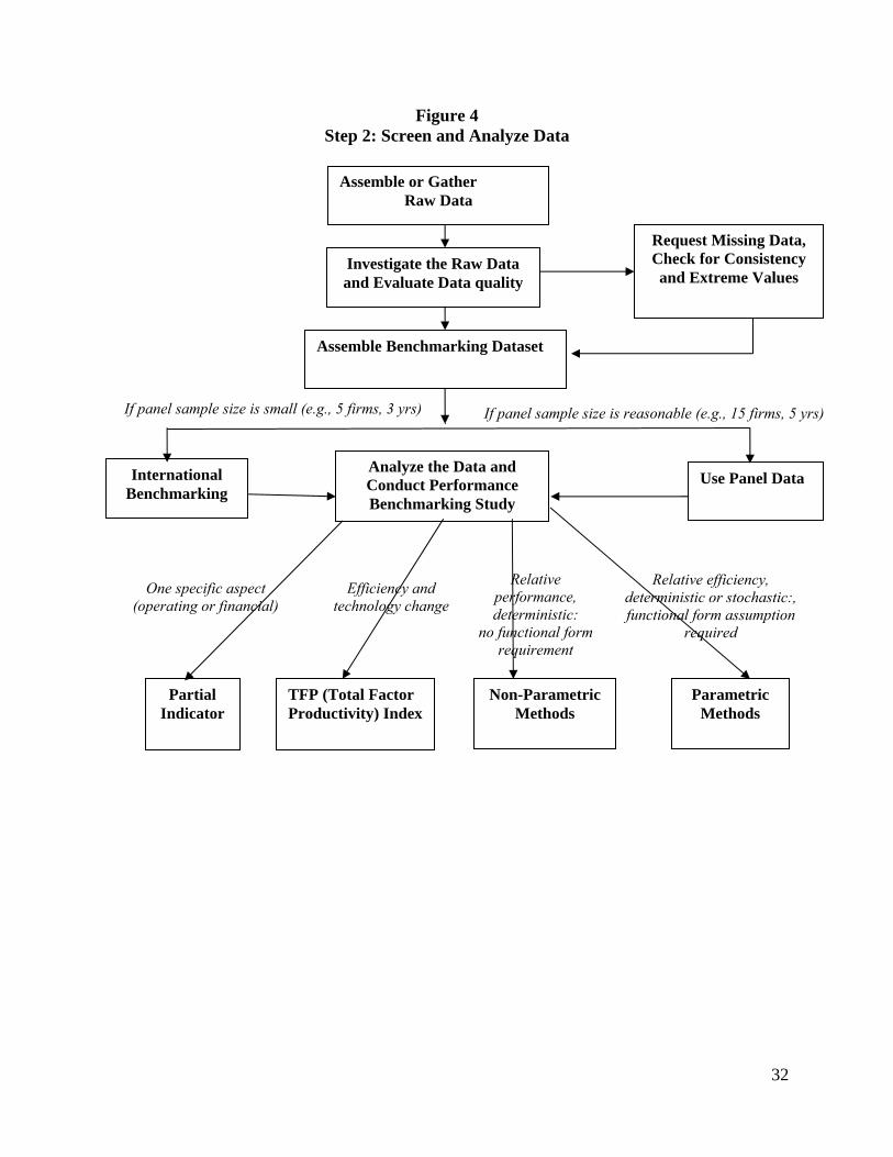
Figure 4 Step 2: Screen and Analyze Data

Investigate the Raw Data and Evaluate Data quality

Assemble Benchmarking Dataset

Analyze the Data and Conduct Performance Benchmarking Study

Partial Indicator

One specific aspect (operating or financial)

TFP (Total Factor Productivity) Index

Efficiency and technology change

Non-Parametric Methods

Parametric Methods

Relative performance, deterministic:

no functional form requirement

Relative efficiency, deterministic or stochastic:, functional form assumption

required

International Benchmarking

Assemble or Gather Raw Data

Request Missing Data, Check for Consistency and Extreme Values

If panel sample size is small (e.g., 5 firms, 3 yrs) If panel sample size is reasonable (e.g., 15 firms, 5 yrs)

Use Panel Data

32

Benchmarking is well developed on theoretical grounds and has an admirable objective. However, in practice, the results can be distorted. There are still many problems with the various methodologies: • Core Overall Performance Indicators (OPIs combine partial indicators of operating or

financial performance; these are summary indices), • Total Factor Productivity Indices (an index number approach that considers output per

unit input—where multiple inputs are taken into consideration to gauge efficiency levels and changes),

• Relative Performance using Data Envelopment Analysis (a non-parametric technique that makes no assumptions about the functional form of production or cost functions),

• Relative Performance using Statistical Techniques (parametric approaches that involve assumptions about functional relationships)

Each of the approaches has strengths and limitations. Some argue that the limitations of the methodologies supports postponing studies until the data can be fully audited and analysts achieve more agreement regarding which methodologies should be applied in particular circumstances. Others maintain that we can learn a great deal though preliminary analyses, and that the data collection effort will be strengthened by research initiatives. The authors of this Report are part of the second camp. 2-a. Investigate the Raw Data and Evaluate Data Quality Measurement is one of the first steps in the benchmarking process. Making comparisons requires significant amounts of data that are often quite difficult to collect. The results depend on the accuracy of the data that are collected. The information collected may be verified by the regulator (or analyst), but this usually comes at some cost. In addition, some data are unverifiable by the regulator or extremely costly to acquire. From this point of view, the regulator has to trust the firm regarding the truthfulness and accuracy of reported data on the operations of the utility: inputs, input prices, outputs (in volume and quality), revenues, and status of assets. The regulator cannot know for sure whether the reported operating expenditures and capital expenditures reflect the least cost for achieving reported outputs. We then end up in a situation of severe information asymmetry, which is the fundamental problem of regulation. Recall the principle behind benchmarking is that regulators cannot rely solely on the information provided by the firm when designing its regulatory framework (including targets and incentives). Since the utility benefits from having private information, regulators would like to avoid such dependence when designing targets for a rate-of-return-based price structure or a price-cap regime (including an X-factor). However, if a benchmarking methodology still requires information from the firm, one can argue that we have gained little by choosing this more sophisticated method. Furthermore, mismanaged water utilities are not likely to collect the relevant information needed for effective managerial decision-making—either because the managers lack the skills or because they do not want to document poor performance. Those entrusted with monitoring the utility may not do their jobs: Water Ministries and legislative committees (in the case of publicly

33

owned firms) may use utilities for political purposes, and have minimal incentive to collect accurate information regarding performance. Similarly, in the case of privately owned firms, the Board of Directors may have an underdeveloped internal governance system. Managers of both publicly- and privately-owned water utilities may present information in a selective manner to limit the impact of organizations providing oversight. After assembling the raw data, the benchmarking team should screen the data carefully to ensure the quality and quantity of information being gathered meets the requirements to allow for a successful outcome. This process is crucial to the study because poor data quality (including the presence of outliers) may lead to biased results. Specifically, attention must be paid to the following aspects when investigating raw data and their quality: Missing Data Missing data is a common problem for developing countries, which may pose a serious problem for the benchmarking study for the following reasons.

• Sample Size: Missing data will reduce sample size. As mentioned above, a reasonable sample size is necessary for conducting sophisticated frontier benchmarking models such as Data Envelopment Analysis (DEA) and Stochastic Frontier Analysis (SFA). This issue becomes one of the major obstacles for many developing countries when conducting these kinds of studies. Many countries only have data for a few water utilities covering a short time period (due to previous mismanagement). Missing observations further reduce what is often already a limited sample size, which makes sophisticated studies even more difficult.

• Nonrandom Missing Data: The missing data may be non-randomly distributed. For

example, data providers (utilities) could have accidentally forgotten to supply data-randomly distributed missing data; or they could have intentionally not provided the data because the observations might demonstrate poor operations. The nonrandom missing data will influence the statistical inferences because the observed sample will be a truncated sample of the true sample. Even for nonparametric models, deliberately withheld data will influence the benchmarking results because firms with poor performance might be omitted systematically from the sample.

Remedies: There are three ways to address the missing data problem: (1) Delete the observations with missing values for variables, (2) Estimate (impute) missing values using existing observations and then use the estimated

values in the data analysis, or (3) Ask the utility to provide the missing data. As explained above, option (1) will reduce the sample size and option (2) may be inappropriate where the missing data are not random. Therefore, option (3) is recommended since it will reduce the potential problems we mentioned above. Having an external (and independent) auditor assist in data collection can improve the process.

34

Accuracy and Comparability of Data Files Before moving into formal statistical analysis, it is helpful to engage in preliminary data checks of the computerized file: (1) Reduce data entry errors: Compare the computerized data set with the original data set to

make sure that the data have been entered correctly. (2) Prepare summary statistics: Summary statistics include the mean, median, standard

deviation, and minimum and maximum values of the key variables. Based on the summary statistics, analysts need to make sure that the utilities in the sample are really comparable to one another. For example, is utility A really comparable to utility B which is 100 times larger than A? Exclude the extreme case from the sample to make the sample more homogeneous and comparable.

(3) Calculate key ratios: Prepare summary statistics for key ratios such as water

delivered/employee and OPEX/water delivered. Pay attention to firms with extremely large or small ratios (those that deviate from the mean by more than 3-4 standard deviations). There might be some data input errors for these firms or they may have different organizational structures (e.g., outsourcing),

(4) Ensure comparability of data definitions: Check the definitions of the key variables to

make sure that they are really comparable. For example, does the number of employees refer to full time employees, part time employees, or total employees? Is the definition of operating cost similar across firms? In some cases, number of customers may not be a good output variable due to significant differences in service continuity. For instance, let company A’s number of customers be 1000 and average service time 4 hours/day. Company B’s number of customers is 600 and the average service time is 24 hours/day. In this case, the adjusted customer number (reflecting service hours) might be a better output measure, depending on the structure of the model.

(5) Recognize unique events or characteristics: Some special events such as natural disasters

may have significant impacts on operating costs and service quality indicators. If the impact is severe, it is better to exclude the observation from the sample in that year. Similarly, a utility located near a water source and one requiring substantial investments in water storage and transport will have different costs. Such differences should be incorporated into the analysis.

2-b. Assemble Benchmarking Dataset After investigating the data, the benchmarking team can assemble the benchmarking dataset. However, the sample size may not be large enough for utilizing sophisticated frontier models. Issues include model specification (and degrees of freedom) and ways to expand the sample size. Model Specification and Degrees of Freedom: For example, when comparing the relative efficiency of 10 utilities in a specific year, a translog production frontier with three inputs might

35

be used (specific functional forms are described below). These inputs could be labor, capital, and energy. Due to the translog functional form, there will be 9 regressors, which leaves very few degrees of freedom for the estimation. To solve this problem, a simple function form should be used (e.g., a log-linear Cobb-Douglas functional form). However, the trade-off is that Cobb-Douglas would impose more assumptions, such as the same production elasticities, the same scale elasticities, and unitary elasticities of substitution for all firms. Expansion of Sample Size: Another way around this problem is try to augment the sample size. There are two options available: use the panel data or conduct the international (cross regional) benchmarking. However, as was noted above, international (cross regional) benchmarking is risky due to the potential differences in accounting standards, economic conditions, and geographical environments. Therefore, the benchmarking team should first consider the panel data sample. If the panel data sample is still not large enough, international (cross regional) benchmarking can be considered. 2-c. Analyze the Data and Conduct Performance Benchmarking Study The process of model specification and technique selection process depends on benchmarking objectives, data availability, and the team’s willingness to adopt specific assumptions for each type of model. Hence, the benchmarking team may need to draw upon professional consultants or specialists at research institutions before moving to more sophisticated models. Two broad approaches to quantifying performance are outlined here: Data Envelopment Analysis: DEA is a method in which linear programming techniques are applied to a selected set of variables to calculate an efficiency coefficient for each water utility. The framework has been adapted from the multi-input, multi-output production and functions. The production function is a basic concept in economics used to determine how much output can be produced with a given basket of inputs. A cost function relates total cost to input use and input prices. DEA develops a function whose form is determined by the most efficient producers. This method differs from OLS that would base comparisons with respect to an average producer. DEA benchmarks firms only against the best producers (so it is a non-parametric frontier analysis). It can be characterized as an extreme point method that assumes that if a firm can produce a certain level of output utilizing specific input levels, another firm of equal scale should be capable of doing the same. The most efficient producers can form a “composite producer,” allowing an efficient solution for every level of input or output. Where there is no actual corresponding firm, “virtual producers” are identified to make comparisons. DEA is a non-parametric approach to evaluating performance: functional forms are not specified, although the type of returns to scale is incorporated into the model. DEA has been used for both production and cost data. Utilizing the selected variables, such as unit cost and output, DEA software searches for the points with the lowest unit cost for any given output, connecting those points to form the efficiency frontier. Any company not on the frontier is considered inefficient. A numerical coefficient is given to each firm, defining its relative efficiency. Different variables that could be used to establish the efficiency frontier are: number of employees, service quality, environmental safety, and fuel consumption. A recent survey of studies of electricity distribution companies identified more than thirty DEA analyses—

36

indicating widespread application of this technique to that network industry.12 Less than five such studies have been published for water utilities. The main advantage to this method is its ability to accommodate a multiplicity of inputs and outputs. It is also useful because it takes into consideration returns to scale in calculating efficiency, allowing for the concept of increasing or decreasing efficiency based on size and output levels. A drawback of this technique is that model specification and inclusion/exclusion of variables can affect the results. Statistical Analysis: Linear regression analysis seeks to derive a linear relationship between firm performance and market conditions and characteristics of the production processes. Other specifications (and/or data transformations) can capture non-linearities. Statistical analysis of production relationships can isolate the effects of specific conditions or input levels on the level of output—so the roles of multiple independent variables can be determined. Data from the firms being compared can then be used to calculate expected output, given the model coefficients and values of variables for each firm. The process is similar for a cost function. A major advantage of this method is its ability to reveal information about cost structures and distinguish between different variables’ roles in determining cost. Predicted versus actual cost can provide a measure of relative performance. The sensitivity of these results to changes in model specification or data points can then be examined to provide the policy-maker with a framework for evaluating firms. Econometric analyses have two major disadvantages. First, a large data set is necessary for reliable results. Obtaining the number of observations needed to derive an efficient and unbiased estimate of cost (or production) structures can often prove to be a difficult task. The second disadvantage is a statistical one. The regression results are sensitive to model specification (for example, a linear vs. a non-linear functional form). In addition, for some models, the interpretation of the error term becomes important. Nevertheless, these techniques are widely used to analyze other network industries. Appendix 2, an Annotated Bibliography of Water Benchmarking Studies, identifies over thirty statistical studies for the water sector.

The early studies tended to utilize Ordinary Least Squares (OLS) to estimate cost functions for firms. Due to data limitations, most of these studies were cross-sectional in nature. Besides using data from only a single year researchers utilized data from England and Wales or from the United States. These academic studies often focused on the relative performance of private vs. publicly-owned water and sewerage utilities. In addition, they investigated the extent of scale economies and economies of joint production (providing both water and sewerage services). In some cases, they considered the impacts of residential vs. industrial/commercial customers.

As data from Brazil, Peru, and other emerging nations became available, additional country studies were published—often using more advanced econometric (parametric) or non-parametric data analysis techniques. Studies of utilities in France, Italy, and other nations began to appear in the academic literature. Techniques associated with Stochastic Frontier Analysis began to be applied to both production functions and cost functions. Panel data facilitated the incorporation of customer density, topology, and other variables.

12 Jamasb, T. J., Pollitt, M. G. (2001). “Benchmarking and regulation: international electricity experience.” Utilities Policy, 9 (3), 107-130.

37

In addition, a number of cross country studies have been conducted by researchers at the World Bank. These studies characterize production processes in a region and to draw conclusions about the impacts of different institutional features (such as the presence of good governance procedures, the regulatory environment, and public/private ownership). Furthermore, quality of service has begun to be incorporated in empirical studies, through the use of hedonic output measures (adjusting the output for quality) or as separate outputs altogether (in multi-output models).

For this sub-step, we have already assumed that the benchmarking team is conducting a Performance Benchmarking Study (rather than one involving engineering models, process benchmarking, or customer service benchmarking). The team still needs to select from among four types of techniques, based on performance benchmarking objectives and data availability. The benchmarking team can choose one or more types of techniques for the study. The four options are partial indicators, TFP (total factor productivity) indicators, non-parametric methods, and parametric methods13. We will briefly discuss the data requirements, advantages, and disadvantages for each type. The discussion of specific sub-type techniques (Step 3) are also incorporated in this discussion. More comprehensive discussions of the techniques are presented in the Appendix 3: Technical Features of Benchmarking Methodologies. (1) Partial Indicators (Specific Core Indicators). Partial indicators (PIs) can provide a useful

starting point for identifying poor performers. Such “core indicators” include accounts receivable rates, cost recovery rates, water loss rates, or volume delivered per worker; these ratios can be used to capture specific aspects of utilities’ operating and financial performance. Simple trend analysis can draw a rough picture of firm performance change over time. Such indicators are sometimes combined to create an Overall Performance Index. • Data requirements: relevant variables used in the calculation of the ratios. • Advantages: PIs are easy to calculate; results are intuitive; the analyst can conduct a

comparison with only two observations. • Disadvantages: PIs only reflect one aspect of firm’s operating or financial activities; the

comparisons do not control for the impacts of other factors. When they are aggregated into an Overall Performance Index, the weights applied to each component are often not based on explicit policy priorities.

Total Factor Productivity (TFP) Index. TFP indices focus on the productivity change over time. Two commonly used TFP indices are the Tornqvist and Malmquist indicators.

(2) Tornqvist Index:

• Data requirements: quantity and price data on inputs and outputs for two or more firms or time periods.

• Advantages: not difficult to calculate; prices are used as weights; captures allocative efficiency; analyst can conduct a study with only two observations.

• Disadvantages: need price information for inputs and outputs; TFP change cannot be

13 Coelli et al. (2003) summarize some of these issues in Table 2.3 of their book “A Primer on Efficiency Measurement for Utilities and Transport Regulators.”

38

further decomposed into technical efficiency change, technology change, and scale efficiency change.

(3) Malmquist Index:

• Data requirements: only quantity data on inputs and outputs for firms in different time periods.

• Advantages: price information not needed; based on DEA model, so no functional form assumption; TFP change can be decomposed into technical efficiency change, technology change, and scale efficiency change.

• Disadvantages: needs relatively large sample size for each time period; the panel has to be balanced (same firms appear in every period).

Nonparametric Methods: The most commonly used non-parametric methods are Data Envelopment Analysis (DEA) and related models. DEA is a linear programming method that constructs a nonparametric production frontier by fitting a piece-wise linear surface over the data points. The technical-efficiency based DEA models can be constant returns to scale (CRS) and/or and variable returns to scale (VRS) models. Other DEA models include DEA with preference structure, DEA with undesirable outputs and DEA with environmental variables.

(4) DEA Production Returns to Scale models. DEA models can be specified to be Constant or

Variable Returns to Scale.

• Data requirements: only quantity data on inputs and outputs for the sample of cross-sectional firms or the panel. The panel sample does not need to be balanced.

• Advantages: no functional form assumption; can easily handle multiple inputs and outputs.

• Disadvantages: requires relatively large sample size; attributes all the deviations to inefficiency (no random noise); as the complexity (number of variables) in a DEA model increases, the discrimination power of DEA models decreases; more firms tend to be on the efficiency frontier.

(5) Cost efficiency DEA model. If price information of the inputs is available, the analyst can conduct a cost efficiency DEA model to calculate the cost efficiency of the firms. Since cost efficiency is the product of technical efficiency and allocative efficiency, the analyst can calculate firm-specific allocative efficiency based on the cost efficiency DEA model and regular VRS/CRS DEA models.

• Data requirements: quantity data on inputs and outputs and price data on inputs for

cross-sectional firms or panel sample; panel sample does not need to be balanced. • Advantages: can be decomposed into allocative efficiency, technical efficiency, and

scale efficiency. • Disadvantages: same as those listed for CRS/VRS DEA models; it is often difficult to

obtain input prices.

(6) Super efficiency DEA model. Results may yield multiple efficient utilities (efficiency

39

score=1) in the CRS/VRS models. This outcome is especially likely if the sample size is small relative to the number of variables used in the DEA models. The super efficiency model is one method used to rank the efficient utilities. The basic idea of super efficiency model is to compare the efficient firm to the frontier constructed from all other firms (excluding the firm itself) and evaluate the relative efficiency superiority of the firm to the others.

• Data requirements: quantity data on inputs and outputs for cross-sectional firms or panel

sample; panel sample does not need to be balanced. • Advantages: can rank the efficient utilities in CRS/VRS models. • Disadvantages: the firms are not compared to the same “standards” because the frontier

constructed from the remaining firms changes for each efficient firm being evaluated.

Parametric Methods. The most commonly used parametric methods are Stochastic Frontier Analysis (SFA) and corrected ordinary least squares (COLS) models. The main difference between these models is that COLS attributes all the deviations to inefficiency while SFA models attribute part of the deviations to inefficiency and part of the deviations to random noise. In other words, the SFA models take both inefficiency and random noise into account. The most widely used stochastic frontier models include the stochastic production frontier model, stochastic cost frontier model, and stochastic distance function model. Before selecting a specific model, analysts have to make an initial choice between the two most widely used functional forms: Cobb-Douglas function and translog function.

Cobb-Douglas: An obvious advantage of Cobb-Douglas functional form is that it requires the estimation of very few parameters (for instance, four in a Cobb-Douglas production function with three inputs). Furthermore, the coefficients are very easy to interpret. However, the Cobb-Douglas assumes that all firms have the same production elasticities, the same scale elasticities, and unitary elasticities of substitution; these assumptions are quite strong. Translog: By comparison, the translog functional form is the most commonly used flexible functional form. While it requires the estimation of many more parameters than the Cobb-Douglas (for instance, fourteen in a translog production function with three inputs and time trend variable), it does not impose the restrictions imposed by the Cobb-Douglas. Another advantage of using translog function is that the practitioner can decompose the TFP change into the technical efficiency change, technology change, and scale efficiency change. Therefore, it is generally more preferable to use the translog functional form. However, the translog function requires a relatively large sample size and more complicated estimation process, such as imposing the assumption that the function is homogeneous of degree one in input prices and/or joint estimation of first-order cost share functions. Therefore, for analysts with very limited sample size and experience, it is better to start with the Cobb-Douglas functional form. After accumulating the data for additional years and gaining experience over time, the regulator can consider utilizing the translog functional form.

(7) Stochastic Production Frontier model: The Stochastic Production Frontier describes output (e.g., water delivered) as a function of inputs (e.g., capital, labor, energy). The difference between the actual output and estimated (predicted) output is attributed to inefficiency and

40

random noises.

• Data requirements: quantity data on inputs and outputs for cross sectional firms or panel sample. The panel sample does not need to be balanced.

• Advantages: no need for price information; efficiency change can be decomposed into technical efficiency change, technology change, and scale efficiency change.

• Disadvantages: only one output can be taken into account; there is a potential endogeneity problem because input factors in a production function might be jointly determined with the output produced.

(8) Stochastic Cost Frontier model: Stochastic Production Frontier describes cost as a function of input prices and outputs. Difference between the real cost and estimated cost is attributed to inefficiency and random noises.

• Data requirements: quantity data on inputs and outputs and price data on inputs for cross sectional firms or panel sample; the panel sample does not need to be balanced.

• Advantages: can take multiple outputs into accounts; no potential endogeneity problem; efficiency change can be decomposed into cost efficiency change, technology change, and scale efficiency change; can calculate the allocative efficiency change if the results of the Tornqvist index are combined.

• Disadvantages: might be difficult to get accurate input prices. (9) Stochastic Frontier Distance Function Model: A distance function may have either an input or an output orientation. An input orientation looks at how much the input vector may be proportionally contracted, holding the output vector fixed; an output orientation looks at how much the output vector may be proportionally expanded with the input vector held fixed. The distance function can be thought of as a multiple output version of a production frontier.

• Data requirements: quantity data on inputs and outputs for cross sectional firms or panel sample; the panel sample does not need to be balanced.

• Advantages: takes into account multiple outputs and inputs simultaneously; no need for price information; no assumption about the cost minimization; avoids the potential endogeneity problem in production function; efficiency change can be decomposed into technical efficiency change, technology change, and scale efficiency change.

• Disadvantages: relatively strong assumptions of the distance functional form, difficult to interpret the coefficients.

(10) Corrected Ordinary Least Squares: Similarly, the COLS approach includes production function and cost function options.

• Data requirements: quantity data on inputs and outputs for production function; quantity data on inputs and outputs and price data on outputs for cost function.

• Advantages: easy to calculate, estimation is based on Ordinary Least Square (OLS); results are generally close to SFA models; can be used for robustness checks.

• Disadvantages: assumes all the deviations are due to inefficiency.

41

42

(11) Fixed or Random Effects Models (Distribution Free Methods): The most widely used distribution free models are fixed effect and random effect models. These two models do not impose specific distribution assumptions onto the inefficiency terms, whereas in the stochastic frontier models the inefficiency term is assumed to follow specific distributions such as exponential, half normal and truncated normal distributions. However, each of these methods has its own limitations.

Fixed effects model: Assume the inefficiency term is captured by the time-invariant inefficiency term in fixed effect model. Firm-specific intercepts are estimated and the exponential term of the difference between the firm-specific intercept and the largest intercept among all the firms is regarded as the firm specific efficiency score.

• Data requirements: quantity data on inputs and outputs for production function; quantity

data on inputs and outputs and price data on outputs for cost function. • Advantages: no distribution assumption of the inefficiency term; easy to estimate. • Disadvantages: imposes strong assumption that the inefficiency is time invariant; the

fixed effect (time invariant unobserved term) captures not only the inefficiency but also the effects of all phenomena (such as regulatory environment, ownership) that vary across utilizes but that are time invariant to each utility.

Random effects model: Random effects models relax the assumption that inefficiency is time invariant. In the random effect model, inefficiency terms are assumed to be randomly distributed with constant mean and variance, but are also assumed to be uncorrelated with the other regressors (in fixed effect models, inefficiency terms are allowed to be correlated with the other regressors). Firm-specific efficiency is estimated as the exponential form of difference between the average firm-specific residuals over time and the largest average firm-specific residual among the sample.

• Data requirements: quantity data on inputs and outputs for production function; quantity

data on inputs and outputs and price data on outputs for cost function. • Advantages: no distribution assumption of the inefficiency term, allows the presence of

time-invariant regressors. • Disadvantages: imposes the strong assumption that the inefficiency term is not

correlated with the other regressors; the estimation may be biased if the time period is very short.

These eleven analytic techniques illustrate the range of methodologies available to those examining the determinants of utility output and utility costs. Since the resulting performance scores are only as accurate as the underlying models, the application of these approaches requires substantial technical skill.

43

Fixed/ Random Effects

Figure 5 Step 3: Utilize Specific Analytic Techniques

Summary Indices (e.g.,

Output per worker)

Tornqvist Index

Malmquist Index

Quantity and price info for output and

inputs

Only have quantity info

DEA Production

Scale (CRS & VRS)

Quantity info return

to scale

DEA Cost

Efficiency Model

Info on input prices and

output quantity

DEA Super

Efficiency Model

Rank “efficient”

firms

SFA Production Function

Quantity info single output

SFA Cost

Function

Input prices and output quantity

Multiple outputs

SFA Distance Function

COLS Corrected

OLS

Deterministic Distribution free, assume

time invariant inefficiency

Parametric Methods

Alternative Inputs and Outputs (e.g., network length vs. fixed assets; quality as an output)

Sensitivity Tests:

Model Specification (e.g., translog vs. log-linear)

Alternative Methodologies (e.g., DEA vs. SFA)

Non-Parametric Methods

TFP (Total Factor Productivity)

Index

Partial Indicator

Ratios: Partial Metrics

c. Step 3: Utilize Specific Analytic Techniques

In many cases, research raises more questions than it answers. Public policy-makers would like empirical studies to answer questions that have decision-relevance. The publications and studies summarized in the Technical Appendices have primarily involved academic researchers, sometimes in the context of rate cases—or as a retrospective look at how methodologies were used by regulators. Consulting firms have entered the fray, as well. Water utility managers are likely to fear the misuse of empirical studies: they tend to prefer process benchmarking studies that can identify changes in specific practices that would improve performance.

Note that some economists are skeptical of benchmarking studies. Shuttleworth14 argues that total factor productivity approaches may be superior to DEA and SFA approaches to benchmarking: “Benchmarking may still have a role to play in regulation, as long as regulators recognize that the residual merely measures the extent to which the model has failed to explain costs, and not the extent to which companies are inefficient. Stable and predictable regulatory techniques have to rely on other forms of evidence.” (p. 317) However, in the same issue of Utilities Policy, Burns, Jenkins, and Riechmann15 are much more positive regarding the benefits associated with benchmarking studies. They note that the different methodologies differ in assumptions, in their ability to discriminate between the impacts of different explanatory variables, and the importance of selecting appropriate variables. However, they argue that benchmarking studies can be valuable for regulators. Shuttleworth also finds that benchmarking can help in the following cases: • “To decide which companies out of a large sample deserve closer (and more objective)

examination, so that scarce investigative resources are allocated efficiently; • To appraise individual cost items, if their cost drivers are a matter of consensus; • As a preliminary step in the detailed investigation of each company’s costs, aimed at

identifying decisions that should be investigated further for ‘imprudence’.” (p. 317) Overall, the process of model specification and technique selection process is not easy. The outcome depends on benchmarking objectives, data availability, team capabilities (and resources), and the team’s willingness to adopt specific assumptions within each type of model. Hence, the benchmarking team may need to consult professional consultants or specialists at research institutions before moving to the more sophisticated model. The detailed discussion of Step 2 outlined the strengths and limitations of the different analytic techniques:

Partial Indicators (1) Summary Indices (Core Indicators) Total Factor Productivity (2) Tornqvist Index

14 Graham Shuttleworth (2005) “Benchmarking of Electricity Networks: Practical problems with its use for regulation,” Utilities Policy, Volume 13, No. 4, pp. 310-317. 15 Phil Burns, Cloda Jenkins, Christoph Riechmann (2005). “The role of benchmarking for yardstick competition,” Utilities Policy, Volume 13, No. 4, pp. 302-309.

44

(3) Malmquist Index Nonparametric (4) DEA Production Scale (5) DEA Cost Efficiency (6) DEA Super Efficiency Parametric (7) SFA Production Function (8) SFA Cost Function (9) SFA Distance Function (10)Corrected Ordinary Least Squares (COLS) (11)Fixed and Random Effects Models

These methods are arrayed in terms of the technical quantitative skills required for implementing the different approaches. Availability of software and specialized skills can be as important as data availability in determining the types of models utilized. Summary indices allow analysts to review trends of core indictors over time. Total factor productivity indices provide more comprehensive characterizations of trends over time and of relative performance across a set of water utilities. However, these (and parametric and nonparametric methods) may not incorporate a number of important dimensions of performance noted above (e.g., financial sustainability or some aspects of customer service or water quality—due to difficulties in incorporating these factors into DEA, SFA, or COLS models. Thus, more sophisticated techniques are not necessarily the most useful in the context of benchmarking. Sometimes simple partial indicators can provide useful comparisons that are intuitive. In addition, credible performance comparisons require that the results be communicated in a manner convincing to stakeholders. d. Step 4: Sensitivity Tests In making performance comparisons through benchmarking analyses, the analyst is interested in obtaining a measure of firms’ relative efficiency. Such information can be used to develop X-factors in price cap regulation, to reward (or punish) companies. Or the regulator might want to publish the rankings or efficiency scores to provide the public with information, putting pressure on managers of poor performing utilities to improve the performance of their firms. In both cases, the accuracy and robustness of inefficiency estimates are very important because they may have significant financial or social impacts. In particular, if the estimated inefficiency scores or rankings are sensitive to the benchmarking method, a more detailed analysis is required to justify the adopted model. Tests for mutual consistency are becoming standard. . Nevertheless, in most cases there is no ‘‘ideal’’ model among the set of potential models. Issues include model specification (cost vs. production and functional form), alternative specification of inputs or outputs (e.g., network length vs. fixed assets as an input), assumptions about error terms, and alternative methodologies (e.g., DEA vs. SFA). Following the work of others, we suggest three levels of sensitivity tests.

45

To check for the robustness of performance rankings, researchers have begun to compare results from different methodologies: using correlation matrices or verifying whether different models identified the same set of utilities as the most efficient and least efficient firms. Clearly, if efficiency scores are to have any use for managerial incentive or as elements in regulatory mechanisms, stakeholders need to be confident that the scores reflect reality, and are not just artifacts of model specification, sample selection, treatment of outliers, or other steps in the analytic process. Thus, analysts are performing sensitivity tests. Benchmarking methodologies can produce dramatically different results under similar circumstances. A quick review of the benchmarking literature reveals that conclusions (such as performance rankings or scores) differ considerably, depending on the

• variables chosen, • the particular methodology applied, • the interval of time considered, and • other factors that need to be determined for a benchmarking study.

This point applies to all the methodologies used: from simple ratio analyses to sophisticated quantitative techniques (such as ordinary least squares, stochastic frontier analysis, Data Envelopment Analysis, and distance functions). This observation raises questions about how reliable a benchmarking process can be, especially when we realize that performance comparisons affect the economic foundations and financial sustainability of a company that is usually the sole provider of WSS service in a particular geographic area. This important issue brings into question the use of complicated mathematical techniques that are sensitive to manipulation. Bauer et al. (1998) propose a series of criteria that can be used to evaluate whether the results obtained from different methods are ‘‘mutually consistent,’’ that is, if they lead to comparable inefficiency scores and rankings. We will discuss these criteria in detail in the next step. Coelli and Perelman (1999) have suggested combining the results from alternative modeling exercises by using the geometric means of the performance scores for each data point in order to reduce potential bias. Thus, attention should be paid to the sensitivity of the results to the following elements:

• Model Specification (e.g., translog vs. log-linear) • Alternative inputs/outputs (e.g., network length vs. fixed asset) • Alternative methodologies (e.g., DEA vs. SFA)

Figure 6 identifies the Three Levels of Sensitivity Tests used to determine confidence in the performance comparisons.

46

Figure 6

Step 4: Sensitivity Tests

Level 1: Sensitivity tests of efficiency scores

Level 3: Sensitivity tests for

distinguishing best/worst

Level 2: Sensitivity tests of efficiency

rankings

Sensitivity Tests

Analyze the Scores and Rankings

Explore the Potential Determinants of Inefficiency

Summary statistics, t-test, Wilcoxon test, second stage regression, etc.

Evaluate Results Unacceptable

Portion of the Study is Inconclusive

Acceptable

47

4-a. Three Levels of Sensitivity Tests:

A problem faced by regulators willing to apply frontier studies is the variety of alternative model specifications and methodologies available. The problem becomes even more serious if different methods generate substantially different results. In an attempt to alleviate this problem and establish the conditions under which benchmarking results are most informative to regulatory committees, Bauer et al. (1998) proposed a set of consistency conditions when different measures are adopted by regulators., They find that the different methods used should provide consistent efficiency levels and rankings, and identification of best and worst performers, and also be consistent in results over time. We summarize their approach into three levels of consistency tests. Level 1: Sensitivity tests of efficiency scores. Pearson correlation matrix can be employed to check the correlation of efficiency scores between pairs of techniques. Furthermore, Kruskal-Wallis nonparametric test can be used to test the null hypothesis that different techniques generate the same distribution of efficiency scores. Level 2: Sensitivity tests of efficiency ranking: If the efficiency scores are not consistent across the different methods, it is still possible that these approaches generate similar rankings of firms by their efficiency score. A clear ranking can help a regulator determine the X factor to be used in setting prices for the firms in the sector. Thus, nonparametric Spearman’s ranking correlation matrix can be used to check the correlation of rankings between pairs of techniques. Level 3: Sensitivity tests of efficiency ranking: If the consistency in efficiency level and rankings was not met, it is still possible that these approaches can identify the best and worst performers, which can be especially helpful for rewarding the best performers and punishing the worst performers. Therefore, the regulator can compare rankings yielded under the different techniques and summarize the overlapping rate of identifying the best and worst performers. After the three levels of tests, the regulator should have a good sense of the consistency of different methods. The regulator should pay more attention to firms that have similar efficiency scores/ranking under different approaches (for instance, a firm which is recognized as one of the worst performers by 3 different techniques). If the results are close to each other, we can calculate the geometric means of the efficiency scores for each firm to get a “comprehensive” efficiency measure. If there is substantial variance in all three level tests, the findings would be considered inconclusive; requiring a more detailed analysis to explore problems with the adopted models. 4-b. Analyze the Scores and Rankings and Explore the Potential Determinants of Inefficiency If the results pass the sensitivity tests, the benchmarking team can start to analyze scores and rankings and explore the potential determinants of inefficiencies across firms and over time. The utilities can be divided into different groups by various factors, such as regions, population density, regulatory environment, ownership structure, and vintage to compare the efficiency scores. Second stage regressions (OLS or Tobit) with the efficiency score as the dependent

48

variable can also be used to test the partial effects of these external factors on the firm efficiency. Firms should not be ranked as poor performers if they operate under conditions that differ from those of the other firms. As noted earlier, density, geographic topology, distance from raw water sources, and political constraints on prices (affecting the financial sustainability of operations) affect relative performance. Given the complexity of benchmarking studies, it is useful to seek public comments that provide feedback, both augmenting the effort to analyze performance and promoting transparency and the legitimacy of the process. Exploring the potential determinants of inefficiency might require public workshops. It will certainly require participation of stakeholders. As has been noted before, utility managers have access to far more detailed information regarding production processes, opportunities for improvements, and costs associated with different strategies for cost containment, quality of service improvements, and other activities. Thus, performance rankings should not be viewed as ends in themselves. Rather, they are catalysts for promoting critical thinking about the sources of inefficiency. Figure 7 identifies steps in this process. e. Step 5: Develop Policy Implications The reason for resolving the methodological issues is to enable the analyst (and those using the study) to have confidence in the performance evaluation. Policy implications depend on how well the methodologies meet the principal criteria for choosing a set of performance measures: they have to be comprehensible, comprehensive, useable, and timely. We return to these issues later in this report. For now, Consider Figure 7:

49

Figure 7

Step 5: Develop Policy Implications

Explore the Potential Determinants of Inefficiency Lack of incentive regulation Obsolete technology and production processes Weak corporate governance and monitoring Inappropriate managerial incentive contracts Ownership structure (public vs. private) Other environmental effects (e.g., geography, topology)

Summarize the results

Suggestions/Strategies for Potential Improvement

(charts, tables, graphs, reports)

Seek Public Comments Prepare Follow-up

Benchmarking Studies

50

5-a. Explore the potential determinants of inefficiency Through the summary statistics and second stage regressions, the benchmarking team can identify the potential determinants of firm inefficiency, which might include but are not limited to the following factors:

• Lack of incentive regulation • Obsolete technology and production processes • Weak corporate governance and monitoring • Inappropriate managerial incentive contracts • Ownership structure (public vs. private) • Other environmental effects (e.g., geography, topology)

A detailed discussion about the definition, measure, and potential impacts of these factors is presented in Appendix 1: Variable Definitions and Explanations. 5-b. Summarize the Results: Formats for Presenting Comparisons

Any classification scheme can be misapplied. If the user does not have confidence in the scores or the rankings, then the studies will not be applied in the evaluation process. Some formats are described below to illustrate how studies have tried to present information in a useful manner. Tables: The simplest ranking scheme involves a table that ranks firms from strongest to weakest. The tables can group the water utilities into categories, directing attention to the firms that are most efficient and to those with the weakest performance. In all likelihood, the order of ranking and the “scores” will not be precise, so grouping allows the performance evaluator to acknowledge that no methodology is perfect. Reporting a score of 87.352 involves misplaced concreteness. No such score is likely to have so many significant digits, and even if one model did yield such an indicator, other methodologies would yield other “numbers”. In partial response to this issue, in Peru, SUNASS gives each municipal water utility a “grade”: for example, a C+ or A. This format provides an intuitive and easy-to-grasp measure of relative performance. In addition, it is possible for all the utilities to earn an A’s. Coefficients (and Scores) from DEA and SFA Studies: We have seen how quantitative studies can be very complicated, and the results may not appear to be very intuitive. For specialists, drawing conclusions about economies of scale or the association between service quality and costs involves careful specification and sensitivity tests. Presenting scores to non-specialists (based on the results of such studies) presents a challenge for econometricians. This area is one warranting much more attention, since different audiences require different types of reports. Fingerprint Charts: Another format allows an individual utility to be compared with another firm and/or with the average of a set of peer utilities. Peter Stahre and Jan Adamsson utilize six indicators: • Customer satisfaction—Performance indicators and measuring methods reflecting the

customers expectations and appraisal of the water services.

51

• Quality—Quality-related performance indicators complementing the economic indicators and the customer satisfaction indicators.

• Availability—Performance indicators describing the reliability of the entire system’s operations.

• Environment—Performance indicators illustrating the utilities’ environmental achievements.

• Organization/Personnel—Performance indicators describing efficiency and the relationship between "in-house work" and external services.

• Economy—Performance indicators comparing costs on an overall level. Figure 8 (taken from their study) illustrates one format used to compare the distribution network in the city of Malmo in relation to the calculated average situation in the 6-cities Group16:

“The general principle of the diagram is that the longer the “beams”, the worse are the conditions. Obviously, this is not the case for describing the age structure of the pipe network, which is marked in a deviant way. The fingerprint model is intended for benchmarking water distribution networks in different cities. For this purpose the information must first be normalised. The dotted line in the diagram (= 100%) represents the mean values of the respective parameters within the compared group of cities. The “fingerprint” represents the situation in one city and indicates how this city is positioned in relation to the calculated mean value for the group. The information in the diagram is thus given in percentage of the average.”

The format allows one to see key features of the network in a relatively compact way. “Every increment is 20%. The average in the 6-cities group is indicated by the dotted line (= 100 %). The average in absolute numbers is given in parenthesis for every parameter.” In general, the tighter the “star”, the better, except for the “share of network” elements which help the analyst understand the relative age of the networks. Other factors, such as soil conditions or topology, could be incorporated into the comparison. The fingerprint model is particularly useful for characterizing multidimensional “core performance indicators” of a pipe network. However, it is probably more useful for professionals than for the average citizen.

16 Paul Stahare, Jan Adamsson, (2002). Performance Benchmarking – A powerful management tool for water and wastewater utilities, , Suecia.

52

Figure 8. Characteristics of the Water Distribution System of Malmo

(5.67) O&M costs (Euro/m pipe)

(0.743)Complaints (number/1000

subscribers per year)

(0.143)Water leaks

(no/km/year)

(220) Renewal rate

(years)

(28.1) Capacity utilisation (billed m3/meter of pipe)

(11.0) Share of network built before

1920 (%)

(55.1) Share of network built after

1960 (%)

(38.2) Share of network built between 1921 and 1960

(% )

(12.5) O&M costs(Euro/user)

(1.29) Average detention

time (days)

(20,4)Water leakage in

network (m3/km per day)

OPEX and CAPEX Tradeoffs: OFWAT has conducted quantitative studies of relative performance. The agency funded statistical studies of operating expenditures (OPEX) as a function of cost-drivers. Different categories of cost were related to factors that influenced the level that cost component, such as network length and volume delivered. OFWAT published the studies (and estimated coefficients) and ranked the firms in terms of whether costs were far above (E), above (D), about equal to (C), below (B) or far below (A)“expected costs”. The top grade of A implied that operating costs were far less than what the model predicted, given network length and other operating conditions. Thus, the ranking was based on the difference between actual vs. the estimated costs, where the difference was derived from statistical cost studies. For capital expenditures (CAPEX), a different methodology was used for ranking firms from A to E. Utilities were asked to provide estimates of the cost of specific capital projects, and the utility estimates were compared with those of independent engineers (and estimates by the other utilities). So this component takes on an engineering (“model firm”) approach to establishing performance scores regarding CAPEX. In recognition of the substitution possibilities between capital and operating expenditures, OFWAT presented the data in a matrix (or figure) that identified an AA firm as “clearly outstanding” and an EE firm as quite weak. A firm that scored

53

A on OPEX and E on CAPEX was still viewed as having costs that were overall “lower than expected”. The performance rankings were used to determine X factors, with the utilities exhibiting highest performance given lower productivity off-sets in the water utility price cap regime. For more on implementing price caps, see studies by Ashton (2000) and Cubbin (2005). These authors have different viewpoints regarding OFWAT’s use of benchmarking methodologies.

Figure 9OFWat Trade-offs: Performance Benchmarking

Change in Price Cap: CPI – X + K +Q

Capital Expenditure Analysis

OPEXAnalysis

E D C B A

A

B

C

D

E

Lower thanExpected

Higher than

Expected

As Expected

A: excellentE: very weak

AA: clearlyoutstanding

CPI: Consumer Price IndexX: Productivity Adj. Depends on “scores”K: Capacity AdjustmentQ: Environmental Adj.

We do not examine the application of benchmarking techniques in great depth. The purpose of the Survey is to outline the strengths and weaknesses of different methodologies that might be used to identify “excellent” or “very weak” water utilities. 5-c. Suggestions/Strategies for Potential Improvement After conducting the analysis and checking the sensitivity of the results to alternative specifications and methodologies, the benchmarking team can put forward suggestions or strategies for potential improvements, which might include but are not limited to the following aspects: • Adopt incentive regulation • Update technology and production processes • Strengthen corporate governance and monitoring • Improve managerial incentive contracts • Privatization or private participation • Publish the ranking to stimulate the poor performer

54

• Use the efficiency score to decide the X factor. 5-d. Follow-up Benchmarking Studies Good studies often raise as many questions as they answer. Nevertheless, decision-makers need to avoid “paralysis by analysis.” No study is perfect, but studies can be used to place the burden of proof on parties arguing that the analysis is incomplete or incorrect. It is clear that information asymmetries pervade the regulatory process. Benchmarking provides a stimulus for additional studies by stakeholders. Of course, “If you torture the data set enough, it will confess.” A trained (but unethical) professional can obtain desired results by dropping observations, changing time periods, or exploring alternative specifications. This possibility explains why follow-up studies are necessary, so that stakeholders gain confidence in the process. Rossi and Russier17 prepared an excellent overview of benchmarking methodologies and their application in the regulatory process. They note the cumulative nature of benchmarking studies:

…regulators can seek the involvement of the firms in the benchmarking process to ensure that the data on which the analysis is based are reliable and that the results are comprehensible and justifiable. Yardstick competition would then result in a ‘learning by doing’ iterative process in which both firms and regulators learn while playing the game. (p. 90)

The Five Steps described here provide a framework for managers, regulators, and academicians to contribute to our understanding of infrastructure performance. No study will be perfect, but that should not halt attempts to better understand the relative performance of water utilities. f. Recent Institutional Developments Developments over the past decade in quantitative techniques and pressures for sector reform have stimulated interest in identifying and understanding the factors that can contribute to WSS network expansion, improved service quality, and cost containment in the sector. Policymakers in Latin America, Asia, and Africa have begun to collect data that can serve as the basis for performance comparisons—creating yardsticks that help decision-makers identify weak and strong performers. Water utility managers in Europe and North America have developed performance indicators that served as the basis for later work, although highly sophisticated data collection systems are costly. Utility managers, water associations, regulators, and other groups have begun to undertake statistical analyses of water systems—over time, across geographic regions, and across countries. In addition, a number of other initiatives are bringing together networks of regulators and utility managers. The Asociación de Entes Reguladores de Agua Potable y Saneamiento de las Américas (ADERASA—Water Regulators of the Americas) received seed money and has established a Benchmarking Task Force. The Water Utility Partnership for Capacity Building in Africa (WUP) has promoted mechanisms for sharing data, as have SEAWUN (a group of water 17 Martin Antonio Rossi and Christian Alejandro Ruzzier (2000). “On the regulatory application of efficiency measures,” Utilities Policy, Volume 9, No. 2, pp. 81-92.

55

associations in South East Asia), water associations in ECA, and SNIS (housed in the Brazilian Ministry of Cities). To further facilitate the exchange of information, the World Bank has supported the creation of a Water and Sanitation International Benchmarking Network (IBNet) to serve as a clearinghouse that brings together data from a number of utilities in a single site with common data format. The IBNet initiative represents a significant step in developing a set of core indicators and data definitions, a data capture system, and mechanisms for sharing information on water utilities. Table 7 summarizes some of the points developed in the Appendices.

Table 7. Overview of Regional Initiatives in Water Benchmarking

Region Organizations Date Established Participants Activities URL

Africa South African Association of Water Utilities (SAAWU)

April 2001 water service providers

data collection, education, advocacy

http://www.saawu.co.za/

Water Utility Partnership (WUP)

September 2000

water utilities data collection and analysis

http://www.wupafrica.org/

Asia Southeast Asian Water Utilities Network (SEAWUN)

August 2002

water associations

data analysis, education

http://www.seawun.org/

South America

Association of Water and Sanitation Regulatory Entities of the Americas (ADERASA)

August 2003

regulatory commissions

data exchange, collaboration

http://www.aderasa.org/

EU-funded initiatives

Waterbench 1 Central Europe Central Asia

Institute of Urban Economics (Moscow)

OECD EU Water Initiative (EUWI)

2000 water utilities, municipalities

data collection, analysis, and collaboration

http://www.euwi.net/

American Water Works Association (AWWA)

1870 water supply professionals

education, advocacy, communication

http://www.awwa.org/

56

The World Bank has recognized the value of creating resources for policy-makers. For example, the Water Tool Kits provide useful information on a number of topics, including the design of contractual arrangements that can improve efficiency. As has been noted, every firm is different. Even when two utilities provide the same service mix in similar areas, the operating environment is seldom the same. There is always a particular input, geographic feature, or specific technological consideration that differs from one firm to the other, raising doubts about the possibility of a fair comparison between the two WSS utilities. Inherited infrastructure is one of these features, since it is rare to see firms starting from zero and building entire networks and facilities as a Greenfield activity. In the case of privatized WSS utilities, they have inherited fixed assets already designed and installed years or decades ago. Publicly-owned utilities have often received soft loans or grants in the past, leading to networks that reflected past political priorities. Thus, these regional collaborations provide important opportunities for evaluating data and the studies that follow naturally from data collection. III. Detailed Overview of Benchmarking Methodologies

To provide additional intuition behind production functions and cost functions, we need to dig a bit deeper into technical features of production and cost models. This section should be viewed as tutorial on the conceptual framework utilized in analyzing productivity and efficiency. First, let us consider a set of Figures that illustrate key concepts. a. Production and Cost Concepts Production Concepts: The relationship between inputs and outputs presented here is highly stylized. However, the principles have wide applicability, and both regulators and managers can relate to the underlying principles. We have seen how a single input can be related to volume of water produced. With multiple inputs, the “recipe” linking different input combinations to the output level is a bit more complicated but still has clear intuitive meaning. Consider the recipe used earlier: V = 10 L - .2 L2 . If N is network size, a more comprehensive recipe might be V = N (10 L - .2 L2). Now, we can compare two utilities: one with a network size of “1” and another twice as large, “2”. V L N 0 0 1 Volume (V) for a “small” utility (N=1) 9.8 1 1 19.2 2 1 28.2 3 1 36.8 4 1 45.0 5 1

57

V L N 0 0 2 Volume (V) for a “large” utility (N=2) 19.6 1 2 38.4 2 2 56.2 3 2 73.6 4 2 90.0 5 2 Figure 10 depicts a graphical representation of the implications of larger networks and increased amount of Labor (L).

Figure 10. Production Relationship: Small and Large Networks

Volume

Note that 4 workers and a network of size 1 yields about the same volume of water as 2 workers operating a network of size 2. Thus, we can see that functions can be specified that contain multiple inputs: here, both network size (N), and Labor (L). Similar relationships could be derived for cost. If we specified the price per worker (per year) and the annualized price of the network, we could determine the cost of producing different levels of output for each of the network sizes. In such situations, the fixed cost (annual cost of the network) would depend on the size of the network; network expansion would be viewed as a long term investment. For a fixed network size, additional labor (a variable input) could be hired to produce additional output. The point is that if managers understand the production technology and are attempting to minimize the costs of producing particular levels of output, they will make appropriate input choices (given the input prices) in the short run. In the long run, network expansion reflects adjustments to opportunities to meet the needs of a larger number of customers. Of course, the

90 Volume with Network Size = 2

80 70 60 50 Volume

with Network Size = 1

40 30 20 10 0 0 1 2 3 4 5 Labor

58

financial sustainability of the utility will depend on the price charged for water service and access to financial capital. Access to investment funds depends, in turn, on risk perceptions and projected future cash flows from projects: determining the expected net present value of associated net cash flows). A number of concepts can be defined and introduced: • Diminishing returns applies to the short run because capacity is considered to be fixed at a

given point in time, and only variable inputs are being increased. Diminishing marginal returns to inputs explain why short-run marginal cost rises.

• Returns to scale is a long-run concept. Increasing returns to scale implies that a 10% increase in all inputs will increase output by more than 10%. Thus, LRAC (long run average cost) is falling over this output range (where AC = TC / Q ). Note that “spreading” overhead over a larger volume of output in the short run should not be labeled returns to scale, since the scale (capacity) of the utility is unchanged.

• Fragmented industries have offered opportunities for managers to consolidate production, often via sharing key inputs, such as technical engineering skills or the services of firms checking compliance for meeting microbiological standards.

• Returns to scope is another long-run concept related to a multi-product utility, for example, a utility supplying both water and sewerage services. Economies of scope refer to whether the addition of entire product lines is efficient.

• Returns to density indicates the role of spatial considerations in determining costs. Serving a rural area will tend to be more expensive than serving an urban area, at least in terms of the amount of pipe serving a particular number of customers.

Cost Concepts: Outlays (or utility expenditures) capture some of the costs associated with water delivery. Economists utilize terms like total cost, average cost, and marginal cost to characterize different aspects of cost. Economies of scale, scope, sequence, and density refer to long-term adaptations of output levels and output mixes to the underlying demand conditions. Clearly, the process is evolutionary in nature, as managers discover how the operating characteristics of the organization limit (or enhance) various activities. Engineering cost functions can put boundaries on costs, but operations in a given time period (and the impact of the learning curve over a number of years) need to be understood if cost data are to be meaningful. Accounting information provides useful historical data, but these numbers do not necessarily capture economic reality. • Total cost (TC) depends on total output (holding constant all input prices and the production

technology) • AC = TC / Q average cost is just cost per unit of output • Falling (or declining) Average Cost can be understood in two very different ways. For

network services that require substantial fixed investments, short run average cost falls so long as there is excess capacity. In the short run, average cost falls since the cost of producing additional output is relatively low. Non-specialists sometimes confuse such “spreading fixed costs over a larger output” with scale economies (see below).

• Scale economies is a long run concept. Here, declining average cost stems from the underlying production technology. Capacity is allowed to expand; economies of scale result

59

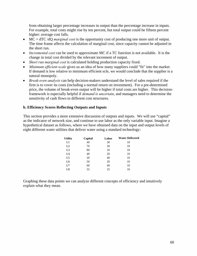
from obtaining larger percentage increases in output than the percentage increase in inputs. For example, total costs might rise by ten percent, but total output could be fifteen percent higher: average cost falls.

• MC = dTC /dQ marginal cost is the opportunity cost of producing one more unit of output. The time frame affects the calculation of marginal cost, since capacity cannot be adjusted in the short run.

• Incremental cost can be used to approximate MC if a TC function is not available. It is the change in total cost divided by the relevant increment of output.

• Short run marginal cost is calculated holding production capacity fixed. • Minimum efficient scale gives us an idea of how many suppliers could "fit" into the market.

If demand is low relative to minimum efficient scle, we would conclude that the supplier is a natural monopoly.

• Break-even analysis can help decision-makers understand the level of sales required if the firm is to cover its costs (including a normal return on investment). For a pre-determined price, the volume of break-even output will be higher if total costs are higher. This decision-framework is especially helpful if demand is uncertain, and managers need to determine the sensitivity of cash flows to different cost structures.

b. Efficiency Scores Reflecting Outputs and Inputs This section provides a more extensive discussion of outputs and inputs. We will use “capital” as the indicator of network size, and continue to use labor as the only variable input. Imagine a hypothetical dataset as follows, where we have obtained data on the input and output levels of eight different water utilities that deliver water using a standard technology:

Utility Water Delivered Capital Labor U1 40 30 10U2 70 30 10U3 80 10 10U4 40 20 10U5 20 40 10U6 50 20 10U7 60 40 10U8 55 25 10

Graphing these data points we can analyze different concepts of efficiency and intuitively explain what they mean.

60

Figure 11. Efficiency Frontier and Technical Efficiency

igure 11 shows how these eight firms will be compared against each other in terms of their

e

cing

to

he figure shows eight firms that produce the same amount of output by combining different gy

s l

fficiency Frontier: When this Efficiency Frontier is constructed by mathematical “closer” to

s,

U8

U2

U6

U7

U1

U3

U5

U4

0 20 40 60 80 100Capital

Labor 45

Efficiency Frontier

40

35

30A

B

25

20

15

10

5

0

Ftechnical efficiency levels. This means that each firm is going to be analyzed regarding how much output it is producing relative to the amount of inputs it is using, and considering that thtechnology available to all firms is exactly the same. The last condition implies a strong assumption that is presumed valid throughout the whole analysis. Then, if a firm is produmore output than another firm and it is utilizing the same amount of inputs in the process, the former can be labeled as technically more efficient than the latter. This technique will be able measure how much is the technical inefficiency of one firm with respect to others. Tamounts of labor and capital, which are the only two necessary inputs this production technolorequires. Since the firms are utilizing different combinations of both inputs, it seems difficult to compare how well they are performing in terms of technical efficiency. This task would be much easier if there were only one input utilized in the production process. However, what icalled an “Efficiency Frontier” can be constructed with the data points available. With that tooin hand, firms can be compared against each other even when they use a different combination oflabor and capital to produce the same amount of output. Eprogramming methods like the one used by DEA, a line connecting the points that arethe origin is found, in such a way that no point lies between the line and the origin. This line will probably have multiple kinks, and it should also slope downward, showing the substitution possibilities between the two inputs. This technique allows the analyst to compare all the firmby observing how far they are from the “frontier.” All the firms in the sample will be given a technical efficiency score even when there is probably no firm like her, in terms of using the same amount of capital (or network size), for example. If each firm had the same amount of

61

capital, then it would only remain to compare the amount of labor used, concluding that the firm using more capital is technically more inefficient than the other. In the specific example of Figure 11, the line is constructed connecting firms 3, 4, and 5. This means that only these three firms are able to determine the Efficiency Frontier in this case. By joining these 3 points, all the firms in the sample are categorized into two groups: on the frontier or away from it. The three firms used to construct it are obviously on the frontier and no technical inefficiency can be assigned to them. But the remaining firms outside the frontier are labeled as technically inefficient. They could reduce the amount of input/s used and still produce the same amount output than the firms on the frontier. For example, if firm 1 moved to point A, it could reduce both the amount of labor and the amount of capital utilized, and still produce the same level of output. The same is true for firm 6, which could move to point B by using a lower capital and lower labor combination of inputs to still produce its actual output level. Notice that in the conclusion about where a firm should move to be technically efficient, we indicate a “virtual” point on the frontier where probably no firm is now operating. We tell firm 1 to move to point A and we also tell firm 6 to use the labor capital combination depicted by point B, but we are aware that no firms are actually located at these points. This is a feature of the way the frontier is constructed. We presume that if a firm locates at A or B, it will be able to produce the same amount of output that firms 3, 4, and 5 are producing. After this intuitive explanation, we formalize how the technical efficiency score is constructed (Figure 12). We use firm 1 as an example. Since that firm could move to point A and still produce what it is now producing, the distance from the original point to A is somehow the “reduction” in inputs used that it should achieve in order to locate on the frontier. That distance reflects how “far” that firm is from the frontier. It then seems natural to compare that distance with respect to the distance between the origin and the point where the firm is now operating. This allows the analyst to quantify how important the first distance is: it is not the same to reduce one unit of labor and capital if the firm is now using 10 of each, than if the firm is now using 100 of each. Then, the technical efficiency definition concludes that the percentage found by dividing the two distances is the level of inefficiency that could be eliminated by using a different combination of labor and capital. In terms of firm 1 that is being used as the example, the distance from the origin to point U1 reflects how “big” the actual capital-labor combination is. And the distance from the origin to point A depicts how big it should be, according to the frontier just constructed. Then, the distance from A to U1 reflects the size of the “reduction” in inputs used to be attained if the firm wants to move to the frontier. Then, the technical efficiency score is defined as the ratio of the segments OA/OU1<1 (since OA<OU1). Similarly for firm 6, its technical efficiency score is denoted by OB/OU6<1. Notice that if we perform that calculation for firms 3, 4, and 5, we get an efficiency score of 1, since there is no input reduction available, and then the segments joining the origin with the

62

optimal and the actual input combinations are the same. For firm 3, for example, we have OU3/OU3=1.

Figure 12. Allocative Efficiency and Technical Efficiency

The same eight firms that were analyzed in terms of their technical efficiency levels will now be compared in terms of a different efficiency concept: allocative efficiency. This new efficiency concept focuses on how well the firm accounts for input prices in its production process. The technical efficiency concept only analyzed how much output the firm was able to produce from a given basket of inputs. It only focused on the technological point of view, reflecting an engineering approach, and ignoring input prices. This new efficiency concept is useful for evaluating the combination of inputs used, even when the firm may be technically efficient. That is, even when the firm may be satisfied with its technical efficiency score (because she cannot reduce inputs and still produce its actual output level), the allocative efficiency concept goes a step further. By incorporating input prices in the analysis, it can suggest a different input combination that keeps output constant but reduces the total expenditures of the firm. For example, we had suggested to firm 1 that it should move to point A in order to be technically efficient. By this change in its input combination the firm moved to the efficiency frontier and was able to get a score of 1 in terms of technical efficiency. But when the allocative efficiency concept is applied, it shows that the firm can do even better. To explain why this is the case, we need to introduce the isocost curve into the analysis. This straight, downward sloping line reflects all the possible capital labor combinations that can be achieved by spending the same, fixed amount of money on them. The slope of that line reflects the relative prices of inputs. By fixing total expenditures at some level, we can easily construct the line by joining two points. The first point will be on the horizontal axis, and it is found by dividing the total (fixed) expenditures by the price of capital (80 in our graph). The second point will be on the vertical axis, and it is found by dividing the total (fixed) expenditures by the price of labor (40 in our graph). As it is clear, those points tell us what is the maximum amount of one

U4

U5

U3

U1

U7

U6

U2U8

05

1015202530354045

0 20 40 60 80 100Capital

Labor

Efficiency Frontier

Isocost Line

A

B

C

D

63

of the inputs that can be purchased if the firm decides to spend all the money on just that input. Hence, the isocost line connecting these two points tells us how we can move from a point where the firm buys only labor to a point where the firm buys only capital, while keeping total expenditures constant. Points C, D and U4, for example, show us different combinations of labor and capital that can be purchased by using the same expenditure level. These points lie on the isocost line, as well as (80,0) and (0,40) as has been already mentioned. Changes of input prices will change the slope of the isocost line. For example, if capital was suddenly cheaper the firm could get more than 80 units of it without changing its total expenditures. On the other hand, a lower price of labor would allow the firm to get more than 40 units of it if spending all the money in labor. Changes in total expenditures, on the other hand, do not modify the slope of the line but they shift its position on the graph. A higher expenditure level allows the firm to get larger quantities of both inputs, hence moving the isocost line away from the origin. Once the isocost line is introduced, the allocative efficiency concept is easily explained. We said that if firm 1 moved from U1 to A, it eliminated all its technical inefficiency. And we also mentioned that the firm can go further and improve its performance even more, now in terms of the new allocative efficiency concept. The way the firm can do this is by moving along the efficiency frontier until she gets to the lowest possible isocost line. If firm 1 moves from A to U4, she is still being technically efficient since no movement away from the frontier has occurred. But the firm is being more efficient in terms of its allocation of resources, because it is reducing the total expenditures on inputs while keeping output at the same level. Then, a way to measure allocative efficiency is by comparing the cost actually incurred with the (presumably lower) cost that could be attained if utilizing a different input combination, while keeping output unchanged. This ideal cost is dictated by the isocost line. For example, a measure of allocative inefficiency for firm 1 is found when comparing the potential cost savings (segment CA) with respect to the actual cost (segment OA). The same reasoning applies if we want to find the allocative efficiency score for the same firm: it is given by the ratio of the segment OC (lowest possible cost for that level of output) and the segment OA (actual expenditure). Then, the ratio OC/OA<1 is the allocative efficiency score for firm 1. Similarly, the ratio OD/OB<1 is the allocative efficiency measure for firm 1. Now, if we pay attention to the performance of firm 4, we observe that there is no possible cost reduction while keeping output constant. There is no movement along the efficiency frontier that would allow it to spend less on inputs and at the same time produce the former level of output. Then, the conclusion is that firm 4 is allocatively efficient: its ratio is OU4/OU4=1. The separation of inefficiency into technical and allocative allows the introduction of a broader concept: total efficiency. We can keep utilizing firm 1 as an example, as follows. Firm 1 is producing at point U1. At that particular point we found a level of inefficiency given by the segment AU1 (potential input usage savings), and a level of allocative inefficiency given by the segment CA (potential expenditures savings). Intuitively, the combination of both inefficiencies accounts for the total inefficiency that firm 1 is experiencing. Formalizing this concept into efficiency scores, we have technical efficiency TE=OA/OU1 and allocative efficiency AE=OC/OA. The product of the two gives the total economic efficiency EE=OC/OU1, after the

64

simplification of OA in both numerator and denominator. For firm 6 for example, we have TE=OB/OU6 and AE=OD/OB, both composing a score of EE=OD/OU6. The same can be done for all the firms in the sample. A final word should be said regarding firm 4, which we already found as being technically efficient. Also notice that this firm faces no potential cost savings, since it is not away from the isocost line, as it was the case for all the other firms (even if on the frontier). Then, firm 4 can be labeled as the only economically efficient firm in the sample. It has a score of 1 in both the TE score, as well as the AE score. Also important to notice is that being economically efficient necessarily implies being also technically efficient. But the reverse is not true: even if you are technically efficient, you can still be economically inefficient because of a score less than 1 regarding allocative efficiency. c. Outputs and Costs This section further develops efficiency notions in the context of costs. After considering Scale efficiency, we will describe statistical techniques for estimating a linear cost relationship. Then, we will see that the data might support a more complicated functional relationship. Scale efficiency: For the final efficiency concept that will be introduced, scale efficiency, we base our graph on a new hypothetical dataset showing several firms producing different output levels at different operating costs:

Water DeliveredUtility Operating CostA 20 10B 40 20C 30 30D 50 40E 55 30F 60 50

Figure 13 shows this situation graphically, with output measured on the vertical axis and costs measured along the horizontal axis:

65

Figure 13. Scale Efficiency

60 Water Delivered

The scale efficiency concept is very important in the water industry, since firms are usually considered to face economies of scale, meaning that they could double the amount of output produced without doubling the cost of producing it. Then, it would be useful to measure if that is the case in any particular study of efficiency across water utilities. Again, we would like to find a frontier in order to compare the performance of each firm with the ideal one. The mathematical programming techniques used by DEA would construct such a frontier by finding a line that leaves all the utilities either on the frontier or below it. Then, a firm that ends up on the frontier is said to have no scale inefficiency, while a firm below the frontier is suffering from scale inefficiency. An important distinction has to be made regarding the way the frontier is constructed. If the analyst considers that the industry is characterized by constant returns to scale (CRS) (i.e., doubling output would imply doubling costs), then the frontier is constructed as a straight line joining the origin with the firm depicting the highest ratio water/cost. In Figure 4 that line is the red, straight line passing through point C. But if the analyst considers that the industry is characterized by variable returns to scale (VRS), a different frontier has to be constructed (the kinked one in the graph). This frontier still leaves many firms away from it, but there are some firms that look better now since they are now positioned on the frontier. Which of the two approaches is taken is a decision residing on the analyst, which should judge if reality is better explained in one way or the other. Of course, the scale efficiency score obtained for each particular firm will differ under both approaches (except for firm C, that is the one picked to construct the CRS frontier).

B

A

EC

F

D

0

10

20

30

40

50

0 10 20 30 40 50 60 70 OPEX

CRS Frontier

VRS Frontier

x x1x2

66

After having explained the two options regarding returns to scale, then measuring the scale efficiency score is similar to what we have explained before. Intuitively, it is just a ratio of two distances on the graph: what it should be over what it is. The score will be then less than 1 in case the firm has something to improve, but it will be equal to 1 in case the firm is doing exactly what it has to do. Utilizing firm B as an example, a scale efficiency analysis under the CRS assumption indicates an efficiency score of xx1/xB<1. This scale efficiency score less than 1 says that the firm is not operating efficiency according to the CRS assumption. According to the output level of 20 units produced, the firm should have a cost of 20 rather then the actual 40, as can be observed in the table above. On the contrary, given a VRS assumption, firm B faces a scale efficiency score of xx2/xB<1. This score less than one still indicates inefficiency for this utility, since costs are larger than what they should be for this output level. But the VRS assumption is more lenient, and suggests a cost reduction to only (around) 25 units from the actual 40. It is then really clear why the “returns to scale” assumption is so important. Under the CRS assumption, only firm C is labeled as being scale efficient, while under the VRS assumption, also firms A and F are considered as scale efficient. The more different is a firm to the one used to construct the CRS frontier (in terms of output level), the more severely punished it is by that assumption. d. Statistical Estimates of a Linear Cost Function The table below shows hypothetical data from a sample of 8 utilities. We assume we have collected data on cost and water delivered from all of them.

Utilities Water delivered Cost

A 3 18 B 3.5 20 C 4 10 D 5 27 E 6 36 F 7 53 G 8 33 H 9 62

Figure 14 is constructed from these data. It depicts cost on the vertical axis, and water delivered on the horizontal axis. It shows how three different cost frontiers would look like, depending on which statistical approach is taken to derive it: ordinary least squares (OLS), corrected ordinary least squares (COLS) and stochastic frontier analysis ( SFA).

67

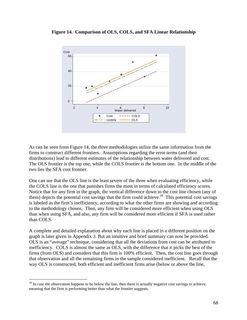
Figure 14. Comparison of OLS, COLS, and SFA Linear Relationship

Cost 60

40

20

0

4 2 6 8 10Water delivered

Cost COLScostsfa OLS

As can be seen from Figure 14, the three methodologies utilize the same information from the firms to construct different frontiers. Assumptions regarding the error terms (and their distributions) lead to different estimates of the relationship between water delivered and cost. The OLS frontier is the top one, while the COLS frontier is the bottom one. In the middle of the two lies the SFA cost frontier. One can see that the OLS line is the least severe of the three when evaluating efficiency, while the COLS line is the one that punishes firms the most in terms of calculated efficiency scores. Notice that for any firm in the graph, the vertical difference down to the cost line chosen (any of them) depicts the potential cost savings that the firm could achieve.18 This potential cost savings is labeled as the firm’s inefficiency, according to what the other firms are showing and according to the methodology chosen. Then, any firm will be considered more efficient when using OLS than when using SFA, and also, any firm will be considered more efficient if SFA is used rather than COLS. A complete and detailed explanation about why each line is placed in a different position on the graph is later given in Appendix 3. But an intuitive and brief summary can now be provided. OLS is an “average” technique, considering that all the deviations from cost can be attributed to inefficiency. COLS is almost the same as OLS, with the difference that it picks the best of the firms (from OLS) and considers that this firm is 100% efficient. Then, the cost line goes through that observation and all the remaining firms in the sample considered inefficient. Recall that the way OLS is constructed, both efficient and inefficient firms arise (below or above the line,

18 In case the observation happens to be below the line, then there is actually negative cost savings to achieve, meaning that the firm is performing better than what the frontier suggests.

68

respectively). This idea helps to explain why the COLS line punishes firms much more severely than OLS. Regarding SFA, it partially alleviates the severity of COLS and then situates as a compromising solution between OLS and COLS. It does so by still assuming that part of the deviation from cost is attributed to inefficiency (as COLS), but it also admits that part of that deviation can be considered just a random disturbance (i.e., statistical noise or measurement error). Then, SFA takes away part of the difference between real and estimated (ideal) cost, ending up with a smaller estimation of inefficiency. It assumes that the firm does not have to catch up all that deviation, but only some part of it in order to become 100% efficient. e. Specification of a Nonlinear Relationship Consider the same utilities used in the previous example but with two changes in reported costs: Utility F has total cost of 40 and Utility H has total cost of 45.

Utilities Water delivered cost

A 3 18 B 3.5 20 C 4 10 D 5 27 E 6 36 F 7 40 G 8 33 H 9 45

Figure 15 shows the new observations. Now, it appears that the linear relationship that would have been estimated using OLS, COLS, or SFA is no longer present. The relationship between production volume (water delivered) and total cost is now non-liner.

69

Figure 15. Possible Nonlinear Cost Function (due to changes in two observations)

From Figure 17, we can see that total cost still rises with increased volumes of water, but cost does not rise proportionately. Such a relationship would indicate economies of scale since the observations refer to utilities of different capacities. A more comprehensive discussion of different functional forms is left to the Technical Appendices. Suffice it to note, that model specification should take potential nonlinearities into account. IV. Strengths and Limitations of Different Methodologies: Technical Considerations

The objective of this section is to examine in greater detail the strengths and limitations of different methodologies and describe ways to determine the robustness of performance rankings. The Benchmarking Checklist summarized this material, but it is useful to have a more comprehensive basis for evaluating alternative methodologies. The preceding section provided the intuition behind several statistical approaches to modeling production and costs. This section goes into more detail regarding the strengths and limitations of the different methodologies: a. Criteria for Selecting Performance Measures Before considering the different methodologies that have been introduced through examples and graphs, we need to review the principal criteria for choosing a set of performance measures: they should be comprehensible, comprehensive, useable, and timely. • Comprehensible: The measures selected should allow for the production of the essential

information on the company’s overall performance. It is not very useful to have dozens of

0

20

40

60Cost

2 4 6 8Water delivered

70

measures if there is no framework for integrating them into a measure of overall performance.

• Comprehensive: A large number of productivity measures may provide a comprehensive

picture of a firm’s behavior but it is typically difficult to determine the accuracy of rankings or scores. Thus, the performance score is not readily comprehended and may create confusion if some indicators move in opposite directions. Comprehensive summary measures are needed.

• Useable: The intended audience must understand the indicators and how they are affected by

external developments (beyond the WSS utility’s control) or internal actions. • Timely: Poor performance in the past may have been already corrected, so having current

information is necessary to assess actual performance. We shall see that no single approach provides a comprehensive index of overall performance. However, one could argue that production and cost function studies have been underutilized by regulators and managers. b. Partial Indicators (Partial Metric Methods) Concept: The partial metric method consists of calculating different measures of the financial, operating, commercial, and quality firm’s specific factors. Performance indicators can be based on cross-sectional comparisons with competitors or comparable firms in other countries, while past performance can provide information on improvements over time. In general, these indicators account for the relationship of two simple measures, yielding indices of productivity, leakage and theft, human capital development, or financial conditions, among others. Such performance indicators include, for example, the number of workers per one thousand connections, the percentage of water loss, training outlays as a percentage of labor costs, or the ratio of total debt to total assets. When presenting the benchmarking results it is important to tailor the set of indicators to the purpose or to the intended audience. For instance, managers may view some of the indicators as not under their control. Hence, it is helpful to supplement the main indicators with summary measures to reinforce the effect of possible improvement actions. Within this group, we can identify Specific Core Indices, and Overall Performance Indicators (OPI). Specific Core Indices: A single index of utility performance has the same problems of any indicator: it will be neither comprehensive nor fully diagnostic. A physician can collect information on a patient’s temperature, pulse, height and weight. Those four indicators help the physician determine whether the person has a dangerous fever and/or is overweight. The indicators point to potential or existing health problems. A fever is a short term problem that can be addressed with specific medications; weight is a longer-term health issue with implications for the heart attacks and other problems—diet and exercise programs might be prescribed. However, a set of blood tests will provide more detailed information that can aid in diagnosing

71

the physical problems that are only partly reflected in the two health indicators. Similarly, diagnosing and treating mental health issues would require other diagnostics . . . and treatments. Nevertheless, Specific Core Indices (partial performance indicators) are widely used, and can serve as a starting point for evaluating performance. Examples of specific core indicators include the following: Quality of Service: these indicators measure how the company is delivering its service. Depending on the characteristics and the development of the water industry, some indicators are more relevant than others. For example, if the industry is well developed and every customer has access to water service during the day, the indicator continuity will not be as good an indicator of service as complaints per connection. Some quality indicators are: • Continuity (Hrs/day): number of hours per day (on average) of continuous water service. • Customers with minimum continuity (%): number of connections with continuity less than a

minimum established, divided by total number of connections (x 100). • Coverage (%): population served (number of connections multiplied by the number of

inhabitants per connection) divided by total population in the area. This measure may be disaggregated to consider type of connections, such as multi-family, single-family, industrial, commercial, or special purpose (e.g., hospitals and schools).

• Active Connections (%): number of connections delivering service divided by total number

of connections. A connection may not be active due to nonpayment or poor functioning. Consequently, this indicator may as well be a measure of the level of maintenance in the system.

• Complaints/1000 connections: number of complaints X 1000 divided by the number of

connections. Quality of Water: These indicators measure the physical quality of the water delivered. Depending on country standards, the presence of a certain percentage of chlorine is a good indicator as well as turbid or murky water level. Management Efficiency: These indicators measure how well management is controlling for factors that affect the production of service. For example, by applying a higher or lower level of maintenance to the system or by hiring more or fewer employees, the efficiency of the service may be affected. Some efficiency management indicators are the following: • Water not accounted for (%): The ratio of volume of water billed to volume of water

produced. This ratio captures physical losses (poor maintenance) and commercial losses (inefficient billing and illegal connections).

• Leaks (#/km): Ratio of number of leaks to length of network.

72

• Level of metering (%): Ratio of number of meters to number of connections (X100). If active connections are used, then meters should also be active.

• Percentage of customers with metering: Total number of connections with metering divided by total number of connections

• Percentage of water sold with metering: Total volume of water sold to customers with a

meter divided by total volume of water sold. • Water produced per inhabitant (m3/inh): Ratio of total volume produced to total population

served • Number of workers/1000 connections: Ratio of number of employees (direct and indirect) to

total number of connections (X1000). Financial Performance Ratios: A water service company that can remain in business, but has financial concerns will face recurring problems. Financial performance ratios such as unit operating cost, labor cost as a percentage of operating cost, and return on assets shed some light on possible areas of financial concern. More information on such ratios can be found in Appendix 1. Advantages of Specific Core Indices: These partial measures provide the simplest way to perform comparisons: performance indicators are easy to calculate, they seem easy to interpret, and the data are often readily available from annual reports of companies. Focus can be given to trends over time to create targets for utilities. Disadvantages of Specific Core Indices: Such indicators fail to account for the relationships among the different factors. A firm that performs well on one measure may do poorly on another, while one company doing reasonably well on all measures may not be viewed as the “most efficient” company. Application: Uganda’s National Water and Sewerage Corporation has used a few Specific Core Indicators (unaccounted for water, collections, and network expansion) to create strong incentives for managers of local water utilities. Performance contracts based on achieving these targets involve managerial bonuses of 50% of salary. Using simple trend information and comparisons across a set of utilities has had very positive impacts on NWSC performance.19 b. Aggregating Partial Indices into an Overall Performance Indicator (OPI) The specific core indices are often combined in some way to create an Overall Performance Indicator. The way this combination is usually performed is through a weighted average of core indices, where the weights reflect the importance the regulator assigns to each aspect of the firm performance. 19 Extracted from "Using Internal Incentive Contracts to Improve Water Utility Performance: The Case of Uganda’s NWSC," Silver Mugisha, Sanford V. Berg, William T. Muhairwe, May 2005 (forthcoming, Water Policy).

73

Advantages of Aggregating Partial Indices: The use of an OPI provides a summary index that can be used to communicate relative performance to a wide audience. Its components are easily understandable, providing some legitimacy to the resulting rankings. Disadvantages of Aggregating Partial Indices: The weights used to compute the OPI are generally not determined through a process that prioritizes different outcomes. Thus, when WSS are rated on the basis of a set of indicators, equal weight tends to be given to each component, even when the incremental costs of improving a particular ratio might be very high and the incremental benefits from the improved ratio minimal. Application: The regulator for the water sector in Peru, SUNASS, utilizes a set of specific core indices to assess the relative efficiency of the service companies. SUNASS has selected nine indicators, grouped in the following four areas of efficiency: 1. Quality of Service groups three variables: compliance with the residual chlorine rule, continuity of service, and percentage of water receiving chemical treatment. 2. Coverage of Service Attained groups two variables: water and sewerage coverage. 3. Management Efficiency groups three variables: operating efficiency (a combination of continuity of service and the volume of water produced to serve each person in a connection), percentage of connections with meter installed, and the ratio of bills not yet collected to the total number of bills. 4. Managerial Finance Efficiency is defined by the ratio of costs and expenses to revenues. The first two areas of efficiency are intended to represent the interests of society. The third reflects the companies' performance, and the fourth represents the stockholders' perspective. Each indicator was assigned a weight of 1 as a first step in the benchmarking process. The emphasis on social fairness is evident in the greater number of indicators related to efficiency affecting society. Each indicator expressed as a percentage is multiplied by its weight and added to the percentage total per company. This total per company is divided by nine, the number of indicators. Finally, each company providing water and sanitation services is ranked on the basis of points attained within a group, with groupings determined by number of service connections, as follows:

• 17 are small with fewer than 10,000 connections. • 20 are medium-sized, with 10,000–40,000 connections. • 7 are big, with 40,000–160,000 connections.

SEDAPAL, the water and sanitation utility of Lima, has about one million connections. A comprehensive performance comparison would treat this large utility separately, since its inclusion in the sample could distort the results. In Peru, each company sets its efficiency indicators within a master plan according to its financial and operational resources. This document is submitted annually to SUNASS for review

74

and approval. Once the master plan is approved, it is viewed as involving mandatory targets. At the end of the year, the ranking based on actual data is calculated by SUNASS and published. Similarly, the SEAWUN Benchmarking program in Asia develops an “Overall Performance Indicator” (OPI) based on the ten categories in the IBNet system: coverage, water consumption and production, unaccounted for water, metering practices, pipe network performance, costs and staffing, quality of service, billings and collections, financial performance, and capital investment. The OPI reflects relative performance on fourteen partial indictors. d. Performance Scores Based on Production and Cost Estimates (“Total” Methods) This methodology has been discussed in some detail already. But it is useful to introduce additional observations about these techniques. Total methods underline the interrelationship analysis of several inputs and outputs of a single firm allowing for the identification of distinct types of efficiency/inefficiency such as technical or cost efficiency. Total methods may be classified as Error! Reference source not found. Error! Reference source not found., Error! Reference source not found. Error! Reference source not found., or Error! Reference source not found. Error! Reference source not found., depending upon the primary intent of benchmarking, the type and quantity of data available, and the resources at the disposal for the needed calculations. As with performance indicators, cross sectional comparisons within industry or with other countries may complement or enrich the analysis. In particular, international benchmarking is used when there are not enough data, as in the case of a newly reformed sector or in the presence of a monopoly. Caution is necessary when making international comparisons to account for those factors that differentiate the analyzed countries, such as economic, political risk, and technological factors.

i. Index Methods (Total Factor Productivity) Concept: How much output is achieved with each unit of input? Total Factor Productivity is a measure of the physical output produced from the use of a given quantity of inputs by the firm. When having multiple outputs and multiple inputs, the ratio of the weighted sum of outputs with respect to the weighted sum of inputs is used to calculate the Total Factor Productivity Index. In general, the weights are the cost share for inputs and the revenue shares for the outputs. Prices or cost shares and revenue shares may change between two periods. There are two alternatives in dealing with this problem which implies different calculations: same weights may be used in both periods, or each period may use a different weight. The focus of the analysis should be the factor by which the input in one period could be decreased such that the firm could still produce the same output level of a comparing period. This is known as the Malmquist index. In this case, the choices for calculation are the use of the final period, initial period, or geometric mean of both periods as the reference point. The Malmquist index may be used either with parametric or nonparametric specifications, but is more generally associated with DEA. When data on input quantities are not available, an indirect TFP index may be used. We could deflate total revenue and total costs by a suitable price index to obtain a quantity index. Then, we could directly use deflated revenues over deflated costs. If the price index does not have the

75

same scope (e.g., the input price index is related to the economy in general and the output price index is related to the particular industry), the TFP index will be biased. A final note should be made about measuring the TFP index change for a group of firms: pair wise comparisons will not necessarily give the same ranking of firms. These indexes need to be adjusted using a more complex calculation technique. Advantages of Index Methods: The approach only requires data on two observations, such as two firms or two time periods. Disadvantages of Index Methods: TFP cannot be decomposed into the different types of efficiencies (i.e. technical, allocative and economic, as mentioned earlier). Application of Index methods: This method has been used in the USA telecommunications sector.

ii. Mean and Average Methods Section III provided graphical examples of “fitting” observations to a linear model. The basic statistical skills required for performing such tests are not substantial, but care must be taken about model specification and data availability. “Outliers” are observations that can unduly affect the estimated coefficients, and thus performance evaluations of specific WSS. There are basically two methods within this category: a) Ordinary Least Squares (OLS) and b) Corrected Ordinary Least Squares (COLS):

a. Ordinary Least Squares (OLS) Concept: OLS techniques can be used to perform benchmarking that relates individual firm performance relative to what would be expected: an estimate of an average production or cost function of a sample of firms. Average benchmarking methods may be used to compare firms with relatively similar costs or when there is a lack of sufficient data of comparable firms for the application of frontier methods. Basically, the method refers to the estimation of a regression functional form for costs or production using the OLS approach. Linear regression analysis seeks to derive a relationship between firm performance (in terms of output or total cost) and market conditions and characteristics of the production processes. Statistical analysis can isolate the impacts of specific conditions or levels of output—so the roles of multiple independent variables can be determined. Data from the firms being compared can then be used to arrive at expected dimensions of firm performance, given the variables characterizing each firm. The technique of regression analysis is defined by the following steps: 1) selecting both the cost (or output) measure and exogenous variables, 2) estimating a cost (or production) function for the industry, and 3) calculating the efficiency coefficient for each firm within the industry. Predicted versus actual output provides a measure of relative performance. The quality of these results can then be statistically evaluated to provide the policy-maker with a framework for evaluating firms.

b. Corrected Ordinary Least Squares (COLS)

76

Concept: A slightly different approach than OLS involves shifting the line towards the best performing company, which is called Corrected Least Squares methodology (COLS). In a general sense, COLS is merely a shifted average function. Two steps are needed, one to get the expected value of the error term and another to shift or to “center” the equation. When using OLS or COLS it is good practice to perform Quantile analysis. Quantile analysis helps to overcome the possible effect of outliers on the estimated mean allowing the analyst to detect the presence of performers on specific or extreme quantiles such as the lower (25%) or the upper (75%) quantiles. Advantages of Mean and Average methods: The statistical method reveals information about cost structures and distinguishes between different variables’ roles in affecting output. Disadvantages of Mean and Average methods: A large data set is necessary in order to obtain reliable results. The regression results are sensitive to functional form if the error term is not adequately interpreted, which can lead to widely varying conclusions depending on how the regression is initially set up. Application: The UK water regulator OFWAT applies mean and average methods to the operating costs (OPEX) and capital expenditures (CAPEX) of water utilities when determining the price caps every five years. OFWAT has developed an efficiency analysis relying on mean and average methods that is a key part of its price determination process. Literally, OFWAT argues that:20

“The price limits we set companies are based on demanding efficiency assumptions. This encourages companies which perform poorly to catch up with the more efficient ones. We make comparisons between companies, against each individual company's targets, and with other sectors. We ask them to improve if this is necessary. In a monopoly of this sort we rely on comparative competition. We give companies incentives to keep their running costs and the costs of maintaining their assets to the minimum necessary and to use cost-efficient solutions to achieve their outputs. Where companies are successful, they retain the savings for five years and customers benefit at the next price review through price limits which take account of the efficiencies achieved.”

iii. Frontier Methods

Concept: Frontier Benchmarking places a greater focus than average benchmarking on performance variations among companies. Frontier-based benchmarking methods estimate (stochastic) or identify (non-stochastic) the efficient performance frontier from best practice in an industry or a sample of firms. The efficient frontier is the benchmark against which the relative performance of firms is measured. Given a certain sample of firms, all companies should be able to operate at an optimal efficiency level which is determined by the efficient companies in the sample. These efficient companies are usually referred as the “peer firms” and

20 See http://www.ofwat.gov.uk/aptrix/ofwat/publish.nsf/Content/protecting_interests280905

77

determine the efficiency frontier. The companies that form the efficient frontier use minimum quantity of inputs to produce the same quantity of outputs. The distance to the efficiency frontier provides a measure for the efficiency. If a large data set is available, this approach may be suitable at the initial stages of regulatory reform when the most pressing objective is to reduce the performance gap within the industry. We now explain in detail both approaches: a) Stochastic Frontier Analysis, and b) Non-Stochastic Frontiers: Data Envelopment Analysis (DEA):

a) Stochastic Frontier Analysis Stochastic Frontier Analysis attempts to estimate an efficient frontier which does incorporates the possibility of measurement error or chance factors in its estimation. To separate inefficiency and noise, strong assumptions are needed on the distribution of noise among each observed firm. Stochastic frontiers may be classified as Production, Cost, and Input Distance frontiers. A production frontier reveals technical relationships between inputs and outputs of firms and represents an alternative when cost frontiers can not be calculated due to lack of data. The estimated output is the maximum possible output for given inputs of an individual firm. The output difference obtained in the estimation is interpreted as technical inefficiency of each individual firm. On a production frontier, variable returns to scale is the sensible option and appropriate scale efficiency changes need to be included when calculating total factor productivity. A cost frontier shows costs as a function of the level of output/s and the prices of inputs. It is useful when trying to access the wedge between tariff and minimum costs. Conceptually, the minimum cost function defines a frontier showing costs technically possible associated with various levels of inputs and control variables. Total cost frontier rather than variable or expenditure cost frontier is preferable to account for substitutability of factor inputs. Separate models for CAPEX and OPEX do not allow for allocation of expenditures between operating and capital expenditure. Cost efficiency contains the effects of technical and allocative efficiency. Each approach (production or cost) may yield different results. The difference will be larger if large allocative distortions are present. In this case, the parameters of the cost frontier will be biased. An important factor to consider when choosing between a cost frontier and a production frontier is that usually regulated firms are required to provide the service at a preset tariff and they must meet demand. In this sense, firms are not allowed to choose their own level of output which makes output an exogenous variable. The regulated firm maximizes benefits by minimizing its costs of producing a given level of output. Cost is the choice variable for the firm so a cost frontier approach is a more sensible choice. Finally, an input distance frontier is the natural option for regulated industries where output quantity is exogenous and input quantities are endogenous, and when the nature of the technology is multiple outputs or there is not data available on price of inputs. This is the case

78

for water and sewerage as different outputs under the same firm where their provision comes from shared inputs which jointly determine the production function. A distance function may have either an input or an output orientation. An input orientation looks at how much the input vector may be proportionally contracted with the output vector held fixed. An output orientation looks at how much the output vector may be proportionally expanded with the input vector held fixed. Input distance functions can be estimated by either stochastic or DEA methods. The advantage of a distance frontier with regard to a cost frontier is that firm is not assumed to be minimizing costs. With respect to production frontier is that it avoids the endogenous problem. Advantages of Stochastic Frontiers: Accounts for data noise such as data errors and omitted variables. Standard statistical tests can be used to test hypotheses on model specification and significance of the variables included on the model. It is also more amenable to modeling effects of other variables (e.g., environment, quality) Disadvantages of Stochastic Frontiers: There is a need of functional form and production technology specification. Also, the separation of noise and inefficiency relies on strong assumptions on the distribution of the error term Application: A number of studies utilize this technique. Appendix 2 lists some studies.

b) Non-Stochastic Frontiers: Data Envelopment Analysis (DEA) DEA is a method in which linear programming techniques are applied to a framework of a multi-input, multi-output production function. DEA benchmarks firms only against the best producers. The approach can be characterized as an extreme point method. The assumption is that if any one firm can produce a certain level of output utilizing a specific number of inputs, then any other firm of equal scale should be capable of doing the same. The most efficient producers for any given level form a “composite producer”, allowing an efficient solution for every level of input or output.21

Utilizing the selected variables such as unit cost and output, DEA searches for the points with the lowest unit cost for any given output, connecting those points to form the efficiency frontier. Any company not existing on the frontier is found to be inefficient. A numerical coefficient is given to each firm and it is defined by the ratio of the distance from the origin over its distance from the efficiency frontier. Advantages of DEA: It can easily accommodate a multiplicity of inputs and outputs, if the number of observations is adequate. Disadvantages of DEA: The results are sensitive to the selection of inputs and outputs, so their relative importance needs to be analyzed prior to the calculation. However, there is no way to test their appropriateness. The number of efficient firms on the frontier tends to increase with the number of inputs and output variables. When there is no relationship between explanatory 21 A useful website at Warwick University contains tutorials and examples on DEA: http://www.deazone.com/ .

79

factors (within inputs and/or within outputs), DEA views each company as unique and fully efficient and efficient scores are very close to 1, which results in a loss of discriminatory power of the method. Application: Regarding the electricity sector, the Norwegian authorities chose Data Envelope Analysis as their measuring tool to design an individualized regulatory rate for each firm based on their comparative efficiency. The input components included man-hours, losses, capital (lines and transformers only), and goods and services. The output variables were number of customers, energy delivered, length of lines, and degree of coastal exposure.

c. Examples of Empirical Studies There are far more quantitative analyses of electricity systems than water systems. For example, Jamasb and Pollitt (2001) survey a large number of studies examining scale economies and economies of scope for electricity suppliers. 22 We have noted that Graham Shuttleworth is very critical of studies that try to identify the relative performance of firms. Among other concerns, he argues that (for electric utilities):

“Our experience in Europe shows, however, that different versions of a DEA model will give quite different results and there is no way to tell which set of results is most reliable. Picking the “right” set of DEA scores then becomes just a matter of opinion, based on how inefficient one thinks (or would like to think) a company is.”

Such skepticism is not shared by all analysts, but Shuttleworth’s comments serve as a useful antidote to anyone who believes that running statistical regressions or DEA models will lead to easy answers regarding relative performance. Most of his concerns have been mentioned earlier, when explaining the reasons for not engaging in benchmarking. Clearly, robust rankings will require that several methodologies be utilized, and differences explained. If the same set of firms has relatively high scores (or low scores) regardless of methodology and over a range of reasonable model specifications, we can have some confidence that the procedures have identified strong (and weak) performers. Turning to water systems research, Table 8 presents an alphabetical listing of empirical studies of water systems: 22 Jamasb, T., Pollitt, M. (2001), “Benchmarking and regulation: International Electricity Experience. Utilites Policy 9 (3), 107-130.

80

Table 8. Empirical Studies of Water Systems

______________________________________________________________________________ Author Data Method Country/

Region Issues and questions

Ashton (2000) 10 firms from 1987-1997

Fixed effect-Cost function

U.K. Relative efficiency of the ten water utilities

Aubert and reynaud (2005)

211 firms from 1998 to 2000

SFA-Cost function (Translog)

U.S. / Wisconsin

Tests impacts of different regulatory schemes (e.g., price cap, rate of return, hybrid) on cost efficiency of water utilities.

Bhattacharyya et. al (1994)

225 public and 32 private water utilities in 1992

generalized variable cost function

U.S. Compares relative efficiency between public & private water utilities in U.S.

Bhattacharyya et. al (1995)

190 public and 31 private water utilities in 1992

SFA-Cost function (Translog)

U.S. Explores relative efficiency between private & public firms; impacts of number of emergency breakdowns, total distribution pipeline length, diversity in services on firm efficiency.

Berg and Lin (2005)

44 water utilities from 1996-1998

DEA, SFA-production function and SFA-distance function

Peru Evaluates consistency of water utility performance rankings (DEA, SFA, and SUNASS rankings).

Byrnes et. al (1986)

68 government-owned and 59 private water utilities in 1976

DEA U.S. Compares relative efficiency between public & private water utilities in U.S.

Clarke et. al (2004)

household surveys at city level

Summary statistics

Argentina, Bolivia, Brazil

Explores effects of privatization participation on coverage.

Corton (2003) 44 water utilities in 1998

OLS-Cost function

Peru Evaluates relative performance for Peruvian water utilities.

Cubbin (2005) Survey of efficiency studies

England, Wales, Scotland

Considers efficiency measurement in the water industry in England, Wales, Scotland.

Cubbin and Tzanidakis (1998)

29 water utilities in year 1994

OLS and DEA U.K. Compares ranking based on DEA and OLS.

Estache and Kouassi (2002)

21 water utilities from 1995-1997

Fixed Effect-Cost function

Africa Evaluates relative efficiency of African water utilities; potential impacts of institutional factors like corruption, governance, privatization on firm efficiency.

Estache and Rossi (1999)

50 water utilities in year 1995

SFA-Cost function

Asia and Pacific region

Compares result of SFA to those based on partial indicators; stresses the importance of using frontier methods.

81

Estache and Rossi (2002)

50 water companies in year 1995

SFA-Cost function

Asia and Pacific region

Compares relative efficiency between public & private water utilities in Asia and Pacific region.

Estache and Trujillo (2003)

4 provinces 1992-2001(unbalanced panel)

TFP Argentina Tests impact of 1990s reforms; shows that ignoring multi-production nature of operators (water & sewerage) leads to misleading policies on performance of operators.

Fabbri and Fraquelli (2003)

173 utilities in 1991 hedonic cost function

Italy Tests whether and how environmental & qualitative variables affect production process in Italian water industry.

Feigenbaum and Teeples (1983)

57 private and 262 government-owned utilies

hedonic cost function

U.S. Uses hedonic cost function to determine water service quality; estimation results indicate hedonic index of output yields significant improvement in explaining utility cost variation over scalar specifications of output.

Fox and Hofler (1986)

176 firms for 1981 SFA - Cost function

United States

Separation of production & distribution of water.

Efficiency of private vs. public firms.

Garcia and Thomas (2001)

55 firms in 1995-97 GMM - Cost function

France

Losses considered as an output to capture link with water sold; economies of scope between them: is it cheaper to produce more water than fix leaks with increased demand?

Hunt and Lynk (1995)

1980-88 OLS - Cost function

England and Wales

Separation of production & regulatory functions of Regional Water Authorities.

Economies of scope between both activities: lost after privatization?

Kim (1987) 60 firms for 1973 SFA - Cost function

United States

Economies of scale for multi-product water utilities: serving residential & nonresidential users.

Kirkpatrick et. al (2004)

110 firms for 2000 Statistics Africa Efficiency of private vs. public firms in low income economies.

DEA Different results from different methodologies.

SFA Institutional issues regarding privatization of water provision.

Lin (2005) 44 firms for 1996-01 SFA Peru Role of four different quality measures: environmental variables affecting technology, or output variables affecting level of efficiency.

Saal and Parker (2000)

1985-99 SFA - Cost function

England and Wales

Efficiency in terms of production costs after privatization.

82

Efficiency after regulatory tightening in terms of price-cap imposition.

Existence of economies of scale & economies of scope in the industry.

Saal and Parker (2001)

1985-99 TFP England and Wales

Performance improvement after privatization, at industry or company levels.

Increases in profitability resulting from RPI+K regulation attributed to improvements in their TFP.

Regulatory adjustment of price cap in 1995 led to changes in performance at industry & firm levels.

Saal, Parker and W. Jones (2004)

1985-2000 Input Distance functions

England and Wales

Productivity growth considering privatization & price cap imposition in period under analysis.

SFA Breakdown of productivity growth into technical, efficiency, & scale changes.

Saal and Parker (2005)

1985-2000 Input Distance functions

England and Wales

Separation of water & sewerage services with possible cost interactions.

SFA Do water & sewerage companies share same frontier with water-only companies?

Saal and Reid (2004)

1993-2003 SFA - Cost function

England and Wales

Evaluation of mandated investments in drinking water & sewerage treatment quality.

Effect of drinking water & environmental quality standards on the OPEX productivity growth rates.

Bias in estimation of productivity growth of hypothetical average firm if characteristics change over time.

Sabbioni (2005) 280 firms for 2002 SFA - Cost function

Brazil Comparison of ranking of firms according to stochastic cost frontier utilizing 3 alternative outputs & conditioning variables.

Teeples and Glyer (1987)

119 firms for 1980 OLS - Cost function

United States

Efficiency-ownership relationship estimation.

Thanassoulis (2000)

32 firms for 1992/3 DEA England and Wales

Uses DEA to estimate potential cost savings after 1994 price review.

OLS Complementarities of DEA & OLS when estimating comparative relative efficiency.

Thanassoulis (2000)

32 firms for 1992/3 DEA England and Wales

Estimation of potential cost savings in the distribution of water utilizing DEA; comparison of econometric estimates by

83

OFWAT.

Tupper and Resende (2004)

20 firms for 1996-00 DEA Brazil Complementarities between DEA and econometrics if accounting for water losses & network density.

OLS Potential cost savings & creation of reimbursement rule as yardstick.

Wallsten and Kosec (2005)

53245 firms for 1997-2003

Negative binomial

United States

Efficiency of private & public firms.

Which types of rules are private & public firms more likely to violate.

The listing illustrates the scope of these studies. These empirical studies are briefly summarized in Appendix 2: Annotated Bibliography of Benchmarking Studies. As one can see from the publication dates, there has been significant activity in benchmarking in recent years. Consistent data covering a number of years and firms are becoming available for a number of nations. However, most of the research has been academic in nature, or has involved external consulting contracts. Transferring requisite technical skills to regulatory commissions and companies will be essential if such comparisons are going to influence incentives in the future.

iv. Model Specification and Interpretation

Linear Relationship: Although the Regulator, policy-makers or even the firm’s managers know that there is a positive relationship between input factor quantities and output, the precise form of this functional relationship is not known with certainty. Let us assume that there is only one input. A suggested, somewhat simplistic mathematical relationship may be expressed as XY βα +=

Where Y represents output, such as water produced (also called dependent variable—on the left hand side of the equal sign); X is number of workers needed in the production process (also called explanatory variable or regressor--on the right hand side of the equal sign). The α and the β variables are called parameters and are estimated using the observations. One way to understand this equation is that a number of workers (X) are utilized to produce a certain volume of water (Y). This equation, which states that water produced is linearly related to labor, is an example of a mathematical model. This model assumes that there is an exact or deterministic relationship between water produced and labor. However, relationships among economic variables are generally inexact. If we were to obtain data on 500 service companies and plot a graph with number of workers in one axis and volume produced in the other axis we will find out that the 500 observations would not lie on a straight line. This is because in addition to number of workers, there are other variables missing, which also affect the production of water: other input factors to the production process which may be controlled by the firm, or other aspects particular to the firm environment but not under the control of the firm (such as climate and topography).

84

The presence of measurement errors occurred during the data collection process or other inaccuracies constitutes a random or stochastic component to be considered. Modeling Steps: The first step in a model specification process involves determining what are the firm’s outputs and inputs (some of which are not under the control of the manager). This specification entails the definition of the variable units: examples are liters per customer, number of workers, and total costs. As a natural step after definition, checking for data availability is essential. Then we need to make a decision on how to represent the technology (how inputs are transformed into outputs). This implies the selection of either a cost or a production approach. e. Model Selection and Data Availability: A cost function approach is based on output and input prices. A production function requires input quantities. Depending on the main intent of the analysis (either a cost or a production focus), and on the data availability, the exact determination of the functional forming needed (in our initial example it was linear). After selecting the model, the following task is to proceed to estimate the parameters. When we consider a stochastic term present in the model, we say that we “estimate” instead of “calculate” the parameters meaning that the value of the parameters estimated implicitly have a certain degree of error. Parameter estimates give empirical content to economic theory. Verification, or statistical inference: The estimation and verification are steps that go beyond the scope of this appendix. In any case, as a main advice, the process of model specification, as simple as it may look, need to be performed by a professional. Those performing benchmarking comparisons must avoid both miscalculation and misinterpretation. Next, we develop a more detailed explanation regarding the different model specifications commonly used in the water sector. Production vs. Cost Function: Because one of the main interests in analyzing the water sector from a benchmarking point of view is cost efficiency, a Cost Function specification has been more generally used. A Production Function relating output to input factors have been mostly employed to analyze technology efficiency, possible shifts of the technology, allocative efficiencies and scale economies. More recently, the awareness of the multi-output characteristic of the firm’s water production process on several countries have led to the use of Distance Function specification. The selection of a Cost, a Production or a Distance function depends on particular circumstances regarding five areas (Sabbioni 2005): a) Operating Environment: Assuming that the firm is minimizing costs (or, maximizing

profits), a production function or a distance function may be a natural option. If instead the firm has an “obligation” to service, as when it is required to supply full demand, a cost function may be more suitable.

b) Possible Endogeneity: It is been argued that input factors in a production function are jointly

determined with the output produced. This leads to an econometric issue called endogeneity which may produce inconsistent and biased parameters estimates. Obviously, this issue may be addressed using certain econometric tools; however, the estimation procedure becomes

85

more complicated when not enough variables are available. Cost or distance function specifications do not present this problem.

c) Data Limitations: The main issue when using a cost function is the availability of prices of

inputs, in particular the price (cost) of capital. Variables such as cost of energy, and labor are scarcely reported by firms. This limit the use of a cost function approach favoring either a production or a distance function.

d) Output definition: From a production process point of view, a firm may produce more than

one marketable product as it has been recognized recently in the water sector. Econometric analysis using a production function will entail the specification of several equations, which makes the estimation process more complex. When having multiple outputs the choice reduces to either cost or distance functions. DEA can also be utilized.

e) Technology specification: It is well known that factors other than input quantities may have

an effect on the production process: just to mention the most common, factors such as the economy, topology of the location, age of the network, or even company ownership have implications on the production process. There are two ways to introduce these factors into a production function model so far, by means of assuming that they directly affect the production process(technology) or by considering them as part of the possible inefficiency of the firm during its production process. Introducing these variables into a cost function specification requires more care since it may not be clear how they affect the cost process directly. Thus, carefully addressing these variables with respect to cost or quantities is necessary before stating the model specification for a cost approach.

Data Availability: Although a cost function model is the preferred choice when analyzing cost efficiency, the use of total cost or variable cost functions is also framed by availability of data. When assuming the stock of capital as fixed, meaning that elements of the firm’s machinery or equipment are not easily altered in a certain time period, the use of a Variable Cost specification is indicated and stock of capital enters as explanatory variable in the a variable cost function. This is a sensible assumption for the water sector where assets have very long service lives. Implicitly, it underlines that companies do not have influence over fixed factors such as capital. However, the likelihood of substantial input factor substitution among capital and other input factors, in particular labor, may suggest that a Total Cost function model is more appropriate. Yet, the limitation here, as it has already pointed out, is data availability.

Functional Form: Either for a Cost, Distance or Production approach, the functional form requires careful attention. We have seen how linear and non-linear relationships might be captured in an empirical analysis. Appendix 1 provides definitions of variables that have been used in benchmarking studies:

• Output Variables • Quality Variables • Input Variables: Quantities and Prices • Accounting/Financial Variables

86

• Conditioning/Environmental Variables • Macroeconomic Variables • Governance Structure Variables

Appendix 2 contains an Annotated Bibliography of Water Benchmarking Studies. The reader can see the wide range of questions being asked: extent of scale economies, degree of economies of scope between water and sewerage production, and the relative efficiency of different water utilities, to note just a few. As noted earlier, the analyst should utilize several methodologies and specifications to test for the sensitivity of results to the number of years, the cross-section sample, variables, and model specification. Data availability and the issue under investigation will affect model specification. Statistical tests described in Appendix 3 can be used to determine which functional form is most appropriate. d. Other Methodologies

Three other methodologies have been discussed in some detail. The Engineering/Model Company approach has been used to establish baseline performance expectations. The use of an “artificial” firm that has optimized its network design and minimizes its operating costs can provide insight into what is possible if a firm is starting as a Greenfield Project. As with the metric methodologies described above, the approach also has its limitations. A second methodology focuses on individual production processes: Process Benchmarking. One advantage of this approach is the ability to identify specific stages of the production process that warrant attention to improve WSS performance. A third methodology, Customer Survey Benchmarking, focuses on the perceptions of customers as a key element for performance evaluation. Like the other approaches, this technique can shed light on consumer concerns, reflected in complaints or in customer surveys. We now turn to a more detailed explanation about the three approaches: Error! Reference source not found. Error! Reference source not found., Error! Reference source not found. Error! Reference source not found., and Error! Reference source not found. Error! Reference source not found.:

i. Engineering (Model Company) Approach A technique of comparative performance analysis noted here could be viewed as an extension of the metric method, generally referred as the “model company” method. This is an optimized economic and engineering model and differs from the earlier approaches because it is based on an idealized benchmark specific to each regulated industry—including the topology and density of the service territory, and not a cross-comparison of similar companies. This method consists of defining the needs of an industry in order to design a benchmark that most adequately reflects the optimal way in which to satisfy predicted demand. The model company approach combines both engineering efficiency (an analysis of the physical configuration of the network components of an industry) and economic efficiency (the application of least-cost functions to determine optimal operating costs) to design an optimized model of the firm or industry.

87

Advantage of the Engineering approach: Engineering models are not dependent on obtaining and analyzing the data of “real” companies. This point is important for two reasons. First, the use of the “model company approach” avoids the problem of insufficient data by which to measure a company’s efficiency. Secondly, it avoids categorizing a specific company as the ideal when it is inevitable that it would itself display some level of inefficiency, either due to capital wear and tear or managerial short-comings. This method identifies an optimal level of efficiency by which a company can be compared, thereby avoiding the problems that arise in a yardstick measure based on the similarity of companies and their production data. Disadvantage of the Engineering approach: The engineering models that support such an approach can be very complicated, and the structure of the underlying production relationships can be obscured through a set of assumed coefficients used in the optimization process. Application: The Chilean water sector utilizes this approach. In that particular case, it is called “Empresa Modelo” (Model Company) approach.23 It consists of defining the firm and designing the efficient investments to satisfy the forecasted demand. Investments are then valued at what it would cost to make them. The Chilean regulator argues that the application of this method into the sanitation sector is relatively simple, because:

All the production stages are regulated. There are usually no “multi-product” investments for serving unregulated markets. The main cost component is the return on capital and the depreciation of assets Inputs are purchased in competitive markets. There are not sudden and unexpected technological changes.

Using this method, the regulator abstracts from the inefficiencies of the real firms, and designs a theoretical company that is technically and economically efficient. Of course, being theoretical does not mean being unreal, since the model should allow the firm to meet forecast demand, and required quality standards and constrained by the available technology, and geographic and demographic features. The main concern in Chile resides on how to correctly address the “updating” that this model implies. The methodology assumes that there is a new firm being designed every time the analysis is done, and that may not adequately reflect former investments in assets that may have been done prudently and according to a reasonable scenario foreseen at the time that decision was made.

ii. Process Benchmarking Many organizations have started working with Process Benchmarking since the framework fits nicely into an operational approach to improving performance.

23 This is extracted from Morande F. and Doña Ilades, J. “Los servicios de agua potable en Chile: Condicionantes, institucionalidad y aspectos de Economia Politica”, Interamerican Development Bank, Documento de Trabajo R-308, 1997. We also thank Magali Espinosa Sarria from SISS (Chile), for her clarifications on this issue.

88

Concept:24 Process Benchmarking focuses on selected production processes in the business rather than on the business as a whole. The presumption behind the analysis is that by identifying best practice processes and comparing actual processes that firms utilize, managers can improve the performance of sub-systems—leading to better overall performance. The goal of process benchmarking is to improve different stages of the production process and to increase efficiency by “learning from others”. Sharing experiences is crucial for the success of the technique. For example, by comparing specific core indicators (and the procedures currently used that affect those indicators) for a set of utilities, best practice can be hopefully identified and transferred to weak performers, who should adopt in order to increase efficiency. Thus, Process benchmarking consists of a mechanism for identifying specific work procedures that could be improved by imitating external examples of excellence that can be set as the best standard in the industry. In that sense, Process Benchmarking involves the comparison of one’s own utility with other similar utilities, with the purpose of self-improvement through adopting structures or methods that happen to be successful elsewhere. Summarizing, it allows a firm to find out how others do business, whether they are more efficient or not and, if so, whether the firm can understand and use those methods to its own advantage. Recall that metric benchmarking identifies areas of weak performance where changes need to be made to the way things are done, while process benchmarking is a vehicle for achieving this change. According to Process Benchmarking, the improvement required could be imported from other best practice partners. Advantages of Process Benchmarking: Such detailed benchmarking includes comparisons of engineering practices, data collection procedures, office routines and performance indicators for each of the processes under study. Flow diagrams can capture key relationships and assist managers in identifying areas for improvement. Disadvantages of Process Benchmarking: The focus on specific procedures is very management-oriented, which means that an external monitor must depend on the information provided by utilities. Comparisons across utilities can be problematic due to idiosyncratic issues. Application: The Netherlands Waterworks Association (Vewin) and the Scandinavian Six Cities Group (composed of Copenhagen, Helsinki, Oslo, Stockholm, Gothenburg and Malmö) have used process benchmarking to identify and isolate areas for improvement. In the first case, for example, the benchmarking exercise is based on the most commonly used work processes in the water industry:

Production Distribution Sales General processes

The meaning and what activities the four processes include is as follows:25

24 Extracted mainly from Mats Larsson, Renato Parena, Ed Smeets and Ingrid Troquet, (2002)“Process Benchmarking in the Water Industry: Towards a Worldwide Approach”, International Water Association. 25 Quoted from Larsson et.al (2002).

89

“Production Process: This comprises all activities relating to the pumping up, intake, transport, clarification and filtration of groundwater as well as the purification and treatment of raw surface water by the production installations to obtained finished drinking water. It involves:

Designing Production Facilities Coordinating siting Operating Production Facilities Maintaining Production Facilities

Distribution Process: This stage includes all activities aimed at guaranteeing an uninterrupted supply to consumers of sufficient quantities of drinking water of a good and consistent quality, such as the maintenance of finished-water transport lines, mains and feeders. It involves:

Designing Pipeline Networks Building Pipeline Networks Maintaining mains Pipelines Placing and Maintaining Feeders

Sales Processes: This stage comprises all service activities focused on the company’s relationships with drinking water consumers. These activities mainly relate to meter reading and data processing, drinking water supplier or services rendered invoicing, debtor management and debt collection. It also includes handling of customers’ queries, requests and complaints. A detailed list would include:

Meter reading and processing of water consumption data Invoicing, debtor management, debt collection Maintaining customer relations

General Processes: This stage relates to the management of water collection and water protection areas and water quality monitoring on the one hand, and support activities on the other. Support activities relate to strategic policy development, marketing and public relations, personnel management, finance and economics, purchasing, etc. The specific processes here involved are:

Managing Water Collection and Water Protection Areas Monitoring Water Quality Planning Process Developing Strategic Policy Carrying out marketing and PR activities Recruiting and Managing Personnel Managing financial/economic affairs Information Technology and computerization Purchasing and warehouse management Facility Services”

90

iii. Customer Service Benchmarking Concept: Customer perceptions regarding service quality are central to evaluating water utility performance. Parasuraman et. al. (1985)26 developed the SERVQUAL model, identifying five dimensions of service quality as perceived by customers:

External Characteristics or Tangibles (tidy workplace, employee appearances) Reliability (meeting deadlines, consistency in interactions) Responsiveness (providing service promptly) Consideration or Assurance (personnel who are courteous, friendly, and polite: trustful

and helpful). Empathy (giving individual care and attention: comprehensible transactions)

Documenting performance on these dimensions can lead to changes in procedures that affect customer attitudes. SERVQUAL is then an empirically derived method that may be used by a services organization to improve service quality. The method involves the development of an understanding of the perceived service needs of target customers. These measured perceptions of service quality for the organization in question are then compared to an organization that is “excellent”. The resulting gap analysis may then be used as a driver for service quality improvement. Advantages of Customer Service Benchmarking: Surveys can reveal performance gaps and identify areas of concern. Customer complaints provide a direct indicator of consumer perceptions. Disaggregating complaints by type of customer, location, and type of complaint can help managers identify problem areas. In addition, trends over time can be used by regulators and policy-makers to evaluate utility performance. Disadvantages of Customer Service Benchmarking: Many other factors are relevant for the efficient provision of water services. Citizens not receiving service are not likely to be surveyed. Also, the use of difference scores in calculating SERVQUAL contributes to problems with the reliability, discriminant validity, convergent validity and predictive validity of the measurement. Hence, caution should be exercised in the use of SERVQUAL scores. Finally, SERQUAL assumes that the results of market surveys are accurate, and it also assumes that customer needs can be documented and captured, and that they remain stable during the whole process. Application: Many water utilities use surveys to determine customer attitudes and concerns. Regulatory commissions examine lists of complaints to identify areas in need of improvement.

26 Parasuraman, Zeithaml and Berry (1985) “A Conceptual Model of Service Quality and its implications for future research,” Journal of Marketing 49 (4), Fall, 41-50. Also see, R. Parena (1999). The IWSA Benchmarking Initiatives: Performance Indicators for Water and Sewage Services—An Actual Tool for Better Management and Public Regulation. Hydrocontrol International Workshop, Cagliari, Italy.

91

V. Summary and Conclusions

This Survey provides complementary material that complements Toolkits and other resources becoming available to those implementing public policy.27 The purpose is to help decision-makers become more effective producers and consumers of benchmarking studies. While benchmarking is not a panacea for overcoming impediments to public and private investment, it does provide key inputs into public policy debates and managerial evaluations, with wide-ranging implications for the following:

(1) Sustainability of capital inflows, public deficits, and reform initiatives;28

(2) Poverty reduction and public perceptions regarding infrastructure reforms;29

(3) Development and implementation of incentives for improving WSS service performance;30 and (4) Appropriate roles for multinational organizations, donor nations, and regional cooperation in the provision of WSS services.

This Survey of Benchmarking Methodologies represents a natural step in making resource materials available to those engaged in reforming, regulating, and managing water and sewerage service utilities. To date, data specification, collection, and collation has been the focus of benchmarking programs.31 With several years of consistent data available for many utilities, the issue becomes one of how to utilize the data (including core indicators) in evaluating utility performance. A substantial body of technical literature exists, but an accessible overview of benchmarking methodologies is needed to help practitioners begin comprehensive analyses of those data.32

27 Benchmarking Water and Sanitation Utilities: A Start-Up Kit. May 1999. World Bank. Washington, DC. 28 Typically, investors seek government guarantees, but guarantees can blunt incentives to select efficient projects. In addition, guarantees can become liabilities affecting government budgets. For an overview of public and private initiatives, see William Easterly and Luis Serven (2003), The Limits of Stabilization: Infrastructure, Public Deficits and Growth in Latin America, World Bank, xv-208. 29 Water Governance for Poverty Reduction: Key Issues and the UNDP Response to Millennium Development Goals (2004), United Nations Development Programme, 1-93. 30 Mehta Meera (2003), Meeting the Financing Challenge for Water Supply and Sanitation: Incentives to Promote Reforms, Leverage Resources, and Improve Targeting, World Bank, May, 1-136. 31 “Review of the water supply and sanitation sector benchmarking practices and models in the EU and other regions”, Report for 6th EU Framework Programme for Research and Technological Development. March 1, 2004. 32 The World Bank Institute has published a technical volume that serves as a good starting point. See Coelli et. al. (2003), A Primer on Efficiency Measurement for Utilities and Transport Regulators (WBI Development Studies), xii-134.

92

This Survey is designed to highlight the strengths and limitations of alternative methodologies, without becoming excessively technical. Appendices provide additional resource material: an Annotated Bibliography, Technical Descriptions of the Methodologies, and Surveys of Benchmarking Activity in different regions of the world. Past benchmarking surveys have focused on Core Indices and Summary Indicators rather than the models and methodologies associated with production and cost functions. a. Audiences for Studies There are at least six audiences for yardstick comparisons: benchmarking specialists, the press, the general public, regulators, national and international policymakers, and utility managers. Benchmarking specialists produce and critique studies that utilize various methodologies. Rankings can be manipulated by choice of variables, model specification, sample size, time frame, and treatment of outliers. Because the stakes are high, affected parties have an interest in the relative and absolute performance evaluations prepared by analysts, and studies can be controversial. The press filters and highlights reports, using executive summaries and interviews. Although technical reports are not amenable to sound bites, most newspaper and television journalists seek the clear message that emerges from a benchmarking study. However, some seek sensational factoids that support their own ideological predilections and some lack the expertise to interpret technical studies. The general public is not well-positioned to evaluate conflicting claims. Long before a benchmark comparison is released, the responsible agency should be engaging in an information-dissemination campaign, informing political leaders and the press about the purpose of the forthcoming report. NGOs and formal citizen advisory committees that can be established by regulatory commissions provide opportunities for input and feedback for citizens. The regulator reviews studies and creates performance incentives to achieve policy objectives. Productivity measures and other measures of technical efficiency provide valuable information for regulators. However, excessive simplicity can result in a distorted analysis. Sector performance also depends on efficient price signals, benefits from quality improvements, incorporation of environmental impacts into decisions, recognition of transition costs, and ability to meet agreed-upon social obligations. National policymakers (elected representatives and appointed officials) react to and utilize technical studies in setting priorities and interacting with international organizations. Solid data regarding the actual performance of public and privately owned utilities can be used to counter the politicization of infrastructure pricing. Water utility managers are sensitive to comparisons as they have much to lose (and something to gain) when information is made public. It is extremely difficult for outsiders to evaluate managerial performance. Inadequate reports and the selective presentation of information mean that only insiders know whether the organization is managed well or poorly. Benchmarking reduces the extent of this information asymmetry. For this reason, utility managers might delay or block serious benchmarking initiatives. b. Beginning the Benchmarking Process

93

Since efficiency evaluation plays such an important role in incentive regulation, regulators should be careful of the ranking techniques adopted from among parametric and non-parametric evaluation models. First of all, regulators should figure out what they really want to compare. They might want to focus only on cost minimization In this case, they can choose from among the regression model, COLS (corrected ordinary least square), SFA production (cost) function model or single output DEA models. If regulators want to measure other outputs simultaneously, such quality of service, they can choose to use a synthetic evaluation system (like SUNASS), DEA models or SFA input (output) distance function models. In addition, they would need to control for different conditions facing the utilities, such as customer density. There is some evidence of consistency of the efficiency measurement within specific groups of models, such as single or multiple output groups, but studies need to check this out. Second, regulators should be aware of the advantages and shortages of different models and choose the most appropriate ones to do the benchmarking and evaluation. In the case of Overall Performance Indicators (OPIs) as used by SUNASS and SEAWUN, the components are generally assigned equal weights. This weighting is arbitrary and not convincing. Regression models focus on the cost efficiency of a company, but can fail to consider other important factors such as quality of service, coverage of service, and financial sustainability of current prices. Nor does OLS consider the effect of the random shock or statistical noise. In addition, an inherent problem of regression analysis is that it requires specification of functional form, which risks fitting in an inappropriate function. Furthermore, regression analysis is limited to only one dependent variable, which might not depict the real world in a sophisticated way. DEA models do not have these limitations. DEA does not require the specification of a functional form to be fitted, nor does it need to impose weight to the factors. DEA allows for multiple outputs and inputs. In addition, DEA analysis can give us more information than the ranking. It can also be used to evaluate the return to scale and can set the goal for inefficient companies regarding how much they should improve to get on the efficient frontier. However, DEA models are not perfect either. The outcome of DEA analysis is sensitive to the selection of the models and different DEA methods. And DEA has been developed in a non-statistical framework, so hypothesis testing is problematic In addition, DEA does not account for possible noise. SFA is arguably a better method. It accounts for the effect of the random shocks and statistical noise and can accommodate multiple inputs and outputs by using the distance function. However, it also has potential problems; in particular, the standard SFA method uses a specific assumption on the residual skewness to separate inefficiency from measurement errors. There are still other techniques available, such as TFA (thick frontier approach) and DFA (distribution-free approach) (Berger 1991, 1993). All have their advantages and disadvantages. Third, regulators can select two to three appropriate techniques to construct models, conducting a three-level consistency tests to compare the outcomes of different methods and decide whether the model chosen is needed or not. If it is a panel data, regulators should also check whether these efficiency measures are consistent over time. If the consistency tests are satisfied, the regulator can choose one of the techniques arbitrarily. If the tests are not satisfied, extra emphasis should be put on the companies with coincident ranking and with totally opposite

94

rankings. In these ways, regulators can provide a relatively fair and convincing ranking to inform the public. c. Concluding Observations Benchmarking studies should target specific audiences with appropriate levels of detail. Each of the five benchmarking approaches can provide insights on aspects of water utility performance. Overall Performance Indicators combine partial metrics and provide information time trends and patterns across firms. This Survey focused on Performance Scores based on Production or Cost Estimates (“total” methods); these techniques can utilize the data sets that are becoming more widely available. Regional and international initiatives have been consolidated under the auspices of IBNet—leading to comparable data over time and across a large number of water utilities. Even prior to IBNet, research on production and cost functions grew at a rapid pace: we have identified thirty-five empirical studies of water utilities, and new studies appear each year. Techniques that are being applied vary in terms of technical skills required and ease of interpretation, but all can provide important information for analysts who assess industry and firm performance. The Survey outlines in greater detail the strengths and limitations of these approaches. In addition, the Survey draws attention to three other Benchmarking Methodologies: the Model Company (or engineering approach), Process Benchmarking (involving detailed analysis of operating characteristics), and Customer Survey Benchmarking (identifying customer perceptions). These methodologies can supplement (but not supplant) the statistical models and Data Envelopment Analysis. Other areas of sector performance warranting attention include financial sustainability and water resource sustainability. To even come close to achieving the Millennium Development Goals for Water, nations will need to include benchmarking as a tool for documenting the relative performance of utilities —or public and private investments are less likely to be forthcoming. The application of the techniques summarized here can improve service quality, expand networks, and optimize utility operations. Any benchmarking study will have limitations, but sound studies can be used to place the burden of proof on other parties who might argue that the analysis is incomplete or incorrect. Over time, data availability will improve and studies will be strengthened as professionals gain experience with these quantitative techniques. In the process, governance procedures within companies can incorporate this information into managerial incentive packages. Thus, rankings can serve as catalysts for better stewardship of water and other resources. Still, care must be taken to use comprehensive indicators, lest those being evaluated “game” the system. If only a subset is used, performance may improve for some dimensions of a firm’s operations but may diminish for others. In summary, a successful benchmarking program includes33:

33 This list and subsequent paragraph draws upon Berg and Holt, “Scorecards for Utilities and Regulators,” Water 21, April 2002, 51-53

95

• Create a Benchmarking Team: professionals need a variety of technical and engineering skills so the Team has a comprehensive understanding of the water utility's processes and operations;

• Clear Study Objectives: the key questions frame the issues at hand and identify data needs; • Select Benchmarking Methodology: analysts must be aware of the strengths and limitations of

techniques for analyzing cost and production functions; • Gather Raw Data for Yardstick Comparisons: this stage involves the selection of the

appropriate comparison group of companies or standard (depending on the benchmarking method selected);

• Apply Data Verification Procedures: after data collection, techniques for verifying and comparing data need to be applied;

• Perform Data Analyses: this crucial stage involves the application of methodologies appropriate for answering key questions;

• Conduct Sensitivity Tests: to ensure credibility, there needs to be comprehensive testing for model specification, alternative inputs and outputs, and alternative methodologies;

• Develop Policy Implications: explore potential determinants of inefficiencies; • Engage in Information dissemination: reporting the results of performance comparisons helps

engage stakeholders in the process; • Establish Rewards and Penalties: procedures for planning and implementing incentives and

corrective actions; • Seek Public Comments and Promote Stakeholder Awareness: such a campaign, with media

assistance, promotes improvements in utility operations; • Follow-up Benchmarking Studies as Part of the Performance Review: benchmarking is an

on-going process for monitoring and evaluating performance outcomes. The water regulatory authority can be instrumental in spearheading many of these activities. However, benchmarking will be much more effective if two points are met. First, regulated companies must cooperate with regulators and subscribe to improvement objectives and processes. Second, formal mechanisms need to be established for consumers and other affected parties to raise concerns and suggest modifications to the process. Through incentive regulation and an appropriate price cap formula, regulators can use findings from benchmarking reports to reward high performance companies. They can also pressure laggard companies to promote cost-containment and the improvement of service quality. A properly designed benchmarking system should prevent poorly performing companies from increasing prices as much as the "average" water utility to which they have been compared—so long as prices, do indeed, cover cots. If companies operate more efficiently, customers will benefit from lower prices and should continue to expect and receive high quality service. The resulting system is likely to be sustainable—promoting further network expansion and the adoption of best practice by most water utilities. Regulators who accomplish these tasks deserve high marks The concluding point is that like the physician’s injunction to “Do no harm,” a benchmarking specialist needs to avoid doing harm. It may be that the quantitative analysis of cost functions and production functions are under-utilized by regulators and managers for fear that results will be misinterpreted—leading to the misuse of rankings or efficiency scores. Others are skeptical of simplistic performance comparisons. To the skeptics, one can say, “If not now, when? If not here, then where?” Benchmarking is a fundamental requirement of good management. If

96

managers do not have the data required for such comparisons, then one must question what they are actually managing. If regulators cannot identify historical trends, determine today’s baseline performance, and quantify relative performance across utilities, then as an Indian regulator said, they may as well be “writing pretty poetry”.34

34 The quote is from an Indian regulator, cited in Bakovic, Tenenbaum, and Woolf (2003, p. 29).

97