water budgets in accretionary wedges: a comparison

Water budgets in accretionary wedges: a comparison

BY X. LE PICHON1,P. HENRY' AND THE KAIKO-NANKAI

SCIENTIFIC CREWt

Laboratoire de Geologie, Ecole Normale Superieure, 24 rue Lhomond, 75231 Paris, Cedex 05, France

Direct or indirect measurements of fluid flow out of the toe of accretionary wedges have now been made in the Barbados, Central Oregon, Northern Cascadia and Nankai subduction zones. The steady-state local compaction model predicts velocities of fractions of a millimetre per year and total outflows from the toe of a few cubic metres per year per metre of length along strike of the subduction zone (m2 a-'). Sea bottom measurements reveal channellized flows at velocities of hundreds of metres per year and total outflows from the toes of a few hundreds of square metres per year. Thermal arguments show in the Nankai area that all of this large surface flow cannot come from as deep as the decollement and that consequently a significant dilution by shallow sea water convection must be present. We propose that this convection is driven by the reduced density of less saline fluid of deep origin. Thus the outflow of water of deep origin may be only a few tens of square metres per year. We note, however, that there are indications in the Barbados area of massive flow of low salinity water at depth along the decollement. These flows imply the existence of large scale non-steady-state lateral transport and require the existence of sources of low salinity water. These might include the smectite-illite transformation and the fluid contained in the oceanic crust. However, these sources are limited and the possibility exist that other more important sources may be required such as long distance transport of fresh water from adjacent sedimentary basins and (or) recharge mechanisms such as the seismic pumping one.

1. Introduction

We compare quantitative estimates of fluid outflow from the toes of accretionary wedges in subduction zones, based on various direct or indirect measurements, with steady-state flow due to compaction of the sediment incorporated within the wedge. We use recent indirect measurements of flow made on the Eastern Nankai wedge (Le Pichon et al. 1990a; Foucher et al. 1990a; Henry et al. 1990), direct (Carson et al. 1990) and indirect (Davis et al. 1990) measurements made on the Oregon wedge and indirect measurements made on the Barbados wedge (Foucher et al. 1990b; Fisher & Hounslow 1990; Le Pichon et al. 1990b, c; Langseth et al. 1990). We conclude that in all these cases the outflow is significantly larger than the volume of fluid released

by compaction processes. t K. Kobayashi, J.P. Cadet, J. Ashi, J. Boulegue, H. Cambray, N. Chamot-Rooke, A. Fiala-Medioni,

J. P. Foucher, T. Furuta, T. Gamo, J. T. Ilyama, H. Kinoshita, S. Lallemand, S. Lallemant, M. Nakanishi, Y. Ogawa, S. Ohta, H. Sakai, P. Schultheiss, J. Segawa, K. Shitashima, M. Sibuet, A. Taira, A. Takeuchi, P. Tarits, H. Toh and M. Watanabe.

Phil. Trans. R. Soc. Lond. A (1991) 335, 315-330 315

Printed in Great Britain [ 89 ]

X. Le Pichon and others

2. Fluid outflow due to steady-state compaction of sediments

Typically, the sediments entering subduction zones have a high porosity, especially if they consist of recently deposited terrigenous sediments. Tectonic stacking of thrust packages at the toe of an accretionary wedge results in rapid compaction and expulsion of most of the interstitial water. Thus, following Bray & Karig (1985), several authors have computed the expected steady state fluid outflow due to compaction using simplifying assumptions (Langseth et al. 1990; Screaton et al. 1990; Le Pichon et al. 1990c). They have shown that the expected outflow velocities do not exceed a fraction of a millimetre per year and that the total expected flux out of the toe is a few square metres per year (cubic metres per year per metre of length along strike of the wedge). The following discussion amplifies these two conclusions.

Le Pichon et al. (1990c) have shown that a single porosity depth function from the basin to the wedge fits reasonably well existing data. We use this relation for the

porosity g as given by them T = T0 exp (-az), (2.1)

where 90 = 0.7, a = 0.67 km-l and z is the depth in kilometres. The average porosity of a vertical column is

p = (qo/az)[ -exp (- az)] (2.2)

and the equivalent height of water contained in a vertical column is

Hw = (T/a) [1 -exp (-az)]. (2.3)

The maximum Hw is p0/a which is close to 1 km. For a thickness of sediment of 1 km, the height of water Hw is about 500 m and for 3 km, it is 900 m.

Increasing the thickness of the sedimentary column above 3 km would not increase

significantly the amount of interstitial water. For typical entering thicknesses of sediment (1-4 km), the equivalent height of water Hw changes by a factor of less than 2 and is about 700 m + 30 %.

The actual volume of water entering the wedge per unit time is

Vw = VaHw, (2.4)

where va, the velocity of accretion of sediment to the wedge is equal to the velocity of subduction vs plus the growth velocity of the wedge. For a mature wedge, va vs (Le Pichon et al. 1990c) and thus

Vw = V Hw 700vs. (2.5)

Hence the volume of water entering the wedge per unit time does not vary much with the thickness of sediment z provided the entering sediment thickness is I km or larger. On the other hand, it is linearly dependent on the velocity of subduction.

The volume of water per unit time released between the toe of thickness z and the wedge column of thickness z' is

AVw = vs z(5(z) -5(z'))/(1 - (z')). (2.6)

This formula is obtained by assuming conservation of the volume of grains as the columns thickens. Note that the horizontal velocity of grains with respect to the

Phil. Trans. R. Soc. Lond. A (1991)

[ 90 ]

Water budgets in accretionary wedges

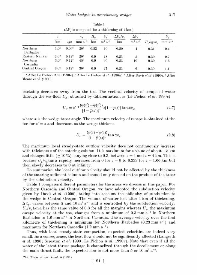
Table 1

(AVw is computed for a thickening of 1 km.)

z vs Hw Vw AVw/v AVVw Uz_ km tgo mm a-l km m2 a-1 km m2 a-1 Uz/tYgvg mm a-1

Northern 1.0a 0.06a 20a 0.53 10 0.20 4 0.31 0.4 Barbados

Eastern Nankai 3.0b 0.12b 20b 0.9 18 0.23 5 0.30 0.7 Northern 3.0" 0.12c 45c 0.9 40 0.23 10 0.30 1.6 Cascadia

Central Oregon 3.0d 0.12d 30c 0.9 27 0.23 6 0.30 1.1

a After Le Pichon et al. (1990c). b After Le Pichon et al. (1990a). " After Davis et al. (1990). d After Moore et al. (1990).

backstop decreases away from the toe. The vertical velocity of escape of water through the sea-floor Uz,, obtained by differentiation, is (Le Pichon et al. 1990c)

=Uz 1 (T(Z') -(z)) z[ 1-Cp(z)] tan avs, (2.7)

where a is the wedge taper angle. The maximum velocity of escape is obtained at the toe for z' = z and decreases as the wedge thickens.

U(z,-5) tan avS. (2.8)

The maximum local steady-state outflow velocity does not continuously increase with thickness z of the entering column. It is maximum for a value of about 1.5 km and changes little (+ 10 %), staying close to 0.3, between z = 1 and z = 4 km. This is because Uz/v tan a rapidly increases from 0 for z = 0 to 0.333 for z = 1.66 km but then slowly decreases to 0 at infinity.

To summarize, the local outflow velocity should not be affected by the thickness of the entering sediment column and should only depend on the product of the taper by the subduction velocity.

Table 1 compares different parameters for the areas we discuss in this paper. For Northern Cascadia and Central Oregon, we have adopted the subduction velocity given by Davis et al. (1990), taking into account the obliquity of subduction to the wedge in Central Oregon. The volume of water lost after 1 km of thickening, AVw, varies between 5 and 10 m2 a-1 and is controlled by the subduction velocity; Uz/vs tan o has the same value of 0.3 for all the margins whereas Uz, the maximum escape velocity at the toe, changes from a minimum of 0.3 mm a-1 in Northern Barbados to 1.6 mm a-1 in Northern Cascadia. The average velocity over the first kilometre of thickening is minimum for Northern Barbados (0.23 mm a-1) and maximum for Northern Cascadia (1.2 mm a-l).

Thus, with local steady-state compaction, expected velocities are indeed very small. As a consequence, the heat flow should not be significantly affected (Langseth et al. 1990; Screaton et al. 1990; Le Pichon et al. 1990c). Note that even if all the water of the latest thrust package is channelized through the decollement or along the main thrust fault, the expected flow is not more than 5 or 10 m2 a-1.

Phil. Trans. R. Soc. Lond. A (1991) [ 91]

317


Are there other possible sources of fluid within the sediment or below the sedimentary column within the oceanic crust ? As discussed by Von Huene & Lee (1983) and more recently by Moore (1989), fluid structurally bound to clay minerals should be released upon burial and heating. Also, the hydrous oceanic crust liberates fluids upon heating (Peacock 1987, this symposium). Below, we briefly show that the order of magnitude expected is less or equal to the values computed above, that is less than a few square metres per year. More important, most of the release of water from smectite occurs at temperatures larger than 60-100 ?C and from the oceanic crust at temperatures larger than 300 ?C and consequently well to the inward side of the accretionary wedge.

Let us first consider the fluid contained within the oceanic crust. Peacock (1987) proposes a conservative volatile content of 2 % in weight for the 8 km thick oceanic crust. Using a density of 3000 kg m-3, this is equivalent to 480Vs m2 a-1 or 10-20 m2 a-l for the wedges considered in table 1. As the estimate of 2 % in weight appears to be conservative these values could possibly be doubled to 20-40 m2 a-. These values are comparable with the total amount of interstitial water released from the wedge in steady state.

Next, we consider the smectite-illite transformation. To get a rough estimate of the amount of water produced by the smectite-illite transformation at temperatures larger than 60 ?C, we assume that three volumes of smectite give two volumes of illite and one of water. According to Tribble (1990), in the Barbados area, the proportion of smectite in the solid phase is 300%. Then, using table 1, we can obtain the additional volume of water produced by transformation of smectite, which would be 1 m2 a-'. Assuming the same proportion of smectite in Oregon, which is certainly an overestimation, we obtain 6 m2 a-l. This value is significant, but is smaller than the original volume of interstitial water. However, at the depth at which this transformation occurs (T > 60 ?C), the low porosity there ensures that the resulting fluid will be much less saline than sea water.

3. Water budget of the Eastern Nankai accretionary wedge The outer Eastern Nankai accretionary wedge has been investigated along a 20 km

section with in situ measurements, observations and samplings coupled with deep tow surveys and surface geophysical observations (Kobayashi et al. 1990; Le Pichon et al. 1990a). Fluid outlets have been identified from the presence of clam colonies, vestimentifera, calcareous concretions, chimneys and white patches. Studies of the chemistry of sea water and interstitial water give qualitative indications on the type of fluid venting whereas instantaneous and long term temperature gradient measurements within the sediments give indirect estimates of the velocity of fluid venting (Foucher et al. 1990a; Henry et al. 1990). An important discovery of this study is that, for a given clam colony type, the range of fluid advection velocities below it is relatively small. Thus an estimation of the surface area occupied by the different types of clams colonies can be converted into a water outflow estimate (Foucher et al. 1990a). Unfortunately, this method could only be used over a zone of fluid venting discovered near the toe of the 4000-3500 m deep outmost thrust unit. Although another important zone of fluid venting was identified at a depth of about 2000 m near the summit of the second 0.6 Ma old thrust unit, the bottom water temperature fluctuations are too large to estimate fluid advection from temperature Phil. Trans. R. Soc. Lond. A (1991)

[ 92 ]

318

Water budgets in accretionary wedges 319

shot points/(50m) -2300 -2220 -2140 -2060 0

i I , i i i i i i i i i I I I O

D -

zone 1 -

- - ^

?

. - -' - 8

D

--8

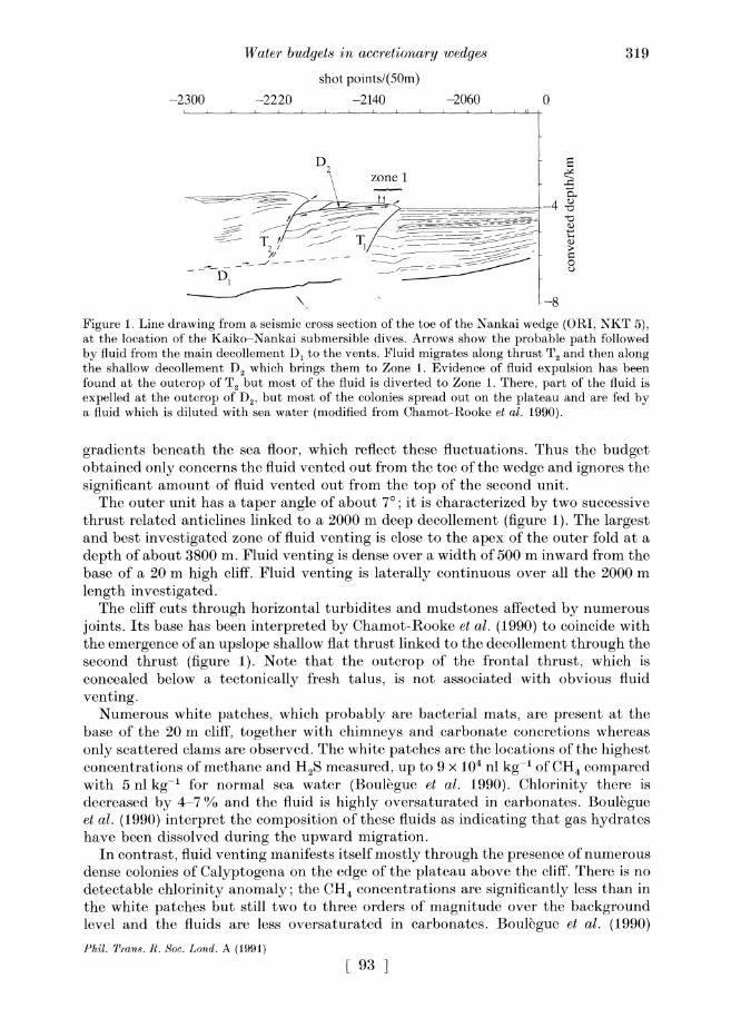
Figure 1. Line drawing from a seismic cross section of the toe of the Nankai wedge (ORI, NKT 5), at the location of the Kaiko-Nankai submersible dives. Arrows show the probable path followed by fluid from the main decollement D, to the vents. Fluid migrates along thrust T2 and then along the shallow decollement D2 which brings them to Zone 1. Evidence of fluid expulsion has been found at the outcrop of T2 but most of the fluid is diverted to Zone 1. There, part of the fluid is expelled at the outcrop of D2, but most of the colonies spread out on the plateau and are fed by a fluid which is diluted with sea water (modified from Chamot-Rooke et al. 1990).

gradients beneath the sea floor, which reflect these fluctuations. Thus the budget obtained only concerns the fluid vented out from the toe of the wedge and ignores the significant amount of fluid vented out from the top of the second unit.

The outer unit has a taper angle of about 7?; it is characterized by two successive thrust related anticlines linked to a 2000 m deep decollement (figure 1). The largest and best investigated zone of fluid venting is close to the apex of the outer fold at a depth of about 3800 m. Fluid venting is dense over a width of 500 m inward from the base of a 20 m high cliff. Fluid venting is laterally continuous over all the 2000 m

length investigated. The cliff cuts through horizontal turbidites and mudstones affected by numerous

joints. Its base has been interpreted by Chamot-Rooke et al. (1990) to coincide with the emergence of an upslope shallow flat thrust linked to the decollement through the second thrust (figure 1). Note that the outcrop of the frontal thrust, which is concealed below a tectonically fresh talus, is not associated with obvious fluid venting.

Numerous white patches, which probably are bacterial mats, are present at the base of the 20 m cliff, together with chimneys and carbonate concretions whereas

only scattered clams are observed. The white patches are the locations of the highest concentrations of methane and H2S measured, up to 9 x 104 nl kg-l of CH4 compared with 5 nl kg-l for normal sea water (Boulegue et al. 1990). Chlorinity there is decreased by 4-7 % and the fluid is highly oversaturated in carbonates. Boulegue et al. (1990) interpret the composition of these fluids as indicating that gas hydrates have been dissolved during the upward migration.

In contrast, fluid venting manifests itself mostly through the presence of numerous dense colonies of Calyptogena on the edge of the plateau above the cliff. There is no detectable chlorinity anomaly; the CH4 concentrations are significantly less than in the white patches but still two to three orders of magnitude over the background level and the fluids are less oversaturated in carbonates. Boulegue et al. (1990) Phil. Trans. R. Soc. Lond. A (1991)

[ 93 ]


AT/mK 0 20 40 60 80 100

location of measurements

20-\ \ ,v? 1,2,3 in the colony \d=l

40-

4 5 112, centre 60 "\,

-

model d=s50 cm d= 00

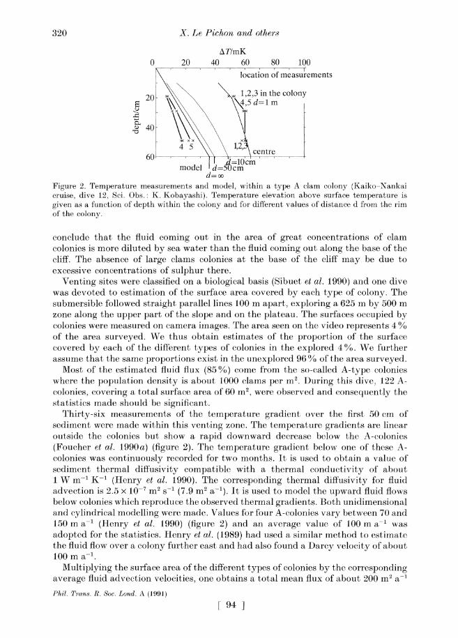
Figure 2. Temperature measurements and model, within a type A clam colony (Kaiko-Nankai cruise, dive 12, Sci. Obs.: K. Kobayashi). Temperature elevation above surface temperature is given as a function of depth within the colony and for different values of distance d from the rim of the colony.

conclude that the fluid coming out in the area of great concentrations of clam colonies is more diluted by sea water than the fluid coming out along the base of the cliff. The absence of large clams colonies at the base of the cliff may be due to excessive concentrations of sulphur there.

Venting sites were classified on a biological basis (Sibuet et al. 1990) and one dive was devoted to estimation of the surface area covered by each type of colony. The submersible followed straight parallel lines 100 m apart, exploring a 625 m by 500 m zone along the upper part of the slope and on the plateau. The surfaces occupied by colonies were measured on camera images. The area seen on the video represents 4 % of the area surveyed. We thus obtain estimates of the proportion of the surface covered by each of the different types of colonies in the explored 4 %. We further assume that the same proportions exist in the unexplored 96 % of the area surveyed.

Most of the estimated fluid flux (85%) come from the so-called A-type colonies where the population density is about 1000 clams per m2. During this dive, 122 A-

colonies, covering a total surface area of 60 m2, were observed and consequently the statistics made should be significant.

Thirty-six measurements of the temperature gradient over the first 50 cm of sediment were made within this venting zone. The temperature gradients are linear outside the colonies but show a rapid downward decrease below the A-colonies (Foucher et al. 1990a) (figure 2). The temperature gradient below one of these A- colonies was continuously recorded for two months. It is used to obtain a value of sediment thermal diffusivity compatible with a thermal conductivity of about 1 Wm-' K- (Henry et al. 1990). The corresponding thermal diffusivity for fluid advection is 2.5 x 10-7 m2 --1 (7.9 m2 a-l). It is used to model the upward fluid flows below colonies which reproduce the observed thermal gradients. Both unidimensional and cylindrical modelling were made. Values for four A-colonies vary between 70 and 150 m a-l (Henry et al. 1990) (figure 2) and an average value of 100 m a-l was adopted for the statistics. Henry et al. (1989) had used a similar method to estimate the fluid flow over a colony further east and had also found a Darcy velocity of about 100 m a-.

Multiplying the surface area of the different types of colonies by the corresponding average fluid advection velocities, one obtains a total mean flux of about 200 m2 a-l


[ 94 ]

320


in the toe area ((100 m a-1 x 60 m2)/(0.04 x 625 m)). This flux ignores the limited amount of venting observed 5 km further inward along the outcrop of the second thrust. It is also limited by the fact that this thermal estimate cannot detect flows of less than 10 m a-1. Finally, as stated above, it ignores the important zone of fluid

venting discovered 10 km further inward near the summit of the second thrust unit.

Consequently, the proposed flux is certainly significantly lower than the actual flux. Yet it is about 40 times larger than the amount obtained assuming local steady-state dewatering.

4. Central Oregon and Northern Cascadia fluid flux estimates

Direct measurements of fluid venting from clam colonies on the toe of the Central

Oregon accretionary wedge are reported by Carson et al. (1990). The fluid appears to come from relatively shallow depth as the methane it contains is biogenic (Kulm & Suess 1990). No decreased salinity has been measured. The obtained Darcy velocities are about 65 m a-l over two vents. Four such vents each having a surface area of about 9 m2 were discovered within an area of the toe that is about 5 by 2 km. The authors have not indicated how much of these 10 km2 were visually explored during their dives but the density of submersible tracks shown suggests that 4% of the 1.5 km wide most densely covered area was explored. If 4 % is a correct proportion, the average flux from this 1.5 km wide portion of the toe is about 40 m2 a-1 whereas the expected local steady-state dewatering would be about 6 m2 a-1 (see table 1). This estimate ignores numerous other less important manifestations of fluid flow such as isolated concentrations of clams, tubeworms and scattered clams (Moore et al. 1990).

Davis et al. (1990) have made 110 closely spaced heat flow measurements over a section of the Northern Cascadia accretionary sedimentary prism off Vancouver Island and compared them with estimates of heat flow based on the depth of a

bottom-simulating reflection (BSR) that is interpreted to mark the thermally controlled base of a methane hydrate layer. They find a systematic discrepancy, the BSR estimated heat flow being about 30 % less than the measured surface heat flow.

They explain the discrepancy through vertical upward fluid advection at an average rate of about 2.5 cm a-1 over a section about 15 km long centred on the toe of the

wedge. The total equivalent flux is about 400 m2 a-1 and should be compared to the

expected local steady-state dewatering which would be about 15 m2 a-1 for a section of 15 km length (see table 1). This last conclusion differs from that of Davis et al.

(1990) who apparently erred in their estimates of flow due to dewatering.

5. Barbados fluid flux estimates

Along the Barbados 15? 30' N section where several holes have been drilled (Moore et al. 1988), heat flow measurements made during drilling reveal high heat flow that

ranges from 96 to 192 mW m-2 in the upper 30-40 m with nonlinear temperature profiles. Below about 100 m, the temperature profiles are linear and the heat flow increases toeward from 40 to 90 mW m-2 (Fisher & Hounslow 1990). The upper high temperature gradient anomalies have been interpreted by Fisher & Hounslow (1990) as due to rapid transient fluid flow of water along faults. Sea-floor venting in faulted areas is confirmed by local surface heat flow anomalies at a scale of a few hundreds of metres which requires flows of a few tens of square metres per year (Foucher et al.


[ 95]

321

1990b; Lallemant et al. 1990). The deeper linear gradients were interpreted as due to flow along the decollement at velocities of about 10 m a-1 (Fisher & Hounslow 1990; Foucher et al. 1990 b). The resulting seaward fluid flow along the decollement would be about 400 m2 a-l (Foucher et al. 1990b). Fluid, sampled both in the decollement and near active faults, has a salinity reduced by 10-30 % with respect to normal sea water (Gieskes et al. 1990). Near 12? 20' N, small-scale high heat flow anomalies also coincide with sea-floor faulted areas and can be explained by surface venting of a few tens of square metres per year (Foucher et al. 1990). Two heat flow transects near 14? 20' N and 14? 35' N did not reveal any broadscale anomalies of high heat flow, but again showed some locally high values possibly associated with faults (Langseth et al. 1990).

Additional remarkable evidence for large-scale fluid venting was reported by Le Pichon et al. (1990b). They describe a 0.55 km2 oval shaped mud volcano near 13? 50' N, 12 km seaward of the Barbados accretionary complex deformation front, through which about 106 m3 of fluid are advected upward every year, with a maximum upward Darcy velocity at the axis of 17 m a-1. This estimate is based both on thermal and chemical considerations. The interstitial water sampled in the mud- volcano is half as saline as normal sea water. The edge of the mud volcano is more than 30000 and less than 100000 years old. The mud volcano is part of a large field of mud volcanoes there and implies a very large amount of lateral drainage at depth as, in steady state, the water, if it were produced by compaction, would correspond to the production of a 100 km length along strike of wedge.

The Barbados evidence thus indicates both the existence of large-scale seaward flow at depth along the decollement of deep originated less saline water, up to two orders of magnitude above local steady-state compaction estimates, and more local, possibly transient, surface anomalies implying advection of a few tens of square metres per year.

6. Discussion

We have shown that submersible investigations indicate the existence of fluid seeps on a scale of a few square metres. Indirect measurements based on subsurface temperature gradients (Foucher et al. 1990a; Henry et al. 1990) as well as direct measurements (Carson et al. 1990), indicate fluid flow velocities of the order of 100 m a-1. However, thermal measurements in the first 50 cm of sediment cannot be used to estimate upward fluid velocities of less than 10 m a-1. On the other hand, investigations made from the surface ships with heat flow probes indicate wider (100 m to a few kilometres) but much smaller heat flow anomalies with an increase over the background heat-flow of 30-100 %, corresponding to surface flow velocities of a few centimetres per year to 10 m a-1 at most. However, pogo-stick-type thermal measurements can only be used to measure distributed and slow intergranular flow, not only because the probability to hit a vent is quite low (about 1 % in a known active zone) but also because thermistors are usually too deep to detect the shallow curvature of the temperature profiles measured within vents.

One could argue that localized venting of large amounts of fluids should increase significantly the conductive heat flow outside the vents, which can be measured both from sea surface as well as during submersible investigations. However, in the deepest zone explored during the Kaiko-Nankai cruise (referred to as Zone 1), no significant increase of the background heat flow has been observed in the area of active venting. We show below that this result implies that deep originated fluids


[ 96 1

322 X. Le Pichon and others


flow laterally into the venting area and are then diluted with sea water before they reach the clam colonies.

(a) Necessity of lateral fluid input The total heat flux Fs though the surface of the active area on the plateau in Zone

1 can be expressed as the sum of two terms, one corresponding to the gradient outside the colonies, the other to the heat flux through clam colonies

Fs = ASfo + (pc)f OQ, (6.1)

where A is the thermal conductivity (about 1 W m-l K-1), S is the surface area of the active area on the plateau (300 m2 per m of subduction zone), f0 is the thermal gradient outside colonies (60 mK m-l), (pc)f is fluid volumetric heat capacity (4 x 106 J m-3), Qc is the fluid flux through clam colonies (about 200 m2 a-l) and 0 is the characteristic temperature elevation inside clam colonies. 0 is of the order of 0.1 ?C at most. In the following discussion, we also use thermal diffusivity D =

A/(pc)f (7.9 m2 a-). Note that with these parameters, heat expelled by fluid advection in clam colonies is seven times smaller than conductive heat flux outside clam colonies integrated over the active area.

If all the fluid flowing through clam colonies is seeping vertically from deep below the colonies, a model with uniform fluid advection at Darcian velocity Qc/S in a uniform half-space can be used. Then, temperature at any depth z is:

T(z) = T (1 -exp (-z/h)), (6.2)

where h = SD/QC = 12 m (6.3) and as Fs = (pc)f T Q, T,, = 0+hfo = 0.81 ?C. (6.4)

Surface temperature is here taken as zero. The temperature of the fluid source compatible with this model is To. This corresponds to a very shallow depth (13.5 m), which implies that deep fluids are cooled, either by conduction or dilution. As a first step, we will determine the amount of cooling that can be expected from conduction to the sediment surface outside the area of venting if fluids come laterally.

(b) Fluid cooling along a sloping aquifer of low dip angle A shallow decollement (or low-angle thrust) outcrops near the top of the slope,

20 m below the top of the frontal thrust anticline (Chamot-Rooke et al. 1990). This decollement connects with the second major thrust (see figure 1). Its dip angle can be constrained from seismic reflection data and is about 4?. The taper angle a of the

overlying wedge is fairly constant at about 7?. Assuming steady state and neglecting horizontal heat transfer, temperature along the fluid path from the deep decollement to the feeding thrust fault and then to the shallow decollement which feeds Zone 1 vents (see figure 1) can be calculated. We assume for the shallow decollement below the main cluster of clam colonies a depth of 30 m. The temperature of the incoming fluids Tf is then computed (see Appendix A).

For a fluid flux Qr along the shallow decollement smaller than 40 m2 a-l, the

gradient increase due to fluid flow along this decollement is moderate and, below the surface zone of outflow, does not depend on the temperature of the fluid source. If fluids flowing out of clam colonies were undiluted (Qr = Qc = 200 m2 a-l), the

approximation used no longer applies and very high heat flows of more than 300 mW m-2 are predicted by the exact solution (see Appendix A). It follows that the


[ 97 ]

323

14 Vol. 335. A


fluid flux Qr along the shallow decollement cannot be of the same order of magnitude than the fluid flux observed in clam colonies. This implies that fluids from the deep source are diluted with sea water before they reach the colonies.

(c) Dilution models

For a given fluid dilution factor d = Qc/Qr, both the sloping aquifer model and the unidimensional advection model give ranges of values for the temperature at the depth of the shallow decollement. It is thus possible to determine the probable amount of dilution by looking for the compatibility domain of these two models.

Mixing with sea water occurs within the shallow decollement at depth H. Thus, upward flow from decollement to the surface is equal to Qc/S and temperature at

depth 0 to H is given by equation (6.2). As explained in Appendix B a relationship between temperature in the decollement below the colonies and the temperature of

incoming fluids can be obtained from the heat balance equation at the shallow decollement level.

But the structure of the temperature field in and around clam colonies has been interpreted as an indication that recharge with sea water occurs at a shallow depth (1 or 2 m), implying local convection around the colonies (Henry et al. 1990). We consequently consider another case when dilution occurs by convection near the surface. We assume that a uniform advection model applies in the domain between the shallow decollement and the base of the convection cells (see Appendix B). Then, the temperature predicted in the shallow decollement by this model must be equal to the temperature T of incoming fluids.

Comparing these two models, convection near the surface requires higher dilution than mixing in the decollement, the actual dilution factor being most probably between 6 and 15. Temperature in the decollement should be very low if sea water is flowing into it, but should not be anomalous if dilution occurs near the surface. On the other hand conductive heat flow is expected to be significantly higher than normal north of the active zone if mixing occurs in the decollement as the predicted temperature for incoming fluid is higher.

(d) Numerical estimates of dilution

When applying either model, the major source of uncertainty is the value of f, the thermal gradient below the shallow decollement, which is supposedly equal to the 'regional' gradient.

There are few measurements which can be used as references for heat flow. One measurement made in the trench between Tenryu Canyon and Zenisu ridge gives 67 mW m-2 (Nahihara et al. 1989). As conductivity is in the range 0.7-1.3 W m-1 K-1 but more probably around 1 W m-l K1, this value is quite compatible with the measured gradient of 60 mK m-1 in the toe area. Measurements were recently made closer to the Kaiko-Nankai area (Kinoshita & Kazumi 1990) on the lower tectonic unit to the northeast. At the northeastern extremity, the thermal gradient is 60 mK m-1, while closer to the explored area but near the base of the upper tectonic unit, the thermal gradient is low, around 40 mK m-l. In the absence of fluid advection, heat flow tends to decrease landward because of tectonic thickening of sediments in the wedge, and because of the slab burial effect (Toksoz et al. 1975; Le Pichon et al. 1990c; Molnar & England 1990). As Zone I is much closer to the deformation front, a surface gradient value of 40 mK m-l probably determines an absolute minimum for heat flow coming from below the shallow decollement.


[ 98

324


For a value of the background gradient of 40 mK m-l, dilution should be between 6.5 and 9; for 50 mK m-l, between 10 and 15; for 60 mK m-1, between 20 and more than 30, but this last determination is also very dependent on other parameters such as thermal conductivity, aquifer slope and aquifer depth below the active zone.

Salinity contrast, rather than temperature gradient, is probably driving convection (Henry et al. 1990). As noted earlier, fluids originated from deep within an accretionary complex tend to have a low salinity, but the actual salinity of

incoming fluids is not known in the Kaiko-Nankai area. A salinity difference of a few

per mil between sea water and source is enough to start convection if conduit

permeability is high, but the major constraint is that flow in the conduit, at a

velocity of 100 m a--1, has then to be driven by buoyancy of the diluted fluids.

Assuming that fluids have, after dilution, a density a few grams per litre less than sea water, conduit permeabilities of the order of 10-10 m2 are required (Henry et al. 1990). Dilution factors of more than 10 are thus unlikely.

(e) Applicability to other wedges The model proposed for Kaiko-Nankai area might be applied to the 12? N section

of the Barbados accretionary wedge, as the context is somewhat similar. There, fluids

presumably flow along a major thrust into a shallow decollement, and are expelled through faults in the overlying thrust outcrop wedge of deformed sediment (Foucher et al. 1990b). The corresponding heat flow increase is moderate (40 %), indicative of a deep fluid flux of the order of 20 m2 a-1. However, we do not know if vents are

present on these thrust outcrop wedges and consequently whether there is some convection.

In the Oregon diving sites, the venting fluids are probably diluted, as their salinity is normal and as the large amount of fluid flux is not compatible with local shallow sources. Then convection would occur between the surface and permeable sand strata

acting as conduits for lateral migration. As in the Kaiko-Nankai area, major vents with associated clam colonies were found at the top of the anticline, but other types of vents were also found in association with permeable sand strata on the eroded

slope just below the active zone. However, the very high heat flow at depth in the toe area of the Barbados Ocean

Drilling Project (ODP) profile indicates that a large amount (a few 100 m2 a-l) of deep originated low salinity fluid flows there along the decollement (Foucher et al. 1990b; Langseth et al. 1990). Recent transient fluid flow has been proposed to explain high surface heat flows (Fisher & Hounslow 1990) but this does not account for the overall increase of the gradient at depth. Furthermore, the huge amount of fluid expelled through the mud volcano area at 130 50' N requires lateral flow at a 100 km scale. This leaves us with the problem of explaining the origin of tens of square metres per year of low salinity water at depth and their subsequent large-scale transient transport.

The widespread fluid flow (of the order of 400 m2 a-l) out of the Northern Cascadia

wedge (Davis et al. 1990) cannot be explained either way, but one may ask what confidence can be given to the temperature estimated at the base of the hydrate layer as the exact composition of the hydrates is not known.


325

[ 99 ] 14-2


7. Conclusion

We have shown that on the Eastern Nankai area very large fluid outflows measured on the toe of the accretionary wedge include a large component of locally derived sea water, probably resulting from haline convection. However, the amount of low salinity water necessary to drive this convection is still of the same order of magnitude as the water produced by compaction of the whole sedimentary column. In the Barbados area previous work has given further evidence for large-scale flow of low salinity water along the decollement, this flow being an order of magnitude larger than possible flow from compaction of the whole sedimentary column.

Where does the large amount of low salinity water come from ? The smectite-illite transformation and the hydrate layer are obvious sources but cannot provide amounts larger than a few square metres per year to at most 10 m2 a-. Another possible source is the oceanic crust if it includes a sizeable thickness of serpentinized peridotite. For example 2 km of 50 % serpentinized peridotite would contain more water than the sedimentary column. This source would not be sufficient if the amount of low salinity water required is indeed larger than a few tens of square metres per year in steady state. Then, one would have to invoke long distance transport of fresh water from the adjacent subaerially exposed basins and (or) exotic recharge mechanisms such as the seismic pumping mechanism (Sibson et al. 1975).

Appendix A. Model of fluid flow along an aquifer

Steady state is assumed and diffusion along the horizontal (x) axis is neglected. The geometry is as shown on figure 3. The aquifer is thin, so that the fluid

temperature T(x) is uniform across it. The depth of the aquifer below the surface is H(x). The fluid flux in the aquifer is Q. In steady state, heat flow below the aquifer is unaffected by the fluid flow because all the additional heat must be conducted

upward to the surface. Thus we assume that the heat flow below the aquifer is uniform and constant, equal to the heat flow at the surface in the absence of fluid flow. As we also assume a uniform thermal conductivity (A), the temperature gradient below the aquifer (f) is a constant. Because horizontal heat diffusion is

neglected, the temperature profile between the aquifer and the surface is linear and the gradient above the aquifer is Tf/H. The heat lost by water flowing along the

aquifer is then related to the discontinuity of gradient across the aquifer by the

following equation (pc)W Q dT/dx = A[Tf/H(x)-f . (A 1)

Solutions of this equation can be determined easily if the dip (a) of the aquifer is constant. With H(x) = tan ax, (A 1) becomes

Tf-vT/x =- vtan f, (A 2)

where v = A/(pc)w Q tan a. (A 3)

For v # 1, its solutions are

T(z) = Cz"+ (v/(v-l))fz, (A 4)

where C is a function of v and of the temperature at the deep end of the aquifer.


[ 100 ]

326


z I z

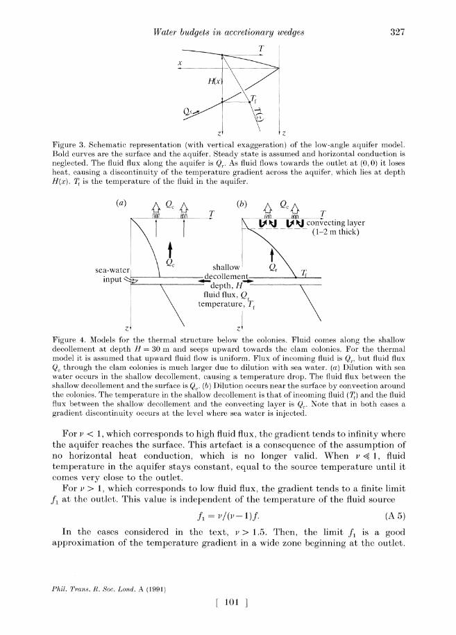
Figure 3. Schematic representation (with vertical exaggeration) of the low-angle aquifer model. Bold curves are the surface and the aquifer. Steady state is assumed and horizontal conduction is neglected. The fluid flux along the aquifer is Qr. As fluid flows towards the outlet at (0, 0) it loses heat, causing a discontinuity of the temperature gradient across the aquifer, which lies at depth H(x). T, is the temperature of the fluid in the aquifer.

(a) Q)M c b T Q ! ^

\\ \ 1V kJ 1 VJ convecting layer r\ IX I

-\ - --_- _(1-2 m thick)

t \ sea-water shallow Q input - decollement i -n \ depth, H

fluid flux, Qr temperature, Tf

z' z

Figure 4. Models for the thermal structure below the colonies. Fluid comes along the shallow decollement at depth H = 30 m and seeps upward towards the clam colonies. For the thermal model it is assumed that upward fluid flow is uniform. Flux of incoming fluid is Qr, but fluid flux Qo through the clam colonies is much larger due to dilution with sea water. (a) Dilution with sea water occurs in the shallow decollement, causing a temperature drop. The fluid flux between the shallow decollement and the surface is Qc. (b) Dilution occurs near the surface by convection around the colonies. The temperature in the shallow decollement is that of incoming fluid (T,) and the fluid flux between the shallow decollement and the convecting layer is Qr. Note that in both cases a gradient discontinuity occurs at the level where sea water is injected.

For v < 1, which corresponds to high fluid flux, the gradient tends to infinity where the aquifer reaches the surface. This artefact is a consequence of the assumption of no horizontal heat conduction, which is no longer valid. When v < 1, fluid temperature in the aquifer stays constant, equal to the source temperature until it comes very close to the outlet.

For v > 1, which corresponds to low fluid flux, the gradient tends to a finite limit fi at the outlet. This value is independent of the temperature of the fluid source

fi = /(vp-1)f. (A 5)

In the cases considered in the text, v > 1.5. Then, the limit f, is a good approximation of the temperature gradient in a wide zone beginning at the outlet.


[ 101 ]

327


Appendix B. Dilution models

These models are based on the two following assumptions. Fluids come into the area of active venting laterally, along a shallow slightly dipping aquifer. A unidimensional advection model can be used to describe the temperature profile between this aquifer and the surface in the area of venting (See figure 4).

The temperature of fluids coming along the aquifer is known from the model explained in Appendix A. It can be computed from equation (A 5),

Tf- v/(v-1)Hf, (B 1)

where H (30 m) is the depth of the shallow decollement below the zone of active

venting. Very generally, the temperature profile resulting from uniform upward advection

of fluid at velocity U in a half-space of thermal uniform thermal diffusivity D (D =

A/(pc)w) is T(z) = Tsurface + TO [1 -exp (-Uz/D)] (B 2)

For simplicity, we take Tsurace = 0. The total heat flow, including advection and conduction is uniform in the half-

space, and equals (pc)f UTimit. In particular, it must be equal to the heat flow measured at the surface. Let us define Ta = Fs/(pc)f Qc where Fs is the total heat flux

through the surface in Zone 1, as defined in (6.1). We have

(pc)f Qc Ta = FS = (pc) SUT. (B 3)

Then two end-member cases are considered, in one case dilution occurs near the surface, thus SU = Qr and, from (B 3), To = T Qc/Qr. In the other case dilution occurs in the shallow decollement, thus SU = Qc and, from (A 3), T, = Ta. As in (6.3), let us define h = DS/Qc and d = Qc/Qr. The temperature as a function of depth is, for the model with shallow convection,

T(z) = dl/[1 - exp (- z/dh)] (B 4)

and for the model with mixing in the shallow decollement,

T(z) = 7[1- exp (-z/h)]. (B 5)

The next step is to relate the temperature T(H) in the shallow decollement

predicted by the uniform advection model with the temperature Tf of incoming fluids. If mixing with sea water occurs near the surface, one obviously has

T(H) = Tf. (B 6)

If mixing occurs in the shallow decollement, the heat balance across the decollement must be considered. The conductive flux from below is AfS, the heat input due to fluid flow along the shallow decollement into the zone of venting is (pc)w Qr Tf and the heat flux above this aquifer is equal to the flux through the surface Fs. Thus

T, = Tf/d+DSf/QC. (B 7)

We finally obtain for each case a set of equations which determines the dilution factor d from known parameters.

Note that, rigorously, the heat balance at the decollement should also be applied to the model with dilution near the surface. In this case, it implies continuity of the


[ 102 ]

328


temperature gradient across the aquifer. This additional condition theoretically determines the value of F. However, this condition is not satisfied exactly, as the actual fluid flow pattern is not strictly one dimensional. In particular, part of the fluids continue to flow along the aquifer and release some heat. Thus we tolerate

gradient discontinuities of the order of 10 mK m-1.

References

Boulegue, J., Aquilina, L., Mariotti, A., Gamo, T. & Sakai, H. 1990 Chemistry of fluids in the Kaiko-Nankai area (Nankai accretionary prism). Int. Conf. Fluids in Subduction Zones (Abst.), Paris, 5-6 November 1990.

Bray, C. J. & Karig, D. E. 1985 Porosity of sediments in accretionary prisms and some implications for dewatering processes. J. geophys. Res. 90, 768-778.

Carson, B., Suess, E. & Strasser, J. C. 1990 Fluid flow and mass flux determinations at vent sites on the Cascadia margin accretionary prism. J. geophys. Res. 95, 8891-8897.

Chamot-Rooke, N., Lallemant, S., Henry, P., Le Pichon, X., Cadet, J. P. & Lallemand, S. 1990 Tectonic context of fluid venting at the toe of the Nankai Accretionary Prism (Kaiko-Nankai diving cruise). Int. Conf. Fluids in Subduction Zones (Abstr.), Paris, 5-6 November 1990.

Davis, E. E., Hyndmann, R. D. & Willinger, H. 1990 Rates of fluid expulsion across the Northern Caseadia Accretionary Prism: constraints from new heat flow and multichannel seismic reflection data. J. geophys. Res. 95, 8869-8889.

Fisher, A. T. & Hounslow, M. W. 1990 Transient fluid flow through the toe of the Barbados accretionary complex: constraints from ocean drilling program Leg 110 heat flow studies and simple models. J. geophys. Res. 95, 8845-8859.

Foucher, J. P., Henry, P., Sibuet, M., Kobayashi, K. & Le Pichon, X. 1990a Heat flow and fluid budget at the toe of the Nankai accretionary prism near 138? E. Int. Conf. Fluids in Subduction Zones (Abstr.), Paris, 5-6 November 1990.

Foucher, J. P., Le Pichon, X., Lallemant, S., Hobart, M. A., Henry, P., Benedetti, M., Westbrook, G. K. & Langseth, M. G. 1990b Heat flow, tectonics and fluid circulation at the toe of the Barbados Ridge accretionary prism. J. geophys. Res. 95, 8859-8868.

Gieskes, J. M., Vrolijk, P. & Blanc, G. 1990 Hydrogeochemistry of the Barbados accretionary wedge transect: Ocean Drilling Project Leg 110. J. geophys. Res. 95, 8809-8818.

Henry, P., Lallemant, S., Le Pichon, X. & Lallemand, S. 1989 Fluid venting along Japanese trenches: tectonic context and thermal modeling. Tectonophys. 160, 277-291.

Henry, P., Foucher, J. P., Le Pichon, X., Lallemant, S. & Chamot-Rooke, N. 1990 Thermal modelling of clam colonies: fluid flow velocity estimates from Kaiko-Nankai thermal data. Intn. Conf. on Fluids in Subduction Zones, Paris, 5-6 November 1990, Abstract.

Kinoshita, M. & Kazumi, Y. 1988 Heat flow - basic data. In Preliminary report of the Hakuho-Maru cruise KH 86-5 (ODP site survey) (ed. A. Taira), pp. 51-76. Tokyo: ORI.

Kobayashi, K. et al. 1990 General description of the Kaiko-Nankai Project. Intn. Conf. on Fluids in Subduction Zones, Paris, 5-6 November 1990, Abstract.

Kulm, L. D. & Suess, E. 1990 Relationship between carbonates deposits and fluid venting: Oregon accretionary prism. J. geophys. Res. 95, 8899-8916.

Lallemant, S., Henry, P., Le Pichon, X. & Foucher, J. P. 1990 Detailed structure and possible fluid paths at the toe of the Barbados accretionary wedge (ODP Leg 110 area). Geology 18, 854-857.

Langseth, M. G., Westbrook, G. K. & Hobart, M. 1990 Contrasting geothermal regimes of the Barbados Ridge accretionary complex. J. geophys. Res. 95, 8829-8844.

Le Pichon, X. et al. 1990a Fluid venting in easternmost Nankai accretionary prism based on Kaiko-Nankai cruise results. Intn. Conf. on Fluids in Subduction Zones, Paris, 5-6 November 1990, Abstract.

Le Pichon, X., Foucher, J. P., Boulegue, J., Henry, P., Lallemant, S., Benedetti, F., Avedik, F. & Mariotti, A. 1990 b Mud volcano field seaward of the Barbados accretionary complex: a submersible survey. J. geophys. Res. 95, 8931-8945.


[ 103 1

329


Le Pichon, X., Henry, P. & Lallemant, S. 1990c Water flow in the Barbados accretionary complex. J. geophys. Res. 95, 8945-9868.

Molnar, P. & England, P. 1990 Temperatures, heat flux, and frictional stress near major thrust faults. J. geophys. Res. 95, 4833-4856.

Moore, J. C. et al. 1988 Tectonics and hydrogeology of the northern Barbados Ridge, results from the Ocean Drilling Program Leg 110. Geol. Soc. Am. Bull. 100, 1578-1593.

Moore, J. C. 1989 Tectonics and hydrogeology of accretionary prisms: role of the decollement zone. J. struct. Geol. 11, 95-106.

Moore, J. C., Orange, D. & Kulm, L. D. 1990 Interrelationship of fluid venting and structural evolution: Alvin observations from the frontal accretionary prism: Oregon. J. geophys. Res. 95, 8795-8808.

Nagihara, S., Kinoshita, H. & Yamano, M. 1989 On the high heat flow in the Nankai Trough area - A simulation study on a heat rebound process. Tectonophys. 161, 33-41.

Peacock, S. M. 1987 Thermal effects of metamorphic fluids in subduction zones. Geology 15, 1057-1060.

Screaton, E. J., Wuthrich, D. R. & Dreiss, S. J. 1990 Permeabilities, fluid pressures and flow rates in the Barbados ridge complex. J. geophys. Res. 95, 8997-9007.

Sibson, R. H., Moore, J. McM. & Rankin, A. H. 1975 Seismic pumping - a hydrothermal fluid transport mechanism. J. geol. Soc. Lond. 131, 653-659.

Sibuet, M., Fiala, A., Foucher, J. P. & Ohta, S. 1990 Spatial distribution of clams colonies at the toe of the Nankai accretionary prism near 138? E. Int. Conf. on Fluids in Subduction Zones, Paris, 5-6 November 1990, Abstract.

Toksoz, M. N., Minear, J. W. & Julian, B. R. 1971 Temperature fields and geophysical effects of a downgoing slab. J. geophys. Res. 76, 1113-1138.

Tribble, J. S. 1990 Clay diagenesis in the Barbados accretionary complex: potential impact on hydrology and subduction mechanics. In Proc. ODP, Sci. Results (ed. J. C. Moore et al.) 110, 97-110. College station, Texas: Ocean Drilling Program.

Von Huene, R. & Lee, H. 1983 The possible significance of pore fluid pressure in subductions zones. In Studies of continental margin geology. Mem. Am. Ass. Petrol. geol. 34, 781-791.

Phil. Trans. R. Soc. Lond. A (1991) [ 104 ]

330

water budgets in accretionary wedges: a comparison

Documents