Water-Quality Indices

for Specific Water Uses

GEOLOGICAL SURVEY

CIRCULAR 770

Water-Quality Indices for Specific Water Uses

By J. D. Stoner

GEOLOGICAL SURVEY CIRCULAR 770

1978

United States Department of the InteriorCECIL D. ANDRUS, Secretary

Geological SurveyH. William Menard, Director

Free on application to Branch of Distribution, U.S. Geological Survey, 1200 South Eads Street, Arlington, VA 22202

CONTENTS

PageAbstract_____________________________ 1Introduction _ ___ _ __ _ _ ______ _ ___ ___ _ 1Earlier indices _________________________ 1Development of the index_________ _________ 2

Criteria ____________________________ 2Boundary conditions __________________ 2Mathematical functions ______ _ __ _____ _ _ 2Types of properties ___-______________ 3

Type-I properties__________________ 3Type-II properties ________________ 4

Index __________________ ____ 4

Page

Examples of specific indices __ _, _______ _____ 5 Public water supply index _ _ _ _ ___ _ _ _ _ 5

Type-I properties_________________ 5Type-II properties __________________ 5Application of index _______________ 8

Irrigation index ____________________________ 8Type-I properties_____________ ___ 10Type-II properties ___________________ 10Application of index _____________________ 10

Conclusions ________________________________ 10References___________________________ 12

ILLUSTRATION

FIGURE 1. Plot of the function QF=a+bX2 for constituent A.____________________________________________ 3

TABLES

TABLE 1. Type-I properties selected for public water supply index____-___--____-_____-__________________ 52. Type-II properties selected for public water supply index ______________________________________ 53. Recommended maximum fluoride concentrations _____ ________________________________________________ 74. Type-II property effects for the public water supply index ___________________________________ 85. Public water supply indices and individual property effects for selected waters _________________________ 96. Type-I properties for the irrigation index _________^.-____-___-______-_____________________ 107. Type-II properties for the irrigation index ___________________________________________________________ 118. Irrigation indices and individual property effects for selected waters ___________________________________ 11

Hi

Water-Quality Indices for Specific Water Uses

By JERRY D. STONER

ABSTRACT

Water-quality indices were developed to assess waters for two specific uses public water supply and irrigation.The as­ sessment for a specific water use is based on the availability of (Da set of limits for each water quality property selected, (2) a rationale for selection, and (3) information that permits one to appraise the relationship of the concentration of the selected property to the suitability of the specific water use. The selected properties are divided into two classes: Type-I prop­ erties, those normally considered toxic at low concentrations, and type-II properties, those which affect aesthetic conditions or which at high concentrations can be considered toxic or would otherwise render the water unfit for its intended use.

In the method used, type-I properties affect the index only when their recommended limits are exceeded. The type-II properties affect the value of the index over the complete range, from optimum or ideal concentrations to concentrations exceeding their respective recommended limits. The index value is the summation of the type-I and type-II effects. The range of the index is such that the value 100 represents a perfect water, zero a water that has the aggregate effect of the properties at their recommended limits, and a negative value a water unfit for the use intended without further treatment.

The index is designed to (1) provide numbers so that various waters can be compared directly with one another, (2) allow for comparison of water-quality changes with time, (3) indi­ cate waters of both "good" and "bad" quality, and (41 provide values which managers and other nontechnical personnel can use more easily to characterize water quality. The method developed can be applied to water-quality indices for specific uses that are very broad or very narrow in scope.

INTRODUCTION

At the present time an increased emphasis has been placed upon the development of water- quality indices. Much of the effort in developing quality indices is directed toward quantifying such terms as "good" and "bad," and the values between these extremes. In this context, a water-quality index is a grading system for com­ parison of various waters.

A water-quality index is also the summation of the individual effects of the several properties

used to develop the index. This attribute of an index allows direct comparison of the overall quality of different waters even though the con­ centration ranges of the individual constituents may be very different. These two attributes, the quantification of "good" and "bad" and the sum­ mation of individual effects, allow the user to ex­ amine waters and view them in terms of ranked order for example; bad, poor, good, better, best. The water-quality index is also a method of pro­ viding water-quality information that can be more readily used by planners, managers, and other nontechnical people. In general, managers and planners will have technical staffs to analyze the raw data. However, the technical analyses must still be presented to the managers and plan­ ners in a form they can understand and use. The water-quality index is a useful tool in bridging this information gap.

The water-quality index can be a good tool for presenting water-quality data. It can be used in trend analyses, graphical displays, and in tabular presentations. It is an excellent format for sum­ marizing overall water-quality conditions over space and time.

This report presents a new concept in the devel­ opment of water-quality indices. Application of the method to a wide range of use categories and waters should show its utility and test the va­ lidity of the concept. The method should not be construed to be an official U.S. Geological Survey technique.

EARLIER INDICES

A general water-quality index not directed to­ ward any specific water use was developed and reported by Brown, McClleland, Deininges, and Tozer (1970). They concluded that a single numer-

ical expression reflecting the composite influence of significant properties of water quality is feasi­ ble.Various investigators have developed water- quality indices for specific uses. Amongst the oldest is the classification scheme for irrigation waters by Wilcox (1955). More recently, Harkins (1974) developed an index specifically for use in trend analysis, and Walski and Parker (1974) de­ veloped an index to be applied to recreational use.

DEVELOPMENT OF THE INDEX

Classification of waters according to specific uses has become increasingly important. Apply­ ing a general water-quality index to specific-use waters may lead to conclusions that are not en­ tirely valid, primarily because the importance and influence of water-quality properties vary for different uses. As an example, water temperature is relatively unimportant in water used for irriga­ tion but is of vital importance in waters used for the maintenance of aquatic life. With the method to be described, a water-quality index for any water use, broad or narrow in scope, can be devel­ oped if certain information can be provided. The minimum information needs are (1) a set of limits for each water-quality property to be considered,(2) a rationale for establishment of the limits, and(3) some information on, or appraisal of, the rela­ tion of various concentrations of each property to the specific water use for which the index is being developed.

Two broad water-use categories, public water supply and irrigation, were analyzed to develop the method. The National Academy of Sciences and National Academy of Engineering report, "Water Quality Criteria 1972" (1972), provided the necessary information for the development of the water-use indices.

The water-quality properties, rank order, weighting factors, and mathematical expressions used in this report are the author's subjective choices based upon his experience and the Na­ tional Academy of Sciences report, and as such, they will probably not be accepted by all readers. All developers of indices face the problem of sub- jectiveness. The DELPHI method, as used by Brown, McClleland, Deininges, and Tozer (1970) could be applied to the procedure developed in this report to reduce subjectiveness.

CRITERIA

Two criteria were adopted to develop a base from which a specific-use index could be gen­ erated. The first criterion was that the number generated as the index value from one water must be directly comparable to the index number gen­ erated from a different water. The second criter­ ion was that the number generated should repre­ sent the "fitness" of the water for the specific-use category under consideration. These criteria dif­ fer from the criteria of other indices in that most indices developed to date have been concerned with judging waters in terms of general overall quality that is, how "good" the waters are irrespective of their intended use.

BOUNDARY CONDITIONS

In order to meet the established criteria, the QF's (quality function), which are the mathemat­ ical functions representing individual water- quality properties making up the WQI (water- quality index), and the WQI itself assign to an "ideal" water the arbitrary value of 100. Because of the method of computation, the boundary con­ ditions for the individual properties were applied to the respective QF's. The QF's and WQI for a water at the recommended concentration limits were arbitrarily set at zero. In this way, when the QF's or WQI (which is the sum of the individual effects), are somewhere in the range of 0 to 100, the "goodness" of the water for a specific use can be judged. The QF of an individual property whose value has exceeded the limit becomes negative. The more the limit is exceeded, the larger the negative number becomes. No limit is placed upon the value that a negative number can become. If the sum of the individual effects is negative, then the WQI becomes negative. Thus, if the value of a property normally not considered toxic at commonly found concentrations reaches a toxic concentration, or if a concentration renders the water unfit for use, the value will make the WQI negative.

MATHEMATICAL FUNCTIONS

Mathematical functions instead of graphical descriptions were chosen to describe the effect of the water-quality properties upon the index.

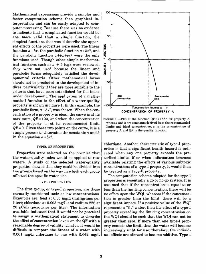
Mathematical expressions provide a simpler and faster computation scheme than graphical in­ terpretation and can be easily adapted to com­ puter processing. Because there was no evidence to indicate that a complicated function would be any more valid than a simple function, the simplest functions that would describe the appar­ ent effects of the properties were used. The linear function a +bx, the parabolic function a+bx2 , and the parabolic function a+bx+cx2 were the only functions used. Though other simple mathemat­ ical functions such as a + b logx were reviewed, they were not used because the linear and parabolic forms adequately satisfied the devel­ opmental criteria. Other mathematical forms should not be precluded in the development of in­ dices, particularly if they are more suitable to the criteria that have been established for the index under development. The application of a mathe­ matical function to the effect of a water-quality property is shown in figure 1. In this example, the parabolic form, a+bx2 , was chosen. When the con­ centration of a property is ideal, the curve is at its maximum, QF=100, and when the concentration of the property is at its recommended limit, QF=0. Given these two points on the curve, it is a simple process to determine the constants a and 6 in the equation a+bx2 .

TYPES OF PROPERTIES

Properties were selected on the premise that the water-quality index would be applied to raw waters. A study of the selected water-quality properties showed that they could be divided into two groups based on the way in which each group affected the specific water use.

TYPE-I PROPERTIES

The first group, or type-I properties, are those normally considered toxic at low concentrations. Examples are: lead at 0.05 mg/L (milligrams per liter); chlordane at 0.003 mg/L and radium 226 at 20 pCi/L (picocuries per liter). The information available indicated that it would iwt be practical te assign a mathematical statement to describe the effect of concentration levels on the QF with a reasonable degree of validity.-That is, it would be difficult to compare the fitness of a water with 0.001 mg/L chlordane to one with 0.092 mg/L

-100Concentration Increases >

CONCENTRATION OF PROPERTY A

FIGURE 1. Plot of the function QF=a+bX2 for property A, where a and 6 are constants derived from the recommended limits and ideal concentration, x is the concentration of property A and QF is the quality function.

chlordane. Another characteristic of type-I prop­ erties is that a significant health hazard is indi­ cated when any one property exceeds the pre­ scribed limits. If or when information becomes available relating the effects of various subtoxic concentrations of a type-I property, it would then be treated as a type-II property.

The computation scheme adopted for the type-I properties is essentially a go or no-go system. It is assumed that if the concentration is equal to or less than the limiting concentration, there will be no effect upon the WQI, whereas if the concentra­ tion is greater than the limit, there will be a significant impact. If a positive value of the WQI represents a "fit" water, then the effect of a type-I property exceeding the limiting concentration on the WQI should be such that the WQI can not be greater than zero. If more than one type-I -prop­ erty exceeds the Iknit, then the waterwill become increasingly unfit for use; therefore, the individ­ ual effects are allowed to become additive. Type-I

properties are assigned the following values: a zero if the concentration is less than or equal to the limiting concentration and 100 (minus) if the recommended limiting concentration is ex­ ceeded. Therefore, if the value of at least one type-I property exceeds the limiting concentra­ tion, the value of the WQI can never be greater than zero. The following expression describes the effect upon the WQI of the type-I properties.

n2 (D . (1)

where (T)j is the value of the .7 th type-I property.

TYPE-II PROPERTIES

Type-II properties are those that affect aes­ thetic conditions such as color, taste and odor, or those that could make the water unfit for use, or produce deleterious health effects when their con­ centrations become significantly high. Some examples of type-II properties for a public water supply index are color, chloride, sulfate, and fluoride. The available information indicates that it is possible to apply mathematical functions to the effects of the properties on the water use with a reasonable degree of validity.

Type-II properties are assigned simple mathe­ matical functions to describe their effects upon water use. In order to have the sum of the QF's of the selected type-II properties approach a WQI value of 100 as the respective concentrations ap­ proach their ideal values, the QF's needed to be adjusted. Brown, McClleland, Deininges, and To- zer, like other investigators, (1970) have deter­ mined that the type-II properties are not equally important. Before the QF's can be adjusted, it is necessary to rank, in terms of their relative im­ portance, the selected type-II properties. The QF adjustment factor is the RF (ranking factor). The boundary condition of the ranking factors is that their sum must equal one. That is:

ra 2 (RF). = 1.00 (2)

where (RF)} is the ranking factor of the ith type-II property.

The following computation scheme was used to determine values for the RF's. If properties A through E are in order of rank, then:

(RF), +(RFL+(RF)_+(RF)n +(RF) =1.00A B C L) Ci

(3)

The respective RF's can be determined if the RF values of B through E can be assigned some value or function in terms of A, the highest ranking property. This technique can be used when prop­ erties are in groups of equal weight; that is, when more than one property is assigned the same weight with respect to the most significant prop­ erty or properties. All that is required is a simple substitution into equation 3 as follows:

a(RF)A +b(RF)B e(RF)P =1.00

where a, b, , e are the numbers of properties in each group.

A simple function relating concentration values to the QF is then determined. The RF multiplied by the respective QF is the contribution of any given type-II property to the WQI, and the sum of the type-II effects is the contribution of the type-II properties to the WQI.

2 (QF)i(RF),- (4)

INDEX

The specific use water-quality index is the sum of the effects of the type-I and type-II properties.

WQI(A)= 2 (QF)t(RF\+ (5)

Where: WQI (A) is the water-quality index for specific use A ,n is the number of type-II properties, z is the number of type-I properties, (QF)i is the zth type-II quality function, (RF)j is the ith type-II ranking factor and (T)j is the value of the jih type-I prop­ erty.

When a type-II property exceeds its recom­ mended limit sufficiently to render the water

unfit for its intended use, that is, the value of the respective QF times RF is -100 or a larger nega­ tive number, the WQI has a negative number. One can argue that once a property reaches a con­ centration that renders the water unfit, any further increase does not make the water any more unfit. This is probably true; for example, a water with 20,000 mg/L chloride is probably no more unfit for drinking than a water containing 10,000 mg/L chloride. The WQI is, however, de­ signed in part to provide managers and planners with information they can use in making deci­ sions. In general, the greater the negative number the greater the need for treatment.

In practice, computation is simplified if the re­ spective QF's and RF's are combined into single functions. The computation scheme is also easily adaptable to most of the programmable cal­ culators available today.

EXAMPLES OF SPECIFIC INDICES

The method which was used to develop the indi­ ces for two specific water-use categories was tested to determine its' applicability. It was found in addition that preliminary application of the developed WQI's to available data indicate that the choices of ranking factors, quality functions, and the ranking of parameters seem to be reason­ able estimates. The discussion of the public water-supply index is the most comprehensive, and only those points or computation schemes in the irrigation index that differ markedly from the public water-supply index are discussed in detail.

PUBLIC WATER SUPPLY INDEX

The water-quality constituents included in the public water-supply index WQI(P) were selected on the basis of their (1) hazard to human health, (2) significant aesthetic effects, (3) significant economic effects and (or) (4) ability to render the water undesirable to a majority of consumers.

TYPE-I PROPERTIES

The public water supply type-I properties are those that are generally accepted to be toxic at small concentrations. They include the trace met­ als, pesticides, and the hazardous radionuclides.

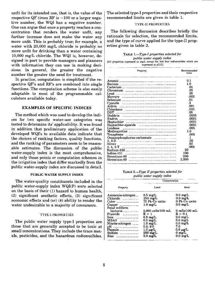
The selected type-I properties and their respective recommended limits are given in table 1.

TYPE-II PROPERTIES

The following discussion describes briefly the rationale for selection, the recommended limits, and the type of curve applied for the type-II prop­ erties given in table 2.

TABLE 1. Type-I properties selected for public water supply index

[All properties expressed in mg/L except the last four radionuclides which are expressed in pCi/L]

Property Recommended limit

Arsenic __ _ _ _Barium _ _ _ _Cadmium ___ __ __ _ .Chromium __Lead _ _Mercury _ ______Selenium _ _ _ __ _Cyanide - __ __Aldrin _ __ __ .Chlordane _ ___DOTDieldrin __ _Endrin _ _ _ _ _ _ ___ .Heptachlor ______Heptachlor-epoxide _ _ _Lindane ____ _ _ _______Methoxychlor _Toxaphene _____Organophosphorus-carbamate _ _2, 4-D _________________________ __.Silvex _ _ _ .2, 4, 5-T ___. _ ________ ___ __ __.Radium-226Iodine- 131Strontium- 90 _ _ _ _Strontium-89 __ _

_______ 0.1_______ 1.0_______ .01

.05_______ .05.-_-___ .002_______ .01

.2.__ __ .001_______ .003_______ .05.-_____ .0005_______ .0001_______ .0001_______ .0001_______ .005_______ 1.0_______ .005

.1_______ .02_______ .03_______ .002_______ 20_______ 100_______ 200. _ __ 2,000

TABLE 2. Type II properties selected for public water supply index

Concentration

Property Limit Ideal

Ammonia-nitrogen _ _ChlorideColor . _. _Copper _ _ _Fecal coliform

bacteria, _ _ _FluorideIron _ _ _MBAS ________ _ _Nitrite-nitrogen __pH ________________Phenols ___Sulfate __ _Zinc _ _

0.5 mg/L250 mg/L75 Pt-Co units1.0 mg/L

2,000 cells/100 mLR = 10.3 mg/L0.5 mg/L1.0 mg/L5.0, 9.01.0 jig/L250 mg/L5.0 mg/L

0.0 mg/L0.0 mg/L0 Pt-Co units0.0 mg/L

0 cells/100 mLR = 0.10.0 mg/L0.0 mg/L0.0 mg/L7.00.0 /_ig/LOmg/L0.0 mg/L

Ammonia. Ammonia was selected because of its effect on the efficiency of chlorination (an eco­ nomic reason) and because it is an indicator of pollution (health hazard). The recommended limit for ammonia is 0.5 mg/L and the ideal concentra­ tion is assumed to be 0.0 mg/L. Ammonia concen­ trations are expressed in terms of milligrams per liter ammonia as nitrogen (NH4-N). The linear equation determined for ammonia that is based upon the recommended limits is

QF(NH4-N)= 100-200 (mg/L NH4 -N).

Chloride. Chloride was selected because of its effect on taste and because it accelerates corrosion of distribution systems. In addition, high concen­ trations of chloride can cause water to be unfit for human consumption. The recommended limit is 250 mg/L and the ideal concentration is taken to be 0.0 mg/L. In general, the utility of a water for public supply decreases as the chloride concentra­ tion increases. The rate at which the utility de­ creases is unknown; therefore the linear form was chosen because it is the simplest expression that would express this relationship. The equation determined for chloride is

QF(C\) = 100 - QA(mg/L Cl).

Color. Color was selected because increased color can make waters esthetically undesirable; also, increased color reduces the efficiency of ion exchange resins used in water treatment facilities to remove metals. The recommended limit for color is 75 Pt-Co (platinum-cobalt) units, and the assumed ideal is 0 Pt-Co units. Esthetic accep­ tance of color in drinking water is very difficult to quantify. The author believes that the undesira- bility of a water due to color increases at a rate faster than that expressed by the linear equation; therefore the parabolic form was used. The equa­ tion for color determined from the recommended limits is

QF(color) = 100 - 0.0178(Pt-Co units)2 .

Copper. Copper was selected because it affects taste, it may accelerate corrosion, and in large doses it may cause vomiting and (or) liver-dam­ age. The recommended concentration limit ^f copper for public water supplies is l.Qjng/L. Cop­ per is essential to human health, and if the only source of this element were drinking water, the

ideal concentration would not be 0.0 mg/L; how­ ever, copper is normally consumed in adequate quantities in foodstuffs; therefore, in order to simplify the computation, the ideal concentration is taken to be 0.0 mg/L. The parabolic form of the equation was chosen for copper because it reflects the rapid degradation of drinking water due to taste by copper concentrations greater than 1.0 mg/L. The equation developed for copper was

QF(Cu)=100- 100(mg/L Cu)2 .

Fecal Coliform Bacteria. Fecal coliform bacteria were chosen because they are a more specific indicator of warm-blooded animal con­ tamination than total coliform bacteria and they are one of the major pollution indicators in use today. The recommended limit for fecal coliform bacteria is 2,000 cells/100 mL (cells per 100 milli- liter) and the ideal concentration is assumed to be 0.0 cells/100 mL. Although the absolute relation­ ship between fecal coliform bacteria and health risk from disease has not been established, it in­ tuitively seemed that the risk factor should prob­ ably be expressed in the parabolic equation. For example, the risk of becoming ill from drinking water with a fecal coliform bacteria count of 6,000 cells/100 mL is probably more than twice that re­ sulting from drinking water with a fecal coliform bacteria count of 3,000 cells/100 mL. The equa­ tion determined for fecal coliform bacteria is

QF(fecal-coli) = WQ- 0.000025fce//s 100/mL)2 .

Fluoride. As concentration of fluoride in­ creases the physiological effects increase. Lower concentrations cause mottling of teeth, chipping of teeth, and skeletal defects; extremely high con­ centrations cause illness and even death. The rec­ ommended maximum concentration of fluoride in drinking water is based on the air temperature National Academy of Sciences and National Academy of Engineering (1972) (table 3). A cer­ tain amount of fluoride in water does help to pre­ vent dental cavities; therefore, the ideal concen­ tration is set at one-tenth the recommended maximum concentration rather than zero. The fluoride value used in the equation describing its effect is the ratio ft: R = X^/X^ whe«e Xa *s the fluoride concentration in mg/L and ATm is the specific temperature recommended concentration in mg/L. This approach allows using a single ex­ pression wherein air temperature is not a vari-

TABLE 3. Recommended maximum fluoride concentrations[From National Academy ot Sciences and National Academy of Engineering, 1972]

Annual average maximum daily air temperatures

80-91 72-79 65-71 59-64 55-58 50-54

26.5-32.8 21.9-26.4 18.1-21.8 14.7-18.0 12.5-14.6 9.7-12.4

Maximum fluoride concentration

(mg/L I

1.4 1.6 1.8 2.0 2.2 2.4

able. Because the ideal value of R is not zero, a parabolic equation is used to reflect the two-sided relationship of fluoride concentrations. The equa­ tion determined for fluoride is

QF(F) =98. 8 +24. 7tR)+ 123CR )2 .

Iron. Iron affects taste, stains clothes and plumbing fixtures, and forms deposits in distribu­ tion systems. It was for these reasons, primarily aesthetic and economic, that iron was selected. The recommended limit for iron is 0.3 mg/L, and the ideal concentration is assumed to be 0.0 mg/L. The linear form was chosen because it was the simplest equation that would describe the utility decreasing as the concentration increased. The equation determined for iron is

= 100-33.3(mg/L Fe).

Methylene blue active substances. MBAS (methylene blue active substances) were chosen because of their tendency to produce undesirable aesthetic effects, to produce dispersion of insol­ uble or sorbed substances, to foam, to interfere with the removal of substances by the coagula­ tion, sedimentation, and (or) filtration processes. The recommended limit for MBAS is 0.5 mg/L, and the ideal concentration is taken to be 0.0 mg/L. The linear form was selected for the same reason it was selected for iron. The equation de­ termined for MBAS is

QF(MBAS)=WQ-2QQ(mg/L MBAS).

Nitrite-nitrogen. NO2 -N (nitrite-nitrogen) was selected because of its toxicity, particularly be­ cause it causes methemoglobinemia in infants. The recommended limit for NO2 (nitrite) is 1.0 mg/L expressed as N (nitrogen), and the ideal concentration is assumed to be 0.0 mg/L NO2 -N. As with fecal-coliform bacteria, the parabolic

form was chosen because it allows a much faster decrease in the QF than does the linear form. The equation determined for NO2 -N is

QF(NO2 N)=100-100(mg/L NO2 N)2 .

pH. pH was selected because it affects water- treatment processes and can contribute to the cor­ rosion of distribution lines and household plumb­ ing fixtures. This corrosion can add such con­ stituents as iron, copper, lead, zinc and cadmium to the water supply. The recommended limits for pH are 5.0 and 9.0, and for simplicity the ideal value is taken as 7.0. The parabolic form was cho­ sen because it is one of the simplest two-sided forms. The equation determined for pH is

QF(pH)=-l,125+35Q(pH)-25(pH)2 .

Phenols. Phenolic compounds were selected because of their effect on odor. Even though their recommended limit is quite small, they are con­ sidered a type-II property because exceeding the recommended limit does not necessarily cause a health hazard or preclude use of the water. The recommended limit for phenols is 1.0 fjig/ L(microgram per liter), and the ideal concentra­ tion is taken to be 0.0 jug/L. The linear form was selected for the same reason it was selected for iron. The equation determined for phenols is

QF(phenols) = 100 - 100(/xg/L phenols).

Sulfate. The selection of sulfate (SO4 ) was based on its taste and laxative effects. The rec­ ommended limit for sulfate is 250 mg/L, and the ideal concentration is assumed to be 0.0 mg/L. The linear form was selected for the same reason it was selected for iron. The equation determined for sulfate is

QF(SO4 )=100-0.4(mg/L SO4 ).

Zinc. Zinc was selected because of its effect on taste at higher concentrations. Zinc is essential in human metabolism, and the activities of insulin and several body enzymes are dependent upon it. The recommended limit for the maximum concen­ tration of zinc in public water supplies is 5.0 mg/L. Even though zinc is essential, the ideal concentration is set at 0.0 mg/L because adequate quantities are normally consumed in foodstuffs. The linear form was used because it expresses more closely the fact that quite high concen-

trations, 50 mg/L according to Hinman (1938), can be tolerated for protracted periods without harm. The equation determined for zinc is

QF(Zn) = 100 20(mg/L Zn).

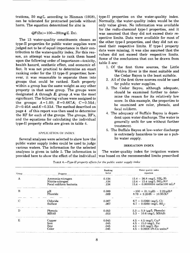
The 13 water-quality constituents chosen as type-II properties for public water supplies were judged not to be of equal importance in their con­ tribution to the water-quality index. For this rea­ son, an attempt was made to rank them based upon the following order of importance toxicity, health hazard, aesthetic effect, and economic ef­ fect. It was not practical to determine an exact ranking order for the 13 type-II properties; how­ ever, it was reasonable to separate them into groups that could be ranked. Each property within a group has the same weight as any other property in that same group. The groups were designated A through E; group A was the most significant. The following values were assigned to the groups: A = 1.00; £ = 0.667A; C = 0.50A; D = 0.40A and£=0.33A. The method described on page 4 of this report was then used to determine the RF for each of the groups. The groups, RF's, and the equations for calculating the individual type-II property effects are given in table 4.

APPLICATION OF INDEX

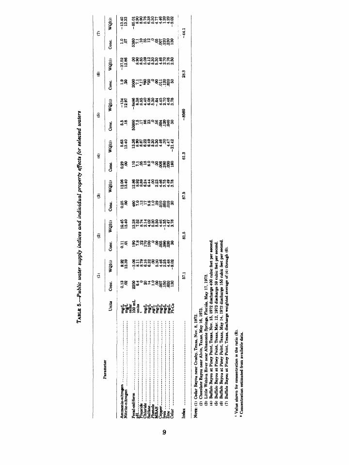
Several analyses were selected to show how the public water supply index could be used to judge various waters. The information for the selected analyses is given in table 5. The information is provided here to show the effect of the individual

type-II properties on the water-quality index. Normally, the water-quality index would be the only value given. No information was available for the radio-chemical type-I properties, and it was assumed that they did not exceed their re­ spective limits. Data were available for most of the other type-I properties, and they did not ex­ ceed their respective limits. If type-I property data were missing, it was also assumed that the values did not exceed their respective limits. Some of the conclusions that can be drawn from table 5 are:

1. Of the first three sources, the Little Wehiva River is the most suitable and the Cedar Bayou is the least suitable.

2. All of the first three sources could be used for public water supplies.

3. The Cedar Bayou, although adequate, should be examined further to deter­ mine the reason for its relatively low score. In this example, the properties to be examined are color, phenols, and fecal coliform.

4. The adequacy of Buffalo Bayou is depen­ dent upon water discharge. The water is generally unfit for use without further treatment.

5. The Buffalo Bayou at low-water discharge is extremely hazardous to use as a pub­ lic water supply.

IRRIGATION INDEX

The water-quality index for irrigation waters was based on the recommended limits prescribed

TABLE 4. Type-II property effects for the public water supply index

Group

A

B

C

D

E

Property

Ammonia-nitrogen Nitrite-nitrogen Fecal coliform bacteria

pH Fluoride

ChlorideSulfate

Phenols MBAS

Copper Iron Zinc Color

Ranking factor

0.134 .134 .134

0.089 .089

0.067 .067

0.053 .053

0.045 .045 .045 .045

Water quality index equation

13.4 - 26.8 (mg/L NH4-N) 13.4 - 13.4 (mg/L NO2-N)2 13.4 - 0.0000034 (cells/100 mL)2

-100 + 31.1(pH) - 2.22(pH)2 8.79 + 2.20CR) - 10.95CR)2

6.7 - 0.0268 (mg/L CD 6.7 - 0.0268 (mg/L SO4 )

5.3 5.3 (jU,g/L Phenols) 5.3 - 10.6 (mg/L MBAS)

4.5 - 4.5 (mg/L Cu)2 4.5 - 15.0 (mg/L Fe) 4.5 - 0.9 (mg/L Zn) 4.5 - 0.0008 (Pt-Co units)2

TABL

E 5.

~^Pu

blic

wat

er s

uppl

y in

dice

s an

d in

divi

dual

pro

pert

y ef

fect

s fo

r se

lect

ed w

ater

s

Par

amet

erU

nits

(1)

(2)

(3)

(4)

(5)

(6)

(7)

Con

e.

WQ

I(i)

Con

e.

WQ

I(i)

C

one.

W

QI(

i) C

one.

W

QI(

i) C

one.

W

Ql(

i)

Con

e.

WQ

I(i)

Con

e.

WQ

I(i)

Am

mon

ia-n

itrog

en

_________________

mg/

L

0.13

9.

92N

itri

te-n

itro

gen

__

__

__

__

__

__

__

__

__

_

mg/

L

-02

13.3

9c

ells

/Fe

cal-

colif

orm

_____________________

100

mL

22

00

-3.0

6pH

..-

. -.

-..-

-.__._

___._

..._

_ _

_ _

......__._

un

its

6.4

8.11

Fluo

ride

_ -

.--.

.-_-

_._.

_.__

____

____

____

____

.___

.._

' 0

8.79

Chl

orid

e . _

__

___._

_____________

mg/

L

20

6.16

Sulf

ate

__..

.__

__

_._

_._

..._

__

__

__

..

mg/

L

14

6.32

Phen

ols

_______________________

/tg/L

1.

0 .0

0M

BA

S

_

_ .. ..

.. .

._--

.-..

..

mg/

L .0

0 5.

30C

op

per_

__

__

__

__

__

__

__

__

__

__

__

__

m

g/L

.0

07

4.46

Iron

_

.-_

_..

_._

- _

..-

_.._

__

__

__

.__

.__

_

mg/

L

.150

2.

25Z

inc ......___....__..._

______..._

__

mg/

L

.020

4.

48C

olor

_

-.._

._-_

..._

.___

_._

____

____

__._

__._

__

Pt-C

o 13

0 -9

.02

Inde

x ___.................._________...

57.1

0.11

.0

1

190

7.8

.22

170

100 .0 .00

.005

.390

.030 30

10.4

513

.40

13.2

87.

528.

742.

144.

025.

305.

304.

46

-1.3

54.

473.

78

0.05

.0

0

400

7.0

.13 17 9.6

1.0

.29

.010

.050

.010 30

12.0

613

.40

12.8

68.

928.

896.

246.

44 .00

2.23

4.46

3.75

4.49

3.78

0.29

.0

0

110

7.1

.05 18 8.0 .0 .00

.006

.280

.030 18

0

5.63

13.4

0

13.3

68.

908.

876.

226.

495.

305.

304.

46

.30

4.47

-2

1.42

5.5

.18

5000

07.

5.1

7 86 23 .0 .56

.004

.120

.040 30

-134

12

.97

-848

6 8.

38

8.85

4.

40

6.08

5.

30-.

64

4.

45

2.70

4.

46

3.78

1.9

.20

2000 7.

1*.

17 260

220 .0 .00

.011

.120

.820 50

-37.

52

12.8

6

.00

8.90

8.85

5.09

6.12

5.30

5.30

4.46

2.70

3.76

2.50

1.0

.07

5380 7.

1.1

0 35 12 .0 .05

.007

.220

.230 13

0

-13.

40

13.3

3

-85.

01

8.90

8.

90

5.76

6.

38

5.30

4.

77

4.46

1.

20

4.29

-9.0

2

81.5

87.5

61.3

-856

028

.3

NOTE

; (1

) C

edar

Bay

ou n

ear

Cro

sby.

Tex

as,

Nov

. 8,

1972

.(2

) C

hoco

late

Bay

ou n

ear

Alv

in, T

exas

, M

ay 1

6, 1

973.

(3)

Litt

le W

ehiv

a R

iver

nea

r A

ltam

onte

Spr

ings

, Fl

orid

a, M

ay 1

7,19

73.

(4)

Buf

falo

Bay

ou a

t Pi

ney

Poin

t, T

exas

, Nov

. 15

, 19

72 d

isch

arge

400

cub

ic f

eet

per

seco

nd.

(5)

Buf

falo

Bay

ou a

t Pi

ney

Poin

t, T

exas

, M

ar.

12,1

973

disc

harg

e 59

cub

ic f

eet

per

seco

nd.

(6)

Buf

falo

Bay

ou a

t Pi

ney

Poin

t, T

exas

, M

ay 1

4, 1

973

disc

harg

e 15

5 cu

bic

feet

per

sec

ond.

(7)

Buf

falo

Bay

ou a

t Pi

ney

Poin

t, T

exas

, dis

char

ge w

eigh

ted

aver

age

of (4

) th

roug

h (6

).

1 V

alue

sho

wn

for

conc

entr

atio

n is

the

rat

io (

R).

1 C

once

ntra

tion

esti

mat

ed f

rom

ava

ilab

le d

ata.

for continuous use of water on all soil types (Na­ tional Academy of Sciences and National Academy of Engineering, 1972).

TVPE-I PROPERTIES

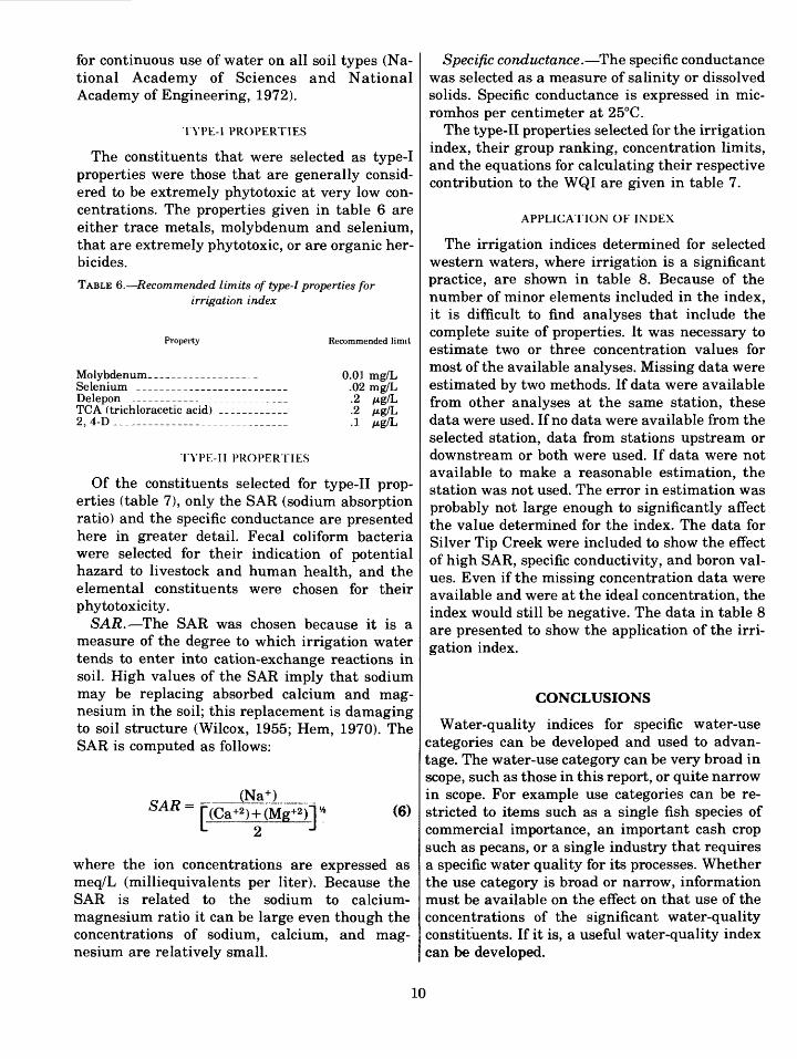
The constituents that were selected as type-I properties were those that are generally consid­ ered to be extremely phytotoxic at very low con­ centrations. The properties given in table 6 are either trace metals, molybdenum and selenium, that are extremely phytotoxic, or are organic her­ bicides.

TABLE 6. Recommended limits of type-I properties for irrigation index

Property

Molybdenum. _________Selenium ______________Delepon ________________TCA (trichloracetic acid) 2, 4-D _________._ _____

Recommended limit

0.01 mg/L .02 mg/L .2 .2 .1

TYPE-II PROPERTIES

Of the constituents selected for type-II prop­ erties (table 7), only the SAR (sodium absorption ratio) and the specific conductance are presented here in greater detail. Fecal coliform bacteria were selected for their indication of potential hazard to livestock and human health, and the elemental constituents were chosen for their phytotoxicity.

SAR. The SAR was chosen because it is a measure of the degree to which irrigation water tends to enter into cation-exchange reactions in soil. High values of the SAR imply that sodium may be replacing absorbed calcium and mag­ nesium in the soil; this replacement is damaging to soil structure (Wilcox, 1955; Hem, 1970). The SAR is computed as follows:

SAR =(Na+ )

(6)

where the ion concentrations are expressed as meq/L (milliequivalents per liter). Because the SAR is related to the sodium to calcium- magnesium ratio it can be large even though the concentrations of sodium, calcium, and mag­ nesium are relatively small.

Specific conductance. The specific conductance was selected as a measure of salinity or dissolved solids. Specific conductance is expressed in mic- romhos per centimeter at 25°C.

The type-II properties selected for the irrigation index, their group ranking, concentration limits, and the equations for calculating their respective contribution to the WQI are given in table 7.

APPLICATION OF INDEX

The irrigation indices determined for selected western waters, where irrigation is a significant practice, are shown in table 8. Because of the number of minor elements included in the index, it is difficult to find analyses that include the complete suite of properties. It was necessary to estimate two or three concentration values for most of the available analyses. Missing data were estimated by two methods. If data were available from other analyses at the same station, these data were used. If no data were available from the selected station, data from stations upstream or downstream or both were used. If data were not available to make a reasonable estimation, the station was not used. The error in estimation was probably not large enough to significantly affect the value determined for the index. The data for Silver Tip Creek were included to show the effect of high SAR, specific conductivity, and boron val­ ues. Even if the missing concentration data were available and were at the ideal concentration, the index would still be negative. The data in table 8 are presented to show the application of the irri­ gation index.

CONCLUSIONS

Water-quality indices for specific water-use categories can be developed and used to advan­ tage. The water-use category can be very broad in scope, such as those in this report, or quite narrow in scope. For example use categories can be re­ stricted to items such as a single fish species of commercial importance, an important cash crop such as pecans, or a single industry that requires a specific water quality for its processes. Whether the use category is broad or narrow, information must be available on the effect on that use of the concentrations of the significant water-quality constituents. If it is, a useful water-quality index can be developed.

10

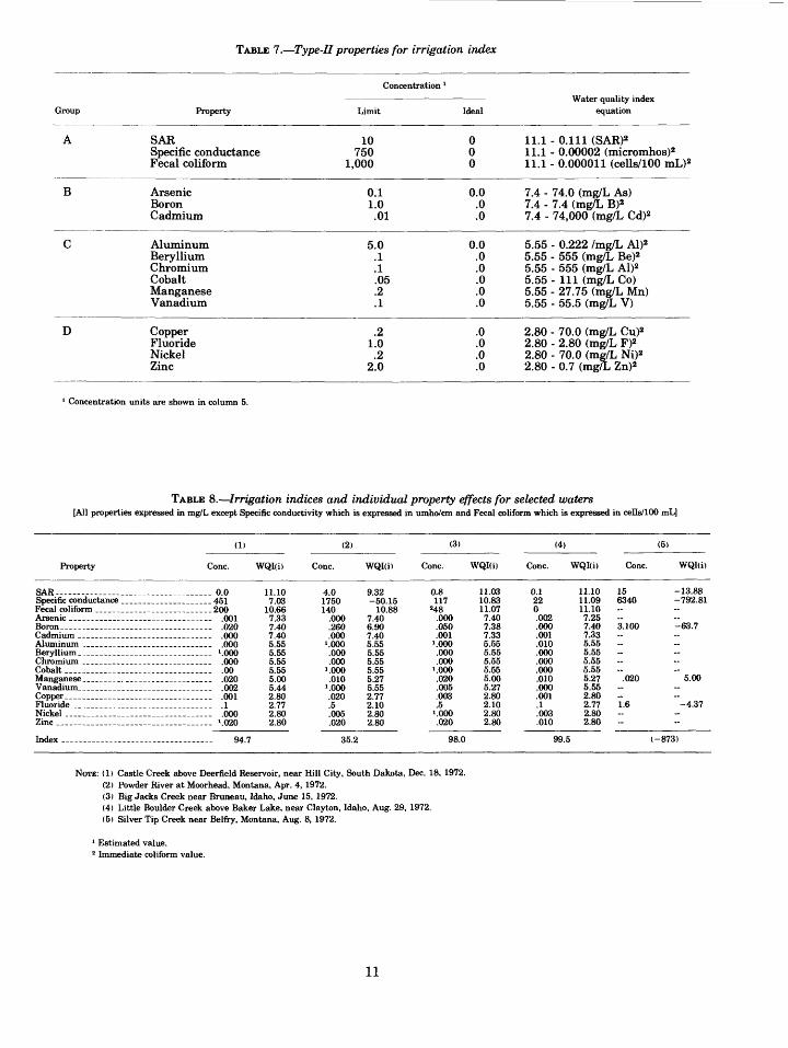
TABLE 7. Type-II properties for irrigation index

Group

A

B

C

D

Property

SAR Specific conductance Fecal coliform

Arsenic Boron Cadmium

Aluminum Beryllium Chromium Cobalt Manganese Vanadium

Copper Fluoride Nickel Zinc

Concentration *

Limit

10 750

1,000

0.1 1.0

.01

5.0 .1 .1 .05 .2 .1

.2 1.0

.2 2.0

Ideal

0 0 0

0.0 .0 .0

0.0 .0 .0 .0 .0 .0

.0

.0

.0

.0

Water quality index equation

11.1 - 0.111 (SAR)2 11.1 - 0.00002 (micromhos)2 11.1 - 0.000011 (cells/100 mL)2

7.4 - 74.0 (mg/L As) 7.4 - 7.4 (mg/L B)2 7.4 - 74,000 (mg/L Cd)2

5.55 - 0.222 /mg/L Al)2 5.55 - 555 (mg/L Be)2 5.55 - 555 (mg/L Al)2 5.55 - 111 (mg/L Co) 5.55 - 27.75 (mg/L Mn) 5.55 - 55.5 (mg/L V)

2.80 - 70.0 (mg/L Cu)2 2.80 - 2.80 (mg/L F)2 2.80 - 70.0 (mg/L Ni)2 2.80 - 0.7 (mg/L Zn)2

1 Concentration units are shown in column 5.

TABLE 8. Irrigation indices and individual property effects for selected waters[All properties expressed in mg/L except Specific conductivity which is expressed in umho/cm and Fecal coliform which is expressed in cells/100 mL]

(1) (2) (3) (4) (5)

Property Cone. WQI(i) Cone. WQI(i) Cone. WQI(i) Cone. WQI(i) Cone. WQI(i)

SAR - .Specific conductanceFecal coliform . .... _. .. ....

Cobalt. _ . . . _ __ .....

Vanadium . _ ....

Fluoride . _ . _ _ ...Nickel ................ _ .___.Zinc . . .. .

Index ... .......

..__ . 0.0 ..___. ..451. __ ......200. .___... .001.- _-_... .020

000

- .._-_- >.000nno

._._- .00._____- .020 ..___ .002.-.__...- .001. -.._ .. . .1- _ _ - .000_. ____. ».020

94.7

11.107.03

10.667.33

7 405.555.555.555.555.005.442.802.772.802.80

4.01750140

.000

.260000

'.000.000.000

'.000.010

'.000.020.5.005.020

35.5

9.32-50.15

10.887.406.907.405.555.555.555.555.275.552.772.102.802.80

I

0.8117

"48.000.050.001

'.000.000.000

'.000.020.005.003.5

'.000.020

98.0

11.0310.8311.077.407.387.335.555.555.555.555.005.272.802.102.802.80

0.1220.002.000.001.010.000.000.000.010.000.001.1.003.010

99.5

11.1011.0911.107.257.407.335.555.555.555.555.275.552.802.772.802.80

156340

3.100

..

.020

..1.6

..

-13.88-792.81 ..-63.7

5.00

..-4.37

(-873)

NOTE: (1) Castle Creek above Deerfield Reservoir, near Hill City, South Dakota, Dec. 18, 1972.(2) Powder River at Moorhead, Montana, Apr. 4, 1972.(3) Big Jacks Creek near Bruneau, Idaho, June 15, 1972.(4) Little Boulder Creek above Baker Lake, near Clayton, Idaho, Aug. 29, 1972.(5) Silver Tip Creek near Belfry, Montana, Aug. 8, 1972.

1 Estimated value.2 Immediate coliform value.

11

Most of the analytical data presently available do not contain the complete suite of properties required for application to one or more of the indi­ ces. Indices can be calculated using an incomplete suite of properties; however, the uncertainty of the index value increases with the number of missing properties. Comparing index values com­ puted from data sets having missing properties is risky at best. The comparability of two waters where different properties are missing for in­ stance, fecal coliform bacteria for one water and fluoride for the other is also risky. If one must use indices computed from incomplete suites of data, these indices should be computed from iden­ tical data sets so that they at least are directly comparable. In addition, care must be taken to inform the user of the index of the added uncer­ tainty caused by the missing data. If at all possi­ ble, the missing properties should be estimated from available data; or if the index values are to be used in management decisions, the missing data should be collected.

Certain items are not provided by the index, and any attempt to use it as a guide for these is likely to lead to erroneous conclusions. These items are:

1. The index does not provide information on the concentration and distribution of the individual water-quality properties.

2. The index represents the net effect of all the properties involved; it does not pro­ vide information on which properties have positive and which have negative effects on the index.

3. The comparison of two index numbers will not provide information as to whether one water is more amenable to treat­ ment than the other; it will indicate

only the relative use hazards in the two waters.

4. A positive index number will only indicate that on the whole the water is fit for a particular use; it will not indicate whether a given property is marginal.

The index was designed to:1. Provide directly comparable numbers

such that various waters can be judged for use in specific categories.

2. Allow for comparison of water quality changes over time.

3. Provide information that managers and other nontechnical personnel can use easily.

4. Indicate waters of "good" and "bad" water quality for specific-use categories.

REFERENCES

Brown, R. M., McClleland, N. I., Deininges, R. A., and Tozer, R., 1970, A water quality index do we dare?: Madison, Wisconsin Univ., National symposium on data and in­ strumentation for water-quality management, Proceed­ ings, p. 363-383.

Harkins, R. D., 1974, An objective water quality index: Water Pollution Control Federation Jour., v. 46, no. 3, p. 588- 591.

Hem, J. D., 1970, Study and interpretation of the chemical characteristics of natural water: U.S. Geological Survey Water-Supply Paper 1473, 363 p.

Hinman, J. J., Jr., 1938, Desirable characteristics of a munici­ pal water supply: Am. Water Works Assoc. Jour., v. 39, no. 39(3), p. 484-494.

National Academy of Sciences and National Academy of En­ gineering, 1972, Water quality criteria 1972: U.S. En­ vironmental Protection Agency, EPA R3-73-033, 594 p.

Walski, T. M., and Parker, F. L., 1974, A consumers water quality index: Am. Soc. Civil Engineers Proc., Jour. Envi­ ron. Eng. Div., v. 100, no. EE3, p. 593-611.

Wilcox, L. V., 1955, Classification and use of irrigation waters: U.S. Dept. Agriculture, Circ. 969, 19 p.

12