Water Resources Engineering 2016

PROF.P.C. SWAIN Page 1

CE 15015

WATER RESOURCES ENGINEERING

LECTURE NOTES

MODULE-IV

Department Of Civil Engineering

VSSUT, Burla

Prepared By

Dr. Prakash Chandra Swain

Professor in Civil Engineering

Veer Surendra Sai University of Technology, Burla

Branch - Civil Engineering Semester – 5th

Sem

Water Resources Engineering 2016

PROF.P.C. SWAIN Page 2

Disclaimer

This document does not claim any originality and cannot be used as a

substitute for prescribed textbooks. The information presented here

is merely a collection by Prof. P.C.Swain with the inputs of Post

Graduate students for their respective teaching assignments as an

additional tool for the teaching-learning process. Various sources as

mentioned at the reference of the document as well as freely

available materials from internet were consulted for preparing this

document. Further, this document is not intended to be used for

commercial purpose and the authors are not accountable for any

issues, legal or otherwise, arising out of use of this document. The

authors make no representations or warranties with respect to the

accuracy or completeness of the contents of this document and

specifically disclaim any implied warranties of merchantability or

fitness for a particular purpose.

Water Resources Engineering 2016

PROF.P.C. SWAIN Page 3

Course Contents

Module – IV

Flood frequency analysis: Gumbel’s method. Flood routing: Hydrologic

channel routing,

Muskingum equation, hydrologic reservoir routing: Modified Plus method,

Flood control measures.

Water Resources Engineering 2016

PROF.P.C. SWAIN Page 4

Lecture Note 1

Flood

1.1 Introduction

A flood is an overflow of water that submerges land that is usually dry. The European

Union (EU) Floods Directive defines a flood as a covering by water of land not normally covered by

water. In the sense of "flowing water", the word may also be applied to the inflow of the tide. Floods are

an area of study of the discipline hydrology and are of significant concern in agriculture, civil

engineering and public health.

Flooding may occur as an overflow of water from water bodies, such as a river, lake, or ocean, in which

the water overtops or breaks levees, resulting in some of that water escaping its usual boundaries,[3]

or it

may occur due to an accumulation of rainwater on saturated ground in an areal flood. While the size of a

lake or other body of water will vary with seasonal changes in precipitation and snow melt, these changes

in size are unlikely to be considered significant unless they flood property or drown domestic animals.

Floods can also occur in rivers when the flow rate exceeds the capacity of the river channel, particularly

at bends or meanders in the waterway. Floods often cause damage to homes and businesses if they are in

the natural flood plains of rivers. While riverine flood damage can be eliminated by moving away from

rivers and other bodies of water, people have traditionally lived and worked by rivers because the land is

usually flat and fertile and because rivers provide easy travel and access to commerce and industry.

Some floods develop slowly, while others such as flash floods, can develop in just a few minutes and

without visible signs of rain. Additionally, floods can be local, impacting a neighborhood or community,

or very large, affecting entire river basins.

In the planning and design of water resources projects, engineers and planners are often interested to

determine the magnitude and frequency of floods that will occur at the project areas. Besides the rational

method, unit hydrograph method and rainfall-runoff models method, frequency analysis is one of the

main techniques used to define the relationship between the magnitude of an event and the frequency

with which that event is exceeded. Flood Frequency Analysis is the estimation of how often a specified

event will occur. Before the estimation is carried out, analysis of the stream flow data plays a very

important role in order to obtain a probability distribution of floods. Flood frequency analysis (FFA) is

most commonly used by engineers and hydrologists worldwide and basically consists of estimating flood

peak quantities for a set of non-exceedance probabilities. Flood frequency analysis involves the fitting of

a probability model to the sample of annual flood peaks recorded over a period of observation, for a

catchment of a given region. The model parameters established can then be used to predict the extreme

events of large recurrence interval. Reliable flood frequency estimates are vital for floodplain

management; to protect the public, minimize flood related costs to government and private enterprises,

for designing and locating hydraulic structures and assessing hazards related to the development of flood

plains.

1.2 Flood Frequency Analysis

Water Resources Engineering 2016

PROF.P.C. SWAIN Page 5

Return Period: A return period, also known as a recurrence interval (sometimes repeat interval) is an estimate of

the likelihood of flood or a river discharge flow to occur. For example, a 10 year flood has a 1/10=0.1 or 10%

chance of being exceeded in any one year. This does not mean that if a flood with such a return period occurs,

then the next will occur in about ten years' time - instead, it means that, in any given year, there is a 10% chance

that it will happen, regardless of when the last similar event was.

Return Period is a statistical measurement typically based on historic data and is usually used for risk

analysis (e.g. to decide whether a project should be allowed to go forward in a zone of a certain risk, or

to design structures to withstand an event with a certain return period). Methods:

1. Weibull Method

2. Gumbell Method

3. Log Pearson Method

1.2.1 Weibull Method:

-In probability theory and statistics, it is a continuous probability distribution.

• Most commonly used method

• If ‘n’ values are distributed uniformly between 0 and 100 percent probability, then there must be n+1

intervals, n–1 between the data points and 2 at the ends.

Probability, P = m / n+1

where, m = rank

1.2.2 Gumbel’s Extreme Value Distribution Method:

• E.J. Gumbel in 1941 was consider that annual flood peaks are extreme values of floods in each of the

annual series of recorded data. Hence, floods follow the extreme value distribution.

Probability, P = 1 –

Return Period, T = 1/P

Where y = reduced variate = [1.282 (Q – ) / σ] + 0.577

e = base of Naperian Logarithm

Flood Magnitude for a given Return Period, QT = Q + KT σ

Where Frequency Factor,

T = Return Period Q = Mean σ = Standard Deviation

Water Resources Engineering 2016

PROF.P.C. SWAIN Page 6

1.2.3 Log Pearson Type III Distribution Method:

Person (1930) developed this method. In this method, it is recommended to convert the data series to

logarithms and then compute the following.

1. Compute Logarithms of flow log Q

2. Estimate Average of log Q

3. Compute Standard Deviation σ log Q

4. Compute Skew Coefficient, Cs = (N Σ (log Q – log Q)3 ) / (N-1)(N-2) (σ log Q)

3

5. QT = log Q + K (σ log Q) where K = log Pearson Frequency Factor based on Cs & Return Period

Water Resources Engineering 2016

PROF.P.C. SWAIN Page 7

Lecture Note 2

Flood routing

2.1 Introduction

Flood routing is the technique of determining the flood hydrograph at a section of a river by utilizing the data of

flood flow at one or more upstream sections. The hydrologic analysis of problems such as flood forecasting, flood

protection, reservoir design and spillway design invariably include flood routing. In these applications two broad

categories of routing can be recognized. These are:

1. Reservoir routing, and

2. Channel routing

A variety of routing methods are available and they can be broadly classified into two categories as:

1. Hydrologic routing/Lumped: Flow is calculated as a function of time alone at a particular location. Hydrologic

routing methods employ essentially the equation of continuity and flow/storage relationship.

2. Hydraulic routing/Distributed: Flow is calculated as a function of space and time throughout the system.

Hydraulic methods use continuity and momentum equation along with the equation of motion of unsteady flow

(St. Venant equations).

Hydrologic-routing methods employ essentially the equation of continuity. Hydraulic methods, on the other

hand, employ the continuity equation together with the equation of motion of unsteady.

2.2 Applications of Flood Routing

For accounting changes in flow hydrograph as a flood wave passes downstream

Flood:

•Flood Forecasting

•Flood Protection

• Flood Warning

Design:

•Water conveyance (Spillway) system

• Protective measures

•Hydro-system operation

Water Dynamics:

•Ungauged rivers

•Peak flow estimation

•River-aquifer interaction

2.3 Types of flood routing

•Lumped/hydrologic

Water Resources Engineering 2016

PROF.P.C. SWAIN Page 8

flow f(time)

Continuity equation and Flow/Storage relationship

•Distributed/hydraulic

Flow f(space, time)

Continuity and Momentum equations

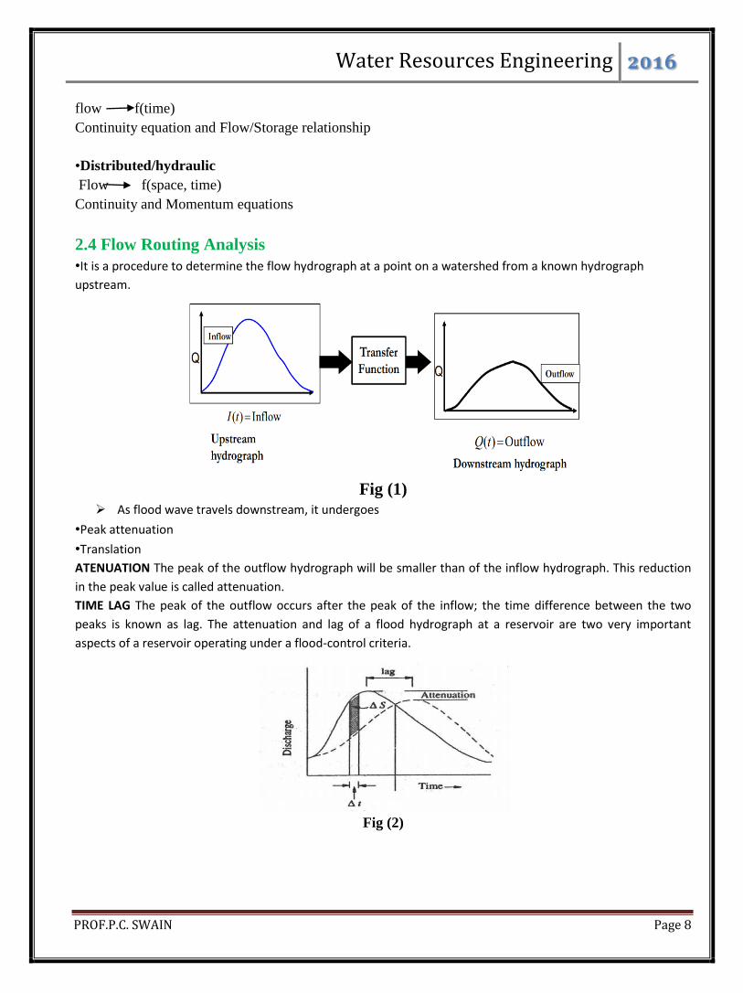
2.4 Flow Routing Analysis

•It is a procedure to determine the flow hydrograph at a point on a watershed from a known hydrograph

upstream.

Fig (1)

As flood wave travels downstream, it undergoes

•Peak attenuation

•Translation

ATENUATION The peak of the outflow hydrograph will be smaller than of the inflow hydrograph. This reduction

in the peak value is called attenuation.

TIME LAG The peak of the outflow occurs after the peak of the inflow; the time difference between the two

peaks is known as lag. The attenuation and lag of a flood hydrograph at a reservoir are two very important

aspects of a reservoir operating under a flood-control criteria.

Fig (2)

Water Resources Engineering 2016

PROF.P.C. SWAIN Page 9

2.5 Basic Equation

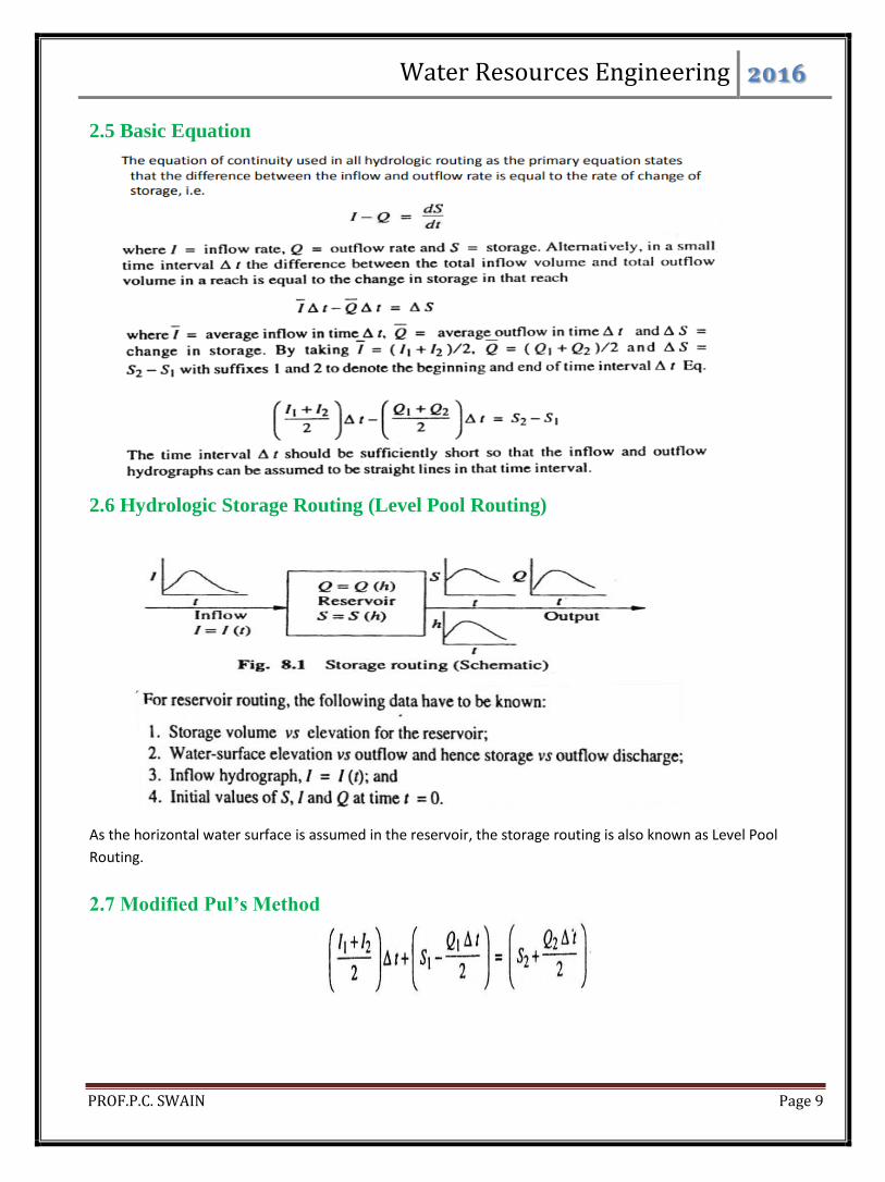
2.6 Hydrologic Storage Routing (Level Pool Routing)

As the horizontal water surface is assumed in the reservoir, the storage routing is also known as Level Pool

Routing.

2.7 Modified Pul’s Method

Water Resources Engineering 2016

PROF.P.C. SWAIN Page 10

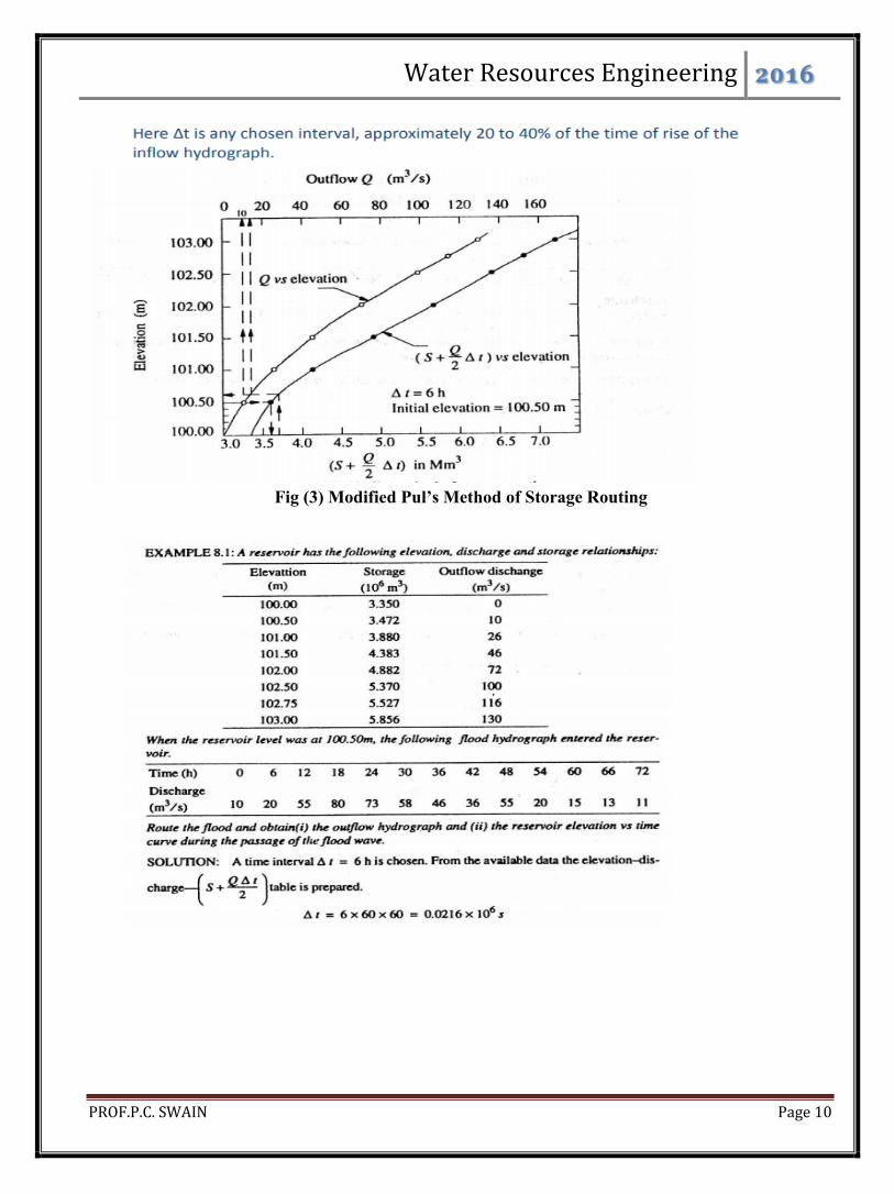
Fig (3) Modified Pul’s Method of Storage Routing

Water Resources Engineering 2016

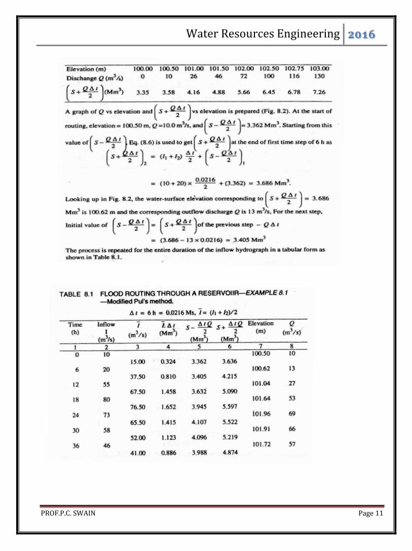
PROF.P.C. SWAIN Page 11

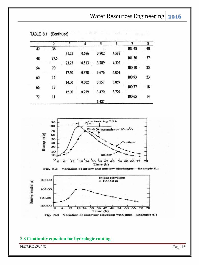
Water Resources Engineering 2016

PROF.P.C. SWAIN Page 12

2.8 Continuity equation for hydrologic routing

Water Resources Engineering 2016

PROF.P.C. SWAIN Page 13

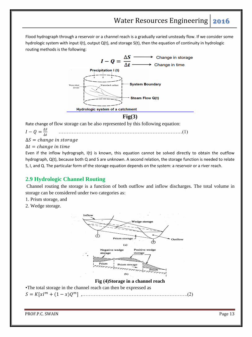
Flood hydrograph through a reservoir or a channel reach is a gradually varied unsteady flow. If we consider some

hydrologic system with input I(t), output Q(t), and storage S(t), then the equation of continuity in hydrologic

routing methods is the following:

Fig(3)

Rate change of flow storage can be also represented by this following equation:

…………………………………………………………………(1)

Even if the inflow hydrograph, I(t) is known, this equation cannot be solved directly to obtain the outflow

hydrograph, Q(t), because both Q and S are unknown. A second relation, the storage function is needed to relate

S, I, and Q. The particular form of the storage equation depends on the system: a reservoir or a river reach.

2.9 Hydrologic Channel Routing

Channel routing the storage is a function of both outflow and inflow discharges. The total volume in

storage can be considered under two categories as:

1. Prism storage, and

2. Wedge storage.

Fig (4)Storage in a channel reach

•The total storage in the channel reach can then be expressed as

,……………………………………………………….(2)

Water Resources Engineering 2016

PROF.P.C. SWAIN Page 14

Where K and x are coefficients and m = a constant exponent. It has been found that the value of m varies

from 0.6 for rectangular channels to a value of about 1.0 for natural channels.

Muskingum Equation

Using m=1, equation 2 reduces to a linear relationship for S in terms of I and Q as

……………………………………………………………….(3)

And this relationship is known as the Muskingum equation. In this the parameters x is known as

weighting factor and takes value between 0 and 0.5. When x=0,

…………………………………………………………………………………(4)

Such a storage is known as linear storage or linear reservoir.

The coefficient of K is known as Storage-time constant.

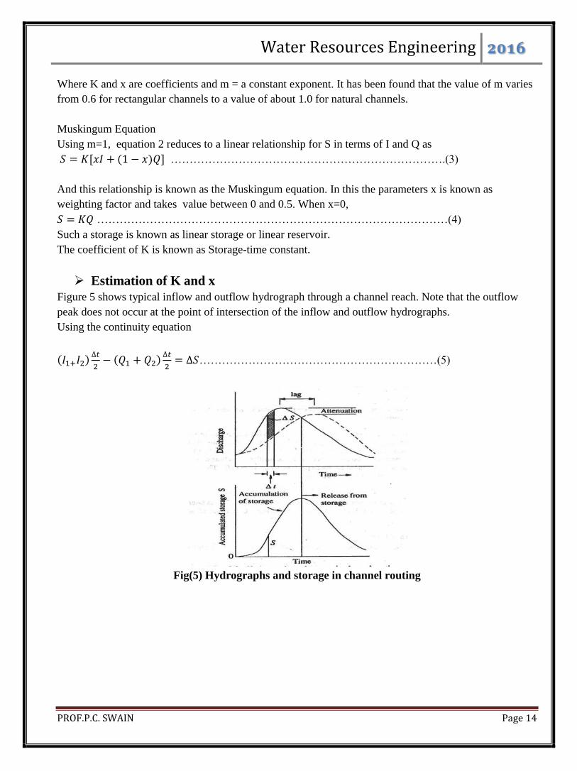
Estimation of K and x

Figure 5 shows typical inflow and outflow hydrograph through a channel reach. Note that the outflow

peak does not occur at the point of intersection of the inflow and outflow hydrographs.

Using the continuity equation

………………………………………………………(5)

Fig(5) Hydrographs and storage in channel routing

Water Resources Engineering 2016

PROF.P.C. SWAIN Page 15

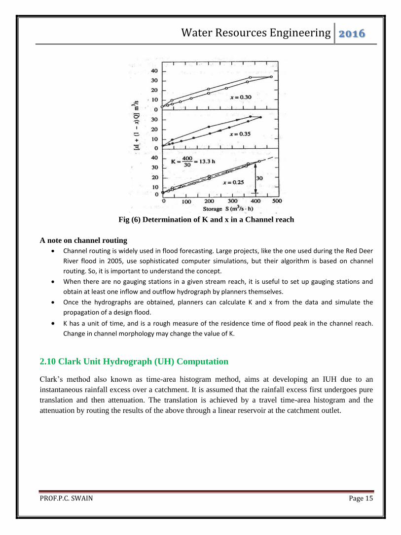
Fig (6) Determination of K and x in a Channel reach

A note on channel routing

Channel routing is widely used in flood forecasting. Large projects, like the one used during the Red Deer

River flood in 2005, use sophisticated computer simulations, but their algorithm is based on channel

routing. So, it is important to understand the concept.

When there are no gauging stations in a given stream reach, it is useful to set up gauging stations and

obtain at least one inflow and outflow hydrograph by planners themselves.

Once the hydrographs are obtained, planners can calculate K and x from the data and simulate the

propagation of a design flood.

K has a unit of time, and is a rough measure of the residence time of flood peak in the channel reach.

Change in channel morphology may change the value of K.

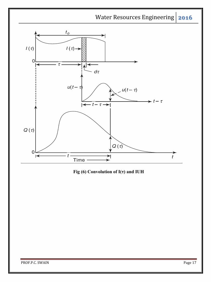
2.10 Clark Unit Hydrograph (UH) Computation

Clark’s method also known as time-area histogram method, aims at developing an IUH due to an

instantaneous rainfall excess over a catchment. It is assumed that the rainfall excess first undergoes pure

translation and then attenuation. The translation is achieved by a travel time-area histogram and the

attenuation by routing the results of the above through a linear reservoir at the catchment outlet.

Water Resources Engineering 2016

PROF.P.C. SWAIN Page 16

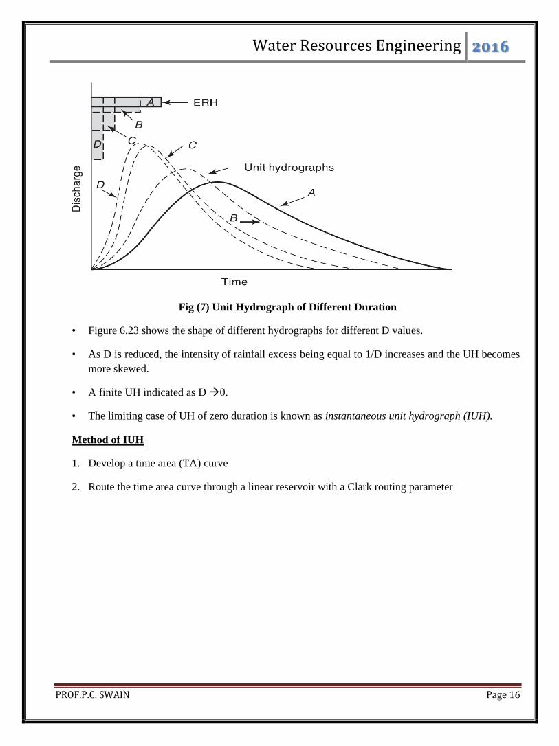
Fig (7) Unit Hydrograph of Different Duration

• Figure 6.23 shows the shape of different hydrographs for different D values.

• As D is reduced, the intensity of rainfall excess being equal to 1/D increases and the UH becomes

more skewed.

• A finite UH indicated as D 0.

• The limiting case of UH of zero duration is known as instantaneous unit hydrograph (IUH).

Method of IUH

1. Develop a time area (TA) curve

2. Route the time area curve through a linear reservoir with a Clark routing parameter

Water Resources Engineering 2016

PROF.P.C. SWAIN Page 17

Fig (6) Convolution of I(τ) and IUH

Water Resources Engineering 2016

PROF.P.C. SWAIN Page 18

REFERENCES

1. Engineering Hydrology by K. Subramanya. Tata Mc Graw Hill Publication

2. Elementary Hydrology by V.P. Singh, Prentice Hall Publication

3. Hydrology by P. Jayarami Reddy

4. Handbook of applied hydrology, V.T. Chow, Mc Graw Hill.