water resources p&m and eng. econ. microeconomics ce...
TRANSCRIPT
١
Water Resources P&M and Eng. Econ.
MicroeconomicsCE-448
٣
Microeconomics• Microeconomics (or price theory) is a branch of
economics that studies how individuals, organizations and firms make decisions to allocate limited resources, typically in markets where goods or services are being bought and sold.
• Microeconomics examines how these decisions and behaviors affect the supply and demand for goods and services, which determines prices, and how prices, in turn, determine the supply and demand of goods and services
• Microeconomics deals with the theory of behavior and markets for small agents, usually consumers, or firms that produce goods
٢
۴
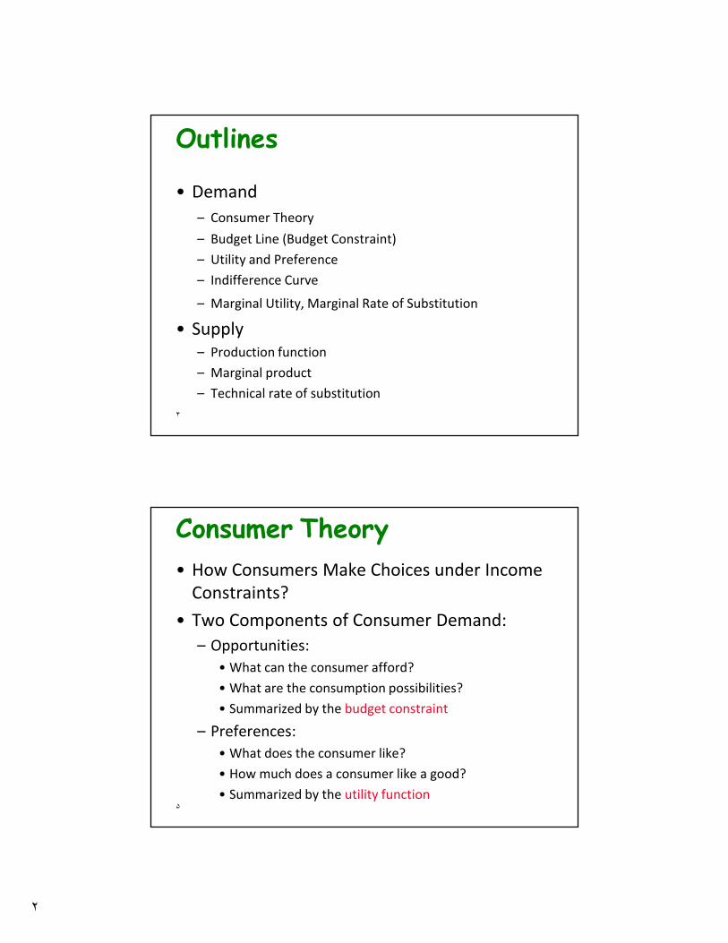
Outlines
• Demand
– Consumer Theory
– Budget Line (Budget Constraint)
– Utility and Preference
– Indifference Curve
– Marginal Utility, Marginal Rate of Substitution
• Supply– Production function
– Marginal product
– Technical rate of substitution
۵
Consumer Theory
• How Consumers Make Choices under Income
Constraints?
• Two Components of Consumer Demand:
– Opportunities:
• What can the consumer afford?
• What are the consumption possibilities?
• Summarized by the budget constraint
– Preferences:
• What does the consumer like?
• How much does a consumer like a good?
• Summarized by the utility function
٣
۶
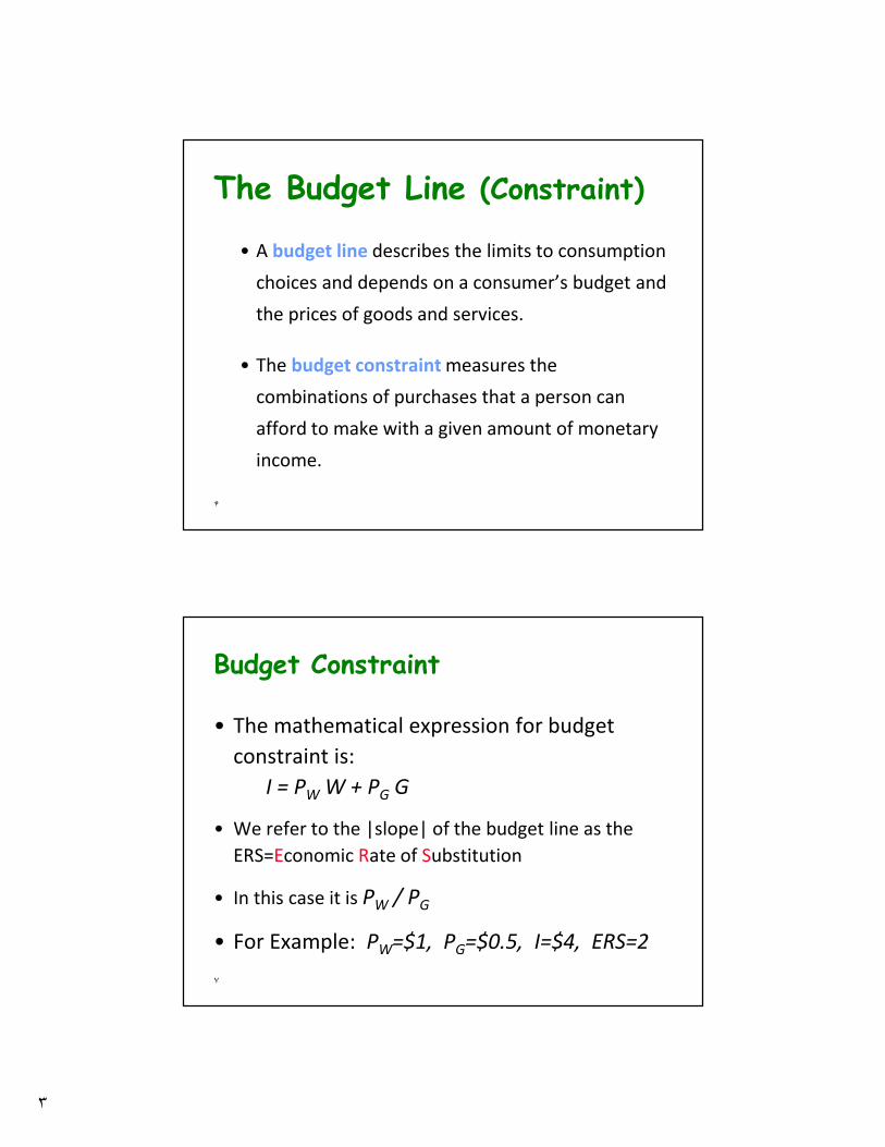
The Budget Line (Constraint)
• A budget line describes the limits to consumption
choices and depends on a consumer’s budget and
the prices of goods and services.
• The budget constraint measures the
combinations of purchases that a person can
afford to make with a given amount of monetary
income.
٧
Budget Constraint
• The mathematical expression for budget
constraint is:
I = PW W + PG G
• We refer to the |slope| of the budget line as the
ERS=Economic Rate of Substitution
• In this case it is PW / PG
• For Example: PW=$1, PG=$0.5, I=$4, ERS=2
۴
٨
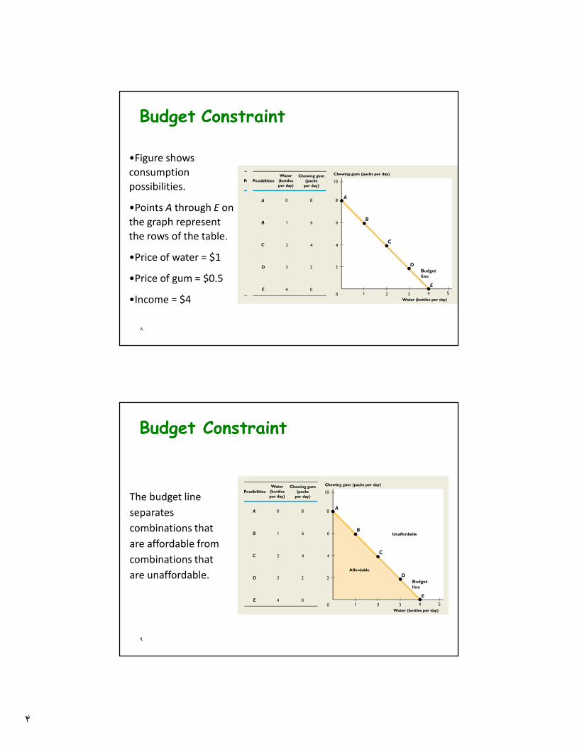
Budget Constraint
•Figure shows
consumption
possibilities.
•Points A through E on
the graph represent
the rows of the table.
•Price of water = $1
•Price of gum = $0.5
•Income = $4
٩
Budget Constraint
The budget line
separates
combinations that
are affordable from
combinations that
are unaffordable.
۵
١٠
Budget Constraint
Changes in Prices
– Shrinkage of Consumption Possibilities
• If the price of one good rises when the prices of other
goods and the budget remain the same, consumption
possibilities shrink.
– Expansion of Consumption Possibilities
• If the price of one good falls when the prices of other
goods and the budget remain the same, consumption
possibilities can expand.
١١
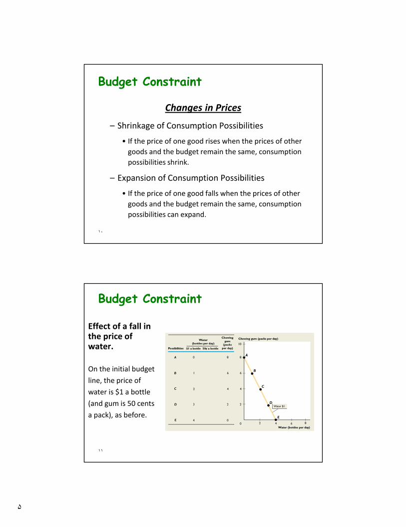
Budget Constraint
On the initial budget
line, the price of
water is $1 a bottle
(and gum is 50 cents
a pack), as before.
Effect of a fall in the price of water.
۶
١٢
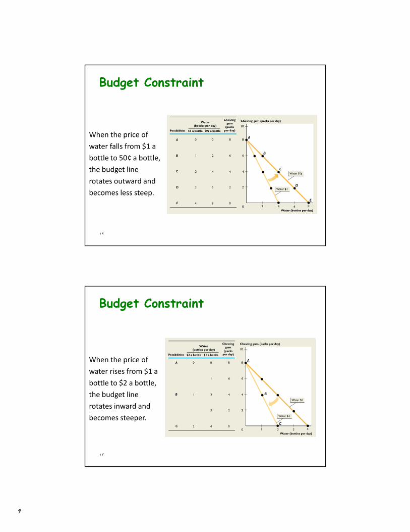
Budget Constraint
When the price of
water falls from $1 a
bottle to 50¢ a bottle,
the budget line
rotates outward and
becomes less steep.
١٣
Budget Constraint
When the price of
water rises from $1 a
bottle to $2 a bottle,
the budget line
rotates inward and
becomes steeper.
٧
١۴
Budget Constraint
• Prices and the Slope of the Budget Line
– You’ve just seen that when the price of one good
changes and the price of the other good remains
the same, the slope of the budget line changes.
– When the price of water falls, the budget line
becomes less steep.
– When the price of water rises, the budget line
becomes steeper.
– Recall that slope equals rise over run.
١۵
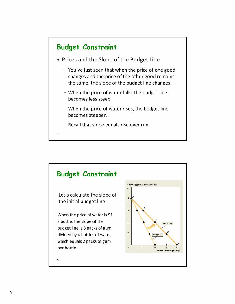
Budget Constraint
Let’s calculate the slope of
the initial budget line.
When the price of water is $1
a bottle, the slope of the
budget line is 8 packs of gum
divided by 4 bottles of water,
which equals 2 packs of gum
per bottle.
٨
١۶
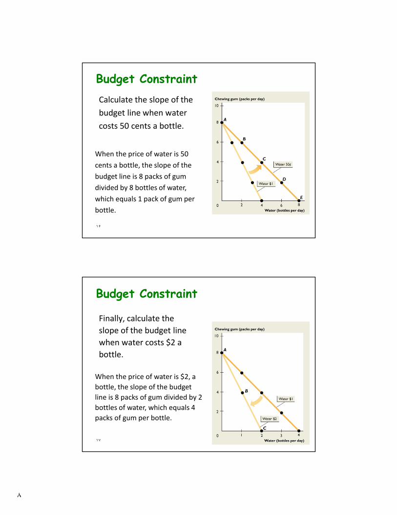
Budget Constraint
When the price of water is 50
cents a bottle, the slope of the
budget line is 8 packs of gum
divided by 8 bottles of water,
which equals 1 pack of gum per
bottle.
Calculate the slope of the
budget line when water
costs 50 cents a bottle.
١٧
Budget Constraint
When the price of water is $2, a
bottle, the slope of the budget
line is 8 packs of gum divided by 2
bottles of water, which equals 4
packs of gum per bottle.
Finally, calculate the
slope of the budget line
when water costs $2 a
bottle.
٩
١٨
Budget Constraint
– You can think of the slope of the budget line as an
opportunity cost.
– The slope tells us how many packs of gum a bottle
of water costs.
– Another name for opportunity cost is relative
price, which is the price of one good in terms of
another good = ERS.
– A relative price equals the price of one good
divided by the price of another good, and equals
the slope of the budget line.
١٩
Budget Constraint
• A Change in the Budget
– When a consumer’s budget increases,
consumption possibilities expand.
– When a consumer’s budget decreases,
consumption possibilities shrink.
١٠
٢٠
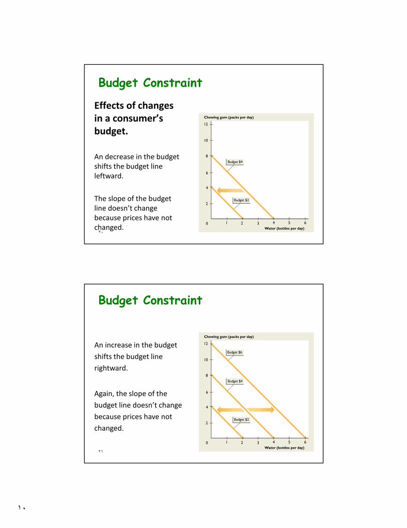
Budget Constraint
An decrease in the budget
shifts the budget line
leftward.
Effects of changes
in a consumer’s
budget.
The slope of the budget
line doesn’t change
because prices have not
changed.
٢١
Budget Constraint
An increase in the budget
shifts the budget line
rightward.
Again, the slope of the
budget line doesn’t change
because prices have not
changed.
١١
٢٢
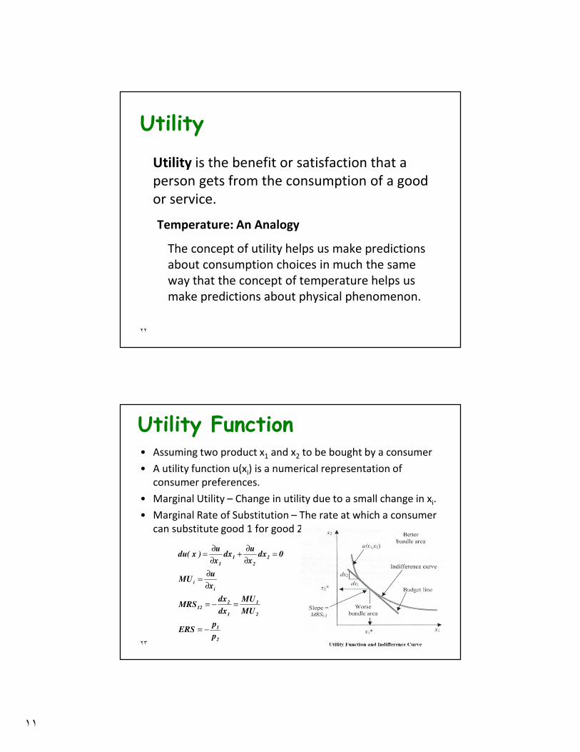
Utility
Utility is the benefit or satisfaction that a
person gets from the consumption of a good
or service.
Temperature: An Analogy
The concept of utility helps us make predictions
about consumption choices in much the same
way that the concept of temperature helps us
make predictions about physical phenomenon.
٢٣
Utility Function• Assuming two product x1 and x2 to be bought by a consumer
• A utility function u(xi) is a numerical representation of
consumer preferences.
• Marginal Utility – Change in utility due to a small change in xi.
• Marginal Rate of Substitution – The rate at which a consumer
can substitute good 1 for good 2
2
1
2
1
1
212
i
i
2
2
1
1
p
pERS
MU
MU
dx
dxMRS
x
uMU
0dxx
udx
x
u)x(du
−=
=−=
∂
∂=
=∂
∂+
∂
∂=
١٢
٢۴
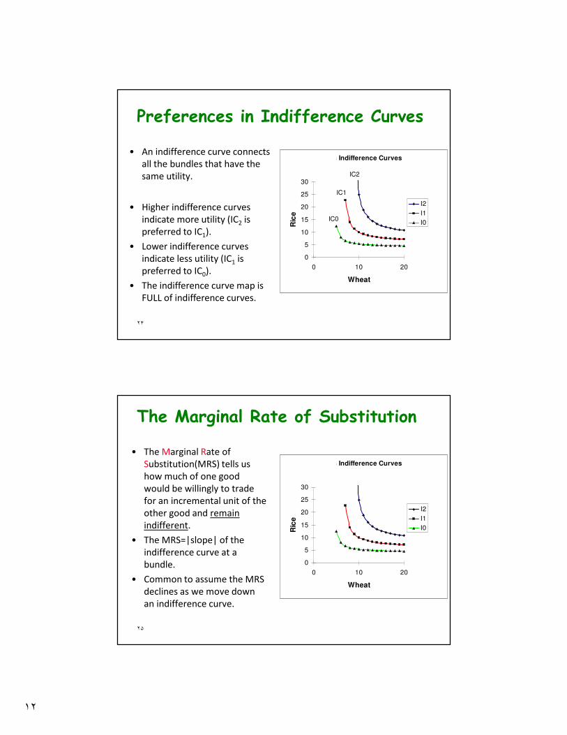
Preferences in Indifference Curves
• An indifference curve connects
all the bundles that have the
same utility.
• Higher indifference curves
indicate more utility (IC2 is
preferred to IC1).
• Lower indifference curves
indicate less utility (IC1 is
preferred to IC0).
• The indifference curve map is
FULL of indifference curves.
Li's Indifference Curves
0
5
10
15
20
25
30
0 10 20
Wheat
Ric
e
I2
I1
I0
IC2
IC1
IC0
٢۵
The Marginal Rate of Substitution
• The Marginal Rate of
Substitution(MRS) tells us
how much of one good
would be willingly to trade
for an incremental unit of the
other good and remain
indifferent.
• The MRS=|slope| of the
indifference curve at a
bundle.
• Common to assume the MRS
declines as we move down
an indifference curve.
Li's Indifference Curves
0
5
10
15
20
25
30
0 10 20
Wheat
Ric
e
I2
I1
I0
١٣
٢۶
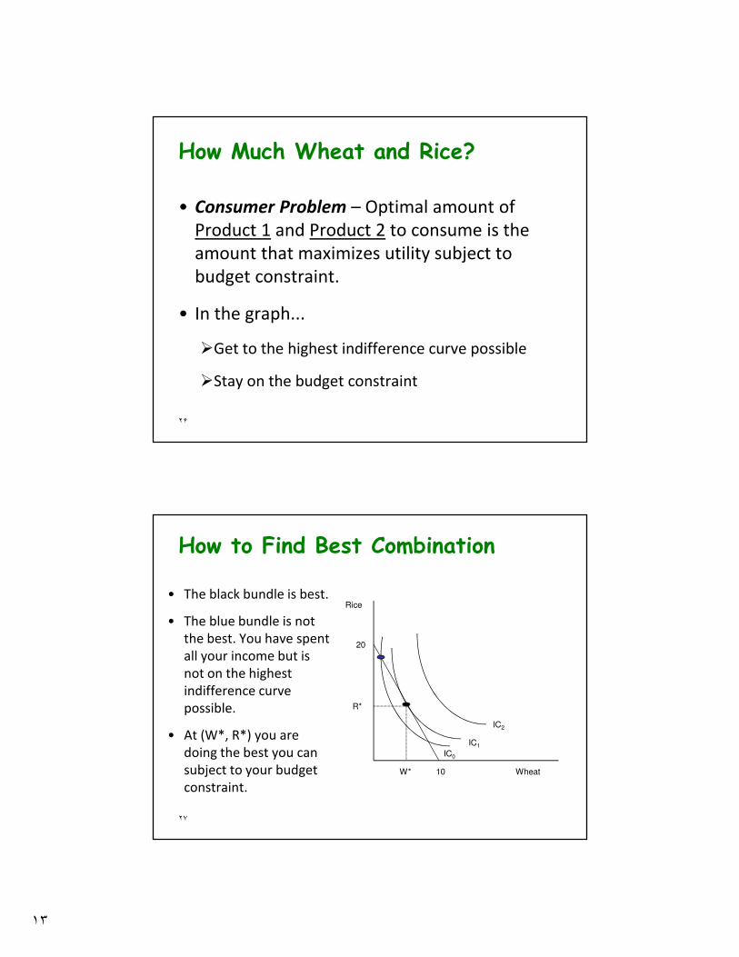
How Much Wheat and Rice?
• Consumer Problem – Optimal amount of
Product 1 and Product 2 to consume is the
amount that maximizes utility subject to
budget constraint.
• In the graph...
�Get to the highest indifference curve possible
�Stay on the budget constraint
٢٧
How to Find Best Combination
Wheat
Rice
20
10
IC0
IC1
IC2
W*
R*
• The black bundle is best.
• The blue bundle is not
the best. You have spent
all your income but is
not on the highest
indifference curve
possible.
• At (W*, R*) you are
doing the best you can
subject to your budget
constraint.
١۴
٢٨
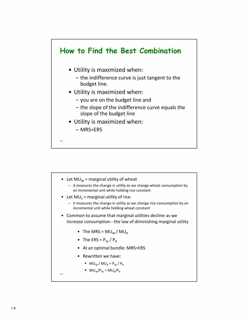
How to Find the Best Combination
• Utility is maximized when:
– the indifference curve is just tangent to the budget line.
• Utility is maximized when:
– you are on the budget line and
– the slope of the indifference curve equals the slope of the budget line
• Utility is maximized when:
– MRS=ERS
٢٩
• Let MUW = marginal utility of wheat
– it measures the change in utility as we change wheat consumption by
an incremental unit while holding rice constant
• Let MUR = marginal utility of rice
– it measures the change in utility as we change rice consumption by an
incremental unit while holding wheat constant
• Common to assume that marginal utilities decline as we
increase consumption - the law of diminishing marginal utility
• The MRS = MUW / MUR
• The ERS = PW / PR
• At an optimal bundle: MRS=ERS
• Rewritten we have:
� MUW / MUR = PW / PR
� MUW/PW = MUR/PR
١۵
٣٠
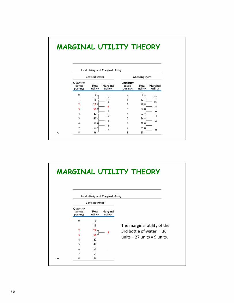
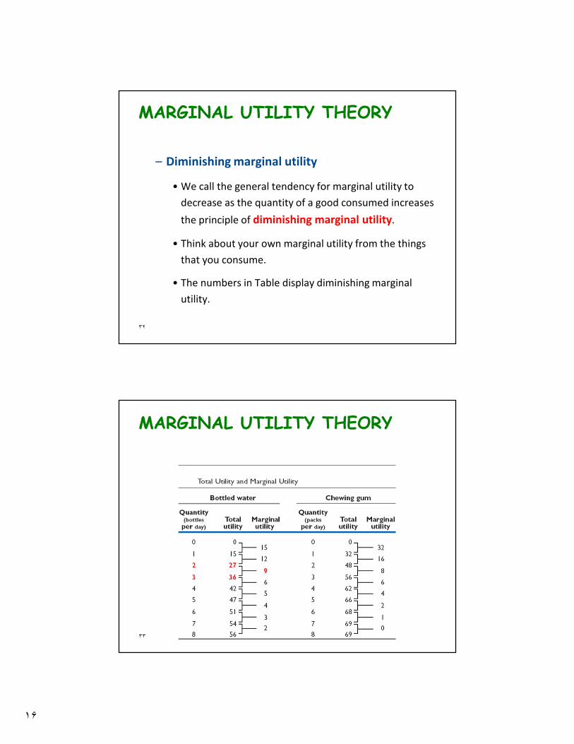
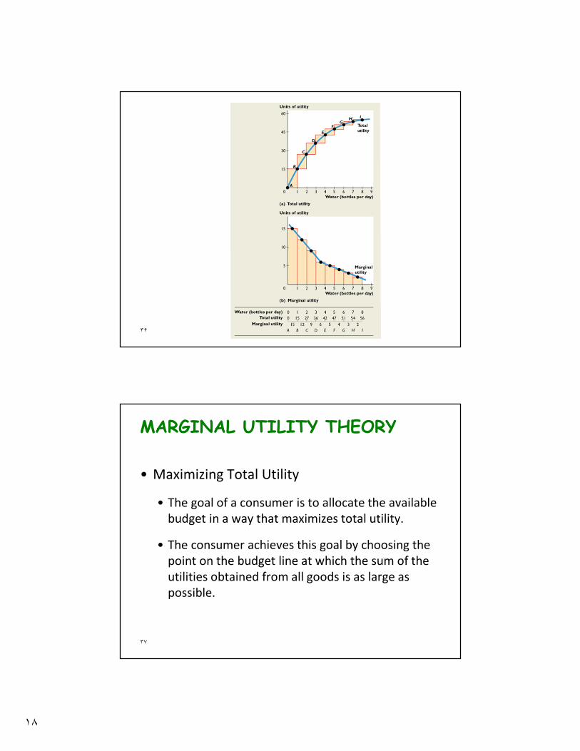
MARGINAL UTILITY THEORY
٣١
MARGINAL UTILITY THEORY
The marginal utility of the
3rd bottle of water = 36
units – 27 units = 9 units.
١۶
٣٢
– Diminishing marginal utility
• We call the general tendency for marginal utility to
decrease as the quantity of a good consumed increases
the principle of diminishing marginal utility.
• Think about your own marginal utility from the things
that you consume.
• The numbers in Table display diminishing marginal
utility.
MARGINAL UTILITY THEORY
٣٣
MARGINAL UTILITY THEORY
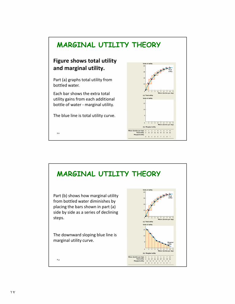
١٧
٣۴
Part (a) graphs total utility from
bottled water.
Figure shows total utility
and marginal utility.
MARGINAL UTILITY THEORY
Each bar shows the extra total
utility gains from each additional
bottle of water - marginal utility.
The blue line is total utility curve.
٣۵
Part (b) shows how marginal utility
from bottled water diminishes by
placing the bars shown in part (a)
side by side as a series of declining
steps.
The downward sloping blue line is
marginal utility curve.
MARGINAL UTILITY THEORY
١٨
٣۶
٣٧
MARGINAL UTILITY THEORY
• Maximizing Total Utility
• The goal of a consumer is to allocate the available
budget in a way that maximizes total utility.
• The consumer achieves this goal by choosing the
point on the budget line at which the sum of the
utilities obtained from all goods is as large as
possible.
١٩
٣٨
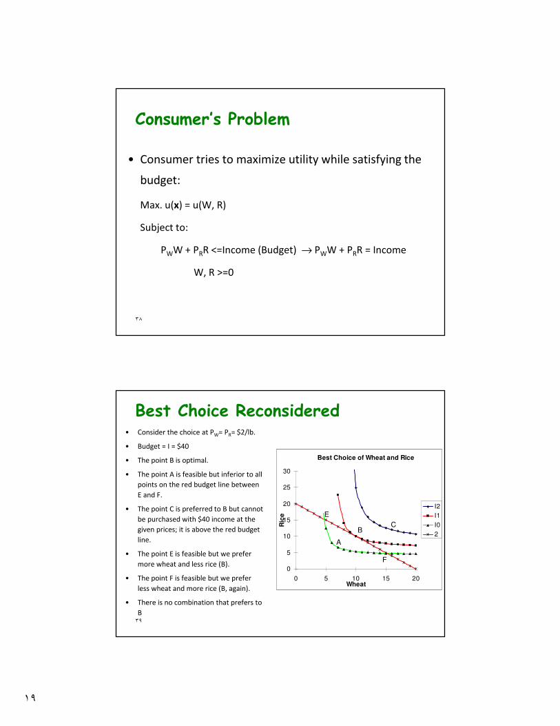
Consumer’s Problem
• Consumer tries to maximize utility while satisfying the
budget:
Max. u(x) = u(W, R)
Subject to:
PWW + PRR <=Income (Budget) → PWW + PRR = Income
W, R >=0
٣٩
Best Choice Reconsidered• Consider the choice at PW= PR= $2/lb.
• Budget = I = $40
• The point B is optimal.
• The point A is feasible but inferior to all
points on the red budget line between
E and F.
• The point C is preferred to B but cannot
be purchased with $40 income at the
given prices; it is above the red budget
line.
• The point E is feasible but we prefer
more wheat and less rice (B).
• The point F is feasible but we prefer
less wheat and more rice (B, again).
• There is no combination that prefers to
B
Li's Best Choice of Wheat and Rice
0
5
10
15
20
25
30
0 5 10 15 20Wheat
Ric
e
I2
I1
I0
2
A
E
F
BC
٢٠
۴٠
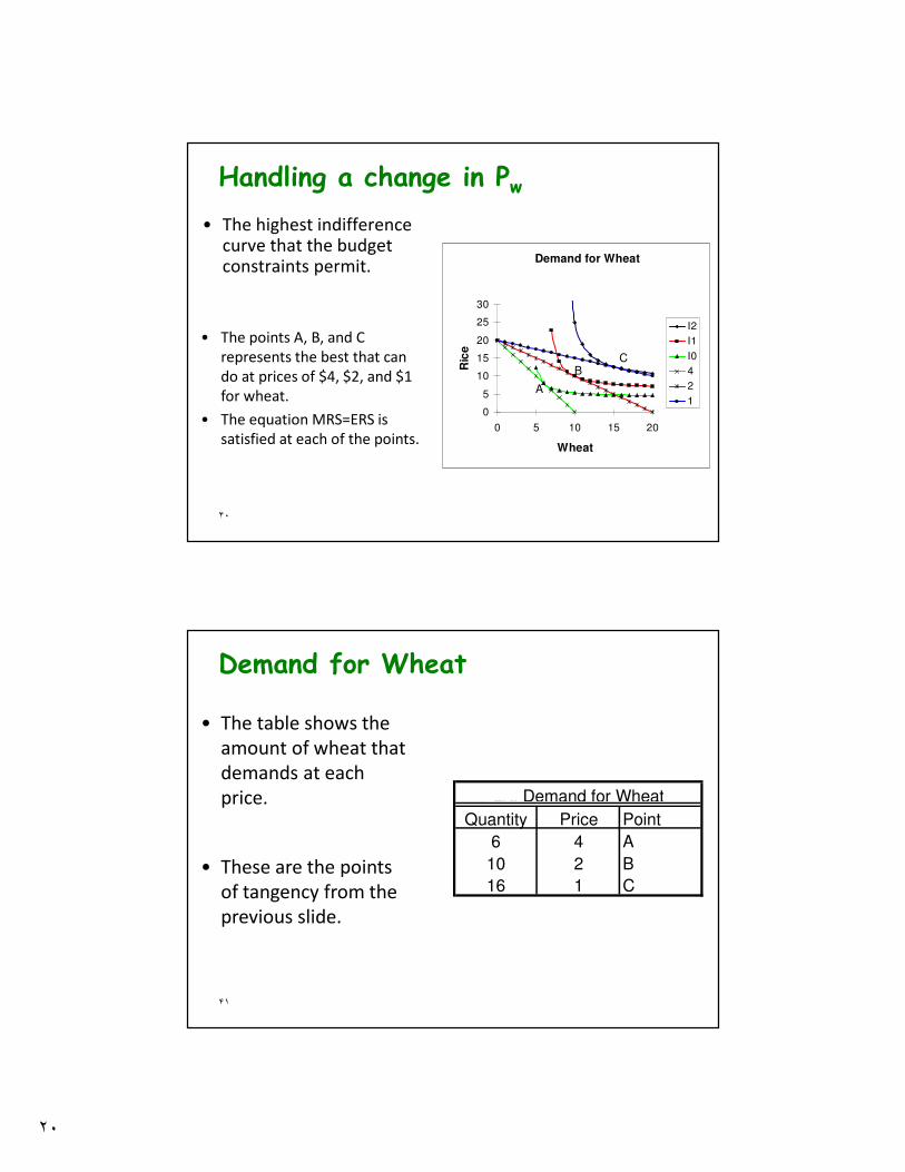
Handling a change in Pw
• The highest indifference curve that the budget constraints permit.
• The points A, B, and C
represents the best that can
do at prices of $4, $2, and $1
for wheat.
• The equation MRS=ERS is
satisfied at each of the points.
Li's Demand for Wheat
0
5
10
15
20
25
30
0 5 10 15 20
Wheat
Ric
e
I2
I1
I0
4
2
1
CB
A
۴١
Demand for Wheat
• The table shows the
amount of wheat that
demands at each
price.
• These are the points
of tangency from the
previous slide.
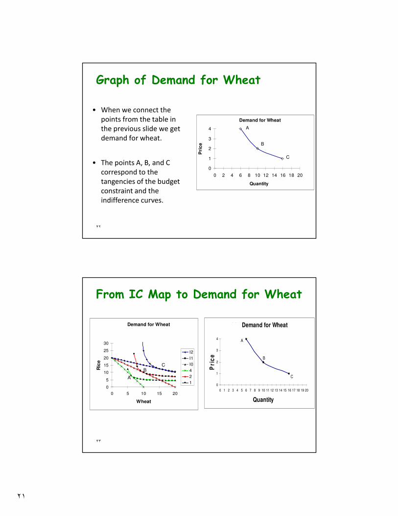
Quantity Price Point
6 4 A
10 2 B
16 1 C
Li's Demand for Wheat
٢١
۴٢
Graph of Demand for Wheat
• When we connect the
points from the table in
the previous slide we get
demand for wheat.
• The points A, B, and C
correspond to the
tangencies of the budget
constraint and the
indifference curves.
Li's Demand for Wheat
0
1
2
3
4
0 2 4 6 8 10 12 14 16 18 20
Quantity
Pri
ce
A
B
C
۴٣
Li's Demand for Wheat
0
5
10
15
20
25
30
0 5 10 15 20
Wheat
Ric
e
I2
I1
I0
4
2
1
CB
A
Li's Demand for Wheat
0
1
2
3
4
0 1 2 3 4 5 6 7 8 9 10 11 12 13 14 15 16 17 18 19 20
Quantity
Pri
ce
A
B
C
From IC Map to Demand for Wheat
٢٢
۴۴
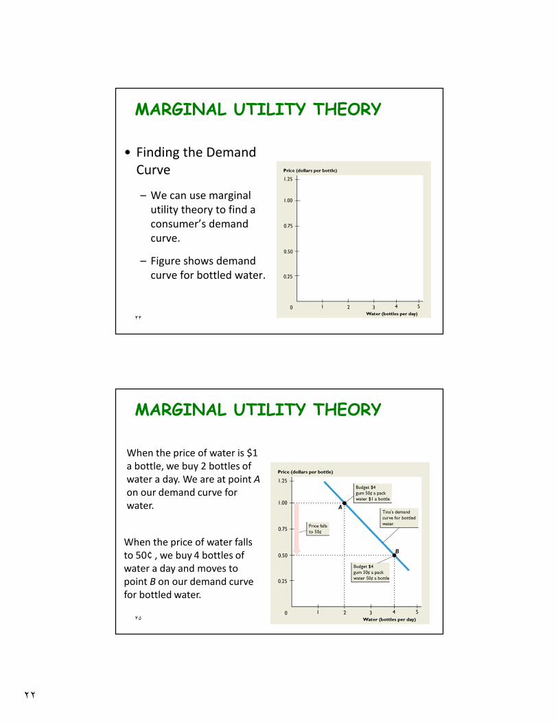
MARGINAL UTILITY THEORY
• Finding the Demand
Curve
– We can use marginal
utility theory to find a
consumer’s demand
curve.
– Figure shows demand
curve for bottled water.
۴۵
MARGINAL UTILITY THEORY
When the price of water is $1
a bottle, we buy 2 bottles of
water a day. We are at point A
on our demand curve for
water.
When the price of water falls
to 50¢ , we buy 4 bottles of
water a day and moves to
point B on our demand curve
for bottled water.
٢٣
۴۶
Supply
• Objectives:
�So far, we have studied consumer’s behavior
� In this lecture, we will study the supply side of the
market (firms…)
� It will be easier because many concepts used
when studying the firm have a clear counterpart
in the previous chapters dedicated to the
consumer
۴٧
Utility function Production function
Goods Inputs
Indifference curve Isoquant
Marginal rate of substitution
Marginal rate of technical substitution
Max utility Max profits
Min expenditure Minimize costs
٢۴
۴٨
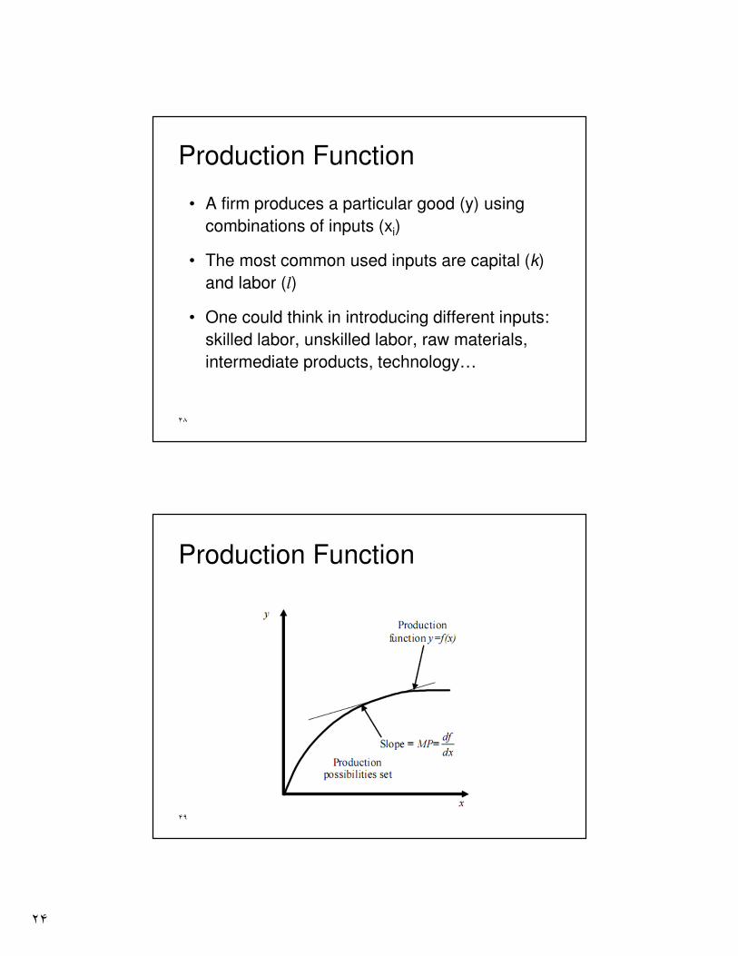
Production Function
• A firm produces a particular good (y) using
combinations of inputs (xi)
• The most common used inputs are capital (k)
and labor (l)
• One could think in introducing different inputs:
skilled labor, unskilled labor, raw materials,
intermediate products, technology…
۴٩
Production Function
٢۵
۵٠
Production Function
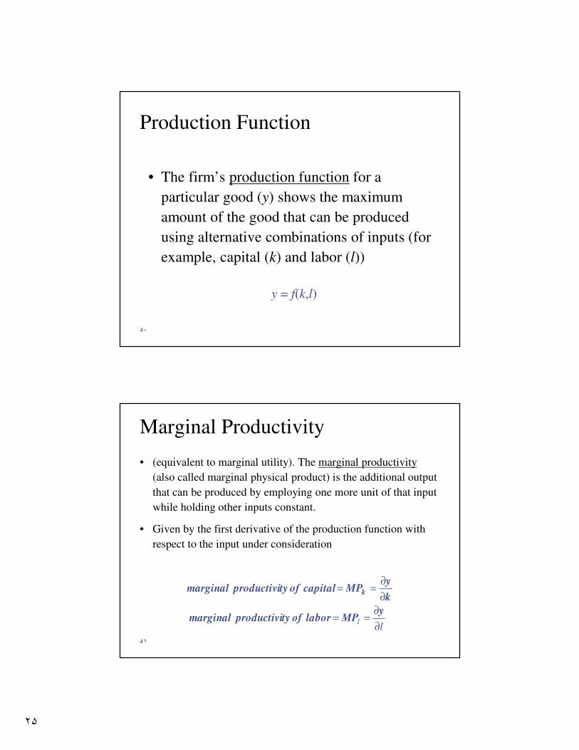
• The firm’s production function for a
particular good (y) shows the maximum
amount of the good that can be produced
using alternative combinations of inputs (for
example, capital (k) and labor (l))
y = f(k,l)
۵١
Marginal Productivity
• (equivalent to marginal utility). The marginal productivity
(also called marginal physical product) is the additional output
that can be produced by employing one more unit of that input
while holding other inputs constant.
• Given by the first derivative of the production function with
respect to the input under consideration
k
yMP capital ofty productivi marginal k
∂
∂==
ll
∂
∂==
yMP labor ofty productivi marginal
٢۶
۵٢
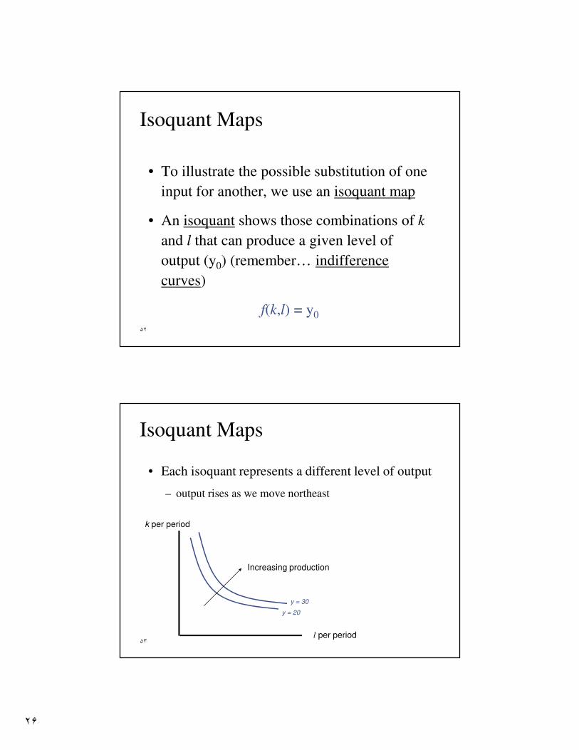
Isoquant Maps
• To illustrate the possible substitution of one
input for another, we use an isoquant map
• An isoquant shows those combinations of k
and l that can produce a given level of
output (y0) (remember… indifference
curves)
f(k,l) = y0
۵٣
Isoquant Maps
l per period
k per period
• Each isoquant represents a different level of output
– output rises as we move northeast
y = 30
y = 20
Increasing production
٢٧
۵۴
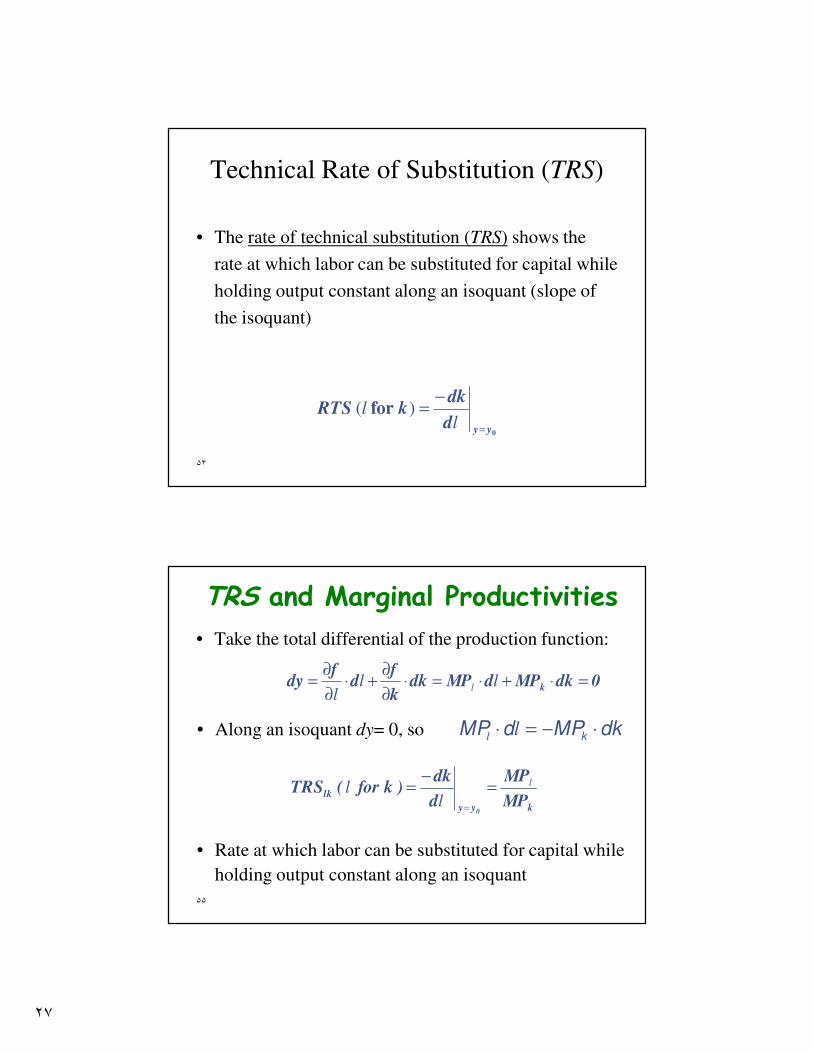
Technical Rate of Substitution (TRS)
• The rate of technical substitution (TRS) shows the
rate at which labor can be substituted for capital while
holding output constant along an isoquant (slope of
the isoquant)
0
for
yyd
dkkRTS
=
−=
ll )(
۵۵
TRS and Marginal Productivities
• Take the total differential of the production function:
0dkMPdMPdkk
fd
fdy k =⋅+⋅=⋅
∂
∂+⋅
∂
∂= ll
ll
• Along an isoquant dy= 0, so dkMPdMP k ⋅−=⋅ ll
kyy
lkMP
MP
d
dk)k for ( TRS
0
l
ll =
−=
=
• Rate at which labor can be substituted for capital while
holding output constant along an isoquant
٢٨
۵۶
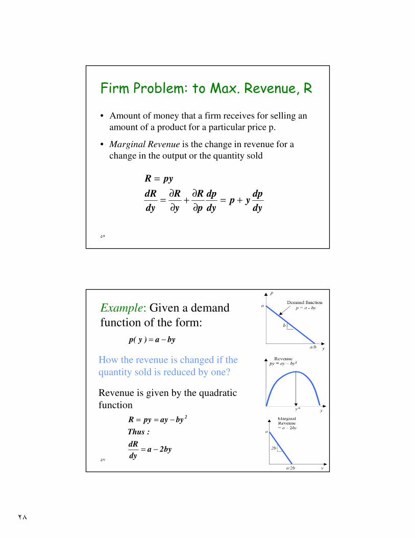
Firm Problem: to Max. Revenue, R
• Amount of money that a firm receives for selling an
amount of a product for a particular price p.
• Marginal Revenue is the change in revenue for a
change in the output or the quantity sold
dy
dpyp
dy
dp
p
R
y
R
dy
dR
pyR
+=∂
∂+
∂
∂=
=
۵٧
Example: Given a demand
function of the form:
bya)y(p −=
How the revenue is changed if the
quantity sold is reduced by one?
Revenue is given by the quadratic
function
by2ady
dR
:Thus
byaypyR 2
−=
−==