water supply options for the growing megacity of yangon
TRANSCRIPT
Institut für Wasserwirtschaft, Hydrologie
und landwirtschaftlichen Wasserbau
Master Thesis
Water supply options for the growing megacity of Yangon -
scenarios with the WEAP model
Water Resources and Environmental Management (WATENV)
Leibniz University Hannover
Zaw Win Aung
Matr.-Nr. 2919270
Examiner:
Dr.-Ing. Jörg Dietrich, Dr.-Ing. Sven van der Heijden
Advisors:
Dr.-Ing. Jörg Dietrich, Dr.-Ing. Sven van der Heijden
September 2014

Institut für Wasserwirtschaft, Hydrologie
und landwirtschaftlichen Wasserbau
Prof. Dr.-Ing. U. Haberlandt (GL) Appelstr. 9A, 30167 Hannover
Dr.-Ing. J. Dietrich Tel: +49 (0)511 762 2237 Fax: +49 (0)511 762 3731 E-Mail: [email protected]
Web: www.iww.uni-hannover.de
_________________________________________________________________________________________________________________________________________________________________________
II
Master Thesis for
Zaw Win Aung, Matr.-No. 2919270
“Water supply options for the growing megacity of Yangon - scenarios with the
WEAP model”
Integrated water resources planning models can simulate the water balance and the impact
of different water uses on the water balance. Different management schemes can be imple-
mented and compared. WEAP (Water Evaluation And Planning System) is a model often
used in developing countries, which is particularly strong in the development of IWRM
schemes for a sustainable water use in the region or catchment.
In this study, a WEAP model for the water supply system of the city of Yangon, Myanmar,
should be developed, which will be applied to analyze different options for future water sup-
ply under growing water demand.
The following points need to be addressed in the thesis:
1) Literature research: models of water availability and demand for large cities in rapidly
developing urban regions, applications of the WEAP model in developing countries,
esp. in monsoon regions
2) Overview of the Yangon water supply system and water uses
3) Development of a WEAP model for water supply of Yangon
4) Simulation of status quo and future scenarios including the following aspects:
Evaluation of WEAP for today’s supply system and demand
Estimation of future demand under population growth and development
Different sources and techniques (e.g. used or brackish water) for extension
of the current system in a sustainable manner
5) Evaluation of the scenarios
How could the future development influence water flows?
How will the reliability of the supply system develop?
Recommendation for long term planning of the system from the water availa-
bility point of view

Water supply options for the growing megacity of Yangon - scenarios with the WEAP model
III
The ArcGIS software is available for this thesis. The student needs to acquire a license of the
WEAP model, which is free for students from developing countries.
The completed work should give a well sorted overview over the topic using diagrams and
tables. One electronic and two hardcopy versions of the work have to be submitted. The stu-
dent has to present the results in a talk of 20 minutes duration plus discussion.
Date of issue:
Date of start:
Date of end:
Advisors: Dr.-Ing. Jörg Dietrich, Dr.-Ing. Sven van der Heijden
Examiner 1: Dr.-Ing. Jörg Dietrich
Examiner 2: Dr.-Ing. Sven van der Heijden
Hannover, 01.04.2014

Water supply options for the growing megacity of Yangon - scenarios with the WEAP model
IV
Declaration
I declare that I have written this Master’s Thesis independently. No other that the given
sources and resources were used. The quotations or the consulted materials have been identi-
fied as such.
[I declare that this research paper for the degree of Master of Water Resources and Environ-
mental Management, Faculty of Civil Engineering at Leibniz University Hannover hereby
submitted has not been submitted by me or anyone else for a degree at this or any other uni-
versity. That it is my own work and that materials consulted have been properly acknowl-
edged.]
City, Date: …………………………………… Signature: ……………………………………..

Water supply options for the growing megacity of Yangon - scenarios with the WEAP model
V
Acknowledgements
First and foremost, I would like to thank my advisors, Dr. -Ing. Jörg Dietrich and Dr. -
Ing. Sven van der Heijden, for providing a master thesis topic, which is related to Yangon
City Water Supply System, and for accepting me to advise and supervise my thesis. I am
grateful for their support, providing me all the knowledge and explanations that I need to
know in my thesis.
Secondly, I would like to express my special thanks to Chief Engineer, Head of De-
partment, Engineering Department (Water & Sanitation), Yangon City Development Commit-
tee, for allowing me to work on Master thesis related with water supply management of Yan-
gon City. Additionally, I sincerely thank all engineers and employees from this department
providing me all data and documents I needed and for coordinating throughout my research.
Moreover, I also want to thank JICA expert and JICA master plan team for Water & Sanita-
tion Department (YCDC) for providing the data I requested during my research.
Additionally, I am also greatly thankful to Department of City Planning and Land
Administration (YCDC), Department of Meteorology and Hydrology (Myanmar), Ministry of Agri-
culture and Irrigation and other local and global institutions for providing the data, information
and technical supports concerning with this study.
Finally, I would like to express my gratitude to DAAD scholarship program for mak-
ing me possible to study in Germany, and I would like to give the most honest thanks to my
parents, my sisters and my friends for encouraging me to continue my studies and supporting
me throughout my studies.
Water supply options for the growing megacity of Yangon - scenarios with the WEAP model
VI
Abstract
Integrated Water Resources Management approach using software tools can provide effective
results for water supply and demand analysis. This study used Water Evaluation And Planning System
(WEAP) modelling software as a tool to develop a model for Yangon City Water Supply System
(YCWSS) and this model was applied to analyse the situation of current system and the impacts of
various external alternatives and management options mainly focusing on the water demand coverage
of Yangon City. To develop this model, Hydrological and meteorological data and water supply-
demand data were obtained from Department of Meteorology and Hydrology (Myanmar), Ministry of
Agriculture and Irrigation, and Engineering Department (Water & Sanitation), Yangon City Develop-
ment Committee. Moreover, Rainfall-runoff (simplified coefficient) method and Specify yearly de-
mand and monthly variation method were used to simulate the water supply and demand. In this mod-
el, Reference Scenario was created to represent the current water supply system. For scenarios analy-
sis, other scenarios were explored from the reference scenario, which are external driven scenarios for
socioeconomic change and climate change, and management scenarios for both demand-side and sup-
ply-side. Three scenarios for socioeconomic change were built to analyse the effect of high population
growth, low population growth, and higher living standards, and a climate change scenario using a
global climate model data was constructed. Four scenarios for management strategies were developed
to analyse the effect of management practise on both demand and supply sides such as water-pricing
policy, sustainable water source, non-revenue water control, and alternative supply source. The results
of Reference Scenario were verified using observed volume of reservoirs for supply sources and ob-
served demand coverage of Yangon City for demand site, and these results showed that the future
unmet demand of Yangon City under this scenario will be 202 MGD with demand coverage 33% in
2040. According to the results of other scenarios analysis, high population growth with higher living
standards scenario will face the worst situation in Yangon City declining 11% demand coverage with
the unmet demand amount 461 MGD in 2040. However, implementation of four management strate-
gies in Yangon City under this worst situation can achieve 100% demand coverage starting from 2030.
Even implementing three management strategies except extending alternative supply sources under
Reference Scenario demonstrated that the demand coverage in Yangon City can get about 80% in
2040 and the unmet demand will be 50 MGD. According to these results, the two proposed projects in
YCWSS with 240 MGD capacity and 180 MGD capacity should be revised concerning with capacities
and project periods. As a result, this study can formulate the strategic development options for
YCWSS to adapt under future alternatives, and this WEAP model can assist water managers and local
authorities of Yangon City in decision making for the improvement of YCWSS.
Keywords: Socioeconomic change; Climate change; Modelling; Scenarios analysis; Management
strategies; Yangon City Water Supply System

Water supply options for the growing megacity of Yangon - scenarios with the WEAP model
VII
TABLE OF CONTENTS
DECLARATION ................................................................................................................................................. IV
ACKNOWLEDGEMENTS .................................................................................................................................. V
ABSTRACT ......................................................................................................................................................... VI
LIST OF FIGURES ............................................................................................................................................ IX
LIST OF TABLES .............................................................................................................................................. XI
LISTS OF ABBREVIATIONS ........................................................................................................................ XII
LISTS OF UNIT CONVERSIONS ................................................................................................................. XIII
1 INTRODUCTION ....................................................................................................................................... 1
1.1 BACKGROUND ........................................................................................................................................... 2 1.2 STUDY PROBLEM ....................................................................................................................................... 5
1.3 STUDY OBJECTIVE ..................................................................................................................................... 6 1.4 STUDY METHODOLOGY .............................................................................................................................. 6 1.5 STRUCTURE OF THE THESIS ....................................................................................................................... 7
2 LITERATURE REVIEW ........................................................................................................................... 8
2.1 WATER RESOURCES MANAGEMENT MODELS ........................................................................................... 8 2.2 WEAP MODEL ......................................................................................................................................... 12
2.3 APPLICATIONS OF WEAP MODEL ............................................................................................................ 16
3 YANGON CITY WATER SUPPLY SYSTEM ....................................................................................... 19
3.1 OVERVIEW OF STUDY AREA .................................................................................................................... 19
3.1.1 Natural Situation ........................................................................................................................... 19 Location .................................................................................................................................................... 19 3.1.1.1
Area .......................................................................................................................................................... 20 3.1.1.2
Geography ................................................................................................................................................ 21 3.1.1.3
Climatology .............................................................................................................................................. 21 3.1.1.4
3.1.2 Hydrological Situation .................................................................................................................. 25 3.1.3 Social-economic situation ............................................................................................................. 25
Population ................................................................................................................................................. 25 3.1.3.1
Urbanization ............................................................................................................................................. 26 3.1.3.2
Present Land Use ...................................................................................................................................... 29 3.1.3.3
Industrialization ........................................................................................................................................ 29 3.1.3.4
Health ....................................................................................................................................................... 30 3.1.3.5
3.2 STUDY ORGANIZATION DESCRIPTION...................................................................................................... 30 3.2.1 Yangon City Development Committee (YCDC) ............................................................................. 30
3.2.2 Engineering Department (Water & Sanitation) ............................................................................ 32 3.3 HISTORY AND STATUS QUO OF WATER SUPPLY SYSTEM ......................................................................... 33
3.3.1 Past Water Supply System ............................................................................................................. 33 3.3.2 Present Water Supply System ........................................................................................................ 34
Water Supply Sources............................................................................................................................... 34 3.3.2.1
Demand sites ............................................................................................................................................ 38 3.3.2.2
Water Supply Service Condition .............................................................................................................. 39 3.3.2.3
Problems in YCWSS ................................................................................................................................ 41 3.3.2.4
Consumer Survey ..................................................................................................................................... 41 3.3.2.5
Service level target for future ................................................................................................................... 43 3.3.2.6
4 DEVELOPMENT OF WEAP MODEL FOR YCWSS .......................................................................... 45

Water supply options for the growing megacity of Yangon - scenarios with the WEAP model
VIII
4.1 STUDY DEFINITION .................................................................................................................................. 48
4.2 DATA ENTRY IN THE CURRENT ACCOUNTS ............................................................................................... 49 4.2.1 Demand Sites and Catchments ...................................................................................................... 50
Demand sites ............................................................................................................................................ 50 4.2.1.1
Catchments ............................................................................................................................................... 52 4.2.1.2
4.2.2 Supply and Resources.................................................................................................................... 55 Local reservoirs ........................................................................................................................................ 55 4.2.2.1
Groundwater ............................................................................................................................................. 59 4.2.2.2
Rivers........................................................................................................................................................ 60 4.2.2.3
Transmission links .................................................................................................................................... 61 4.2.2.4
Runoff and infiltration .............................................................................................................................. 62 4.2.2.5
Return flow ............................................................................................................................................... 62 4.2.2.6
4.2.3 Others ............................................................................................................................................ 63 Waste water treatment plant ..................................................................................................................... 63 4.2.3.1
Key Assumption and Other Assumptions ................................................................................................. 63 4.2.3.2
5 CREATION OF SCENARIOS IN YCWSS-WEAP MODEL ............................................................... 64
5.1 REFERENCE SCENARIO ............................................................................................................................ 65 5.2 OTHER SCENARIOS .................................................................................................................................. 67
5.2.1 External driven scenarios .............................................................................................................. 68 Socioeconomic Change Scenarios ............................................................................................................ 68 5.2.1.1
Climate change Scenario .......................................................................................................................... 71 5.2.1.2
5.2.2 Management Scenarios ................................................................................................................. 72 Demand-side Management (DSM) Scenarios ........................................................................................... 72 5.2.2.1
Supply-side Management (SSM) scenarios .............................................................................................. 74 5.2.2.2
6 SIMULATION AND EVALUATION OF SCENARIOS ....................................................................... 76
6.1 EVALUATION OF THE CURRENT YCWSS IN REFERENCE SCENARIO ........................................................ 76 6.1.1 Estimation of Future Demand in YCWSS ...................................................................................... 79
6.1.2 Prediction for Extension of YCWSS .............................................................................................. 80 6.2 IMPACTS OF EXTERNAL DRIVEN SCENARIOS ............................................................................................ 84
6.2.1 High Population Growth - HPG Scenario .................................................................................... 85 6.2.2 Low Population Growth - LPG Scenario ...................................................................................... 85 6.2.3 Higher Living Standards - HLS Scenario ...................................................................................... 86
6.2.4 Climate Change Scenario - CC Scenario ...................................................................................... 86 6.3 ADVANTAGES OF MANAGEMENT SCENARIOS .......................................................................................... 87
6.3.1 1st DSM - Water Pricing Policy (WPP) Scenario .......................................................................... 88
6.3.2 2nd
DSM - Sustainable Water Source (SWS) Scenario .................................................................. 88 6.3.3 1
st SSM – NRW Control (NRWC) Scenario ................................................................................... 89
6.3.4 2nd
SSM - Alternative Supply Source (ASS) Scenario .................................................................... 89 6.4 STRATEGIC DEVELOPMENT OPTIONS FOR FUTURE YCWSS .................................................................... 90
7 DISCUSSIONS, CONCLUSIONS AND RECOMMENDATIONS ...................................................... 95
7.1 DISCUSSIONS AND CONCLUSIONS ............................................................................................................ 95
7.2 RECOMMENDATIONS ............................................................................................................................... 98
REFERENCES .................................................................................................................................................. 100
APPENDICES ................................................................................................................................................... 104
APPENDIX A: JICA & YCDC HOUSEHOLDS INTERVIEW SURVEY (2012) ............................................. 104 APPENDIX B: MOAI RIVER WATER SOURCE SURVEY (2013) ............................................................... 107 APPENDIX C: DMH CLIMATE DATA AND MODEL INPUT DATA............................................................ 109

Water supply options for the growing megacity of Yangon - scenarios with the WEAP model
IX
List of figures
Figure 1.1: A map of Myanmar and Yangon Region ........................................................................................... 2
Figure 2.1: Implications of water resource infrastructure on the hydrologic cycle (Yates et al., 2005)............... 9
Figure 2.2: Spatial and physical detail of hydrological models (Immerzeel & Droogers, 2008) ....................... 10
Figure 3.1: Townships map of Yangon Region and Yangon City ..................................................................... 20
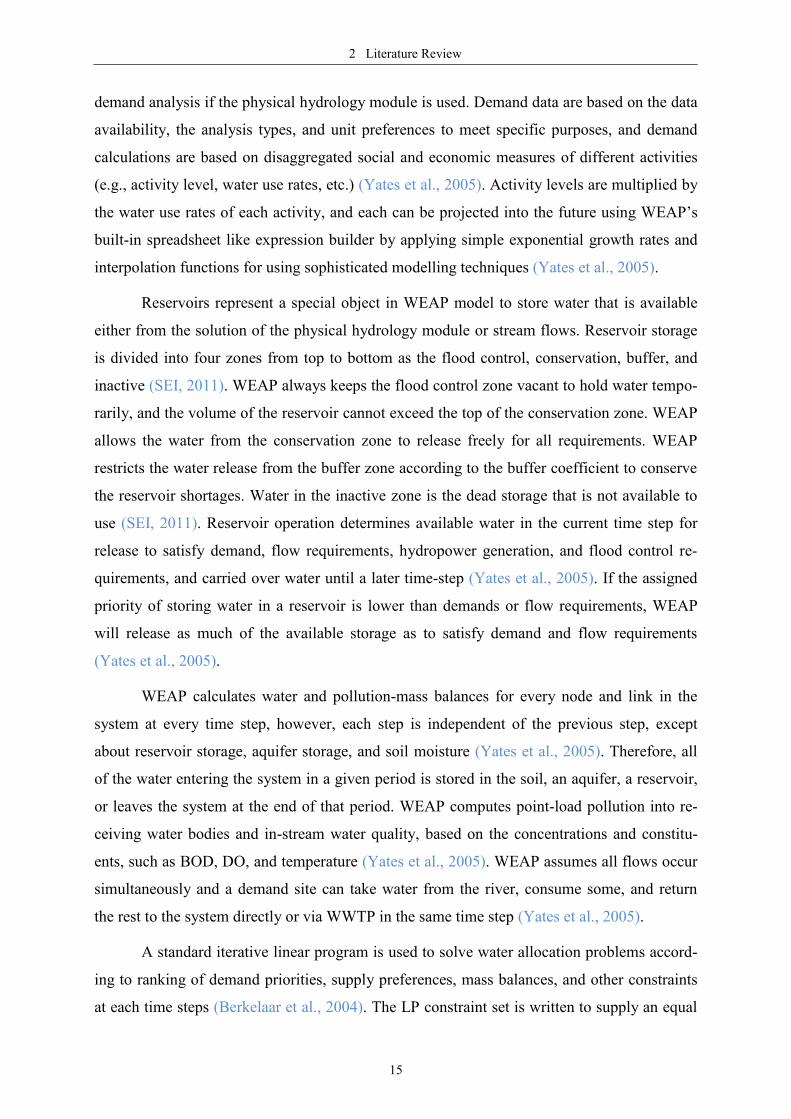
Figure 3.2: Long-term monthly averages for mean daily maximum and minimum temperature (1991-2013) .. 22
Figure 3.3: Long-term monthly average for daily relative humidity of Yangon Region (1991-2013) .............. 22
Figure 3.4: Long-term monthly average for mean daily wind speed of Yangon Region (1991-2013) .............. 23
Figure 3.5: Long-term monthly average for mean sunshine hours per day of Yangon Region (1991-2013) ..... 23
Figure 3.6: Long-term monthly average evaporation of Yangon Region (1991-2013) ..................................... 24
Figure 3.7: Long-term monthly average for monthly rainfall in Yangon Region (1991-2013) ......................... 24
Figure 3.8: Historical population and an estimated population of Yangon City (1800-2040) ........................... 26
Figure 3.9: Urbanization trend of Yangon City with different zones ................................................................. 28
Figure 3.10: Land use map of Yangon City and its surroundings (2012) ............................................................ 29
Figure 3.11: Organization chart of Yangon City Development Committee ......................................................... 31
Figure 3.12: Organization chart of Engineering Department (Water & Sanitation) ............................................ 32
Figure 3.13: Current Water Supply System of Yangon City in 2013 (JICA & YCDC, 2014) ............................ 37
Figure 4.1: Conceptual Modelling Framework of WEAP ................................................................................. 46
Figure 4.2: Simplified schematic for WEAP model of YCWSS ........................................................................ 47
Figure 4.3: Meteorological stations of DMH around Yangon City .................................................................... 54
Figure 4.4: Volume Elevation Curves of Reservoirs in YCWSS ....................................................................... 57
Figure 4.5: Zones of reservoirs in WEAP model (SEI, 2011) ............................................................................ 58
Figure 5.1: The basic concept of scenario analysis in IWRM model (Immerzeel & Droogers, 2008) .............. 64
Figure 5.2: Different options for future water supply in Yangon City ............................................................... 68
Figure 5.3: Forecasted data for future population growth rate ........................................................................... 69
Figure 6.1: Observed volumes and simulated volumes of (a) Gyobyu Reservoir (b) Hlawga Reservoir (c)
Phugyi Reservoir (d) Ngamoeyeik Reservoir (2005-2013) ............................................................. 77
Figure 6.2: (a) Demand coverage (b) Supply delivered amount in Yangon City (2013) ................................... 79
Figure 6.3: Future demand of Yangon City in Reference scenario (a) 2013-2040 (b) monthly average ........... 79
Figure 6.4: Reference Scenario results of (a) Supply delivered and (b) Demand site coverage in Yangon City
(2013-2040) ..................................................................................................................................... 80
Figure 6.5: Unmet demand of Yangon City in Reference Scenario (2013-2040) .............................................. 81
Figure 6.6: Runoff flow from (a) Gyobyu (b) Hlawga (c) Phugyi (d) Ngamoeyeik (e) Lagunpyin catchments to
respective reservoirs of YCWSS (2013-2040) ................................................................................ 82
Figure 6.7: Simulated reservoir storage volumes and zones of (a) Gyobyu (b) Hlawga (c) Phugyi (d)
Ngamoeyeik (e) Lagunpyin reservoirs of YCWSS (2013-2040) ..................................................... 83
Figure 6.8: Groundwater storage changes in different groundwater sources of YCWSS (2013-2040) ............. 83
Figure 6.9: Demand site coverage of Yangon under different external driven scenarios (2013-2040) .............. 84
Figure 6.10: Unmet demand of Yangon City under different external driven scenarios (2013-2040) ................. 85
Figure 6.11: Demand Coverage of Yangon City under management scenarios (2013-2040) .............................. 87

Water supply options for the growing megacity of Yangon - scenarios with the WEAP model
X
Figure 6.12: Unmet demand of Yangon City under management scenarios (2013-2040) ................................... 88
Figure 6.13: Comparison of water coverage in Yangon City under different scenarios (April, 2040) ................ 90
Figure 6.14: Comparison of Unmet demand in Yangon City under different scenarios (April, 2040) ................ 91
Figure 6.15: (a) Demand Site Coverage and (b) Unmet Demand of Yangon City under Reference Scenario and
HPG with HLS Scenario (2013-2040) ............................................................................................. 91
Figure 6.16: Demand site coverage results in Yangon City under possible management scenarios (2013-2040) 92
Figure 6.17: Demand site reliability of Yangon City under different integrated management scenarios ............ 92
Figure 6.18: Demand site coverage of Yangon City under HPG, HLS scenario with four management strategies
(2013-2040) ..................................................................................................................................... 93
Figure 6.19: (a) Demand Site Coverage and (b) Unmet Demand of Yangon City under Reference Scenario and 3
Strategies w/o new project Scenario (2013-2040) ........................................................................... 94

Water supply options for the growing megacity of Yangon - scenarios with the WEAP model
XI
List of tables
Table 1.1: Population trend of Yangon City ........................................................................................................ 4
Table 3.1: Area, Population, Population Growth, and Density in Townships of Yangon City (2013) .............. 27
Table 3.2: Current water sources of Yangon City Water Supply System .......................................................... 35
Table 3.3: Reservoirs of Yangon City Water Supply System ............................................................................ 35
Table 3.4: Aged transmission main pipes in YCWSS ........................................................................................ 36
Table 3.5: Demand coverage of the YCWSS in 2013 ........................................................................................ 38
Table 3.6: Number of connection based on category of water uses in December 2013 ..................................... 39
Table 3.7: Water consumption amount of different water uses in December 2013 ........................................... 39
Table 3.8: Non-revenue water analysis of YCWSS ........................................................................................... 40
Table 3.9: Major problems facing in YCWSS ................................................................................................... 41
Table 3.10: Service level target of YCWSS (JICA & YCDC, 2014) ................................................................... 43
Table 3.11: Proposed future development projects of YCWSS (JICA & YCDC, 2014) ..................................... 44
Table 4.1: Demand sites data of YCWSS-WEAP model ................................................................................... 52
Table 4.2: Location data of meteorological stations around Yangon Region .................................................... 53
Table 4.3: Catchments data of YCWSS-WEAP model ...................................................................................... 55
Table 4.4: Physical data of local reservoirs in YCWSS-WEAP model.............................................................. 56
Table 4.5: Operation data of reservoirs in YCWSS model ................................................................................ 59
Table 4.6: Data of groundwater sources of YCWSS .......................................................................................... 60
Table 4.7: Data of Transmission links in YCWSS ............................................................................................. 62
Table 4.8: Data of Return Flows in YCWSS ..................................................................................................... 62
Table 5.1: Data of Lagunpyin Catchment and Lagunpyin reservoir in YCWSS................................................ 66
Table 5.2: Performance Indicators of water supply service in cities of Southeast Asia countries ..................... 70
Table 5.3: Survey data for river water source (JICA & YCDC, 2014) .............................................................. 75

Water supply options for the growing megacity of Yangon - scenarios with the WEAP model
XII
Lists of Abbreviations
CBD Central Business District
DMH Department of Meteorology and Hydrology (Myanmar)
DSS Decision Supply System
EDWS Engineering Department (Water & Sanitation)
GCM Global Climate Model
gpcd imperial gallons per capita per day
IUR Inner Urban Ring
IWRM Integrated Water Resources Management
JICA Japan International Cooperation Agency
MGD Million Imperial Gallons per Day
MoAI Ministry of Agriculture and Irrigation
NewSZ New Suburbs Zone
NRW Non-Revenue Water
NSZ Northern Suburbs Zone
OldSZ Older Suburbs Zone
ORZ Outer Ring Zone
PIS Performance Indicators
PS Pumping Station
RCP Representative Concentration Pathway
RWH Rainwater Harvesting
SCBD South of Central Business District
SEI Stockholm Environmental Institute
SEZ Special Economic Zone
TS Township
WEAP Water Evaluation And Planning
WTP Water Treatment Plant
WWTP Waste Water Treatment Plant
YCDC Yangon City Development Committee
YCWSS Yangon City Water Supply System
Water supply options for the growing megacity of Yangon - scenarios with the WEAP model
XIII
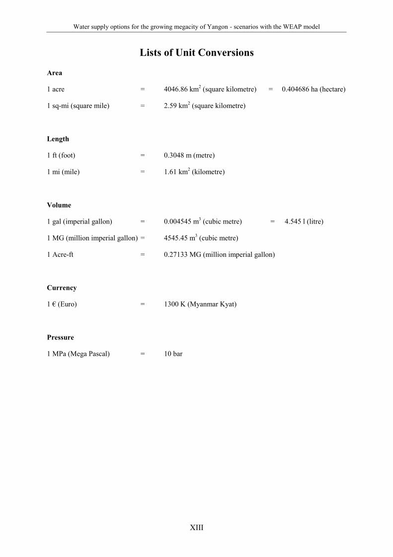
Lists of Unit Conversions
Area
1 acre = 4046.86 km2 (square kilometre) = 0.404686 ha (hectare)
1 sq-mi (square mile) = 2.59 km2 (square kilometre)
Length
1 ft (foot) = 0.3048 m (metre)
1 mi (mile) = 1.61 km2 (kilometre)
Volume
1 gal (imperial gallon) = 0.004545 m3 (cubic metre) = 4.545 l (litre)
1 MG (million imperial gallon) = 4545.45 m3 (cubic metre)
1 Acre-ft = 0.27133 MG (million imperial gallon)
Currency
1 € (Euro) = 1300 K (Myanmar Kyat)
Pressure
1 MPa (Mega Pascal) = 10 bar

1 Introduction
1
1 Introduction
Water, a precious natural resource, is vital for physiological processes of all organ-
isms. Moreover, water also has a social and economic value for human beings, and on the
other hand, population growth and economic development put constant pressure on the eco-
systems of water resources (Alcamo et al., 2007). There is a strong positive correlation be-
tween water demand and urbanization or population growth (Malmqvist & Rundle, 2002).
Urban water system should provide safe water for different uses without harming the envi-
ronment, and increasing demand for sustainable development will deeply affect on all urban
infrastructures (Hellström et al., 2000). Therefore, sustainable management of water supply
for various water uses in urbanized cities is extremely important to achieve the sustainable
development of these cities. Comprehending the urban growth and clearly explaining options
are two main requirements for effective decision-making about sustainable development of
urban infrastructure (Grigg, 1997).
Cities emerge and grow accompanied with population growth because of human re-
sources and labour force availability and their attraction to economic activities (Haughton &
Hunter, 2004). For example, Yangon City, the biggest city of Myanmar and also commercial
and financial capital of Myanmar, experienced higher population growth rate about 2.8% be-
tween a decade from 1993 to 2003, whereas the national population growth rate was less than
2% (Aung, 2013). Yangon City is undergoing accelerated urbanization and rapid development
as the nation moves towards democracy. Yangon City, its population is 5.14 million at present
and expected to reach above10 million in 2040 together with both urbanization and industrial-
ization, is forecasted to become a megacity in the future (Yangon Region Government,
YCDC & JICA, 2013).
As the other urbanized cities of the world, population of Yangon City is increasing
alarmingly together with the city area, and this is exerting more pressure on it’s existing old
infrastructures including the water supply system. Currently, insufficient data and lack of the
plan for the future are restricting the management of the water supply system of Yangon City
and the decision making for future options for various urban issues.

1 Introduction
2
1.1 Background
Myanmar, officially “the Republic of the Union of Myanmar,” is one of the Southeast
Asia countries and surrounded by the Andaman Sea, the Bay of Bengal, Bangladesh, India,
China, Laos, and Thailand. Its total area is 676,552 km2, the world’s 40
th largest country and
the second largest country in Southeast Asia, and its population has increased from 28.9 mil-
lion in 1973 to over 60 million in 2009 (Morley, 2013). Myanmar has abundant natural re-
sources and sizeable workforce for domestic manufacturing and industries (Morley, 2013). In
the report of the Immigration and Manpower Department (Ministry of Immigration and Popu-
lation), the total population of the Union of Myanmar in 2012 is 63.5 million. Political reform
has recently occurred in Myanmar, and a new constitution was approved in 2008 and then the
first general election was held in November 2010. As a consequence, Present-day Myanmar is
a place encountering rapid transformation in every sector and largely investing in infrastruc-
ture for economic development. According to International Monetary Fund (IMF, 2014), My-
anmar’s Gross Domestic Product (GDP) using current prices grew from $7.45 billion in 1998
to $56.4 billion in 2013.
Figure 1.1: A map of Myanmar and Yangon Region

1 Introduction
3
In the new constitution of the Republic of the Union of Myanmar (2008), Myanmar is
divided into 21 administrative subdivisions; 1 Union Territory, 7 States, 7 Regions, 5 Self-
administered Zones, 1 Self-administered Division. Among 7 regions, the Yangon region has
the smallest land area, only 1.5% of the total country’s area, however, it has the highest popu-
lation in all subdivisions, 12% of the national population. The above Figure 1.1 shows the
map of Myanmar and Yangon Region.
Yangon City, the former national capital of Myanmar, is the capital city of Yangon
Region and the largest city of Myanmar. Yangon is not only the centre for transportation and
commercial activities in Myanmar but also the centre for all opportunities in education and
health services (Khaing, 2006). Yangon City has an area of 794.4 km2 with 33 townships, and
it is one of the largest spatial extent cities in South East Asia (Morley, 2013). Even though the
national capital of Myanmar was moved to Naypyidaw, a new administrative city situated
about 320 km north of Yangon City, in 2006, Yangon is still important for nation’s economy,
culture and social issues. Yangon City is the largest urban agglomeration area in Myanmar,
and it contributes 22% of the national GDP (Aung, 2013). Nowadays, Yangon is undergoing
major alterations in its economic, social and infrastructures accompanied with country’s
changes.
The following Table 1.1 shows the historical population trend of Yangon City against
city’s spatial extent, population density and population growth rate (Census of India, 1891;
Census of India,1901; Census of India,1911; YCDC, 2014b). The population of Yangon City
speedily elevated from about 3.1 million in 1993 to over 5.14 million in 2013 with a growth
rate 2.56% (Yangon Region Government, YCDC & JICA, 2013). The future population
growth rate of Yangon City is likely to be the same rate or may even increase due to political
changes and national development plans, such as, Plan of Economic zone at Thilawa, Plan of
the new international airport near Bago, and also due to the growth and attraction of the city
itself (Aung, 2013). With the same population growth rate 2.56%, the population of the city
will have more than 10 million in 2040 (Yangon Region Government, YCDC & JICA, 2013).
Yangon City Water Supply System has a long history. Although Yangon City water
supply services initiated since 1842, service coverage is still only 30 % of the whole city and
non-revenue water is 66 % of total daily supply water amount (JICA & YCDC, 2013). Ap-
proximately 90 % of the total supply water to Yangon City comes from surface water via
drinking water reservoirs and the rest comes from tube wells, however, water treatment sys-
tem is insufficient and needs to improve qualitatively and also quantitatively. Water charge is

1 Introduction
4
quite low comparing with other countries, about 0.068 € (88 MMK) per m3 for domestic use
and 0.085 € (110 MMK) per m3 for commercial use, so that it cannot be secure to get finan-
cial sources for operation and maintenance of water supply system. On one side, there are
many requirements for improvement in the operation and maintenance of existing water sup-
ply system, and on the other side, there will be necessary to analyse and prepare for the future
challenging boosted water demand in association with alarming increased population.
Table 1.1: Population trend of Yangon City
(Source: Population data are obtained from Department of Population, Ministry of Immigration and
Population. Data from 1881 to 1931 is derived from censuses of India, data from 1953 to
1983 come from national censuses, and data from 1993 to 2013 is estimated. Area data are
acquired from Urban Planning Division, YCDC, and History of Yangon City retrieved from
the official website of YCDC.)
Year Population
(million)
Population
Growth Rate
(%)
Area
(km2)
Population
Density
(person/km2)
Remark
1800 0.0300 - ~ 2.0 - -
1851 0.0400 0.1 No data - -
1861 0.0600 4.1 No data - -
1871 0.0987 5.2 No data - -
1881 0.1342 3.0 28.49 4710 Expansion in 1876
1891 0.1803 3.0 49.21 3664 Expansion in 1880s
1901 0.2349 3.2 49.21 4773 -
1911 0.2933 1.7 72.52 4044 Expansion in 1900s
1921 0.3419 1.5 79.77 4286 Expansion in 1910s
1931 0.4004 1.6 79.77 5019 -
1953 0.7370 2.8 123.3 5977 Expansion in 1930s & 1940s
1963 0.9400 2.5 164.2 5725 Expansion in late 1950s
1973 2.0152 7.9 221.4 9102 Expansion 1965 and 1973
1983 2.5130 2.2 346.0 7263 Expansion in 1983
1993 3.0978 2.1 603.5 5133 Expansion in 1991
2003 4.1000 2.8 794.4 5161 Expansion in 2003
2013 5.1400 2.3 794.4 6470 -

1 Introduction
5
In order to solve the problems of existing and future water supply system of Yangon
City, many processes are necessary to establish for the development of the water supply sys-
tem of growing megacity Yangon. For example, formulation of the water management model
and plan for the future scenario analysis, investigation of potential water resources, alternation
of systems and technologies, maintenance of the old system, implementation of new water
facilities etc. At present, Yangon City Development Committee (YCDC), a local administra-
tive organization for Yangon City, has been formulating the project for the strategic urban
development plan of Greater Yangon (Yangon City and 6 peripheral townships (Kyauktan,
Thanlyin, Hlegu, Hmawbi, Htantabin, Twantay) with the coordination of Japan International
Cooperation Agency (JICA) and other local and global organizations. A study on the im-
provement of water supply in Yangon City is also one of the topics included in this project.
However, due to various reasons and restrictions, for instance, lack of systematic data and up-
to-date water resources management knowledge, Yangon City is encountering problems to
establish the improvement of water supply system, and it is limited in its ability to respond to
these problems.
1.2 Study problem
Yangon City Water Supply System (YCWSS) is experiencing water supply facilities
operation and management problems, and on the other hand, rapid urbanization and industri-
alization together with increasing population, are challenging the water supply system of
Yangon City. Therefore, organizations, which are responsible for the water supply of Yangon
City, require putting efforts to solve these problems as well as to find the new water resources
for increasing water demand.
So, it is required to formulate the future development plans and management strategies
for water supply system of Yangon City by using different possible future scenarios. It is also
needed to compare and contrast these different scenarios, and then recommend the best effec-
tive and sustainable plan in order to contribute to economic development and improvement of
the living environment of Yangon City. It is also necessary to forecast water demand and sup-
ply of the City in the future for operation and management of the city water supply system
and new projects and plans. Using a water supply-demand modelling tool is the best approach
to solve these problems.
1 Introduction
6
1.3 Study objective
The main objective of this study is to develop Water Evaluation And Planning
(WEAP) model for the water supply system of Yangon City, which will be used to analyse
the different scenarios for the future water supply against with the growing water demand.
In order to reach this study objective, the tasks need to be done are:
To describe the overview of the current situation of Yangon City water supply
To analyse the status quo and future scenarios of water supply system
To evaluate and make recommendations for these different future scenarios
1.4 Study methodology
In this thesis, firstly, publications from WEAP website and other research literature are
collected and reviewed, focusing on the water supply demand models of large cities and about
WEAP modelling especially for developing countries in monsoon regions.
Secondly, reports and documents of Engineering Department (Water & Sanitation),
YCDC are studied and reviewed to extract the data, which are reliable as an official data and
are applicable as an input data for the purpose of the study. Moreover, Water Supply Master
Plan 2002 and 2014, formulated by YCDC and JICA, are also reviewed to get the data relat-
ing to the current water supply system analysed data, customer survey data, and feasibility
study data of new water resources for future projects.
Thirdly, field research was done to collect the data of water supply and demand data in
actual condition, for instance, visiting the water supply reservoirs of Yangon City to collect
the water supply data and visiting the offices of different divisions of EDWS to collect the
actual water supply-demand and water uses data.
Finally, WEAP model is applied to quantify and observe the positive and negative im-
pacts of future scenarios, also to give recommendations for the future implemented projects.
In the WEAP model, demand-side and supply-side management scenarios are explored, and
then analysed their behaviours by simulation. WEAP model is used as an analysis instrument
to understand the impacts of the water supply system of Yangon City at present and future.
By discussing the results of the model, impacts of scenarios that can be taken in more consid-
erations and options, which can be used as recommendations, are evaluated and highlighted.
To sum up, methods used in this study are literature review, official report and docu-
ment review, field research and WEAP modelling.
1 Introduction
7
1.5 Structure of the Thesis
The thesis is organized and presented with seven parts. They are as follows:
(1) Introduction
In this part, the background of the thesis, the study problem, the study objective, and
the study methodology will be introduced.
(2) Literature Review
In this part, firstly, the idea of the water management models will be described by re-
viewing research literature. Then, the literature review of WEAP model will be presented.
Finally, the application of WEAP model in different countries, especially in urban regions,
will be highlighted by using WEAP model studies.
(3) Yangon City Water Supply System (YCWSS)
In this part, an overview of the study area, Yangon City, will be presented by express-
ing the current situations. After that, the study organization, Yangon City Development
Committee and its department, Engineering Department (Water & Sanitation), will be de-
scribed. At last, the past and present water supply system of Yangon City will be expressed by
analysing the reports and documents from water-authorised organizations.
(4) Development of WEAP model for YCWSS
In this part, a WEAP model for water supply system of Yangon city will be developed
and simulated not only to evaluate for Today’s water supply system and water demand, but
also to estimate Future demand.
(5) Creation of scenarios in WEAP
In this part, different scenarios for the future of Yangon City, such as, population
growth, economic development, climate change, demand side management, and supply side
management, will be created.
(6) Simulation and Evaluation of scenarios
In this part, the evaluation of the simulated results of the scenarios will be done by
comparing and contrasting the future development impacts and examining the reliability of
the water supply system.
(7) Discussions and Recommendations
In this part, future options for the water supply system of Yangon City will be dis-
cussed based on the results of WEAP model simulations. After that, recommendations for
long-term planning of the water supply system of Yangon City will be presented.

2 Literature Review
8
2 Literature Review
Many regions are facing alarmingly challenges about water management as well as
limited water resources allocation, environmental quality and sustainable water use policies
are increasing concerned issues. Over the last decade, an integrated water development ap-
proach has emerged and replaced for the conventional supply-oriented simulation models, and
which aimed to develop the context of demand-side, water quality and ecosystem preservation
issues in water supply projects. To explore options for the future, the appropriate simulation
models are required to see how the impact of future trends will occur and how we can adapt to
these in the most sustainable way.
This part will describe about the background knowledge of the water management
models and the modelling of water availability and demand for large cities by reviewing the
literature. At first, water supply-demand management models will be discussed. After that,
WEAP model will be introduced according to the publications from WEAP website. At last,
the review of the application of the WEAP model in different countries and different water
basins, focusing on urban water management issues, will be presented.
2.1 Water Resources Management Models
Water resources planning and management was generally an exercise-based on engi-
neering considerations in the past. Nowadays, it increasingly occurs as a part of complex,
multi-disciplinary analysis that brings together a wide range of individuals and organizations
with different interests, technical skills, and options (Yates et al., 2005; Hamlat, Errih & Gui-
doum, 2013). Successful planning and management of water resources requires application of
effective integrated water resources management (IWRM) models that can solve the encoun-
tering complex problems in these multi-disciplinary investigations (Loucks, 1995; Laín,
2008).
Water resource planning and management processes aided IWRM models have be-
come more common, however generic tools that can be applied to different basin settings are
frequently difficult to use because of the complex operating rules that govern individual water
resource systems (Watkins and McKinney, 1995). IWRM models, which can incorporate and
operate hydrology and management processes at the same time, are needed to help planners
2 Literature Review
9
under different reality cases and management options (Yates et al., 2005). These IWRM mod-
els must be effective, useful, easy-to-use, and adaptive to planners’ priorities.
Effective IWRM models must deal with the biophysical system, which create runoff
generation and its movement, and the socioeconomic management system, which create water
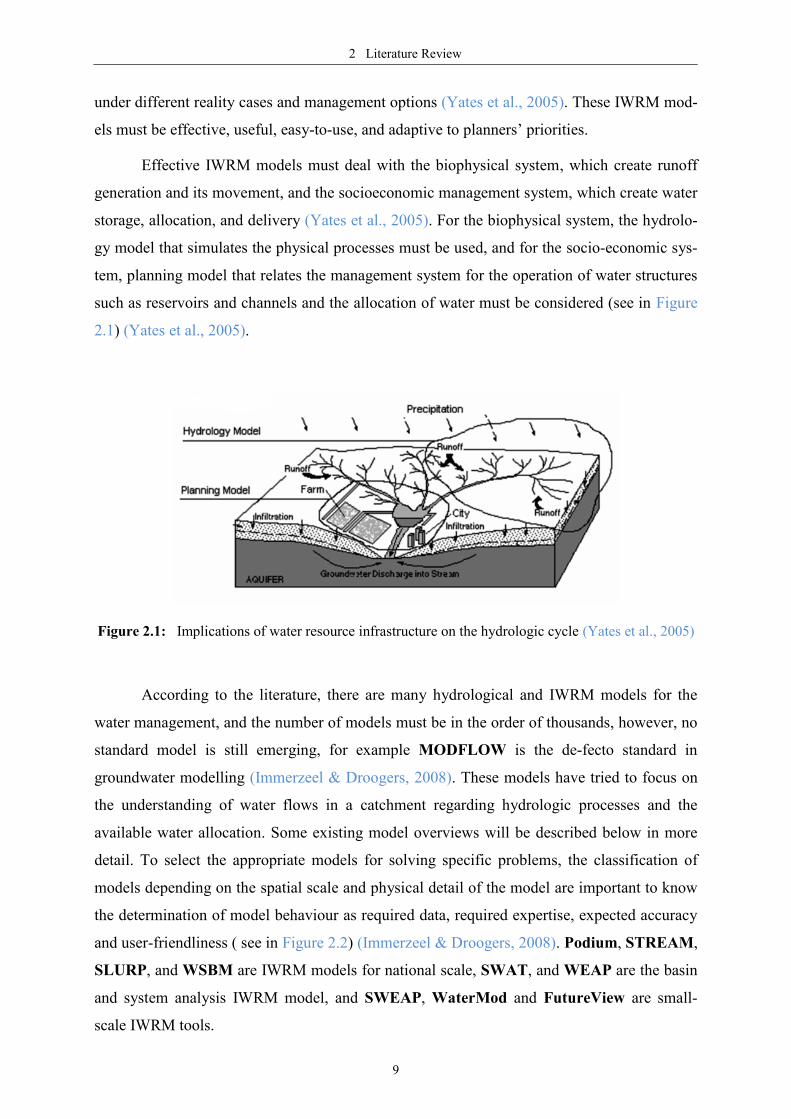
storage, allocation, and delivery (Yates et al., 2005). For the biophysical system, the hydrolo-
gy model that simulates the physical processes must be used, and for the socio-economic sys-
tem, planning model that relates the management system for the operation of water structures
such as reservoirs and channels and the allocation of water must be considered (see in Figure
2.1) (Yates et al., 2005).
Figure 2.1: Implications of water resource infrastructure on the hydrologic cycle (Yates et al., 2005)
According to the literature, there are many hydrological and IWRM models for the
water management, and the number of models must be in the order of thousands, however, no
standard model is still emerging, for example MODFLOW is the de-fecto standard in
groundwater modelling (Immerzeel & Droogers, 2008). These models have tried to focus on
the understanding of water flows in a catchment regarding hydrologic processes and the
available water allocation. Some existing model overviews will be described below in more
detail. To select the appropriate models for solving specific problems, the classification of
models depending on the spatial scale and physical detail of the model are important to know
the determination of model behaviour as required data, required expertise, expected accuracy
and user-friendliness ( see in Figure 2.2) (Immerzeel & Droogers, 2008). Podium, STREAM,
SLURP, and WSBM are IWRM models for national scale, SWAT, and WEAP are the basin
and system analysis IWRM model, and SWEAP, WaterMod and FutureView are small-
scale IWRM tools.

2 Literature Review
10
Figure 2.2: Spatial and physical detail of hydrological models (Immerzeel & Droogers, 2008)
SWAT (Soil and Water Assessment Tool) includes complex physical hydrology mod-
ules as rainfall-runoff, irrigated agriculture, and point and non-point catchment dynamics, but
it is a relatively simple reservoir operations module (Srinivasan, 1998; Neitsch et al., 2002;
Fontaine et al., 2002). This model is originating from United States Environmental Protection
Agency’s research program, and it might have the potential to be a de-facto standard in basin
scale modelling (Immerzeel & Droogers, 2008).
RiverWare™ DSS is a hydrology and hydraulics operations model, and can be used
to develop multi-objective simulations and optimizations of river and reservoir systems like
river reaches, diversions, storage reservoirs, hydropower reservoirs, and water uses, but it
needs to upstream flow acquired from a physical hydrologic model (Zagona et al., 2001).
US Geological Survey’s Modular Modelling System gives a framework for integra-
tion with RiverWare by using such the Precipitation Runoff Modelling System to supply
boundary flows (Leavesley et al., 1983). US Army Corp of Engineers’ HEC-ResSim is a res-
ervoir simulation model, and can show the operating rules and requirements, but it needs pre-
scribed flows from other models (Klipsch, 2003).
MODSIM DSS is a generalized river basin model, and incorporate the complex phys-
ical, hydrological, and administrative basin management, but it requires boundary flows
(Labadie et al., 1989). MULINO DSS (Multi-sectoral, Integrated and Operational Decision
Support System) is a decision support system for sustainable use of water resources at the
catchment scale focusing on multi-criteria decision aid, and it can link an external physical
hydrology model by appropriate input-output procedures (Giupponi et al., 2004).
WaterWare is a sophisticated decision support system and includes dynamic simula-
tion about physical hydrology (water quality, allocation, rainfall-runoff, groundwater) and

2 Literature Review
11
water management (demand-supply, cost-benefit analysis, and multi-criteria analysis), but it
requires a complicated user/hardware support (Jamieson & Fedra, 1996; Fedra & Jamieson,
1996).
RIBASIM (River Basin Model) is a comprehensive and flexible model for analysing
the behaviour of river basins under various hydrological conditions to evaluate the operation
and management measures in terms of water quantity and quality (Krogt, 2003; Loucks, 2006;
Mugatsia, 2010). It provides a source analysis, giving insight into the water's origin at any
location of the basin. It utilizes various hydrologic routing methods to execute the flow on a
daily basis, and provides water distribution patterns, source analysis, and water quality and
sedimentation analysis in reservoirs and river (Krogt, 2003; Loucks, 2006; Mugatsia, 2010),
and is applied for river basin planning and management in different projects in countries
around the world. However, this model requires good data based infrastructures to build the
input data.
MIKE BASIN is a hydrologic modelling with ArcGIS to provide basin-scale solu-
tions of water allocation, conjunctive use, reservoir operation and water quality issues by
simulation and visualization in space and time (Loucks, 2006; Assata et al., 2008). It is a qua-
si-steady-state mass balance model for river flows routing, and assuming purely advective
transport for the water quality analysis and using the linear reservoir equation for the ground-
water analysis (Loucks, 2006; Assata et al., 2008). It requires to link with a separate hydro-
logical model like NAM, or MIKE SHE of DHI to perform an integrated catchment manage-
ment system, and the model data requirement has constraints, such as complete discharge
time series, accurate spatial water abstraction data etc. (Loucks, 2006; Assata et al., 2008).
WBalMo (Water Balance Model) is an interactive simulation tool for river-basin
management, and it simulates the natural processes of runoff and precipitation stochastically
by balancing the respective time series with monthly water use demands and reservoir storage
changes (Loucks, 2006; Mugatsia, 2010). It can identify management guidelines for river ba-
sins, design reservoirs and their operations, and perform scenario analysis and environmental-
impact analysis for development projects, but it requires detailed data for design purposes
(Loucks, 2006; Mugatsia, 2010).
WEAP (Water Evaluation And Planning) model tries to fill the gap between water re-
sources management and physical hydrology, and integrates the management of demands and
water facilities with physical hydrologic processes in a simple and perfect way (Yates et al.,
2005). WEAP is effective, useful, easy-to-use, affordable, and readily available. It can also

2 Literature Review
12
analyse multiple scenarios, including climate change scenarios and other changes, such as
technical changes, social-economic changes, and policy changes. For example, land use
changes, municipal and industrial demands changes, operating rules changes, etc. The main
aim of WEAP is to solve the water planning and resource allocation problems and issues, but
can also analyse the water quality, cost-benefit, and hydropower based on hydrological pro-
cesses (Yates et al., 2005; SEI, 2011).
The best approach for IWRM models is to develop a straightforward and flexible tool
to assist rather than to substitute the skilled water professionals, the users of the model (SEI,
2011). WEAP is a new generation of water planning and management software, and the pow-
erful capability of today’s personal computers can easily use it everywhere to access to the
appropriate tools.
2.2 WEAP model
WEAP modelling software developed by the Stockholm Environmental Institute (SEI)
is an object-oriented computer-modelling package and IWRM tool, designed for simulation of
water supply system and demand analysis, and WEAP is a laboratory for analysing alternative
water management and development strategies (SEI, 2011). WEAP approaches to simulate
water systems by its policy orientation, and balances the demand side (water uses, equipment
efficiencies, water reuse, prices, hydropower energy demand, and water allocation) and the
supply side (streamflow, groundwater, reservoirs, and water transfers) (SEI, 2011). The basic
principle of WEAP is a water balance accounting operation with monthly time step, and it can
be applied in a single catchment to a complex trans-boundary river basin (SEI, 2011). WEAP
can analyse a wide range of issues, such as water demand, water conservation, water quality,
water rights, allocation priorities, groundwater, streamflow, reservoir operations, hydropower
generation, energy demands, ecosystem requirements, and project cost-benefit (SEI, 2011).
In WEAP, the time horizon and spatial boundary of the study, components of the sys-
tem, and configuration of the problem are needed to set up. WEAP represents the system with
supply sources, demand sites, transmission links, wastewater treatment plants, ecosystem re-
quirements, and pollution generation, and analyses with the customized data structure and
level of detail to meet the requirements and restrictions (SEI, 2011). WEAP’s objects and
model-framework are graphically oriented to allow the spatial referencing of attributes, e.g.
river and groundwater, demand sites, WWTPs, catchments and political boundaries, and river
reach lengths etc. (SEI, 2011). WEAP model simulates as a set of scenarios and simulation

2 Literature Review
13
time steps can be daily, weekly, monthly, and seasonally with a time horizon from a single
year to more than 100 years (SEI, 2011).
The Current Accounts in WEAP represents the overview of actual water demand, wa-
ter supply sources, supplies for the system, pollution loads, at the current year or a baseline
year (SEI, 2011). Scenarios are alternative sets of future options based on different policies,
different management strategies, different economic, demographic, hydrological and techno-
logical trends, over the time horizon of the study (SEI, 2011). Scenarios are evaluated based
on demand coverage, costs and benefits, compatibility with targets, and sensitivity to key var-
iables uncertainty (Yates et al., 2005).
A number of methodological considerations, such as integrated and comprehensive
planning framework, scenario analyses of the effects of different development options, de-
mand-management capability, environmental assessment capability, ease-of-use, and urban
water planning and management, designs WEAP model (SEI, 2011).
WEAP integrates demand and supply, water quantity and quality, and economic de-
velopment objectives and environmental constraints, and evaluates specific water problems in
a comprehensive framework (SEI, 2011). In WEAP, Current Accounts and Reference scenar-
io or business-as-usual scenario need to create first, and then other alternative policy scenari-
os can be developed for comparison of their effects on the system against the business-as-
usual scenario (SEI, 2011). The business-as-usual scenario represents the current situation of
economic and demographic development, water supply and demand, policy, and other aspects
without any alternatives. WEAP can also represent the effects of demand management on
water systems, for example, the effects of water pricing policy or priorities for allocation wa-
ter demand and sources, improved technologies (SEI, 2011). WEAP can provide the require-
ments for aquatic ecosystems such as concentration of river water quality, pollution pressure
of different water uses on the overall system by tracking from subject to object (SEI, 2011).
WEAP has a user-friendly interface with graphical drag-and-drop GIS-based inputs and out-
puts as maps, charts, and tables. The WEAP’s intuitive graphical interface is simple but pow-
erful to construct, view, and modify the system and its data, and WEAP handles loading data,
calculating and reviewing results with an interactive screen structure, which catches errors,
provides on-screen guidance and prompts the user (SEI, 2011). In WEAP, the data structures
are expandable and adaptable to evolving needs of water analysts as better information be-
come available, and planning changes, and users’ own set of variables and equations can de-
velop for further analysis of specific constraints and conditions (SEI, 2011).

2 Literature Review
14
WEAP is adaptable and flexible to all available data, i.e. daily, weekly, monthly, or
annual time-steps, to describe the system's water supplies and demands, i.e. it can be applied
in a range of spatial and temporal scales (SEI, 2011). At past, WEAP has been used to assess
the reliability of water supply and the sustainability of surface water and groundwater sup-
plies in future scenarios of the proposed management and project. At present, WEAP model
can be used in the urban water management integrating storm water, wastewater, and water
supply, by using updated features, such as infiltration and inflow, infiltration basins & reten-
tion ponds, display of user-defined performance measures as results, tiered water pricing,
combined sewer overflows (SEI, 2011). WEAP can link to other models and software, such as
QUAL2K (surface-water quality model), MODFLOW (groundwater flow model), MOD-
PATH (a particle-tracking model for MODFLOW), PEST (parameter estimation tool),
GAMS (general algebraic modelling system), Excel, and Google Earth (SEI, 2011; WEAP,
2014).
WEAP is based on the most basic idea, water supply depends on the amount of rain-
falls on a catchment or a series of catchments, which is progressively decreased through natu-
ral hydrological processes, human demands, or increased through catchment enlargement
(Yates et al., 2005). WEAP includes a water balance model for hydrologic processes within a
catchment system and that can address the propagating and non-linear effects of different wa-
ter uses, and also includes a point-source pollutant loading descriptive model that can simu-
late the impacts of wastewater on receiving waters (Yates et al., 2005).
The basic idea in the WEAP water management analysis is the development of differ-
ent water demands such as municipal, industrial, irrigation, and ecosystem requirements, with
user-defined priority (given as an integer from 1 to 99, highest to lowest priority), and each
demand links to its available supply sources with user-defined preference (Yates et al., 2005).
The supply-demand network is constructed and optimized routine that allocates available
supplies to all demands. Demand analysis in WEAP is based on the evapotranspiration and
the disaggregated end-use that determines water requirements at each demand node. Explor-
ing by scenarios use demographic and water-use information, and WEAP computes all supply
and demand sites by applying Linear Program (LP) allocation algorithm, which determines
the final delivery to each demand node, based on the user-defined priorities (Yates et al.,
2005).
Demand sectors can be disaggregated into different sub-sectors, end-uses, and water-
using devices, but, agriculture and urban water demands are not included in the disaggregated
2 Literature Review
15
demand analysis if the physical hydrology module is used. Demand data are based on the data
availability, the analysis types, and unit preferences to meet specific purposes, and demand
calculations are based on disaggregated social and economic measures of different activities
(e.g., activity level, water use rates, etc.) (Yates et al., 2005). Activity levels are multiplied by
the water use rates of each activity, and each can be projected into the future using WEAP’s
built-in spreadsheet like expression builder by applying simple exponential growth rates and
interpolation functions for using sophisticated modelling techniques (Yates et al., 2005).
Reservoirs represent a special object in WEAP model to store water that is available
either from the solution of the physical hydrology module or stream flows. Reservoir storage
is divided into four zones from top to bottom as the flood control, conservation, buffer, and
inactive (SEI, 2011). WEAP always keeps the flood control zone vacant to hold water tempo-
rarily, and the volume of the reservoir cannot exceed the top of the conservation zone. WEAP
allows the water from the conservation zone to release freely for all requirements. WEAP
restricts the water release from the buffer zone according to the buffer coefficient to conserve
the reservoir shortages. Water in the inactive zone is the dead storage that is not available to
use (SEI, 2011). Reservoir operation determines available water in the current time step for
release to satisfy demand, flow requirements, hydropower generation, and flood control re-
quirements, and carried over water until a later time-step (Yates et al., 2005). If the assigned
priority of storing water in a reservoir is lower than demands or flow requirements, WEAP
will release as much of the available storage as to satisfy demand and flow requirements
(Yates et al., 2005).
WEAP calculates water and pollution-mass balances for every node and link in the
system at every time step, however, each step is independent of the previous step, except
about reservoir storage, aquifer storage, and soil moisture (Yates et al., 2005). Therefore, all
of the water entering the system in a given period is stored in the soil, an aquifer, a reservoir,
or leaves the system at the end of that period. WEAP computes point-load pollution into re-
ceiving water bodies and in-stream water quality, based on the concentrations and constitu-
ents, such as BOD, DO, and temperature (Yates et al., 2005). WEAP assumes all flows occur
simultaneously and a demand site can take water from the river, consume some, and return
the rest to the system directly or via WWTP in the same time step (Yates et al., 2005).
A standard iterative linear program is used to solve water allocation problems accord-
ing to ranking of demand priorities, supply preferences, mass balances, and other constraints
at each time steps (Berkelaar et al., 2004). The LP constraint set is written to supply an equal

2 Literature Review
16
percentage of water to all same-priority demand sites and to choose the supply for a demand
site by supply-preferences rank, because irrigations and municipalities will mostly depend on
multiple water sources to meet their demands (Yates et al., 2005). The LP algorithm iterates
all supply preference to optimize the demand coverage and operates depends on the user-
defined constrains, such as maximum flow volume of transmission links, percent of demand,
physical or contractual limits, besides supply preferences (Yates et al., 2005).
To sum up, WEAP is one of the useful IWRM tools, and capabilities to build complex,
distributed physical hydrology and demand models of municipal, industrial, agricultural, and
environmental demands at different spatial and temporal scales (Yates et al., 2005). WEAP
incorporates a demand priority and a supply preference approach to describe water resource
operating rules. Nowadays, WEAP has been used throughout the world to analyse the variety
of water management issues in small scales to large ones.
2.3 Applications of WEAP model
WEAP model was created in 1988 as a flexible IWRM tool for the current water sup-
ply-demand system evaluation and future scenario exploration (WEAP, 2014). It has a long
history of development and use in the water-planning field. The first major application of
WEAP was in 1989 to study on the water development strategies and water supply-demand
analysis for the Aral Sea region in 1989 with the sponsorship of SEI (Raskin et al., 1992). The
version of WEAP at that time had several limitations, such as an allocation scheme, demand
sites priorities, water allocations (Raskin et al., 1992). Because of these deficiencies, WEAP
introduced major advances, including a modern Graphic User Interface and a robust solution
algorithm to solve the water allocation problem. Moreover, WEAP integrated hydrologic sub-
modules such as a conceptual rainfall-runoff model, an alluvial groundwater model, and a
water quality model (Yates et al., 2005). WEAP software has been supported to water plan-
ners from global organization and institutions, especially, freely transferred to governmental
and academic users from developing countries, and WEAP has been applied in many coun-
tries and river basins over two decades (WEAP, 2014).
Johnson, W. K. (1994) applied WEAP for accounting of Water Supply and Demand in
the upper Chattahoochee River Basin of Georgia, to illustrate the capability of WEAP, to pro-
vide a document for WEAP users how the program is applied in a multiple-use river and res-
ervoir. Purkey, Thomas, Fullerton, Moench & Axelrad (1998) used WEAP in the groundwater
banking feasibility study in California by analysing hydrology, legal & institution, operation

2 Literature Review
17
and economics. Strzepek et al. (1999) introduced new methods of linking IWRM models
(WATBAL for water supply, CERES, SOYGRO, CROPWAT for crop and irrigation model-
ling, and WEAP for planning and water demand forecasting) with climate change scenarios
for the study of future water availability in the U.S. Cornbelt’s agriculture.
Water-demand management scenarios (saving water by individual users with three op-
tions 10%, 20%, and 30%) for diverse climate situations ( dry years to normal years) at the
Steelpoort Sub-basin of the Olifants River in South Africa was tested by using the WEAP
model (Lévite, Sally, & Cour, 2003). Even though there are some limitations of the WEAP
model like as a water year method, the user-friendly model and its interfaces make easy for
discussions and dialogue on water management among decision makers and local stakehold-
ers, and for the promotion of public awareness and understanding of key issues and concerns
(Lévite, Sally, & Cour, 2003).
The application of WEAP models to major agricultural regions in Argentina, Brazil,
China, Hungary, Romania, and the US, was analysed by simulating future scenarios about
climate change, agricultural yield, population, technology, and economic growth (Rosenzweig
et al., 2004). Climate change projection using global climate models (GCM) simulations indi-
cates eventually larger changes in the 2050s and beyond, but the water for the agricultures is
sufficient in most of the water-rich areas (Rosenzweig et al., 2004). Northeastern China shows
the most stressed in water availability for agriculture and ecosystem services both in the cur-
rent state and in the climate change projections (Rosenzweig et al., 2004).
The study about water evaluation and the planning system in Kitui-Kenya clearly
demonstrated that WEAP is a powerful framework in the evaluating of current and future op-
tions of water resources, and evaluation can be performed within a few minutes by adding
more accurate data to increase the accuracy of the analysis and validation of results (Van
Loon & Droogers, 2006). To help decision makers and stakeholders, Integrated Decision
Support System (DSS) for pollution control in the upper Litani Basin of Lebanon was devel-
oped by using WEAP, and this DSS was effectively used in projection of three future scenari-
os for the water quality conditions in the basin (Assaf & Saadeh, 2006).
As population growth, urbanization, and current policies and water management prac-
tices give stresses on water resources and urban infrastructure, urban water management tools
are becoming essential for urban water planners to see the overview of their water system
(O’Connor, Rodrigo, & Cannan, 2010). Urban water systems can be improved by reducing
water demands, increasing water recycling and reuse, creating alternative water supply

2 Literature Review
18
sources from storm water/rain water, providing water quality to end-use needs, and imple-
menting multi-purpose, multi-benefit infrastructure to achieve environmental goals
(O’Connor, Rodrigo, & Cannan, 2010).
WEAP was also applied as an urban water management tool in the study of water re-
sources and city sustainable development of Heng Shui City in China (Ojekunle, 2006). This
study pointed out that the availability and reliability of data are very important and must be
analysed carefully with good judgment, and the adoption of water demand management gives
opportunities during normal hydrological years but not in dry years. This study explored and
evaluated the future scenarios concerning about high population growth, high technology,
demand management, using the water year method, demand disaggregation, and supply pref-
erences.
O’Connor, Rodrigo, & Cannan (2010) studied the total water management for urban
water resources in the City of Los Angeles by using real data and WEAP model, to assist the
planners and decision-makers in the development of management techniques to improve ur-
ban systems. This WEAP model simulated water supply reliability, total life cycle costs, wa-
ter quality, and a number of other environmental indicators by using strategies such as in-
creasing water conservation, expanding water recycling and reuse, grey water/storm water
recharge, rainwater harvesting, integrating water supply (O’Connor, Rodrigo, & Cannan,
2010). This study could provide opportunities for achieving multi-benefits urban system goals
that would not exist in single-purpose, traditional planning.
According to the WEAP literature provided in the official website, WEAP is applied
effectively in multi-criteria in IWRM field all over the world, including water supply-demand
management issue in urban regions to achieve multi-benefit goals.

3 Yangon City Water Supply System
19
3 Yangon City Water Supply System
The main objective of this part is to introduce the water supply system and water uses
of Yangon City. Firstly, an overview of the study area, Yangon City, will be expressed con-
cerning about the current physical situations. Secondly, a description of the studied organiza-
tion, Engineering Department (Water & Sanitation) of YCDC, which is responsible for the
water supply service of Yangon City, will be presented. Lastly, the history and the state of the
art of the water supply system of Yangon City. To achieve the main objective of this study,
which is to develop WEAP model of Yangon City Water Supply System (YCWSS), input
data of different components of the system are needed to figure out by clearly comprehending
the study area and system.
3.1 Overview of Study Area
This part will present physical situations of the study area about natural situation, such
as location, area, geography, and climatology of study region, hydrological situation, and so-
cial-economic situation, such as population, urbanization, land use, and health of Yangon
City.
3.1.1 Natural Situation
In this part, natural situation of Yangon City concerning about the location and area of
Yangon city, including geography and climatology of this area, will be described.
Location 3.1.1.1
The study area is Yangon City in Yangon Region of Myanmar, which is located at the
heart of the lower part of the country on the bank of Yangon River, which is connected by
creek with Ayeyarwady delta (Spate & Trueblood, 1942). Yangon City lies at the confluence
of Bago River and Yangon River about 40 km north of the Andaman Sea. The latitude of
Yangon City falls in the latitude between 16º45' N and 17º N and the longitude between 96ºE
and 96º15' E (Lwin & Khaing, 2012).

3 Yangon City Water Supply System
20
Area 3.1.1.2
Yangon Region is composed of 45 townships with an area about 10170 km2, and
among them, 33 townships are belonged to in Yangon City and are administrated by the Yan-
gon City Development Committee (YCDC) and the rest 11 townships are under the admin-
istration of Yangon Regional Government. Figure 3.1 illustrates that the townships include in
Yangon Region as well as in Yangon City. The city administrative area expanded several
times in the past and has been gradually widening, integrating urbanizing townships in the
peripheral area. At present, the city covers an area about 794.4 km2. According to the urban
development plan of the Greater Yangon, some parts of the six peripheral townships, namely,
Kyauktan, Thanlyin, Hlegu, Hmawbi, Htantabin, and Twantay, might be incorporated with
the Yangon City in the future and its total area will have approximately 1500 km2. The 33
townships of Yangon City can be differentiated into seven zones: the Central Business Dis-
trict (CBD), the Inner Urban Ring (IUR), the outer Ring Zone (ORZ), the South of Central
Business District (SCBD), the Northern Suburbs Zone (NSZ), the Older Suburbs Zone
(OldSZ), the New Suburbs Zone (NewSZ). The figure showing these zones of the city will
describe in the next section.
Figure 3.1: Townships map of Yangon Region and Yangon City

3 Yangon City Water Supply System
21
Geography 3.1.1.3
Yangon City is situated on a low ridge, which is a long spur running out from the
southern part of Bago Range, surrounded by the delta alluviums (Spate & Trueblood, 1942).
This Yangon ridge slopes gradually into flat plains towards east and west. The original set-
tlement was located on the ridge, and the extended town was built on alluvium, however, sub-
sequent expansions were taken place on both the ridge and the delta land. Therefore, topogra-
phy of the city varies from a low ridge in the central and northern part to a flat plain in the
peripheral parts. The average height of the low ridge is about 30 m, and that of the flat plain is
between 3m to 6m above the mean sea level.
The geological structure of the central part of Yangon Region is Miocene consolidat-
ed sediments overlain by the Quaternary sands, silts and clay, and that of the outskirt of Yan-
gon City is widely distributed with the Quaternary sediments, consisting of thick, high plastic,
stiff clay underlain by sand and silt (Lwin & Khaing, 2012).
Climatology 3.1.1.4
Yangon Region is located in the tropical monsoon climate region, and it has three sea-
sons, summer (March to May), rainy season (June to October), and cool season (November to
February). In Yangon Region, there are three meteorological stations, namely, Kaba-Aye,
Mingalardon, Hmawbi, which are managed by Department of Meteorology and Hydrology,
Ministry of Transport. Long-term monthly averages for the climatic parameters, which can
represent the climate of Yangon Region, are obtained by analysing the observed data from
these three stations. CLIMWAT 2.0 of FAO is used to obtain the global data for the compari-
son with local data.
Temperature: In long-term analysis, the maximum mean daily temperature of Yangon
Region is 37.5ºC (in April) and the minimum is 17.8ºC (in January). The difference between
monthly maximum and minimum temperature is large (more than 10º) in the period from De-
cember to March and small (around 5º) in the period between June and September, which is
the rainy season. The long-term monthly average of mean daily maximum and minimum tem-
perature of Yangon Region is shown in Figure 3.2 by analysing the data for the period 1991 to
2013. The dotted lines represent the data that obtained from the software CLIMWAT 2.0.
3 Yangon City Water Supply System
22
Figure 3.2: Long-term monthly averages for mean daily maximum and minimum temperature (1991-
2013)
Relative Humidity: In long-term analysis, the mean daily relative humidity of Yangon
Region is high (about 90%) in the rainy season from June to September at both morning and
evening measurements. However, the relative humidity drops in other months until around
50% in the morning and around 70% in the evening. The lowest relative humidity in Yangon
Region is about 48% in February 09:30 measurements. The difference between morning and
evening relative humidity is large (about 20%) in the period between January to April, but
there is no difference in the period between June to September. The long-term monthly aver-
age for the mean daily relative humidity of Yangon Region at 09:30 hr. and 16:30 hr. is illus-
trated in Figure 3.3 by analysing the data from 1991 to 2013.
Figure 3.3: Long-term monthly average for daily relative humidity of Yangon Region (1991-2013)
Wind speed: Maximum mean daily wind speed of Yangon Region is 223.5 kilometres per
hour (in May), and the minimum is 145.67 km/hr. (in February). Wind speed in Yangon Re-
15
20
25
30
35
40
45
Jan Feb Mar Apr May Jun Jul Aug Sep Oct Nov Dec
Tem
per
atu
re (
ºC)
Long-term Monthly Average for Mean Daily Max. and Min.
Temperature (1991-2013)
Max. Min. CLIMWAT maxT CLIMWAT minT
40
50
60
70
80
90
100
110
Jan Feb Mar Apr May Jun Jul Aug Sep Oct Nov Dec
Rel
ativ
e H
um
idit
y (
%)
Long-term Monthly Average for Mean Daily Relative Humidity
(1991-2013)
RH at 09:30 RH at 16:30 CLIMWAT Data

3 Yangon City Water Supply System
23
gion is higher in the rainy season than the other period. Although cyclones come to the coun-
try at the beginning and ending of the rainy season, Yangon Region seldom experiences the
effect of cyclone wind. Wind direction is generally the southwest (SW) during the summer
and the rainy season, but it changes to the northeast (NE) direction in the cool season. The
long-term monthly average for mean daily wind speed of Yangon Region is described in Fig-
ure 3.4 according to the data for the period 1991 to 2013.
Figure 3.4: Long-term monthly average for mean daily wind speed of Yangon Region (1991-2013)
Sunshine hours: According to the long-term measurements, the maximum mean sunshine
hour per day of Yangon Region is 9.2 hours in February, and the minimum is 2.2 hours in
August. Generally, Yangon Region has more sunshine hours in the period between December
and April, on the other hand, the period between June and August has fewer sunshine hours
because of monsoon rainy weather. The long-term monthly average of mean sunshine hours
per day of Yangon Region is expressed in Figure 3.5 by observing the data for the period
1991 to 2013.
Figure 3.5: Long-term monthly average for mean sunshine hours per day of Yangon Region (1991-
2013)
120
140
160
180
200
220
240
Jan Feb Mar Apr May Jun Jul Aug Sep Oct Nov Dec
Win
d S
pee
d (
km
/hr)
Long-term Monthly Average for Mean Daily Wind Speed (1991-2013)
Local Data CLIMWAT Data
0
2
4
6
8
10
12
Jan Feb Mar Apr May Jun Jul Aug Sep Oct Nov Dec
Sunsh
ine
ho
urs
per
day
Long-term Monthly Average for Mean Sunshine Hours Per Day
(1991-2013)
Local Data CLIMWAT Data

3 Yangon City Water Supply System
24
Evaporation: The long-term average for maximum monthly evaporation of Yangon Re-
gion is 179 mm in April, and the minimum is 71 mm in August. Evaporation in Yangon Re-
gion is high in the summer, especially in April and low in the rainy season. Figure 3.6 shows
the long-term monthly average evaporation of Yangon Region for the period 1991 to 2013.
The long-term average for annual evaporation is about 1330 mm.
Figure 3.6: Long-term monthly average evaporation of Yangon Region (1991-2013)
Rainfall: Figure 3.7 illustrates the long-term average for monthly rainfall data, which are
observed in different meteorological stations in Yangon Region such as Kaba-Aye, Mingalar-
don, and Hmawbi. The rainfall data of Kaba-Aye station is a little bit higher than the other
two stations, Mingalardon and Hmawbi, but rainfall data of the latter two stations are nearly
the same. Kaba-Aye station is located in the city and the other two stations are located near
the water supply reservoirs of Yangon City. In Yangon Region, the average monthly rainfall
is high until around 600 mm in the months of rainy seasons, however, that become nearly zero
in the period from November to April. The long-term average for annual rainfall of Kaba-
Aye, Mingalardon, and Hmawbi stations are 2884 mm, 2607 mm and 2562 mm respectively.
Figure 3.7: Long-term monthly average for monthly rainfall in Yangon Region (1991-2013)
60
90
120
150
180
210
Jan Feb Mar Apr May Jun Jul Aug Sep Oct Nov Dec
Evap
ora
tio
n (
mm
)
Long-term Monthly Average Evaporation (1991-2013)
Local Data CLIMWAT Data
0
100
200
300
400
500
600
700
Jan Feb Mar Apr May Jun Jul Aug Sep Oct Nov Dec
Rai
nfa
l (
mm
)
Long-term Monthly Average for Monthly Rainfall (1991-2013)
Mingalardon
Hmawbi
Kaba-Aye

3 Yangon City Water Supply System
25
3.1.2 Hydrological Situation
Yangon City is a place of abundant water resources and heavy rain. It lies at the con-
fluence of Yangon River and Bago River and is surrounded by rivers. Its boundaries have
been formed in a U-shaped by Hlaing River and Yangon River, which becomes by joining
Pan Hlaing River and Hlaing River, to the west, Yangon River to the south, and Pazundaung
Creek, which is known as Ngamoeyeik Creek at the upstream, to the east. After joining with
the Bago River, which flows into the Yangon River from the northeast, Yangon River runs
southward into the Gulf of Mottama of the Andaman Sea. The city lies northeast of the
Ayerawady Delta, and Yangon River has been connected with the Ayerawady Delta by
Twante Canal since colonial times (Seekins, 2014).
All rivers and creeks adjacent to Yangon City have tidal and saline water intrusion ef-
fects within and beyond the limits of the city (Nakagami et al., 2009). In these rivers and
creeks, freshwater with sediment concentrations of 1gram per litre (g/l), or less, flows unidi-
rectional, seaward direction during the rainy season, however, saline water intrusion to the
landward direction occurs during the dry seasons and low river flow period and salinities
reach maximum 20‰ and sediment concentrations rise to 6 g/l (Nelson, 2001).
In the central region, the low ridge, of Yangon City, ground water potential is low, and
iron content is high in groundwater from this area and adjacent areas. On the other hand,
groundwater potential is high in the rest flat plain region and very high along the rivers, how-
ever, salinity is high in ground water (JICA & YCDC, 2002).
3.1.3 Social-economic situation
Population 3.1.3.1
Currently, the total population in Yangon City is about 5.14 million and the city is
growing with increasing population, reinforced by the continuous migration of rural people to
the city and the creation of new satellite towns (Yangon Region Government, YCDC & JICA,
2013). Moreover, due to the current national changes and development plans, Yangon City is
forecasted to become a mega city with 10 million populations in 2040 (Yangon Region Gov-
ernment, YCDC & JICA, 2013). Figure 3.8 is illustrating the past population data of Yangon
City from 1800 to 2013 according to the data observed from the history of Yangon City, the
censuses of India, the national censuses of Burma and the report of Department of Population,

3 Yangon City Water Supply System
26
Ministry of Immigration and Population, Myanmar. In addition, this graph is also showing the
predicted population data for the future starting from 2014 to 2040 by using the population
growth rate 2.5 %.
Figure 3.8: Historical population and an estimated population of Yangon City (1800-2040)
The following Table 3.1 lists the area, population, population density and population
growth rate (1993-2013) of each township of Yangon City in 2013. The population density in
the central business district (CBD) of Yangon City is the highest and that in the South of CBD
is the lowest. However, the population in the CBD has stopped growing, whereas, that in new
suburbs and the south of CBD have been growing with a high rate.
Urbanization 3.1.3.2
The origin of Yangon City started from the CBD area and after the second Anglo-
Burmese War in 1852, the British transformed Yangon as the commercial and political hub
city of British Burma. After the third Anglo-Burmese War, Yangon became the capital of all
British Burma in 1885. Myanmar regained independence from British Colony in 1948, and
consequently, Yangon became the capital of the Union of Myanmar. In 1950s, Urbanization
of the city expanded northward, and urban area was becoming an area of the CBD, the Inner
0
1
2
3
4
5
6
7
8
9
10
11
180
0
181
0
182
0
183
0
184
0
185
0
186
0
187
0
188
0
189
0
190
0
191
0
192
0
193
0
194
0
195
0
196
0
197
0
198
0
199
0
200
0
201
0
202
0
203
0
204
0
Pop
ula
tion
(m
illi
on
)
Year
Past and Future Population Trend of Yangon City (1800-2040)
Past data
Estimated data

3 Yangon City Water Supply System
27
Table 3.1: Area, Population, Population Growth, and Density in Townships of Yangon City (2013)
(Source: Urban Planning Section, YCDC)
No. Township Area
(km2)
Population
Population
Growth
(%)
Population
Density
(pop/km2)
Remark
1 Latha 0.803 34125 0.37 56498
Central
Business
District
(CBD)
2 Lanmadaw 1.399 43137 0.47 32954
3 Pabedan 0.725 37551 -1.79 60762
4 Kyauktada 0.725 34797 -1.80 49639
5 Botahtaung 2.486 49134 -0.53 18912
6 Pazuntaung 1.010 53648 2.61 50326
7 Ahlone 2.694 65510 3.19 19405
Inner Urban
Ring
8 Kyeemyindaing 12.458 115841 2.18 26032
9 Sanchaung 2.486 105208 2.25 43818
10 Dagon 5.076 24492 -3.7 5012
11 Bahan 8.832 100695 0.44 11900
12 Tarmwe 4.429 191114 3.10 38384
13 Minglartaungnyunt 5.076 155767 2.73 31557
14 Seikkan 16.602 2241 3.81 1910
15 Dawbon 3.807 87284 0.71 28093
16 Kamaryut 6.216 87881 0.45 13598
Outer Ring
Zone
17 Hlaing 13.623 151014 -0.81 15402
18 Yankin 5.025 125909 1.25 26313
19 Thingangyun 11.396 231621 -0.29 17678
20 Mayangone 25.330 205403 0.89 7963 Northern
Suburbs 21 Insein 35.017 311200 2.00 9927
22 Mingalardon 112.846 288858 4.12 2261
23 North Okkalapa 26.729 333484 4.46 12033 Older
Suburbs Zone 24 South Okkalapa 10.179 191388 -1.07 23323
25 Thaketa 12.769 253284 -0.76 18860
26 Dala 10.101 181087 6.77 2790 South of CBD
27 Seikkyikhanaungto 5.879 38425 3.18 3180
28 Shwepyithar 66.718 295993 4.25 5626
New
Suburbs Zone
29 Hlaingtharyar 68.169 488768 7.15 6308
30 Dagon Myothit (North) 60.269 221200 6.16 9162
31 Dagon Myothit (South) 79.125 370403 7.75 9889
32 Dagon Myothit (East) 91.039 145505 7.74 853
33 Dagon Myothit (Seikkan) 85.392 120161 15.59 2862
Total 794.431 5142128 2.56 6473
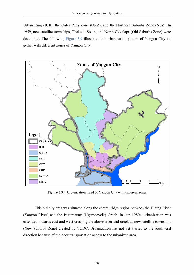
3 Yangon City Water Supply System
28
Urban Ring (IUR), the Outer Ring Zone (ORZ), and the Northern Suburbs Zone (NSZ). In
1959, new satellite townships, Thaketa, South, and North Okkalapa (Old Suburbs Zone) were
developed. The following Figure 3.9 illustrates the urbanization pattern of Yangon City to-
gether with different zones of Yangon City.
Figure 3.9: Urbanization trend of Yangon City with different zones
This old city area was situated along the central ridge region between the Hlaing River
(Yangon River) and the Pazuntaung (Ngamoeyeik) Creek. In late 1980s, urbanization was
extended towards east and west crossing the above river and creek as new satellite townships
(New Suburbs Zone) created by YCDC. Urbanization has not yet started to the southward
direction because of the poor transportation access to the urbanized area.

3 Yangon City Water Supply System
29
Present Land Use 3.1.3.3
In the urban development study for Yangon City, the land use map of Yangon City
was developed based on the analysis of satellite images in 2012 (see in Figure 3.10) (JICA &
YCDC, 2014). According to the land use pattern, most of the outside areas of Yangon City
are still as cultivated land although Yangon City area is undergoing development. The catch-
ment areas of the supply water reservoirs are dense forest, sparse forest and scattered trees
zones.
Figure 3.10: Land use map of Yangon City and its surroundings (2012)
Industrialization 3.1.3.4
Industrialization pattern of Yangon City and surrounding 6 townships are composed of
37% for processing and manufacturing sector, 25% for trade sector, 24% for service sector
and only 8% for the total of agriculture, livestock, and fishery sectors in 2011 (JICA &
YCDC, 2014). According to the data from Yangon regional office of Planning Department,
Ministry of National Planning and Economic Development, Myanmar, the whole Yangon
Region had 15089 factories/workshops in Yangon Region in 2010/11, and about 80% of this
amount (11903 factories/workshops) is in the Yangon City area (JICA & YCDC, 2014). Ac-

3 Yangon City Water Supply System
30
cording to the number of factories, NewSZ is the most industrialized zone and IUR, OldSZ,
and NSZ are industrialized zones. Department of Human Settlement and Housing Develop-
ment (Ministry of Construction) and YCDC implemented 25 industrial zones in Yangon City.
Health 3.1.3.5
The life expectancy at birth of Myanmar is 66 for both sexes, whereas the regional av-
erage is 67, and the global average is 70 (WHO, 2012). Therefore, the life expectancy of My-
anmar is a little bit lower than that of the world average but nearly the same with that of
Southeast Asian countries. Under-5 mortality rate, Infant mortality rate (under 1), Crude
death rate, and life expectancy were improved from 106 in 1990 to 52 in 2012, from 76 in
1990 to 41 in 2012, 10.1 in 1990 to 8.5 in 2012, 58.7 in 1990 to 65 in 2012, respectively
(UNICEF, 2013).
However, Crude birth rate was decreased 26.8 in 1990 to 17.4 in 2012 together with
decreasing fertility rate in Myanmar (UNICEF, 2013). Myanmar has a low fertility rate com-
paring with the other Southeast Asia countries and fertile rate has been declining significantly
from 4.7 in 1983, 2.4 in 2001 to 2 in 2012 (UNICEF, 2013; Jones, 2007). The fertility rate is
mainly lower in urban areas because of extreme delays in marriage and the high number of
single and unmarried women in reproductive age. In Myanmar, the proportion of single wom-
en at age 30-34 increased 9.3% in 1970 to 25.9% in 2000 (Jones, 2007).
3.2 Study Organization Description
This section will describe Yangon City Development Committee (YCDC), the present
city authority, and its department, Engineering Department (Water & Sanitation) which is
responsible for the city’s water supply facility.
3.2.1 Yangon City Development Committee (YCDC)
YCDC was initially established as a city municipal organization since Myanmar was
under the British to carry out municipal works, and its name was changed in history as Ran-
goon City Municipal Corporation in 1922, as Rangoon City Municipal Committee in 1972, as
Rangoon City Development Board in 1977, as Rangoon City Development Committee in
1985 (YCDC, 2014a).

3 Yangon City Water Supply System
31
According to the provisions of Yangon City Development Law (14 May 1990),
YCDC bestowed wide powers and authority, for instance, YCDC was authorized to imple-
ment its own project by using its own funding resources. However, at present, YCDC needs to
apply permissions of projects to the national government, and the funding sources of YCDC
are incorporated into the national budget by the new policy. YCDC set up as a ministerial
level and comprises with 20 departments and one committee office, to create a modern city
with the features and characteristics of city while preserving its greenery and the intrinsic
beauty for its citizens by the guidance of the national government. YCDC is directly respon-
sible for the development and maintenance of Yangon City in all aspects.
According to Yangon City Development Law, YCDC must organize with minimum
seven members to maximum 15 members; the Chairman, Vice-Chairman (Vice-Mayor), Sec-
retary, Joint-Secretary, and the other are Committee Members. Mayor of Yangon City is re-
sponsible not only the Chairman of YCDC but also the minister of Development Affairs of
Yangon Region. The current organizational chart of YCDC is showing in Figure 3.11.
Figure 3.11: Organization chart of Yangon City Development Committee
Committee-7
Mayor
Chairman of YCDC
Minister of Development Affairs
(Yangon Region)
Joint-Secretary
Committee-4 Committee-5 Committee-6
Pollution Control &
Cleansing Department
Engineering Department
(Building)
Inspection
Department
Markets
Department
Security & Disciplinary
Department
Assessor
Department
Revenue
Department
Administration
Department
Engineering Department
(Roads & Bridge)
Playgrounds, Parks &
Gardens Department
Engineering Department
(Water & Sanitation)
Health
Department
Motor Transport &
Workshop Department
Central Stores
Department
Veterinary & Slaughter
Houses Department
Co-ordination
Department
East District Office North District Office West District Office South District Office
Production
Department
Committee Office
Secretary
Budget and Accounts
Department
City Planning and Land
Administration Department
Public Relations and
Information Department
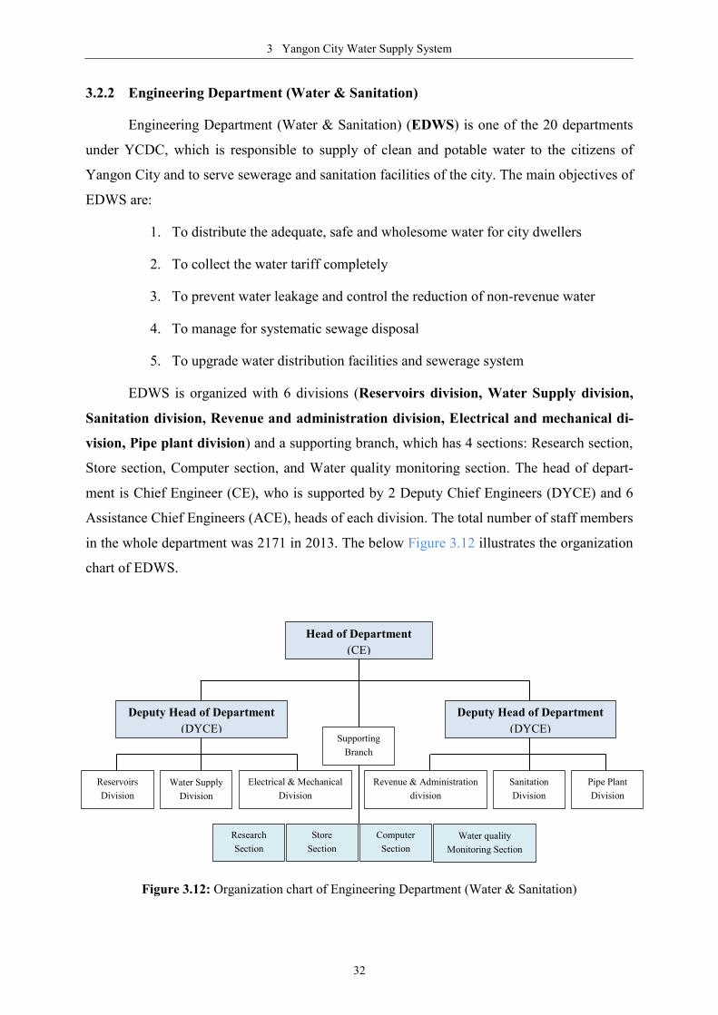
3 Yangon City Water Supply System
32
3.2.2 Engineering Department (Water & Sanitation)
Engineering Department (Water & Sanitation) (EDWS) is one of the 20 departments
under YCDC, which is responsible to supply of clean and potable water to the citizens of
Yangon City and to serve sewerage and sanitation facilities of the city. The main objectives of
EDWS are:
1. To distribute the adequate, safe and wholesome water for city dwellers
2. To collect the water tariff completely
3. To prevent water leakage and control the reduction of non-revenue water
4. To manage for systematic sewage disposal
5. To upgrade water distribution facilities and sewerage system
EDWS is organized with 6 divisions (Reservoirs division, Water Supply division,
Sanitation division, Revenue and administration division, Electrical and mechanical di-
vision, Pipe plant division) and a supporting branch, which has 4 sections: Research section,
Store section, Computer section, and Water quality monitoring section. The head of depart-
ment is Chief Engineer (CE), who is supported by 2 Deputy Chief Engineers (DYCE) and 6
Assistance Chief Engineers (ACE), heads of each division. The total number of staff members
in the whole department was 2171 in 2013. The below Figure 3.12 illustrates the organization
chart of EDWS.
Figure 3.12: Organization chart of Engineering Department (Water & Sanitation)
Head of Department
(CE)
Water Supply
Division
Reservoirs
Division
Revenue & Administration
division
Deputy Head of Department
(DYCE)
Deputy Head of Department
(DYCE)
Electrical & Mechanical
Division
Sanitation
Division
Pipe Plant
Division
Store
Section
Supporting
Branch
Water quality
Monitoring Section
Computer
Section
Research
Section

3 Yangon City Water Supply System
33
3.3 History and Status quo of Water Supply System
This section will present two parts of Water supply system of Yangon City. The first
part deals with the water supply system history in the past and the second part deals with the
present water supply system.
3.3.1 Past Water Supply System
Yangon city water supply system has a long history of more than 150 years. In 1842,
King Tharrawady gave instruction to construct 30 open wells in Yangon City to start the wa-
ter supply facility of the city.
In 1879, the first water supply system with pipeline was initiated in Yangon City by
using water from Kandawgyi Lake to Baotahtaung and Pazundaung townships via 10" diame-
ter cast iron pipes.
In 1884, this water supply system was augmented by the construction of Inya Lake,
water from which was diverted to Kandawgyi Lake by 30" diameter pipelines and distributed
to the city through 27" diameter pipelines.
In 1894, the water supply system in Yangon City was developed with pumping station
and service water tank by the construction of Phoesein pumping station and Shwedagon ser-
vice water tank (1MG storage capacity). The water delivered from Kandawgyi Lake to Phoe-
sein pumping station was pumped to the Shwedagon service tank via 27" diameter pipeline
and distributed water to the western part of the city from that tank.
In 1904, Hlawga Reservoir (14 MGD supply capacity), situated about 17 miles
(27km) north of Yangon City, was introduced in Yangon City water supply system, continu-
ously, the water supply from Kandawgyi Lake and Inya Lake has ceased due to the deteriora-
tion of water quality from these lakes resulted by rapid urbanization. Water from Hlawga res-
ervoir was pumped through 42" diameter CI pipeline to Yegu pumping station by booster
pumping station of Hlawga reservoir. In 1906, the construction of Yegu pumping station was
completed, and water was pumped to Shwedagon reservoir via 42" diameter, from which wa-
ter was distributed to the whole city. Since that time, the use of Phoesein pumping station was
terminated. In 1925, Kokkine service water tank (20 MG storage capacity) was constructed
and added to the existing water supply system to expand the served area.

3 Yangon City Water Supply System
34
In 1941, the construction of Gyobyu reservoir (27 MGD supply capacity), situated
about 40miles (64km) north of the city, was completed, and water was supplied with 56" di-
ameter mild steel pipes through Yegu pumping station to Kokkine service water tank.
In 1989, Phugyi reservoir (54 MGD supply capacity), situated about 32 miles (51
km) of the city, was added to the water supply system by connecting with Hlawga reservoir
through a 60" diameter pre-stressed concrete pipe. In 1992, 66" diameter pre-stressed concrete
pipe laying project from Hlawga reservoir to Yegu pumping station was completed and water
has been distributed to Yangon City. At that time, the daily water supply amount of the whole
system was 85 MGD, including water amount (10MGD) from YCDC owned tube wells.
In 2000, Yangon Pauk ground water treatment project was implemented to supply
1MGD water amount to Dala Township, southern part of the city on the other bank of Yangon
River.
In 2005, Ngamoeyeik WTP project (Phase 1 with 45 MGD supply capacity), using
water source from Ngamoeyeik reservoir, which was constructed and managed by Ministry
of Agriculture and Irrigation, was operated to supply water to the eastern part of the city, es-
pecially, new suburb townships of the city.
In 2009, South Dagon ground water treatment project (No.1 and No.2 with total 2
MGD supply capacity) and Thaephyu ground water treatment project (1MG supply capacity)
was implemented at the eastern and western extended part of the city to supply water to the
suburb regions which are far from the main water supply system.
The second phase of Ngamoeyeik WTP was accomplished in early 2014, and it started
its function to reinforce the water supply system of the city with daily supply capacity 45 MG.
3.3.2 Present Water Supply System
Water Supply Sources 3.3.2.1
The current water supply amount of YCWSS is 205 MGD, including the amount of
water generated from the second phase of Ngamoeyeik WTP, i.e. 45MGD. The total water
supply amount was 160 MGD until the end of financial year 2013-2014.
Table 3.2 shows a list of current water sources of Yangon City together with their dai-
ly water supply capacity. About 90% of the water source of the system is surface water from
reservoirs, and the rest is ground water from tube wells as the supplement of water supply
system.

3 Yangon City Water Supply System
35
Table 3.2: Current water sources of Yangon City Water Supply System
Water Sources Daily Capacity Water Source Start-up Year
Hlawga Reservoir 14 MGD Surface water 1904
Gyobyu Reservoir 27 MGD Surface water 1940
Phugyi Reservoir 54 MGD Surface water 1992
Ngamoeyeik WTP (Phase 1) 45 MGD Surface water 2005
Ngamoeyeik WTP (Phase 2) 45 MGD Surface water 2014
Yangon Pauk 1 MGD Ground water 2000
South Dagon 2 MGD Ground Water 2009
Thaephyu 1 MGD Ground Water 2009
YCDC tube wells 16 MGD Ground water -
Total 205 MGD 90% Surface Water + 10% Ground Water
Table 3.3: Reservoirs of Yangon City Water Supply System
Items Hlawga
Reservoir
Gyobyu
Reservoir
Phugyi
Reservoir
Ngamoeyeik
Reservoir
Constructed years 1900-1904 1937-1940 1973-1984 1992-1995
Location (from city) 17 mi North 40 mi North 32 mi North 38 mi North
Catchment area (sq-mi) 10.5 12.9 27.27 160
Water surface area (sq-mi) 4.4 2.8 6.8 17.19
Total capacity (MG) 12000 16600 23000 52000
Effective capacity 10000 8240 20000 48840
Maximum Water Level 62 215 120.86 117
Top of spillway (ft) 62 215 115.5 107
1st
intake level (ft) 57.2 201 90 90
2nd
intake level (ft) 49.2 180 74 72
3rd
intake level (ft) 42.2 138 - -
Water supply capacity (MGD) 14 27 54 45 + 45
Start-up year 1904 1940 1992 2005 (Phase-1)
2014 (Phase-2)
Table 3.3 lists the physical and operational data of reservoirs used in YCWSS. YCDC
owns three water supply reservoirs, namely, Hlawga, Gyobyu, and Phugyi, and operates and
manages these reservoirs only for city water supply purpose. Ministry of Agriculture and Irri-
gation (MoAI) has constructed and managed Ngamoeyeik reservoir for multi-purposes, such
as water supply for agriculture, saltwater intrusion prevention, flood control etc., and one of
these purposes is to supply 90 MGD raw water for Yangon City. YCDC constructed Nga-
moeyeik WTP for the treatment of raw water obtained from Ngamoeyeik reservoir. First
phase of WTP has been operated in 2005 and second phase in 2014 (March), and each phase
has capacity of 45 MGD.
YCDC has three main ground water supply projects in NewSZ and SCBD, which are
far from the main water supply network. Moreover, YCDC is using ground water source from

3 Yangon City Water Supply System
36
tube wells and directly injected into the distribution pipeline network to reinforce the surface
water from reservoirs. At present, there are 645 YCDC-owned tube wells with total maximum
yield amount of 20 MGD, however actual yield amount is less that maximum amount is de-
pending on the operation hours of the tube wells. Most of the tube wells are concentrated in
the CBD area. Moreover, about 3 million populations in Yangon City, who cannot get
YCWSS services, are using private tube wells as a water source. The total withdrawal amount
from both YCDC and private tube wells is estimated about 79MGD. If additional groundwa-
ter would be used in future to meet the increasing water demand, this extraction amount can
exceed the total groundwater potential, i.e. 83 MGD (estimated).
Water Supply Facilities
There are six WTPs in the existing YCWSS. Two treatment plants are for the surface
water treatment and treated by flocculation, sedimentation, and filtration processes. The other
four are ground water treatment plants by cascade aeration and filtration processes. In
YCWSS, there are six main pumping stations to transport water and to supply water with
pressure, however, most of the pumping stations require proper equipment for operation, such
as pressure gauges, flow meters etc. YCWSS has two service water tanks to regulate the water
supply.
Water Supply Pipelines
In YCWSS, some transmission pipelines are more than 100 year old and choked by
scaling. Also, the distribution network have been expanded year by year due to population
growth in the city and development activities, thus, new and old pipe are mixed. The total
length of transmission and distribution pipes in YCWSS is about 1455 km and the detail data
of aged pipes are listed in Table 3.4.
Table 3.4: Aged transmission main pipes in YCWSS
Start-up year Pipe material Diameter Length Age
1904 Cast iron 1060 mm 22.85 km 109
1914 Mild steel 1060 mm 8.05 km 99
1940 Mild Steel 1400 mm 69.2 km 73
1989 Pre-stressed concrete 1520 mm 25.75 km 24
1992 Pre-stressed concrete 1650 mm 16.74 km 21
The following Figure 3.13 illustrates the current water supply system of Yangon City
together with water supply service facilities, such as reservoirs, treatment plant, pumping sta-
tions, main transmission pipeline, etc.

3 Yangon City Water Supply System
37
Figure 3.13: Current Water Supply System of Yangon City in 2013 (JICA & YCDC, 2014)

3 Yangon City Water Supply System
38
Demand sites 3.3.2.2
The main objective of the whole system is to supply the adequate safe water for the
city, so the main and only one demand site in this system is Yangon City, with population
5.14 million in 2013. According to the data of EDWS, the daily water consumption amount
for a person in Yangon City is about 30 imperial gallons.
In 2013, the total daily water demand was 154.2 MGD by using the consumption rate
30gpcd (gallons per capita day).
Demand coverage
The water demand coverage of the YCWSS is about 30 % and people with no water
supply service obtain water from other water sources like wells, tube wells, ponds, and rain
(Yangon Region Government, YCDC & JICA, 2013; Khaing, 2006). Generally, Yangon City
Water Supply System can supply water only one-third of city dwellers.
There were 825620 households in Yangon City, however, the number of water con-
nections, households connected with city water supply system, was only 269268 at the end of
2013. Based on the number connection, the water demand coverage of Yangon City was
about 32 %.
In 2013, the actual daily water supply amount in Yangon City was 54.52 MGD that
was calculated by using the actual income from 2013-December water meter bills. The total
daily water demand was 154.2 MGD calculated by using water consumption rate 30 gpcd for
5.14 million populations in 2013. Therefore, the water demand coverage of Yangon city in
December 2013 was about 35% according to the income based calculation. The following
Table 3.5 shows the calculations of demand coverage of the system in Yangon City based on
connections and volume derived from actual income. In 2013, the average water supply vol-
ume was about 50 MGD and the demand coverage is about 32.4 % for the whole year.
Table 3.5: Demand coverage of the YCWSS in 2013
Demand site Yangon City
Daily Demand 154.2 MGD 5.14 million population with 30 gpcd consumption
Demand
Coverage
(connection based)
32.6 % The ratio of the number of actual supply connection, i.e. 269268,
and the number of households, i.e. 825620
Demand
Coverage
(income based)
35%
The ratio of the actual supply volume derived from actual in-
come, i.e. 54.52 MGD, and the total demand by using 30 gpcd,
i.e. 154.2 MGD
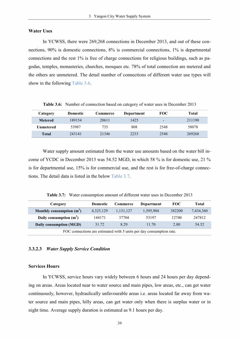
3 Yangon City Water Supply System
39
Water Uses
In YCWSS, there were 269,268 connections in December 2013, and out of these con-
nections, 90% is domestic connections, 8% is commercial connections, 1% is departmental
connections and the rest 1% is free of charge connections for religious buildings, such as pa-
godas, temples, monasteries, churches, mosques etc. 78% of total connection are metered and
the others are unmetered. The detail number of connections of different water use types will
show in the following Table 3.6.
Table 3.6: Number of connection based on category of water uses in December 2013
Category Domestic Commerce Department FOC Total
Metered 189154 20611 1425 - 211190
Unmetered 53987 735 808 2548 58078
Total 243141 21346 2233 2548 269268
Water supply amount estimated from the water use amounts based on the water bill in-
come of YCDC in December 2013 was 54.52 MGD, in which 58 % is for domestic use, 21 %
is for departmental use, 15% is for commercial use, and the rest is for free-of-charge connec-
tions. The detail data is listed in the below Table 3.7.
Table 3.7: Water consumption amount of different water uses in December 2013
Category Domestic Commerce Department FOC Total
Monthly consumption (m3) 4,325,129 1,131,127 1,595,904 382200 7,434,360
Daily consumption (m3) 144171 37704 53197 12740 247812
Daily consumption (MGD) 31.72 8.29 11.70 2.80 54.52
FOC connections are estimated with 5 units per day consumption rate.
Water Supply Service Condition 3.3.2.3
Services Hours
In YCWSS, service hours vary widely between 6 hours and 24 hours per day depend-
ing on areas. Areas located near to water source and main pipes, low areas, etc., can get water
continuously, however, hydraulically unfavourable areas i.e. areas located far away from wa-
ter source and main pipes, hilly areas, can get water only when there is surplus water or in
night time. Average supply duration is estimated as 9.1 hours per day.

3 Yangon City Water Supply System
40
Water pressure
Water pressure of YCWSS also has the same situation as service hours’ case and var-
ies widely from < 0.3 bar to >1.5 bars, and average pressure is about 0.75 bars. Hydraulically
favourable areas get high pressure, while hydraulically unfavourable areas get low pressure.
Non-Revenue Water Rate
Previously revenue water quantity was estimated as 54.52 MGD while supplied quan-
tity was estimated as 160 MGD. Non-revenue water is calculated as 105.48 MGD or 66 %
and the detailed water balancing analysis for non-revenue water amount is shown in Table
3.8. Non-revenue water amount in YCWSS is high because of leakage in old pipes, free water
supply to religious buildings, water meters malfunction and illegal connections.
Table 3.8: Non-revenue water analysis of YCWSS
Total water
supply volume
160 MGD
(100%)
Authorized
water
consumption
Billed authorized consumption
54.52 MGD
(34%)
Revenue water
Unbilled authorized consumption
105.48 MGD
(66%)
Non-revenue
water
Water losses
Commercial losses
Unauthorized consumption
Meter inaccuracies
Data handling errors
Physical losses (50% estimated)
Leakage in water facilities
Leakage in pipelines
Leakage in meters & connections
Water billing system
In YCWSS, metered connections are charged by fixed rate per unit billing system in
every month, and unmetered connections are charged by flat rate billing system in every quar-
ter of the year, i.e. every three months. Even though customers can be categorized in to four
types: domestic, commerce, department, and FOC, there are only two charged rates, i.e. 0.085
€ (110 MMK) per m3 for commercial connections and 0.068 € (88 MMK) per m
3 for other
connections except FOC connections. Flat rate billing system is charged depending on the
estimated monthly water consumption.

3 Yangon City Water Supply System
41
Problems in YCWSS 3.3.2.4
Various problems, relating with technology, organization, institution, and finance &
management that are encountering in YCWSS are listed in the following Table 3.9.
Table 3.9: Major problems facing in YCWSS
Technical problems
(1) Low demand coverage
(2) High non-revenue water amount
(3) Poor water quality
(4) Ageing water facilities and main pipelines
(5) Inappropriate layout of facilities
(6) Insufficient O&M of facilities
Organizational problems
(1) Lack of planning section
(2) Lack of monitoring section
(3) Lack of O&M and management according to PIs
(4) Poor awareness of customer services
(5) Poor water quality testing system
(6) Poor human resources development in the organization
Institutional problems
(1) Standards for installation of service connections
(2) Standards for water meter
(3) Standards for installation of individual storage tank
(4) Standards for installation of individual pumping facilities
(5) Inspection of installation works for service pipe
Financial Management prob-
lems
(1) Cheap water price
(2) Water pricing system
(3) Need for introducing corporate accounting system
(4) Budget with little freedom
(5) Computerization in limited services
Consumer Survey 3.3.2.5
In the Project for the Strategic Urban Development Plan of the Greater Yangon
(2012), the household survey was carried out in every township with the total 10,000 house-
holds sample, i.e. 1 % of each township’s households (JICA & YCDC, 2014). The question-
naires related to water are regarding about water source, access to water and consumption,
evaluation of existing service level and water-borne diseases (see details in Appendix A). The
following results were obtained from this survey.
Major Water Source
The water source for various purposes except drinking purpose is private tube well
(37%), followed by YCWSS piped water (34 %) and neighbour’s well (9 %). This 34 % of
YCWSS piped water is equivalent to the coverage of water supply system.

3 Yangon City Water Supply System
42
The main sources of drinking water are bottled water (45 %), private tube well (17 %),
and YCWSS piped water (12 %).
Desirable Water Amount
About 74 % of the respondents answered that they satisfied with the current consump-
tion amount i.e. 30 gpcd, and 11% wanted to consume two times of the current consumption.
Expenditure for Water
The average expenditure of a household for drinking water is about 4.3 € (5600
MMK) per month and 3.4 € (4400 MMK) for other use. Some respondents answered high
expenditure, so that the mean is higher than the median. The median shows 1 € (1300 MMK)
for drinking water and 0.55 € (700 MMK) for other use, so it is estimated that the general
public spends 1.55 € (2000 MMK) per month for water supply.
Willingness to Pay for Water Supply Services
The question on their willingness to pay for drinkable water supply 24-hour services
was asked of all respondents. For untreated water supply, 54 % answered less than 0.8 €
(1000 MMK) per month, and for a drinkable water supply, 44 % answered less than 0.8 € per
month. The average willingness to pay the amount was 1.88 € (2400 MMK) per household
per month and the monthly average water-consumption per household was also estimated
13.9 m3. Therefore, the average willingness to pay per cubic meters was estimated as 0.135 €
(175 MMK). If this amount is compared to the current tariff rate for domestic use, which is
0.068 € (88 MMK), the current tariff rate is almost half time lower than the willingness to pay
the amount.
Focusing on the relationship between willingness to pay and monthly household in-
come, the willingness to pay the amount per month is equivalent to 1.4% of the monthly me-
dian household income, i.e. 135 € (177500 MMK). Therefore, it is less than 4% of the income
that is considered as a typical benchmark parameter.
As a result, the current tariff rate level and a willingness to pay rate are relatively low.
If it is assumed that the affordability to pay is 4% of monthly average household income, the
affordability to pay for water supply services is 0.385 € (500 MMK) per m3.
Waterborne Diseases
1.4 % of the respondents’ household members suffered from the diarrhoea, and other
diseases such as dysentery, Cholera and typhoid are low (0.1 ~ 0.6 %). The percent for one-
time infection in a year is 50.6 %, and 2-5 times is 45.6 %.

3 Yangon City Water Supply System
43
Satisfaction of YCWSS Service
According to the Household Survey, the degree of satisfaction on YCWSS is lower
than that on other sources. This means that YCWSS cannot supply an adequate amount of
safe drinking water to the customers continuously due to the limited amount of water source
and inadequate capacity of water supply facilities.
Service level target for future 3.3.2.6
In the project for the improvement of YCWSS, the service level targets for the per-
formance indicators (PIs) are set for the future (in Table 3.10).
Table 3.10: Service level target of YCWSS (JICA & YCDC, 2014)
PIs Target Year
2013 2018 2020 2025 2030 2035 2040
Non-revenue water (%) 66 51 46 35 26 20 15
Leakage rate (%) 50 37 33 25 18 13 10
Demand coverage (%) 35 45 50 60 65 70 80
Served population (million) 1.8 2.6 3.0 4.1 5.1 6.2 8.0
Water consumption (gpcd) 30 30 30 35 35 35 40
Supply Pressure (bar) 0.75 > 1.5
Supply duration (hour) 8hrs. 24hrs.
Water quality Non-
drinkable Drinkable
To achieve these targets and to meet the increased water demand, the future manage-
ment plan for water supply sources of YCWSS is implemented. According to this plan,
groundwater abstraction in Yangon City need to be gradually reduced, and not utilized after
2025 to prevent groundwater table lowering, saline water intrusion, and land subsidence oc-
curring. In addition, alternative water sources, such as river water sources, are deciding to
implement for future demand. The proposed future development projects are listed in the be-
low Table 3.11. According to the feasibility study for these projects, the data of potential riv-
ers, which are estimated by using the data of MoAI reports (see in Appendices), are about
9984 MGD in Kokkowa River and 23424 MGD in Toe River and that potential water source
amount is much higher than the withdrawal amount of the respective projects which is 240
MGD in Kokkowa River project and 180 MGD in Toe River project.

3 Yangon City Water Supply System
44
Table 3.11: Proposed future development projects of YCWSS (JICA & YCDC, 2014)
Project
Start-up year & Water supply capacity
2018 2020 2025 2030 2035 2040
Lagunpyin Reservoir (40 MGD) 40MGD - - - - -
Kokkowa River (240 MGD) - 15MGD 45MGD 60MGD 120MGD -
Toe River (180 MGD) - - 15MGD 15MGD 30MGD 120MGD
Total 40MGD 15MGD 60MGD 75MGD 150MGD 120MGD
Moreover, other management plans for the improvement of YCWSS will be estab-
lished not only to increase the water supply but also to control the water demand. For exam-
ple, non-revenue water control management plan, water billing system management plan,
human resources development plan, etc.

4 Development of WEAP model for YCWSS
45
4 Development of WEAP model for YCWSS
This part will describe the development of WEAP model for YCWSS. In order that the
water supply in the future is sustainable and adequate in quality and quantity to meet the
booming demand, WEAP model will be developed and applied to evaluate the existing
YCWSS and expected future scenarios for YCWSS by taking into account the different fac-
tors and policies that may affect demand and supply sources.
WEAP is a practical tool for water resources planning which incorporates not only wa-
ter supply-side and water demand-side issues, but also water quality and ecosystem preserva-
tion issues, by its integrated approach to simulate water systems and by its policy orientation
(SEI, 2011). This model will simulate water supply system operation of the city on a user-
defined time step; compute the water mass balance for all nodes and lines of WEAP, compo-
nents of the water system and links of these components, for the simulation period; evaluate
and forecast water development and management scenarios for the future (SEI, 2011; Hamlat
et al., 2013). The results coming out from WEAP software can assist planners and water sup-
ply authorities in developing recommendation for future water supply and demand manage-
ment. In this study, WEAP model is selected to use as a database tool, a forecasting tool, and
a policy analysis tool to analyse about YCWSS to forecast for the future options.
Application of the WEAP model generally includes the following steps (SEI, 2011).
Setting up the Study Definition, which includes the spatial boundary, the time frame,
the system components, and the configuration of the problem
Entering data in the Current Accounts, which provides an overview of the actual
situation of the system (water demand, supply resources, pollution loads), and can also
be viewed as a calibration step in the development of an application
Creating Key assumptions in the Current Accounts, if necessary, which represent pol-
icies, costs and factors that affect demand, pollution, supply, and hydrology
Building Scenarios on the Current Accounts, which can be explored the impacts of al-
ternatives on the future water supply and demand
Evaluating Scenarios, regarding with water demand coverage, costs, compatibility
with environmental targets, sensitivity to uncertainty
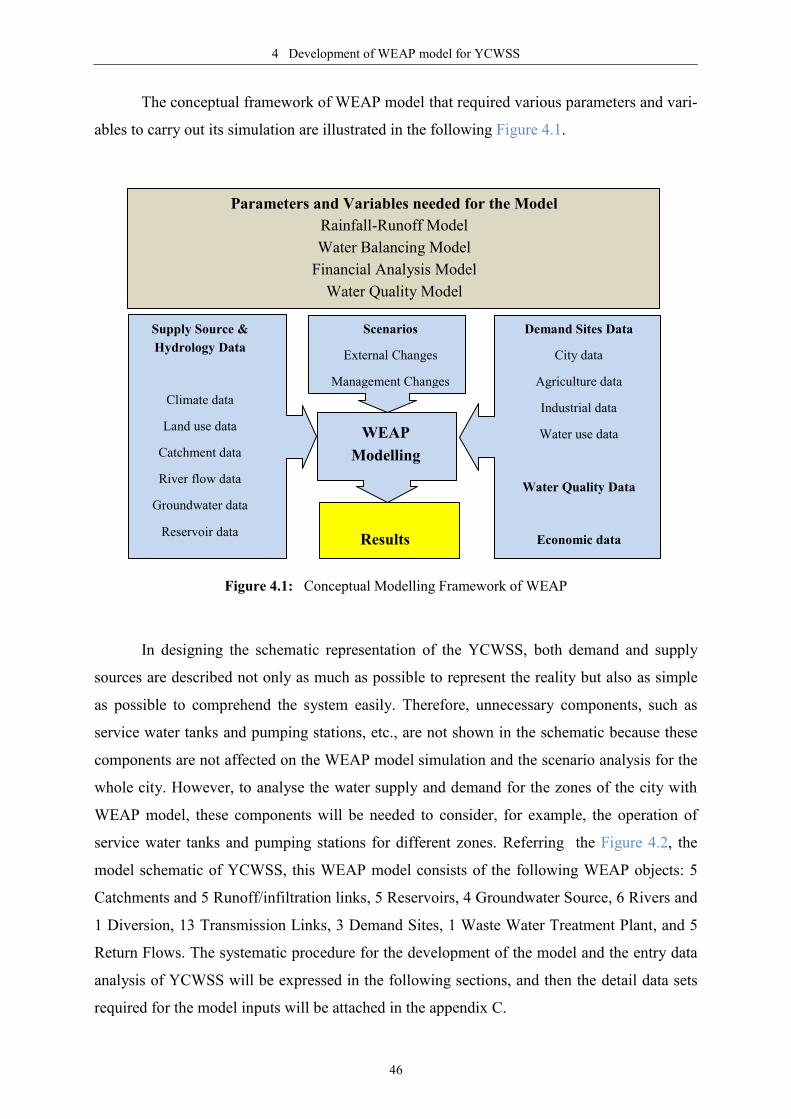
4 Development of WEAP model for YCWSS
46
The conceptual framework of WEAP model that required various parameters and vari-
ables to carry out its simulation are illustrated in the following Figure 4.1.
Figure 4.1: Conceptual Modelling Framework of WEAP
In designing the schematic representation of the YCWSS, both demand and supply
sources are described not only as much as possible to represent the reality but also as simple
as possible to comprehend the system easily. Therefore, unnecessary components, such as
service water tanks and pumping stations, etc., are not shown in the schematic because these
components are not affected on the WEAP model simulation and the scenario analysis for the
whole city. However, to analyse the water supply and demand for the zones of the city with
WEAP model, these components will be needed to consider, for example, the operation of
service water tanks and pumping stations for different zones. Referring the Figure 4.2, the
model schematic of YCWSS, this WEAP model consists of the following WEAP objects: 5
Catchments and 5 Runoff/infiltration links, 5 Reservoirs, 4 Groundwater Source, 6 Rivers and
1 Diversion, 13 Transmission Links, 3 Demand Sites, 1 Waste Water Treatment Plant, and 5
Return Flows. The systematic procedure for the development of the model and the entry data
analysis of YCWSS will be expressed in the following sections, and then the detail data sets
required for the model inputs will be attached in the appendix C.
Supply Source &
Hydrology Data
Climate data
Land use data
Catchment data
River flow data
Groundwater data
Reservoir data
Scenarios
External Changes
Management Changes
WEAP
Modelling
Demand Sites Data
City data
Agriculture data
Industrial data
Water use data
Water Quality Data
Economic data Results
Parameters and Variables needed for the Model
Rainfall-Runoff Model
Water Balancing Model
Financial Analysis Model
Water Quality Model

4 Development of WEAP model for YCWSS
47
Figure 4.2: Simplified schematic for WEAP model of YCWSS
Legend
River
Diversion
Reservoir
Groundwater
Other Supply
Demand Site
Catchment
Runoff/Infiltration
Transmission Links
Wastewater Treatment Plant
Return Flow
Future Projects

4 Development of WEAP model for YCWSS
48
4.1 Study Definition
In developing a WEAP model, the study boundary, the study period, and the compo-
nents of the study system are necessary to define as a self-contained set of data and assump-
tions. The study area can be defined as a specific water supply system, such as a river basin or
a groundwater aquifer, or political or geographic boundaries (SEI, 2011).
The spatial boundary of the study area for YCWSS is initially created in WEAP by us-
ing the built-in GIS-based layers (Ocean, Country, States, Cities, and Major Rivers), and also
by adding external raster layers (Geo TIFF or ArcView GRID files) and vector layers (ESRI
Shape files) to orient and construct the system easily and to comprehend the system situation
clearly. In this model, a raster layer is added as a background map, and other vector layers,
such as Myanmar administrative areas, Myanmar water lines, Myanmar water areas, City ar-
ea, Land use, Hydro features, Elevations, Reservoirs, are added to assist the model develop-
ment and the results presentation. These added vector and raster layers are needed to adapt the
geographic coordinate system with WEAP, which is WGS84, un-projected and directly based
on latitude and longitude (SEI, 2011).
After creating the study area, the study period for the model is needed to define. For
this model, the Current Accounts Year is set as 2013 and the Last Year of Scenarios is set as
2040. The Time Steps per year is used as 12 based on a calendar month by starting in Janu-
ary and adding leap days. The Current Accounts Year is chosen to work as the base year of
the model, and all system information, such as demand and supply data, on this year is input
into the Current Accounts. Scenarios are built based on the data set of the Current Accounts
and are explored for the possible changes to the system in the future until the last year of sce-
narios. A more detailed discussion of scenarios will be presented in Section 5.
The units of parameters, the water quality constituent parameters, and the basic pa-
rameters of the model can be predefined in WEAP. In this YCWSS model, most of the units
are used in the British System, which is the local unit system in Myanmar (e.g. Imperial gal-
lons for water volume, feet for length, squared miles for area), and the required unit conver-
sions from the local system to the global system, SI system, are listed at the first part of this
thesis. In this study, the water quality modelling will not carry out due to the insufficient data.
In this model, different demand site components can have different monthly variation, and
different supply site components can have different climate data.
In WEAP, the system components, such as Catchments, Rivers, Reservoir, Groundwa-
ter, Demand Site, Catchment, Runoff/infiltration, Transmission Link etc., can be defined by

4 Development of WEAP model for YCWSS
49
using its drag and drop graphical interface to describe and visualize the configuration of the
water supply and demand system and its physical features. As it has been mentioned as be-
fore, the model for YCWSS is described as simple as possible to easily understand the sys-
tem, by using current water supply sources (surface water from reservoirs and ground water
from tube wells), future supply projects (river water from rivers), transmission pipelines from
the supply source to demand sites. Yangon City is represented as only one demand site with
aggregate method because this study is aimed to represent the supply-demand situation of the
city level, and the acquired data is not sufficient to disaggregate the Yangon City. However,
there are three demand sites in this model; one is Yangon City, and the other two are Nga-
moeyeik WTP and Yegu pumping station to represent the some losses in these facilities. Nev-
ertheless, the water from these facilities is transmitted to the Yangon City demand site in the
end. In WEAP, nodes represent physical components of the system, and lines, which repre-
sent the transmission components of the system, link these nodes. Each node that represents
the supply components may have a start-up year, and before this year, it cannot be active.
Therefore, this feature can use to represent the component that will be implemented after the
Current Accounts as future projects.
After the schematic of the system has been implemented, the required data for each
component of the system must be inserted in the Current Accounts to stand for the actual situ-
ation of the system in current condition.
4.2 Data Entry in the Current Accounts
In WEAP, the data can enter either putting numerals directly or using WEAP data en-
try wizards, such as Expression Builder or Time-Series Wizard or ReadFromFile Wizard
or Lookup Function Wizard (SEI, 2011). The data for demand sites and catchments, sup-
ply and resources, hydrology, water quality, key assumptions and other assumptions are
needed to input under the Current accounts to represent the current state of the water supply-
demand system. In scenarios analysis, the alternatives data are necessary to modify under the
respective scenarios to analyse the impacts of these alternatives in the future water supply-
demand.
The data entry for the Current Accounts (2013) of YCWSS model will be explained
precisely in the following sub-sections and that for the Scenarios (2014-2040) will be de-
scribed in the next section - Creation of Scenarios in YCWSS-WEAP model.

4 Development of WEAP model for YCWSS
50
4.2.1 Demand Sites and Catchments
The demand sites in WEAP determines the total water amount that required to supply
from the sources and the catchments in WEAP carries out rainfall-runoff analysis in a specif-
ic area and transmits runoff water to the other water facilities such as reservoirs, rivers, and
infiltrated water to groundwater aquifers by balancing water inputs and outputs (SEI, 2011).
Demand sites 4.2.1.1
Demand site can be defined as a set of water users sharing a physical distribution sys-
tem or an important withdrawal supply source in a defined region (SEI, 2011). Demand sites
can be lumped together into aggregate demand sites or demand sites for different water uses
can be disaggregated into individual demand sites, and this aggregation level is generally de-
termined by the level of detail for water use data available and the level of detail desired for
analysis (SEI, 2011). In this study, the demand data cannot be available for individual sites of
Yangon City, that means the detail data for differ water uses (industrial or domestic etc.) and
different zones of Yangon City, but can be available for the whole city, moreover, the level
aimed to analyse for this master thesis is the whole city level.
Defining demand sites can be used not only for the actual water uses, such as city and
agriculture, but also for the other physical infrastructure, such as pumping stations, withdraw-
al facilities, water treatment plants and well fields (SEI, 2011). Demand sites in WEAP can be
defined according to the following groupings, as major cities or counties, individual user that
manages a water withdrawal point, irrigation sites, demands which return to a wastewater
treatment plant, water utilities (SEI, 2011). In this YCWSS model, Ngamoeyeik water treat-
ment plant, and Yegu pumping station also take into consideration as demand sites together
with the Yangon City, a major demand site for this study. For determining the water demand
for these demand sites, annual demand with monthly variation method is used in this
model. Therefore, the input requirements for demand sites under this method are water use
data, such as annual activity level, annual water use rate, monthly variation, consumption,
loss and reuse data, demand management data, and demand priority.
Water demand is calculated by multiplying the activity level, a measure of social and
economic activity such as population or households for city and hectares for agriculture area,
with the water use rate (SEI, 2011). The water use data of all demand sites in YCWSS model
are listed in Table 4.1. Monthly variation for water consumption of Yegu PS and Nga-
moeyeik WTP is used based on the proportions of the number of days in a month, however

4 Development of WEAP model for YCWSS
51
the actual monthly variation of the consumption for Yangon City is calculated by deriving
from the actual monthly income of water meter bill of EDWS for the period of 2007 to 2013.
This calculation for monthly variation cannot derive directly from monthly income because of
different connection number in different months and the water unit-price changes in the study
period, thus, unit consumption variation in a connection is used in this study. Firstly, the total
actual monthly income is converted into the monthly water charge amount per connection by
using total connection number in the respective month. Then, that monthly water charge
amount per connection is converted again into the monthly consumption unit per connection
by using the water price per unit. At last, the monthly variation percent is calculated by find-
ing the proportion of monthly consumption unit in total annual consumption unit. Consump-
tions for the demand sites are a fraction of their inflows, which represent the water losses to
evaporation or treatment or unaccounted amount for, and these amounts are lost from the sys-
tem (SEI, 2011). According to the data from the water balance research in Germany, the actu-
al consumption amount of urban areas is only 16% of the total inflow and the rest 84% is the
return flow to the environment. So, in this study, the consumption of the Yangon City is used
as 16%, whereas that for Yegu PS is used as 8% and for Ngamoeyeik WTP is 16% depending
on their structure types, Yegu PS is a closed-type system and Ngamoeyeik WTP is an open-
type system.
Loss Rate is the distribution losses in a demand site and otherwise unaccounted for
demands, such as physical leakage in municipal systems, unmetered water use in public parks
and buildings, illegal connections, water used for line flushing, water use for firefighting etc.,
but it should not include transmission losses and should not be confused with Consumption
(SEI, 2011). Consumption is lost from the system and can reduce the return flow, whereas
Loss Rate is not lost from the system but can increase the supply requirements (SEI, 2011).
Reuse Rate is water recycling or reuse to refer the processes in which water is used more
than one application before discharge, and it reduces the supply requirement (SEI, 2011). In
this YCWSS model, all losses from the whole system, i.e. NRW amount 66%, will represent
with transmission losses in transmission links because of the lack of data for different losses.
According to this assumption, there will be input as no loss rate and reuse rate in all demand
sites of YCWSS.
DSM savings (Demand site management savings) represent the percent of reduction
from the total monthly demand due to the various demand-side management strategies, for
example, using water saving technology, using the block-rate water pricing (SEI, 2011). In
this study, this function will use in scenarios analysis.

4 Development of WEAP model for YCWSS
52
Priority is the demand site's priority for supply, relative to all other demands in the
system and represent with integers, 1 is highest priority and 99 is lowest, and this user-defined
demand priority system determines the order of allocations to demand sites (SEI, 2011). The
main objective of this system is to supply adequate water to Yangon City. Thus, the priorities
of all demand sites are used as 1.
Table 4.1: Demand sites data of YCWSS-WEAP model
Demand Sites Yangon City Yegu PS Ngamoeyeik WTP
Annual Activity Level 5142128 cap 1 unit 1 unit
(Water Use Rate) (30gpcd) (95 MGD) (45 MGD)
Annual Water Use Rate 10950 g/person 34675 MG 16425 MG
Monthly Variation (%) Actual water use monthly
variation (2007-2013)
Proportion of
number of days in the month
Consumption (%) 16% 8% 16%
Loss Rate Assumed no loss
Reuse Rate No reuse
DSM savings No demand site management plan
Priority First priority (taken as 1)
Catchments 4.2.1.2
Catchment is a user-defined area for hydrological processes such as precipitation,
evapotranspiration, runoff, irrigation, and yields on agricultural and non-agricultural land
(SEI, 2011). For a catchment, one of four methods, Irrigation Demands Only (Simplified
Coefficient Method), Rainfall-Runoff (Simplified Coefficient Method), Soil Moisture
Method, and MABIA Method (FAO 56, dual Kc, Daily), needs to choose to simulate
catchment processes such as evapotranspiration, runoff, infiltration and irrigation demands,
depending on the data availability and the required level to represent the catchment processes
(SEI, 2011).
In this YCWSS model, there are five catchments, such as Gyobyu, Phugyi, Hlawga,
Ngamoeyeik and Lagunpyin (Start-up year 2015), for the respective reservoirs, and Rainfall
Runoff (simplified coefficient method) is used for the determining the runoff from these
catchments to the reservoirs. This method determines the evapotranspiration using crop coef-
ficients and the remainder of rainfall not consumed by evapotranspiration is simulated as run-
off to a reservoir, or into a river, or infiltration into groundwater via runoff/infiltration links
(SEI, 2011). Therefore, the input requirements for catchment under this method are land use

4 Development of WEAP model for YCWSS
53
data, such as catchment area, crop coefficient (Kc), effective precipitation, climate data, such
as precipitation and evapotranspiration, reuse data, and yield data.
Around this study region, there are seven meteorological stations, which are adminis-
trated by Department of Meteorology and Hydrology DMH (Myanmar): namely, Hmawbi,
Mingalardon, Kaba-aye, Bago, Tharrawaddy, Maubin, and Henzada stations, and the location
data of these stations are listed in the following Table 4.2. The local climate data from these
stations are used to simulate the catchments of YCWSS in this model. According to the fol-
lowing Figure 4.3, there are only three stations in Yangon Region and the actual local mete-
orological data of these stations from DMH will use in this study to represent the climate of
its surrounding. Hmawbi station is used for Gyobyu, Phugyi, Ngamoeyeik, and Lagunpyin
reservoirs, and Mingalardon station is used for Hlawga Reservoir, and Kaba-aye station will
be used to represent the climate of Yangon City.
Relating with the land use data of the catchment, the area of each catchment, the crop
coefficient for each land class type, the effective precipitation in each catchment are necessary
to input to represent the behaviour of hydrological processes in separate catchments. Accord-
ing to the land use map of Yangon Region 2012 (already described in Figure 3.10), these
catchment areas are preservative zones by YCDC and covered with dense forest, sparse forest
and scattered trees. In guidelines for computing crop water requirements - FAO Irrigation and
drainage paper 56, the crop coefficient Kc for tropical trees, for example rubber trees with
maximum height 10m, is expressed as 1 (Allen, Pereira, Raes & Smith, 1998), so Kc values
for all catchments in this study will be taken as 1.
Table 4.2: Location data of meteorological stations around Yangon Region
(Source: CLIMWAT 2.0, WMH, WMO)
Station name WMO code Longitude (ºE) Latitude (ºN) Altitude (m)
Mingalardon 48;096 96.13 16.9 29
Kaba-aye 48;097 96.16 16.86 16
Hmawbi - 96.06 17.16 28
Henzada - 95.41 17.66 26
Tharrawaddy 48;088 95.8 17.63 15
Bago 48;093 96.5 17.33 15
Effective precipitation in here is the percentage of rainfall available for evapotranspi-
ration, and the remainder is for runoff (SEI, 2011). In this study, these effective precipitation

4 Development of WEAP model for YCWSS
54
values of each station for the period of 1991 to 2013 is computed from the respective station
meteorological data, comparing the monthly precipitation data and the monthly reference
evapotranspiration (ETo) data with FAO Penman-Monteith method.. Estimation of monthly
ETo for the stations requires stations location, maximum temperature, minimum temperature,
humidity, wind speed and sunshine hours data, and CROPWAT 8.0 tool is applied for this
calculation.
Figure 4.3: Meteorological stations of DMH around Yangon City
For climate data, actual measured precipitation data and calculated reference
evapotranspiration data from 1991 to 2013 are inputs for every catchment. There is no reuse
water and no yield data for agriculture from all catchments because these catchments are us-
ing only for water supply of Yangon City, except Ngamoeyeik reservoir, which is operated
under the control of MoAI. Even though this reservoir is using for multi-purposes, it also as-
sumed as using only for water supply in this study due to the difficulty to get the data for oth-

4 Development of WEAP model for YCWSS
55
er fields, like as monthly agriculture water supply data. The data input for the catchments is
summarised in the following Table 4.3.
Table 4.3: Catchments data of YCWSS-WEAP model
Catchment Gyobyu Phugyi Hlawga Ngamoeyeik
Area (sq-mi) 12.9 27.27 10.5 160
Kc 1 1 1 1
Effective Precipitation Calculated monthly effective precipitation percentage (1991-2013)
Precipitation Local station monthly data (1991-2013)
Evapotranspiration
Calculated monthly data using CROPWAT 8.0
from local station monthly climate (maximum temperature, minimum tem-
perature, humidity, wind speed, sunshine hours) data (1991-2013)
Reuse Rate No reuse
Yield No yield
4.2.2 Supply and Resources
Supply and resources section in WEAP determines the total water amounts, the avail-
able amounts, and the allocation of supply sources, and then simulates monthly river flows,
surface water/groundwater interactions, instream flow requirements, hydropower generation,
reservoirs storage, and groundwater storage based on the definitions of the system demand
sites and catchments, and its hydrology (SEI, 2011). Supply and Resources in WEAP include
different objects such as sources and links. Sources are Local Reservoirs, which are reser-
voirs not on the river, Rivers and Diversions, Groundwater, Other Supplies, which are
alternative water sources as desalination. Links are Transmission Links, which link supply
sources to demand sites and subject to losses, physical capacity, and other constraints, Runoff
and Infiltration links, which link catchments to respective runoff flow destination, Return
Flows, which route the wastewater from demand sites to wastewater treatment plants or rivers
or groundwater nodes or other supply sources (SEI, 2011).
Local reservoirs 4.2.2.1
Local reservoirs in WEAP are managed independently on river streamflow and are
needed to enter monthly Inflows from other water sources using different four input methods
of WEAP. Besides, the other Physical data for local reservoirs, such as Storage Capacity,
Initial Storage, Volume Elevation Curve, Maximum Hydraulic Outflow, Net Evapora-

4 Development of WEAP model for YCWSS
56
tion, Loss to Groundwater, and Observed volume, are necessary to input for the simulation
of reservoir operation in WEAP model.
Storage Capacity represents the total capacity of reservoirs and Initial Storage is the
actual amount of water in reservoirs at the starting point of model simulation that means the
initially stored water in the reservoirs at the beginning of the first month of the Current Ac-
counts year. WEAP will balance the monthly inflows and outflows to compute the monthly
storage volume of the reservoirs (SEI, 2011). Volume Elevation Curve can define the con-
version between volume and elevation to compute the evaporation amount and/or energy pro-
duction amount from hydropower (SEI, 2011). Maximum Hydraulic Outflow needs to de-
fine due to the hydraulic constraints in the reservoirs, and if there is no that constraint, WEAP
will control the reservoir storage not to exceed the top of conservation zone (SEI, 2011). Net
Evaporation is the difference between evaporation and precipitation on the reservoir surface,
a positive value represents a net loss from the reservoir, and negative value represents the gain
to the reservoir (SEI, 2011). Loss to Groundwater stands for the seepage losses from the
reservoirs to groundwater, particularly in lakes and unlined reservoirs, and this function can
be applied to model infiltration ponds and retention basins (SEI, 2011). Actual Observed
volume data of the reservoir can be used to compare with the calculated reservoir storage data
to assist in calibration of the model.
The physical data input for the four local reservoirs, Gyobyu, Phugyi, Hlawga, and
Ngamoeyeik, of this YCWSS model are summarised in the following Table 4.4 and Volume
Elevation Curves of the reservoirs are illustrated in the Figure 4.4. The monthly-observed
volume data of the reservoirs for the period 2005-2013 are interpolated by using the daily
water level data of the reservoirs and their volume elevation curves.
Table 4.4: Physical data of local reservoirs in YCWSS-WEAP model
Reservoir Gyobyu Phugyi Hlawga Ngamoeyeik
Inflow Received simulated runoff from respective catchment
Storage Capacity (MG) 16600 23000 12000 52000
Initial Storage 14946.24 18141.31 5539.24 45450.32
Maximum Hydraulic Outflow Assumed as No hydraulic constraint
Net Evaporation Calculated monthly data using local station monthly
evaporation and precipitation data (1991-2013)
Loss to Ground water Assumed no loss to groundwater
Observed volume
Calculated observed volume of the reservoirs
converted from daily reservoir level
using Volume Elevation Curve by interpolation (2005-2013)

4 Development of WEAP model for YCWSS
57
Figure 4.4: Volume Elevation Curves of Reservoirs in YCWSS
For the simulation of reservoir operation, reservoir storage is needed to divide into
four zones from top to bottom as Figure 4.5, namely, Flood Control Zone, Conservation Zone
and Buffer Zone and Inactive Zone. The conservation and buffer zones are the active water
storage parts and the inactive zone is the dead storage part of the reservoirs, and WEAP will
control the volume of water in the reservoir not to exceed the top of conservation in order to
keep vacant the flood control zone (SEI, 2011). WEAP will allow the water from the conser-
vation zone of the reservoir to release freely for demand sites, and if the storage level drops
into the buffer zone, WEAP restrict the releases using the buffer coefficient, a fraction of the
water in the buffer zone that is available for each monthly release, to conserve the reservoirs’
dwindling situation (SEI, 2011). For the Operation data of the reservoirs, the volumes corre-
sponding to Top of Conservation, Top of buffer, Top of Inactive, and Buffer Coefficient
are required to enter as input data. The volume of Top of Conservation can represents the
maximum volume of water in reservoir by leaving space for flood control, and in the case of
reservoir without flood control function, it can be the same with the total storage capacity.
The volume of Top of Buffer can represent the reservoir release restricted zone, and if water
amount is less than this level, the release will be constrained depending on the buffer coeffi-
cient. The volume of Top of Inactive is not available for water allocation.
90
110
130
150
170
190
210
0 5000 10000 15000
Ele
vati
on
(ft
)
Volume (MG)
Volume Elevation Curve of Gyobyu Reservoir
70
80
90
100
110
120
0 5000 10000 15000 20000
Ele
vati
on
(ft
)
Volume (MG)
Volume Elevation Curve of Phugyi Reservoir
25
35
45
55
65
0 2500 5000 7500 10000
Ele
vati
on
(ft
)
Volume (MG)
Volume Elevation Curve of Hlawga Reservoir
60
70
80
90
100
110
0 10000 20000 30000 40000 50000
Ele
vati
on
(ft
)
Volume (MG)
Volume Elevation Curve of Ngamoeyeik Reservoir

4 Development of WEAP model for YCWSS
58
Flood Control Zone
Conservation Zone
Buffer Zone
Inactive Zone
Total storage
Top of buffer
Top of conservation
Top of inactive
Moreover, some specific data are needed to enter depending on the different study
fields in WEAP model, such as Hydropower generation data for the analysis of the hydro-
power-generating reservoir, Water quality data for the quality analysis, Cost data for the
costs-benefits analysis. Priority values are required to define for the determination of reser-
voir filling operation by using integers as 1 for the highest priority and 99 for lowest priority.
Figure 4.5: Zones of reservoirs in WEAP model (SEI, 2011)
The zones of the reservoirs from YCWSS are defined depending on their real opera-
tion’s behaviour. As these reservoirs cannot carry out the flood control function, the volume
at the top of conservation level is taken as the total storage capacity of the reservoirs. All of
the reservoirs have at least two intake points. Thus, the first intake level is assumed as the top
of buffer zone level to ensure the water supply service throughout the year. That means
WEAP will control water releases if the water level is lower than the first intake level by us-
ing the buffer coefficient. In this study, the buffer coefficient is used as 0.33 that means one-
third of the water below the first intake level will release each month, and the reason is to re-
serve the reservoir storage for the dry period, three months of summer. The input operation
data of the reservoirs are listed in the following Table 4.5. The level for the inactive zone is
used as the lowest intake level of the reservoir, however the top of inactive level for Gyobyu
reservoir is used the second intake level instead of final intake level because of its water
quality problem, i.e. the lower the water table in Gyobyu reservoir, the higher the turbidity
significantly.
Priority values for all reservoirs are used as 99 in this YCWSS model so that all res-
ervoirs will fill water after all other demands have been satisfied.
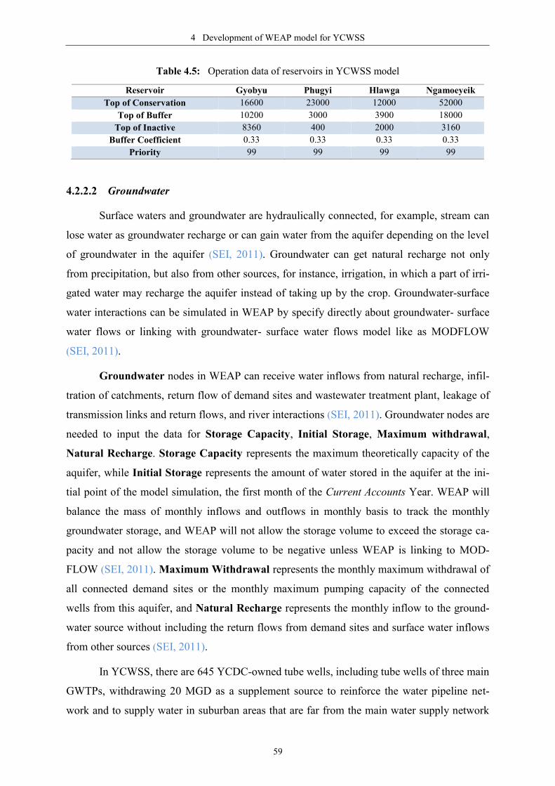
4 Development of WEAP model for YCWSS
59
Table 4.5: Operation data of reservoirs in YCWSS model
Reservoir Gyobyu Phugyi Hlawga Ngamoeyeik
Top of Conservation 16600 23000 12000 52000
Top of Buffer 10200 3000 3900 18000
Top of Inactive 8360 400 2000 3160
Buffer Coefficient 0.33 0.33 0.33 0.33
Priority 99 99 99 99
Groundwater 4.2.2.2
Surface waters and groundwater are hydraulically connected, for example, stream can
lose water as groundwater recharge or can gain water from the aquifer depending on the level
of groundwater in the aquifer (SEI, 2011). Groundwater can get natural recharge not only
from precipitation, but also from other sources, for instance, irrigation, in which a part of irri-
gated water may recharge the aquifer instead of taking up by the crop. Groundwater-surface
water interactions can be simulated in WEAP by specify directly about groundwater- surface
water flows or linking with groundwater- surface water flows model like as MODFLOW
(SEI, 2011).
Groundwater nodes in WEAP can receive water inflows from natural recharge, infil-
tration of catchments, return flow of demand sites and wastewater treatment plant, leakage of
transmission links and return flows, and river interactions (SEI, 2011). Groundwater nodes are
needed to input the data for Storage Capacity, Initial Storage, Maximum withdrawal,
Natural Recharge. Storage Capacity represents the maximum theoretically capacity of the
aquifer, while Initial Storage represents the amount of water stored in the aquifer at the ini-
tial point of the model simulation, the first month of the Current Accounts Year. WEAP will
balance the mass of monthly inflows and outflows in monthly basis to track the monthly
groundwater storage, and WEAP will not allow the storage volume to exceed the storage ca-
pacity and not allow the storage volume to be negative unless WEAP is linking to MOD-
FLOW (SEI, 2011). Maximum Withdrawal represents the monthly maximum withdrawal of
all connected demand sites or the monthly maximum pumping capacity of the connected
wells from this aquifer, and Natural Recharge represents the monthly inflow to the ground-
water source without including the return flows from demand sites and surface water inflows
from other sources (SEI, 2011).
In YCWSS, there are 645 YCDC-owned tube wells, including tube wells of three main
GWTPs, withdrawing 20 MGD as a supplement source to reinforce the water pipeline net-
work and to supply water in suburban areas that are far from the main water supply network

4 Development of WEAP model for YCWSS
60
of YCWSS. To study the groundwater system of Yangon City, there is no proper document
and reliable paper to get the data about it. Therefore, some reasonable data are assumed to
simulate the groundwater system. Storage Capacity for the aquifers is left blank by assuming
unlimited storage capacity, and Initial Storage of the aquifers are estimated by using FAO
groundwater potential data for lower Ayeyarwady delta region and the corresponding town-
ship areas where groundwater projects are located to represent the storage amount of the aqui-
fers at the beginning of simulation. Lower Ayeyarwady river basin, from the confluence with
Chindwin to its mouth, has about 95600 km2 of the catchment area and 153.249 km
3 of
groundwater potential (Ti & Facon, 2004). Monthly actual maximum withdrawal data only
from YCDC owned tube wells are used to represent Maximum Withdrawal data, and Natu-
ral Recharge data is calculated using estimated effective natural recharge rate 100 mm/year
and estimated effective area to recharge, i.e. 50 % of total area (JICA & YCDC, 2002; Döll &
Fiedler, 2007; Taylor, 2013). The data used in groundwater simulation of YCWSS are listed
in the following Table 4.6.
Table 4.6: Data of groundwater sources of YCWSS
Groundwater Source South Dagon
GWTP
Thaephyu
GWTP
Yangon Pauk
GWTP
YCDC Tube
Wells
Storage Capacity unlimited unlimited unlimited unlimited
Initial storage 59888 MG 23977 MG 24841 MG 82694 MG
(Total Area) 170.16 km2
68.13 km2
70.58 km2
234.96 km2
Monthly Maximum Withdrawal 60.84 MG 30.42 MG 30.42 MG 486.67 MG
Monthly Natural Recharge 155.98 MG 55.77 MG 58.82 MG 215.38 MG
Rivers 4.2.2.3
Rivers and diversions in WEAP represent river nodes (river reservoirs nodes, Run-of-
river hydropower nodes, flow requirement nodes, withdrawal nodes, diversion nodes, tribu-
tary nodes, return flow nodes, streamflow gauges) connected by river reaches, and other rivers
may flow in or out of a river (SEI, 2011). Head flow data of the river and the maximum in-
flow of the diversions are necessary to insert for the simulation of the rivers and diversions
system.
Even though Yangon City are surrounded by 6 rivers and 1 diversion, such as Yangon
River, Bago River, Hlaing River, Kokkowa River, Panhlaing River, Toe River, Ngamoeyeik
creek and Twantay Canal, there is no water supply from river source in YCWSS till now. In
the future plan of YCDC and JICA, these rivers are potential water sources for the expansion

4 Development of WEAP model for YCWSS
61
of YCWSS and two river water supply projects, Kokkowa river project and Toe river project,
are proposed to establish for future increased water demand. However, these projects are not
active in Current Accounts, so about the data of rivers and projects will be discussed in the
respective future scenarios.
Transmission links 4.2.2.4
Transmission links represent water transmission from reservoir, rivers, groundwater,
and other water supplies to satisfy the required demand at demand sites as well as the trans-
mission of wastewater outflows from demand sites and WWTPs to other demand sites for
reuse, and Supply preference for each transmission link need to define for the water alloca-
tion (SEI, 2011). WEAP allocates water according to the demand priority if one supply
source has more than one demand site and according to the supply preferences if a demand
site has connections with more than one supply source (SEI, 2011).
Linking Rules in WEAP specify the mix of supply from multiple sources to analyst
the observed allocation patterns in the Current Accounts and future scenarios of the model by
defining Maximum Flow (Volume) to restrict the supply from a source, Maximum Flow
(Percent of Demand) to restrict the flow using percent of the total requirement of demand
site (SEI, 2011). Loss from System, as a percent of flow passing through links, represents the
evaporation and leakage losses that will disappear from the system and Loss to Groundwater
refers to the leakage losses that flow into a groundwater node.
In this YCWSS model, there are 13 transmission links, which are connecting the sup-
ply source to only one demand site, Yangon City, via Yegu Ps and Ngamoeyeik WTP. The
maximum capacities of the sources are used as maximum flows of the transmission links in
this model, and there is no constraint in every link and the supply preferences for all nodes is
taken as 1 referring as first priority. Losses from the system in transmission links of surface
water sources are used as 66% to represent NRW amount of Yangon City, however, that of
groundwater sources are takes as 33% (half of NRW) because groundwater transmission pipe-
line system are shorter and leakage from this system is also smaller comparing with surface
water system. Losses from system of the link from Ngamoeyeik reservoir to Ngamoeyeik
WTP is assumed as 10% to represent the open channel transmission links and evaporation
losses from it. Losses to Groundwater of all links are assumed as zero. The detail input data
are summarised in the following Table 4.7.

4 Development of WEAP model for YCWSS
62
Table 4.7: Data of Transmission links in YCWSS
Transmission Links
From To
Maximum
Flow (Volume)
Maximum Flow
(% of demand)
Supply
Preference
Loss from
System
Loss to
Groundwater
Phugyi R Yegu PS 54 MGD No constraint 1 66 0
Hlawga R Yegu PS 14 MGD No constraint 1 66 0
Gyobyu R Yegu PS 27 MGD No constraint 1 66 0
Ngamoeyeik R WTP 45 MGD No constraint 1 10 0
Yegu PS Yangon City 95 MGD No constraint 1 - 0
Ngamoeyeik WTP Yangon City 45 MGD No constraint 1 66-10 0
South Dagon GWTP Yangon City 2 MGD No constraint 1 33 0
Thaephyu GWTP Yangon City 1 MGD No constraint 1 33 0
YCDC Tube Wells Yangon City 16 MGD No constraint 1 33
Yangon Pauk GWTP Yangon City 1 MGD No constraint 1 33 0
Lagunpyin R Yangon City Not active in Current Accounts
Kokkowa River Yangon City Not active in Current Accounts
Toe River Yangon City Not Active in Current Accounts
Runoff and infiltration 4.2.2.5
Runoff/infiltration links represent the runoff and infiltration from catchments to res-
ervoirs, rivers, and groundwater nodes and Runoff Fraction values for branches are needed to
define. In this model, five runoff links from five catchments are connected with their corre-
sponding reservoirs and runoff fraction values for all links are taken as 100%.
Return flow 4.2.2.6
Return flow links represent the flow of water, which is not consumed at a demand
site, to WWTPs, river or groundwater node, and other demand sites by defining as a percent-
age of outflows for Return Flow Routing, Loss from System, and Loss to Groundwater,
and Gain from Groundwater. About 90 % of water coming out from Yangon City is directly
re-entered to the environment and only 10% can be treated in WWTP, and after that, dis-
charged into Yangon River. To represent this situation of YCWSS, the listed input data in
Table 4.8 are used in this model.
Table 4.8: Data of Return Flows in YCWSS
Return Flow
From To
Return Flow
Routing (%)
Loss from
System (%)
Loss to
Groundwater (%)
Gain from
Groundwater (%)
Yangon City WWTP 10% 0 0 0
Yangon City Yangon River 90% 0 0 0
WWTP Yangon River 100% 0 0 0

4 Development of WEAP model for YCWSS
63
4.2.3 Others
Waste water treatment plant 4.2.3.1
Wastewater treatment plants in WEAP receive wastewater from demand sites, and
treat it to remove pollutants, and then return treated water to other demand sites, river or other
supply sources, and they are mainly used in water quality analysis. In YCWSS, there is only
one WWTP with 1 MGD treatment capacity and the consumption of water in this WWTP is
assumed as 16% of the inflow for this model simulation.
Key Assumption and Other Assumptions 4.2.3.2
In WEAP, Key Assumptions and Other Assumptions are used to create user-defined
variables for all major modeling assumptions, particularly those will vary from scenario to
scenario, to view and edit them conveniently (SEI, 2011). Key Assumptions are useful for
applying the same expression in multiple places in the model or highlighting the major model-
ling assumption, and less important intermediate variables are defined as Other Assumptions
(SEI, 2011). In this model, the annual population growth rate is defined as a key assumption
to change easily in different scenarios and to use easily in multiple places.
After the WEAP model of YCWSS had been developed, the reference scenario to rep-
resent the current situation of the system and other alternative scenarios to represent the
changes of system, such as socio-economic changes, climate changes, management changes
in both demand and supply sides, would be created for the simulation of future options in
YCWSS.

5 Creation of Scenarios in YCWSS-WEAP model
64
5 Creation of Scenarios in YCWSS-WEAP model
To implement the sustainable link between increasing water scarcity and growing wa-
ter demand is becoming a challenge for the future in water management field. To explore the
future option for water resources planning and management in the most sustainable way,
IWRM models that can see the impacts of future trends are required. These models simulates
to understand the processes and to analyse the future scenarios. In the model development, the
real processes must be clearly comprehended to mimic these in the model, however the most
relevant processes should be concentrated to simplify the model. Times-scale and spatial reso-
lution are the main components in sustainable water resources management. The most im-
portant aspect of applying models is to explore indirect impact external driven scenarios, such
as population growth and climate change, and direct impact management scenarios by water
managers and policy makers, such as changes in reservoir operations, water allocation and
agricultural/irrigation practices (See in Figure 5.1) (Immerzeel & Droogers, 2008).
Figure 5.1: The basic concept of scenario analysis in IWRM model (Immerzeel & Droogers, 2008)
Scenario analysis can answer the ‘what if’ questions in a water supply system, by
comparing the reference or business-as-usual scenario, which are developed by using the ac-
tual data for the understanding of current trend, and other scenarios, which are built on this
reference scenario with changes on both demand and supply sides (SEI, 2011). This section
will describe different scenarios based on the feasible changes in YCWSS to advance in
WEAP model for city water supply options extending the current situation of the Current Ac-
counts Year (2013) to the future until the Last Year of Scenarios (2040) with monthly time
Models
Remote Sensing
Observations
Analysis
Statistics
Past
Today
Future Options for future
- Technical
- Socio-economic
- Policy oriented
Understand past water resources
Understand current water resources
?
Trend

5 Creation of Scenarios in YCWSS-WEAP model
65
steps. The scenario analysis in WEAP will give out the results for flexible representation of
the consequences of alternative development patterns and supply dynamics.
In this study, different scenarios relating with the external changes and different man-
agement alternatives will be created for the analysis of future water supply options in
YCWSS. At first, reference scenario will be built to represent the current situation of the sys-
tem. Then, the other scenarios, which represent the possible changes in the system supply
sources and demand sites, will be constructed to study the impacts of these changes by com-
paring with the reference scenario.
5.1 Reference Scenario
Reference scenario, also known as a default scenario or business-as-usual scenario,
is established from the Current Accounts, which represents the basic definition of the current
system including the specification of supply and demand data for the first year of the study on
a monthly basis, to stimulate likely evolution of the system without intervention (SEI, 2011).
Reference scenario carries forward the current data into the entire time horizon in which no
major changes are imposed and serves as a point of comparison for the other scenarios in
which changes are made in the system data.
In this study, Reference Scenario will be applied to analyse the situation of YCWSS
without any development in of the system except the population growth with normal growth
rate 2.5%, Second phase of Ngamoeyeik WTP, and Lagunpyin reservoir water supply project,
which is ongoing project started in 2013 and will finish in 2015. Design supply capacity of
Lagunpyin reservoir is 40 MGD, and it will be initiated its operation in 2015. To set up this
Reference Scenario (2014-2040), the additional data for population growth, new water
sources are needed to add in it. Concerning about the population growth, the normal growth
rate 2.5% is used to project the population until the end of study period. The second phase of
Ngamoeyeik WTP was initiated in 2014, and the water supply capacity was increased from 45
MGD to 90 MGD. So, to represent these changes in the model, the maximum flow volume in
the transmission link from Ngamoeyeik Reservoir to Ngamoeyeik WTP and that from Nga-
moeyeik WTP to Yangon City are raised from 45 MGD to 90 MGD. Then, ongoing project
using water source from Lagunpyin Reservoir and its water source, Lagunpyin Catchment,
and its transmission links with source and demand site are added in this scenario by using the
data, which are described in Table 5.1, and the climate data for this catchment and reservoir is
used the data of the nearest meteorological station, Hmawbi station.
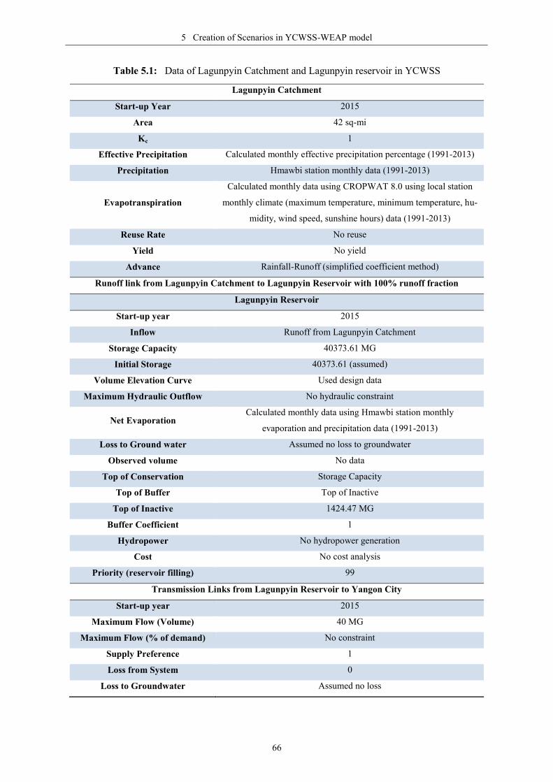
5 Creation of Scenarios in YCWSS-WEAP model
66
Table 5.1: Data of Lagunpyin Catchment and Lagunpyin reservoir in YCWSS
Lagunpyin Catchment
Start-up Year 2015
Area 42 sq-mi
Kc 1
Effective Precipitation Calculated monthly effective precipitation percentage (1991-2013)
Precipitation Hmawbi station monthly data (1991-2013)
Evapotranspiration
Calculated monthly data using CROPWAT 8.0 using local station
monthly climate (maximum temperature, minimum temperature, hu-
midity, wind speed, sunshine hours) data (1991-2013)
Reuse Rate No reuse
Yield No yield
Advance Rainfall-Runoff (simplified coefficient method)
Runoff link from Lagunpyin Catchment to Lagunpyin Reservoir with 100% runoff fraction
Lagunpyin Reservoir
Start-up year 2015
Inflow Runoff from Lagunpyin Catchment
Storage Capacity 40373.61 MG
Initial Storage 40373.61 (assumed)
Volume Elevation Curve Used design data
Maximum Hydraulic Outflow No hydraulic constraint
Net Evaporation Calculated monthly data using Hmawbi station monthly
evaporation and precipitation data (1991-2013)
Loss to Ground water Assumed no loss to groundwater
Observed volume No data
Top of Conservation Storage Capacity
Top of Buffer Top of Inactive
Top of Inactive 1424.47 MG
Buffer Coefficient 1
Hydropower No hydropower generation
Cost No cost analysis
Priority (reservoir filling) 99
Transmission Links from Lagunpyin Reservoir to Yangon City
Start-up year 2015
Maximum Flow (Volume) 40 MG
Maximum Flow (% of demand) No constraint
Supply Preference 1
Loss from System 0
Loss to Groundwater Assumed no loss

5 Creation of Scenarios in YCWSS-WEAP model
67
5.2 Other Scenarios
Besides the reference scenario, other scenarios are developed to understand the im-
pacts of external changes in YCWSS and the effects of management practises in both demand
and supply sides in this system. The following future scenarios will be developed and ana-
lysed in this study.
External driven scenarios
Socioeconomic change scenarios
High Population Growth (HPG) scenario: It analyses the situation with high popula-
tion growth rate 3.5%.
Low Population Growth (LPG) scenario: It analyses the situation with low popula-
tion growth rate 1.5%.
Higher Living Standards (HSL) scenario: It analyses the situation of increase in wa-
ter consumption rate from the present rate 30 gpcd to 40 gpcd in 2040 because of
higher living standards.
Climate change scenario
Climate Change (CC) scenario: It analyses the situation of water supply system under
climate change data.
Management scenarios
Demand-side management (DSM) scenarios
DSM-Water-Pricing Policy (WPP) scenario: It analyses the situation with changing
water-pricing policy.
DSM-Sustainable Water Source (SWS) scenario: It analyses the situation with intro-
ducing new sustainable water sources in demand-side such as rainwater harvesting.
Supply-side management (SSM) scenarios
SSM-NRW Control (NRWC) scenario: It analyses the situation with NRW control
management plan.
SSM-Alternative Supply Source (ASS) scenario: It analyses the situation with the de-
velopment of the system start-using alternative water source, river water source, and
stop-using groundwater source in 2025.

5 Creation of Scenarios in YCWSS-WEAP model
68
Based on these future scenarios, the best management option for future water supply
of Yangon City in the worst condition will be figured out by integrating these different sce-
narios, as the following Figure 5.2, in the scenario analysis of YCWSS-WEAP model.
Figure 5.2: Different options for future water supply in Yangon City
5.2.1 External driven scenarios
Socioeconomic Change Scenarios 5.2.1.1
Yangon City is the largest urbanization area in the country because of being the former
capital of the country. According to the report of Urban Planning Department of YCDC, the
percentage of urban population in Yangon Region in 2012 is 76%, whereas the urban popula-
tion percentage in the country is only 30% (Aung, 2013). Moreover, Yangon region contrib-
utes around 22% to the total national GDP as well as the region has the highest per capita
GDP in the Union of Myanmar (Aung, 2013). According to the data from Urban and Regional
Planning Division of Ministry of construction, Special Economic Zone, National Government
Project, is start implementing in Yangon Region, and its first phase will start operate in 2015
with labour force around 50,000 and it will be developed gradually to the final state with the
labour force about 200,000 in 2035. This means that migration of people from rural areas will
be increased because of increasing job opportunities together with urbanization and industrial-
ization.
Nowadays, Yangon City is encountering the socioeconomic changes, however, there is
no reliable data about population because there was no national census data in Myanmar since
1981 until the end of 2013. In April 2014, Myanmar Government was taken the national soci-
oeconomic data all over the country in order to use the national level development project by
External Driven Scenarios Management Scenarios
High
Population
Growth Rate
Normal
Population
Growth Rate
Low
Population
Growth Rate
Climate
Change
Higher
Living
Standards
Demand-side management
Sustainable Water Source
Demand-side management
Water Pricing Policy
Supply-side management
Alternative Supply Source
Supply-side management
NRW -Control

5 Creation of Scenarios in YCWSS-WEAP model
69
using these data. To draw the city’s master plan and urban development projects, Urban Plan-
ning Department of YCDC is forecasted that the city’s population will become 10 million in
2040, by using the past population growth rate in the period 1993-2013 that is 2.5 %. In addi-
tion, another high population growth scenario is also predicted by using 3.5 % because of na-
tional development projects in the city region, urbanization, and industrialization, and migra-
tion of rural people. On the other hand, the global forecasted data for the population and
population growth rate of Yangon City is lower than the local data, and the fertile rate is de-
clining especially in urban region together with increasing number of single and unmarried
person. Therefore, the scenario with low population growth rate also should be considered to
forecast the future population of Yangon City. The forecasted data using different population
growth rate are illustrated in the following Figure 5.3.
Figure 5.3: Forecasted data for future population growth rate
Since population growth is the main threatening reason for the water crisis, water
planner wants to see how different population growth will affect on water sustainability (Ke,
2009; Ke & Qin, 2011 May). In this study, the scenarios related with population change will
simulate using high population growth rate 3.5 % and low population growth rate 1.5 % and
then the results of these scenarios will be analysed by comparing with the reference scenario,
which is using normal population growth rate 2.5 %, to know the impact of this changes. The
following two scenarios, only difference between these scenarios and the Reference Scenarios
is the population growth rate, will be developed to explore the sensitivity to population.
0
2
4
6
8
10
12
14
1963 1973 1983 1993 2003 2013 2023 2033
Pop
ula
tion
(m
illi
on
)
Year
Forecasted Population trends of Yangon City
With Normal Growth Rate 2.5%
With High PGR 3.5%
With Low PGR 1.5%

5 Creation of Scenarios in YCWSS-WEAP model
70
High Population Growth (HPG) Scenario: This scenario looks at the impact of increasing
population growth rate for Yangon City from normal population growth rate 2.5 % to 3.5 be-
cause of urbanization, industrialization, and migration of people from rural areas. Under this
scenario, the Annual Population Growth Rate in Key Assumption is input as 3.5 % and the
Annual Activity Level of Yangon City is calculated using this input data.
Low Population Growth (LPG) Scenario: This scenario looks at the impact of decreasing the
population growth rate for Yangon City from normal population growth rate 2.5 to 1.5 be-
cause of the declination of the fertile rate. For WEAP analysis under this scenario, the Annual
Population Growth Rate in Key Assumption is changed as 1.5 %, and the Annual Activity Lev-
el of Yangon City is projected applying this low rate.
Parallel with urbanization and economic development in Yangon City, water con-
sumption rate will increase in order to achieve the higher living standards. Water consumption
rate is becoming significantly increased due to rapid economic development, urbanization,
migration, lifestyle changes and other social transitions in Asia Countries (Hubacek et al.,
2009). According to the results of JICA research, the more urbanized city has the better water
supply service and the water consumption rate for each person in that city is higher than the
other cities (JICA & YCDC, 2014). The performance indicators (PIs), which can determine
the service level of the city water supply system, of Southeast Asia cities are listed in Table
5.2, and the most urbanized city, Singapore, has the better water supply service with 100%
coverage, 4% NRW, and 58 gpcd consumption rate.
Table 5.2: Performance Indicators of water supply service in cities of Southeast Asia countries
(JICA & YCDC, 2014)
Country Indonesia Thailand Vietnam Singapore Philippine Cambodia Malaysia Lao PDR
City Jog Jakata Bangkok Ho-Chi-Minh Singapore Davao Phonon
Penh
Kuala
Lumpur Vientiane
Population
(million) 8.7 7.958 5.976 4.737 4.468 1.519 1.493 0.799
Water
Coverage (%) 62 93 84 100 59 80 100 50
Water Use Rate
(gpcd) 25 37 32 58 36 38 83 65
NRW (%) 50 29 41 4 25 6 35 28
Water Price
(€ per m3) 0.53 0.34 0.2 0.71 0.26 0.21 0.34 0.09
Statistical Year 2007 2009 2009 2008 2009 2007 2007 2007

5 Creation of Scenarios in YCWSS-WEAP model
71
For the improvement of water supply service in Yangon City as other Asian cities,
YCDC put a plan to serve higher water consumption amount year-by-year becoming higher
living standard with economic development in the future. In this study, the situation related
with increased water consumption rate will analyse using the future target value of YCDC-
JICA Master Plan, that is to improve the water supply for increased consumption rate from
the present value 30 gpcd to 35 gpcd in 2025 and 40 gpcd in 2040.
Higher Living Standard (HSL) Scenario: This scenario looks at the impact of increasing
water consumption rate corresponding to the higher living standard because of the economic
development of Yangon City. For this scenario, the Water Use Rate for Yangon City is
changed by using the smooth inclination form 10950 imperial gallons per person, i.e. 30 gpcd
is multiplied by 365 days, in 2013 to 12775 imperial gallons per person in 2025 and 14600
imperial gallons per person in 2040 by using 30 gpcd and 40 gpcd rates.
Climate change Scenario 5.2.1.2
Climate change is important for the water supply system because it can change the ex-
isting water management situations and increase the requirement for new management op-
tions (Mounir et al., 2011). Climate change is important to water planners and decision mak-
ers but climate change can make confound water resources planning because of its uncertain
effects and difficult prediction (Conway et al., 2009; Mounir et al, 2011). For the analysis of
climate change effect in YCWSS, Climate Change (CC) scenario is constructed by using the
climate data acquired from climate change model.
Climate Change (CC) Scenario: This scenario looks at the impact of climate change in Yan-
gon City using the downloaded Global Climate Model data set of the Coupled Model Inter-
comparison Project, Phase 5 (GCM: CMIP5 full set) from KNMI (Koninklijk Netherlands
Meteorological Institute) Climate Explorer website. GCM: CMIP5 (full set) includes multiple
realisations of each model, downweighed to be the same weight for each model and there are
four representative concentration pathways (RCPs), such as RCP2.6, RCP4.5, RCP6.0, and
RCP8.5. In this study for YCWSS, RCP6.0, a stabilization scenario in which greenhouse gas
emissions rise quickly up to 2060 and then decrease, is used to get the climate data set of
Hmawbi weather station located at 17.16 ºN and 96.06 ºE in Yangon Region for the period
2014-2040. Under this scenario, the future climate data (2014-2040) of the catchments, such
as precipitation and evapotranspiration, are applied by GCM model data, instead of cycling
the historical data as in the reference scenario.
5 Creation of Scenarios in YCWSS-WEAP model
72
5.2.2 Management Scenarios
As urban water, utilities are facing increasingly water scarcity problems due to popula-
tion growth, climate change and environmental issues, city water planners are trying to find
management strategies not only to advance the water supply but also to reduce the water de-
mand (Baerenklau, Schwabe & Dinar, 2013). To solve the encountering problems of YCWSS,
and the indirect effects of external changes, local authorities and water managers of Yangon
City also need to find out the strategies for both demand and supply sides management op-
tions. In this study, two demand-side scenarios and two supply side scenarios will be generat-
ed and analysed to help the decision makers for alternative policy, management options, and
future development plans.
Demand-side Management (DSM) Scenarios 5.2.2.1
Water-pricing policies, water-saving technologies, and public awareness are some im-
portant management strategies to control the demand-side. In general, water authorities prac-
tise two kinds of water-pricing system, flat-rate system and block-rate system or also known
as tiered water-pricing system. Tiered water-pricing system charge with a higher price per
unit water for higher consumption rates, thus it encourages users to reduce their water con-
sumption. Using tiered water-pricing system in residential areas can reduce at least 18 percent
of the total water demand, although the reduction is achieved gradually (Baerenklau, Schwabe
& Dinar, 2013). In addition, the amount of water consumption can drop 5 % when the water
price is increasing about 10%, and that can drop 10 % when the water price is increasing
about 40 % (Guo et al., 2006). Increasing water price can save the domestic water demand,
and the water demand saving amount abstained by increasing water price in tiered water-
pricing system is more effective than that in flat-rate system (Baerenklau, Schwabe & Dinar,
2013). The benefits generated by this pricing strategies such as water price change and water-
pricing system change could be simulated in WEAP model estimating the demand reduction
amount, such as annual activity level, annual water use rate, and DSM saving percent etc.
With the aggregated approach for DSM, the estimated reduction fraction of total demand for a
demand site due to DSM programs must enter under DSM Savings (SEI, 2011). In YCWSS,
flat rate is practising for water-pricing system with unit water-price about 0.07 €/m3 that is
much lower than other Asian countries (see in Table 5.2). Therefore, YCDC is drawing a plan
about the water pricing policy by increasing the unit price and changing to the tiered system.
To study for the effects of this plan in YCWSS, the first DSM scenario by water-pricing poli-
cy is constructed using assumed water saving amount with 20%.

5 Creation of Scenarios in YCWSS-WEAP model
73
Moreover, sustainable water sources, such as rainwater, seawater and recycle-water,
and water-saving technologies should be introduced to the city dwellers to improve the public
awareness and to reduce the water demand from the urban area. However, desalination and
recycling technologies are not suited with the developing countries because of high cost and
energy requirements, and rainwater harvesting (RWH) is a potential technology for Yangon
City. Using RWH in urban areas could solve not only the current water shortage problems but
also the urban stream degradation and flooding problems (Fletcher et al., 2008). The quantity
of harvested rainwater amount of RWH in urban areas can be simply calculated by multiply-
ing RW harvested area with rainfall by using system efficiency 80% (UNEP, 2009). In Yan-
gon City, even though it is impossible to implement the RWH technique in existing buildings,
new constructions are possible to install the RWH facilities. Therefore, local authorities
should encourage practising this technique in new buildings not only for demand control but
also for city flood control option. In this study, the second DSM scenario using sustainable
water source in demand side is built assuming one squared metre RW harvested area and one
cubic metre RW harvested storage amount for each increased person after the Current Ac-
counts year, and using system efficiency 80 %.
1st DSM - Water-Pricing Policy (WPP) Scenario: This scenario will point out the benefits of
water pricing policy by analysing a situation with DSM program that is changing from fixed
water-pricing policy to tiered water-pricing policy together with the increasing the water price
from current price amount to an affordability to pay amount from customer survey’s result.
Under this scenario, the DSM saving amount is assumed that 20 % could reduce in the total
monthly demand due to this change of water-pricing policy.
2nd
DSM - Sustainable Water Source (SWS) Scenario: This scenario will show the effects of
introducing sustainable water source in demand sites, in here Rainwater Harvesting (RWH) in
Yangon city. In YCWSS model, firstly, RWH supply is created and connected to the Yangon
City with transmission links via RWH reservoirs. This virtual RWH supply source and RWH
reservoir represent the RWH facilities of the newly constructed buildings in Yangon City af-
ter 2013. Precipitation data of Yangon City, harvested area, calculated by multiplying 1 m2
per capita rate with increased population in Yangon City after 2013 and 80 % efficiency rate,
are used for the data of RWH supply source. After that, this water supply source is linked
with RWH reservoir that represents the RW storage tanks in these building by assuming 1 m3
volume amount for each person, and then this reservoir is linked with Yangon City using sup-
ply preference as 2 representing second priority source for Yangon City.

5 Creation of Scenarios in YCWSS-WEAP model
74
Supply-side Management (SSM) scenarios 5.2.2.2
Extension of the system using the reliable water resources is one of the major solutions
to improve the water supply service, but controlling the physical water losses and commercial
losses in the system also can increase the water supply amount without disturbing the envi-
ronment and with less investment. Comparing with the other Asian countries, NRW amount
in Yangon City, i.e. 66%, is much higher, and EDWS should be responsible to reduce that
amount by laying a project and target plan to improve the quality and quantity of supply wa-
ter. Future target for NRW control in YCDC-JICA master plan is to reduce NRW amount
from 66% current amount to 15% in 2040 by using different improvement plans for the dif-
ferent non-revenue water sources. In this study, the first SSM scenario will construct concern-
ing about the NRW control project using these future target values for NRW that are men-
tioned in YCDC-JICA master plan.
Additionally, alternative water sources should develop to cover the water supply
amount for future water demand. The total water demand amount of Yangon City in 2040 will
be 400 MGD using 40 gpcd rate for 10 million people without including any losses from the
whole system. On the other hand, the total water supply amount in Yangon City is only 225
MGD including Ngamoeyeik WTP 2nd
Phase (45 MGD capacity) and Lagunpyin Reservoir
(40 MGD capacity) without including groundwater source. Therefore, EDWS proposed two
new water supply projects by using river water source from Kokkowa River and Toe River
(see in Table 3.11) and to stop using groundwater source in YCWSS in 2025 because of
groundwater table lowering, saline water intrusion, and land subsidence problems. The devel-
opment of the potential water source is necessary to meet the future water demand of Yangon
City, and Kokkowa River, which has minimum river discharge about 1045 m3/s, and Toe
River, which has about 2448 m3/s, are considered as potential water sources for Yangon City
according to the feasibility survey for these rivers. The survey data for this river by JICA and
MoAI are listed in the Table 5.3, and JICA study team calculated and estimated these data
using the flow rates and cross sections of the rivers that are measured by MoAI. These MoAI
report for river flow survey will be described in appendix B. As these river flows are much
greater than the required water demand of YCWSS in 2040, YCDC and JICA decided to use
these water as source and at present detail survey for the project are still processing. In draft
plan, YCWSS will use 240 MGD amount from Kokkowa River and 180 MGD from Toe Riv-
er by implementing phase by phase. These projects will construct as the second SSM scenario
by using alternative water sources to see the role of these projects in future water supply.

5 Creation of Scenarios in YCWSS-WEAP model
75
Table 5.3: Survey data for river water source (JICA & YCDC, 2014)
River
( capacity)
Minimum River
Discharge
Irrigation
Use
Maintenance
Use
Potential
Water Source
Project Target
Kokkowa
(240 MGD)
1045 m3/s 12 m
3/s 525 m
3/s 520 m
3/s
(9984MGD)
15 MGD (2020)
+ 45 MGD (2025)
+ 60 MGD (2030)
+ 120 MGD (2040)
Toe
(180 MGD)
2448 m3/s 0 m
3/s 1228 m
3/s 1220 m
3/s
(23424MGD)
15 MGD (2025)
+ 15 MGD (2030)
+ 30 MGD (2035)
+ 120 MGD (2040)
1st SSM - NRW Control (NRWC) scenario : This scenario will analyse a situation with estab-
lishment of NRW control management plan in YCWSS to decrease the NRW amount from
66% to 35% in 2025 and 15% in 2040 (same amount as future target of YCDC-JICA Master
Plan). In YCWSS-WEAP model, these data is input reducing the losses of transmission links,
as 66% NRW amount was used as transmission losses in the Current Accounts.
2nd
SSM - Alternative Supply Source (ASS) scenario: This scenario will inspect the situation
with development of the system using alternative source, river water from Toe River and
Kokkowa River, including stop-using groundwater source in 2025. Two new river water
source project will be added supposing minimum river flows (maintenance flow and irriga-
tion flow are already deducted ) as river flow for the whole year due to the lack of time series
data, however this assumption can use safely because these minimum flows are much higher
than the withdraw amounts by these projects. The supply preference values of the transmis-
sion links from these new sources to the city are taken as 2 whereas those values for the cur-
rent sources were used as 1. This means that Yangon City will prefer the old water sources to
check the role of the new water sources in YCWSS, and Yangon City will not use water from
new sources if there is no unmet demand in the system.
To be concluded, four external driven scenarios (such as HPG, LPG, HLS, and CC)
and four management scenarios (such as WPP, SWS, NRWC, and ASS) are generated in this
YCWSS-WEAP model to comprehend the impacts of these effects in future water supply-
demand system of Yangon City by comparing with the reference scenario and to assist the
planners to choose the best management option for the future YCWSS.

6 Simulation and Evaluation of Scenarios
76
6 Simulation and Evaluation of Scenarios
This part will present initially about the current situation of YCWSS by evaluating the
simulated results of the Reference Scenario to understand the current situation of YCWSS,
and these Reference Scenario results will also be used to verify this YCWSS-WEAP model is
fit to represent the actual situation of YCWSS. After that, the positive and negative impacts of
the different scenarios will be evaluated by comparing and contrasting the results of the Ref-
erence Scenario and the other eight scenarios, which represent possible alternatives of
YCWSS in the future and the reliability of YCWSS in different scenarios, will be also pointed
out in those cases.
Water flows through the system in WEAP is guided by the principle of mass balance
like other simulation models. After entering the data for study area, WEAP can run its month-
ly simulation and report the results of projections for all aspects of the system, concerning
about demand sites, supply sources, water quality, and financial data (SEI, 2011). One of the
strengths of WEAP model is that results can be presented in graphs, tables, or maps. In addi-
tion, the results can be exported directly to Microsoft Excel for further data analysis, and there
are multiple options to aggregate the results in time, space or different components to com-
pare different scenarios easily (Van Loon & Droogers, 2006). The most important data for the
future management of YCWSS will be presented in this section, mainly focusing on the re-
sults for demand coverage and unmet demand of Yangon City in the Reference Scenario (the
Current Accounts) and the impacts of other alternative scenarios on demand coverage.
6.1 Evaluation of the Current YCWSS in Reference Scenario
The present situation of YCWSS can be evaluated according to the result of the Cur-
rent Accounts, Reference Scenario. Before simulation of the scenarios, it is necessary to do
the calibration and validation in WEAP, but WEAP has no automatic calibration operation
and the changes implemented were tested manually by comparing the simulated and observed
time series (SEI, 2011). In WEAP models, flows data are mostly used for calibration of the
models. On the other hand, Water supply-demand models are complicated because they are
required not only to simulate human behaviour for changes in demand but also to simulate
physical processes of the water sources and facilities. This means that model calibration and
validation is extremely difficult and has often been neglected in the past (McCartney & Ar-

6 Simulation and Evaluation of Scenarios
77
ranz, 2007). In this YCWSS model, the calibration and validation of the model could not do
properly because of the insufficient data and the method used for rainfall-runoff (simplified
coefficient) method simulation. Nevertheless, the model performance was checked by using
observed volume data of reservoirs of YCWSS from 2005 to 2013, and water coverage data
of Yangon City in 2013. The Figure 6.1 shows that the graphs of the simulated data and the
observed data for the reservoirs of YCWSS for the period from 2005 to 2013.
(a) (b)
(c) (d)
Figure 6.1: Observed volumes and simulated volumes of (a) Gyobyu Reservoir (b) Hlawga Reser-
voir (c) Phugyi Reservoir (d) Ngamoeyeik Reservoir (2005-2013)
According to these graphs, the trends of the curves are the same for the whole time se-
ries but the simulated volume curves are higher and earlier than the observed data. This
YCWSS model is simulated by using the rainfall-runoff (simplified coefficient) method with
land use data (area of the catchment, crop coefficient (Kc), effective precipitation) and climate
data (precipitation, reference evapotranspiration data), and only Kc value can be used to cali-
brate the model. However, according to the sensitivity analysis results, that Kc value is not a
sensitive parameter to calibrate this model. Mugatsia (2010) also pointed out that soil mois-
Observed Volume Storage Volume
Observed and Simulated Reservoir VolumeReservoir: Gyobyu Reservoir, Scenario: Reference Scenario
Jan
20
05
Ap
r 2
00
5
Au
g 2
00
5
Dec
20
05
Ap
r 2
00
6
Au
g 2
00
6
Dec
20
06
Ap
r 2
00
7
Au
g 2
00
7
Dec
20
07
Ap
r 2
00
8
Au
g 2
00
8
Dec
20
08
Ap
r 2
00
9
Au
g 2
00
9
Dec
20
09
Ap
r 2
01
0
Au
g 2
01
0
Dec
20
10
Ap
r 2
01
1
Au
g 2
01
1
Dec
20
11
Ap
r 2
01
2
Au
g 2
01
2
Dec
20
12
Ap
r 2
01
3
Au
g 2
01
3
Dec
20
13
Bil
lio
n I
mp
. G
allo
n
16.5
16.0
15.5
15.0
14.5
14.0
13.5
13.0
12.5
12.0
11.5
11.0
10.5
10.0
9.5
9.0
Observed Volume Storage Volume
Observed and Simulated Reservoir VolumeReservoir: Hlawga Reservoir, Scenario: Reference Scenario
Jan
20
05
Ap
r 2
00
5
Au
g 2
00
5
Dec
20
05
Ap
r 2
00
6
Au
g 2
00
6
Dec
20
06
Ap
r 2
00
7
Au
g 2
00
7
Dec
20
07
Ap
r 2
00
8
Au
g 2
00
8
Dec
20
08
Ap
r 2
00
9
Au
g 2
00
9
Dec
20
09
Ap
r 2
01
0
Au
g 2
01
0
Dec
20
10
Ap
r 2
01
1
Au
g 2
01
1
Dec
20
11
Ap
r 2
01
2
Au
g 2
01
2
Dec
20
12
Ap
r 2
01
3
Au
g 2
01
3
Dec
20
13
Bil
lio
n I
mp
. G
allo
n
12.0
11.0
10.0
9.0
8.0
7.0
6.0
5.0
4.0
3.0
Observed Volume Storage Volume
Observed and Simulated Reservoir VolumeReservoir: Phugyi Reservoir, Scenario: Reference Scenario
Jan
20
05
Ap
r 2
00
5
Au
g 2
00
5
Dec
20
05
Ap
r 2
00
6
Au
g 2
00
6
Dec
20
06
Ap
r 2
00
7
Au
g 2
00
7
Dec
20
07
Ap
r 2
00
8
Au
g 2
00
8
Dec
20
08
Ap
r 2
00
9
Au
g 2
00
9
Dec
20
09
Ap
r 2
01
0
Au
g 2
01
0
Dec
20
10
Ap
r 2
01
1
Au
g 2
01
1
Dec
20
11
Ap
r 2
01
2
Au
g 2
01
2
Dec
20
12
Ap
r 2
01
3
Au
g 2
01
3
Dec
20
13
Bil
lio
n I
mp
. G
allo
n
23.0
22.0
21.0
20.0
19.0
18.0
17.0
16.0
15.0
14.0
13.0
12.0
11.0
10.0
9.0
8.0
Observed Volume Storage Volume
Observed and Simulated Reservoir VolumeReservoir: Ngamoeyeik Reservoir, Scenario: Reference Scenario
Jan
20
05
Ap
r 2
00
5
Au
g 2
00
5
Dec
20
05
Ap
r 2
00
6
Au
g 2
00
6
Dec
20
06
Ap
r 2
00
7
Au
g 2
00
7
Dec
20
07
Ap
r 2
00
8
Au
g 2
00
8
Dec
20
08
Ap
r 2
00
9
Au
g 2
00
9
Dec
20
09
Ap
r 2
01
0
Au
g 2
01
0
Dec
20
10
Ap
r 2
01
1
Au
g 2
01
1
Dec
20
11
Ap
r 2
01
2
Au
g 2
01
2
Dec
20
12
Ap
r 2
01
3
Au
g 2
01
3
Dec
20
13
Bil
lio
n I
mp
. G
allo
n
52
50
48
46
44
42
40
38
36
34
32
30
28
26
24
22
Observed volume Simulated volume

6 Simulation and Evaluation of Scenarios
78
ture method with more detailed data should be used to model the hydrology of the catchment
with the aim of reducing the high peak hydrographs. It is obvious that there is some weakness
in this simplified coefficient method, which is a lack of consideration about interflow and
base flow processes and time of runoff concentration from the catchment to the reservoirs.
Hence, the simulated water volumes in reservoirs are higher than the actual observed vol-
umes, especially in the drought years as 2005 and 2010, and the simulated runoff are a bit
earlier than the observed data. In hydrology studies used for management purposes, total vol-
ume errors below 10% are very good, between 10% and 20% is good, and between 20% and
30% is fair (Ingol-Blanco & McKinney, 2009). In this study, the differences between 9-year
observed volume and model simulated volume in Gyobyu, Hlawga, Phugyi and Ngamoeyeik
reservoirs are -18%, -53 %, -9%, and -12% respectively, and the coefficient of determination
(R2) for these reservoirs are 0.17, 0.18, 0.31 and 0.35. This means that the model is over-
predicted and good to use for study according to the results of total volume errors, and ac-
cording to the results of R2, this model has high error variance.
Besides these supply-side results, the demand-side results also can be applied in the
model performance analysis. The result data for demand coverage amount and supply deliv-
ered amount in Yangon City are shown in the Figure 6.2, the average demand coverage in
Yangon City is about 31.16 % in 2013, and the average daily supply delivered amount in
Yangon City is about 47.94 MGD in 2013. These data are nearly the same (less than 5% devi-
ation) with the observed data, calculated depending on the actual data of EDWS (YCDC) in
2013, which is about 32.4 % for demand coverage and 50 MGD for daily supply amount in
Yangon City.
In WEAP, the water supply amount in transmission links from reservoirs to demand
site is controlled by using buffer coefficient only if the reservoir volume is lower than the
buffer zone. In this study, reservoirs of YCWSS are rarely encountered about that problem in
the past (2005-2013) not only in the simulated result but also in the actual observed data,
apart from some cases that Gyobyu and Hlawga reservoirs faced that problem in drought
years, 2005 and 2010 (see in Figure 6.1). Therefore, the observed and simulated water supply
amount in the transmission links is the same in this YCWSS model, and the weak point of
using rainfall-runoff (simplified coefficient) method for catchment simulation cannot disturb
the water supply system of Yangon City as long as the reservoirs level are lower than their
buffer zone. Therefore, this YCWSS model can be acceptable to use in the study for man-
agement purposes to analyse the future scenarios of water supply coverage in Yangon City.

6 Simulation and Evaluation of Scenarios
79
(a) (b)
Figure 6.2: (a) Demand coverage (b) Supply delivered amount in Yangon City (2013)
6.1.1 Estimation of Future Demand in YCWSS
According to the simulation results of Reference Scenario for water demand in Yan-
gon City, which are shown in Figure 6.3, the future water demand in Yangon City is expected
an increase from 4774 MG per month (154 MGD) in 2013 to 9300 MG per month (300
MGD) in 2040. According to the monthly average water-demand results, water demand in
Yangon City is forecasted that it will be high in the summer, especially in April, and relative-
ly low in other two seasons, the rainy season, and the cool season.
In this study, monthly water-consumption variation data was derived from the water-
meter bill income of EDWS and the problem is that the monthly water consumption amount
cannot get actual amount in March, which is the last month of the budget year. Staffs of
EDWS collect the water meter readings in third week of the month in March and in last week
of the month in the other months, thus, the water demand in March is the lowest comparing
with the other months. Moreover, Yangon City get high rainfall in the rainy season but the
water demand for this season is not much lower than other seasons, and it can be pointed out
that people in Yangon City mainly consume the piped water without using rainwater.
(a) (b)
Figure 6.3: Future demand of Yangon City in Reference scenario (a) 2013-2040 (b) monthly average
Yangon City Demand Site Coverage (%) in Yangon City
Scenario: Reference Scenario
Jan
20
13
Feb
20
13
Mar
20
13
Ap
r 2
01
3
May
20
13
Jun
20
13
Jul
20
13
Au
g 2
01
3
Sep
20
13
Oct
20
13
No
v 2
01
3
Dec
20
13
Per
cen
t
38.0
36.0
34.0
32.0
30.0
28.0
Yangon City Supply Delivered
Scenario: Reference Scenario
Jan
20
13
Feb
20
13
Mar
20
13
Ap
r 2
01
3
May
20
13
Jun
20
13
Jul
20
13
Au
g 2
01
3
Sep
20
13
Oct
20
13
No
v 2
01
3
Dec
20
13
Mil
lio
n I
mp
. G
allo
n
1,800
1,700
1,600
1,500
1,400
1,300
Yangon City Water Demand (not including loss, reuse and DSM)
Scenario: Reference Scenario
Jan
20
13
Jul
20
14
Jun
20
16
May
20
18
Ap
r 2
02
0
Mar
20
22
Feb
20
24
Jan
20
26
Dec
20
27
No
v 2
02
9
Oct
20
31
Sep
20
33
Au
g 2
03
5
Jul
20
37
Jun
20
39
Mil
lio
n I
mp
. G
allo
n
9,500
9,000
8,500
8,000
7,500
7,000
6,500
6,000
5,500
5,000
4,500
Yangon City Water Demand (not including loss, reuse and DSM)
Scenario: Reference Scenario, Monthly Average
Jan
uar
y
Feb
ruar
y
Mar
ch
Ap
ril
May
Jun
e
July
Au
gu
st
Sep
tem
ber
Oct
ob
er
No
vem
ber
Dec
emb
er
Mil
lio
n I
mp
. G
allo
n
6,900
6,800
6,700
6,600
6,500
6,400
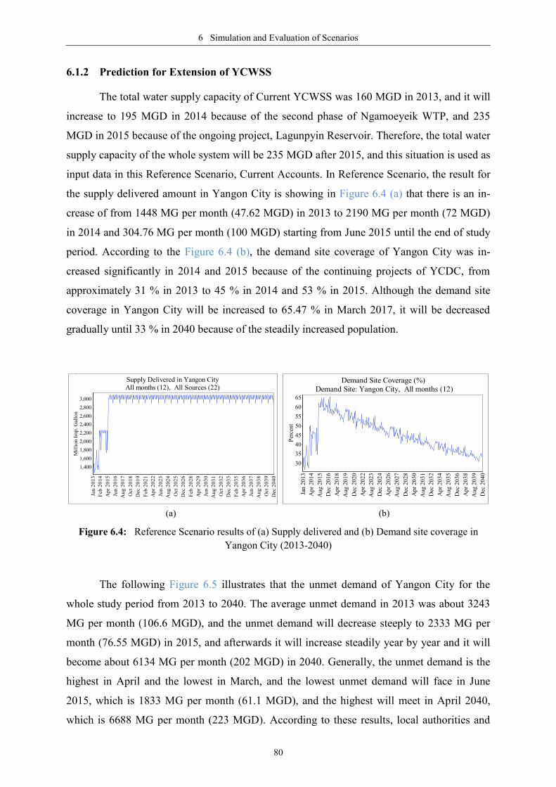
6 Simulation and Evaluation of Scenarios
80
6.1.2 Prediction for Extension of YCWSS
The total water supply capacity of Current YCWSS was 160 MGD in 2013, and it will
increase to 195 MGD in 2014 because of the second phase of Ngamoeyeik WTP, and 235
MGD in 2015 because of the ongoing project, Lagunpyin Reservoir. Therefore, the total water
supply capacity of the whole system will be 235 MGD after 2015, and this situation is used as
input data in this Reference Scenario, Current Accounts. In Reference Scenario, the result for
the supply delivered amount in Yangon City is showing in Figure 6.4 (a) that there is an in-
crease of from 1448 MG per month (47.62 MGD) in 2013 to 2190 MG per month (72 MGD)
in 2014 and 304.76 MG per month (100 MGD) starting from June 2015 until the end of study
period. According to the Figure 6.4 (b), the demand site coverage of Yangon City was in-
creased significantly in 2014 and 2015 because of the continuing projects of YCDC, from
approximately 31 % in 2013 to 45 % in 2014 and 53 % in 2015. Although the demand site
coverage in Yangon City will be increased to 65.47 % in March 2017, it will be decreased
gradually until 33 % in 2040 because of the steadily increased population.
(a) (b)
Figure 6.4: Reference Scenario results of (a) Supply delivered and (b) Demand site coverage in
Yangon City (2013-2040)
The following Figure 6.5 illustrates that the unmet demand of Yangon City for the
whole study period from 2013 to 2040. The average unmet demand in 2013 was about 3243
MG per month (106.6 MGD), and the unmet demand will decrease steeply to 2333 MG per
month (76.55 MGD) in 2015, and afterwards it will increase steadily year by year and it will
become about 6134 MG per month (202 MGD) in 2040. Generally, the unmet demand is the
highest in April and the lowest in March, and the lowest unmet demand will face in June
2015, which is 1833 MG per month (61.1 MGD), and the highest will meet in April 2040,
which is 6688 MG per month (223 MGD). According to these results, local authorities and
Reference Scenario
Supply Delivered in Yangon CityAll months (12), All Sources (22)
Jan
20
13
Feb
20
14
Ap
r 2
01
5
Jun
20
16
Au
g 2
01
7
Oct
20
18
Dec
20
19
Feb
20
21
Ap
r 2
02
2
Jun
20
23
Au
g 2
02
4
Oct
20
25
Dec
20
26
Feb
20
28
Ap
r 2
02
9
Jun
20
30
Au
g 2
03
1
Oct
20
32
Dec
20
33
Feb
20
35
Ap
r 2
03
6
Jun
20
37
Au
g 2
03
8
Oct
20
39
Dec
20
40
Mil
lio
n I
mp
. G
allo
n
3,000
2,800
2,600
2,400
2,200
2,000
1,800
1,600
1,400
Reference Scenario Demand Site Coverage (%)
Demand Site: Yangon City, All months (12)
Jan 2
013
Apr
2014
Aug 2
015
Dec
2016
Apr
2018
Aug 2
019
Dec
2020
Apr
2022
Aug 2
023
Dec
2024
Apr
2026
Aug 2
027
Dec
2028
Apr
2030
Aug 2
031
Dec
2032
Apr
2034
Aug 2
035
Dec
2036
Apr
2038
Aug 2
039
Dec
2040
Per
cent
65
60
55
50
45
40
35
30

6 Simulation and Evaluation of Scenarios
81
water managers of YCWSS should draw a plan to extend the current system for the unmet
demand problem of Yangon City. At present, YCDC and JICA are coordinating the imple-
mentation of water supply system development plan for Yangon City, and two river water
supply projects with a total capacity 240MGD are included in this plan. Since the results of
WEAP simulation are highlighted that 223 MGD for the future unmet demand for Yangon
City, it is obvious that these two projects of YCDC are necessary to implement in YCWSS.
Figure 6.5: Unmet demand of Yangon City in Reference Scenario (2013-2040)
In this Reference Scenario, the situations of supply sources in YCWSS, which are sur-
face water sources and ground water sources, can be evaluated by using the simulated results
of WEAP. The below Figure 6.6 describes that the graphs of the runoff flows from the five
catchments to their corresponding reservoirs of YCWSS for the study time horizon (2013-
2040). In these graphs, runoff from the catchment will decline remarkably in some dry years
like as 2020 and 2034. However, according to the simulated results of the reservoir storage
volumes and zones of reservoirs, WEAP is forecasted that storage volumes of all reservoirs in
YCWSS cannot be lower than the buffer zone until 2040, even though storage volumes of
Gyobyu reservoir will approach to the buffer zone in some years. The Figure 6.7 lists the
graphs for five reservoirs of YCWSS for the whole study projection starting from 2013 to the
end of this study, 2040. Therefore, it is noticeable that all reservoirs of YCWSS are reliable
for their operation until 2040 to supply their design water capacity to Yangon City via trans-
mission links.
Yangon City Unmet Demand in Yangon City
Scenario: Reference Scenario, All months (12)
Jan 2
013
Oct
2013
Aug 2
014
Jun 2
015
Apr
2016
Feb
2017
Dec
2017
Oct
2018
Aug 2
019
Jun 2
020
Apr
2021
Feb
2022
Dec
2022
Oct
2023
Aug 2
024
Jun 2
025
Apr
2026
Feb
2027
Dec
2027
Oct
2028
Aug 2
029
Jun 2
030
Apr
2031
Feb
2032
Dec
2032
Oct
2033
Aug 2
034
Jun 2
035
Apr
2036
Feb
2037
Dec
2037
Oct
2038
Aug 2
039
Jun 2
040
Mil
lion I
mp. G
allo
n
6,500
6,000
5,500
5,000
4,500
4,000
3,500
3,000
2,500
2,000

6 Simulation and Evaluation of Scenarios
82
(a) (b)
(c) (d)
(e)
Figure 6.6: Runoff flow from (a) Gyobyu (b) Hlawga (c) Phugyi (d) Ngamoeyeik (e) Lagunpyin
catchments to respective reservoirs of YCWSS (2013-2040)
(a) (b)
Reference Scenario Runoff Flow from Gyobyu Catchment to Gyobyu Reservoir
Reference Scenario, All months (12)
Jan
20
13
Ap
r 2
01
4
Sep
20
15
Feb
20
17
Jul
20
18
Dec
20
19
May
20
21
Oct
20
22
Mar
20
24
Au
g 2
02
5
Jan
20
27
Jun
20
28
No
v 2
02
9
Ap
r 2
03
1
Sep
20
32
Feb
20
34
Jul
20
35
Dec
20
36
May
20
38
Oct
20
39
Mil
lio
n I
mp
. G
allo
n6,000
5,000
4,000
3,000
2,000
1,000
0
Reference Scenario Runoff Flow from Hlawga Catchment to Hlawga Reservoir
Reference Scenario, All months (12)
Jan
20
13
Ap
r 2
01
4
Sep
20
15
Feb
20
17
Jul
20
18
Dec
20
19
May
20
21
Oct
20
22
Mar
20
24
Au
g 2
02
5
Jan
20
27
Jun
20
28
No
v 2
02
9
Ap
r 2
03
1
Sep
20
32
Feb
20
34
Jul
20
35
Dec
20
36
May
20
38
Oct
20
39
Mil
lio
n I
mp
. G
allo
n 4,000
3,000
2,000
1,000
0
Reference Scenario Runoff Flow from Phugyi Catchment to Phugyi Reservoir
Reference Scenario, All months (12)
Jan
20
13
May
20
14
Oct
20
15
Mar
20
17
Au
g 2
01
8
Jan
20
20
Jun
20
21
Dec
20
22
May
20
24
Oct
20
25
Mar
20
27
Au
g 2
02
8
Feb
20
30
Jul
20
31
Dec
20
32
May
20
34
Oct
20
35
Mar
20
37
Sep
20
38
Feb
20
40
Mil
lio
n I
mp
. G
allo
n
12,000
10,000
8,000
6,000
4,000
2,000
0
Reference Scenario Runoff Flow from Ngamoeyeik Catchment to Ngamoeyeik Reservoir
Reference Scenario, All months (12)
Jan
20
13
May
20
14
Oct
20
15
Mar
20
17
Au
g 2
01
8
Jan
20
20
Jun
20
21
Dec
20
22
May
20
24
Oct
20
25
Mar
20
27
Au
g 2
02
8
Feb
20
30
Jul
20
31
Dec
20
32
May
20
34
Oct
20
35
Mar
20
37
Sep
20
38
Feb
20
40
Mil
lio
n I
mp
. G
allo
n
70,000
60,000
50,000
40,000
30,000
20,000
10,000
0
Reference Scenario Runoff Flow from Lagunpyin Catchment to Lagunpyin Reservoir
Reference Scenario, All months (12)
Jan
20
13
May
20
14
Oct
20
15
Mar
20
17
Au
g 2
01
8
Jan
20
20
Jun
20
21
Dec
20
22
May
20
24
Oct
20
25
Mar
20
27
Au
g 2
02
8
Feb
20
30
Jul
20
31
Dec
20
32
May
20
34
Oct
20
35
Mar
20
37
Sep
20
38
Feb
20
40
Mil
lio
n I
mp
. G
allo
n
15,000
10,000
5,000
0
Storage Volume Top of Buffer Top of Conservation Top of Inactive
Reservoir Storage Volume and Zones of Gyobyu ReservoirScenario: Reference Scenario, All months (12)
Jan
20
13
Ap
r 2
01
4
Sep
20
15
Jan
20
17
Jun
20
18
Oct
20
19
Feb
20
21
Jul
20
22
No
v 2
02
3
Mar
20
25
Au
g 2
02
6
Dec
20
27
Ap
r 2
02
9
Sep
20
30
Jan
20
32
May
20
33
Oct
20
34
Feb
20
36
Jun
20
37
No
v 2
03
8
Mar
20
40
Mil
lio
n c
ub
ic m
etre
75
70
65
60
55
50
45
40
Storage Volume Top of Buffer Top of Conservation Top of Inactive
Reservoir Storage Volume and Zones of Hlawga ReservoirScenario: Reference Scenario, All months (12)
Jan
20
13
Ap
r 2
01
4
Sep
20
15
Jan
20
17
Jun
20
18
Oct
20
19
Feb
20
21
Jul
20
22
No
v 2
02
3
Mar
20
25
Au
g 2
02
6
Dec
20
27
Ap
r 2
02
9
Sep
20
30
Jan
20
32
May
20
33
Oct
20
34
Feb
20
36
Jun
20
37
No
v 2
03
8
Mar
20
40
Mil
lio
n c
ub
ic m
etre
55
50
45
40
35
30
25
20
15
10

6 Simulation and Evaluation of Scenarios
83
(c) (d)
(e)
Figure 6.7: Simulated reservoir storage volumes and zones of (a) Gyobyu (b) Hlawga (c) Phugyi (d)
Ngamoeyeik (e) Lagunpyin reservoirs of YCWSS (2013-2040)
The following Figure 6.8 represents the simulated results for future situations of
groundwater sources in YCWSS, and in these results, the main groundwater source for YCDC
tube wells is declining enormously due to the serious over-exploitation of groundwater, but
groundwater analysis for YCWSS needs to revise by using the more reliable data. In YCDC-
JICA study, it is pointed out that groundwater withdrawal amount is higher that groundwater
potential in Yangon City and it encourage to stop using groundwater in Yangon City.
Figure 6.8: Groundwater storage changes in different groundwater sources of YCWSS (2013-2040)
Storage Volume Top of Buffer Top of Conservation Top of Inactive
Reservoir Storage Volume and Zones of Phugyi Reservoir Scenario: Reference Scenario, All months (12)
Jan
20
13
Ap
r 2
01
4
Sep
20
15
Jan
20
17
Jun
20
18
No
v 2
01
9
Ap
r 2
02
1
Sep
20
22
Feb
20
24
Jul
20
25
Dec
20
26
Ap
r 2
02
8
Sep
20
29
Feb
20
31
Jul
20
32
Dec
20
33
May
20
35
Oct
20
36
Mar
20
38
Au
g 2
03
9
Mil
lio
n c
ub
ic m
etre
100
80
60
40
20
0
Storage Volume Top of Buffer Top of Conservation Top of Inactive
Reservoir Storage Volume and Zones of Ngamoeyeik ReservoirScenario: Reference Scenario, All months (12)
Jan
20
13
Ap
r 2
01
4
Sep
20
15
Jan
20
17
Jun
20
18
No
v 2
01
9
Ap
r 2
02
1
Sep
20
22
Feb
20
24
Jul
20
25
Dec
20
26
Ap
r 2
02
8
Sep
20
29
Feb
20
31
Jul
20
32
Dec
20
33
May
20
35
Oct
20
36
Mar
20
38
Au
g 2
03
9
Mil
lio
n c
ub
ic m
etre
200
150
100
50
Storage Volume Top of Buffer Top of Conservation Top of Inactive
Reservoir Storage Volume and Zones of Lagunpyin Reservoir Scenario: Reference Scenario, All months (12)
Jan
20
13
Ap
r 2
01
4
Sep
20
15
Jan
20
17
Jun
20
18
No
v 2
01
9
Ap
r 2
02
1
Sep
20
22
Feb
20
24
Jul
20
25
Dec
20
26
Ap
r 2
02
8
Sep
20
29
Feb
20
31
Jul
20
32
Dec
20
33
May
20
35
Oct
20
36
Mar
20
38
Au
g 2
03
9
Mil
lio
n c
ub
ic m
etre
180
160
140
120
100
80
60
40
20
0
Storage Volume Top of Buffer Top of Conservation Top of Inactive
Reservoir Storage Volume and Zones of Lagunpyin ReservoirScenario: Reference Scenario, All months (12)
Jan
20
13
Ap
r 2
01
4
Sep
20
15
Feb
20
17
Jul
20
18
Dec
20
19
May
20
21
Oct
20
22
Mar
20
24
Au
g 2
02
5
Jan
20
27
Jun
20
28
No
v 2
02
9
Ap
r 2
03
1
Sep
20
32
Feb
20
34
Jul
20
35
Dec
20
36
May
20
38
Oct
20
39
Mil
lio
n c
ub
ic m
etre
180
160
140
120
100
80
60
40
20
0
Groundwater Storage in Reference ScenarioSouth Dagon GWTP Thaephyu GWTP YCDC Tube Wells Yangon Pauk GWTP
Jan
20
13
No
v 2
01
3
Oct
20
14
Sep
20
15
Au
g 2
01
6
Jul
20
17
Jun
20
18
May
20
19
Ap
r 2
02
0
Mar
20
21
Feb
20
22
Jan
20
23
Dec
20
23
No
v 2
02
4
Oct
20
25
Sep
20
26
Au
g 2
02
7
Jul
20
28
Jun
20
29
May
20
30
Ap
r 2
03
1
Mar
20
32
Feb
20
33
Jan
20
34
Dec
20
34
No
v 2
03
5
Oct
20
36
Sep
20
37
Au
g 2
03
8
Jul
20
39
Jun
20
40
Mil
lio
n I
mp
. G
allo
n
90,000
80,000
70,000
60,000
50,000
40,000
30,000
20,000
10,000
0

6 Simulation and Evaluation of Scenarios
84
Therefore, the current situation of YCWSS can be predicted that there will be a huge
shortage in demand coverage and the unmet demand of Yangon City will be over 200 MGD
in the late 2030s. The current YCWSS mainly depends on the surface water from reservoirs,
which are seemed to be secure for the future whereas using groundwater source in Yangon
City will have problem in future because of its limited amount and other environmental im-
pacts. Moreover, external alternatives in the future, like as population growth and economic
development of the city, and climate change, can have an effect on the situation of YCWSS,
and these impacts will be discussed in the next section by simulating the different external
driven scenario for YCWSS.
6.2 Impacts of External driven scenarios
The following Figure 6.9 and Figure 6.10 show the demand coverage and the unmet
demand of Yangon City under four different external alternative scenarios, such as CC, HPG,
LPG and HLS scenarios, comparing with the Reference Scenario for the simulation period
2013 - 2040. In general, there will be significant negative impacts on water demand coverage
of Yangon City under HPG and HLS scenarios and large positive influence under LPG sce-
nario, whereas there is no effect under the CC scenario (see in Figure 6.9). Likewise, the un-
met demand amount in HPG and HLS will become higher gradually than that in Reference
Scenario, but that in LPG Scenario is noticeable lower (see in Figure 6.10). However, there is
no difference between the results of CC Scenario and Reference Scenario. The detail discus-
sion for the result data of these scenarios can be described in the following sub-sections.
Figure 6.9: Demand site coverage of Yangon under different external driven scenarios (2013-2040)
Demand Site Coverage (%) of Yangon CityCC Climate Change Scenario HLS Higher Living Standard Scenario HPG High Population Growth ScenarioLPG Low Population Growth Scenario Reference Scenario
Jan 2
013
Aug 2
013
Apr
2014
Dec
2014
Aug 2
015
Apr
2016
Dec
2016
Aug 2
017
Apr
2018
Dec
2018
Aug 2
019
Apr
2020
Dec
2020
Aug 2
021
Apr
2022
Dec
2022
Aug 2
023
Apr
2024
Dec
2024
Aug 2
025
Apr
2026
Dec
2026
Aug 2
027
Apr
2028
Dec
2028
Aug 2
029
Apr
2030
Dec
2030
Aug 2
031
Apr
2032
Dec
2032
Aug 2
033
Apr
2034
Dec
2034
Aug 2
035
Apr
2036
Dec
2036
Aug 2
037
Apr
2038
Dec
2038
Aug 2
039
Apr
2040
Dec
2040
Per
cent
65
60
55
50
45
40
35
30
25
20
15

6 Simulation and Evaluation of Scenarios
85
Figure 6.10: Unmet demand of Yangon City under different external driven scenarios (2013-2040)
6.2.1 High Population Growth - HPG Scenario
In this HPG Scenario, the population growth rate was used as 3.5 % instead of the
normal growth 2.5 % as in the Reference Scenario, and the simulation results for demand site
coverage of Yangon City show that both scenarios have similar fluctuation but the results of
HPG Scenario is much lower than that of Reference Scenario (see in Figure 6.9). The lowest
demand coverage amount in HPG scenario will be only 14 % in April 2040 whereas that in
Reference Scenario will be about 31 % in April 2040. As a result of this low demand cover-
age problem, the unmet demand of Yangon City in this scenario will reach 10796 MG per
month (360 MGD) in April 2040 as the maximum amount under this scenario (see in Figure
6.10).
Thus, YCWSS can encounter a huge water shortage problem if the population growth
in Yangon City was increased due to the urbanization and industrialization of the urban region
together with the migration of people from rural regions.
6.2.2 Low Population Growth - LPG Scenario
The population growth rate in this LPG Scenario was estimated as 1.5 %, and the
demand coverage results of Yangon City in WEAP simulation provide that the results of LPG
Scenario is substantially lower than that of Reference Scenario according to the Figure 6.9. In
LPG scenario, even the demand coverage amount will be 40.3 % in April 2040, but that in
Reference Scenario will be about 31 % in that month. Similarly, the unmet demand of Yan-
Unmet Demand in Yangon CityCC Climate Change Scenario HLS Higher Living Standard Scenario HPG High Population Growth ScenarioLPG Low Population Growth Scenario Reference Scenario
Jan 2
013
Aug 2
013
Apr
2014
Dec
2014
Aug 2
015
Apr
2016
Dec
2016
Aug 2
017
Apr
2018
Dec
2018
Aug 2
019
Apr
2020
Dec
2020
Aug 2
021
Apr
2022
Dec
2022
Aug 2
023
Apr
2024
Dec
2024
Aug 2
025
Apr
2026
Dec
2026
Aug 2
027
Apr
2028
Dec
2028
Aug 2
029
Apr
2030
Dec
2030
Aug 2
031
Apr
2032
Dec
2032
Aug 2
033
Apr
2034
Dec
2034
Aug 2
035
Apr
2036
Dec
2036
Aug 2
037
Apr
2038
Dec
2038
Aug 2
039
Apr
2040
Dec
2040
Mil
lion I
mp. G
allo
n
11,000
10,000
9,000
8,000
7,000
6,000
5,000
4,000
3,000
2,000

6 Simulation and Evaluation of Scenarios
86
gon City in this scenario will be 4436 MG per month (148 MGD) in April 2040 as the maxi-
mum unmet demand for the whole scenario while Reference Scenario will be unmet about
223 MGD (see in Figure 6.10).
As a result, YCWSS can improve its water supply capacity if the population growth
rate in Yangon City was altered slower like as other urbanized mega cities.
6.2.3 Higher Living Standards - HLS Scenario
In this HLS Scenario, it was assumed that the water consumption rate would become
rise together with the economic growth of the city because of higher living standards. In
Asian countries, the higher the living standards and the economic growth, the higher the water
consumption because of oriental living style, for example, wet sanitation. Future service tar-
get of YCDC for water consumption rate, 30 gpcd in 2013 to 40 gpcd in 2040, was used to
analyse the impact of this changes. The simulation results for demand site coverage of Yan-
gon City are the lowest in this scenario, which is 13.86 % in April 2040, comparing with all
other scenarios (see in Figure 6.9). The unmet demand of Yangon City in this scenario will
gain the highest peak, which is 11157 MG per month (372 MGD) in April 2040 (see in Figure
6.10).
Therefore, YCWSS can face a large water deficit problem if the higher living stand-
ards in Yangon City were occurred due to the change of economic development pattern in
Yangon City.
6.2.4 Climate Change Scenario - CC Scenario
In this CC Scenario, GCM: CMIP5 full set climate data with RCP6.0 scenario was
used to study the impacts of climate change in Yangon City, and the simulated results for both
demand site coverage and unmet demand of Yangon City under this scenario have exactly the
same trends as Reference Scenario (see in Figure 6.9 and Figure 6.10).
Hence, these results demonstrated that there is no impact of climate change on this
YCWSS model using this RCP6.0 scenario climate change model data, and these results also
highlighted that the climate data that used in Reference Scenario, that was cycled the histori-
cal climate data (1991-2013), are reliable to study the future of water supply-demand system.
The other climate change data for different scenarios from different climate change models
should use for further study about the climate change impact on this YCWSS.

6 Simulation and Evaluation of Scenarios
87
6.3 Advantages of Management Scenarios
Regarding to solve the negative impacts of external alternatives in YCWSS, four sce-
narios for management options, two DSM scenarios and 2 SSM scenarios, to practise in the
system will be explored to figure out their advantages on water supply coverage and unmet
demand of Yangon City. Comparing the results of these scenarios in demand site coverage
and unmet demand of Yangon City are illustrated in Figure 6.11 and Figure 6.12. These
graphs show that all management options have significant positive impacts on the improve-
ment of YCWSS, and 100% demand coverage can achieve under SSM-ASS Scenario starting
from 2035. However, SSM-NRWC option is the best effective management option from eco-
nomical and environmental points of view because Yangon can get maximum coverage 81%
by implementing NRW control management plan without using big investment. Due to the
SSM-NRWC option, demand coverage in Yangon City will improve about 20 % of the Refer-
ence Scenario result for the whole study period, and the average unmet demand of Yangon
City under this scenario can reduce about 41 % of the Reference scenario. Similarly, demand
coverage of Yangon City under DSM-WPP Scenario can improve 10 % of that under Refer-
ence Scenario, and the unmet demand will fall about 35 % of that under Reference Scenario.
Under DSM-SWS option, the sustainable water source, rainwater was used to study the alter-
native technology in water supply system, and the remarkable effect on water demand cover-
age in the rainy season, and in the mid of rainy season, that value is more than 10 % of the
data under Reference Scenario. The improvement of water supply service in each scenario
will be discussed in their respective sub-section.
Figure 6.11: Demand Coverage of Yangon City under management scenarios (2013-2040)
Demand Site Coverage (%) in Yangon CityDSM_SWS Sustainable Water Source Scenario DSM_WPP Water Pricing Policy ScenarioReference Scenario SSM_ASS Alternative Supply Source ScenarioSSM_NRWC Non-Revenue Water Control Scenario
Jan 2
013
Aug 2
013
Apr
2014
Dec
2014
Aug 2
015
Apr
2016
Dec
2016
Aug 2
017
Apr
2018
Dec
2018
Aug 2
019
Apr
2020
Dec
2020
Aug 2
021
Apr
2022
Dec
2022
Aug 2
023
Apr
2024
Dec
2024
Aug 2
025
Apr
2026
Dec
2026
Aug 2
027
Apr
2028
Dec
2028
Aug 2
029
Apr
2030
Dec
2030
Aug 2
031
Apr
2032
Dec
2032
Aug 2
033
Apr
2034
Dec
2034
Aug 2
035
Apr
2036
Dec
2036
Aug 2
037
Apr
2038
Dec
2038
Aug 2
039
Apr
2040
Dec
2040
Per
cent
100
90
80
70
60
50
40
30

6 Simulation and Evaluation of Scenarios
88
Figure 6.12: Unmet demand of Yangon City under management scenarios (2013-2040)
6.3.1 1st DSM - Water Pricing Policy (WPP) Scenario
In this DSM-WPP Scenario, the DSM saving was used as 20 % because of the changes
of water pricing policy that is altering the water pricing system from fixed water-pricing to
tiered water-pricing and increasing the water price to reduce the water demand of Yangon
City. The Figure 6.11 provides the information for demand site coverage of Yangon City that
is relatively higher than the default scenario with the average difference is about 11 % and
both scenarios have the same trend from the beginning to the end of the study period. The
high water coverage in this scenarios will be 81.8 % in March 2017 whereas 65.5 % in the
default scenario. Although the difference between these two scenarios will be becoming
smaller year after year, the diffidence amount still remains 10 % at the end of the study, De-
cember 2040. The maximum unmet demand in DSM - WPP Scenario is 4898 MG per month
(158 MGD) in May 2040, and the same time 6679 MG per month (215 MGD) in Reference
Scenario (see in Figure 6.12).
On one hand, it is obvious that water pricing policy change can provide an advantage
for the improvement of the water supply service, and on the other hand, this change can in-
crease the income of water authorities.
6.3.2 2nd
DSM - Sustainable Water Source (SWS) Scenario
For this DSM-SWS option, RWH was used to initiate in the demand side of YCWSS
by assuming only 1 m2 harvested area and 1 m
3 storage capacity for each citizen who is in-
creased after 2013. According to the Figure 6.11, the demand site coverage of Yangon City
Unmet Demand in Yangon CityDSM_SWS Sustainable Water Source Scenario DSM_WPP Water Pricing Policy ScenarioReference Scenario SSM_ASS Alternative Supply Source ScenarioSSM_NRWC Non-Revenue Water Control Scenario
Jan 2
013
Aug 2
013
Apr
2014
Dec
2014
Aug 2
015
Apr
2016
Dec
2016
Aug 2
017
Apr
2018
Dec
2018
Aug 2
019
Apr
2020
Dec
2020
Aug 2
021
Apr
2022
Dec
2022
Aug 2
023
Apr
2024
Dec
2024
Aug 2
025
Apr
2026
Dec
2026
Aug 2
027
Apr
2028
Dec
2028
Aug 2
029
Apr
2030
Dec
2030
Aug 2
031
Apr
2032
Dec
2032
Aug 2
033
Apr
2034
Dec
2034
Aug 2
035
Apr
2036
Dec
2036
Aug 2
037
Apr
2038
Dec
2038
Aug 2
039
Apr
2040
Dec
2040
Mil
lion I
mp. G
allo
n
6,500
6,000
5,500
5,000
4,500
4,000
3,500
3,000
2,500
2,000
1,500
1,000
500
0

6 Simulation and Evaluation of Scenarios
89
under this option will becoming significant in 2030s because the results in the rainy season
under this scenario can be about 10 % more than that under Reference Scenario in those years.
For instance, the demand coverage in this scenario will be 48.27 % in July 2037 and 45.33 %
in August 40 while these in Reference Scenario will be 36.4 % and 34.78 % respectively.
Meanwhile, the unmet demand under this DSM-SWS Scenario will descend to 4387 MG per
month (141.5 MGD) in July 2037 and 4852 MG per month (156 MGD) in Aug 2040, but
Reference Scenario will have 5394 MG per month (174 MGD) and 5788 MG per month (187
MGD) (see in Figure 6.12).
According to these results, RWH can help to improve the water supply system effec-
tively into a certain level and YCDC should encourage installing this facilities in the demand
sites to reduce the water demand from the network.
6.3.3 1st SSM – NRW Control (NRWC) Scenario
For this SSM-NRWC option, EDWS will carry out to reduce the water losses in the
system by implementing different strategies, such as leakage control plan, pipeline rehabilita-
tion plan, connection control plan, and water-meter reinstallation plan etc., to reach the future
target for NRW that is to reach 15 % in 2040. For this scenario, future target data of YCDC-
JICA master plan were used to study the effect of NRWC program. According to the results,
this scenario can raise the water supply service enormously, for example, the demand site
coverage in this scenario will have 61.5 %, and in Reference Scenario will have 31 % at the
end of simulation period, December 2040 (see in Figure 6.11). In December 2040, the unmet
demand in this scenario will be 3399 MG per month (109 MGD), whilst 6094 MG per month
(196.5 MGD) in Reference Scenario (see in Figure 6.12).
Simulation for this SSM-NRWC showed that the water supply service in YCWSS
could improve doubled by controlling NRW with low investment and energy. Moreover,
NRW controlling not only can improve the quantity of the supply water but also can upgrade
the supply water quality without disturbing environment. Therefore, NRWC option is the best
strategy for the improvement of YCWSS.
6.3.4 2nd
SSM - Alternative Supply Source (ASS) Scenario
In YCDC-JICA Master Plan, it is mentioned that the alterations of water supply
sources in YCWSS to introduce river water sources and to cease the groundwater source. Two
new river water supply projects will implement for future increased demand of Yangon City.

6 Simulation and Evaluation of Scenarios
90
According to the results for this scenario from Figure 6.11 and Figure 6.12, the demand site
coverage of Yangon City will achieve 100 % after January 2035, and there will not be unmet
demand after 2034, even though the unmet demand in December 2034 can occur 1867 MG
per month (60 MGD).
It is evidence that these new water supply projects for YCWSS are essential to attain
100 % reliable water supply service in the future.
6.4 Strategic Development Options for Future YCWSS
Since the main objective of YCWSS is to distribute the adequate water for city dwell-
ers, water managers and decision maker of YCDC should formulate the development for
YCWSS in order to contribute to socioeconomic development of Yangon City. Therefore,
YCWSS should be developed not only for the business-as-usual case, but also for the worst
cases by using the best management strategies. WEAP is the best tool to analyse the impacts
of different management options under different situations. Moreover, WEAP can operate
easily to integrate these different options and different situations to find out the worst situa-
tion and the best solution for the system. The following Figure 6.13 and Figure 6.14 illustrate
the demand coverage percent and unmet demand in Yangon City that will encounter in April
2040 under different scenario. According to these figures, HPG and HLS scenarios can affect
the highest negative impact on the system, and SSM-AAS option is the best option to gain
100 % system reliability. Besides, SSM-NRWC option can achieve significant positive effect
on the system, which is double of Reference Scenario, and DSM-WPP option also can give
moderate advantage to the system.
Figure 6.13: Comparison of water coverage in Yangon City under different scenarios (April, 2040)
Yangon City
Demand Site Coverage (%) of Yangon City in April, 2040
CC
Cli
mate
Ch
an
ge S
cen
ari
o
DS
M_
SW
S S
ust
ain
ab
le W
ate
r S
ou
rce S
cen
ari
o
DS
M_
WP
P W
ate
r P
ricin
g P
oli
cy
Scen
ari
o
HL
S H
igh
er
Liv
ing
Sta
nd
ard
Scen
ari
o
HP
G H
igh
Po
pu
lati
on
Gro
wth
Scen
ari
o
LP
G L
ow
Po
pu
lati
on
Gro
wth
Scen
ari
o
Refe
ren
ce S
cen
ari
o
SS
M_
AS
S A
ltern
ati
ve S
up
ply
So
urc
e S
cen
ari
o
SS
M_
NR
WC
No
n-R
ev
en
ue W
ate
r C
on
tro
l S
cen
ari
o
Perc
en
t
100
80
60
40
20
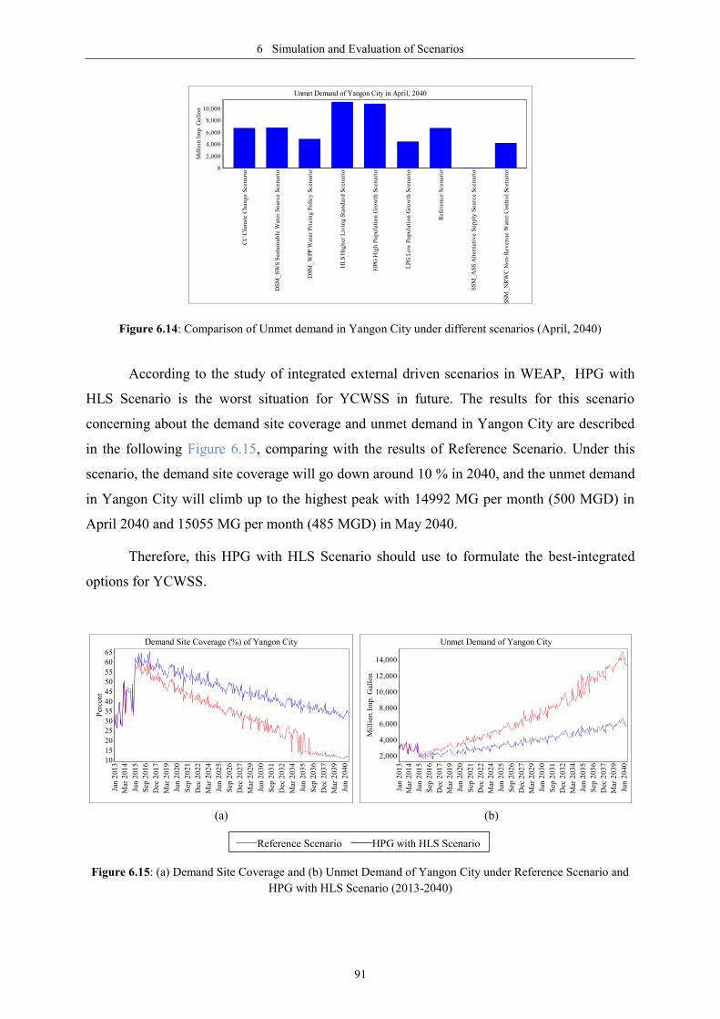
6 Simulation and Evaluation of Scenarios
91
Figure 6.14: Comparison of Unmet demand in Yangon City under different scenarios (April, 2040)
According to the study of integrated external driven scenarios in WEAP, HPG with
HLS Scenario is the worst situation for YCWSS in future. The results for this scenario
concerning about the demand site coverage and unmet demand in Yangon City are described
in the following Figure 6.15, comparing with the results of Reference Scenario. Under this
scenario, the demand site coverage will go down around 10 % in 2040, and the unmet demand
in Yangon City will climb up to the highest peak with 14992 MG per month (500 MGD) in
April 2040 and 15055 MG per month (485 MGD) in May 2040.
Therefore, this HPG with HLS Scenario should use to formulate the best-integrated
options for YCWSS.
(a) (b)
Figure 6.15: (a) Demand Site Coverage and (b) Unmet Demand of Yangon City under Reference Scenario and
HPG with HLS Scenario (2013-2040)
Yangon City
Unmet Demand of Yangon City in April, 2040
CC
Cli
mate
Ch
an
ge S
cen
ari
o
DS
M_
SW
S S
ust
ain
ab
le W
ate
r S
ou
rce S
cen
ari
o
DS
M_
WP
P W
ate
r P
ricin
g P
oli
cy
Scen
ari
o
HL
S H
igh
er
Liv
ing
Sta
nd
ard
Scen
ari
o
HP
G H
igh
Po
pu
lati
on
Gro
wth
Scen
ari
o
LP
G L
ow
Po
pu
lati
on
Gro
wth
Scen
ari
o
Refe
ren
ce S
cen
ari
o
SS
M_
AS
S A
ltern
ati
ve S
up
ply
So
urc
e S
cen
ari
o
SS
M_
NR
WC
No
n-R
ev
en
ue W
ate
r C
on
tro
l S
cen
ari
o
Mil
lio
n I
mp
. G
all
on 10,000
8,000
6,000
4,000
2,000
0
HPG with HLS Scenario Reference Scenario
Demand Site Coverage (%) of Yangon City
Jan
20
13
Mar
20
14
Jun
20
15
Sep
20
16
Dec
20
17
Mar
20
19
Jun
20
20
Sep
20
21
Dec
20
22
Mar
20
24
Jun
20
25
Sep
20
26
Dec
20
27
Mar
20
29
Jun
20
30
Sep
20
31
Dec
20
32
Mar
20
34
Jun
20
35
Sep
20
36
Dec
20
37
Mar
20
39
Jun
20
40
Per
cen
t
65
60
55
50
45
40
35
30
25
20
15
10
HPG with HLS Scenario Reference Scenario
Unmet Demand of Yangon City
Jan
20
13
Mar
20
14
Jun
20
15
Sep
20
16
Dec
20
17
Mar
20
19
Jun
20
20
Sep
20
21
Dec
20
22
Mar
20
24
Jun
20
25
Sep
20
26
Dec
20
27
Mar
20
29
Jun
20
30
Sep
20
31
Dec
20
32
Mar
20
34
Jun
20
35
Sep
20
36
Dec
20
37
Mar
20
39
Jun
20
40
Mil
lio
n I
mp
. G
allo
n
14,000
12,000
10,000
8,000
6,000
4,000
2,000
Reference Scenario HPG with HLS Scenario
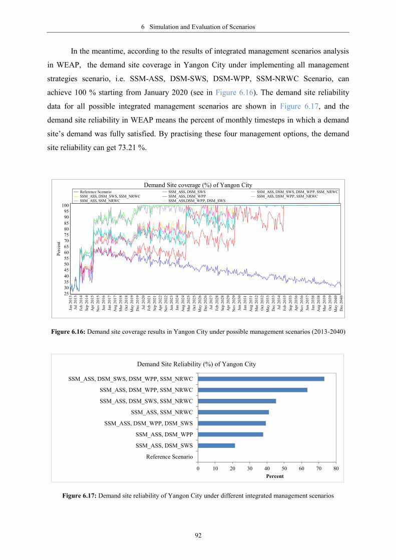
6 Simulation and Evaluation of Scenarios
92
In the meantime, according to the results of integrated management scenarios analysis
in WEAP, the demand site coverage in Yangon City under implementing all management
strategies scenario, i.e. SSM-ASS, DSM-SWS, DSM-WPP, SSM-NRWC Scenario, can
achieve 100 % starting from January 2020 (see in Figure 6.16). The demand site reliability
data for all possible integrated management scenarios are shown in Figure 6.17, and the
demand site reliability in WEAP means the percent of monthly timesteps in which a demand
site’s demand was fully satisfied. By practising these four management options, the demand
site reliability can get 73.21 %.
Figure 6.16: Demand site coverage results in Yangon City under possible management scenarios (2013-2040)
Figure 6.17: Demand site reliability of Yangon City under different integrated management scenarios
Demand Site coverage (%) of Yangon CityReference Scenario SSM_ASS, DSM_SWS SSM_ASS, DSM_SWS, DSM_WPP, SSM_NRWCSSM_ASS, DSM_SWS, SSM_NRWC SSM_ASS, DSM_WPP SSM_ASS, DSM_WPP, SSM_NRWCSSM_ASS, SSM_NRWC SSM_ASS,DSM_WPP, DSM_SWS
Jan
20
13
Jul
20
13
Feb
20
14
Sep
20
14
Ap
r 2
01
5
No
v 2
01
5
Jun
20
16
Jan
20
17
Au
g 2
01
7
Mar
20
18
Oct
20
18
May
20
19
Dec 2
01
9
Jul
20
20
Feb
20
21
Sep
20
21
Ap
r 2
02
2
No
v 2
02
2
Jun
20
23
Jan
20
24
Au
g 2
02
4
Mar
20
25
Oct
20
25
May
20
26
Dec 2
02
6
Jul
20
27
Feb
20
28
Sep
20
28
Ap
r 2
02
9
No
v 2
02
9
Jun
20
30
Jan
20
31
Au
g 2
03
1
Mar
20
32
Oct
20
32
May
20
33
Dec 2
03
3
Jul
20
34
Feb
20
35
Sep
20
35
Ap
r 2
03
6
No
v 2
03
6
Jun
20
37
Jan
20
38
Au
g 2
03
8
Mar
20
39
Oct
20
39
May
20
40
Dec 2
04
0
Per
cent
100
95
90
85
80
75
70
65
60
55
50
45
40
35
30
25
0 10 20 30 40 50 60 70 80
Reference Scenario
SSM_ASS, DSM_SWS
SSM_ASS, DSM_WPP
SSM_ASS, DSM_WPP, DSM_SWS
SSM_ASS, SSM_NRWC
SSM_ASS, DSM_SWS, SSM_NRWC
SSM_ASS, DSM_WPP, SSM_NRWC
SSM_ASS, DSM_SWS, DSM_WPP, SSM_NRWC
Percent
Demand Site Reliability (%) of Yangon City
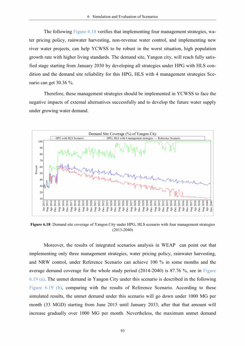
6 Simulation and Evaluation of Scenarios
93
The following Figure 6.18 verifies that implementing four management strategies, wa-
ter pricing policy, rainwater harvesting, non-revenue water control, and implementing new
river water projects, can help YCWSS to be robust in the worst situation, high population
growth rate with higher living standards. The demand site, Yangon city, will reach fully satis-
fied stage starting from January 2030 by developing all strategies under HPG with HLS con-
dition and the demand site reliability for this HPG, HLS with 4 management strategies Sce-
nario can get 30.36 %.
Therefore, these management strategies should be implemented in YCWSS to face the
negative impacts of external alternatives successfully and to develop the future water supply
under growing water demand.
Figure 6.18: Demand site coverage of Yangon City under HPG, HLS scenario with four management strategies
(2013-2040)
Moreover, the results of integrated scenarios analysis in WEAP can point out that
implementing only three management strategies, water pricing policy, rainwater harvesting,
and NRW control, under Reference Scenario can achieve 100 % in some months and the
average demand coverage for the whole study period (2014-2040) is 87.76 %, see in Figure
6.19 (a). The unmet demand in Yangon City under this scenario is described in the following
Figure 6.19 (b), comparing with the results of Reference Scenario. According to these
simulated results, the unmet demand under this scenario will go down under 1000 MG per
month (33 MGD) starting from June 2015 until January 2033, after that that amount will
increase gradually over 1000 MG per month. Nevertheless, the maximum unmet demand
Demand Site Coverage (%) of Yangon CityHPG with HLS Scenario HPG, HLS with 4 management strategies Reference Scenario
Jan 2
013
Aug 2
013
Apr
2014
Dec
2014
Aug 2
015
Apr
2016
Dec
2016
Aug 2
017
Apr
2018
Dec
2018
Aug 2
019
Apr
2020
Dec
2020
Aug 2
021
Apr
2022
Dec
2022
Aug 2
023
Apr
2024
Dec
2024
Aug 2
025
Apr
2026
Dec
2026
Aug 2
027
Apr
2028
Dec
2028
Aug 2
029
Apr
2030
Dec
2030
Aug 2
031
Apr
2032
Dec
2032
Aug 2
033
Apr
2034
Dec
2034
Aug 2
035
Apr
2036
Dec
2036
Aug 2
037
Apr
2038
Dec
2038
Aug 2
039
Apr
2040
Dec
2040
Per
cent
100
90
80
70
60
50
40
30
20
10

6 Simulation and Evaluation of Scenarios
94
under this scenario will be 2361 MG per month (78.7 MGD) in April 2040, which is much
more lower than the capacity of two new water supply projects of YCDC, Kokkowa River
Project with total capacity 240 MGD and Toe River Project Project with total capacity 180
MGD. As a result of this finding, water planner and decision makers of YCDC should revise
these new projects concerning with capacity and time horizon of the projects.
(a) (b)
Figure 6.19: (a) Demand Site Coverage and (b) Unmet Demand of Yangon City under Reference Scenario and 3
Strategies w/o new project Scenario (2013-2040)
In conclusion, management strategies studied in this thesis are significantly effective
on the development of YCWSS for the future water demand. This analysis pointed out that
implementing all strategies in the system can encounter well the worst situation in the future,
such as high population growth rate, high water consumption rate. Moreover, implementing
only three strategies without implementing new projects can adapt the Reference Scenario
situation effectively for the whole simulation period (2014-2040).
3 strategies w/o New Projects ScenarioReference Scenario
Demand Site Coverage (%) of Yangon City
Jan
20
13
Ap
r 2
01
4
Au
g 2
01
5
Dec
20
16
Ap
r 2
01
8
Au
g 2
01
9
Dec
20
20
Ap
r 2
02
2
Au
g 2
02
3
Dec
20
24
Ap
r 2
02
6
Au
g 2
02
7
Dec
20
28
Ap
r 2
03
0
Au
g 2
03
1
Dec
20
32
Ap
r 2
03
4
Au
g 2
03
5
Dec
20
36
Ap
r 2
03
8
Au
g 2
03
9
Dec
20
40
Per
cen
t
100
90
80
70
60
50
40
30
3 strategies w/o New Projects ScenarioReference Scenario
Unmet Demand of Yangon City
Jan
20
13
Ap
r 2
01
4
Au
g 2
01
5
Dec
20
16
Ap
r 2
01
8
Au
g 2
01
9
Dec
20
20
Ap
r 2
02
2
Au
g 2
02
3
Dec
20
24
Ap
r 2
02
6
Au
g 2
02
7
Dec
20
28
Ap
r 2
03
0
Au
g 2
03
1
Dec
20
32
Ap
r 2
03
4
Au
g 2
03
5
Dec
20
36
Ap
r 2
03
8
Au
g 2
03
9
Dec
20
40
Mil
lio
n I
mp
. G
allo
n
6,000
5,000
4,000
3,000
2,000
1,000
0
Reference Scenario 3 Strategies w/o new project Scenario

7 Discussions, Conclusions, and Recommendations
95
7 Discussions, Conclusions and Recommendations
7.1 Discussions and Conclusions
The overall objective of this study was to develop Water Evaluation And Planning
(WEAP) model for the simulation of current water supply system of Yangon City and for the
evaluation of different external changes scenarios and different water management strategies
for the future water supply against the growing water demand. In this study, external driven
scenarios under different population growth rate, higher water consumption rate, and climate
change, were constructed to reflect the impact on future trends of water supply sources and a
demand site, Yangon City. Moreover, management scenarios under both demand side and
supply side were constructed by taking into account the different operating policies and strat-
egies that may affect water demand and water supply. This study mainly focused on the water
demand coverage and unmet demand of Yangon City for long-term planning of YCWSS, and
the current accounts year was used as 2013 to simulate the study time horizon from 2014 until
2040.
This study used only one demand site, Yangon City, with aggregate method to analyse
the water availability in city level. Annual demand with monthly variation method was used
to determine the monthly water demand of Yangon City. Since there was no measured data
for monthly demand variation of Yangon City, the monthly water consumption data derived
from water bill income of YCDC was used to calculate the demand monthly variation. Con-
sequently, the result of this model has been influenced by this empirical data, having the low-
est water demand on March due to the financial management policy for the budget year in
YCDC and in Myanmar.
This study applied Rainfall Runoff (Simplified Coefficient) method to generate runoff
from rainfall, and the weakness of this method is not taking into account some hydrological
complex processes such as infiltration, percolation, and runoff concentration time etc. Thus,
the results of WEAP model was illustrated that the simulated reservoir storage volumes were
larger than the observed volumes of the reservoirs and the time intervals of the highest and
lowest water levels of the reservoirs in model simulated results were earlier than that in actual
cases. In this study, groundwater was simulated assuming possible data in some parameters
due to the lack of proper documents and reliable research paper. Similarly, rivers that will use
in future water supply projects for Yangon City were simulated by using minimum flow data
of these rivers from the flow measurement reports of MoAI.

7 Discussions, Conclusions, and Recommendations
96
In this study, Reference Scenario was created using current accounts data to evaluate
the current water supply- system of Yangon City and its future trends in both supply sources
and demand sites. According to the analysis of Reference Scenario, the following main results
can be discussed.
It was verified that the average demand coverage of Yangon City in 2013 was about
31 % and the supply delivered amount to Yangon City in 2013 was 47.94 MGD.
Therefore, YCWSS could supply water only one-third of city dwellers in 2013.
It was noticeable that the average demand coverage of Yangon City would jump to
about 46% in 2014 because of the 2nd
phase of Ngamoeyeik WTP project, and go up
to about 60% in 2016 because of Lagunpyin water supply project.
However, the results pointed out that the average demand coverage of Yangon City
will fall gradually until to reach about 33% in 2040.
It was remarkable that the average unmet demand of Yangon City in 2040 will be 202
MGD and the maximum unmet demand will be 223 MGD in April 2040. Thus,
YCWSS will be needed to extend by implementing new projects to improve the water
availability in Yangon City.
It was obvious that the surface water sources and the reservoirs of YCWSS will oper-
ate well until 2040, but the groundwater source of YCDC tube wells will be exhausti-
ble at the end of 2040.
In this study, four external driven scenarios and four management options were creat-
ed to analyse the impacts of external alternatives on YCWSS and the benefits of water man-
agement strategies for the water availability of Yangon City. Based on these different scenari-
os analysis data, the following facts can be extracted.
In High Population Growth Scenario, the demand coverage of Yangon City will de-
cline considerably comparing with the results of Reference Scenario, the average cov-
erage in 2040 will be 23%, and the average unmet demand in 2040 will be 300 MGD.
In Low Population Growth Scenario, the demand coverage of Yangon City will incline
markedly, and the average coverage in 2040 will get 42% and the average unmet de-
mand in 2040 will become 133 MGD.
In Higher Living Standards Scenario, there will be a noticeable negative impact on the
demand coverage of Yangon City, and the average water coverage in 2040 will get on-
ly 21% and the average unmet demand will rise until 314 MGD.

7 Discussions, Conclusions, and Recommendations
97
In Climate Change Scenario using GCM: CMIP5 full set climate data for RCP 6.0
scenario, there will be no effect on the water demand coverage of Yangon City getting
exactly the same results as Reference Scenario. The average demand coverage under
this scenario will be 33%, and the unmet demand in Yangon City will be 202 MGD.
In DSM - Water Pricing Policy Scenario, the demand coverage of Yangon City will
improve moderately to get the average demand coverage in 2040 is 40%, and the av-
erage unmet demand in 2040 is 145 MGD.
In DSM - Sustainable Water Source Scenario introducing rainwater harvesting to pub-
lic, the demand coverage of Yangon will be affected marginally and the average wa-
ter-demand coverage and the average unmet demand of Yangon City will become
36% and 192 MGD in 2040.
In SSM - NRW Control Scenario, there will show huge improvement in demand cov-
erage of Yangon City giving 61% for the average coverage in 2040 and 118 MGD for
the average unmet demand in 2040.
In SSM - Alternative Supply Source Scenario considering the two new water supply
projects from rivers and abandoning Groundwater sources, the demand coverage will
achieve the reliable stage by providing the average water-demand coverage of Yangon
City in 2040 will be 100% together with no unmet demand.
In this study, strategic development options for YCWSS to adapt the external alterna-
tives was analysed by integrating these different scenarios, and this adaptation analysis illu-
minated two important deductions regarding the improvement of YCWSS.
As a first deduction, integrating all management options that were discussed in this
study can adapt in the worst situation of Yangon City in future that is Yangon City will have
high population growth rate and higher water consumption rate because of economic growth
and higher living standards. According to the simulation result for HPG, HLS with four man-
agement strategies will obtain 100% demand coverage with no unmet demand situation in
2040.
As a second one, implementing three water management options without implement-
ing any extension and any new projects in the system under the current situation of YCWSS
can adapt well in the future until 2040. The simulated results for three strategies without new
projects scenario under the current accounts highlighted that the average demand coverage in
Yangon City can get 80% in 2040 accompanied with the unmet demand 50 MGD.

7 Discussions, Conclusions, and Recommendations
98
To be concluded, water pricing policy and NRW control are the two main keys to im-
prove the situation of YCWSS effectively from economical and environmental point of views.
Both management strategies have multi-advantages, for example, practising water pricing
policy not only control the public water consumption but also help to get a higher income in
water authorities. Similarly, NRW control can improve the water supply service both in quan-
titatively and qualitatively. Moreover, RWH can be considered a feasible water management
strategy in urban areas because RWH in urban areas can reduce not only the demand on water
supply facilities but also the demand on urban drainage system controlling the runoff and re-
ducing the urban flood. The result of this study confirmed that water managers and local au-
thorities of YCDC should formulate urgently these sustainable water management options for
YCWSS until to achieve the future targets and revised study for the implementation of new
water supply projects should be done.
7.2 Recommendations
This study clearly recommended that WEAP is powerful in evaluating the current situ-
ation and future options in water supply system. WEAP can evaluate all aspects of the water
system including rainfall-runoff, demand, supply, streamflow, groundwater, quality, and fi-
nance. WEAP can support results of the analysis on many spatial and temporal levels, such as
all or selected demand sites, all or selected supply sources, yearly long-time data, monthly
long-time data, monthly average, and selected years, showing in several formats such as
charts, tables, and maps. One of the strengths of WEAP is that additional or more accurate
data can be added directly to the developed model and simulation can be performed in a few
minutes. For example, a water quality analysis or financial analysis can be done very easily
with this YCWSS-WEAP model. WEAP model is based on a well-structured approach, and
that ensures fast in model development, ease in precise-analysis, and flexible in scenarios cre-
ation. In this study, WEAP could assist water planners and policy makers in decision making
for future management of the water supply-demand system. Another advantage of the WEAP
model is the support from the developers in terms of publications, tutorial, user guide, discus-
sion in user forum and software free-support to governmental and academic users from devel-
oping countries.
The application of WEAP in YCWSS demonstrated the advantages of some integrated
water management strategies for the impacts of external alternatives but also pointed out sev-
eral requirements to understand deeply for future changes and management options in

7 Discussions, Conclusions, and Recommendations
99
YCWSS. Based on these requirements, the following potential useful recommendations are
suggested.
Institutional policy and the participation of the local community should combine to
achieve the implementation of management strategies, such as RWH harvesting, NRW
control plan, and water-pricing policy successfully.
Local authorities should initiate laws and regulations concerning about these manage-
ment strategies and educate citizens about these strategies in the mass media to im-
prove citizens’ awareness.
Scenarios analysis results from this study should be used in discussion among water
planners, decision makers, and local authorities relating with management plans for
the improvement of YCWSS.
To fully analyse the water supply demand analysis of different zones in Yangon City,
the disaggregation process should be extended using the detailed data of demand sites
and water uses including future industrial zones, which may be sensitive to YCWSS.
The hydrology of the catchments should be modeled using the other more detail meth-
od of WEAP, such as soil moisture model or MABIA method, to perform better with
the availability of more data. Otherwise, rainfall-runoff models should be linked with
this model if rainfall runoff processes are critical aspects for future projects.
Water quality study of YCWSS should be integrated with this model by adding water
quality data of supply sources to analyse the water quality of the system and to devel-
op a quality management plan.
Cost analysis should be advanced in this model using actual financial data of YCDC
and EDWS to study the costs and benefits of the system and to get the water price for
water pricing policy.
Groundwater model for Yangon City should be developed by using a proper ground-
water-modelling tool, like as MODFLOW, to get a reliable data for the groundwater
analysis for Yangon City linking with this WEAP model.
Climate change scenario in this model should need to be expanded considering differ-
ent future climate-change models with different scenarios for a more robust climate
change analysis on YCWSS.
.

References
100
References
Alcamo, J., Flörke, M., & Märker, M. (2007). Future long-term changes in global water resources
driven by socio-economic and climatic changes. Hydrological Sciences Journal, 52(2), 247-275.
Allen, R. G., Pereira, L. S., Raes, D., & Smith, M. (1998). Crop evapotranspiration-Guidelines for
computing crop water requirements-FAO Irrigation and drainage paper 56. FAO, Rome, 300, 6541.
Assaf, H., & Saadeh, M. (2006). Development of an integrated decision support system for water qual-
ity control in the Upper Litani Basin, Lebanon. In Proceedings of the iEMSs third Biennial meet-
ing: “summit on environmental modelling and software,” international environmental modelling
and software society. Burlington, USA.
Assata, H., Van Beek, E., Borden, C., Gijsbers, P., Jolma, A., Kaden, S., ... & Wood, D. M. (2008).
Generic simulation models for facilitating stakeholder involvement in water resources planning and
management: A comparison, evaluation, and identification of future needs.
Aung, T. (2013). Development of Yangon Region and Impact Union’s Settlement Pattern. Experts
Meeting: Development of Yangon, October 2013.
Baerenklau, K., Schwabe, K., & Dinar, A. (2013). Do Increasing Block Rate Water Budgets Reduce
Residential Water Demand? A Case Study in Southern California. Water Science and Policy Cen-
tre Working Paper, 01-0913.
Census of India. (1891). Burma. Volume IX and X.
Census of India. (1901). Burma. Volume XIIB, 90-91.
Census of India. (1911). Burma. Volume X.
Constitution of the Republic of the Union of Myanmar. (2008). Myanmar: Printing & Publishing En-
terprise, Ministry of Information, Republic of the Union of Myanmar.
Conway, D., Persechino, A., Ardoin-Bardin, S., Hamandawana, H., Dieulin, C., & Mahé, G. (2009).
Rainfall and water resources variability in sub-Saharan Africa during the twentieth centu-
ry. Journal of Hydrometeorology, 10(1), 41-59.
Döll, P., & Fiedler, K. (2007). Global-scale modeling of groundwater recharge. Hydrology and Earth
System Sciences Discussions, 4(6), 4069-4124.
Fedra, K., & Jamieson, D. G. (1996). The ‘WaterWare’ decision-support system for river-basin plan-
ning. 2. Planning capability. Journal of Hydrology, 177(3), 177-198.
Fletcher, T. D., Deletic, A., Mitchell, V. G., & Hatt, B. E. (2008). Reuse of urban runoff in Australia:
A review of recent advances and remaining challenges. Journal of Environmental Quality,
37(5_Supplement), S-116.
Fontaine, T. A., Cruickshank, T. S., Arnold, J. G., & Hotchkiss, R. H. (2002). Development of a snow-
fall–snowmelt routine for mountainous terrain for the soil water assessment tool (SWAT). Journal
of hydrology, 262(1), 209-223.
Giupponi, C., Mysiak, J., Fassio, A., & Cogan, V. (2004). MULINO-DSS: a computer tool for sus-
tainable use of water resources at the catchment scale. Mathematics and Computers in Simula-
tion, 64(1), 13-24.
Grigg, N. S. (1997). Systemic analysis of urban water supply and growth management. Journal of
urban planning and development, 123(2), 23-33.
Guo, Q. L., Feng, Q., et al. (2006). Discuss on Water Price of Irrigation Area in middle reaches of
Heihe River. Journal of Desert Research, 26(5): 855-859.
Hamlat, A., Errih, M., & Guidoum, A. (2013). Simulation of water resources management scenarios in
western Algeria watersheds using WEAP model. Arabian Journal of Geosciences, 6(7), 2225-
2236.

References
101
Haughton, G., & Hunter, C. (2004). Sustainable Cities. Routledge.
Hellström, D., Jeppsson, U., & Kärrman, E. (2000). A framework for systems analysis of sustainable
urban water management. Environmental Impact Assessment Review, 20(3), 311-321.
Hubacek, K., Guan, D., Barrett, J., & Wiedmann, T. (2009). Environmental implications of urbaniza-
tion and lifestyle change in China: Ecological and water footprints. Journal of Cleaner Produc-
tion, 17(14), 1241-1248.
IMF. (2014). World Economic Outlook Database. Retrieved June 16, 2014, from the Website:
http://www.imf.org/external/pubs/ft/weo/2014/01/weodata/weorept.aspx?pr.x=75&pr.y=12&sy=19
98&ey=2019&scsm=1&ssd=1&sort=country&ds=.&br=1&c=518&s=NGDPD&grp=0&a=
Immerzeel, W. W., & Droogers, P. (2008). Calibration Methodologies in Hydrological Modelling:
State of the Art.
Ingol-Blanco, E., & McKinney, D. C. (2009, May). Hydrologic Model of the Rio Conchos. In EWRI
World Environmental and Water Resources Conference, Kansas City, KS May.
Jamieson, D. G., & Fedra, K. (1996). The ‘WaterWare’ decision-support system for river-basin plan-
ning. 1. Conceptual design. Journal of Hydrology, 177(3), 163-175.
JICA & YCDC. (2002). The Study on Improvement of Water Supply System in Yangon City in the
Union of Myanmar. Yangon City: JICA & YCDC.
JICA & YCDC. (2013). The Preparatory Study for on Improvement of Water Supply, Sewerage and
Drainage System in Yangon City. Yangon City: JICA & YCDC.
JICA & YCDC. (2014). The Project for the Improvement of Water Supply, Sewerage and Drainage
System in Yangon City. Yangon City: JICA & YCDC.
Johnson, W. K. (1994). Accounting for Water Supply and Demand. An Application of Computer Pro-
gram WEAP to the Upper Chattahoochee River Basin, Georgia (No. HEC-TD-34). HYDRO-
LOGIC ENGINEERING CENTER DAVIS CA.
Jones, G. W. (2007). Delayed marriage and very low fertility in Pacific Asia. Population and Devel-
opment Review, 33(3), 453-478.
Ke, Q. (2009). Exploration and Investigation of WUR System and WUR Trading. Case study in
Zhangye city, Middle Reaches of Heihe River Basin, Northwest of China. International Institute for
Geo-Information Science and Earth Observation, Enschede, The Netherlands.
Ke, Q., & Qin, T. (2011, May). Investigation of water right system with tradable water quotas—Case
study in Zhangye city, the middle reaches of Heihe River. In Water Resource and Environmental
Protection (ISWREP), 2011 International Symposium on (Vol. 2, pp. 819-822). IEEE.
Khaing, K. K. (2006). Water Supply in Yangon City. In Megacity Yangon: Transformation Processes
and Modern Developments, Second German-Myanmar Workshop in Yangon/Myanmar 2005 (Vol.
7, p. 237). LIT Verlag Münster.
Klipsch, J. D. (2003). HEC-ResSim, Reservoir simulation system user’s manual, version 2.0: Davis,
California. US Army Corps of Engineers Hydrologic Engineering Centre, Report CPD-82.
Krogt, V. D. (2003). Ribasim Technical Reference manual. Delft Hydraulics, Delft, The Netherlands.
Labadie, J. W., Brazil, L. E., Corbu, I., & Johnson, L. E. (1989). Computerized decision support sys-
tems for water managers. ASCE.
Laín, M. M. (2008). Drought and climate change impacts on water resources: management alterna-
tives (Doctoral dissertation, PhD Thesis. Universidad Politécnica de Madrid. Spain).
Leavesley, G. H., Markstrom, S. L., Brewer, M. S., & Viger, R. J. (1996). The Modular Modeling
System (MMS)--The physical process-modeling component of a database-centred decision support
system for water and power management. In Clean Water: Factors that Influence Its Availability,
Quality and Its Use (pp. 303-311). Springer Netherlands.

References
102
Lévite, H., Sally, H., & Cour, J. (2003). Testing water demand management scenarios in a water-
stressed basin in South Africa: application of the WEAP model. Physics and Chemistry of the
Earth, Parts A/B/C, 28(20), 779-786.
Loucks, D. P. (1995). DEVELOPING AND IMPLEMENTING DECISION SUPPORT SYSTEMS: A
CRITIQUE AND A CHALLENGE1.
Loucks, D. P. (2006). Generic simulation models for facilitating stakeholder involvement in water
resources planning and management: a comparison, evaluation, and identification of future needs.
In Proceedings of the iEMSs third biennial meeting:“Summit on Environmental Modelling and
Software”, Burlington.
Lwin, A., & Khaing, M. M. (2012). Yangon River Geomorphology Identification and its Environmen-
tal Impacts Analysis by Optical and Radar Sensing Techniques. ISPRS-International Archives of
the Photogrammetry, Remote Sensing and Spatial Information Sciences, 1, 175-179.
Malmqvist, B., & Rundle, S. (2002). Threats to the running water ecosystems of the
world. Environmental conservation, 29(02), 134-153.
McCartney, M. P., & Arranz, R. (2007). Evaluation of historic, current and future water demand in
the Olifants River Catchment, South Africa (Vol. 118). IWMI.
Morley, I. (2013). Rangoon. Cities, 31, 601-614.
Mounir, Z. M., Ma, C. M., & Amadou, I. (2011). Application of Water Evaluation and Planning
(WEAP): a model to assess future water demands in the Niger River (In Niger Republic). Modern
Applied Science, 5(1), p38.
Mugatsia, E. A. (2010). Simulation and Scenario Analysis of Water Resources Management in Perker-
ra Catchment Using WEAP Model. M asters Thesis, Department of Civil and Structural Engineer-
ing, School of Engineering, Moi University, Kenya,(December).
Nakagami, K., Nwe, K. M., Prideaux, B., & Cooper, M. (2009). Sustainable water resources and water
security. River Tourism, 217.
Nelson, B. W. (2001). Sediment dynamics in Rangoon River, Myanmar. Science of the total environ-
ment, 266(1), 15-21.
Neitsch, S. L., Arnold, J. G., Kiniry, J. E. A., Srinivasan, R., & Williams, J. R. (2002). Soil and water
assessment tool user’s manual version 2000. GSWRL report, 202(02-06).
O’Connor, T. P., Rodrigo, D., & Cannan, A. (2010). Total water management: The new paradigm for
urban water resources planning. Water Resources, 457, 2149.
Ojekunle, Z. O. (2006). Water Resources Planning And City Sustainable Development. A Case Study
Of Heng Shui City, Hebei Province, P. R. China. Tianjin University, P.R. China.
Purkey, D. R., Thomas, G. A., Fullerton, D. K., Moench, M., & Axelrad, L. (1998). Feasibility study
of a maximal program of groundwater banking. Berkeley, CA: The Natural Heritage Institute.
Raskin, P., Hansen, E., Zhu, Z., & Stavisky, D. (1992). Simulation of water supply and demand in the
Aral Sea Region. Water International, 17(2), 55-67.
Rosenzweig, C., Strzepek, K. M., Major, D. C., Iglesias, A., Yates, D. N., McCluskey, A., & Hillel, D.
(2004). Water resources for agriculture in a changing climate: international case studies. Global
Environmental Change,14(4), 345-360.
Seekins, D. M. (2014). State and society in modern Rangoon. Routledge.
SEI. (2011). WEAP Water Evaluation and Planning System: User Guide for WEAP21. Stockholm
Environment Institute, Boston.
Spate, O. H. K., & Trueblood, L. W. (1942). Rangoon: a study in urban geography. Geographical
Review, 56-73.

References
103
Srinivasan, R., Arnold, J. G., & Jones, C. A. (1998). Hydrologic modelling of the United States with
the soil and water assessment tool. International Journal of Water Resources Development, 14(3),
315-325.
Strzepek, K. M., Major, D. C., Rosenzweig, C., Iglesias, A., Yates, D. N., Holt, A., & Hillel, D.
(1999). NEW METHODS OF MODELING WATER AVAILABILITY FOR AGRICULTURE
UNDER CLIMATE CHANGE: THE US CORNBELT1.
Taylor, R. G., Scanlon, B., Döll, P., Rodell, M., Van Beek, R., Wada, Y., ... & Treidel, H. (2013).
Ground water and climate change. Nature Climate Change,3(4), 322-329.
Ti, L. H., & Facon, T. (2004). From vision to action—a synthesis of experiences in least-developed
countries in southeast Asia. Rap publication (FAO), (2004/32).
UNEP (United Nations Environment Programme). (2009). Rainwater harvesting: a lifeline for human
well-being. United Nations Environmental Programme and Stockholm Environmental Institute.
UNICEF. (27th, December, 2013). Unicef. Statistics of Republic of the Union of Myanmar. Retrieved
July 16, 2014, from the Website: http://www.unicef.org/infobycountry/myanmar_statistics.html
Van Loon, A., & Droogers, P. (2006). Water Evaluation And Planning System, Kitui-Kenya.
Watkins, D. W., & McKinney, D. C. (1995). Recent developments associated with decision support
systems in water resources. Reviews of Geophysics,33(S2), 941-948.
WEAP. (2014). Water Evaluation and Planning. History and Credits. Stockholm Environment Insti-
tute. Retrieved July 1, 2014, from the Website: http://www.weap21.org/index.asp?action=219
WHO. (2012). World Health Organization. Myanmar Health Profile 2012. Retrieved July 16, 2014,
from the Website: http://www.who.int/gho/countries/mmr.pdf?ua=1
Yangon Region Government, YCDC & JICA. (2013). The Strategic Urban Development Plan of the
Greater Yangon. Retrieved June 1, 2014, from the Website:
http://www.ycdc.gov.mm/upload_pdf/20130518_YGN-MP_ENG_final1.pdf
Yates, D., Sieber, J., Purkey, D., & Huber-Lee, A. (2005). WEAP21—A demand-, priority-, and pref-
erence-driven water planning model: part 1: model characteristics. Water International, 30(4), 487-
500.
YCDC. (2014a). Yangon City Development Committee. Retrieved June 1, 2014, from the Website:
http://www.ycdc.gov.mm/upload_pdf/20130518_YGN-MP_ENG_final1.pdf
YCDC. (2014b). Yangon City Development Committee. History of Yangon. Retrieved June 1, 2014,
from the Website: http://www.ycdc.gov.mm/pages.php?pagename=History
Zagona, E. A., Fulp, T. J., Shane, R., Magee, T., & Goranflo, H. M. (2001). RIVERWARE: A GEN-
ERALIZED TOOL FOR COMPLEX RESERVOIR SYSTEM MODELING1.

Appendices
104
Appendices
APPENDIX A: JICA & YCDC households interview survey (2012)
Table A.1: (Q47i) Source of Water by Purpose
Source of Water by Purpose
Piped
Water
Supply
System
by
YCDC
Public
Well/Ta
p
Private
Tube
Well
Neigh-
bors'
Well/Tap
(Free of
Charge)
Bottled
Water
Water
Vend-
er
Rain/
Creek
/
Ca-
nal/
Pond
None No
Answer Total
No.
For
Drink-
ing
Main Source 1,209 169 1,700 528 4,517 709 1,212 21 4 10,069
Supplemental Source
(Multiple Choice: 2) 6 9 31 15 44 39 72
10,04
0 0 10,256
For
Other
Use
Main Source 3,370 236 3,738 900 12 873 899 41 0 10,069
Supplemental Source
(Multiple Choice: 2) 19 10 93 23 6 63 25
10,02
4 0 10,263
%
to
To
tal
For
Drink-
ing
Main Source 12.0 1.7 16.9 5.2 44.9 7.0 12.0 0.2 0.0 100.0
Supplemental Source
(Multiple Choice: 2) 0.1 0.1 0.3 0.1 0.4 0.4 0.7 97.9 0.0 100.0
For
Other
Use
Main Source 33.5 2.3 37.1 8.9 0.1 8.7 8.9 0.4 0.0 100.0
Supplemental Source
(Multiple Choice: 2) 0.2 0.1 0.9 0.2 0.1 0.6 0.2 97.7 0.0 100.0
Table A.2: (Q47ii)Expenditure by Purpose
For Drinking For Other Use
Main Source
No. of Household who Answered 5,567 5,376
Maximum 150,000 270,000
Minimum 0 0
Average 5,636 4,477
Median 1,200 700
Supplemental
Source (Multiple
Choice: 2)
No of Household who Answered 77 116
Maximum 90,000 36,000
Minimum 0 0
Average 3,997 6,102
Median 0 0
Table A.3: (Q48a) Payment Mode, To Whom Answered "Piped Water Supply System by YCDC" in Q47
No.
Payment Mode
Flat Rate Metered No Answer Total
1,041 1,790 570 3,401
% 30.6% 52.6% 16.8% 100.0%
Table A.4: (Q48b) Ownership of Meter, To Whom Answered "Piped Water Supply System by YCDC" in Q47
No.
Ownership of Meter
Yes No No Answer Total
2,132 702 567 3,401
% 62.7% 20.6% 16.7% 100.0%

Appendices
105
Table A.5: (Q48c) Operationality of Meter, To Whom Answered, "Piped Water Supply System by YCDC" in
Q47
No.
Operationality of Meter
Yes No No Answer Total
2,003 125 4 2,132
% 93.9% 5.9% 0.2% 100.0%
Table A.6: (Q48d) Duration of Water Supply Hour (Hours), To Whom Answered "Piped Water Supply System
by YCDC" in Q47
No.
Duration of Water Supply Hour (Hours)
Less than 3 4 ~ 6 7 ~ 12 13 ~ 18 19 ~ 24 No Answer Total
1,223 334 321 144 809 570 3,401
% 36.0% 9.8% 9.4% 4.2% 23.8% 16.8% 100.0%
Table A.7: (Q48e) Usage of Water Pump Tank, To Whom Answered "Piped Water Supply System by YCDC"
in Q47
No.
Usage of Water Pump Tank
Yes No No Answer Total
1,342 1,492 567 3,401
% 39.5% 43.9% 16.7% 100.0%
Table A.8: (Q48f) Average Water Consumption (Gallon), To Whom Answered "Piped Water Supply System
by YCDC" in Q47
No.
Average Water Consumption (Gallon)
Less than 50 51 ~ 100 101 ~ 200 201 ~ 300 301 ~ 400 More than 400 No Answer Total
580 1,344 608 183 71 48 567 3,401
% 17.1% 39.5% 17.9% 5.4% 2.1% 1.4% 16.7% 100.0%
Table A.9: (Q48g) Satisfaction of Current Service Level of Water, To Whom Answered "Piped Water Supply
System by YCDC" in Q47
Satisfaction of Current Service Level of Water
Highly Unsatisfied Unsatisfied So-so Satisfied
Highly Satis-
fied
No An-
swer Total
Number
Water Pressure 48 476 773 1,520 9 575 3,401
Hours of Supply
51 515 693 1,540 36 566 3,401
Water Quantity 30 346 777 1,664 17 567 3,401
Water Quality 80 673 573 1,479 30 566 3,401
Price 30 186 1,015 1,547 42 581 3,401
% to
Total
Water Pressure 1.4% 14.0% 22.7% 44.7% 0.3% 16.9% 100.0%
Hours of
Supply 1.5% 15.1% 20.4% 45.3% 1.1% 16.6% 100.0%
Water Quantity 0.9% 10.2% 22.8% 48.9% 0.5% 16.7% 100.0%
Water Quality 2.4% 19.8% 16.8% 43.5% 0.9% 16.6% 100.0%
Price 0.9% 5.5% 29.8% 45.5% 1.2% 17.1% 100.0%
Table A.10: (Q48h) Reason of Non-Satisfaction to Water Quality, To Whom Answered "Highly Unsatisfied"
or "Unsatisfied" for Water Quality in Q48g
No.
Reason of Non Satisfaction to Water Quality
Colour Turbidity Odour Taste Unsanitized No Answer Total
127 255 88 16 242 773 1,501
% 8.5% 17.0% 5.9% 1.1% 16.1% 51.5% 100.0%
% 17.4% 35.0% 12.1% 2.2% 33.2%

Appendices
106
Table A.11: (Q50) Ideal Water Consumption Volume (Times)
No.
Ideal Water Consumption Volume (Times)
1.0 1.25 1.5 2.0 3.0 More than 3.0 No Answer Total
7,432 778 424 1,125 131 178 1 10,069
% 73.8% 7.7% 4.2% 11.2% 1.3% 1.8% 0.0% 100.0%
Table A.12: (Q51) Treatment of Drinking Water
No.
Treatment of Drinking Water
Boiled Filtered Boiled and
Filtered Buy Mineral
Water No Treat-
ment Purification Equipment
No Answer
Total
417 4,111 785 4,500 47 208 1 10,069
% 4.1% 40.8% 7.8% 44.7% 0.5% 2.1% 0.0% 100.0%
Table A.13: (Q52) Water-borne Disease
Water-borne Disease
Yes No No Answer Total
Number
Diarrhoea 141 9,927 1 10,069
Dysentery 61 10,007 1 10,069
Cholera 6 10,062 1 10,069
Infectious Hepatitis 15 10,053 1 10,069
Typhoid or Paratyphoid 10 10,058 1 10,069
Malaria 8 10,060 1 10,069
Dengue Fever 42 10,026 1 10,069
Others 38 10,020 11 10,069
% to Total
Diarrhoea 1.4% 98.6% 0.0% 100.0%
Dysentery 0.6% 99.4% 0.0% 100.0%
Cholera 0.1% 99.9% 0.0% 100.0%
Infectious Hepatitis 0.1% 99.8% 0.0% 100.0%
Typhoid or Paratyphoid 0.1% 99.9% 0.0% 100.0%
Malaria 0.1% 99.9% 0.0% 100.0%
Dengue Fever 0.4% 99.6% 0.0% 100.0%
Others 0.4% 99.5% 0.1% 100.0%
Table A.14: Q53 Frequency of Infection
Frequency of Infection
1 2 ~ 5 6 ~ 10 11 ~ 20 More than 20 No Answer Total
No. 121 109 7 1 1 1,391 1,630
% 7.4% 6.7% 0.4% 0.1% 0.1% 85.3% 100.0%
Table A.15: Q54 Willingness to Pay for Water Service (kyat/month)
Willingness to Pay for Water Service (kyat/month)
Less than
500
501 ~
1,000
1,001 ~
2,000
2,001 ~
3,000
3,001 ~
5,000
5,001 ~
7,000
More than
7,000
No
Answer Total
Number
For 24 Hours' Water
Supply (Untreated) 2,680 2,737 1,461 1,124 692 143 1,231 1 10,069
For 24 Hours' Drinkable Water Supply
2,279 2,191 1,557 1,221 1,040 264 1,516 1 10,069
% to
Total
For 24 Hours' Water
Supply (Untreated) 26.6% 27.2% 14.5% 11.2% 6.9% 1.4% 12.2% 0.0% 100.0%
For 24 Hours' Drinkable Water Supply
22.6% 21.8% 15.5% 12.1% 10.3% 2.6% 15.1% 0.0% 100.0%
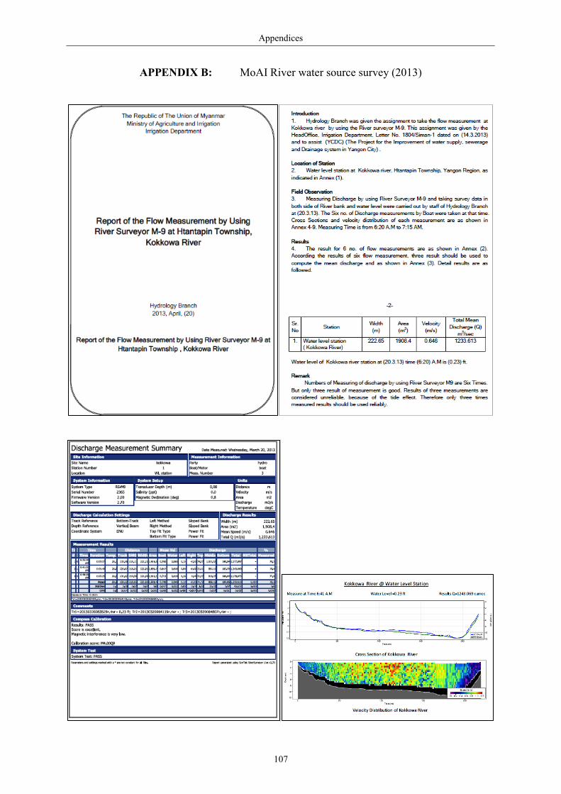
Appendices
107
APPENDIX B: MoAI River water source survey (2013)

Appendices
108

Appendices
109
APPENDIX C: DMH Climate data and Model Input data

Appendices
110

Appendices
111

Appendices
112
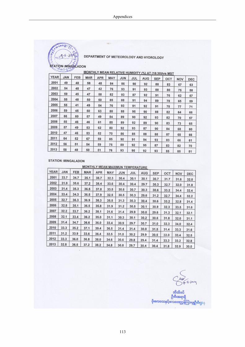
Appendices
113

Appendices
114

Appendices
115

Appendices
116
Table C1: Monthly variation demand in Yangon City (2007-2013)
Month Water consumption
units per connection
Monthly
variation (%) Month
Water consumption
units per connection
Monthly
variation (%)
Apr-07 44.5 9.0575 Oct-10 40.4 8.5892
May-07 42.2 8.5756 Nov-10 40.2 8.5532
Jun-07 43.2 8.7947 Dec-10 40 8.4949
Jul-07 41.1 8.3553 Jan-11 39 8.1451
Aug-07 40.9 8.3125 Feb-11 37.7 7.879
Sep-07 40.9 8.3149 Mar-11 37.4 7.826
Oct-07 41.5 8.4485 Apr-11 39.4 8.2304
Nov-07 40.3 8.2001 May-11 39.3 8.2112
Dec-07 41.7 8.4763 Jun-11 39.9 8.3297
Jan-08 41.1 8.5892 Jul-11 39.7 8.3048
Feb-08 37.7 7.8867 Aug-11 40.5 8.4719
Mar-08 37.3 7.8112 Sep-11 40.6 8.4779
Apr-08 42 8.7835 Oct-11 41.2 8.6135
May-08 39.3 8.227 Nov-11 42.2 8.829
Jun-08 39 8.1609 Dec-11 41.5 8.6815
Jul-08 41.2 8.6112 Jan-12 38.1 8.4648
Aug-08 41.2 8.6164 Feb-12 37.1 8.2386
Sep-08 40.7 8.5079 Mar-12 39.2 8.6992
Oct-08 39.7 8.2958 Apr-12 39.8 8.8296
Nov-08 40.4 8.4424 May-12 40 8.8943
Dec-08 38.6 8.0668 Jun-12 37.4 8.3157
Jan-09 35.5 8.1306 Jul-12 38 8.4399
Feb-09 34.9 7.9776 Aug-12 36.4 8.0927
Mar-09 34.3 7.8463 Sep-12 35.8 7.9591
Apr-09 37.3 8.5283 Oct-12 36.1 8.0102
May-09 37.5 8.5808 Nov-12 36 8.0005
Jun-09 37.1 8.4823 Dec-12 36.3 8.0555
Jul-09 36.4 8.3274 Jan-13 36.1 7.9481
Aug-09 36.1 8.2474 Feb-13 37.4 8.2521
Sep-09 36 8.2442 Mar-13 35.9 7.9021
Oct-09 36.5 8.3597 Apr-13 38.6 8.5013
Nov-09 37.8 8.6527 May-13 37.9 8.358
Dec-09 37.7 8.6226 Jun-13 37.6 8.2829
Jan-10 36.5 7.7515 Jul-13 37.2 8.1985
Feb-10 36.9 7.8411 Aug-13 36.7 8.0888
Mar-10 35.7 7.5865 Sep-13 38.2 8.4129
Apr-10 40.1 8.5196 Oct-13 38.2 8.4256
May-10 39.6 8.4073 Nov-13 39.2 8.6421
Jun-10 40.3 8.5623 Dec-13 40.8 8.9872
Jul-10 39.9 8.4762 Jan-14 38.8 7.8972
Aug-10 40.2 8.5483 Feb-14 38.4 7.8169
Sep-10 40.8 8.6702 Mar-14 38.1 7.7496

Appendices
117
Table C2: Monthly water charges income of EDWS, YCDC (2007-2013)
Month Domestic
connection
Income
(MMK)
Commercial
connection
Income
(MMK) Month
Domestic
connection
Income
(MMK)
Commercial
connection
Income
(MMK)
Apr-07 71381 89074979 8116 43423269 Oct-10 124555 131195765 10367 51730368
May-07 75598 94412200 8155 40645733 Nov-10 125281 130621121 10412 51839332
Jun-07 76126 92146291 8263 42998898 Dec-10 124485 130489818 10431 51411108
Jul-07 77546 89582445 8367 41403597 Jan-11 124666 126688194 10356 49897496
Aug-07 77848 85436021 8394 41943709 Feb-11 124814 124417410 10328 48018025
Sep-07 78900 86015082 8452 42335309 Mar-11 125381 125532395 10339 47602294
Oct-07 79237 88500815 8560 43421456 Apr-11 125147 128840403 10319 50175817
Nov-07 78053 89812495 8427 40764217 May-11 126309 128023606 10326 50294265
Dec-07 78595 88886117 8764 44468943 Jun-11 127024 131128728 10332 50954237
Jan-08 80410 86052738 8891 45034697 Jul-11 128636 133638054 10308 50552136
Feb-08 81923 82113927 8943 41522576 Aug-11 131798 137323901 10447 52475475
Mar-08 87402 90022859 9116 41466297 Sep-11 132699 141503997 10537 52613580
Apr-08 89850 97060885 9181 47687546 Oct-11 134510 146842847 10608 53651378
May-08 91470 90741385 9143 44873908 Nov-11 135748 149566812 10798 56173870
Jun-08 92527 100324596 9249 43749684 Dec-11 136590 150905749 10962 55790132
Jul-08 94824 101949414 9505 48232695 Jan-12 137665 146407398 12227 56491560
Aug-08 96015 104250531 9652 48872239 Feb-12 138895 143782917 12259 55202205
Sep-08 98376 104707539 9842 49342930 Mar-12 139670 148431071 12349 59075402
Oct-08 99460 104999921 9909 48251841 Apr-12 141773 224461151 12868 89969378
Nov-08 101687 106269973 10050 50172471 May-12 143197 227583920 13008 91683476
Dec-08 102103 105551940 10039 47500499 Jun-12 143779 224731587 12986 84511908
Jan-09 102429 98413326 10043 43876905 Jul-12 144902 223460311 13211 87947374
Feb-09 102562 96653898 10049 43126467 Aug-12 144782 215485810 13183 84113716
Mar-09 103285 98301032 10091 42282638 Sep-12 144801 214605197 13173 82410110
Apr-09 107945 116770350 10235 45722797 Oct-12 145376 215418416 13249 83559720
May-09 110987 120999214 10320 46345128 Nov-12 145701 216707478 13209 83089238
Jun-09 112099 118963537 10337 46154803 Dec-12 146652 219825623 13336 84421040
Jul-09 112936 114948553 10312 45594693 Jan-13 147510 221376830 13770 86513660
Aug-09 115163 117168012 10398 45420990 Feb-13 148287 215788176 13452 89363418
Sep-09 116042 117983199 10432 45556842 Mar-13 148717 215104381 13592 85694320
Oct-09 116717 117156806 10408 46450254 Apr-13 149238 229809904 13624 92452260
Nov-09 117110 116307820 10423 48728727 May-13 149714 229533964 13738 91377208
Dec-09 117237 115515741 10436 48692337 Jun-13 150725 235330936 14532 95056786
Jan-10 118094 114078920 10475 47190339 Jul-13 151719 240057066 15498 99663996
Feb-10 118629 114117267 10461 47865623 Aug-13 153037 248392928 16078 100813626
Mar-10 118907 114954099 10447 45804002 Sep-13 153398 255362616 16296 106603572
Apr-10 117640 125968836 10399 51111158 Oct-13 154473 262356068 16449 107120110
May-10 119363 127839550 10288 49724628 Nov-13 154960 267277471 16449 110131872
Jun-10 121620 134696554 10273 50281123 Dec-13 156439 272886034 16463 115495758
Jul-10 121831 135824692 10287 49601881 Jan-14 157382 274070046 16538 108977478
Aug-10 122871 134719562 10368 50802022 Feb-14 160788 278656076 16623 108267926
Sep-10 123805 136310662 10359 51607039 Mar-14 162184 280795316 16621 107081870

Appendices
118
Table C3: Effective precipitation (%) of Hmawbi station (1991-2013)
Month Eff Pcp Month Eff Pcp Month Eff Pcp Month Eff Pcp Month Eff Pcp Month Eff Pcp
Jan-91 100.00 Nov-94 100.00 Sep-98 85.85 Jul-02 19.12 May-06 80.21 Mar-10 100.00
Feb-91 100.00 Dec-94 100.00 Oct-98 75.23 Aug-02 13.97 Jun-06 38.83 Apr-10 100.00
Mar-91 100.00 Jan-95 100.00 Nov-98 100.00 Sep-02 14.72 Jul-06 14.57 May-10 61.51
Apr-91 100.00 Feb-95 100.00 Dec-98 100.00 Oct-02 100.00 Aug-06 16.49 Jun-10 21.22
May-91 100.00 Mar-95 100.00 Jan-99 100.00 Nov-02 54.75 Sep-06 26.00 Jul-10 35.68
Jun-91 18.52 Apr-95 100.00 Feb-99 100.00 Dec-02 100.00 Oct-06 79.25 Aug-10 21.52
Jul-91 14.49 May-95 57.02 Mar-99 100.00 Jan-03 100.00 Nov-06 100.00 Sep-10 39.39
Aug-91 13.89 Jun-95 15.12 Apr-99 91.43 Feb-03 100.00 Dec-06 100.00 Oct-10 44.00
Sep-91 32.83 Jul-95 18.17 May-99 24.99 Mar-03 100.00 Jan-07 100.00 Nov-10 100.00
Oct-91 76.29 Aug-95 26.61 Jun-99 19.16 Apr-03 100.00 Feb-07 100.00 Dec-10 100.00
Nov-91 81.15 Sep-95 18.46 Jul-99 11.97 May-03 58.76 Mar-07 100.00 Jan-11 100.00
Dec-91 100.00 Oct-95 87.28 Aug-99 16.17 Jun-03 13.49 Apr-07 100.00 Feb-11 100.00
Jan-92 100.00 Nov-95 100.00 Sep-99 26.67 Jul-03 24.67 May-07 14.82 Mar-11 100.00
Feb-92 100.00 Dec-95 100.00 Oct-99 49.57 Aug-03 19.34 Jun-07 17.94 Apr-11 100.00
Mar-92 100.00 Jan-96 100.00 Nov-99 100.00 Sep-03 25.84 Jul-07 15.73 May-11 38.97
Apr-92 100.00 Feb-96 100.00 Dec-99 100.00 Oct-03 100.00 Aug-07 21.72 Jun-11 10.53
May-92 76.62 Mar-96 100.00 Jan-00 100.00 Nov-03 100.00 Sep-07 13.50 Jul-11 18.79
Jun-92 19.22 Apr-96 100.00 Feb-00 100.00 Dec-03 100.00 Oct-07 35.03 Aug-11 23.01
Jul-92 13.48 May-96 30.31 Mar-00 100.00 Jan-04 100.00 Nov-07 100.00 Sep-11 17.55
Aug-92 14.08 Jun-96 19.28 Apr-00 100.00 Feb-04 100.00 Dec-07 100.00 Oct-11 85.64
Sep-92 24.43 Jul-96 22.64 May-00 28.75 Mar-04 100.00 Jan-08 100.00 Nov-11 100.00
Oct-92 42.90 Aug-96 18.73 Jun-00 16.47 Apr-04 100.00 Feb-08 100.00 Dec-11 100.00
Nov-92 100.00 Sep-96 23.42 Jul-00 16.51 May-04 27.02 Mar-08 100.00 Jan-12 100.00
Dec-92 100.00 Oct-96 45.58 Aug-00 24.19 Jun-04 11.36 Apr-08 100.00 Feb-12 100.00
Jan-93 100.00 Nov-96 70.07 Sep-00 32.43 Jul-04 23.76 May-08 17.21 Mar-12 100.00
Feb-93 100.00 Dec-96 100.00 Oct-00 97.43 Aug-04 12.33 Jun-08 26.23 Apr-12 100.00
Mar-93 100.00 Jan-97 100.00 Nov-00 100.00 Sep-04 23.62 Jul-08 13.50 May-12 100.00
Apr-93 100.00 Feb-97 100.00 Dec-00 100.00 Oct-04 100.00 Aug-08 20.16 Jun-12 17.56
May-93 52.92 Mar-97 100.00 Jan-01 100.00 Nov-04 100.00 Sep-08 27.88 Jul-12 11.84
Jun-93 21.46 Apr-97 100.00 Feb-01 100.00 Dec-04 100.00 Oct-08 74.90 Aug-12 10.74
Jul-93 21.84 May-97 95.28 Mar-01 100.00 Jan-05 100.00 Nov-08 100.00 Sep-12 19.71
Aug-93 9.20 Jun-97 21.83 Apr-01 100.00 Feb-05 100.00 Dec-08 100.00 Oct-12 100.00
Sep-93 21.88 Jul-97 12.06 May-01 53.48 Mar-05 100.00 Jan-09 100.00 Nov-12 77.34
Oct-93 100.00 Aug-97 12.37 Jun-01 13.91 Apr-05 100.00 Feb-09 100.00 Dec-12 100.00
Nov-93 100.00 Sep-97 22.85 Jul-01 14.86 May-05 100.00 Mar-09 100.00 Jan-13 100.00
Dec-93 100.00 Oct-97 51.85 Aug-01 21.36 Jun-05 22.30 Apr-09 100.00 Feb-13 100.00
Jan-94 100.00 Nov-97 100.00 Sep-01 41.55 Jul-05 14.11 May-09 46.22 Mar-13 100.00
Feb-94 100.00 Dec-97 100.00 Oct-01 35.79 Aug-05 15.50 Jun-09 18.01 Apr-13 100.00
Mar-94 100.00 Jan-98 100.00 Nov-01 100.00 Sep-05 22.70 Jul-09 12.35 May-13 66.19
Apr-94 100.00 Feb-98 100.00 Dec-01 100.00 Oct-05 60.81 Aug-09 25.81 Jun-13 16.74
May-94 87.15 Mar-98 100.00 Jan-02 100.00 Nov-05 100.00 Sep-09 21.58 Jul-13 13.87
Jun-94 14.09 Apr-98 100.00 Feb-02 100.00 Dec-05 100.00 Oct-09 83.33 Aug-13 11.11
Jul-94 13.02 May-98 65.74 Mar-02 100.00 Jan-06 100.00 Nov-09 100.00 Sep-13 13.88
Aug-94 11.59 Jun-98 18.81 Apr-02 100.00 Feb-06 100.00 Dec-09 100.00 Oct-13 41.01
Sep-94 25.19 Jul-98 27.90 May-02 54.77 Mar-06 100.00 Jan-10 100.00 Nov-13 100.00
Oct-94 100.00 Aug-98 16.15 Jun-02 14.23 Apr-06 100.00 Feb-10 100.00 Dec-13 100.00

Appendices
119
Table C4: Effective precipitation (%) of Mingalardon station (1991-2013)
Month Eff Pcp Month Eff Pcp Month Eff Pcp Month Eff Pcp Month Eff Pcp Month Eff Pcp
Jan-91 100.00 Nov-94 100.00 Sep-98 66.11 Jul-02 23.66 May-06 58.99 Mar-10 100.00
Feb-91 100.00 Dec-94 100.00 Oct-98 59.48 Aug-02 14.07 Jun-06 35.48 Apr-10 100.00
Mar-91 100.00 Jan-95 100.00 Nov-98 100.00 Sep-02 15.69 Jul-06 12.91 May-10 60.76
Apr-91 100.00 Feb-95 100.00 Dec-98 100.00 Oct-02 100.00 Aug-06 14.62 Jun-10 21.26
May-91 100.00 Mar-95 100.00 Jan-99 100.00 Nov-02 45.27 Sep-06 33.74 Jul-10 33.68
Jun-91 15.50 Apr-95 100.00 Feb-99 100.00 Dec-02 100.00 Oct-06 100.00 Aug-10 19.81
Jul-91 10.89 May-95 64.16 Mar-99 100.00 Jan-03 100.00 Nov-06 100.00 Sep-10 34.63
Aug-91 15.41 Jun-95 15.97 Apr-99 52.66 Feb-03 100.00 Dec-06 100.00 Oct-10 32.61
Sep-91 67.17 Jul-95 15.45 May-99 28.36 Mar-03 100.00 Jan-07 100.00 Nov-10 100.00
Oct-91 76.86 Aug-95 25.17 Jun-99 22.58 Apr-03 100.00 Feb-07 100.00 Dec-10 100.00
Nov-91 100.00 Sep-95 19.34 Jul-99 18.39 May-03 50.84 Mar-07 100.00 Jan-11 100.00
Dec-91 100.00 Oct-95 44.96 Aug-99 16.25 Jun-03 15.25 Apr-07 100.00 Feb-11 100.00
Jan-92 100.00 Nov-95 100.00 Sep-99 28.06 Jul-03 39.39 May-07 16.47 Mar-11 100.00
Feb-92 100.00 Dec-95 100.00 Oct-99 30.37 Aug-03 20.16 Jun-07 17.12 Apr-11 100.00
Mar-92 100.00 Jan-96 100.00 Nov-99 100.00 Sep-03 24.04 Jul-07 11.46 May-11 39.76
Apr-92 100.00 Feb-96 100.00 Dec-99 100.00 Oct-03 100.00 Aug-07 18.45 Jun-11 15.18
May-92 100.00 Mar-96 100.00 Jan-00 100.00 Nov-03 100.00 Sep-07 10.53 Jul-11 13.11
Jun-92 26.80 Apr-96 100.00 Feb-00 100.00 Dec-03 100.00 Oct-07 38.63 Aug-11 13.17
Jul-92 15.53 May-96 42.39 Mar-00 100.00 Jan-04 100.00 Nov-07 100.00 Sep-11 19.22
Aug-92 19.62 Jun-96 18.12 Apr-00 100.00 Feb-04 100.00 Dec-07 100.00 Oct-11 70.25
Sep-92 32.83 Jul-96 21.77 May-00 51.95 Mar-04 100.00 Jan-08 100.00 Nov-11 100.00
Oct-92 41.82 Aug-96 14.59 Jun-00 16.70 Apr-04 100.00 Feb-08 100.00 Dec-11 100.00
Nov-92 100.00 Sep-96 17.86 Jul-00 26.27 May-04 33.54 Mar-08 100.00 Jan-12 100.00
Dec-92 100.00 Oct-96 55.01 Aug-00 27.16 Jun-04 11.78 Apr-08 100.00 Feb-12 100.00
Jan-93 100.00 Nov-96 90.48 Sep-00 21.99 Jul-04 21.69 May-08 18.98 Mar-12 100.00
Feb-93 100.00 Dec-96 100.00 Oct-00 65.40 Aug-04 10.33 Jun-08 30.82 Apr-12 100.00
Mar-93 100.00 Jan-97 100.00 Nov-00 100.00 Sep-04 28.27 Jul-08 15.92 May-12 100.00
Apr-93 100.00 Feb-97 100.00 Dec-00 100.00 Oct-04 100.00 Aug-08 21.16 Jun-12 22.61
May-93 59.61 Mar-97 100.00 Jan-01 100.00 Nov-04 100.00 Sep-08 20.89 Jul-12 11.85
Jun-93 25.33 Apr-97 100.00 Feb-01 100.00 Dec-04 100.00 Oct-08 33.31 Aug-12 9.29
Jul-93 22.95 May-97 48.36 Mar-01 100.00 Jan-05 100.00 Nov-08 100.00 Sep-12 27.23
Aug-93 14.86 Jun-97 23.38 Apr-01 100.00 Feb-05 100.00 Dec-08 100.00 Oct-12 100.00
Sep-93 24.76 Jul-97 13.50 May-01 37.44 Mar-05 100.00 Jan-09 100.00 Nov-12 83.72
Oct-93 100.00 Aug-97 12.11 Jun-01 19.54 Apr-05 100.00 Feb-09 100.00 Dec-12 100.00
Nov-93 100.00 Sep-97 18.44 Jul-01 16.70 May-05 91.05 Mar-09 100.00 Jan-13 100.00
Dec-93 100.00 Oct-97 60.90 Aug-01 20.55 Jun-05 15.98 Apr-09 100.00 Feb-13 100.00
Jan-94 100.00 Nov-97 100.00 Sep-01 55.10 Jul-05 16.50 May-09 36.50 Mar-13 100.00
Feb-94 100.00 Dec-97 100.00 Oct-01 34.31 Aug-05 18.48 Jun-09 15.72 Apr-13 100.00
Mar-94 100.00 Jan-98 100.00 Nov-01 100.00 Sep-05 15.85 Jul-09 9.49 May-13 100.00
Apr-94 100.00 Feb-98 100.00 Dec-01 100.00 Oct-05 73.44 Aug-09 25.98 Jun-13 20.75
May-94 70.22 Mar-98 100.00 Jan-02 100.00 Nov-05 100.00 Sep-09 16.63 Jul-13 13.95
Jun-94 13.46 Apr-98 100.00 Feb-02 100.00 Dec-05 100.00 Oct-09 86.50 Aug-13 18.51
Jul-94 11.29 May-98 49.54 Mar-02 100.00 Jan-06 100.00 Nov-09 100.00 Sep-13 13.82
Aug-94 11.38 Jun-98 23.14 Apr-02 100.00 Feb-06 100.00 Dec-09 100.00 Oct-13 48.66
Sep-94 23.31 Jul-98 29.67 May-02 40.54 Mar-06 100.00 Jan-10 100.00 Nov-13 100.00
Oct-94 69.71 Aug-98 20.07 Jun-02 13.47 Apr-06 100.00 Feb-10 100.00 Dec-13 100.00

Appendices
120
Table C5: Reference Evapotranspiration ETo (mm) of Hmawbi station (1991-2013)
Month ETo Month ETo Month ETo Month ETo Month ETo Month ETo
Jan-91 111.29 Nov-94 111.30 Sep-98 105.60 Jul-02 97.34 May-06 128.34 Mar-10 137.95
Feb-91 117.60 Dec-94 110.05 Oct-98 112.84 Aug-02 80.91 Jun-06 96.30 Apr-10 176.10
Mar-91 155.00 Jan-95 109.43 Nov-98 104.40 Sep-02 87.90 Jul-06 89.90 May-10 155.62
Apr-91 157.20 Feb-95 115.36 Dec-98 104.16 Oct-02 118.42 Aug-06 85.56 Jun-10 92.10
May-91 135.47 Mar-95 145.70 Jan-99 102.92 Nov-02 109.50 Sep-06 107.10 Jul-10 99.20
Jun-91 91.50 Apr-95 164.40 Feb-99 108.92 Dec-02 102.30 Oct-06 112.53 Aug-10 85.87
Jul-91 88.66 May-95 145.39 Mar-99 152.83 Jan-03 99.20 Nov-06 106.20 Sep-10 90.60
Aug-91 75.02 Jun-95 91.50 Apr-99 134.40 Feb-03 111.72 Dec-06 98.27 Oct-10 100.75
Sep-91 90.60 Jul-95 91.76 May-99 117.18 Mar-03 151.28 Jan-07 97.96 Nov-10 112.20
Oct-91 107.57 Aug-95 86.49 Jun-99 88.50 Apr-03 179.10 Feb-07 105.56 Dec-10 97.65
Nov-91 112.80 Sep-95 98.40 Jul-99 84.63 May-03 146.32 Mar-07 152.21 Jan-11 96.10
Dec-91 105.09 Oct-95 113.46 Aug-99 85.56 Jun-03 98.10 Apr-07 176.70 Feb-11 106.40
Jan-92 109.12 Nov-95 105.90 Sep-99 93.60 Jul-03 95.48 May-07 108.50 Mar-11 130.20
Feb-92 122.67 Dec-95 110.67 Oct-99 100.13 Aug-03 93.62 Jun-07 89.70 Apr-11 144.30
Mar-92 155.62 Jan-96 110.36 Nov-99 102.60 Sep-03 100.50 Jul-07 84.94 May-11 110.67
Apr-92 158.70 Feb-96 118.03 Dec-99 104.16 Oct-03 116.87 Aug-07 81.22 Jun-11 83.10
May-92 147.87 Mar-96 157.79 Jan-00 122.14 Nov-03 95.10 Sep-07 77.10 Jul-11 92.07
Jun-92 96.30 Apr-96 153.60 Feb-00 114.26 Dec-03 105.71 Oct-07 94.24 Aug-11 82.15
Jul-92 90.21 May-96 122.14 Mar-00 149.42 Jan-04 105.71 Nov-07 109.20 Sep-11 79.50
Aug-92 83.08 Jun-96 98.70 Apr-00 144.90 Feb-04 112.81 Dec-07 93.31 Oct-11 101.06
Sep-92 88.20 Jul-96 98.27 May-00 130.51 Mar-04 159.96 Jan-08 98.27 Nov-11 112.50
Oct-92 101.68 Aug-96 89.90 Jun-00 90.90 Apr-04 173.10 Feb-08 106.72 Dec-11 103.85
Nov-92 108.30 Sep-96 99.30 Jul-00 90.83 May-04 142.91 Mar-08 145.70 Jan-12 108.19
Dec-92 110.67 Oct-96 107.57 Aug-00 88.04 Jun-04 90.30 Apr-08 149.70 Feb-12 118.03
Jan-93 106.64 Nov-96 104.40 Sep-00 88.20 Jul-04 96.72 May-08 99.82 Mar-12 145.70
Feb-93 117.60 Dec-96 104.47 Oct-00 102.30 Aug-04 81.53 Jun-08 87.60 Apr-12 163.50
Mar-93 157.79 Jan-97 106.64 Nov-00 111.90 Sep-04 97.80 Jul-08 85.56 May-12 124.62
Apr-93 165.00 Feb-97 117.04 Dec-00 107.26 Oct-04 105.71 Aug-08 91.14 Jun-12 86.40
May-93 144.46 Mar-97 153.45 Jan-01 100.13 Nov-04 116.70 Sep-08 90.90 Jul-12 81.22
Jun-93 101.10 Apr-97 162.00 Feb-01 113.40 Dec-04 101.99 Oct-08 102.61 Aug-12 79.98
Jul-93 99.82 May-97 155.31 Mar-01 156.24 Jan-05 110.36 Nov-08 103.80 Sep-12 94.80
Aug-93 80.60 Jun-97 100.20 Apr-01 177.90 Feb-05 122.08 Dec-08 102.30 Oct-12 114.39
Sep-93 89.70 Jul-97 84.63 May-01 134.23 Mar-05 159.65 Jan-09 105.09 Nov-12 99.00
Oct-93 129.89 Aug-97 89.90 Jun-01 94.20 Apr-05 186.60 Feb-09 105.00 Dec-12 99.20
Nov-93 117.60 Sep-97 82.50 Jul-01 89.59 May-05 148.49 Mar-09 140.12 Jan-13 98.58
Dec-93 107.88 Oct-97 115.63 Aug-01 88.66 Jun-05 84.30 Apr-09 150.90 Feb-13 111.44
Jan-94 110.36 Nov-97 103.20 Sep-01 104.70 Jul-05 89.90 May-09 128.96 Mar-13 147.56
Feb-94 117.04 Dec-97 107.26 Oct-01 101.99 Aug-05 84.94 Jun-09 84.30 Apr-13 177.30
Mar-94 145.70 Jan-98 108.50 Nov-01 89.40 Sep-05 91.50 Jul-09 82.15 May-13 146.94
Apr-94 164.40 Feb-98 113.96 Dec-01 95.17 Oct-05 110.67 Aug-09 95.48 Jun-13 90.90
May-94 124.62 Mar-98 158.41 Jan-02 100.13 Nov-05 98.10 Sep-09 86.10 Jul-13 81.84
Jun-94 88.50 Apr-98 152.70 Feb-02 113.12 Dec-05 103.54 Oct-09 104.16 Aug-13 84.32
Jul-94 87.73 May-98 147.25 Mar-02 153.14 Jan-06 103.85 Nov-09 112.20 Sep-13 83.70
Aug-94 79.05 Jun-98 96.30 Apr-02 181.80 Feb-06 115.92 Dec-09 100.44 Oct-13 104.16
Sep-94 92.70 Jul-98 94.86 May-02 138.57 Mar-06 153.76 Jan-10 99.20 Nov-13 105.00
Oct-94 119.35 Aug-98 92.38 Jun-02 83.70 Apr-06 174.90 Feb-10 110.32 Dec-13 96.10

Appendices
121
Table C6: Reference Evapotranspiration ETo (mm) of Mingalardon station (1991-2013)
Month ETo Month ETo Month ETo Month ETo Month ETo Month ETo
Jan-91 126.17 Nov-94 120.30 Sep-98 107.10 Jul-02 98.89 May-06 139.81 Mar-10 141.67
Feb-91 128.24 Dec-94 120.90 Oct-98 117.18 Aug-02 82.15 Jun-06 102.90 Apr-10 171.30
Mar-91 159.96 Jan-95 124.31 Nov-98 114.00 Sep-02 88.50 Jul-06 91.76 May-10 182.28
Apr-91 171.00 Feb-95 126.28 Dec-98 115.01 Oct-02 128.03 Aug-06 90.21 Jun-10 92.70
May-91 165.23 Mar-95 150.66 Jan-99 117.80 Nov-02 123.60 Sep-06 111.00 Jul-10 105.09
Jun-91 93.60 Apr-95 178.80 Feb-99 119.84 Dec-02 124.31 Oct-06 128.96 Aug-10 88.35
Jul-91 90.83 May-95 147.56 Mar-99 157.79 Jan-03 128.65 Nov-06 143.70 Sep-10 94.20
Aug-91 77.19 Jun-95 93.60 Apr-99 146.40 Feb-03 152.60 Dec-06 132.68 Oct-10 100.44
Sep-91 92.70 Jul-95 93.93 May-99 119.97 Mar-03 185.69 Jan-07 121.21 Nov-10 131.40
Oct-91 112.22 Aug-95 88.35 Jun-99 90.30 Apr-03 202.50 Feb-07 127.96 Dec-10 117.49
Nov-91 122.10 Sep-95 100.20 Jul-99 86.80 May-03 170.81 Mar-07 168.02 Jan-11 119.66
Dec-91 115.94 Oct-95 117.80 Aug-99 87.42 Jun-03 99.30 Apr-07 200.70 Feb-11 115.08
Jan-92 123.69 Nov-95 115.50 Sep-99 95.70 Jul-03 100.44 May-07 115.63 Mar-11 126.17
Feb-92 133.98 Dec-95 121.21 Oct-99 105.09 Aug-03 93.93 Jun-07 92.10 Apr-11 166.50
Mar-92 160.58 Jan-96 125.24 Nov-99 112.20 Sep-03 99.30 Jul-07 87.11 May-11 112.53
Apr-92 172.50 Feb-96 129.34 Dec-99 115.01 Oct-03 129.89 Aug-07 83.39 Jun-11 89.10
May-92 149.73 Mar-96 162.75 Jan-00 136.40 Nov-03 128.70 Sep-07 77.40 Jul-11 94.24
Jun-92 98.10 Apr-96 167.10 Feb-00 125.57 Dec-03 136.09 Oct-07 100.44 Aug-11 83.39
Jul-92 92.38 May-96 124.62 Mar-00 154.38 Jan-04 138.88 Nov-07 125.70 Sep-11 81.30
Aug-92 84.94 Jun-96 100.20 Apr-00 157.80 Feb-04 140.36 Dec-07 125.24 Oct-11 108.19
Sep-92 90.60 Jul-96 100.13 May-00 132.99 Mar-04 186.31 Jan-08 126.48 Nov-11 132.60
Oct-92 106.64 Aug-96 91.45 Jun-00 92.70 Apr-04 205.50 Feb-08 141.52 Dec-11 129.89
Nov-92 117.60 Sep-96 101.10 Jul-00 93.00 May-04 143.53 Mar-08 177.32 Jan-12 132.37
Dec-92 121.21 Oct-96 112.22 Aug-00 89.90 Jun-04 95.10 Apr-08 155.70 Feb-12 143.55
Jan-93 121.52 Nov-96 114.00 Sep-00 90.60 Jul-04 96.10 May-08 110.67 Mar-12 171.12
Feb-93 128.24 Dec-96 115.32 Oct-00 107.26 Aug-04 79.36 Jun-08 90.60 Apr-12 189.30
Mar-93 162.75 Jan-97 121.52 Nov-00 120.90 Sep-04 97.80 Jul-08 88.66 May-12 140.43
Apr-93 179.40 Feb-97 127.96 Dec-00 118.11 Oct-04 118.11 Aug-08 93.31 Jun-12 90.90
May-93 146.63 Mar-97 158.41 Jan-01 148.80 Nov-04 144.60 Sep-08 87.30 Jul-12 82.15
Jun-93 102.60 Apr-97 176.40 Feb-01 142.52 Dec-04 127.10 Oct-08 102.92 Aug-12 76.57
Jul-93 101.68 May-97 157.17 Mar-01 185.69 Jan-05 133.61 Nov-08 120.30 Sep-12 97.50
Aug-93 82.77 Jun-97 101.70 Apr-01 223.20 Feb-05 145.88 Dec-08 119.04 Oct-12 121.52
Sep-93 92.10 Jul-97 86.80 May-01 142.29 Mar-05 183.21 Jan-09 117.18 Nov-12 108.00
Oct-93 133.30 Aug-97 91.45 Jun-01 101.40 Apr-05 205.80 Feb-09 150.36 Dec-12 117.80
Nov-93 126.60 Sep-97 85.20 Jul-01 90.83 May-05 159.34 Mar-09 169.88 Jan-13 127.72
Dec-93 118.42 Oct-97 119.97 Aug-01 88.35 Jun-05 85.20 Apr-09 176.10 Feb-13 143.36
Jan-94 125.24 Nov-97 112.80 Sep-01 108.00 Jul-05 89.90 May-09 125.55 Mar-13 180.42
Feb-94 127.96 Dec-97 118.11 Oct-01 109.12 Aug-05 87.42 Jun-09 87.90 Apr-13 206.40
Mar-94 150.66 Jan-98 123.38 Nov-01 120.60 Sep-05 95.10 Jul-09 81.53 May-13 152.21
Apr-94 178.80 Feb-98 124.88 Dec-01 127.41 Oct-05 123.38 Aug-09 99.51 Jun-13 91.50
May-94 127.10 Mar-98 163.37 Jan-02 133.92 Nov-05 114.60 Sep-09 87.00 Jul-13 82.46
Jun-94 90.30 Apr-98 166.50 Feb-02 144.20 Dec-05 124.93 Oct-09 107.26 Aug-13 87.73
Jul-94 89.90 May-98 149.11 Mar-02 195.30 Jan-06 138.26 Nov-09 133.20 Sep-13 84.00
Aug-94 81.22 Jun-98 98.10 Apr-02 200.40 Feb-06 155.12 Dec-09 128.65 Oct-13 111.91
Sep-94 95.10 Jul-98 97.03 May-02 158.10 Mar-06 182.59 Jan-10 127.41 Nov-13 115.80
Oct-94 123.38 Aug-98 93.93 Jun-02 83.10 Apr-06 194.10 Feb-10 120.12 Dec-13 105.09

Appendices
122
Table C7: Precipitation (mm) of Hmawbi station (1991-2013)
Month Pcp Month Pcp Month Pcp Month Pcp Month Pcp Month Pcp
Jan-91 0 Nov-94 83 Sep-98 123 Jul-02 509 May-06 160 Mar-10 0
Feb-91 0 Dec-94 3 Oct-98 150 Aug-02 579 Jun-06 248 Apr-10 0
Mar-91 6 Jan-95 0 Nov-98 83 Sep-02 597 Jul-06 617 May-10 253
Apr-91 7 Feb-95 0 Dec-98 0 Oct-02 93 Aug-06 519 Jun-10 434
May-91 26 Mar-95 0 Jan-99 0 Nov-02 200 Sep-06 412 Jul-10 278
Jun-91 494 Apr-95 0 Feb-99 6 Dec-02 18 Oct-06 122 Aug-10 399
Jul-91 612 May-95 255 Mar-99 18 Jan-03 6 Nov-06 0 Sep-10 231
Aug-91 540 Jun-95 605 Apr-99 147 Feb-03 0 Dec-06 0 Oct-10 229
Sep-91 276 Jul-95 505 May-99 469 Mar-03 1 Jan-07 0 Nov-10 0
Oct-91 141 Aug-95 325 Jun-99 462 Apr-03 3 Feb-07 0 Dec-10 61
Nov-91 139 Sep-95 533 Jul-99 707 May-03 249 Mar-07 0 Jan-11 81
Dec-91 20 Oct-95 130 Aug-99 529 Jun-03 727 Apr-07 2 Feb-11 0
Jan-92 0 Nov-95 99 Sep-99 351 Jul-03 387 May-07 732 Mar-11 108
Feb-92 6 Dec-95 0 Oct-99 202 Aug-03 484 Jun-07 500 Apr-11 0
Mar-92 0 Jan-96 0 Nov-99 48 Sep-03 389 Jul-07 540 May-11 284
Apr-92 10 Feb-96 68 Dec-99 0 Oct-03 66 Aug-07 374 Jun-11 789
May-92 193 Mar-96 7 Jan-00 0 Nov-03 2 Sep-07 571 Jul-11 490
Jun-92 501 Apr-96 31 Feb-00 1 Dec-03 0 Oct-07 269 Aug-11 357
Jul-92 669 May-96 403 Mar-00 34 Jan-04 7 Nov-07 23 Sep-11 453
Aug-92 590 Jun-96 512 Apr-00 15 Feb-04 0 Dec-07 0 Oct-11 118
Sep-92 361 Jul-96 434 May-00 454 Mar-04 0 Jan-08 16 Nov-11 0
Oct-92 237 Aug-96 480 Jun-00 552 Apr-04 0 Feb-08 28 Dec-11 0
Nov-92 33 Sep-96 424 Jul-00 550 May-04 529 Mar-08 0 Jan-12 0
Dec-92 0 Oct-96 236 Aug-00 364 Jun-04 795 Apr-08 148 Feb-12 0
Jan-93 0 Nov-96 149 Sep-00 272 Jul-04 407 May-08 580 Mar-12 0
Feb-93 0 Dec-96 0 Oct-00 105 Aug-04 661 Jun-08 334 Apr-12 18
Mar-93 0 Jan-97 0 Nov-00 1 Sep-04 414 Jul-08 634 May-12 113
Apr-93 7 Feb-97 0 Dec-00 0 Oct-04 87 Aug-08 453 Jun-12 492
May-93 273 Mar-97 5 Jan-01 1 Nov-04 0 Sep-08 326 Jul-12 686
Jun-93 471 Apr-97 41 Feb-01 1 Dec-04 0 Oct-08 137 Aug-12 745
Jul-93 457 May-97 163 Mar-01 21 Jan-05 0 Nov-08 12 Sep-12 481
Aug-93 876 Jun-97 459 Apr-01 0 Feb-05 0 Dec-08 0 Oct-12 73
Sep-93 410 Jul-97 702 May-01 251 Mar-05 0 Jan-09 0 Nov-12 128
Oct-93 83 Aug-97 727 Jun-01 677 Apr-05 0 Feb-09 0 Dec-12 2
Nov-93 0 Sep-97 361 Jul-01 603 May-05 76 Mar-09 0 Jan-13 0
Dec-93 0 Oct-97 223 Aug-01 415 Jun-05 378 Apr-09 104 Feb-13 1
Jan-94 0 Nov-97 20 Sep-01 252 Jul-05 637 May-09 279 Mar-13 0
Feb-94 0 Dec-97 0 Oct-01 285 Aug-05 548 Jun-09 468 Apr-13 0
Mar-94 107 Jan-98 0 Nov-01 20 Sep-05 403 Jul-09 665 May-13 222
Apr-94 0 Feb-98 0 Dec-01 0 Oct-05 182 Aug-09 385 Jun-13 543
May-94 143 Mar-98 0 Jan-02 0 Nov-05 67 Sep-09 399 Jul-13 590
Jun-94 628 Apr-98 10 Feb-02 0 Dec-05 50 Oct-09 125 Aug-13 759
Jul-94 674 May-98 224 Mar-02 0 Jan-06 0 Nov-09 0 Sep-13 603
Aug-94 682 Jun-98 512 Apr-02 0 Feb-06 0 Dec-09 0 Oct-13 254
Sep-94 368 Jul-98 340 May-02 253 Mar-06 0 Jan-10 8 Nov-13 25
Oct-94 34 Aug-98 572 Jun-02 588 Apr-06 152 Feb-10 0 Dec-13 0

Appendices
123
Table C8: Precipitation (mm) of Mingalardon station (1991-2013)
Month Pcp Month Pcp Month Pcp Month Pcp Month Pcp Month Pcp
Jan-91 0 Nov-94 27 Sep-98 162 Jul-02 418 May-06 237 Mar-10 0
Feb-91 0 Dec-94 0 Oct-98 197 Aug-02 584 Jun-06 290 Apr-10 0
Mar-91 0 Jan-95 0 Nov-98 11 Sep-02 564 Jul-06 711 May-10 300
Apr-91 17 Feb-95 0 Dec-98 0 Oct-02 111 Aug-06 617 Jun-10 436
May-91 42 Mar-95 0 Jan-99 0 Nov-02 273 Sep-06 329 Jul-10 312
Jun-91 604 Apr-95 0 Feb-99 0 Dec-02 0 Oct-06 128 Aug-10 446
Jul-91 834 May-95 230 Mar-99 35 Jan-03 3 Nov-06 0 Sep-10 268
Aug-91 501 Jun-95 586 Apr-99 278 Feb-03 0 Dec-06 0 Oct-10 308
Sep-91 138 Jul-95 608 May-99 423 Mar-03 3 Jan-07 0 Nov-10 14
Oct-91 146 Aug-95 351 Jun-99 400 Apr-03 0 Feb-07 0 Dec-10 11
Nov-91 21 Sep-95 518 Jul-99 472 May-03 336 Mar-07 0 Jan-11 50
Dec-91 19 Oct-95 262 Aug-99 538 Jun-03 651 Apr-07 0 Feb-11 0
Jan-92 0 Nov-95 88 Sep-99 341 Jul-03 255 May-07 702 Mar-11 97
Feb-92 0 Dec-95 0 Oct-99 346 Aug-03 466 Jun-07 538 Apr-11 8
Mar-92 0 Jan-96 0 Nov-99 65 Sep-03 413 Jul-07 760 May-11 283
Apr-92 2 Feb-96 59 Dec-99 0 Oct-03 59 Aug-07 452 Jun-11 587
May-92 129 Mar-96 4 Jan-00 0 Nov-03 5 Sep-07 735 Jul-11 719
Jun-92 366 Apr-96 45 Feb-00 0 Dec-03 0 Oct-07 260 Aug-11 633
Jul-92 595 May-96 294 Mar-00 0 Jan-04 3 Nov-07 3 Sep-11 423
Aug-92 433 Jun-96 553 Apr-00 99 Feb-04 0 Dec-07 0 Oct-11 154
Sep-92 276 Jul-96 460 May-00 256 Mar-04 0 Jan-08 4 Nov-11 0
Oct-92 255 Aug-96 627 Jun-00 555 Apr-04 2 Feb-08 13 Dec-11 0
Nov-92 14 Sep-96 566 Jul-00 354 May-04 428 Mar-08 17 Jan-12 0
Dec-92 2 Oct-96 204 Aug-00 331 Jun-04 807 Apr-08 121 Feb-12 0
Jan-93 0 Nov-96 126 Sep-00 412 Jul-04 443 May-08 583 Mar-12 13
Feb-93 0 Dec-96 7 Oct-00 164 Aug-04 768 Jun-08 294 Apr-12 5
Mar-93 0 Jan-97 0 Nov-00 2 Sep-04 346 Jul-08 557 May-12 119
Apr-93 0 Feb-97 0 Dec-00 0 Oct-04 49 Aug-08 441 Jun-12 402
May-93 246 Mar-97 0 Jan-01 0 Nov-04 1 Sep-08 418 Jul-12 693
Jun-93 405 Apr-97 37 Feb-01 0 Dec-04 0 Oct-08 309 Aug-12 824
Jul-93 443 May-97 325 Mar-01 36 Jan-05 55 Nov-08 45 Sep-12 358
Aug-93 557 Jun-97 435 Apr-01 0 Feb-05 0 Dec-08 0 Oct-12 96
Sep-93 372 Jul-97 643 May-01 380 Mar-05 15 Jan-09 0 Nov-12 129
Oct-93 106 Aug-97 755 Jun-01 519 Apr-05 22 Feb-09 0 Dec-12 5
Nov-93 18 Sep-97 462 Jul-01 544 May-05 175 Mar-09 0 Jan-13 3
Dec-93 0 Oct-97 197 Aug-01 430 Jun-05 533 Apr-09 29 Feb-13 0
Jan-94 0 Nov-97 51 Sep-01 196 Jul-05 545 May-09 344 Mar-13 0
Feb-94 0 Dec-97 0 Oct-01 318 Aug-05 473 Jun-09 559 Apr-13 0
Mar-94 114 Jan-98 0 Nov-01 34 Sep-05 600 Jul-09 859 May-13 120
Apr-94 0 Feb-98 0 Dec-01 7 Oct-05 168 Aug-09 383 Jun-13 441
May-94 181 Mar-98 0 Jan-02 0 Nov-05 61 Sep-09 523 Jul-13 591
Jun-94 671 Apr-98 11 Feb-02 0 Dec-05 0 Oct-09 124 Aug-13 474
Jul-94 796 May-98 301 Mar-02 0 Jan-06 0 Nov-09 16 Sep-13 608
Aug-94 714 Jun-98 424 Apr-02 4 Feb-06 0 Dec-09 0 Oct-13 230
Sep-94 408 Jul-98 327 May-02 390 Mar-06 0 Jan-10 0 Nov-13 64
Oct-94 177 Aug-98 468 Jun-02 617 Apr-06 149 Feb-10 0 Dec-13 0

Appendices
124
Table C9: Precipitation (mm) of Kaba-aye station (1991-2013)
Month Eff Pcp Month Eff Pcp Month Eff Pcp Month Eff Pcp Month Eff Pcp Month Eff Pcp
Jan-91 126.17 Nov-94 120.30 Sep-98 107.10 Jul-02 98.89 May-06 139.81 Mar-10 141.67
Feb-91 128.24 Dec-94 120.90 Oct-98 117.18 Aug-02 82.15 Jun-06 102.90 Apr-10 171.30
Mar-91 159.96 Jan-95 124.31 Nov-98 114.00 Sep-02 88.50 Jul-06 91.76 May-10 182.28
Apr-91 171.00 Feb-95 126.28 Dec-98 115.01 Oct-02 128.03 Aug-06 90.21 Jun-10 92.70
May-91 165.23 Mar-95 150.66 Jan-99 117.80 Nov-02 123.60 Sep-06 111.00 Jul-10 105.09
Jun-91 93.60 Apr-95 178.80 Feb-99 119.84 Dec-02 124.31 Oct-06 128.96 Aug-10 88.35
Jul-91 90.83 May-95 147.56 Mar-99 157.79 Jan-03 128.65 Nov-06 143.70 Sep-10 94.20
Aug-91 77.19 Jun-95 93.60 Apr-99 146.40 Feb-03 152.60 Dec-06 132.68 Oct-10 100.44
Sep-91 92.70 Jul-95 93.93 May-99 119.97 Mar-03 185.69 Jan-07 121.21 Nov-10 131.40
Oct-91 112.22 Aug-95 88.35 Jun-99 90.30 Apr-03 202.50 Feb-07 127.96 Dec-10 117.49
Nov-91 122.10 Sep-95 100.20 Jul-99 86.80 May-03 170.81 Mar-07 168.02 Jan-11 119.66
Dec-91 115.94 Oct-95 117.80 Aug-99 87.42 Jun-03 99.30 Apr-07 200.70 Feb-11 115.08
Jan-92 123.69 Nov-95 115.50 Sep-99 95.70 Jul-03 100.44 May-07 115.63 Mar-11 126.17
Feb-92 133.98 Dec-95 121.21 Oct-99 105.09 Aug-03 93.93 Jun-07 92.10 Apr-11 166.50
Mar-92 160.58 Jan-96 125.24 Nov-99 112.20 Sep-03 99.30 Jul-07 87.11 May-11 112.53
Apr-92 172.50 Feb-96 129.34 Dec-99 115.01 Oct-03 129.89 Aug-07 83.39 Jun-11 89.10
May-92 149.73 Mar-96 162.75 Jan-00 136.40 Nov-03 128.70 Sep-07 77.40 Jul-11 94.24
Jun-92 98.10 Apr-96 167.10 Feb-00 125.57 Dec-03 136.09 Oct-07 100.44 Aug-11 83.39
Jul-92 92.38 May-96 124.62 Mar-00 154.38 Jan-04 138.88 Nov-07 125.70 Sep-11 81.30
Aug-92 84.94 Jun-96 100.20 Apr-00 157.80 Feb-04 140.36 Dec-07 125.24 Oct-11 108.19
Sep-92 90.60 Jul-96 100.13 May-00 132.99 Mar-04 186.31 Jan-08 126.48 Nov-11 132.60
Oct-92 106.64 Aug-96 91.45 Jun-00 92.70 Apr-04 205.50 Feb-08 141.52 Dec-11 129.89
Nov-92 117.60 Sep-96 101.10 Jul-00 93.00 May-04 143.53 Mar-08 177.32 Jan-12 132.37
Dec-92 121.21 Oct-96 112.22 Aug-00 89.90 Jun-04 95.10 Apr-08 155.70 Feb-12 143.55
Jan-93 121.52 Nov-96 114.00 Sep-00 90.60 Jul-04 96.10 May-08 110.67 Mar-12 171.12
Feb-93 128.24 Dec-96 115.32 Oct-00 107.26 Aug-04 79.36 Jun-08 90.60 Apr-12 189.30
Mar-93 162.75 Jan-97 121.52 Nov-00 120.90 Sep-04 97.80 Jul-08 88.66 May-12 140.43
Apr-93 179.40 Feb-97 127.96 Dec-00 118.11 Oct-04 118.11 Aug-08 93.31 Jun-12 90.90
May-93 146.63 Mar-97 158.41 Jan-01 148.80 Nov-04 144.60 Sep-08 87.30 Jul-12 82.15
Jun-93 102.60 Apr-97 176.40 Feb-01 142.52 Dec-04 127.10 Oct-08 102.92 Aug-12 76.57
Jul-93 101.68 May-97 157.17 Mar-01 185.69 Jan-05 133.61 Nov-08 120.30 Sep-12 97.50
Aug-93 82.77 Jun-97 101.70 Apr-01 223.20 Feb-05 145.88 Dec-08 119.04 Oct-12 121.52
Sep-93 92.10 Jul-97 86.80 May-01 142.29 Mar-05 183.21 Jan-09 117.18 Nov-12 108.00
Oct-93 133.30 Aug-97 91.45 Jun-01 101.40 Apr-05 205.80 Feb-09 150.36 Dec-12 117.80
Nov-93 126.60 Sep-97 85.20 Jul-01 90.83 May-05 159.34 Mar-09 169.88 Jan-13 127.72
Dec-93 118.42 Oct-97 119.97 Aug-01 88.35 Jun-05 85.20 Apr-09 176.10 Feb-13 143.36
Jan-94 125.24 Nov-97 112.80 Sep-01 108.00 Jul-05 89.90 May-09 125.55 Mar-13 180.42
Feb-94 127.96 Dec-97 118.11 Oct-01 109.12 Aug-05 87.42 Jun-09 87.90 Apr-13 206.40
Mar-94 150.66 Jan-98 123.38 Nov-01 120.60 Sep-05 95.10 Jul-09 81.53 May-13 152.21
Apr-94 178.80 Feb-98 124.88 Dec-01 127.41 Oct-05 123.38 Aug-09 99.51 Jun-13 91.50
May-94 127.10 Mar-98 163.37 Jan-02 133.92 Nov-05 114.60 Sep-09 87.00 Jul-13 82.46
Jun-94 90.30 Apr-98 166.50 Feb-02 144.20 Dec-05 124.93 Oct-09 107.26 Aug-13 87.73
Jul-94 89.90 May-98 149.11 Mar-02 195.30 Jan-06 138.26 Nov-09 133.20 Sep-13 84.00
Aug-94 81.22 Jun-98 98.10 Apr-02 200.40 Feb-06 155.12 Dec-09 128.65 Oct-13 111.91
Sep-94 95.10 Jul-98 97.03 May-02 158.10 Mar-06 182.59 Jan-10 127.41 Nov-13 115.80
Oct-94 123.38 Aug-98 93.93 Jun-02 83.10 Apr-06 194.10 Feb-10 120.12 Dec-13 105.09

Appendices
125
Table C10: Net Evaporation (mm) of Hmawbi station (1991-2013)
Month Net Eva Month Net Eva Month Net Eva Month Net Eva Month Net Eva Month Net Eva
Jan-91 108.4 Nov-94 46.8 Sep-98 -19 02-Jul -434.6 06-May -45.3 10-Mar 167.4
Feb-91 160.1 Dec-94 110.6 Oct-98 -32.3 02-Aug -504.6 06-Jun -182 10-Apr 177
Mar-91 184.9 Jan-95 126 Nov-98 36.2 02-Sep -522 06-Jul -545.7 10-May -88.7
Apr-91 141.6 Feb-95 117.5 Dec-98 127.1 02-Oct 0 06-Aug -447.7 10-Jun -359
May-91 125.1 Mar-95 161.2 Jan-99 136.4 02-Nov -107 06-Sep -337 10-Jul -206.7
Jun-91 -446.7 Apr-95 198.5 Feb-99 128.2 02-Dec 65.7 06-Oct -25.9 10-Aug -330.8
Jul-91 -573.6 May-95 -120.3 Mar-99 184.9 03-Jan 80.8 06-Nov 120 10-Sep -162
Aug-91 -507.4 Jun-95 -537.1 Apr-99 -0.3 03-Feb 109.2 06-Dec 127.1 10-Oct -145.3
Sep-91 -206 Jul-95 -406.8 May-99 -341.4 03-Mar 154 07-Jan 86.8 10-Nov 114
Oct-91 -35.2 Aug-95 -251.6 Jun-99 -371.9 03-Apr 174 07-Feb 117.6 10-Dec 44.4
Nov-91 -28 Sep-95 -460.5 Jul-99 -621.2 03-May -125 07-Mar 151.9 11-Jan 15.1
Dec-91 103.5 Oct-95 -18.5 Aug-99 -439.3 03-Jun -643 07-Apr 154 11-Feb 114.8
Jan-92 104.9 Nov-95 19 Sep-99 -248 03-Jul -294 07-May -617.3 11-Mar 12.9
Feb-92 97 Dec-95 115.1 Oct-99 -83.8 03-Aug -418.9 07-Jun -434 11-Apr 165
Mar-92 150 Jan-96 117 Nov-99 91.2 03-Sep -311 07-Jul -468.7 11-May -181.7
Apr-92 161.7 Feb-96 73.4 Dec-99 150.2 03-Oct 42.5 07-Aug -302.7 11-Jun -720
May-92 -52.5 Mar-96 155 Jan-00 140.4 03-Nov 112 07-Sep -496 11-Jul -418.7
Jun-92 -442.8 Apr-96 128.1 Feb-00 149.8 03-Dec 102.3 07-Oct -172.9 11-Aug -282.6
Jul-92 -615.9 May-96 -270.5 Mar-00 160.8 04-Jan 73.6 07-Nov 97 11-Sep -369
Aug-92 -539.5 Jun-96 -445.2 Apr-00 167.6 04-Feb 92.8 07-Dec 127.1 11-Oct -3.3
Sep-92 -304.2 Jul-96 -351.8 May-00 -340.6 04-Mar 155 08-Jan 89.4 11-Nov 141
Oct-92 -153.4 Aug-96 -408.4 Jun-00 -444 04-Apr 177 08-Feb 96.7 11-Dec 120.9
Nov-92 78.5 Sep-96 -332.5 Jul-00 -454.1 04-May -411.2 08-Mar 151.9 12-Jan 114.7
Dec-92 104.1 Oct-96 -119.2 Aug-00 -255.3 04-Jun -696 08-Apr -4 12-Feb 145
Jan-93 126.3 Nov-96 -35.2 Sep-00 -179.2 04-Jul -345 08-May -505.6 12-Mar 179.8
Feb-93 115.7 Dec-96 129.2 Oct-00 5.2 04-Aug -614.5 08-Jun -265 12-Apr 171
Mar-93 149 Jan-97 115.5 Nov-00 122.6 04-Sep -348 08-Jul -575.1 12-May 32.7
Apr-93 165.5 Feb-97 129.4 Dec-00 136 04-Oct -0.2 08-Aug -391 12-Jun -429
May-93 -146.9 Mar-97 147.8 01-Jan 144.7 04-Nov 99 08-Sep -254 12-Jul -620.9
Jun-93 -387.6 Apr-97 107.6 01-Feb 161.4 04-Dec 93 08-Oct -50.2 12-Aug -670.6
Jul-93 -376 May-97 -30.5 01-Mar 149.5 05-Jan 99.2 08-Nov 96 12-Sep -376
Aug-93 -785.6 Jun-97 -386 01-Apr 240 05-Feb 117.6 08-Dec 114.7 12-Oct 63.4
Sep-93 -315.5 Jul-97 -647.1 01-May -120.8 05-Mar 155 09-Jan 124 12-Nov -8
Oct-93 29.4 Aug-97 -677.5 01-Jun -587 05-Apr 162 09-Feb 120.4 12-Dec 112.7
Nov-93 141.3 Sep-97 -307.8 01-Jul -519.3 05-May 41.8 09-Mar 158.1 13-Jan 133.3
Dec-93 122.2 Oct-97 -134.4 01-Aug -322 05-Jun -306 09-Apr 22 13-Feb 164.2
Jan-94 114.9 Nov-97 73.5 01-Sep -138 05-Jul -553.3 09-May -167.4 13-Mar 189.1
Feb-94 130 Dec-97 121.8 01-Oct -161 05-Aug -464.3 09-Jun -411 13-Apr 207
Mar-94 34.7 Jan-98 137.1 01-Nov 115 05-Sep -322 09-Jul -606.1 13-May -82.5
Apr-94 158.7 Feb-98 123.9 01-Dec 130.2 05-Oct -70.4 09-Aug -323 13-Jun -486
May-94 -28.8 Mar-98 200.2 02-Jan 86.8 05-Nov 29 09-Sep -312 13-Jul -546.6
Jun-94 -563.7 Apr-98 228.1 02-Feb 128.8 05-Dec 39.9 09-Oct -25.8 13-Aug -697
Jul-94 -602.1 May-98 -30.6 02-Mar 164.3 06-Jan 86.8 09-Nov 120 13-Sep -543
Aug-94 -625.3 Jun-98 -425.4 02-Apr 168 06-Feb 117.6 09-Dec 99.2 13-Oct -148.6
Sep-94 -291.4 Jul-98 -269.9 02-May -119.7 06-Mar 151.9 10-Jan 91.2 13-Nov 101
Oct-94 72.8 Aug-98 -507.1 02-Jun -501 06-Apr 4 10-Feb 126 13-Dec 83.7

Appendices
126
Table C11: Net Evaporation (mm) of Mingalardon station (1991-2013)
Month Net Eva Month Net Eva Month Net Eva Month Net Eva Month Net Eva Month Net Eva
Jan-91 108.4 Nov-94 102.8 Sep-98 -58 02-Jul -343.6 06-May -122.3 10-Mar 167.4
Feb-91 160.1 Dec-94 113.6 Oct-98 -79.3 02-Aug -509.6 06-Jun -224 10-Apr 177
Mar-91 190.9 Jan-95 126 Nov-98 108.2 02-Sep -489 06-Jul -639.7 10-May -135.7
Apr-91 131.6 Feb-95 117.5 Dec-98 127.1 02-Oct -18 06-Aug -545.7 10-Jun -361
May-91 109.1 Mar-95 161.2 Jan-99 136.4 02-Nov -180 06-Sep -254 10-Jul -240.7
Jun-91 -556.7 Apr-95 198.5 Feb-99 134.2 02-Dec 83.7 06-Oct -31.9 10-Aug -377.8
Jul-91 -795.6 May-95 -95.3 Mar-99 167.9 03-Jan 83.8 06-Nov 120 10-Sep -199
Aug-91 -468.4 Jun-95 -518.1 Apr-99 -131.3 03-Feb 109.2 06-Dec 127.1 10-Oct -224.3
Sep-91 -68 Jul-95 -509.8 May-99 -295.4 03-Mar 152 07-Jan 86.8 10-Nov 100
Oct-91 -40.2 Aug-95 -277.6 Jun-99 -309.9 03-Apr 177 07-Feb 117.6 10-Dec 94.4
Nov-91 90 Sep-95 -445.5 Jul-99 -386.2 03-May -212 07-Mar 151.9 11-Jan 46.1
Dec-91 104.5 Oct-95 -150.5 Aug-99 -448.3 03-Jun -567 07-Apr 156 11-Feb 114.8
Jan-92 104.9 Nov-95 30 Sep-99 -238 03-Jul -162 07-May -587.3 11-Mar 23.9
Feb-92 103 Dec-95 115.1 Oct-99 -227.8 03-Aug -400.9 07-Jun -472 11-Apr 157
Mar-92 150 Jan-96 117 Nov-99 74.2 03-Sep -335 07-Jul -688.7 11-May -180.7
Apr-92 169.7 Feb-96 82.4 Dec-99 150.2 03-Oct 49.5 07-Aug -380.7 11-Jun -518
May-92 11.5 Mar-96 158 Jan-00 140.4 03-Nov 109 07-Sep -660 11-Jul -647.7
Jun-92 -307.8 Apr-96 114.1 Feb-00 150.8 03-Dec 102.3 07-Oct -163.9 11-Aug -558.6
Jul-92 -541.9 May-96 -161.5 Mar-00 194.8 04-Jan 77.6 07-Nov 117 11-Sep -339
Aug-92 -382.5 Jun-96 -486.2 Apr-00 83.6 04-Feb 92.8 07-Dec 127.1 11-Oct -39.3
Sep-92 -219.2 Jul-96 -377.8 May-00 -142.6 04-Mar 155 08-Jan 101.4 11-Nov 141
Oct-92 -171.4 Aug-96 -555.4 Jun-00 -447 04-Apr 175 08-Feb 111.7 11-Dec 120.9
Nov-92 97.5 Sep-96 -474.5 Jul-00 -258.1 04-May -310.2 08-Mar 134.9 12-Jan 114.7
Dec-92 102.1 Oct-96 -87.2 Aug-00 -222.3 04-Jun -708 08-Apr 23 12-Feb 145
Jan-93 126.3 Nov-96 -12.2 Sep-00 -319.2 04-Jul -381 08-May -508.6 12-Mar 166.8
Feb-93 115.7 Dec-96 122.2 Oct-00 -53.8 04-Aug -721.5 08-Jun -225 12-Apr 184
Mar-93 149 Jan-97 115.5 Nov-00 121.6 04-Sep -280 08-Jul -498.1 12-May 26.7
Apr-93 172.5 Feb-97 129.4 Dec-00 136 04-Oct 37.8 08-Aug -379 12-Jun -339
May-93 -119.9 Mar-97 152.8 01-Jan 145.7 04-Nov 98 08-Sep -346 12-Jul -627.9
Jun-93 -321.6 Apr-97 111.6 01-Feb 162.4 04-Dec 93 08-Oct -222.2 12-Aug -749.6
Jul-93 -362 May-97 -192.5 01-Mar 134.5 05-Jan 44.2 08-Nov 63 12-Sep -253
Aug-93 -466.6 Jun-97 -362 01-Apr 240 05-Feb 117.6 08-Dec 114.7 12-Oct 40.4
Sep-93 -277.5 Jul-97 -588.1 01-May -249.8 05-Mar 140 09-Jan 124 12-Nov -9
Oct-93 6.4 Aug-97 -705.5 01-Jun -429 05-Apr 140 09-Feb 120.4 12-Dec 109.7
Nov-93 123.3 Sep-97 -408.8 01-Jul -460.3 05-May -57.2 09-Mar 158.1 13-Jan 130.3
Dec-93 122.2 Oct-97 -108.4 01-Aug -337 05-Jun -461 09-Apr 97 13-Feb 165.2
Jan-94 114.9 Nov-97 42.5 01-Sep -82 05-Jul -461.3 09-May -232.4 13-Mar 189.1
Feb-94 130 Dec-97 121.8 01-Oct -194 05-Aug -389.3 09-Jun -502 13-Apr 207
Mar-94 27.7 Jan-98 137.1 01-Nov 101 05-Sep -519 09-Jul -800.1 13-May 19.5
Apr-94 158.7 Feb-98 123.9 01-Dec 123.2 05-Oct -56.4 09-Aug -321 13-Jun -384
May-94 -66.8 Mar-98 200.2 02-Jan 86.8 05-Nov 35 09-Sep -436 13-Jul -547.6
Jun-94 -606.7 Apr-98 227.1 02-Feb 128.8 05-Dec 89.9 09-Oct -24.8 13-Aug -412
Jul-94 -724.1 May-98 -107.6 02-Mar 164.3 06-Jan 86.8 09-Nov 104 13-Sep -548
Aug-94 -657.3 Jun-98 -337.4 02-Apr 164 06-Feb 117.6 09-Dec 99.2 13-Oct -124.6
Sep-94 -331.4 Jul-98 -256.9 02-May -256.7 06-Mar 151.9 10-Jan 99.2 13-Nov 62
Oct-94 -70.2 Aug-98 -403.1 02-Jun -530 06-Apr 7 10-Feb 126 13-Dec 83.7

Appendices
127
Observed and simulated storage volume of reservoirs in YCWSS
y = 0.3405x + 1E+10
R² = 0.1702
9E+09
1E+10
1.1E+10
1.2E+10
1.3E+10
1.4E+10
1.5E+10
1.6E+10
1.7E+10
8E+09 1E+10 1.2E+10 1.4E+10 1.6E+10
Sim
ula
ted
da
ta
Observed data
Gyobyu Reservoir
y = 0.3302x + 8E+09
R² = 0.1824
2E+09
4E+09
6E+09
8E+09
1E+10
1.2E+10
1.4E+10
2E+09 4E+09 6E+09 8E+09 1E+10 1.2E+10
Sim
ula
ted
da
ta
Observed data
Hlawga Reservoir
y = 0.428x + 3E+10
R² = 0.3469
2.5E+10
3E+10
3.5E+10
4E+10
4.5E+10
5E+10
5.5E+10
2E+10 3E+10 4E+10 5E+10
Sim
ula
ted
da
ta
Observed data
Ngamoeyeik data
y = 0.5627x + 1E+10
R² = 0.3091
5E+09
1E+10
1.5E+10
2E+10
2.5E+10
7E+09 9E+09 1.1E+101.3E+101.5E+101.7E+101.9E+102.1E+102.3E+10
Sim
ula
ted
da
ta
Observed data
Phugyi Reservoir