1

Waterbed effects, ‘gatekeepers’ and buyer mergers

Adrian Majumdar†

4 December 2006 (First version June 2005)

Abstract

This paper demonstrates how a profitable downstream merger can lower the merged entity’s input price while raising that of its rivals, leading to an adverse effect on final consumers. This novel ‘waterbed’ result is very different to the unilateral and co-ordinated effects usually considered in the analysis of horizontal mergers. When demand is linear, all mergers involving a powerful buyer harm overall welfare even though the merger leads to marginal cost reductions that substantially increase output by the merged entity in the target market. The theory of harm is most likely to apply in relation to ‘gatekeeper’ retailers that control access to important downstream sales channels. While we would not advocate a presumption that waterbed effects are detrimental, competition authorities should be aware of this possible avenue of harm in light of the continued expansion by retail chains.

Key words: Mergers; buyer power; raising rivals’ costs; intermediate markets; price

discrimination.

† Centre for Competition Policy, University of East Anglia and RBB Economics. adrian.majumdar@rbbecon.com Acknowledgement. I am grateful to Stephen Davies, Morten Hviid, Roman Inderst and Bruce Lyons for several helpful discussions and comments which have substantially improved the paper. Remaining errors are my own.

2

1 Introduction

Can a merger of two buyers lower the merged entity’s input price while

raising that of its rivals as suppliers make up their lost margins from weaker

buyers? An economist’s first instinct is usually to answer: ‘No! If suppliers

could raise prices elsewhere, why are they not already doing it?’

Nevertheless, this ‘waterbed’ effect has influenced policy makers in two

recent UK mergers. The United Kingdom Competition Commission (CC),

during an investigation of several prospective supermarket mergers, states:

‘The exercise of buyer power by the merged entity would have adverse effects

on other, smaller, grocery retailers through the “waterbed” effect - that is,

suppliers having to charge more to smaller customers if large retailers force

through price reductions which would otherwise leave suppliers

insufficiently profitable’ (CC (2003) paragraph 2.218). The CC also considered

that a similar effect might occur as a result of a merger in the private health

care market.1

Furthermore, European Commission guidelines refer to waterbed effects that

could arise from horizontal agreements between buyers: ‘…the primary

concerns in the context of buying power are that lower prices may not be

passed on to customers further downstream and that it may cause cost

increases for the purchasers’ competitors on the selling markets because either

suppliers will try to recover price reductions for one group of customers by increasing

prices for other customers or competitors have less access to efficient suppliers’

(emphasis added).2

The motivation for this paper is to establish conditions in which a merger in

an intermediate market (e.g. between two retailers) gives rise to a waterbed

effect and to examine the implications for welfare.3 Put differently, we seek to

formalise the process by which a buyer merger generates marginal cost

savings for the merging parties and creates a situation where a supplier (e.g. a

1 CC (2000) paragraph 2.180 b. 2 Guidelines on the applicability of Article 81 of the EC Treaty to horizontal cooperation agreements (2001/C 3/02), paragraph 126. See also paragraph 135. 3 This paper is concerned only with a waterbed effect arising from a merger of two single product firms in a non-regulated setting. The term waterbed effect has also been used in relation to multi product firms where price caps are imposed. Broadly speaking, the idea is that if a multi product firm is subject to a break even constraint (e.g. due to rate of return

3

manufacturer) has the incentive and the ability to charge ‘rival’ buyers (i.e.

those retailers not involved in the merger) more than before.

In this paper, we consider a setting where there is a single procurement

market upstream (where retailers purchase a homogenous input from one of

two competing manufacturers) and several ‘local’ Cournot markets

downstream (where retailers sell on the manufactured product to final

consumers). We assume that one powerful buyer R (e.g. a large retail chain)

has a first mover advantage in dealing with its suppliers, i.e. suppliers

compete to supply R before they compete to supply other buyers. Other

buyers are assumed to purchase on a ‘spot market’. We then consider R’s

incentive to expand its chain by purchasing stores in local markets where it

does not already have a presence. This allows us to concentrate on mergers

that leave the local market structure unchanged. The merger is nevertheless a

horizontal merger in the sense that it is a merger of two buyers in the

procurement market.

The waterbed effect arises from two features. First, the merger allows the

‘target’ store to benefit from the lower prices obtained by the powerful buyer.

Second, the merger reduces aggregate demand from independent stores that

purchase in the spot market. The fall in their demand means that the supplier

that fails to deal with R must offer a higher spot price to recover its fixed costs.

In turn, this provides scope for R’s supplier (which has already committed to

production) to increase the spot price.

There are two effects on welfare. In the target market welfare may increase or

decrease (depending on whether the cost raising effect for rival buyers

dominates the cost lowering effect for the target firm). In all other markets

welfare falls (since rival buyers face higher input prices while R’s price is

unchanged). Where downstream demand is linear, a buyer merger always

reduces overall welfare due to the strength of the cost raising effect.

This is a novel theory of how a merger may harm consumers.4 It arises from a

buyer power effect as opposed to a direct increase in seller market power.

Further, even though the merged firm increases output compared to pre-

regulation) then capping the price on one line of business may lead to a price rise on another line of business. See for example, Littlechild (2004). 4 In independent papers, Inderst (2006) and Inderst and Valletti (2006) obtain waterbed effects, although these authors find that these may benefit consumers (see Section 2).

4

merger levels, welfare may decline overall (i.e. aggregated across all local

markets) due to the higher input price that rivals face. This outcome therefore

differs significantly from the class of mergers analysed by Farrell and Shapiro

(1990). In their paper, if a merger of Cournot firms generates synergies which

induce the merged entity to increase output (compared to the sum of the pre-

merger outputs of the merging firms) this is sufficient for welfare to increase.

With the waterbed effect described in this paper, however, a rise in the

merged entity’s output in the target market is not sufficient to improve

welfare.

Claims are sometimes made that retailers are ‘gatekeepers’ or the ‘gateway’ to

the market or that mergers involving retailers would create or enhance buyer

power held as a result of controlling access to a downstream market (or a key

sales channel).5 Our paper shows how gatekeeper effects can be modelled by

endowing a large retailer with first mover advantage (although first mover

advantage is not required to obtain our results). Intuitively, if manufacturers

must access a particular retailer in order to make substantial headway in a

downstream market (or in an important sales channel), it may well be that

manufacturers are keen to strike a deal with the retailer in question before

attempting to sell to other potential buyers. 6

Turning to policy implications, while we would not advocate a presumption

that waterbed effects involving gatekeeper retailers are harmful, competition

authorities should be aware of this possible avenue of harm in light of the

continued expansion by retail chains.7

The rest of the paper is set out as follows. In Section 2, we review the related

literature. In Section 3 we describe the model. Section 4 then addresses

welfare implications of a merger. Section 5 discusses our main assumptions.

Finally, section 6 offers concluding remarks and policy implications.

5 For example, in a recent merger of two UK book chains (Waterstone’s and Ottakar’s) book publishers argued that the merged entity would control access to a key sales channel, namely retailers offering a wide range of titles and an in-store browsing experience. This claim was ultimately rejected by the UK Competition Commission (see CC, 2005). 6 See OFT (forthcoming) for a discussion of potential gatekeeper effects in a policy setting. 7 In its 2006 inquiry into grocery retailing, one of the many issues to be considered by the UK Competition Commission is the effect of the acquisition of smaller retailers by larger retail chains. This trend is not particular to the grocery sector. The growth of large retail chains across Europe is documented in Dobson and Waterson (1999).

5

2 Related literature

The paper most closely related to ours is that of Inderst (2006), which explains

how waterbed effects may occur in a differentiated products setting. Inderst

assumes that there are two local markets, each characterised by Hotelling

competition. Both local markets are supplied by an incumbent that offers

each buyer a limit price to ensure that buyers do not integrate backwards

(which is possible provided a fixed cost is incurred). If a firm in one local

market merges with a firm in the other, the merged entity can spread the

fixed cost of backwards integration over both outlets and so obtains a lower

input price. The merged firm’s cost advantage allows it to capture some

demand from its independent rivals and thereby weakens rivals’ credible

threats to integrate backwards. As a result, rival buyers pay more. Inderst

finds that downstream prices fall in all outlets if the costs of switching to the

rival source of supply are sufficiently low.

Our paper, developed independently of Inderst (2006), differs in some

important respects. First, we develop more explicit (and opposite) welfare

results. In our paper buyer mergers are harmful because the price rises in

markets where the chain already operates (prices may rise in the target

market as well). Second, we have modelled buyer power by first mover

advantage to capture a potential ‘gatekeeper’ effect. 8 9 Third, we assume

Cournot competition downstream. While we consider that price competition

as opposed to quantity competition is often more likely to be a feature of retail

markets, the Cournot assumption is consistent with price setting behaviour

where retailers commit to purchasing their quantities in advance of setting

their prices in the downstream market and those quantities are observable or

can be rationally expected (Rey and Tirole, forthcoming).10

8 Gans and King (2002) and Matthewson and Winter (1996) demonstrate how allowing a powerful buyer (or buyer group) a first mover advantage in dealing with suppliers can benefit the powerful buyer (group) while leaving other buyers worse off. However, these authors do not have competing downstream buyers and do not address the specific issue of how pre-existing buyer power may be enhanced by a merger in an intermediate market with adverse effects for final consumers in a downstream market. 9 Assuming that the merged firm obtains lower input prices before other buyers are charged more is also consistent with the Competition Commission’s hypothesis. See CC(2003) at 2.246. Suppliers were hypothesised to review prices periodically and increase them after lower input prices had been offered to the merged firm. 10 A pre-commitment to quantities ordered is a realistic feature of many industries (retailing included) where buyers place advance orders with their suppliers. For example, large UK clothing retailers sourcing directly from suppliers based in Asia would often buy ‘space’ at a factory to produce an agreed quantity of a product line. Such factories would not keep space

6

The waterbed effect also provides a different angle on raising rivals’ costs. In

this literature, harm to competition may arise where a dominant firm profits

from raising its own costs because this raises rivals’ costs by sufficiently more

as set out in the seminal paper by Salop and Scheffman (1983). However, as

Mason (2002) notes, cost raising strategies usually require strong restrictions

on parameters if they are to be profitable. This is because the direct effect on

profits is negative (own costs go up) and this must be outweighed by a very

strong indirect effect (i.e. that arising from rivals having higher costs).11 With

the waterbed effect, however, raising rivals’ costs by merger is always

profitable because it is accompanied by a reduction in own costs. Even absent

the cost raising effect, the merger would be profitable.

Our assumption of first mover advantage for the powerful retailer should also

be seen in the context of the literature on exclusion. This literature often

assumes that a manufacturer has a first mover advantage. This, in turn, may

allow the manufacturer profitably to exclude a rival supplier by tying up

sufficient downstream outlets to deny that rival economies of scale.12 In this

paper, first mover advantage is employed by the gatekeeper buyer to endow

one of two competing manufacturers with market power.13 This paper

extends the extant literature by showing how, as the gatekeeper buyer

becomes larger, the raising rivals’ cost effect becomes increasingly harmful.

The assumption of first mover advantage is not necessary to obtain the

waterbed effect and the welfare results in our model. If we modify our

assumptions slightly so that (a) an incumbent supplier faces potential

competition from a new entrant (that must incur a fixed entry cost) and (b)

suppliers can offer a different wholesale price to the gatekeeper retailer than

to other retailers (which all receive the same price), then simultaneous price

idle and so orders must be placed in advance. Further, delivery times might be a few weeks (since the items would need to be shipped from Asia to the UK). The observability of quantities is harder to justify. However, where agents form rational expectations of each buyer’s input price, quantities are ‘predictable’ if not ‘observable’. In this model, intense supplier competition means that suppliers do not have discretion over input prices. This allows agents to form correct, rational expectations of each other’s input price and hence correctly predict each other’s quantity commitments. 11 Mason (2002) focuses on the other strand in the raising rivals’ costs literature that firms might raise each other’s costs in order to dampen competition. 12 See for example Rasmussen et al (1991) and Segal and Whinston (2000). 13 This idea is not new. See, for example, Bernheim and Whinston (1998, section IV) and Gans and King (2002). However, neither paper allows for downstream competition between the buyers.

7

setting by suppliers generates the same outcome. In other words, what is key

to our results is not the first mover advantage but the ability of R to obtain its

input price outside of the spot market.

When viewed in this light, our paper also extends the model of Katz (1987)

which addresses price discrimination in input markets. Katz assumes that a

monopoly supplier sells to a downstream setting comprising a chain store and

independent stores. In each local market, the chain store competes with one

or more independent stores. The chain store can integrate backwards while

independents are assumed not to have this option. Katz compares regimes

where price discrimination is allowed and where it is prohibited. Price

discrimination is good for welfare where it deters integration that would have

led to wasteful duplication of upstream fixed costs of production. However,

allowing discrimination can reduce welfare by leading to higher prices for

both downstream firms.14

In our model we allow for supplier competition not only to serve the chain

store (backwards integration can be thought of as switching to a rival

supplier) but also to serve independents. We find that input price

discrimination is harmful (this result applies both with linear demand and a

class of strictly concave demand functions).

In an independent paper, Inderst and Valletti (2006) extend Katz (1987) in a

different but related way. They consider a monopoly supplier selling to two

downstream firms, both of which have the option to integrate backwards at a

fixed cost. When the two downstream firms are Cournot competitors, Inderst

and Valletti find that allowing price discrimination enhances pre-existing cost

differences. This can give rise to a waterbed effect through a similar

mechanism as that described above (i.e. the more efficient downstream firm

wins demand from the less efficient firm which improves the former’s

fallback option while deteriorating that of the latter). Overall welfare would

be higher in the short term if price discrimination were banned. However, in

the long term, the ability for efficient firms to benefit through the waterbed

effect provides a stimulus to invest in cost reduction and so price

14 The threat of backwards integration can mean that, absent price discrimination, the independent buyer free rides on the supplier’s desire to ensure that the chain store does not integrate. In contrast, with price discrimination, the supplier can bribe the chain store not to integrate by charging very high prices to the independent – i.e. the chain store is willing to pay higher prices if the independent pays sufficiently higher prices. This would not happen if both buyers were final consumers as their demands would be independent.

8

discrimination benefits welfare. Our paper differs from Inderst and Valletti

(2006) by allowing for n ≥ 2 downstream firms within a local market and m ≥ 2

local markets. Also, our focus is on the incentives for an existing chain to

obtain synergies by transferring its buying advantage to newly acquired

independent stores in separate geographic markets.

Turning to the literature on buyer mergers, Chen (2003) considers the

incentive for a retailer to enter one or more local markets and obtains results

that are almost directly opposite to those in our paper: the ‘merger’ (i.e. taking

a presence in a local market where previously there were fringe players only)

lowers rivals’ costs and buyer ‘mergers’ may be profitable only up to a point

(whereas in our paper mergers are always profitable). In Chen (2003) there is

no upstream competition, while in our paper upstream competition is

intense.15 Our paper, and those of Inderst (2006) and Inderst and Valletti

(2006), point to the importance of allowing for upstream competition when

deriving waterbed effects.

Our paper also differs from a strand of recent contributions that address how

mergers among buyers may be profitable through affecting the merged

entity’s share of the incremental surplus resulting from an efficient bargain

with a monopoly supplier. For example, Chipty and Snyder (1999), Inderst

and Wey (2003), and Raskovich (2003) focus on buyers that operate in

independent markets (so there is no incentive to merge in order to enhance

downstream market power) and show that the profitability of a merger

depends on whether the ‘gross surplus function’ is concave or not. While

Raskovich (2003) finds that a buyer may suffer from being ‘pivotal’, we find

that buyers would profit from being pivotal (a gatekeeper buyer can be

thought of as pivotal in the sense that access to that buyer is necessary to

serve the market).16

Buyer mergers are also considered in Dobson and Waterson (1997) and von

Ungern-Sternberg (1996), where a buyer merger which ‘destroys’ a retailer

increases both downstream market power and upstream bargaining strength

with a monopoly supplier (as regards Nash bargaining over the input price).

15 Chen (2003) also has different timing assumptions, since the price for rival buyers is determined before prices for the powerful buyer are set. 16 In Raskovich (2003) the bargaining assumption means that non-pivotal buyers, in effect, free ride on the pivotal buyer’s contribution to the investment. In our paper, the pivotal buyer’s first mover advantage allows it endow one of two competing suppliers with market power over remaining buyers, from whom the investment costs are recovered.

9

These authors find that unless downstream competition is very intense

(almost perfect), buyer mergers harm welfare (although whether the merger is

profitable is not considered). Other papers in the buyer power literature have

considered the impact of buyer mergers on diversity and innovation.17 These

papers and other contributions to the literature on buyer power are discussed

in OFT (forthcoming) and Dobson and Waterson (1999).18

3 The Model

In this section, we describe the basic model and derive our first result – the

waterbed effect.

Assumptions. There are two identical manufacturers, M1 and M2. In order to

produce, each supplier must sink a fixed cost, F > 0. Having sunk F,

manufacturers can produce an identical input at a constant marginal cost,

equal to zero.

The gatekeeper retailer, R, may own more than one store provided that it does

not own two or more stores in the same local market. Other retailers, which

we also refer to as ‘independents’, own only one store each.

There are m separate ‘local’ retail markets, where m ≥ 2. Each local market has

n identical retail stores, where n ≥ 2. Stores in each local market are Cournot

competitors. Each local market faces the same market inverse demand form,

P(Q), where P’(Q) < 0 and P’’(Q) ≤ 0. All assumptions are common

knowledge.

The gatekeeper store (R) begins the game owning a given number of stores

(none of which is in the same local market as another). At Stage 1, R

purchases stores in as many local markets as it wishes provided that R does

not own more than one store in the same local market. We denote the

number of stores owned by R at the end of stage 1 by r, where 1 ≤ r ≤ m. (If R

is truly a gatekeeper, R is likely to own many stores. However, technically,

17 See for example, Inderst and Shaffer (forthcoming) and Inderst and Wey (2005). 18 Our discussion of chain store acquisitions is equally applicable to a buyer group which expands its membership by including retailers operating in separate geographic markets (assuming that all members of the buyer group pay the same input price). The competitive

10

even if R starts off the game with no stores and acquires just one store at stage

1, we obtain the same qualitative results.)

At Stage 2 manufacturers engage in Bertrand competition to supply R. Bids

specify the input price and there are no fixed fees (our results are unaffected if

we allow for two part tariffs at this stage). R appoints one or both

manufacturers and any appointed manufacturer commits to production by

sinking F. These decisions are public knowledge.19

At Stage 3 manufacturers engage in Bertrand competition to supply the

remaining retailers. Bids specify the input price and there are no fixed fees.

At Stage 4 retailers transform their inputs into the final product at zero cost.

One unit of input is required to produce each unit of output. Retailers are

Cournot competitors in each local market.

Results. We now solve the game for stages 2 to 4, taking the number of stores

owned by R as given. We proceed by backwards induction.

At stage 4, each local market is characterised by Cournot competition with

constant marginal costs and (quasi) concave demand. Local output is

therefore unique.20 We denote output by one of R’s stores as x(c,s) and by an

independent store, y(c,s) if it competes with R and z(c,s) if not, where c refers

to R’s input price and s the spot market price. Further, we define Q(c,s) to be

total output by independent stores.

At stage 3, Bertrand competition drives the spot price down to zero if both

manufacturers have committed to production and sb if only one has

committed to production. In the latter case, if Mi has committed to

production, then sb is the price that would allow Mj to break even (i,j = 1,2, i

≠j). Specifically, sb is the lowest value for s that satisfies the following

condition:21

effects of buyer groups, including the impact on upstream competition, are discussed in detail in OFT (forthcoming). 19 It turns out that R will appoint only one manufacturer in equilibrium and that both R and R’s appointed manufacturer will have the incentive to make their deal public at stage 2. 20 See Farrell and Shapiro (1990) equations (3) and (4). 21 To keep stage 3 interesting, we make two minor assumptions. First, we assume that spot market demand is inelastic over the range (0,smax), where smax is the spot market price which maximises spot market revenue: smax ≡ arg max s Q(c,s). This (minor) assumption is consistent with linear demand. Second, we assume that the fixed cost, F, is sufficiently low so that a

11

[1] s Q(c,s) = F

We adopt the tie breaking rule that when both M1 and M2 offer sb buyers will

purchase from the manufacturer that has committed to production.22 The

latter manufacturer would earn F at Stage 3.

At Stage 2, manufacturers realise that R will not appoint two manufacturers.23

Therefore, anticipating continuation profits of F at Stage 3, Bertrand

competition at Stage 2 bids R’s input price down to zero. R then picks one

manufacturer (we adopt the convention that R deals with M1).

Incentives to merge and the waterbed effect. We now turn to Stage 1 and

consider R’s incentives to acquire other stores (i.e. we allow r to vary). First

we establish a lemma that any merger leads to an increase in the spot market

price. Second we establish a lemma that successive mergers are profitable.

Finally, we establish our first proposition – the existence of a waterbed

effect.24

Lemma 1: As the number of stores owned by R increases, the spot market

price goes up.

Proof. Spot market demand is:

[2] Q(sb) = (m – r) n z(sb) + r (n – 1) y(sb)

spot market price always exists which is less than smax and which generates spot market revenue at least as high as F. There will typically be two input prices that satisfy this condition. If so, only the lowest price is relevant. If one manufacturer charged a higher price that satisfied [1], the other could profitably undercut.22 Fumagalli and Motta (2006) adopt a similar tie-breaking rule. This is a natural assumption. Suppose that M1 has committed to production but M2 has not. Further, suppose that M2 withdraws its offer if its continuation profits are negative. In this case, if both M1 and M2 offer sb, it would be irrational to purchase from M2 if there is a small chance that one buyer would ‘tremble’ and erroneously purchase from M1 (thereby leaving M2 unable to cover F). 23 If R deals with M1 and M2, then R’s rivals will be supplied at an input price of zero while R has to fund the fixed costs for both manufacturers. 24 Our proofs assume that r is a continuous variable even though a merger leads to a discrete change in r. This does not affect our results. Our assumption is reasonable where the increment in r is ‘small’ in relation to the number of local markets, m. This applies in the UK, for example, where there are literally hundreds of local markets in the grocery sector, see CC(2003). In any case, numerical tests indicate that the spot market price increases with r even for ‘large’ increments.

12

where the first term on the right hand side are purchases from local markets

where R does not compete and the second term purchases from local markets

where R is present. From [1] and [2], r and sb must satisfy the following in

equilibrium:

[3] sb {(m – r) n z(sb) + r (n – 1) y(sb)} – F

≡ f(sb,r) = 0

From the implicit function rule, the derivative of sb with respect to r in the

range 1 ≤ r ≤ m is – f2 / f1. The numerator, – f2, equals:

[4] – sb { – n z(sb) + (n – 1) y(sb)}

which is positive since z(sb) > y(sb).

The denominator, f1, equals:

[5] (1 – η(sb)) Q(sb),

where η(sb) is the absolute value of the elasticity of spot market demand

evaluated at sb. This is positive since 0 < η(sb) < 1.25 Thus – f2 / f1 > 0. QED.

There is an intuitive explanation for why sb(r) increases with r.26 Recall that

the spot market price must generate revenues equal to the fixed cost, F. As R

owns more stores there are fewer independent stores over which F can be

spread out. Thus, each independent store must pay a higher input price.

Moreover, as independent stores pay a higher price, their input demands

decline. Thus, F is recovered not only over fewer stores but also each store

purchases a smaller quantity. Both effects work to push up sb(r).

Lemma 2: Each successive merger is profitable for R (up to the point where

further mergers are not permitted).

Proof. Consider what happens when R purchases one extra store (a ‘target’

store) in a ‘target’ market. By purchasing the target store, that store’s input

25 Recall that sb < smax and that spot market demand is inelastic up to smax. 26 Having established that sb is an increasing function of r, we now write sb(r) instead of sb.

13

price falls from the spot market price to zero and so R’s input price falls in the

target market. R’s input price in all the other stores it owns remains

unchanged (at zero), while R’s rivals all face a higher input price. Purchasing

the store is therefore profitable. This means that at Stage 1, R purchases stores

in every market where it did not previously have a store and so stage 2

commences with r = m. QED.

Proposition 1: A ‘waterbed effect’ exists. As R extends its buyer power by a

profitable acquisition (here modelled by an increase in r in the range 1 ≤ r ≤

m), R’s input price falls in the target market and remains unchanged

elsewhere, while its rivals’ input price increases.

Proof. This follows from lemmas 1 and 2 above.

4 Welfare effects of the merger

In this section we consider how a merger affects overall welfare which we

define as the sum of consumer and producer surplus. We denote overall

welfare as W(r).

‘Overall welfare’ is the sum of welfare in each local market. The contribution

to overall welfare from any particular local market increases with output in

that market.27 When R purchases a store in a target market, the change in

total welfare can be broken down into the three following effects. First,

output must fall in any local market where R has no presence (since sb(r) rises).

Second, output must fall in any market where R already had a presence (since

sb(r) rises while R’s input price remains unchanged). Both these effects reduce

welfare.

However, the third effect – in the target market – is ambiguous. The target

store faces a lower input price while other stores have a higher input price.

Therefore, if the raising rivals’ cost effect is relatively weak, output may well

increase in the target market.

27 Farrell and Shapiro (1990) note that in a Cournot market welfare may increase even though output declines due to output being shifted from high cost firms to low cost firms. However, in our model this does not apply. The marginal cost of interest for overall welfare is M1’s marginal cost of production which is zero. Therefore, welfare in any local market is simply the area under the demand curve between the origin and the level of local output.

14

Linear demand. With linear demand, any increase in welfare in the target

market does not offset the decrease in welfare in other markets. This leads to

our second proposition.

Proposition 2: When local demand is linear, welfare always declines as a

result of the merger (i.e. dW(r)/dr < 0).

Proof. See appendix.

This is a striking result. For a commonly used demand form, any merger is

harmful even though it generates efficiencies for the merged entity (i.e. a

substantial fall in marginal cost for R’s store in the target market). We discuss

this further below.

Concave demand. With concave (but not necessarily linear) demand, if the

merger leads to a rise in the sum of marginal costs in the target market, this is

sufficient (but not necessary) for overall welfare to fall. Formally, if [6] holds,

overall welfare must fall because output falls in the target market (see

appendix, lemma 3).

[6] (n – 1) dsb(r)/dr > sb(r)

In other words, if the raising rivals’ cost effect is strong enough, the increase

in the input price paid by independent stores will be so great that output will

fall in that market despite the fall in R’s costs.

Unfortunately, it is not possible to make general predictions as to when [6] is

more likely to hold. However, numerical analyses of mergers with concave

demand of the type:

[7] P(r) = a – b Q(r) k

where k ≥1, indicate that output in target markets may fall where R purchases

a ‘block’ of independent stores at a time (e.g. where a retail chain purchases a

smaller chain operating in a different geographic area). The intuition is

straightforward. A low r means that output is relatively high in those

markets where R has no presence. If R simultaneously acquires a presence in

many additional local markets, this accentuates the raising rivals’ cost effect

15

that occurs when R purchases only one store. In turn, this makes it more

likely that output falls in the target markets (relative to the pre-merger level).

A novel result. Our model provides an important new result. For a

commonly used form of demand (i.e. linear), a profitable merger that induces

the merged entity to increase output always reduces welfare. At best, the

merger benefits consumers in the target market only, while consumers in

other markets pay higher prices. At worst, if [6] holds (which is more likely

when R purchases another retail chain), all consumers pay higher prices.

With other demand forms welfare declines in all but the target market(s),

although we cannot be certain whether this loss offsets any gains made in the

target market(s).

The welfare effect is particularly interesting because it departs significantly

from the traditional view of horizontal mergers. The analysis of horizontal

mergers is usually concerned with ‘unilateral’ (or equivalently ‘non-

coordinated’) effects and co-ordinated effects. In the former case, the

potential concern is that the lost competition between two merging firms

provides the merged entity with an incentive to restrict output. Unless

efficiencies are particularly strong, the merger moves the market to a higher

priced equilibrium. In the latter case, the concern is that the merger makes

tacit collusion more likely or strengthens existing tacit collusion.

In our paper, the merger generates efficiencies and induces the merged firm

to increase output to a level that exceeds the sum of the pre merger output of

its component stores. In the Cournot models considered in the seminal paper

by Farrell and Shapiro (1990), this would be sufficient to increase welfare in

the target market. However, unlike those authors, we also have a raising

rivals’ cost effect due to the reduction of spot market demand. This is

sufficient to reduce welfare in the target market when [6] holds. Further,

welfare declines in other markets and – with linear demand – welfare declines

overall (even if it increases in the target market).

Our harm to consumers arises solely from a buyer power effect in the

procurement market. The merger would be profitable even absent the raising

rival’s costs effect but, because of that effect, welfare is harmed. The harm to

consumers does not arise from unilateral or co-ordinated effects because we

leave both the local market structure and the form of competitive interaction

16

unchanged. This, to the author’s knowledge, is a new theory of harm from a

horizontal Cournot merger.

5 Discussion

In this section, we show that with a small modification to the model, we

obtain the same result without first mover advantage for R. We then discuss

key assumptions that drive our main results.

Suppose that M1 is an incumbent (having sunk F) while M2 is an entrant (yet

to sink F). We can now combine Stages 2 and 3 so that suppliers

simultaneously set prices for R and for the spot market. As before, we assume

that suppliers cannot contract individually with spot market buyers.28

Proposition 3. The equilibrium to the game where R has a first mover

advantage is also a renegotiation proof equilibrium for the game where M1

is the incumbent (having sunk F) while M2 is an entrant (yet to sink F), and

where Stages 2 and 3 are combined so that suppliers simultaneously set

prices for R and for the spot market.

Proof. Define the pricing offer as {ci, si}, where ci is the price offered to R and si

is the spot market price. We show that if M1 offers {0, sb} then M2’s best

response is to offer the same contract, and vice versa, and that this is the only

equilibrium consistent with R’s ability to renegotiate contracts.

If M1 offers {0, sb}, M2 cannot profitably undercut. If M2 offers less than zero

to R, it must earn more than F from selling to the pool. But that is impossible

by the definition of sb. If M2 offers less than sb to the spot market, it must sell

to R at a price that exceeds zero in order to break even. But R would reject

that price and buy from M1.

Now, given that M2 offers {0, sb}, M1’s best response is to offer the same, since

M1 earns F, which is the maximum amount possible. (M1 cannot earn more

than F as that would leave room for M2 to undercut.)

28 Gans and King (2002), in a related setting, assume that the small size of each spot market buyer rules out individual contracting. For example, if contracting costs are high, it may be that manufacturers would contract outside the spot market only with very large buyers.

17

Other equilibria could exist in this game, where both M1 and M2 make

identical offers and where M1 earns F and M2 does not supply any buyer.

However, we consider that {0, sb} is the most compelling equilibrium. This is

because in any equilibrium where R pays more than zero and M1 earns F, R

would wish to renegotiate. It would be possible to leave M1 and M2 no worse

off and R strictly better off. While the spot price would rise as a result, spot

market buyers are – by assumption – unable to coordinate and so could not

renegotiate with suppliers. QED.

Discussion. The preceding discussion demonstrates that R benefits not so

much from first mover advantage but from the fact that R can contract outside

of the spot market.

This begs the question: what would happen to welfare if price discrimination

were not allowed in this model (i.e. R purchases on the spot market)? With

linear demand, we can model the absence of price discrimination by

comparing the situation where r > 0 and where r = 0. (Note that we are not

comparing a situation where R has no stores with a different situation where

R has many stores. We are keeping the number of stores owned by R constant

but, when there is no price discrimination, it is as if r = 0.) It follows from

section 4 that allowing price discrimination is harmful since welfare is

decreasing in r.

As a test of the robustness of this result, we also consider a more general

concave demand function. We assume that R has a presence in all local

markets (r = m) and compare welfare when price discrimination is allowed

and when it is not (i.e. in effect r = 0). We find that allowing price

discrimination is harmful.

Proposition 4: For concave demand of the type, P(r) = a – b Q(r)k, where k

≥1, input price discrimination with linear contracts harms welfare.

Proof. See appendix.

We have assumed linear contracts. While our results are unchanged if

manufacturers offer two part tariffs to R (since R is supplied at marginal cost),

the linear contract is important at the spot market stage as it ensures that, as

spot market demand shrinks, F is recovered by a higher spot price as opposed

to higher fixed fees for spot market buyers. This can be thought of as a

18

stylised representation of supplier-buyer deals where, even if fixed transfers

take place, the input price is by far the key parameter in determining each

party’s payment. However, we do not expect that this assumption is essential

for deriving harmful waterbed effects.29

6 Concluding remarks and policy implications

The motivation for this paper is to assess the extent to which theory could

underpin assertions made by the European Commission and the UK

Competition Commission that harmful waterbed effects may arise.30

This paper demonstrates that harmful waterbed effects may occur in theory.

We have shown that a profitable downstream merger may lower the merged

entity’s input price, raise that of its rivals, and reduce consumer surplus and

total welfare. This harmful waterbed effect is very different from the

unilateral and co-ordinated effects usually considered in horizontal merger

analysis. The harm arises from a buyer power effect as opposed to a direct

increase in seller market power. Our theory is most likely to apply for

gatekeeper retailers (i.e. retailers that control access to a downstream market

or an important sales channel), provided that these retailers have the scope to

deny economies of scale to their rivals’ suppliers.

Despite the striking results in our paper, we would not advocate a

presumption that waterbed effects are harmful. Other (independent) recent

papers by Inderst (2006) and Inderst and Valletti (2006) demonstrate

respectively that waterbed effects may benefit consumers where the merged

firm’s lower input price leads to lower downstream prices charged by all

firms or encourages the merged firm to invest in cost reduction.

29 If we allowed for fixed fees then we might still obtain a reduction in welfare as follows. Suppose that spot market buyers reimburse M1 by means of a fixed fee. Suppose also that spot market buyers are identical other than that they face an additional fixed cost of production in the downstream market which varies among individual stores. As the spot market payment increases (i.e. the fixed fee goes up), this could lead some individual stores to exit the downstream market. The higher concentration would then lead to consumers paying higher prices in some local markets. 30 See CC (2000), CC (2003) described in Section 1 above and ‘Guidelines on the applicability of Article 81 of the EC Treaty to horizontal cooperation agreements’ (2001/C 3/02), paragraphs 126 and 135.

19

In Inderst (2006), a buyer merger lowers the buyer’s costs in both the target

store and in the existing store making pass through to consumers more likely.

In contrast, in our paper, the efficiency arises only in the target market(s) and

so the adverse raising rivals’ cost effect spills over to those markets where the

incumbent already operated. Whether efficiencies are asymmetric (i.e.

benefiting only the target stores) or symmetric (i.e. lowering the input price at

all of R’s existing stores) is an empirical matter. For example, where a large

chain buys a much smaller chain, the large chain may be able transfer its

buying terms to the smaller chain but unable to improve its own terms

further.

Finally, we note that a common feature of the waterbed effects found in our

paper and those found in Inderst (2006) and Inderst and Valletti (2006) is

upstream competition. That is to say, in the latter papers the incumbent must

offer a ‘limit’ price that prevents backwards integration, whereas in our paper

the supplier offers a ‘limit’ price that deters new entry. Further research

could usefully consider alternative forms of upstream competition to see if

similar results are obtained. One possibility would be to allow competing

suppliers to face average costs which decline as output increases.31

31 A cost function with declining average costs (up to a point) was popularised in Rasmussen et al (1991).

20

References

Chen, Z. (2003), ‘Dominant Retailers and the Countervailing-Power

Hypothesis’, Rand Journal of Economics, 34(4), 612-625.

Chipty, T. and C. M. Snyder (1999), ‘The Role of Firm Size in Bilateral

Bargaining: A Study of the Cable Television Industry’, The Review of Economics

and Statistics, 81(2): 326-340.

Competition Commission (2000), British United Provident Association Limited

and Community Hospitals Group plc: A report on the proposed merger; and British

United Provident Association Limited, Salomon International LLC and Community

Hospitals Group plc; and Salomon International LLC and Community Hospitals

Group plc: A report on the existing mergers, Cm 5003, HMSO.

Competition Commission (2003), Safeway plc and Asda Group Limited (owned by

Wal-Mart Stores Inc); Wm Morrison Supermarkets PLC; J Sainsbury plc; and Tesco

plc, Cm5950, HMSO.

Competition Commission (2006), HMV Group plc and Ottakar’s plc, Proposed

Acquisition of Ottakar’s plc by HMV Group plc through Waterstone’s Booksellers

Ltd.

Dobson, P. W. and M. Waterson (1997), ‘Countervailing Power and Consumer

Prices’, Economic Journal 107, 418-430.

Dobson, P. W. and M. Waterson (1999), ‘Retailer Power: Recent Developments

and Policy Implications, Economic Policy, 28, 133-164.

Farrell, J. and C. Shapiro (1990), ‘Horizontal Mergers: An Equilibrium

Analysis’, American Economic Review, 80, 107-26.

Fumagalli, C. and M. Motta (2006), ‘Exclusive Dealing and Entry, When

Buyers Compete’, American Economic Review, 96.

Gans, J. S. and S. P. King (2002), ‘Exclusionary Contracts and Competition for

Large Buyers’, International Journal of Industrial Organization, 20, 1363-1381.

Inderst, R. (2006), ‘Leveraging Buyer Power’, mimeo.

21

Inderst, R. and G. Shaffer (fortchoming), ‘Retail Mergers: Buyer Power and

Product Variety’, Economic Journal.

Inderst, R. and T. Valletti (2006), ‘Price Discrimination in Input Markets’,

mimeo.

Inderst, R. and C. Wey (2005), Countervailing Power and Upstream

Innovation, mimeo.

Inderst, R. and C. Wey (2003), ‘Bargaining, Mergers, and Technology Choice

in Bilaterally Oligopolistic Industries’, Rand Journal of Economics, 34(1), 1-19.

Katz, M. L. (1987), ‘The Welfare Effects of Third Degree Price Discrimination

in Intermediate Goods Markets, American Economic Review 77, 154-167.

Littlechild, S. (2004), ‘Mobile Termination Charges: Calling Party Pays versus

Receiving Party Pays’, Department of Applied Economics Working Paper 0426,

University of Cambridge.

OFT (2006), ‘The Competitive Effects of Buyer Groups’, Economic Discussion

Paper, A Report Prepared for the Office of Fair Trading by RBB Economics.

Mason, R. (2002), ‘Cost-Raising Strategies in a Symmetric, Dynamic Duopoly’,

The Journal of Industrial Economics, 50(3), 317-335.

Matthewson, F. and R. A. Winter (1996), ‘Buyer Groups’, International Journal

of Industrial Organization, 15, 137-164.

Office of Fair Trading (forthcoming), ‘The Competitive Effects of Buyer

Groups’, Economic Discussion Paper, A Report Prepared for the Office of Fair

Trading by RBB Economics.

Raskovich, R. (2003), ‘Pivotal Buyers and Bargaining Position’, The Journal of

Industrial Economics, 51(4), 405-426.

Rasmussen, E., J. Ramseyer, and J. Wiley (1991), ‘Naked Exclusion’, American

Economic Review, 81, 1137-1145.

22

Rey, P. and J. Tirole (forthcoming), ‘A Primer on Foreclosure’, in Handbook of

Industrial Organization: Volume III, ed. M. Armstrong and R. Porter,

Amsterdam: North-Holland.

Salop S. C. and D. T. Scheffman (1983), ‘Raising rivals’ costs’, American

Economic Review, 73(5), PP 267-271.

Segal I. and M. D. Whinston (2000), 'Naked Exclusion: Comment', American

Economic Review, 90 (1), pp. 296-309.

von Ungern-Sternberg, T. (1996), ‘Countervailing Power Revisited,

International Journal of Industrial Organization, 14, 507-520.

23

Appendix

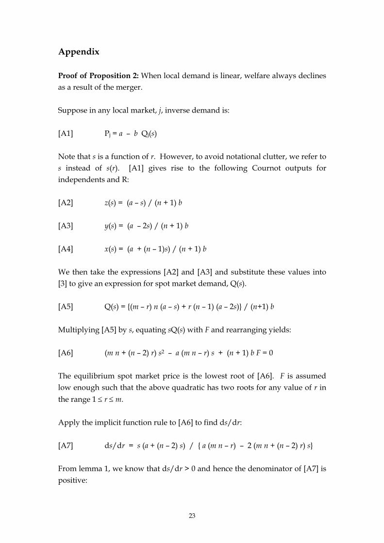
Proof of Proposition 2: When local demand is linear, welfare always declines

as a result of the merger.

Suppose in any local market, j, inverse demand is:

[A1] Pj = a – b Qj(s)

Note that s is a function of r. However, to avoid notational clutter, we refer to

s instead of s(r). [A1] gives rise to the following Cournot outputs for

independents and R:

[A2] z(s) = (a – s) / (n + 1) b

[A3] y(s) = (a – 2s) / (n + 1) b

[A4] x(s) = (a + (n – 1)s) / (n + 1) b

We then take the expressions [A2] and [A3] and substitute these values into

[3] to give an expression for spot market demand, Q(s).

[A5] Q(s) = {(m – r) n (a – s) + r (n – 1) (a – 2s)} / (n+1) b

Multiplying [A5] by s, equating sQ(s) with F and rearranging yields:

[A6] (m n + (n – 2) r) s2 – a (m n – r) s + (n + 1) b F = 0

The equilibrium spot market price is the lowest root of [A6]. F is assumed

low enough such that the above quadratic has two roots for any value of r in

the range 1 ≤ r ≤ m.

Apply the implicit function rule to [A6] to find ds/dr:

[A7] ds/dr = s (a + (n – 2) s) / { a (m n – r) – 2 (m n + (n – 2) r) s}

From lemma 1, we know that ds/dr > 0 and hence the denominator of [A7] is

positive:

24

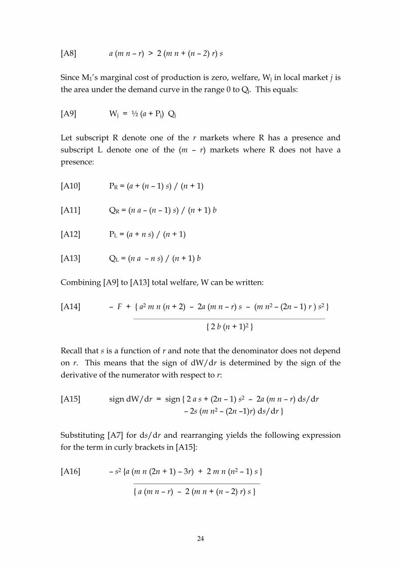
[A8] a (m n – r) > 2 (m n + (n – 2) r) s

Since M1’s marginal cost of production is zero, welfare, Wj in local market j is

the area under the demand curve in the range 0 to Qj. This equals:

[A9] Wj = ½ (a + Pj) Qj

Let subscript R denote one of the r markets where R has a presence and

subscript L denote one of the (m – r) markets where R does not have a

presence:

[A10] PR = (a + (n – 1) s) / (n + 1)

[A11] QR = (n a – (n – 1) s) / (n + 1) b

[A12] PL = (a + n s) / (n + 1)

[A13] QL = (n a – n s) / (n + 1) b

Combining [A9] to [A13] total welfare, W can be written:

[A14] – F + { a2 m n (n + 2) – 2a (m n – r) s – (m n2 – (2n – 1) r ) s2 } _______________________________________________________________________

{ 2 b (n + 1)2 }

Recall that s is a function of r and note that the denominator does not depend

on r. This means that the sign of dW/dr is determined by the sign of the

derivative of the numerator with respect to r:

[A15] sign dW/dr = sign { 2 a s + (2n – 1) s2 – 2a (m n – r) ds/dr

– 2s (m n2 – (2n –1)r) ds/dr }

Substituting [A7] for ds/dr and rearranging yields the following expression

for the term in curly brackets in [A15]:

[A16] – s2 {a (m n (2n + 1) – 3r) + 2 m n (n2 – 1) s } _______________________________________________

{ a (m n – r) – 2 (m n + (n – 2) r) s }

25

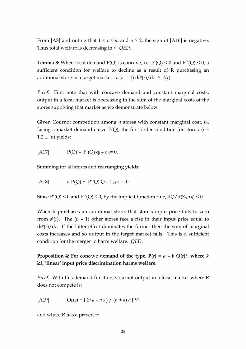
From [A8] and noting that 1 ≤ r ≤ m and n ≥ 2, the sign of [A16] is negative.

Thus total welfare is decreasing in r. QED.

Lemma 3: When local demand P(Q) is concave, i.e. P’(Q) < 0 and P’’(Q) < 0, a

sufficient condition for welfare to decline as a result of R purchasing an

additional store in a target market is: (n – 1) dsb(r)/dr > sb(r)

Proof. First note that with concave demand and constant marginal costs,

output in a local market is decreasing in the sum of the marginal costs of the

stores supplying that market as we demonstrate below.

Given Cournot competition among n stores with constant marginal cost, υi,

facing a market demand curve P(Q), the first order condition for store i (i =

1,2,..., n) yields:

[A17] P(Q) – P’(Q) qi – υi,= 0.

Summing for all stores and rearranging yields:

[A18] n P(Q) + P’(Q) Q – Σ∀i υi = 0

Since P’(Q) < 0 and P’’(Q) ≤ 0, by the implicit function rule, dQ/d(Σ∀i υi) < 0.

When R purchases an additional store, that store’s input price falls to zero

from sb(r). The (n – 1) other stores face a rise in their input price equal to

dsb(r)/dr. If the latter effect dominates the former then the sum of marginal

costs increases and so output in the target market falls. This is a sufficient

condition for the merger to harm welfare. QED.

Proposition 4: For concave demand of the type, P(r) = a – b Q(r)k, where k

≥1, ‘linear’ input price discrimination harms welfare.

Proof. With this demand function, Cournot output in a local market where R

does not compete is:

[A19] QL(s) = { (n a – n s ) / (n + k) b } 1/k

and where R has a presence:

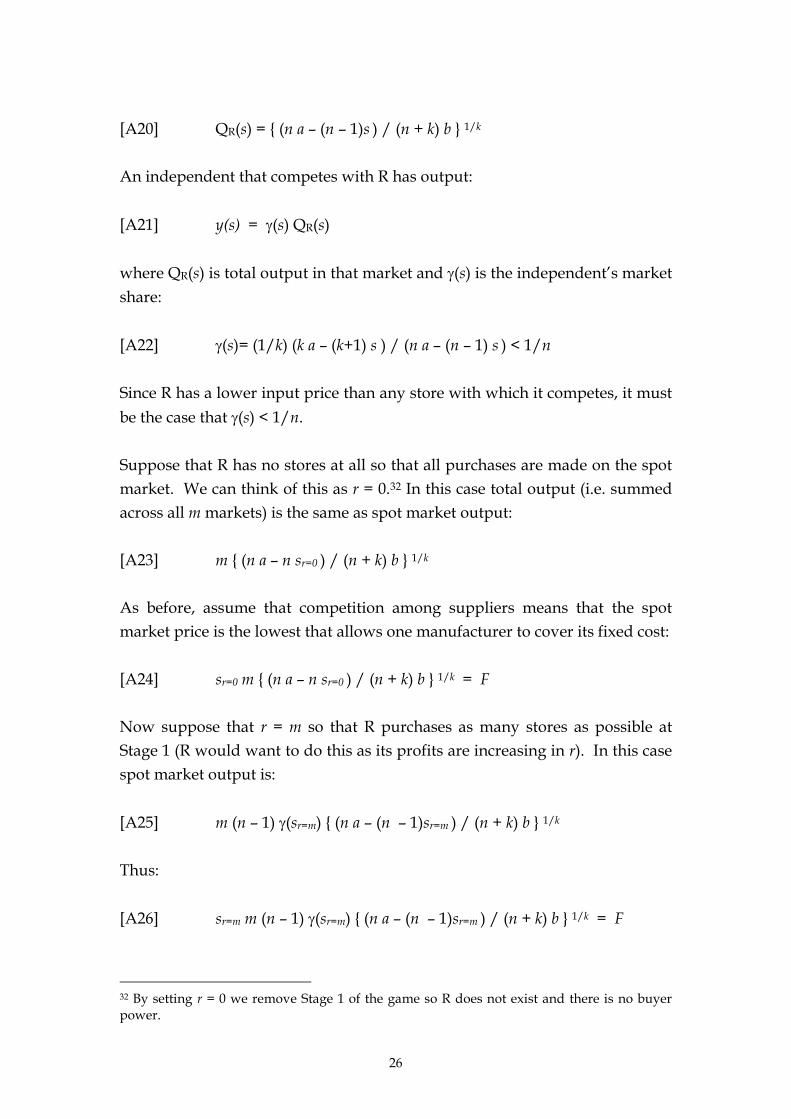
26

[A20] QR(s) = { (n a – (n – 1)s ) / (n + k) b } 1/k

An independent that competes with R has output:

[A21] y(s) = γ(s) QR(s)

where QR(s) is total output in that market and γ(s) is the independent’s market

share:

[A22] γ(s)= (1/k) (k a – (k+1) s ) / (n a – (n – 1) s ) < 1/n

Since R has a lower input price than any store with which it competes, it must

be the case that γ(s) < 1/n.

Suppose that R has no stores at all so that all purchases are made on the spot

market. We can think of this as r = 0.32 In this case total output (i.e. summed

across all m markets) is the same as spot market output:

[A23] m { (n a – n sr=0 ) / (n + k) b } 1/k

As before, assume that competition among suppliers means that the spot

market price is the lowest that allows one manufacturer to cover its fixed cost:

[A24] sr=0 m { (n a – n sr=0 ) / (n + k) b } 1/k = F

Now suppose that r = m so that R purchases as many stores as possible at

Stage 1 (R would want to do this as its profits are increasing in r). In this case

spot market output is:

[A25] m (n – 1) γ(sr=m) { (n a – (n – 1)sr=m ) / (n + k) b } 1/k

Thus:

[A26] sr=m m (n – 1) γ(sr=m) { (n a – (n – 1)sr=m ) / (n + k) b } 1/k = F

32 By setting r = 0 we remove Stage 1 of the game so R does not exist and there is no buyer power.

27

Combining [A24] and [A26] we have:

[A27] sr=0 (n a – n sr=0 )1/k = sr=m (n – 1) γ(sr=m) (n a – (n – 1)sr=m ) 1/k

Note that if welfare when r = 0 is greater than when r = m, all we need is to

show that output in a local market is higher when r = 0. If welfare is the same

when r = 0 and when r = m, it must be the case that the sum of marginal costs

in each local market is the same:

[A28] n sr=0 = (n – 1) sr=m

However, if [A28] holds, the right hand side of [A27] is smaller than the left

hand side (since, from [A22], γ(sr=m) < 1/n). To restore the balance we require

that:

[A29] n sr=0 < (n – 1) sr=m

since the left hand side of [A27] is increasing in sr=0. To see this, differentiate

the left hand side of [A27] with respect to sr=0 and note that the resulting

expression is positive if:

[A30] k a – (k + 1) sr=0 > 0

which surely holds from [A22].

From [A29] the sum of marginal costs is lower and hence output higher when

r = 0 than when r = m. Hence W(r=m) < W(r=0). QED.