waterborne erosion - an australian story - land and … erosion – an australian story nlwra atlas...
TRANSCRIPT

C S I R O L A N D a nd WAT E R
Waterborne Erosion - an Australian StoryContent for the Australian Natural Resources Atlas Storyboards
Compiled by Frances Marston
Contributors
Ian Prosser, Andrew Hughes, Hua Lu and Janelle Stevenson
CSIRO Land and Water, Canberra
Technical Report 17/01, September 2001

Waterborne erosion — an Australian story Content for the Australian Natural Resources Atlas Storyboards
Compiled by
Frances Marston
Contributers:
Ian Prosser
Andrew Hughes
Hua Lu
Janelle Stevenson
Technical Report No. 17/01
CSIRO Land and Water, July 2001.

Waterborne Erosion – An Australian Story NLWRA Atlas Storyboards Content
Compiled by Frances Marston, CSIRO Land and Water Page i
Contents
1 Introduction................................................................................... 11.1 Why bother telling a story about waterborne erosion? ...............................................................11.2 Stories .....................................................................................................................................................1
2 Waterborne erosion – some theory before practice ....................................... 22.1 Erosion processes................................................................................................................................. 2
2.1.1 Soil erosion proceses ............................................................................................................. 22.1.2 Components of the soil erosion process............................................................................. 3
2.2 Describing soil erosion processes..................................................................................................... 42.2.1 Sheetwash and rill erosion.................................................................................................... 42.2.2 Gully erosion ............................................................................................................................. 52.2.3 Streambank erosion................................................................................................................ 6
2.3 Predicting erosion................................................................................................................................. 72.3.1 Modelling sheetwash and rill erosion.................................................................................. 82.3.2 Modelling gully erosion........................................................................................................... 92.3.3 Modelling streambank erosion............................................................................................ 102.3.4 Modelling sediment transport in rivers............................................................................ 10
2.4 Terms and expressions...................................................................................................................... 12
3 The Erosion story ........................................................................... 173.1 The sheetwash and rill erosion picture ......................................................................................... 17
Continental snapshot of erosion ................................................................................................... 17Croplands ........................................................................................................................................... 19Grazing Lands....................................................................................................................................20Factors Contributing to Sheetwash and Rill Erosion............................................................... 21
Soil erodibility picture.............................................................................................................. 21Continental rainfall erosivity picture.....................................................................................22Continental perennial and woody cover and monthly ground vegetation cover.............23Length and Slope factors .........................................................................................................23
3.2 Gully erosion picture ..........................................................................................................................243.3 Streambank erosion picture.............................................................................................................26
4 The sediment delivery story ................................................................ 29Bedload accumulation ...................................................................................................................... 31Suspended sediment........................................................................................................................33Changes since European settlement ............................................................................................34Contributions to the coast.............................................................................................................35
5 Picture Thumbnails........................................................................... 37
6 References ................................................................................... 38
7 Appendix: River Basin Analysis ............................................................. 40

Waterborne Erosion – An
Australian Story Content for the Australian Natural Resources Atlas Storyboards
(A product of the National Land & Water Resources Audit)
Compiled by Frances Marston
Contributors: Ian Prosser, Andrew Hughes, Hua Lu and Janelle Stevenson
We wish to acknowledge all those who made contributions to the Project (NLWRA Theme 5.4b)
including Greg Canon, John Gallant, Alan Marks, Chris Moran, Geoff Pickup, Graeme Priestley, Paul
Rustomji, Anthony Scott, and Bill Young. Funding for the work was through a partnership between
the National Land and Water Resources Audit and CSIRO Land and Water.
Note to reader on annotations:
The main purpose of this document is to facilitate the exchange of information that may be included as content for the Australian Natural Resources Atlas Storyboards (a web-based product of the National Land & Water Resources Audit) and to fulfil some of the reporting requirements of the Sediment Project within NLWRA Theme 5.4b). However, the Atlas will probably only reproduce a subset selection of this document.
Text underlined and in green italics indicates links to glossary words in Section 2.4 (Terms and expressions).
A '☞ ' indicates a comment describing intended web functionality. Comments are not reproduced in the print version of the document.
Hypertext links are indicated with the URL or internal link underlined and in blue – if URL unknown, a descriptive title is provided
Text which is bold and navy is meant to be emphasised in some way ie it flashes, sparkles, is extra bold etc on web page.

Waterborne Erosion – An Australian Story NLWRA Atlas Storyboards Content
Compiled by Frances Marston, CSIRO Land and Water Page 2
Waterborne Erosion – An Australian Story NLWRA Atlas Storyboards Content
Compiled by Frances Marston, CSIRO Land and Water Page 1
1 INTRODUCTION
1.1 Why bother telling a story about waterborne erosion?
A major issue in Australian land management is waterborne soil erosion and the consequent
degradation of land and water resources. Because soil provides the structural support and the
source of water and nutrients for plants, soil erosion results in significant reductions in
productivity. Off-site, the effect of soil erosion is the degradation of water quality in streams,
water storages and estuaries due to increases in sediments and associated nutrients and the
consequent impacts on ecosystem health.
High concentrations of suspended sediment:
• reduce stream clarity • inhibit respiration and feeding of stream biota • diminish light needed for plant photosynthesis • require treatment of water for human use
In addition an over-supply of mud or sand can cover the stream bed and cobbles and fill deep
pools, making streams uninhabitable for many native fish and invertebrates. An increase in the
supply of silt and clay from erosion to rivers means an increase in the supply of nutrients, for in
Australian streams most nutrients are transported attached to fine mineral and organic
sediment. The storage of fine sediment in a stream increases the storage of nutrients that can
be released into the water, fuelling nuisance and toxic levels of algae and other primary
production.
Knowledge about the sources and rates of erosion under past and present conditions is
essential for understanding the consequence of changes in land use and climate on soil erosion.
This is a prerequisite for minimising the decline of soil productivity and water quality and for
optimising the use of resources for soil conservation and management and the sustainability of
land use. ☞
1.2 Stories
• How much soil is eroded from hillslopes & gullies under various land uses and
management practices? (Loss of productive capacity – ie all to do with soil loss) ☞
• How much of the soil that is eroded is transported to and reworked through rivers?
(Aquatic ecosystem impacts – ie all to do with sources and transport of sediment) ☞

Waterborne Erosion – An Australian Story NLWRA Atlas Storyboards Content
Compiled by Frances Marston, CSIRO Land and Water Page 2
2 WATERBORNE EROSION – SOME THEORY BEFORE
PRACTICE
Sediment and attached nutrient that are transported in streams can be derived from two types
of processes: sheetwash and rill erosion processes on hillslopes and erosion of the streams
themselves, including recently formed stream channels such as gullies. Distinction between
hillslope and gully erosion is important for three reasons outlined below. [SoilPic 1 & 2]. ☞
1. Sediment eroded from stream banks is delivered immediately to the stream and
consequently impacts on instream ecosystems. In contrast, much sediment
generated from sheetwash and rill erosion is deposited on footslopes, alluvial fans
and terraces before reaching the stream. [SoilPic 3, 4, 5 & 6]. ☞
2. Sheetwash, rill and gully erosion entail quite different management approaches.
Streambank and gully erosion is best targeted by managing stock access to streams,
protecting vegetation cover in areas prone to future gully erosion, revegetating bare
banks and reducing sub-surface seepage in areas with erodible sub-soils. Sheetwash
and rill erosion is best targeted by promoting consistent groundcover, maintaining
soil structure, promoting nutrient uptake and using riparian buffer strips. [SoilPic 7].☞
3. Sheetwash and rill erosion can respond to short-term changes in land management,
and trends are often reversible, whereas gully erosion reacts over longer time scales,
and is mostly in response to the major clearing of vegetation upon introduction of
modern land use. Gully erosion tends to go through a trend of rapid initial change and
then gradual adjustment to a new equilibrium condition.
It is important to keep in mind that erosion does occur as a natural process – but accelerated
rates of erosion occur as a consequence of human intervention.
2.1 Erosion processes
Erosion is the process by which the earth's surface is worn away by the action of water, wind,
glaciers, waves etc. It can be natural (ie due only to the forces of nature) or accelerated (as a
result of human activities) but in each case the same processes operate and the distinction is
often only a matter or degree and rate.
2.1.1 Soil erosion proceses
Soil erosion processes (sheetwash and rill, gully, streambank, and wind erosion; mass movement;
and solution) operate in conjunction to denude the earth's surface of weathered material. The
first three processes (sheetwash and rill, gully, and streambank erosion) are considered in detail
in this project. Wind erosion is also a significant process in dry areas but was beyond the scope

Waterborne Erosion – An Australian Story NLWRA Atlas Storyboards Content
Compiled by Frances Marston, CSIRO Land and Water Page 3
of the NLWRA, and mass movement (landsliding and soil creep) and solution are minor processes
in terms of accelerated erosion.
2.1.2 Components of the soil erosion process
There are three main components of the erosion process:
! Detachment ! Transport ! Deposition
Detachment of soil particles is a function of the erosive forces of raindrop impact and flowing
water, the susceptibility of the soil to detach, the presence of plant cover or other roughness
which reduces the magnitude of the eroding forces and management of the soil that makes it
less susceptible to erosion. It occurs when the erosive forces of raindrop impact or of flowing
water exceed the soil's resistance to erosion. Other detachment processes by soil organisms
such as ants or burrowing animals can be significant in places.
Transport is the entrainment and movement of sediment from its original location once it has
been detached from the soil. It is a function of the energy of the transporting agent, in this
case flowing water. Deep and fast flows have a greater capacity to transport sediment, and fine
particles are moved more easily than larger and heavier particles. Deposition occurs when the
sediment load of a given particle type exceeds the energy available for transport or re-
entrainment. This often results from a reduction in gradient, flow velocity or discharge or an
increase in the hydraulic resistance of the flow induced by vegetation. Deposition results in
sedimentation.
Sediment yield is the amount of material transported past a given point of interest (usually a
measuring device in a stream or a point on a hillslope). It is the net result of erosion, transport
and deposition upstream or upslope.
Sediment delivery ratio is usually described as the ratio at a particular point of gross erosion
upstream or upslope to the sediment yield at that point. It is a measure of the efficiency of
transport and conversely of the intensity of deposition upstream or upslope. The above
definition is not strictly correct because gross erosion is rarely measured. Typically sediment
yield of hillslope plots is the measure of erosion. Then, sediment delivery ratio is the reduction
in sediment yield per unit area with an increase in scale from plot to hillslope, stream or river.
Soil eroded by water is transported downslope by surface runoff, which is the portion of rainfall
that flows over the ground or in streams as opposed to infiltrating the soil or being lost to
evaporation.
(Much of the above is based on Sharman & Murphy, 1991)

Waterborne Erosion – An Australian Story NLWRA Atlas Storyboards Content
Compiled by Frances Marston, CSIRO Land and Water Page 4
Figure 1: Sediment yields from rill and
sheetwash erosion under various landuses.
2.2 Describing soil erosion processes
To measure erosion and sediment transport processes for every catchment where sediment
supply is of concern is an enormous and unnecessary task. Fortunately, with knowledge of the
processes, surrogate factors can be measured to estimate soil erosion, sediment yields, and
deposition across a diverse range of environments.
2.2.1 Sheetwash and rill erosion
The factors controling sheetwash and rill erosion are well understood from decades of soil
erosion research. The most significant factors are surface cover and land use practise.
Significant sheetwash erosion occurs when contact cover with the ground falls below 70%, and is
particularly pronounced when cover falls below 30%. Consequently any land use that includes
annual tillage and seasonal bare ground is prone to surface wash erosion. The strong effects of
land use intensity on hillslope erosion are illustrated by the data in Figure 1. The graph shows a
review of plot and mini catchment scale measurements of sheetwash and rill erosion in Australia.
Sheetwash and rill erosion is accentuated
by high rainfall intensity, particularly if it
occurs when the soil is bare. A large
depth of rainfall over a short period of
time as occurs in summer storms, is much
more erosive than gentle continuous
drizzle. Thus there is a tendency in
Australia for sheetwash and rill erosion to
increase as one moves north, where
rainfall intensities are higher. The
difference between sediment yields for
wheat on the Darling Downs compared to
SE Australia illustrates this. Steep
gradients and erodible soils further
accentuate erosion. Soil properties are
particularly important for nutrient loss as
much of the nutrient is attached to silt and clay. On poorly structured soils, silt and clay tend to
be transported as individual particles rather than in larger aggregates. This increases the travel
distance and the difficulty of trapping eroded sediment. ☞
A feature of sheetwash and rill erosion is the huge variability of sediment yields. Within a
single landuse sediment yields vary by 100 fold depending upon rainfall, topography and
management practice. Between landuses, the data suggest 10,000 fold differences between
locations. Strong patterns emerge within this variation when controlling factors are considered.

Waterborne Erosion – An Australian Story NLWRA Atlas Storyboards Content
Compiled by Frances Marston, CSIRO Land and Water Page 5
In terms of sediment delivery potential to streams, the potential for the eroded sediment to
actually reach the stream must be considered. Consequently, areas where hillslopes fall straight
into the stream have the highest sediment delivery potential. This usually results in higher
sediment delivery potential to small source streams rather than directly over the banks of major
rivers and creeks.
There is sufficient understanding of the sheetwash and rill erosion processes that a technique
known as the Revised Universal Soil Loss Equation (RUSLE) has been developed to predict this
kind of erosion at regional scales, on the basis of the primary driving factors. ☞
2.2.2 Gully erosion
Quite different considerations need to be made for gully and streambank erosion because of the
tendency for erosion to heal over time. Gullies and incised streams increase the extent and size
of the stream network creating large areas of bare eroding banks.
The factors which dictate sediment yield from gullies are not as well understood as for
sheetwash and rill erosion. There is no equivalent of the RUSLE for gully erosion, however there
is enough understanding of the processes to make regional assessments using some strategic
measurements. ☞
Gullies have formed in valleys which contained no channels, or only small channels, prior to
European settlement. Thus the total volume of gully represents the total amount of sediment
delivered from gully erosion in historical times. There are vast differences in gully density from
one area to another and this is the primary factor dictating the total amount of sediment
yielded from gully erosion since European settlement, and is the basis of our assessment of
sediment yield. Gully density can be converted to mean annual sediment load using average
width, depth and age of gullies.
Gullies erode deep soils that
accumulate in valleys and hollows from
thousands of years of upslope
sheetwash erosion and soil creep.
Once the protective vegetation cover
or resistant topsoil layers are
removed, gullies spread rapidly up
through the valleys towards the
surrounding ridges and spurs where
they stop due to insufficient runoff
to continue erosion. Thus gullies
spread quickly once initiated but
stabilise relatively quickly despite the continuing dramatic appearance of a deep bare scar on the
landscape. In areas cleared long ago, such as in the late 19th century for the uplands of the
Figure 2 (based on Wasson et al. 1998)

Waterborne Erosion – An Australian Story NLWRA Atlas Storyboards Content
Compiled by Frances Marston, CSIRO Land and Water Page 6
MDB, the bulk of the eroded soil was delivered to streams in the first few decades and
sediment yield has since declined (Figure 2). Measurements of gully density in those areas show
little net growth of the network since the 1940s. In other areas of currently intensifying land
use, such as the tropical semi-arid grazing lands many gullies are still forming and continuing to
expand.
Many old gullies still generate turbid water and this is most accentuated where there are highly
erodible sodic sub-soils that are quite inhospitable for regeneration of vegetation.
2.2.3 Streambank erosion
There are many similarities between gully and streambank erosion but our understanding of the
primary factors which control the rate of streambank erosion are even more limited and are the
subject of current research. It is known that there has been massive widening of many of our
coastal streams in historical times as a results of clearing of riparian vegetation, increased flood
magnitudes and increase of flow velocities through activities such as the removal of large woody
debris. This has been shown most dramatically by contrasting the Thurra and Cann rivers in East
Gippsland. These are rivers draining similar catchments. The main difference is that much of
the lower Cann River floodplain has been cleared while the Thurra River remains relatively
pristine. Meander cutoffs on the Cann River confirm that it was similar to the Thurra River
prior to European settlement. Table 1 shows a four times increase in the width of the Cann
River, about a two and a half time increase in depth and a 63 times increase in bankfull discharge
in historical times. These changes have supplied a vast amount of sediment downstream and have
impacted the bed habitat of the lower Cann River.
Table 1: Contrasts in channel form and sediment transport between Thurra River (unaltered in historical times) and the
adjacent Cann River (eroded in historical times). After Prosser et al. (2001); data from Brooks (1999).
Parameter Thurra R. Cann R.
Channel width (m) 13 66
Channel depth (m) 1.4 4
Bank height as a proportion of critical height for failure 0.29 0.9
Bankfull discharge (m3s-1) 10 630
Unit stream power (W m-2) 10 153
Bedload transport potential (kg s-1) 0.6 325
Lateral migration rate (m year-1) 0.07 4.5
Measurements of streambank erosion from around the world show a relationship between
bankfull discharge and streambank erosion rate (Rutherfurd, 2000) indicating that large rivers
erode at a faster rate than smaller streams. It is understood that most current problems of
bank erosion are in reaches where the native riparian vegetation has been removed. Reaches

Waterborne Erosion – An Australian Story NLWRA Atlas Storyboards Content
Compiled by Frances Marston, CSIRO Land and Water Page 7
with natural riparian vegetation are more stable. It has been shown that riparian tree roots
provide sufficient strength to stabilise the majority of river banks (Abernethy and Rutherfurd,
2000). These principles were used to predict bank erosion rate under current conditions.
2.3 Predicting erosion
Measurement of soil erosion is time consuming and constrained by severe data limitations. There
are large gaps in erosion mesurement in terms of regions and particular environmental conditions
assessed. The only way to cover these gaps and provide a regionally comprehensive assessment
is to use the data and that gathered elsewhere to predict erosion based upon more widely
measured surrogate factors such as climate, land use, soil properties and topography. The
stories and predictions presented in these pages about soil loss and sediment movement are the
outputs of sophisticated modelling routines based upon intensive assessment of available data.
They describe findings generated within a spatial modelling framework on a continental scale
for an area defined as Australian river basins containing intensive agriculture (ARBIA).
This area encompasses locations of intensive land use in Australia and their surrounding
catchments to make a largely contiguous area. Geographically, it is the catchments of the
Australian east coast (extending from Cape York to the Eyre Peninsula), Tasmania, the south
west of Western Australia, and the Ord Basin. For this project the Ord Basin and Western
Plateau drainage divisions were excluded due to lack of information. Complete catchments are
used to put intensive land use in the context of the catchments in which it is located. The
assessment area consequently includes much non-intensive land use such as forestry and
rangelands. Much of the sheetwash and rill erosion work was undertaken across the whole
continent as data covered that whole area.
The assessment area has been divided into regions to assist the storytelling process. ☞
Maps have been prepared for: ☞
• Current levels of continental soil loss from sheetwash and rill erosion ☞ • Natural levels of continental soil loss from sheetwash and rill erosion ☞ • Difference between current and natural levels of continental soil erosion ☞
Map 1: For the modelling
exercise the assessment area
was divided into regions
(based on river basins) for
which much of the data is
presented. This provided a
useful reporting mechanism.

Waterborne Erosion – An Australian Story NLWRA Atlas Storyboards Content
Compiled by Frances Marston, CSIRO Land and Water Page 8
• Continental soil erodibility ☞ • Continental rainfall erosivity ☞ • Continental ground cover ☞ • Continental soil erosion from gully erosion ☞
2.3.1 Modelling sheetwash and rill erosion
The controls on hillslope erosion by sheetwash and rill erosion are well understood and there are
several models which incorporate these factors. Our modelling is based on the Revised Universal
Soil Loss Equation (RUSLE) using time series of remote sensing imagery and daily rainfall
combined with updated spatial data for soil, land use and topography.
The RUSLE calculates mean annual soil loss (tonnes/ha/yr) as a product of six factors: rainfall
erosivity, soil erodibility, hillslope length, hillslope gradient, ground cover and land use practice.
The factors included in the RUSLE vary strongly across the Australian continent, providing a
method for estimating the spatial patterns of erosion using consistent information for each
factor. Due to the lack of spatial data for contour cultivation and bank systems, an assessment
of the land use practice factor is excluded. This has the effect of not predicting reductions in
soil loss due to use of minimum tillage and other conservation practises in intensive land use
areas. This limitation is taken into account when discussing then results.
Mean annual values for rainfall erosivity and ground cover are often used to calculate mean
annual hillslope erosion. This neglects important seasonal patterns of rainfall erosivity and
cover. Problematic to the standard annual application of the RUSLE is the pronounced wet-dry
precipitation regime in Australia's tropics and Mediterranean climate areas. To adequately
represent the erosive potential of rainfall for each temporally distinct period, the study applied
the RUSLE model on a monthly averaged basis, calculating appropriate erosivity and cover
factors for each month. Twenty years (1980-1999) of daily rainfall data mapped across
Australia and 13 years (1981-1994) of satellite vegetation data were used for this purpose.
Incorporation of seasonal effects reduces predicted mean annual soil loss in Australia's tropics
by a factor of 1.5.
The predictions of sheetwash erosion under present land use need to be put in context of
erosion under natural vegetation cover. We predicted natural erosion using the same procedure,
with a cover factor for native vegetation and keeping the other factors of soil erodibility,
rainfall erosivity and topography as for the present day.
The cover factor for native vegetation was obtained assessing areas of reserve where native
vegetation cover is retained in each of Australia’s native vegetation zones. In the reserves, the
RUSLE C factor was determined from remote sensing data as part of the assessment of current
soil loss. The native vegetation cover of these reserve areas was extrapolated across the river
basins containing intensive agriculture using an empirical decision tree model based on climatic

Waterborne Erosion – An Australian Story NLWRA Atlas Storyboards Content
Compiled by Frances Marston, CSIRO Land and Water Page 9
topographic, and geological factors. The cover management factor for areas not contained
within the assessment area remained unchanged.
The acceleration of current mean annual soil loss above natural rates was predicted as the ratio
of the current to pre-European mean annual soil loss predictions.
For a full technical description of the modelling procedure see Technical Document PDF. ☞
2.3.2 Modelling gully erosion
Three separate data sources were used to map the density of gullies throughout the river basins
containing intensive agriculture. For NSW, the data from the NSW 1988 land degradation
survey were used (Graham, 1989). These are measurements of gully density (kilometre of gully
length per km2 of land) from aerial photographs across NSW. The measurements were taken on
a regular grid of 5 to 10 km spacing across NSW. At each point an erea of 1 km2 was measured.
We found that this area was small compared to the spacing of gullies. There was thus much
variation in the data even within a small region as some sample points were on top of hills, where
gullies do not form and at the other extreme were sample points at valley junctions which
contained small networks of gully. Consequently the data only represented coherent and
predictable patterns of erosion if averaged over a large area. We found that the best results
were achieved by averaging the data across 40 x 40 km cells.
For Victoria, an existing polygon map of gully density was provided by DNRE based upon mapping
by Lindsay Milton and others (Ford et al., 1993). This is also at fairly coarse scale consisting of
33 polygons across the state.
No existing data were available for the rest of the assessment area so gullies were traced on
more than 428 stereo pairs of aerial photographs sampled from the other States. These data
were digitised and used to build a decision tree model of gully density. The decision tree model
estimated gully density for the entire assessment area in terms of the known gully densities
(measured from the aerial photographs) and environmental attributes available at the
continental scale. For example, the model was able to determine that areas with granitic
lithology, moderate hillslope gradient and moderate to high rainfall are likely to have higher gully
densities than an area of similar geology and rainfall but lower hillslope gradients. Numerous
environmental attributes were used to determine which environmental attributes had the
greatest predictive ability in terms of gully density. Attributes used included land use, geology,
soil texture, rainfall and indices of seasonal climate extremes. Because of the inability to
detect gullies in forested areas from aerial photographs and the fact that gullies are less likely

Waterborne Erosion – An Australian Story NLWRA Atlas Storyboards Content
Compiled by Frances Marston, CSIRO Land and Water Page 10
to occur in forested areas, a gully density value of zero was applied to all areas with forest
cover.
Three separate models were generated from the data, based upon geographic areas: West
Australia; South Australia and Tasmania; and coastal Queensland. A model for the northern part
of Australia (including parts of the Northern Territory and north Western Australia) was
attempted, however, an inadequate number of high quality aerial photographs prohibited the
generation of accurate results.
For a full technical description of the modelling procedure see Technical Document PDF. ☞
2.3.3 Modelling streambank erosion
All streams with a catchment area greater than 50 km2 and a length greater than 5 km were
mapped over the assessment area using the national 9" digital elevation model. The proportion
of each stream that has cleared native riparian vegetation was determined by intersection of
the streams with a coverage of native vegetation in 1995 obtained from the Australian Land
Cover Change project at a resolution of 100 m (http://www.brs.gov.au:80/land&water/landcov/alcc_results.html).
This is the best available data but it is only a crude measure of riparian condition as the 100 m
resolution fails to identify narrow bands of remnant riparian vegetation in cleared areas but it
also fails to identify narrow valleys of cleared land penetrating otherwise uncleared hills.
Erosion was assumed to only occur on sections of river with cleared riparian vegetation. The
mean annual rate of bank erosion was calculated by:
400080 .. bQBE =
(modified from Rutherfurd, 2000) where BE is bank erosion rate in m/y; and Qb is bankfull
discharge, estimated from gauging records across the assessment area. Bankfull discharge was
assumed to be equal to a flow of recurrence interval of 1.6 y. Multiplying the bank erosion rate
by the length of cleared bank and an assumed average bank height of 3 m and bulk density of 1.5
t/m3 gives the mean annual supply of sediment from bank erosion to each stream link in t/y.
For a full technical description of the modelling procedure see Technical Document PDF. ☞
2.3.4 Modelling sediment transport in rivers
Much of the sediment moving on hillslopes is deposited before reaching the stream, often on
footslopes or in riparian lands. We obtained the most satisfactory results of river sediment
transport by assuming that only 5-10% of sheetwash and rill erosion was delivered to streams;
that is a hillslope sediment delivery ratio of 5-10%. This accords broadly with observations of
hillslope and small catchment sediment yields. Sediment from gully and streambank erosion is
delivered more efficiently, but little of the sediment that has reached streams over historical

Waterborne Erosion – An Australian Story NLWRA Atlas Storyboards Content
Compiled by Frances Marston, CSIRO Land and Water Page 11
times has been yielded to the coast. It is a widely held observation that much of the sediment
is stored along the way on floodplains or on the stream bed. When substantial sediment is
deposited on the stream bed it can have an impact on aquatic ecosystems. Floodplain deposition
in billabongs and other features may also be detrimental, however, it has the benefits of
protecting downstream reaches and the coast from receiving that sediment. This is a benefit
when current rates of sediment supply are accelerated above natural rates.
Individual stream links have widely varying potential for deposition because of strong
differences in the energy of flow and the extent of floodplains. The crucial aspect of modelling
sediment transport through rivers is to predict the patterns of deposition through the river
network in addition to the supply of sediment to the rivers.
The sediment sources described in Section 2.2 deliver both coarse and fine grained sediment to
streams. These are treated separately within the river network because of their different
transport processes and different impacts on rivers. Fine sediment is transported in suspension
in the river flow. When flood flows overtop the banks they spread onto the floodplain and a
proportion of suspended sediment goes with that overbank flow. Floodplain flows are relatively
shallow and slow flowing. In many cases the flow is retained on the floodplain for several days.
Under these conditions much of the suspended sediment has time to settle out of the flow and
be deposited on the floodplain. The amount of sediment that settles on the floodplain was
predicted as a function of the mean sediment concentration and the ratio of floodplain area to
overbank discharge.
Flows within the stream are generally too fast for there to be any net accumulation of
suspended sediment from year to year and the within channel sediment is delivered quickly
downstream. Rivers have a capacity to transport vast quantities of suspended sediment
particularly during floods and the concentration of sediment in Australian rivers, and rivers in
general, is limited by the supply of the sediment to the river; that is, if the amount of sediment
supplied is doubled then the river will be able to carry the extra load and the sediment
concentration will be doubled.
Coarse sediment is transported along the bed of the stream by rolling and relatively short hops
into the flow. Under very fast, deep flow their may be brief periods of suspension. The
sediment moves much slower than the flow and generally moves 10s to 100s of metres during an
individual flood, accumulating on the bed of the stream between floods. The capacity of streams
to transport coarse sediment is quite limited and accelerated sediment supply can exceed the
capacity of the stream to convey sediment downstream. Under such conditions there is net
accumulation of excess sediment on the bed of the stream, covering the natural substrate. The
total amount accumulated over historical times is the amount of coarse sediment supplied less
the total capacity to transport coarse sediment downstream. The capacity to transport coarse
sediment is a function of the river slope and its discharge regime. Accumulation of coarse sand
and fine gravel has been extensive in historical times.

Waterborne Erosion – An Australian Story NLWRA Atlas Storyboards Content
Compiled by Frances Marston, CSIRO Land and Water Page 12
A mean annual sediment budget was constructed through each river network for the river basins
containing intensive agriculture. Separate budgets were constructed for coarse and fine
sediment. The sediment budget accounts for the supply of sediment to each stream link and
deposition within the link. The remaining sediment is yielded to the next link downstream. The
sediment budget was conducted sequentially from the top of each catchment to the mouth.
Coarse sediment is derived from gully erosion, streambank erosion and sediment yield from
tributaries. Supply of coarse sediment directly from hillslopes to rivers was assumed to be
negligible. Fine sediment is derived from sheetwash and rill erosion, gully erosion, streambank
erosion and tributary sediment supply. Streambank and gully erosion were predicted to yield an
equal proportion of fine and coarse sediment. This conforms with observations and produced
realistic sediment budgets for each component. Fine sediment dominates the sediment yield as
one moves through the river network because of its faster transport, and lower residence time
in the river network.
Deposition within reservoirs was considered in addition to floodplain deposition of suspended
sediment and instream deposition of coarse sediment. The trap efficiency of reservoirs was
calculated from the widely used Brune rule (Brune, 1953) based upon the ratio of mean annual
flow to reservoir storage capacity. Most of the larger reservoirs in Australia trap 90% or more
of incoming sediment, and thus strongly modify sediment delivery downstream.
For a full technical description of the modelling procedure see Technical Document PDF. ☞
2.4 Terms and expressions
Alluvial Fan
Material deposited by a stream where it emerges from the constriction of a valley to a plain.
(From Whittow, 1986)
Assessment Area
The river basins containing intensive agriculture form the basis of the assessment area for this
and several other NLWRA projects dealing with agriculture and catchment processes. It
encompasses locations of intensive land use in Australia and their surrounding catchments to
make a largely contiguous area. Geographically, it is the catchments of the Australian east coast
(extending from Cape York to the Eyre Peninsula), Tasmania, the south west of Western
Australia, and the Ord Basin. For this project the Ord Basin and Western Plateau drainage
division were excluded due to lack of information. Complete catchments are used to put
intensive land use in the context of the catchments in which it is located. The assessment area
consequently includes much non-intensive land use such as forestry and rangelands.
Waterborne Erosion – An Australian Story NLWRA Atlas Storyboards Content
Compiled by Frances Marston, CSIRO Land and Water Page 13
Detachment
Detachment of soil particles is a function of the erosive forces of raindrop impact and flowing
water, the susceptibility of the soil to detach, the presence of plant cover or other roughness
which reduces the magnitude of the eroding forces and management of the soil that makes it
less susceptible to erosion. It occurs when the erosive forces of raindrop impact or of flowing
water exceed the soil's resistance to erosion. Other detachment processes by soil organisms
such as ants or burrowing animals can be significant in places.
Digital Elevation Model (DEM)
A geographic grid of an area where the contents of each grid cell represents the height of the
terrain in that cell. Consists of X, Y and Z coordinates.
Erosion
Erosion is the continuing geomorphological process involved in landscape development as a
smoothing or levelling of the earth's surface by removal of weathered material.
It can be natural (ie due only to the forces of nature) or accelerated (as a result of human
activities) but in each case the same processes operate and the distinction is often only a matter
or degree and rate.
(Based on Sharman & Murphy, 1991)
Footslope
The lower part of a slope above the gentler gradient of a valley floor or plain.
(From Whittow, 1986)
Geomorphological Processes
Processes which comprise the physical and chemical interactions between the Earth's surface
and the natural forces (gravity, ice, water, wind, waves, etc) acting upon it to produce landforms.
Gully Density
The linear extent of gully, measured as kilometres of gully per km2 of land.
Gully Erosion
The removal of soil by running water which results in the formation of deep channels – gullies –
which tend to form in upland areas, have steep sides which often have headward eroding scarps,
and usually convey ephemeral runoff to relatively small drainage areas. Gullies are at least 50 cm
deep. Gullies erode unchanneled valleys and dips and eventually become vegetated and infill,
distinguishing them from permanent streams.
(Sharman & Murphy, 1991)

Waterborne Erosion – An Australian Story NLWRA Atlas Storyboards Content
Compiled by Frances Marston, CSIRO Land and Water Page 14
Headcuts
A sharp ephemeral waterfall cut into soil at the head of a gully or incised stream. Over time the
headcut migrates headward by scour and toppling of the soil.
Hillslope
All the land surface above a stream or channel edge.
Incised Streams
Permanent streams which have deepened and widened by several metres as a result of
vegetation removal or increased forces of flow to produce streams with high, bare vertical banks
with headcuts incised into floodplains. They resemble large gullies.
Recurrence Interval
The flow expected to occur on average every 1.6 y based upon analysis of peak flows in each year
of gauging record.
Revised Universal Soil Loss Equation (RUSLE)
Like the USLE, the RUSLE calculates mean annual erosion (tonnes/ha/yr) as a product of the six
factors: rainfall erosivity, soil erodibility, hillslope length, hillslope gradient, ground cover and
land use practice. However because the original slope steepness factor of the USLE
overestimates erosion from slopes steeper than 9%, the RUSLE applies a different slope
steepness equation in determining the hillslope gradient factor.
Related term: Universal soil loss equation (USLE).
Rill Erosion
Similar to sheetwash erosion except that the concentrated wash process causes the formation
of tiny channels or rills, a few centimetres to 50 cm deep, which usually only carry water during
storms and are removed by tillage.
Sediment
Solid material (predominantly particles and grains of rock) that have been transported by water
and deposited or settled out of suspension.
Sediment Delivery Ratio (SDR)
Sediment delivery ratio is usually described as the ratio at a particular point of gross erosion
upstream or upslope to the sediment yield at that point. It is a measure of the efficiency of
transport and conversely of the intensity of deposition upstream or upslope. The above
definition is not strictly correct because gross erosion is rarely measured. Typically sediment
yield of hillslope plots is the measure of erosion. Then, sediment delivery ratio is the reduction
in sediment yield per unit area with an increase in scale from plot to hillslope, stream or river

Waterborne Erosion – An Australian Story NLWRA Atlas Storyboards Content
Compiled by Frances Marston, CSIRO Land and Water Page 15
Sediment Transport
Transport is the entrainment and movement of sediment from its original location once it has
been detached from the soil. It is a function of the energy of the transporting agent, in this
case flowing water. Deep and fast flows have a greater capacity to transport sediment, and fine
particles are moved more easily than larger and heavier particles. Deposition occurs when the
sediment load of a given particle type exceeds the energy available for transport or re-
entrainment. This often results from a reduction in gradient, flow velocity or discharge or an
increase in the hydraulic resistance the flow induced by vegetation. Deposition results in
sedimentation.
Sediment Yield
The amount of material transported past a given point of interest (usually a measuring device in
a stream or a point on a hillslope). It is the net result of erosion, transport and deposition
upstream or upslope.
Sheetwash or Surface Wash Erosion
The removal of a relatively uniform layer of soil by raindrop splash and/or by diffuse surface
runoff during intense storms. On land where soil is not protected by a surface cover, soil is lost
from most of the land surface by sheetwash erosion.
(Based on Sharman & Murphy, 1991)
Soil Creep
(Sometimes) imperceptible slow but continuous movement or displacement of soil or subsoil,
evidenced by leaning trees and fences and bowed walls.
Streambank Erosion
The removal of soil from streambanks by the direct action of water in the channel. Typically it
occurs under high flow conditions by scour and mass failure processes, and particularly by
undercutting of the toe of the bank.
Sodic Soil
Typically sodic soils are considered unstable and, as a consequence, have high erodibility and
often present problems for soil conservation strategies. This is because the exchangeable
sodium percentage (ESP), which is a measure of the cation exchange capacity occupied by sodium
ions, of the fine earth soil material is 6 or greater.
Stream Link
The division of a river into lengths of stream between tributary junctions.

Waterborne Erosion – An Australian Story NLWRA Atlas Storyboards Content
Compiled by Frances Marston, CSIRO Land and Water Page 16
Surface Runoff
Most soil eroded by water is transported downslope by surface runoff, which is the portion of
rainfall that becomes surface flow.
Terrace
A flat or gently inclined land surface bounded by a steeper ascending slope on its inner margin
and a steeper descending slope on its outer margin.
(From Whittow, 1986)
Universal Soil Loss Equation (USLE)
The USLE calculates mean annual erosion (Y, tonnes/ha/y) as a product of six factors: rainfall
erosivity factor (R), soil erodibility factor (K), hillslope length factor (L), hillslope gradient
factor (S), ground cover factor (C) and land use practice factor (P):
Y = RKLSCP
The precise form of each factor is based on soil loss measurements on hillslope plots, mainly in
the USA.
Related term: Revised universal soil loss equation (RUSLE).

Waterborne Erosion – An Australian Story NLWRA Atlas Storyboards Content
Compiled by Frances Marston, CSIRO Land and Water Page 17
3 THE EROSION STORY
Managing the on-site impacts of soil erosion requires a comprehensive understanding of the
major erosion processes of sheetwash and rill erosion, gully erosion and streambank erosion.
Modelling these provides predictions about overall patterns of soil erosion and associated
conditions.
3.1 The sheetwash and rill erosion picture
The assessment of erosion from sheetwash and rills is based upon combining the influence of
several environmental and land use factors which determine the broad regional patterns of
erosion. The most significant of these, as required for the RUSLE model, are:
• soil erodibility • rainfall erosivity • land cover • slope gradient • slope length
These factors are used to determine regional patterns of erosion, based upon an extensive
database of erosion plot studies and national geographical information on soils, topography, and
remote sensing. Each of the geographical layers has a degree of uncertainty at any particular
place as a result of resolution and measurement limitations but they produce coherent large
scale patterns because of the huge variation in factors across large areas. Because of the
limitations of accuracy and resolution, the results should not be used at any finer scale than sub-
catchments of 25 km2 or so. To accurately assess soil erosion from any individual paddock or
farm, measurements need to be made on the farm of the local soil properties, land use and
topography.
Continental snapshot of erosion
Modelling produced a geo-referenced annual averaged soil erosion map and its monthly
distributions.
Map 2
The predictions show broadscale patterns of
annual soil erosion under contemporary landuse
(potential hillslope erosion) with the northern
part of the continent having higher erosion
potential than the south. There is also a zone
of high potential soil erosion on the western
slopes of NSW. These patterns reflect
seasonal effects. In the north, summer has

Waterborne Erosion – An Australian Story NLWRA Atlas Storyboards Content
Compiled by Frances Marston, CSIRO Land and Water Page 18
the most erosive rain, when it can coincide with relatively little ground cover and produce high
erosion potential. In southern Australia the opposite occurs, with winter being the most erosive
season but where rains falls on well vegetated land. This produces the quite strong north-south
gradient shown in the map and the tendency for summer soil erosion shown in Figure 3 below.
The results are described as representing soil erosion potential for two reasons. First, no
assessment could be made of the reduction in soil erosion under some cropping land uses as a
result of conservation practices such as minimum tillage and stubble retention. Second, in parts
of southern Australia, the naturally high soil erosion potential on steeper slopes has resulted in
soils with significant stone and rock cover, which reduces the actual rate of erosion. Again there
was no data available to model this phenomenon.
Monthly Total Erosion (millions tonnes/year)
0
200
400
600
800
1,000
1,200
1,400
Jan Feb Mar Apr May Jun Jul Aug Sep Oct Nov Dec
Month
mill
ions
t/y
Figure 3: Continental Erosion
The following observations can be made by examining the modelled predictions:
• Potentially 1.5 billion tonnes of soil is moved annually on hillslopes. • The average soil erosion rate is 2.2 tonnes/ha/year. • 62% of the continent experiences low erosion, only 1% faces high erosion and 37% of the
continent experiences medium hillslope erosion potential using the boundaries defined in Table 2. ☞
• Overall, 10% of the area is eroded at a rate greater than the continent average rate. This shows the value in targeting erosion control to particular problem areas.
• Under any given rainfall regime, the map shows that the reduction of protective ground cover increases the risk of high rates of erosion.
Table 2: Erosion Rates
Erosion Rate Tonnes/ha/year
Low < 0.5
Medium 0.51 – 9.9
High > 10

Waterborne Erosion – An Australian Story NLWRA Atlas Storyboards Content
Compiled by Frances Marston, CSIRO Land and Water Page 19
Having trouble visualising the quantities of soil under consideration?
The average 6-wheel tip truck carries about 12 tonnes. Each truck load would remove a bit less than one
millimetre of soil from the MCG (which is 20,000m2 or 2 ha) at a rate of 6 t/ha/y. Less than a millimetre
would be hard to detect each year but maintained over 30 y of continuing soil erosion makes 27 mm of soil.
Remembering that this is the most fertile part of the soil in which most of the roots live, the impact on
management would be significant.
To understand current issues of land degradation it is necessary to compare the predictions of
current soil erosion potential to that of pre-European settlement conditions under native
vegetation cover, for some areas may have naturally high erosion rates.
The map of pre-European soil erosion produces the same broad pattern of relatively high soil
erosion potential in northern Australia and much lower rates in southern Australia (Map 3). The
gross pattern of contemporary soil erosion potential reflects the natural distribution of soil
erosion across the continent. Within each climatic zone there are areas of significantly
accelerated contemporary erosion potential shown by the ratio of contemporary to natural
erosion potential (Map 4). These are areas where cover has been reduced at least seasonally. For
example, although the overall erosion rate is low in the wheat belt of WA it is still many times
higher than the naturally very low rate. Similar results are found for the cereal crop belt from
Victoria through to Queensland and the extensive grazing lands and tropical crop lands of north
Queensland.
Croplands
The most intensive crop land uses have the greatest potential to result in accelerated erosion
(Table 3). Sugar cane and tropical fruit crops are of particular concern in this regard as they
are located in areas of high rainfall erosivity and if undertaken on sloping land, soil erosion can
only be stopped by retaining good cover at all times. Cereal and legume crops in southern
Australia are less susceptible to accelerated erosion because of low rainfall during times of low
Map 3 Map 4

Waterborne Erosion – An Australian Story NLWRA Atlas Storyboards Content
Compiled by Frances Marston, CSIRO Land and Water Page 20
cover. The potential for soil erosion highlights the importance of soil conservation procedures
under these land uses. Considerable effort has been invested in minimum tillage, stubble
retention, and contour banking in croplands. These practices are widely, but not universally
adopted, and have greatly reduced soil erosion rates in crop lands. The sugar cane industry
reports adoption of minimum tillage, green cane harvesting and trash blanketing in 80% of cases.
This has reduced soil erosion rates on sloping land from the order of 100t/ha/y to 5-10 t/ha/y.
Tillage is still necessary when planting a new crop, when there is risk of accelerated soil erosion.
Riparian filter strips offer the greatest potential as a last line of defence under these
circumstances, protecting streams from sediment and attached nutrients. Attention has only
recently been given to riparian management and this is the area of greatest potential for
improvement in crop land use. Filter strips of <5 m width can be effective at protecting against
erosion rates of < 20 t/ha.
While the potential for accelerated erosion in crop lands is of concern the total area covered is
far less than by grazing lands, which contribute a greater amount to the total soil erosion
predicted throughout the river basins containing intensive agriculture.
Table 3: Summary of erosion by land use for river basins containing intensive agriculture.
Landuse Area Total Erosion Average erosion rate Rate of acceleration(km2) (t/y) (t/ha/y)
Closed Forest 22,000 2,552,000 1 1.1Open Forest 228,000 6,900,000 <1 1Woodland (unmanaged lands) 220,000 103,400,000 5 3Commercial native forest production 153,000 5,800,000 <1 1.1National Parks 86,000 76,200,000 9 1.2Cereals excluding rice 180,000 38,933,000 2 10Legumes 22,000 740,000 0 3.2Oilseeds 6,000 2,382,000 4 9.6Rice 1,500 115,000 1 5.9Cotton 4,000 2,784,000 7 11Sugar Cane 5,000 18,623,000 40 57Other agricultural landuse 2,000 2,329,000 54 34Improved Pastures 190,000 41,429,000 2 5.3Residual/Native Pastures 1,673,500 957,939,000 6 3.2Total Assessment Area 2,793,000 1,260,126,000 5
Grazing Lands
Grazing is the most significant land use in terms of its contribution to total soil erosion
throughout river basins containing intensive agriculture, simply because of the vast area of land
use involved and its areal dominance in northern Australia where soil erosion potential is most
significant. Grazed land comprises 75% of the assessment area and is composed of woodlands
that are the basis of the beef industry in northern Australia as well as pastures. Crop lands
comprise only 8% of the assessment area. On average we predict that erosion under pasture
lands has increased two fold from natural conditions, with a five fold increase for improved
pastures. Soil erosion under woodlands and native pastures contributes 86% to the assessment

Waterborne Erosion – An Australian Story NLWRA Atlas Storyboards Content
Compiled by Frances Marston, CSIRO Land and Water Page 21
area total and is much harder to manage than in the crop lands because of the greater areal
extent, the lower levels of inputs, and the smaller marginal returns on investment. Structural
works and other soil conservation practises are impractical. The greatest scope for improved
sustainability is through improved pasture and stock management aimed at maintaining adequate
ground cover to protect from erosion at all times. This includes practices such as drought
planning, off-stream watering, cell grazing and management of pasture species. These issues of
greatest importance in the northern grazing lands where river suspended sediment loads are
most increased and where sediment delivery to the coast is most effective (see river sediment
delivery below).
In summary, much has been done to reduce significantly accelerated soil erosion under crop
lands. There are still risks of infrequent accelerated soil erosion even using soil conservation
practises. The off site impacts of this soil erosion can be minimised by increased attention to
riparian management. Of greater significance to the total amount of soil erosion in Australia are
the vast areas of extensive grazing lands, particularly those in northern Australia where soil
erosion and sediment yields are of greatest concern. To reduce soil erosion in these areas
requires improved pasture and stock management techniques.
Factors Contributing to Sheetwash and Rill Erosion
To interpret the predicted patterns of sheetwash and rill erosion across the assessment area it
helps to consider the contribution from each of the five factors to the overall picture. The
factors are: soil erodibility, rainfall erosivity, cover, slope length and slope gradient.
Soil erodibility picture Soil erodibility is a measure of the susceptibility of the soil itself to erosion. It is a function of
its structural stability and its capacity to absorb rainfall and minimise runoff. Structural
stability itself is a function of a soil’s particle size distribution, mineralogy and organic matter
content. ☞
Map 5 Map 5a

Waterborne Erosion – An Australian Story NLWRA Atlas Storyboards Content
Compiled by Frances Marston, CSIRO Land and Water Page 22
Determining erosion predictions therefore requires knowledge about soil erodibility. For
satisfactory direct measurement of soil erodibility, erosion from field plots needs to be studied
for periods generally well in excess of 5 years (Loch et al., 1998). This is costly and time-
consuming, and data from field studies is scarce. Instead, soil erodibilility can be predicted
from surrogate soil property mapping of particle size distribution, organic matter content and
soil density.
Comparing the soil erodibility factor with the soils map of Australia (Map 5a) shows that heavy
clay soils (Vertosols) and structurally unstable, chemically dispersible sodic soils (Sodosols) are
highly erodible. Kandosols and Calcarosols with sandy topsoil are slightly less erodible. Rocky
soils (Rudosols) and weakly developed soils (Tenosols) are least erodible. Soils with high organic
matter content are less erodible than those with low organic matter content. Much of
southwest Western Australia, coastal southeast Australia and Tasmania have low soil erodibility.
The map shows an obvious state boundary between South Australia and Victoria which is partly
due to land management differences and to original map sources of soil data.
Continental rainfall erosivity picture Rainfall erosivity refers to the erosive energy of rain, a function of the total amount of rainfall
and its intensity in a typical storm.
Map 6:
The map shows the predicted spatial pattern of
rainfall erosivity and the monthly distributions
for selected locations across the continent.
For the northern part of the continent, the monthly distributions generally show peaks in
summer, especially between December to February. Approximately 80% of the annual rainfall
erosivity occurs during December to March, and a negligible fraction occurs in the months from
April to October. For the south-eastern part of the continent, predicted monthly rainfall
erosivity distributions change gradually from summer dominance to uniform from north to south.
Winter dominant monthly rainfall erosivity distributions are obtained for the coast area of
south-western Western Australia. Moving inland this pattern changes to a summer dominance.
These predicted patterns are comparable to other observed measures of erosivity.

Waterborne Erosion – An Australian Story NLWRA Atlas Storyboards Content
Compiled by Frances Marston, CSIRO Land and Water Page 23
Continental perennial and woody cover and monthly ground vegetation cover The perennial and woody cover and monthly ground vegetation cover are important for the
prediction of large scale erosion. Erosion occurs when the rainfall intensity is high and where
the vegetation cover is relatively low and not sufficient to protect the soil.
The maps (Maps 7 and 7a), derived from satellite remote sensing, show the estimated perennial
& woody cover and monthly ground vegetation cover in percentage terms. They compare well
with the known distribution of vegetation, showing good forest cover on the Eastern seaboard,
Tasmania and SW Western Australia. This cover reduces the rate of soil erosion. Monthly
ground vegetation cover maps (Map 7a) show strong seasonal variations for the southern
Australia crop belt, where the ground cover peaks around September, when the crops are in full
growth. Many other features are represented such as the country having better ground cover
during the winter compared with summer, the tropical monsoon induced summer peak greenness
in the north part of the country, and grass dieing back after lack of rainfall during late winter to
early summer.
Length and Slope factors The hillslope length factor is used to represent the increased propensity for rill erosion on
longer hillslopes under crop land use. It does not apply to other types of land use. The slope
steepness factor is defined as the ratio of soil loss from the field slope gradient to that from a
9% slope. Both maps were derived from relationships between high resolution digital elevation
models (DEMs) and the national 9" DEM. The slope gradient factor shows the high gradients of
Tasmania, coastal Eastern Australia and the Darling Range in Western Australia. The lowest
gradients are the extensive alluvial plains of the MDB (Map 8). The slope length factor shows
shorter slope lengths in the more dissected terrain of the wet tropics and longer hillslopes in
drier areas (Map 8a).
Map 7 Map 7a

Waterborne Erosion – An Australian Story NLWRA Atlas Storyboards Content
Compiled by Frances Marston, CSIRO Land and Water Page 24
3.2 Gully erosion picture
The extent of gully erosion throughout the
assessment area is expressed in Map 9 as gully
density, the total length of any gullies that
exist within a one square kilometre area
(km/km2). This can be converted into a soil
erosion rate by considering the volume of soil
removed to form a gully and their approximate
age. The average sized gully is five metres
wide and two metres deep. One kilometre of
gully would then produce 10,000 cubic metres (approximately 15,000 tonnes) of sediment per
km2 of land. If that was eroded over an average gully age of 100 y, the mean annual rate of
erosion is 1.5 t/ha/y, as shown on Map 9.
Map 9 shows that some of the highest gully densities occur in the eastern highlands. Much of
this area was subject to early European settlement and gullies developed late in the 19th C.
These gullies continue to contribute fine sediment and poor quality water, although gully
expansion is largely complete. This contrasts with the situation in the north Queensland grazing
lands where gullies developed more recently and in places are continuing to expand and therefore
are supplying significantly more sediment at present. There is low to moderate gully erosion in
SW Western Australia but this is a significant process when the current and natural low rates
of surface wash erosion rates in this region are taken into account.
Map 9
Map 9
Map 8 Map 8a

Waterborne Erosion – An Australian Story NLWRA Atlas Storyboards Content
Compiled by Frances Marston, CSIRO Land and Water Page 25
In Table 4 we have classified the range of gully densities observed into three classes.
Gully Density (km/km2)
Low < 0.1
Medium 0.1 – 1
High 1- 3.5
The highest gully density predicted is 3.0 – 3.5 km/km2 in the Nogoa R. sub-catchment of the
Fitzroy R. basin. Initially, this was an area predicted to be of high gully density but where no
sample aerial photographs were analysed. Subsequent checking of photographs has confirmed
the model results. Similarly high values of gully density are possible for isolated patches of
NSW and Victoria but were not detected because of the averaging over large areas.
Some areas of historical gully erosion which are now forest covered are not represented in the
map because gullies could not be detected under forest cover. This applies mainly to alluvial gold
mining in central Victoria and tin mining in Tasmania which have resulted in pockets of high gully
density.
Figure 4 shows the area covered by moderate and high gully density in each region.
0
50,000
100,000
150,000
200,000
250,000
FarN
Qld
North
Qld
Burde
kin
Fitzro
y
Mor
eton
SQld
MDB
NSWN
NSWS
VicEas
t
VicW
est
SAGulf
WA
South
India
n
Tasm
ania
Region
Are
a(k
m2)
(mo
der
ate
ero
sio
n)
0
2,000
4,000
6,000
8,000
10,000
12,000
14,000
Are
a(k
m2)
(hig
her
osi
on
)
Moderate
High
Figure 4
The Murray-Darling Basin (MDB) contains 30% of the moderately eroded land in the assessment
ara and 50% of the highly eroded land. This partly reflects that the MDB contains 40% of the
land in the assessment area, but all of the erosion is focussed on the southern and eastern rim
of the basin where it presents a substantial impact on rivers in an area where sheetwash and rill
erosion is at a low rate. Other regions with significant areas of high gully erosion are the
Burdekin and Fitzroy basins, and the NSW coast. High densities were not recorded in Victoria

Waterborne Erosion – An Australian Story NLWRA Atlas Storyboards Content
Compiled by Frances Marston, CSIRO Land and Water Page 26
because of the large scale averaging but are present in central Victoria and the Dundas
Tablelands of western Victoria. Areas of high gully density tend to be on granitic or sandstone
rock types in areas of variable climate which produce seasonally low ground cover, and in rolling
terrain of pastoral or mixed pastoral and cereal cropping land uses.
Tasmania and northern Queensland have little or no areas of high gully erosion. This results
from a number of factors including permanently good vegetation cover, naturally well developed
stream networks or broad valleys which do not concentrate flow.
Overall, the average gully density for river basins containing intensive agriculture is 0.13 km per
km2. There are approximately 325,000 km of gully in total, which on average have produced 44
million tonnes of sediment per year. In total, gullies have eroded 4.4 billion tonnes of sediment
in historical times. In most cases gullies are directly connected to streams and rivers so that
the vast majority of the eroded sediment has been delivered to the river network. Thus
although the gross volume of sediment generated each year by gully erosion is considerably less
than by sheetwash and rill erosion the influence on stream sediment loads is comparable.
Sheetwash and rill erosion are more significant for farm productivity as they occur across the
landscape whereas gully erosion is limited to intense erosion of valleys. The greatest on site
problem of gully erosion is its threat to fences, tracks, roads and buildings.
Amelioration of gully erosion can range from fencing out stock to encourage revegetation,
through structural works to stabilise the gully head, to filling the gully and constructing erosion
control dams and grass waterways. These works can range in cost from around $2,000 to
$50,000 per kilometre of gully depending upon the nature of works. To treat all gullies in the
assessment area at an average cost of $20,000 per kilometre would total $6.5 billion. Such
resources are clearly not available, nor are they needed, for gullies naturally stabilise over time
and many no longer pose an erosion problem. Remedial works should thus be focussed on those
gullies that continue to erode and threaten structures, or that yield considerable sediment or
poor quality water. Local observations of gully movements and water quality can provide the
information required to identify problem gullies.
It should be noted that gully erosion, like other forms of erosion is a natural process, but prior
to European settlement gullies formed for only a hundred years or so every few thousand years,
and only in a few valleys at any time. The extent of erosion along valleys is also considerably
longer than occurred naturally. The current extensive and relatively synchronous erosion of
many valleys represents the effects of increased runoff and disturbance of valley floors and is
unprecedented over at least the last 15,000 y.
3.3 Streambank erosion picture
One of the major drivers of streambank erosion is degradation of the riparian zone. The
modelling shows that, throughout the river basins containing intensive agriculture, there are

Waterborne Erosion – An Australian Story NLWRA Atlas Storyboards Content
Compiled by Frances Marston, CSIRO Land and Water Page 27
some 120,000 kilometres of cleared streams that, at a conservative cost of $10,000/km for
fencing and replanting, would require $1.2 billion to restore! There are additional costs for
maintenance, gates, weed control, flood gates etc. This is another example of the scale of
addressing erosion or other land degradation problems in Australia. Clearly, such investment is
not feasible at present and not all areas of cleared riparian lands will be a high priority for
restoring degraded streams. Thus effort is needed for strategic targetting of restoration
works at a regional, state and national level. The outputs of the NLWRA provide a basis for such
an exercise.
A total of 181,500 km of streams were mapped, and on average 65% of this length has cleared
riparian vegetation. In addition to increased susceptibility to erosion, riparian clearing presents
problems of removal of fish and bird breeding habitats, and loss of food sources and stream
shading.
A regional analysis of riparian degradation is shown in Figure 5. ☞
0.0
0.1
0.2
0.3
0.4
0.5
0.6
0.7
0.8
0.9
1.0
FarN
Qld
North
Qld
Burde
kin
Fitzro
y
Mor
eton
SQld
MDB
NSWN
NSWS
VicEas
t
VicW
est
SAGulf
WA
South
Tasm
ania
Region
Pro
port
ion
Deg
rade
d
Figure 5
Western Victoria and the South Australia gulf region are predicted to have the highest amount
of stream clearing but these are regions with extensive native grasslands rather than riparian
forests, so the extent of clearing is probably over estimated. Regions with the greatest
proportion of cleared vegetation are not surprisingly found in the more developed parts of
Australia. This includes Moreton, MDB, the NSW coast and WA south. The MDB is of
particular concern because it represents 40% of the assessment area, while Moreton Bay is an
area with a large open estuary where increased supply of sediment from the catchment has been
identified as a significant problem (External Link to Estuary Storyboards relevant to Moreton
Bay).

Waterborne Erosion – An Australian Story NLWRA Atlas Storyboards Content
Compiled by Frances Marston, CSIRO Land and Water Page 28
Loss of riparian vegetation has at least two effects on bank erosion. First tree roots add
substantial strength to streambanks and effectively prevent them from slumping and other
forms of bank collapse, even where streams have deepened or are undercut. Second,
overhanging and emergent vegetation such as Phragmites used to be much more prevalent along
our rivers and has the effect of reducing flow velocities and the ability for scour of the bank.
Loss of riparian vegetation reduces the resistance of the banks to erosion but erosion may not
occur immediately and its intensity will differ between rivers. In many cases large floods are
needed to overcome the strength of banks and cause significant erosion. The Hunter River
system, and particularly the tributary of Wollombi Brook, on the NSW Coast is an example.
Riparian vegetation was cleared late in the 19th century as was common throughout coastal NSW
but major erosion of streambanks did not occur until a sequence of large floods in the 1950s.
For example, floods between 1946 and 1955 caused on average 304 m of erosion along an 82 km
stretch of the Hunter River (Erskine and Bell, 1982). In higher energy rivers such as the Bega
River the cleared banks were capable of being eroded by even relatively small floods and channel
widening occurred in the first few decades of clearing. In contrast, rivers such as the Lachlan in
central western NSW are of such low energy that there has been relatively little erosion
despite extensive clearing.

Waterborne Erosion – An Australian Story NLWRA Atlas Storyboards Content
Compiled by Frances Marston, CSIRO Land and Water Page 29
4 THE SEDIMENT DELIVERY STORY
Soil that is eroded and transported to and reworked through channels causes numerous physical
habitat impacts. To limit these impacts, management strategies need to target problem sources
in order to be effective and economic. ☞
Determining which rivers and catchments are likely to deliver high loads of sediment involves a
thorough understanding of the major processes of hillslope erosion, gully erosion and stream
bank erosion. Table 5 shows the main components of the river sediment predictions summed for
river basins containing intensive agriculture. The sources of sediment are described further in
the soil erosion story of section 3.
Table 5: Components of river sediment budgets across the assessment area.
Gross sheetwash and rill erosion 666 Mt/y
Delivery to stream from sheetwash and rill erosion 50 Mt/y
Gully erosion rate 44 Mt/y
Riverbank erosion rate 33 Mt/y
Total load 127 Mt/y
Total suspended sediment stored 66 Mt/y
Total bed sediment stored 36 Mt/y
Sediment delivery from rivers 25 Mt/y
Total stores and losses 127 Mt/y
Soil erosion on hillslopes dominates the sediment budget but across the assessment area we
predict that only 5% of that soil actually reaches the stream on an annual basis. Much of it is
redeposited on hillslopes. This has been shown by the differences between erosion rates
measured on small plots to those at the scale of small catchments and whole hillslopes (Edwards,
1993).
The predicted masses of gully erosion and streambank erosion are of comparable magnitude to
sediment delivery from sheetwash and rill erosion. The certainty of these predictions reduces
from hillslope erosion through gully erosion to bank erosion. They are, however, certain enough
to know that each process needs to be considered in regional assessments of sediment loads and
impacts otherwise there would be a gross underestimate of sediment supplied to rivers, or false
attribution of the source of that sediment.
Importantly, only 20% of the total load supplied to rivers is actually delivered to the coast, with
the remainder either staying within the river or being deposited on floodplains. This highlights

Waterborne Erosion – An Australian Story NLWRA Atlas Storyboards Content
Compiled by Frances Marston, CSIRO Land and Water Page 30
the importance of assessing river loads for patterns of deposition in order to appropriately
target management strategies.
A regional analysis (Figure 6) shows the amount of sediment supplied to streams from the different sources. ☞
0.0
0.2
0.4
0.6
0.8
1.0
1.2
1.4
1.6
FarNor
thQLD
North
QLD
Burde
kin
Fitzro
y
QLDSou
th
Mor
eton
MDB
NSWNor
th
NswSou
th
VicEas
t
VicW
est
SAGulf
WA
South
India
n
Tasm
ania
Nation
al
Region
t/ha/
y
bank
gully
hillslope
Figure 6
This analysis is based upon the fraction of sheetwash and rill erosion that actually reaches the
stream. The predicted dominance of gully and streambank sediment sources over sheetwash and
rill erosion in southern Australia is supported by field-based sediment budgets of some
catchments and by radionuclide studies which distinguish between surface and sub-surface
sources of sediment. For example, sediment transported in the Murrumbidgee R. has a
radionuclide signature which suggests that 95% of sediment is derived from sub-surface
sources. The most obvious process of erosion of sub-surface materials is gully and stream bank
erosion which erode deep into soils, whereas sheetwash erosion is restricted to the very
surficial layer of soil.
In contrast, northern Australia, particularly Far North Queensland are predicted to be
dominated by sheetwash and rill erosion processes. Two factors contribute to this. Gully
erosion is less extensive in these areas because soils tend not to accumulate in valleys and
hollows because of intensive runoff under tropical storms or because the high runoff results in
streams which continue close to the divide. This provides little opportunity for gully erosion
following clearing. Secondly, rates of hillslope erosion are much higher in northern Australia
because of the much higher rainfall intensities and low ground cover at the break of season.
Based on measured values and modelled predictions of these processes the likely patterns of
sediment movement and distribution at the continental scale can be determined.

Waterborne Erosion – An Australian Story NLWRA Atlas Storyboards Content
Compiled by Frances Marston, CSIRO Land and Water Page 31
Some of these include: ☞
• sediment accumulation ☞ • Suspended sediment yield ☞ • Mean sediment concentration ☞ • Ratio of current to natural yield ☞ • Contribution of sediment to the coast ☞
Bedload accumulation
A major issue concerning stream quality is the
deposition of bedload accumulation - sands and
fine gravels - which have increased in supply as
a result of increased gully and streambank
erosion since European settlement. Streams
only have a certain capacity to transport
coarse sediment. When the capacity is
exceeded, from an increase in erosion for
example, streams accumulate the excess load
as shown in the map which provides a picture of local instream impacts.
Naturally, many coastal streams of Australia have beds of cobbles, boulders and rock outcrop.
These surfaces are ideal habitat for benthic algae, macroinvertebrates and some fish species.
In addition there are areas of scour pools and undercut banks, or pools surrounding fallen debris.
These are all important refugia and breeding areas for fish and other organisms. During low
flows suspended sediment and nutrients accumulate between the rocks or in the deep pools but
they are flushed out periodically during large flows, cleaning out accumulated debris and
reinitiating surfaces for fresh colonisation of algae.
If supply of sands and gravels from upstream exceeds the ability to flush this material through
the reach it starts to accumulate and cover the rocky surfaces and fill the deep pools. The sand
and gravel are too unstable for growth of benthic algae and the filling of pools removes refugia
and breeding grounds. In the most extreme example of deposition, the bed of the river
becomes an inhospitable flat sheet of dry sand during low flow. This deposition, known as "sand
slugs", are one of the most severe impacts on aquatic organisms in our rivers. The slugs migrate
slowly through the river systems over many decades, inundating new reaches downstream and
liberating upstream reaches, but sometimes with consequences of renewed erosion.
Our predictions of bedload accumulation compare mean annual sediment loading with transport
capacity. Accelerated deposition of sand is possible in all reaches where sediment supply is
increased. The most susceptible river reaches to accelerated sand deposition are either where
sand supply has increased the most or where river gradients and discharges are low. High
Map 10

Waterborne Erosion – An Australian Story NLWRA Atlas Storyboards Content
Compiled by Frances Marston, CSIRO Land and Water Page 32
energy rivers are capable of accommodating large increases in the supply of sand and gravel.
Bedload accumulation is expressed in terms of the average depth of sediment accumulation over
the entire stream link during historical times. Any deposition above natural rates will have
negative impacts and the higher the rate of deposition the greater the likely impact. Actual
sediment accumulation in the rivers will be patchy with some areas accumulating more than
others. Thus reaches with less than 1 m accumulation may have areas of preserved habitat
whereas, those areas with greater than 1 m accumulation on average are likely to be fully
impacted and contain uniform sheets of sand.
The patterns show extensive sand deposition in reaches immediately downstream from areas of
high gully and streambank erosion. This includes the arc of the eastern boundary of the Murray-
Darling Basin. Coastal streams to the east of the MDB are less impacted because of their
higher gradients and discharges. However, where there are high energy streams, such as are
found in much of coastal north Queensland, and Tasmania there is relatively little historical
accumulation of sand while the reverse is shown in much of WA where the rivers have low
gradients and insufficient energy to carry the increased loads, even though rates of sediment
supply are not high on an absolute scale.
Overall there are 30,000 km of stream in the assessment area predicted to be impacted by
sediment accumulation of greater than 0.3 m since European settlement. Proportionally the
worst effected areas are WA South and the MDB where 30% and 21% of streams are impacted
by in stream accumulation respectively. Our assessment is limited to streams affected by supply
of sand from gully and streambank erosion. Another significant source of debris is from alluvial
mining for gold or tin, or from the supply of mine tailings to rivers. Rivers effected include the
Ringarooma, George, King, Queen and South Esk rivers in Tasmania; the Tambo River, Ovens
River, Yackandandah Creek and Bendigo area in Victoria; the Rocky and Molongolo rivers in NSW;
and Magela Creek in the Northern Territory.
The semi-arid areas of northern Australia and the western MDB have naturally sandy river beds
as a result of the climate, natural erosion processes and low slopes which result in sand supply
exceeding capacity. It should not be assumed that these are impacted streams and our
predictions suggest that there has been little net accumulation of sand in these areas.
This picture presents a snapshot of the current situation. The accumulation is really a pulse of
material which will gradually move through the system over time driven by slow movement of
sand during flood events. The implication of this is that even if source erosion was stopped
today there are large areas of sand deposition which will continue to progress through river
systems. In fact much of the sediment deposited in the upper tributaries of the MDB was
delivered to streams by erosion in the late 19th C and early 20th C. The sediment will continue to
have impacts unless stabilised, extracted or flushed. These are all possible management actions
depending upon circumstances.

Waterborne Erosion – An Australian Story NLWRA Atlas Storyboards Content
Compiled by Frances Marston, CSIRO Land and Water Page 33
Suspended sediment
Suspended sediments - mainly suspended clay
and silt particles - impact streams by covering
surfaces, decreasing light availability, carrying
increased loads of nitrogen and phosphorus and
clogging of gills. Increased delivery of
suspended sediment from rivers can cause
deposition in estuaries and inshore marine
environments. This can smother important
habitats such as sea grass beds which support
estuarine ecosystems. (External link to estuary storyboards).
There is no comprehensive single indicator of suspended sediment. The mean annual loads of
rivers, their yield per unit area, the mean concentration of sediment and the increase in yield in
historical times all contribute to the story.
The mean annual yield of suspended sediment is lower in southern Australia, where erosion rates
are lower, and where there are few large high energy rivers. The highest absolute loads in the
river basins containing intensive agriculture are from the large Queensland catchments of the
Fitzroy and Burdekin rivers which each deliver over 2.5 Mt/y to the coast. These are large
catchments with significant erosion, both natural and accelerated and where floodplain
deposition is limited. Other catchments which deliver over 1 Mt/y are the Murray-Darling Basin,
and the Normanby. The Murray-Darling Basin has an area nearly five times larger than the
Fitzroy basin but a lower sediment yield because the high erosion areas are in the headwaters of
the catchment, on average the erosion rate is lower, and there are substantial lowland
floodplains, and many reservoirs which prevent most of the sediment from reaching the coast.
It should be noted that river discharge is not used directly as a means of predicting sediment
loads, so there is no enforced reason why rivers with high discharges have high sediment load.
For example, the Murray River has a similar mean annual flow to the Burdekin River yet the
Burdekin River yields three times more sediment than the Murray River. Regions of low erosion
rate, such as south west WA have low sediment yields from rivers regardless of deposition
potential.
The absolute sediment loads of rivers are strongly
influenced by the catchment area, as described
above. A better view of the intensity of river
sediment transport is seen by dividing the
suspended sediment loads by the upstream
catchment area to produce loads per unit area
(the specific sediment yield). This shows that
specific sediment yields are high on the central Map 12
Map 11 Map 11
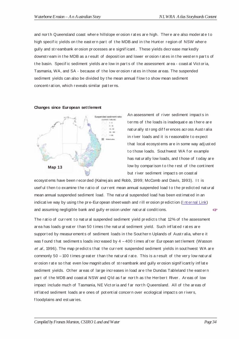
Waterborne Erosion – An Australian Story NLWRA Atlas Storyboards Content
Compiled by Frances Marston, CSIRO Land and Water Page 34
and north Queensland coast where hillslope erosion rates are high. There are also moderate to
high specific yields on the eastern part of the MDB and in the Hunter region of NSW where
gully and streambank erosion processes are significant. These yields decrease markedly
downstream in the MDB as a result of deposition and lower erosion rates in the western parts of
the basin. Specific sediment yields are low in parts of the assessment area - coastal Victoria,
Tasmania, WA, and SA - because of the low erosion rates in those areas. The suspended
sediment yields can also be divided by the mean annual flow to show mean sediment
concentration, which reveals similar patterns.
Changes since European settlement
An assessment of river sediment impacts in
terms of the loads is inadequate as there are
naturally strong differences across Australia
in river loads and it is reasonable to expect
that local ecosystems are in some way adjusted
to those loads. Southwest WA for example
has naturally low loads, and those of today are
low by comparison to the rest of the continent
but river sediment impacts on coastal
ecosystems have been recorded (Kalnejais and Robb, 1999; McComb and Davis, 1993). It is
useful then to examine the ratio of current mean annual suspended load to the predicted natural
mean annual suspended sediment load. The natural suspended load has been estimated in an
indicative way by using the pre-European sheetwash and rill erosion prediction (Internal Link)
and assuming negligible bank and gully erosion under natural conditions. ☞
The ratio of current to natural suspended sediment yield predicts that 12% of the assessment
area has loads greater than 50 times the natural sediment yield. Such inflated rates are
supported by measurements of sediment loads in the Southern Uplands of Australia, where it
was found that sediments loads increased by 4 – 400 times after European settlement (Wasson
et al., 1996). The map predicts that the current suspended sediment yields in southwest WA are
commonly 50 – 100 times greater than the natural rate. This is a result of the very low natural
erosion rate so that even low magnitudes of streambank and gully erosion significantly inflate
sediment yields. Other areas of large increases in load are the Dundas Tableland the eastern
part of the MDB and coastal NSW and Qld as far north as the Herbert River. Areas of low
impact include much of Tasmania, NE Victoria and far north Queensland. All of the areas of
inflated sediment loads are ones of potential concern over ecological impacts on rivers,
floodplains and estuaries.
Map 13
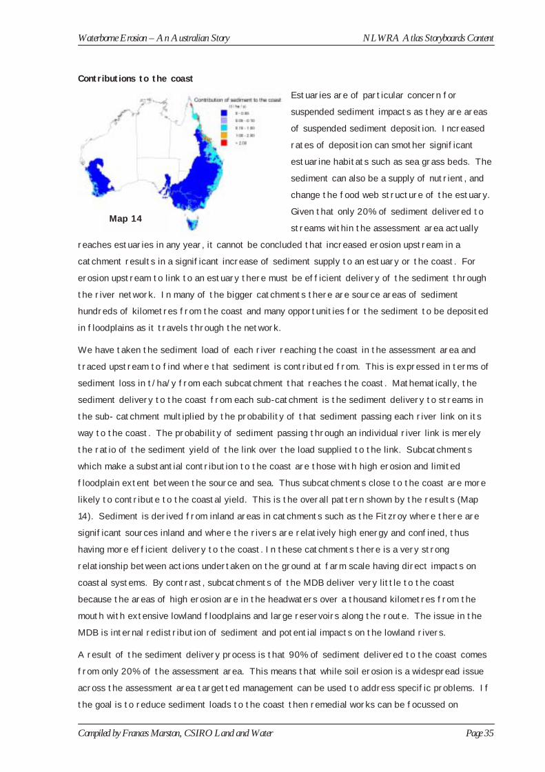
Waterborne Erosion – An Australian Story NLWRA Atlas Storyboards Content
Compiled by Frances Marston, CSIRO Land and Water Page 35
Contributions to the coast
Estuaries are of particular concern for
suspended sediment impacts as they are areas
of suspended sediment deposition. Increased
rates of deposition can smother significant
estuarine habitats such as sea grass beds. The
sediment can also be a supply of nutrient, and
change the food web structure of the estuary.
Given that only 20% of sediment delivered to
streams within the assessment area actually
reaches estuaries in any year, it cannot be concluded that increased erosion upstream in a
catchment results in a significant increase of sediment supply to an estuary or the coast. For
erosion upstream to link to an estuary there must be efficient delivery of the sediment through
the river network. In many of the bigger catchments there are source areas of sediment
hundreds of kilometres from the coast and many opportunities for the sediment to be deposited
in floodplains as it travels through the network.
We have taken the sediment load of each river reaching the coast in the assessment area and
traced upstream to find where that sediment is contributed from. This is expressed in terms of
sediment loss in t/ha/y from each subcatchment that reaches the coast. Mathematically, the
sediment delivery to the coast from each sub-catchment is the sediment delivery to streams in
the sub- catchment multiplied by the probability of that sediment passing each river link on its
way to the coast. The probability of sediment passing through an individual river link is merely
the ratio of the sediment yield of the link over the load supplied to the link. Subcatchments
which make a substantial contribution to the coast are those with high erosion and limited
floodplain extent between the source and sea. Thus subcatchments close to the coast are more
likely to contribute to the coastal yield. This is the overall pattern shown by the results (Map
14). Sediment is derived from inland areas in catchments such as the Fitzroy where there are
significant sources inland and where the rivers are relatively high energy and confined, thus
having more efficient delivery to the coast. In these catchments there is a very strong
relationship between actions undertaken on the ground at farm scale having direct impacts on
coastal systems. By contrast, subcatchments of the MDB deliver very little to the coast
because the areas of high erosion are in the headwaters over a thousand kilometres from the
mouth with extensive lowland floodplains and large reservoirs along the route. The issue in the
MDB is internal redistribution of sediment and potential impacts on the lowland rivers.
A result of the sediment delivery process is that 90% of sediment delivered to the coast comes
from only 20% of the assessment area. This means that while soil erosion is a widespread issue
across the assessment area targetted management can be used to address specific problems. If
the goal is to reduce sediment loads to the coast then remedial works can be focussed on
Map 14

Waterborne Erosion – An Australian Story NLWRA Atlas Storyboards Content
Compiled by Frances Marston, CSIRO Land and Water Page 36
particular sediment sources and the land uses and erosion processes found there. Relatively
little attention is needed for the rest of the catchment. Sediment delivery to the coast is not
the only concern and the same principles can be applied if the target is to reduce sediment
delivery to particular reservoirs, lakes or individual river reaches of high value.
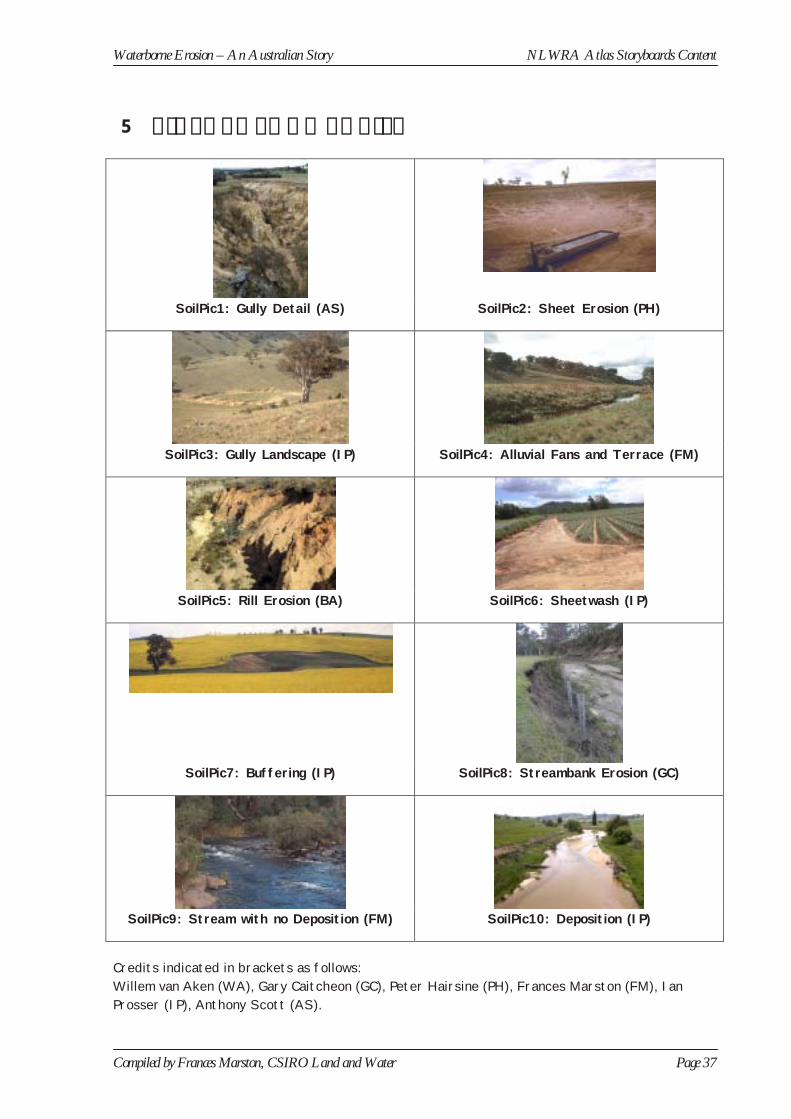
Waterborne Erosion – An Australian Story NLWRA Atlas Storyboards Content
Compiled by Frances Marston, CSIRO Land and Water Page 37
5 PICTURE THUMBNAILS
SoilPic1: Gully Detail (AS) SoilPic2: Sheet Erosion (PH)
SoilPic3: Gully Landscape (IP) SoilPic4: Alluvial Fans and Terrace (FM)
SoilPic5: Rill Erosion (BA) SoilPic6: Sheetwash (IP)
SoilPic7: Buffering (IP) SoilPic8: Streambank Erosion (GC)
SoilPic9: Stream with no Deposition (FM) SoilPic10: Deposition (IP)
Credits indicated in brackets as follows: Willem van Aken (WA), Gary Caitcheon (GC), Peter Hairsine (PH), Frances Marston (FM), Ian Prosser (IP), Anthony Scott (AS).

Waterborne Erosion – An Australian Story NLWRA Atlas Storyboards Content
Compiled by Frances Marston, CSIRO Land and Water Page 38
6 REFERENCES
Abernethy, B. and Rutherfurd, I.D. (2000). The effect of riparian tree roots on riverbank
stability. Earth Surface Processes and Landforms 25:921-37.
Brooks, A. (1999). Lessons for river managers from the fluvial tardis. In Second Australian Stream Management Conference: The Challenge of Rehabilitating Australia’s Streams,
Rutherfurd, I.D. and R. Bartley (Eds.), pp. 121-8. Cooperative Research Centre for Catchment
Hydrology: Melbourne.
Brune, G.M. (1953). Trap efficiency of reservoirs. Transactions, American Geophysical Union, 34(3): 407-418.
Edwards, K. (1993). Soil erosion and conservation in Australia. In World Soil Erosion and Conservation. Pimental, D. (Ed.) pp 147-69. (Cambridge University Press: Cambridge.)
Erskine, W and Bell, F.C. (1982). Rainfall, floods and river channel changes in the upper
Hunter. Australin Geographical Studies 20:183-195
Ford, G.W., Martin, J.J., Rengasamy, P., Boucher, S.C., and Ellington, A. (1993). Soil
sodicity in Victoria. Australian Journal of Soil Research 31:869-909.
Graham, O.P. (1989). Land degradation survey of NSW 1987-88: Methodology. SCS Technical
Report No. 7. Soil Conservation Service of NSW.
Kalnejais, L. and Robb, M. (1999). Water quality in Wilson Inlet 1995-1997: a resport on the
monitoring data collected between 1995 and 1997. Report (Western Australia, Water and Rivers Commission), no. WRT14, 61p.
Littleboy, M., Silburn, D.M., Freebairn, D.M., Woodruff, D.R., Hammer, G.L., and
Leslie, J.K. (1992). Impact of soil erosion on production in cropping systems. I. Development
and validation of a simulation model. Australian Journal of Soil Research, 30(5):757-774.
Loch, R. J., B. K. Slater, B. K. and Devoil, C. (1998). Soil erodibility (Km) values for some Australian soils. Aust. J. Soil Res., 36, 1045-55. McComb,A.J. and Davis, J.A. (1993). Eutrophic waters of southwestern Australia. Fertilizer Research, 36(2):105-114.
McCool, D.K., Foster, G.R., Mutchler, C.K., and Meyer, L.D. (1989). Revised slope length
factor in the Universal Soil Loss Equation. Transactions of the American Society of Agricultural Engineers, 32(5):1571-1576.
Moore, I.D. and Burch, G.J. (1986). Physical basis for the length-slope factor in the universal
soil loss equation. Soil Science Society of America Journal 50:1294-1298.

Waterborne Erosion – An Australian Story NLWRA Atlas Storyboards Content
Compiled by Frances Marston, CSIRO Land and Water Page 39
Prosser, I. P. and Winchester, S.J. (1996). History and processes of gully initiation and
development in Australia. Zeitschrift Fur Geomorphologie Suppl.-Bd 105:91-109.
Prosser, I., Rutherfurd, I.D., Olley, J.M., Young, W.J., Wallbrink, P.J. and Moran, C.J.
(2001). Large-scale patterns of erosion and sediment transport in river networks, with examples
from Australia. Marine and Freshwater Research 52:81-99.
Renard, K.G., Foster, G.A., Weesies, D.K., McCool, D.K., and Yoder, D.C. (1997).
Predicting soil erosion by water: A guide to conservation planning with the revised universal soil
loss equation. Agriculture Handbook 703, United States Department of Agriculture, Washington
DC.
Rosewell, C.J. (1993). SOILOSS - A program to assist in the selection of management
practices to reduce erosion. Technical Handbook No. 11 (2nd edition), Soil Conservation Service
of NSW, Sydney.
Rutherford, I. (2000). Some human impacts on Australian stream channel morphology. In River Management: The Australasian Experience, Brizga, S. and Finlayson, B. (Eds), John Wiley and
Sons Ltd.
Sharman, P.E.V. and Murphy, B.W. (1991). Soils their properties and management: a soil
conservation handbook for New South Wales. Sydney University Press in association with
Oxford University Press, Australia and Soil Conservation Service of New South Wales.
Wasson, R.J., Mazari, R.K., Starr, B. and Clifton, G. (1998). The recent history of erosion
and sedimentation on the Southern Tablelands of southeastern Australia: sediment flux
dominated by channel incision. Geomorphology 24:291-308.
Wasson, R.J., Olive, L. J., and Rosewell, C. J. (1996). Rates of erosion and sediment
transport in Australia. Erosion and Sediment Yield: Global and Regional Perspectives. IAHS Publ.
No. 236: 139-148.
Whittow, J. (1986). Dictionary of physical geography. Penguin Books, Middlesex, England.
Wischmeier, W. H. and Smith, D. D. (1978). Predicting rainfall erosion losses: A guide to
conservation planning. US Department of Agriculture. Agriculture Handbook No. 537. (US
Government Printing Office: Washington, DC).

Waterborne Erosion – An Australian Story NLWRA Atlas Storyboards Content
Compiled by Frances Marston, CSIRO Land and Water Page 40
7 APPENDIX: RIVER BASIN ANALYSIS
This section presents summary statistics in the context of the AWRC basin definitions, ie with
reference to standard basin names and numbers.
EACH TABLE ITEM (COLUMN) IS DESCRIBED AS FOLLOWS:
Basin Name: as defined by the AWRC.
Basin No.: as defined by the AWRC.
Area (km2): the area in km2 of each basin as derived from the DEM.
Sediment supply (t/ha/y) : This is the total sediment supplied to streams on an annual basis
from the following sediment sources; hillslope erosion, bank erosion and gully erosion. The
contribution from each source is summed in tonnes per year for each basin and then divided by
the total area in hectares of each basin to give sediment supply in t/ha/y.
Proportion from hillslopes and bank erosion and percentage from gullies: This is calculated
for each basin by dividing the sum of each component (t/y) by the total sediment supply value
for each basin (t/y).
Proportion of length with bed deposition greater than 0.30 m. This is calculated by summing
the stream length in each basin with deposition greater than 0.30 m then dividing by the total
stream length in each basin.
Sediment Ratio (Euro/Pre-European). This is the average ratio of item 2 under present land use conditions to that of item 2 under natural conditions for each river basin.
Sediment export to the coast (t/y). This is the mean annual amount of sediment delivered by
each basin to the coast in tonnes per year. It is has been summed for each basin.
Specific sediment export to the coast (t/ha/y). This is the above item divided by the area in
hectares for each basin.
River sediment delivery ratio (export/supply to streams). This is item 6 for each basin
divided by item 2 in t/y.
POINTS TO NOTE ABOUT THE ACCURACY OF THE MODEL OUTPUTS.
1. All but one of the MDB catchments do not export directly to the coast. The figures for
individual MDB basins (no’s 401 – 425) in items 6 , 7 and 8 are therefore the contribution
of each basin to the MDB total export to the coast, which is made by basin number 426.
2. The model ouputs for the lowland MDB catchments have been derived from low quality
data, which primarily results from the physical properties of the rivers and the
somewhat arbitrary AWRC basin boundaries.

Waterborne Erosion – An Australian Story NLWRA Atlas Storyboards Content
Compiled by Frances Marston, CSIRO Land and Water Page 41
Summary statistics for river basin analysesBasin Name Basin
No.
Area
(km2)
Sediment
supply(t/ha/y)
Proportion
fromhillslopes
(%)
Proportion
from bankerosion
(%)
% from
gullies
Prop. of
lengthwith beddeposn.
> 0.30m
Sed
Ratio(Euro/pre-
Euro)
Sediment
export to thecoast(t/y)
Specific
sedimentexport to thecoast (t/ha/y)
River sed.
delivery ratio(export/supply
to streams)
Jacky Jacky Creek 101 1,731 2.5 85 11 4 0.00 52 329,832 1.9 0.77
Olive / Pascoe Rivers 102 3,849 2.6 79 18 3 0.00 46 712,764 1.9 0.71
Lockhart River 103 2,008 0.4 22 77 0 0.00 23 37,137 0.2 0.49
Stewart River 104 2,346 1.4 70 24 7 0.05 10 160,798 0.7 0.51
Normanby River 105 24,440 1.6 88 3 9 0.02 3 1,620,279 0.7 0.42
Jeannie River 106 2,589 1.9 94 4 2 0.00 3 355,885 1.4 0.71
Endeavour River 107 1,951 3.1 97 2 1 0.00 5 486,871 2.5 0.80
Daintree River 108 1,548 0.7 82 17 1 0.00 4 94,132 0.6 0.84
Mossman River 109 318 0.6 78 21 2 0.00 5 15,131 0.5 0.80
Barron River 110 2,151 1.2 79 10 10 0.00 8 145,877 0.7 0.57
Mulgrave-Russell River 111 1,664 1.7 70 28 2 0.04 6 222,425 1.3 0.78
Johnstone River 112 2,240 1.7 65 29 6 0.00 29 305,142 1.4 0.78
Tully River 113 1,743 0.9 33 63 5 0.00 6 88,084 0.5 0.59
Murray River 114 716 0.5 27 65 8 0.00 6 17,098 0.2 0.53
Herbert River 116 9,605 1.4 75 12 14 0.08 8 664,787 0.7 0.51
Black River 117 705 1.7 92 4 4 0.01 3 82,887 1.2 0.69
Ross River 118 1,143 1.8 88 4 8 0.00 2 58,383 0.5 0.28
Haughton River 119 3,763 1.9 81 5 13 0.13 10 172,454 0.5 0.25
Burdekin River 120 129,454 1.4 67 6 27 0.11 15 2,443,232 0.2 0.13
Don River 121 3,018 3.1 86 3 11 0.04 11 509,528 1.7 0.55
Proserpine River 122 1,847 2.0 88 7 5 0.07 31 227,314 1.2 0.63
O'Connell River 124 1,980 2.4 89 8 4 0.06 45 366,309 1.9 0.77
Pioneer River 125 1,689 2.3 86 10 4 0.00 28 288,343 1.7 0.73
Plane Creek 126 1,534 1.1 78 13 9 0.00 46 114,860 0.7 0.67
Styx River 127 2,510 1.2 78 8 14 0.09 31 136,011 0.5 0.44
Shoalwater Creek 128 2,664 0.5 57 18 25 0.19 12 45,166 0.2 0.37
Water Park Creek 129 562 0.2 65 14 21 0.00 27 7,940 0.1 0.67
Fitzroy River 130 142,831 1.1 63 13 25 0.19 21 2,635,482 0.2 0.16
Calliope River 132 1,947 0.8 50 16 34 0.15 35 60,772 0.3 0.37
Boyne River 133 2,488 0.4 31 37 33 0.00 8 16,974 0.1 0.16
Baffle Creek 134 3,390 0.6 64 15 21 0.04 29 103,376 0.3 0.50
Kolan River 135 2,796 0.7 55 19 26 0.11 36 61,589 0.2 0.30
Burnett River 136 33,741 0.9 44 24 32 0.15 96 728,607 0.2 0.25

Waterborne Erosion – An Australian Story NLWRA Atlas Storyboards Content
Compiled by Frances Marston, CSIRO Land and Water Page 42
Summary statistics for river basin analysesBasin Name Basin
No.
Area
(km2)
Sediment
supply(t/ha/y)
Proportion
fromhillslopes
(%)
Proportion
from bankerosion
(%)
% from
gullies
Prop. of
lengthwith beddeposn.
> 0.30m
Sed
Ratio(Euro/pre-
Euro)
Sediment
export to thecoast(t/y)
Specific
sedimentexport to thecoast (t/ha/y)
River sed.
delivery ratio(export/supply
to streams)
Burrum River 137 2,931 0.3 53 27 20 0.00 36 33,624 0.1 0.40
Mary River 138 9,398 0.7 39 44 17 0.11 18 266,713 0.3 0.40
Noosa River 140 1,227 0.2 10 52 38 0.04 15 7,288 0.1 0.39
Maroochy River 141 1,077 0.7 52 29 19 0.00 28 45,525 0.4 0.57
Pine River 142 1,258 0.5 45 34 21 0.00 40 20,687 0.2 0.35
Brisbane River 143 13,602 0.9 54 26 20 0.07 37 247,194 0.2 0.19
Logan-Albert River 145 4,045 1.2 58 25 18 0.19 35 189,138 0.5 0.40
South Coast 146 1,104 0.4 21 54 25 0.00 10 20,641 0.2 0.44
Tweed River 201 1,055 0.9 53 41 6 0.25 16 58,498 0.6 0.64
Brunswick River 202 133 0.2 49 35 16 0.00 5 2,158 0.2 0.68
Richmond River 203 6,760 0.8 42 41 17 0.13 32 240,825 0.4 0.43
Clarence River 204 22,084 0.8 25 44 32 0.07 198 683,379 0.3 0.40
Bellinger River 205 3,082 0.5 7 65 28 0.08 101 61,591 0.2 0.43
Macleay River 206 11,395 0.9 30 29 41 0.13 65 345,455 0.3 0.34
Hastings River 207 4,209 0.5 7 70 24 0.09 332 83,255 0.2 0.44
Manning River 208 7,939 0.7 15 47 39 0.03 56 224,159 0.3 0.42
Karuah River 209 3,665 0.5 16 40 44 0.15 161 72,363 0.2 0.41
Hunter River 210 21,138 1.4 33 20 46 0.33 630 743,606 0.4 0.25
Macquarie - Tuggerah Lakes 211 1,384 0.3 11 30 59 0.32 111 13,915 0.1 0.37
Hawkesbury River 212 21,636 0.5 21 28 50 0.08 211 233,011 0.1 0.21
Sydney Coast - Georges R. 213 1,511 0.2 7 53 40 0.09 323 11,226 0.1 0.30
Wollongong Coast 214 490 0.4 12 21 67 0.00 3 8,904 0.2 0.42
Shoalhaven River 215 7,172 0.6 14 26 60 0.10 27 135,530 0.2 0.33
Clyde River - Jervis Bay 216 2,666 0.3 5 28 68 0.18 20 34,173 0.1 0.39
Moruya River 217 1,505 0.4 14 19 66 0.10 44 24,362 0.2 0.40
Tuross River 218 1,902 0.4 7 22 72 0.13 41 23,959 0.1 0.34
Bega River 219 2,507 0.5 9 31 61 0.12 191 40,908 0.2 0.33
Towamba River 220 1,708 0.4 4 29 66 0.04 48 26,302 0.2 0.39
East Gippsland 221 5,103 0.1 6 47 47 0.01 36 25,818 0.1 0.40
Snowy River 222 15,360 0.5 21 26 53 0.04 16 303,309 0.2 0.37
Tambo River 223 4,249 0.1 9 59 32 0.02 19 18,114 0.0 0.30
Mitchell River 224 4,749 0.1 11 85 3 0.02 3 25,330 0.1 0.36
Thomson River 225 6,443 0.2 6 81 13 0.01 108 23,583 0.0 0.21

Waterborne Erosion – An Australian Story NLWRA Atlas Storyboards Content
Compiled by Frances Marston, CSIRO Land and Water Page 43
Summary statistics for river basin analysesBasin Name Basin
No.
Area
(km2)
Sediment
supply(t/ha/y)
Proportion
fromhillslopes
(%)
Proportion
from bankerosion
(%)
% from
gullies
Prop. of
lengthwith beddeposn.
> 0.30m
Sed
Ratio(Euro/pre-
Euro)
Sediment
export to thecoast(t/y)
Specific
sedimentexport to thecoast (t/ha/y)
River sed.
delivery ratio(export/supply
to streams)
Latrobe River 226 5,102 0.2 6 92 2 0.08 5 31,953 0.1 0.26
South Gippsland 227 4,680 0.2 15 85 0 0.01 15 41,644 0.1 0.40
Bunyip River 228 2,714 0.2 6 83 11 0.00 >1,000 21,882 0.1 0.34
Yarra River 229 4,092 0.3 3 78 19 0.00 7 37,091 0.1 0.28
Maribyrnong River 230 1,432 0.5 8 57 35 0.00 10 26,644 0.2 0.36
Werribee River 231 1,847 0.3 23 46 31 0.01 9 8,885 0.0 0.17
Moorabool River 232 1,964 0.4 12 39 48 0.04 70 16,766 0.1 0.23
Barwon River 233 3,276 0.3 7 59 33 0.13 35 23,601 0.1 0.21
Lake Corangamite 234 2,038 0.3 8 40 52 0.12 53 0 0.0 0.00
Otway Coast 235 3,024 0.2 11 82 6 0.09 16 22,950 0.1 0.42
Hopkins River 236 8,902 0.5 3 44 53 0.22 198 64,382 0.1 0.14
Portland Coast 237 3,532 0.2 4 79 17 0.04 >1,000 19,143 0.1 0.30
Glenelg River 238 11,622 0.6 2 30 68 0.38 309 147,721 0.1 0.21
Millicent Coast 239 3,583 0.2 4 82 15 0.06 77 0 0.0 0.00
East Coast 302 4,351 0.2 24 35 40 0.01 5 44,400 0.1 0.51
Coal River 303 580 0.6 34 23 43 0.09 11 15,544 0.3 0.48
Derwent River 304 9,556 0.4 13 65 22 0.03 47 149,437 0.2 0.43
Kingston Coast 305 117 0.1 32 36 32 0.00 3 727 0.1 0.66
Huon River 306 2,964 0.4 7 82 11 0.00 16 57,413 0.2 0.51
South-West Coast 307 3,531 0.5 5 95 0 0.03 9 99,086 0.3 0.51
Gordon River 308 5,311 0.5 2 95 3 0.00 186 127,593 0.2 0.46
King-Henty Rivers 309 1,620 0.1 24 76 0 0.00 96 4,903 0.0 0.59
Pieman River 310 3,899 0.1 12 86 2 0.00 138 16,698 0.0 0.45
Sandy Cape Coast 311 180 0.3 1 99 0 0.00 102 2,712 0.2 0.49
Arthur River 312 2,475 0.2 4 94 2 0.00 36 19,726 0.1 0.51
Smithton-Burnie Coast 314 3,362 0.2 6 86 8 0.00 27 34,941 0.1 0.49
Forth River 315 1,110 0.2 12 49 38 0.00 1 6,339 0.1 0.37
Mersey River 316 1,898 0.6 6 56 38 0.00 6 51,007 0.3 0.48
Rubicon River 317 443 0.3 3 37 61 0.00 12 7,020 0.2 0.47
Tamar River 318 11,068 0.4 9 70 21 0.07 6 195,373 0.2 0.42
Piper-Ringarooma Rivers 319 3,029 0.3 5 49 47 0.00 7 39,746 0.1 0.46
Upper Murray River 401 16,177 0.4 23 45 32 0.03 8 2,783 0.0 0.00
Kiewa River 402 1,924 0.6 13 62 25 0.00 3 4,582 0.0 0.04

Waterborne Erosion – An Australian Story NLWRA Atlas Storyboards Content
Compiled by Frances Marston, CSIRO Land and Water Page 44
Summary statistics for river basin analysesBasin Name Basin
No.
Area
(km2)
Sediment
supply(t/ha/y)
Proportion
fromhillslopes
(%)
Proportion
from bankerosion
(%)
% from
gullies
Prop. of
lengthwith beddeposn.
> 0.30m
Sed
Ratio(Euro/pre-
Euro)
Sediment
export to thecoast(t/y)
Specific
sedimentexport to thecoast (t/ha/y)
River sed.
delivery ratio(export/supply
to streams)
Ovens River 403 8,083 0.5 10 50 40 0.09 24 15,788 0.0 0.04
Broken River 404 4,795 0.5 6 45 49 0.22 17 6,635 0.0 0.03
Goulburn River 405 16,133 0.6 8 45 47 0.19 11 46,712 0.0 0.05
Campaspe River 406 3,980 1.1 3 18 80 0.52 23 10,690 0.0 0.02
Loddon River 407 11,937 0.7 3 25 72 0.47 44 4,459 0.0 0.01
Avoca River 408 5,956 0.8 4 16 80 0.55 40 0 0.0 0.00
Murray-Riverina 409 10,552 1.0 1 88 10 0.25 103 101,001 0.1 0.09
Murrumbidgee River 410 63,011 0.7 12 36 51 0.34 434 109,163 0.0 0.02
Lake George 411 275 0.9 27 7 66 0.94 29 0 0.0 0.00
Lachlan River 412 63,497 0.7 14 30 56 0.30 22 21,627 0.0 0.00
Benanee 413 3,146 1.4 1 99 0 0.27 9 95,127 0.3 0.21
Wimmera - Avon Rivers 415 9,839 0.7 4 24 72 0.47 63 0 0.0 0.00
Border Rivers 416 43,133 1.1 19 23 59 0.47 268 1,548 0.0 0.00
Moonie River 417 9,685 0.3 25 48 28 0.22 22 1 0.0 0.00
Gwydir River 418 21,812 1.4 21 24 55 0.34 45 1,415 0.0 0.00
Namoi River 419 38,373 1.3 28 25 47 0.32 74 1,671 0.0 0.00
Castlereagh River 420 14,430 0.7 17 43 40 0.33 220 178 0.0 0.00
Macquarie-Bogan Rivers 421 67,927 0.8 21 43 36 0.25 107 1,109 0.0 0.00
Condamine-Culgoa Rivers 422 102,723 0.5 28 34 38 0.28 34 231 0.0 0.00
Warrego River 423 44,649 0.4 43 37 20 0.17 16 91 0.0 0.00
Paroo River 424 39,906 0.3 47 40 13 0.09 13 0 0.0 0.00
Darling River 425 50,853 0.7 9 81 10 0.25 24 169,797 0.0 0.05
Lower Murray River 426 24,229 0.8 13 75 12 0.41 14 564,300 0.2 0.27
Fleurieu Peninsula 501 409 0.9 3 8 90 0.00 12 13,310 0.3 0.38
Myponga River 502 132 0.1 45 31 24 0.00 1 641 0.0 0.43
Onkaparinga River 503 679 0.2 16 50 35 0.00 4 3,820 0.1 0.31
Torrens River 504 890 0.2 15 68 18 0.00 2 3,223 0.0 0.24
Gawler River 505 4,300 0.3 12 43 45 0.18 11 25,422 0.1 0.22
Wakefield River 506 1,397 0.3 13 30 57 0.15 10 5,466 0.0 0.12
Broughton River 507 11,931 0.3 16 29 55 0.11 9 56,140 0.0 0.16
Mambray Coast 508 4,485 0.2 49 9 42 0.07 29 29,033 0.1 0.26
Willochra Creek 509 6,001 0.4 20 18 63 0.48 13 0 0.0 0.00
Lake Torrens 510 14,113 0.4 48 8 44 0.32 13 1,434 0.0 0.00

Waterborne Erosion – An Australian Story NLWRA Atlas Storyboards Content
Compiled by Frances Marston, CSIRO Land and Water Page 45
Summary statistics for river basin analysesBasin Name Basin
No.
Area
(km2)
Sediment
supply(t/ha/y)
Proportion
fromhillslopes
(%)
Proportion
from bankerosion
(%)
% from
gullies
Prop. of
lengthwith beddeposn.
> 0.30m
Sed
Ratio(Euro/pre-
Euro)
Sediment
export to thecoast(t/y)
Specific
sedimentexport to thecoast (t/ha/y)
River sed.
delivery ratio(export/supply
to streams)
Spencer Gulf 511 8,069 0.1 47 27 26 0.01 37 21,507 0.0 0.20
Eyre Peninsula 512 1,720 0.1 12 70 18 0.03 3 3,373 0.0 0.30
Kangaroo Island 513 3,039 0.2 3 27 70 0.01 63 17,111 0.1 0.34
Esperance Coast 601 14,683 0.2 7 19 75 0.07 259 40,274 0.0 0.15
Albany Coast 602 16,765 0.3 6 20 75 0.22 76 80,131 0.0 0.19
Denmark River 603 2,582 0.4 1 17 82 0.09 36 31,091 0.1 0.32
Kent River 604 2,376 0.2 1 18 81 0.11 426 14,816 0.1 0.27
Frankland River 605 4,686 0.4 1 16 83 0.57 92 26,392 0.1 0.14
Shannon River 606 2,450 0.1 1 39 61 0.00 170 5,264 0.0 0.41
Warren River 607 4,404 0.2 1 32 67 0.08 80 27,922 0.1 0.25
Donnelly River 608 1,714 0.1 1 30 69 0.01 57 5,886 0.0 0.37
Blackwood River 609 22,970 0.3 3 27 70 0.37 247 97,576 0.0 0.12
Busselton Coast 610 2,315 0.3 3 35 62 0.05 817 24,238 0.1 0.34
Preston River 611 1,168 0.6 2 33 65 0.00 29 24,565 0.2 0.34
Collie River 612 3,698 0.3 3 39 58 0.11 >1,000 21,630 0.1 0.21
Harvey River 613 1,460 0.4 3 45 52 0.11 106 17,138 0.1 0.31
Murray River (WA) 614 9,583 0.5 2 23 75 0.55 598 84,754 0.1 0.18
Avon River 615 42,881 0.4 4 20 76 0.60 470 75,636 0.0 0.05
Swan Coast 616 7,239 0.5 2 24 74 0.32 418 89,746 0.1 0.24
Moore-Hill Rivers 617 11,535 0.5 3 16 82 0.54 32 50,819 0.0 0.10
Yarra Yarra Lakes 618 6,125 0.2 17 14 69 0.10 229 0 0.0 0.00
Ninghan 619 976 0.2 22 21 58 0.00 415 0 0.0 0.00
Greenough River 701 18,076 0.4 6 18 76 0.45 91 116,012 0.1 0.16
Murchison River 702 50,658 0.3 25 21 54 0.14 9 21,096 0.0 0.01
Minimum 117 0.1 1 2 0 0.00 1 0 0.0 0.0
Median 3,531 0.5 14 30 32 0.07 29 30,062 0.1 0.3
Maximum 142,831 3.1 97 99 90 0.94 817 2,635,482 2.5 0.8
Total 1,667,300 21,139,700