wave-equation migration velocity analysis using partial

Wave-equation migration velocity analysis using

partial-stack power maximization

Yang Zhang and Guojian Shan

ABSTRACT

We proposed to use a partial-stack power maximization objective function inwave-equation migration velocity analysis. Instead of stacking the angle-domaincommon-image gathers all at once, the partial-stack power maximization objec-tive function stacks them in smaller groups. It improves the robustness againstthe cycle-skipping problem and can achieve better global convergence. We alsoadded a normalization term to the partial-stack power maximization objectivefunction to balance the different reflector amplitudes. We tested our objectivefunction using the Marmousi model. The results demonstrate that using thepartial-stack power maximization criterion can achieve better global convergence.We also observed that the normalization of reflector amplitudes is very importantin order to better constrain the tomography problem.

INTRODUCTION

Introduced by Gardner (1974) and Sattlegger (1975), migration velocity analysis(MVA) belongs to a family of methods for estimation of migration velocity. Insteadof looking at travel-times in the seismic data, MVA extracts the velocity informationfrom the migrated images. Etgen (1990) and van Trier (1990) proposed the first for-mulations of tomographic MVA using surface offset-domain common-image-gathers(ODCIGs) obtained by Kirchhoff migration. Recently, the tomographic MVA methodhas been extended to wave-equation migration velocity analysis (WEMVA), whichuses the wave-equation rather than the ray-based model to resolve the velocity infor-mation (Chavent and Jacewitz, 1995; Biondi and Sava, 1999). The wave-equation-based methods are more accurate than ray-based methods, because the wave-equationbetter describes wave-propagation physics and provides physically more realistic sen-sitivity kernels for the velocity update. The wave-equation model can behave quitedifferently than the ray-based model when applied to complex velocity models.

To estimate velocity, WEMVA solves an optimization problem. Evaluating theflatness of the subsurface angle-domain common-image gathers (ADCIGs) is currentlya popular choice when forming WEMVA objective functions (Biondi and Sava, 1999;Clapp and Biondi, 2000; Biondi and Symes, 2004). The objective function is usuallyoptimized by applying gradient-based algorithms. The computation of the gradientis performed in two steps: 1) computation of a perturbation in the migrated image

SEP–149

Zhang and Shan 2 Partial-stack power maximization

domain, and 2) back-projection of the image perturbation into the velocity model us-ing the image-space wave-equation tomographic (ISWET) operator (Sava and Biondi,2004).

Several ADCIGs-based WEMVA objective functions have been proposed in theliterature. The stack power maximization (SPM) method directly maximizes thestack of the ADCIGs of all detectable angles, but similar to full-waveform inversion(FWI) (Tarantola, 1984), it is prone to cycle-skipping when the starting model isnot sufficiently accurate and the data do not contain very low frequencies (Symes,2008). Differential-semblance optimization (DSO) (Symes and Carazzone, 1991; Shenet al., 2005; Shen and Symes, 2008) penalizes the difference between the ADCIGs ofneighboring angles (or the unfocused energy on the subsurface ODCIGs). This objec-tive function can achieve much better global convergence. However, the differencingoperator amplifies the high-frequency (with respect to the angle axis) image varia-tions in the ADCIGs and can generate unwanted artifacts in the gradient (Fei andWilliamson, 2010), which slows down convergence.

If we compare the two objective functions that previously mentioned, notice that“stacking all angles” is a special case of the smoothing operations, and it extractsnothing but the zero-frequency component (with regard to the angle axis), while “dif-ferencing neighboring angles” extracts all frequency components but boosts higher-frequency components. The partial-stack power maximization objective function isa compromise between the two. It utilizes many non-zero frequency components asDSO does, while still using the stacking operator (in contrast to the differencing op-erator) with smaller windows. Having higher-frequency components in the objectivefunctions ensures better global convergence, and not using the differencing operatoravoids amplifying the high-frequency noise in the ADCIGs. Therefore the partial-stack power maximization objective function combines the merits of the SPM andDSO objective functions.

The rest of this paper is divided into two parts: first we present the mathematicalformulation; then we demonstrate the effectiveness of our method with the Marmousiexamples.

THEORY

Partial-Stack power maximization

For the sake of simplicity, we assume two-dimensions in our derivation; however, ex-tending the theory to 3-D is straightforward for this method. We denote the prestackimage as I(z, γ, x), (x, z are the depth and horizontal axis, and γ is the reflection-aperture angle).

To enforce the goal of ADCIG flatness, we have multiple options in choosing theobjective functions. The stack power maximization (Soubaras and Gratacos, 2007)

SEP–149


maximizes the full angle stack of the ADCIG:

maxv

JSPM(v) =1

2‖∑

γ

I(z, x, γ; v)‖22, (1)

in which I(z, x, γ; v) is the ADCIGs migrated using the current velocity model v. Thisapproach can yield a high-resolution model, however when the velocity error is large,the angle gathers will become strongly curved and demonstrate significant residualmoveout (RMO) (different amounts of event shifts at different angles). Because westack all angles at once, as the difference of event shifts between angles becomes biggerthan half wavelength of the dominant frequency, the stacking becomes incoherent andwould result in two separate events instead of one. The cycle-skipping phenomenonarises from such situations.

As another option to enforce angle-gather flatness, the differential semblance op-timization (DSO) objective function proposed by Shen et al. (2005) overcomes thiscycle-skipping issue by using a local operator that operates on each individual angleand its immediate neighbors:

minv

JDSO(v) =1

2‖∂I(z, x, γ; v)

∂γ‖2

2. (2)

Cycle-skipping is very unlikely to happen using the DSO objective function, becausethe relative shifts in the gathers between one angle and its neighbors is generally verysmall.

However, the differencing operator is poorly conditioned (i.e., the operator is veryshort, spanning over only two angles and therefore requires many iterations to makeall angles the same), and it magnifies the high-frequency variations of the ADCIGsalong the axis of reflection angle. In several cases these high-frequency variationsare not desired (for example, when high-frequency noise is present in ADCIGs, orwhen the variations are caused mainly by non-uniform subsurface illumination ateach reflection angle).

In order to combine the advantages of both approaches, Shen and Symes (2008)introduce a bi-objective function that includes both terms using the weighted sum:

minv

JCMB(v) = JDSO(v) − βJSPM(v). (3)

As expected, this approach can achieve both global and local convergence, but thedisadvantage brought by the differencing operator still remains, and adjusting theparameter β (β ≥ 0) might not be trivial.

The partial-stack power maximization (partial SPM) objective function is an al-ternative way to combine the SPM and DSO objective functions. We use a partiallystacking operator that has a span between those of the full stacking operator and thedifferencing operator:

maxv

JPSPM(v) =1

2‖∑

γ

{g(γ) ∗ I(z, x, γ; v)}‖22, (4)

SEP–149


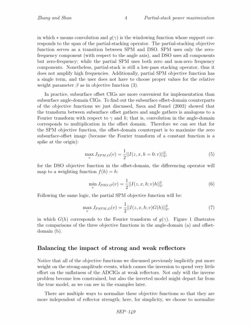
in which ∗ means convolution and g(γ) is the windowing function whose support cor-responds to the span of the partial-stacking operator. The partial-stacking objectivefunction serves as a transition between SPM and DSO. SPM uses only the zero-frequency component (with respect to the angle axis), and DSO uses all componentsbut zero-frequency; while the partial SPM uses both zero and non-zero frequencycomponents. Nonetheless, partial-stack is still a low-pass stacking operator, thus itdoes not amplify high frequencies. Additionally, partial SPM objective function hasa single term, and the user does not have to choose proper values for the relativeweight parameter β as in objective function (3).

In practice, subsurface offset CIGs are more convenient for implementation thansubsurface angle-domain CIGs. To find out the subsurface offset-domain counterpartsof the objective functions we just discussed, Sava and Fomel (2003) showed thatthe transform between subsurface offset gathers and angle gathers is analogous to aFourier transform with respect to γ and h; that is, convolution in the angle-domaincorresponds to multiplication in the offset domain. Therefore we can see that forthe SPM objective function, the offset-domain counterpart is to maximize the zerosubsurface-offset image (because the Fourier transform of a constant function is aspike at the origin):

maxv

JSPM O(v) =1

2||I(z, x, h = 0; v)||22; (5)

for the DSO objective function in the offset-domain, the differencing operator willmap to a weighting function f(h) = h:

minv

JDSO O(v) =1

2||I(z, x, h; v)h||22. (6)

Following the same logic, the partial SPM objective function will be:

maxv

JPSPM O(v) =1

2||I(z, x, h; v)G(h)||22, (7)

in which G(h) corresponds to the Fourier transform of g(γ). Figure 1 illustratesthe comparisons of the three objective functions in the angle-domain (a) and offset-domain (b).

Balancing the impact of strong and weak reflectors

Notice that all of the objective functions we discussed previously implicitly put moreweight on the strong-amplitude events, which causes the inversion to spend very littleeffort on the unflatness of the ADCIGs at weak reflectors. Not only will the inverseproblem become less constrained, but also the inverted model might depart far fromthe true model, as we can see in the examples later.

There are multiple ways to normalize these objective functions so that they aremore independent of reflector strength; here, for simplicity, we choose to normalize

SEP–149


Stack Power Maximization (SPM)

Partial SPM

DSO

Angle-domain, convolution

Offset-domain, multiplication

angle offset

(a) (b)

Figure 1: The comparison of the three objective functions in angle-domain(a) andoffset-domain(b). [NR]

SEP–149


them for each inline location x (Tang, 2011). The normalized version of objectivefunction (7) is:

maxv

JPSPM OB(v) =1

2

∑x

∑z,h [I(z, x, h; v)G(h)]2∑

z,h I2(z, x, h). (8)

The next step is to find the model gradient from the objective function, as we willuse gradient-based methods to solve this optimization problem. For conciseness andwithout bringing confusion, we omit the variables in I(z, x, h; v) and simply denoteit as I, and define

I =∑z,h

I2 and IG =∑z,h

I2G2(h). (9)

Then the gradient of the objective function (8) is

∂JPSPM OB

∂v=

∂I

∂v

(IG2(h) − IG)I

I2. (10)

Eq. (10) indicates that first we compute the image perturbation ∆I = (IG2(h)−IG)I

I2 ;then we back-project ∆I using the image-space wave-equation tomographic operator.

NUMERICAL EXAMPLES

We use the synthetic Marmousi model to test the effectiveness of the partial SPMobjective function. In our implementation, we use a two-way acoustic wave-equationpropagator, and for our optimization algorithm, we use non-linear conjugate-gradientwith Polak-Ribiere formula for search direction.

We implement the offset-domain representation of the partial SPM objective func-tion (eq. (7) and eq. (8)). The selection of weighting function G(h) is not unique, aslong as it can be considered as the frequency spectrum of a certain low-pass filter. Inour examples, we use Gaussian functions for G(h). We started with a wide G(h) thatwould include most unfocused energy of the ODCIGs at non-zero subsurface offsets,as the inversion proceeds, the gathers will become more focused; we then reduce thewidth of G(h) so that our objective function gradually approaches the traditionalSPM objective function. To control the resolution of the inversion, we preconditionthe model gradient with a triangular smoothing operator and reduce the extent ofsmoothing gradually within each iteration.

Marmousi Example

The model size is 9 km in x and 3.2 km in z. The spatial sampling is 20 m. The surveygeometry is of split-spread type, with sources and receivers located on the top of the

SEP–149


0 1000

2000 3000

0 1000

2000 3000

(a)

(b) Figure 2: The migrated image (a) using the velocity model inverted from the objectivefunction (7) (without normalization) and (b) using the initial model. The display clipwe use for (a) is 4 times of the clip used in (b), and we can see that in (a) the singlereflector marked in the left box becomes very strong and coherent. In contrast, manyweaker reflectors (for e.g., marked in the right box) that are initially present in theinitial image (a) are imaged much poorly in (b). Therefore it is important to give theweak reflectors more weight in the objective function. [NR]

SEP–149


model. There are 451 receivers with 20 m spacing that fully covers the model surface.We simulate 226 shots with shot spacing of 40 m. The central frequency of the Rickerwavelet we use is 10 Hz. For the inversion, we invert all frequencies simultaneouslyrather than from low to high frequencies. We run 40 nonlinear iterations for theinversion.

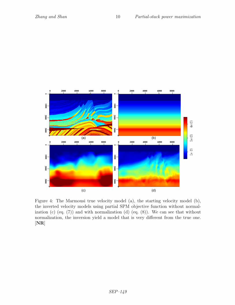
Figure 4(a) shows the true velocity model and 4(b) shows the starting modelv(z). Figures 4(c) and (d) show the inverted velocity model using the un-normalizedpartial SPM objective function and the normalized partial SPM objective functionrespectively. As we can see, the inverted result in 4(c) is stuck in local minima,because without normalization, the inversion will attempt to increase the focusnessof a few large, strong reflectors, while ignoring and even sacrificing the coherencyof smaller, weaker events. The observation of the corresponding migrated imagesin figure 2 further confirms our conclusion. The result in figure 4(d) shows globalconvergence towards the correct model. The long-wavelength part of the velocitymodel is well captured up to depth 2.2 km, as can be seen from the migrated imagesin figure 3.

CONCLUSION

We propose to use the partial stack power maximization objective function in wave-equation migration velocity analysis. This objective function merges the advantages ofboth conventional stack power maximization and differential-semblance-optimizationobjective functions, and it can achieve good global convergence, while retaining therelatively high resolution of the stack power maximization objective function. Wehave successfully applied our approach to the Marmousi model. We have also verifiedthat the normalization of the reflector amplitude in the objective function is not onlypreferred but necessary in the Marmousi case.

ACKNOWLEDGEMENT

The authors thank Chevron Energy Technology Company for the permission to pub-lish, and thank Yue Wang and Lin Zhang for suggestions and comments. The firstauthor thanks Prof. Claerbout for the initial discussion on WEMVA objective func-tions.

REFERENCES

Biondi, B. and P. Sava, 1999, Wave-equation migration velocity analysis: SEG Tech-nical Program Expanded Abstracts, 18, 1723–1726.

Biondi, B. and W. W. Symes, 2004, Angle-domain common-image gathers for mi-gration velocity analysis by wavefield-continuation imaging: Geophysics, 69, 1283–1298.

SEP–149


4000 0 2000 6000 8000

0 1000

2000 3000

4000 0 2000 6000 8000

0 1000

2000 3000

(a)

(b)

Figure 3: The comparison of the migrated images using the true velocity model (a)and using the inverted model with normalized partial SPM objective function (b).The two images match well up to 2.2 km depth. [NR]

SEP–149


0 1000

2000 3000

4000 0 2000 6000 8000

0 1000

2000 3000

4000 0 2000 6000 8000

0 1000

2000 3000

4000 0 2000 6000 8000 4000 0 2000 6000 8000

0 1000

2000 3000

(a) (b)

(c) (d)

Figure 4: The Marmousi true velocity model (a), the starting velocity model (b),the inverted velocity models using partial SPM objective function without normal-ization (c) (eq. (7)) and with normalization (d) (eq. (8)). We can see that withoutnormalization, the inversion yield a model that is very different from the true one.[NR]

SEP–149


Chavent, G. and C. A. Jacewitz, 1995, Determination of background velocities bymultiple migration fitting: Geophysics, 60, 476–490.

Clapp, R. G. and B. Biondi, 2000, Tau domain migration velocity analysis using anglecrp gathers and geologic constraints: SEG Technical Program Expanded Abstracts,19, 926–929.

Etgen, J., 1990, Residual prestack migration and interval velocity estimation: PhDthesis, Stanford University.

Fei, W. and P. Williamson, 2010, On the gradient artifacts in migration velocityanalysis based on differential semblance optimization: SEG Technical ProgramExpanded Abstracts, 29, 4071–4076.

Gardner, G. H. F., 1974, Elements of migration and velocity analysis: Geophysics,39, 811.

Sattlegger, J. W., 1975, Migration velocity determination: Part i. philosophy: Geo-physics, 40, 1–5.

Sava, P. and B. Biondi, 2004, Wave-equation migration velocity analysis. I. Theory:Geophysical Prospecting, 52, 593–606.

Sava, P. C. and S. Fomel, 2003, Angle-domain common-image gathers by wavefieldcontinuation methods: Geophysics, 68, 1065–1074.

Shen, P. and W. W. Symes, 2008, Automatic velocity analysis via shot profile migra-tion: Geophysics, 73, VE49–VE59.

Shen, P., W. W. Symes, S. Morton, A. Hess, and H. Calandra, 2005, Differentialsemblance velocity analysis via shot profile migration: SEG Technical ProgramExpanded Abstracts, 24, 2249–2252.

Soubaras, R. and B. Gratacos, 2007, Velocity model building by semblance maxi-mization of modulated-shot gathers: Geophysics, 72, U67–U73.

Symes, W., 2008, Migration velocity analysis and waveform inversion: GeophysicalProspecting, 56, 765–790.

Symes, W. W. and J. J. Carazzone, 1991, Velocity inversion by differential semblanceoptimization: Geophysics, 56, 654–663.

Tang, Y., 2011, Imaging and velocity analysis by target-oriented wavefield inversion:PhD thesis, Stanford University.

Tarantola, A., 1984, Inversion of seismic reflection data in the acoustic approximation:Geophysics, 49, 1259–1266.

van Trier, J., 1990, Tomographic determination of structural velocities from depthmigrated seismic data: 66.

SEP–149

wave-equation migration velocity analysis using partial

Documents