WAVE PROPAGATION IN LOSSY WAVEGUIDE STRUCTURES

bySteven E. Bucca

Thais submitted to the Faculty of theVirginia Polytechnic Institute and State University

in partial fulüllment of the requirements for the degree of

MASTER OF SCIENCE

in

Electrical Engineering

APPROVED:

"| .l

L' _«William A. Davis, Chairman

2

ISed i M. iad ary S. Brown

December, 1989

Blacksburg, Virginia

IIIII

WAVE PROPAGATION IN LOSSY WAVEGUIDE STRUCTURES

bySteven E. Bucca

Dr. William A. Davis, Chairman

Electrical Engineering

(ABSTRACT)

In this thesis a numerical technique is developed determining the propagation constant

in waveguides and transmission lines. The technique accounts for both dielectric and conductor

losses in a guide having an arbitrary cross section and uses a full-wave solution process. A set of

coupled, vector integral equations which characterize the system are derivecl. The equations

enforce the necessary boundary conditions on the tangential electric and magnetic fields at the

boundarics separating the conductors and dielectrics.

The method of moments (MOM) technique is used to cast the equations into a

numerically solvable form. Computed results for various waveguide structures are compared to

known or perturbed results for three well—known structures. However, the program is more

general and may be applied to other cross-sections. Finally, possible future extensions of the

work is presented.

E

Acknowledgements

iii

Table of Contents

INTRODUCTION ................................................................................................................. 1

PRELIMINARY TOPICS ...................................................................................................... 32.1 Introduction .............................................................................................................. 32.2 Vector Potential Representations of Two-Dimensional

Electromagnetic Fields in a Homogeneous and Isotropic Region ................................. 32.3 Helmholtz Integral Solutions for Two-Dimensional

Electromagnetic Fields .............................................................................................. 5

ANALYTICAL DEVELOPMENT ......................................................................................... 83.1 Integral Representations of the Electric Field via the ·

· Equivalence Principle 83.2 Equivalent Integral Representations

Integral Evaluation at Singular Points ..................................................................... 173.4 Integral Equation Solution to the Waveguide Problem ............................................. 233.5 Extension of the Waveguide Development to the Transmission

_ Line Problem .............................................................................................................. 26

NUMERICAL FORMULATION 314.1 Introduction ............................................................................................................. 314.2 Introduction to the Method of Moments ................................................................... 314.3 Moment Method Solution of the Waveguide Problem .............................................. 344.4 Summary ................................................................................................................. 45

iv

COMPUTER BASED RESULTS FOR THE WAVEGUIDE PROBLEM .............................. 465.1 Introduction ............................................................................................................. 465.2 Lossless Rectangular Waveguide ............................................................................... 465.3 Lossless Circular Waveguide ..................................................................................... 555.4 Lossless Ridged Waveguide ....................................................................................... 625.5 Lossy Rectangular Waveguide .................................................................................. 665.6 Summary ................................................................................................................. 71

SUMMARY AND CONCLUSIONS ....................................................................................... 73

REFERENCES .......;............................................................................................................. 75

DERIVATION OF VECTOR POTENTIAL REPRESENTATIONS ..................................... 76 ·

EVALUATION OF SINGULAR INTEGRALS ..................................................................... 79

NUMERICAL FORM DERIVATION ...................Q............................................................... 85

vmx ...............................................................................................;................................... 97

Q . V

I

I

Chapter 1

Introduction

Wave propagation in microwave guiding structures has long been a subject of interest.

Since the advent of the digital computer, the propagation effects due to cross-sectional

geometry and material properties have been widely studied. The computer has allowed the

study of waveguides having unusual cross-sections, multi-layered dielectrics, and multi-conductorI

paths. However, the effects of non-ideal conductors is an area that has not received such wide-

spread attention. _

‘ uThe most important effect of non-ideal conductors is signal loss. To quantify the loss,

I

umost researchers have used a perturbation approach [1,73]. With this approach the fields and

propagation constant are first determined for the lossless case and the loss is then approximated

by using the lossless fields at the conducting surfaces. Naturally, this teclmique is limited to

low—loss situations. In addition to creating loss, non-ideal conductors also modify the phase of

the signal. With the perturbation approach described above, this effect is completely ignored.

To fully account for the conductor effects, a more complete analysis is needed.

The analysis developed in this thesis determines the propagation constant in microwave

guiding structures. The resulting technique, a full·field analysis, allows the structure to have a

general cross-section and accounts for both conductor and dielectric loss. The full-field analysis

uses the vector potential representations of the fields and the equivalence principle [1,106] to

express the fields as integrals over the media boundaries in the structure (e.g. the

1

_ _

2

dielectric/conductor boundary). A set of coupled integral equations, which may be solved forthe structure’propagation constant, is obtained by matching the field components across theseboundaries. These integral equations are solved by using a popular numerical technique—themethod of moments (MOM). The MOM technique reduces the set of coupled integral equationsto a set of simultaneous linear equations, which may be solved by a number of well-known

techniques (e.g. LU decomposition —lower/upper triangularization).

Tl1e remainder of this thesis is divided into five chapters and three appendicies.

Chapter 2 develops the vector potential representations of electromagnetic fields. Chapter 3‘ clerives the coupled integral equations for both waveguides and coaxial transmission lines, with

special emphasis given to the waveguide problem. In chapter 4 the integral equations for the

waveguide problem equations are cast into a numerically solvable form, and chapter 5 presents

computer derived results for several waveguide structures. Chapter 6 snmmarizes the mainI- topics of the thesis and discusses theprimary conclusions. The three appendicies contain detailsA

of the derivations in chapters four and tive.

I Chapter 2

Preliminary Topics: Vector Potential gRepresentation of Electromagnetic Fields

2.1 IntroductionIn this chapter we ”lay the groundwork” for the upcoming analytical development.

The vector potential representations of electromagentic fields are presented, with a special

cmphasis on two·dimensional fields. In addition, terminology, definitions, and, coordinateI

’ systems are introduced.I

2.2 Vector Potential Representations ofTwo-Dimensional Electromagnetic Fields in aHomogeneous and Isotropic Region

Consider a homogeneous isotropic media characterized by a complex permittivity 6‘ and

complex permeability p'. Furthermore, let electric currents J and magnetic currents M exist in

the region. From the results of Appendix A, the electromagnetic fields ma.y be expressed in

terms of the magnetic vector potential A and electric vector potential F as i

E(r) = -vx1·*(r)+ ;%(v (V·A(r)) + k2A(r)) (2.1)

— .L. . -=’ 2.2H(r) - F(r)) +L F(r)) , ( )

3

V l

4

with

V2A(r) + /:2 A(r) = —J(r) (2.3)

V2F(r) + kz F(r) = —M(r) (2.4)

where r is the 3-dimensional position vector locating a point in space and kg E wz ;1'c'.

The del operator V may be conveniently defined as

- ^ QV - V„ + zöz (2.5)

where V,,. is the two-dimensional (transverse to operator. We now consider solutions to

equations (2.1) through (2.4) which exhibit wave propagation in the Z2 direction (two-

dimensional solutions). Specifically, we desire solutions where the z variation in all quantities is

given by c_]kZz ,_ -jk;Z —jkzZ 0E(r) = E(ß)¤ g H(r) = H(p)<= (--6a)

‘- kz - °k zy Jlr) = J(1>)¢ Z ' g _M(r) = M(1>)¤ Z Z (9-6b)

. ‘ _ - 'k z V - 'k Z .y A(r) = A(„)¢ J ‘_ , rn) = 1·‘(p)e J " (2.6c) _

where p represents the transverse to Zi component of the position vector r. The geometry

dependent parameter kg is an unknown quantity which must be determined. Only the values of

kg which satisfy Maxwell’s equations and the boundary conditions are valid; the purpose of this

thcsis is to find the allowed kg values for waveguide and transmission line problems.

The electric field E(p) may be expressed in terms of a Zi component and transverse

components as E(p) = E,,. + Eg2 (unless explicitly denoted otherwise, the implied argument

p will be dropped in the text that follows). If we substitute (2.6) into (2.1) through (2.5) and

A perform some elementary vector manipulations, we obtain

‘1

I ”5

and

Fu]? (Vu- (vtr ° Air) "'jkz Vtr Az + k2Atr) v (2*7b)

with

VÄA(P) + (*2 — l¤z°)A(1>) = —J(1>) (2-8) ·v.2ZF(1»> + (#2- (ss)

The equations for the magnetic field H(p) are similar to (2.7) and may be obtained via duality[1,98]. l

2.3 Helmholtz Integral Solutions for ·1 Two·D¤mensiona| Electromagnetic Fields ·

I° n ‘ Suppose we have two-dimesional sources acting in a homogeneous, isotropic, and

unbounded media (Fig. 2.1). The source coordinates are denoted by p' and the field coordinates

by p. The surface S denotes the area over which the sources act. For this case possible

. solutions to (2.8) and (2.9) are given by the two-dimesional Helmholtz integrals [1,228]

i 1 r (2) 1 1 :)A(ß) = jq J(1> ) H- (/¤1»I1>—1> I) ds (--10)S .

V1 1 (2) 1 1 .);_ F(1>) = jq M(1> ) H- (kpI1>·p I) ds - (--11)

SwhereHf,2)(·)

is the zeroth order Hankel function of the second kind

1c,, E lk2 - 1:,2(ls' is an element of area perpendicular to z.

I

6

YASource Point

EQ‘p' Pomf

. > X

Figure Coordinate system for 2—Dimensional field problems.

I

7

For the case where only surface currents exist on the boundary of the surface S (denoted by the

contour E — Fig. 2.1) then (2.10) and (2.11) become

1 I (2) 1 I 6) 6)A(1>) = Jg J(1> ) Hp (kp I1>—1> I) dk (--1-)E

1 1 (2) 1 I 6)F(1>) = j-; M(1> ) Hp (kp I1>—1> I) dk (--13)E

where dä' is an elemental length of the contour Z and § represents an integral over the

closed contour Z . _

II

Chapter 3

Analytical Development .

3.1 Integral Representations of the Electric Field via theEquuvalence Principle I

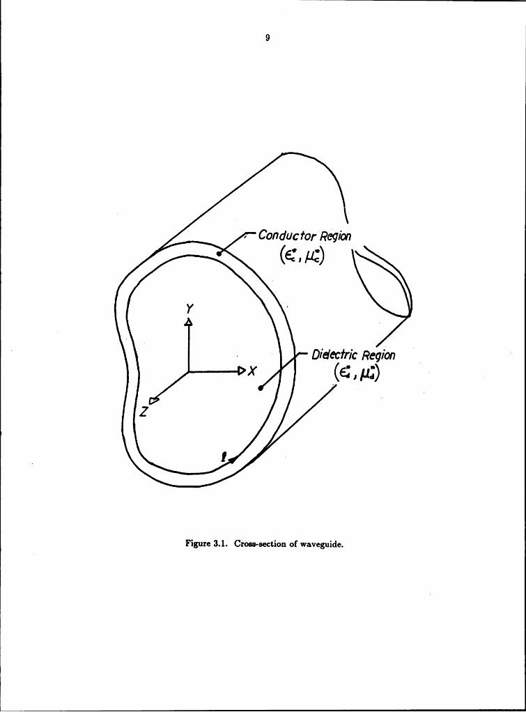
Consider the infinitely long (no variation with respect to z) source-free waveguide shown

in Fig. 3.1. Both the conductor and dielectric regions are assumed to be isotropic and

homogeneous. The dielectric, characterized by a complex permittivity ca and permeability pa,

supports the fields (Ed,Hd), while the conductor contains the fields (E°,II°) and is characterized ‘

by an equivalent permittivity 6}:1 and permeability pß. To simplify the- development we will V

· model the conductor as being infinitely thick. The model imposes no serious limitations provided

the actual conductor is at least several skin depths thick (this is case in most practical metallic

walled guides) [1,53] . _

To formulate the problem the equivalence principle [1,106] is used. We shall find thatI

the fields in the dielectric and/or the conductor regions may be expressed in terms of Helmholtz

integrals with equivalent sources on the interface between the two media. Tl1e required integral

equations are then obtained by matching the field components at the interface. In the

1Typically, conductors are characterized by a finite conductivity. The definition of 6;

implicitly includes the effects of the conductivity. For example, if the conductor has a

conductivity 0 and a permitivity co, then the equivalent permitivity would be

8 .

·

» Conducfor RéqionF (em;)®‘ i Didecfric Rcgibn 1

g 1

Figure 3.1. Cr0ss·secti¤n of waveguide.

° 310

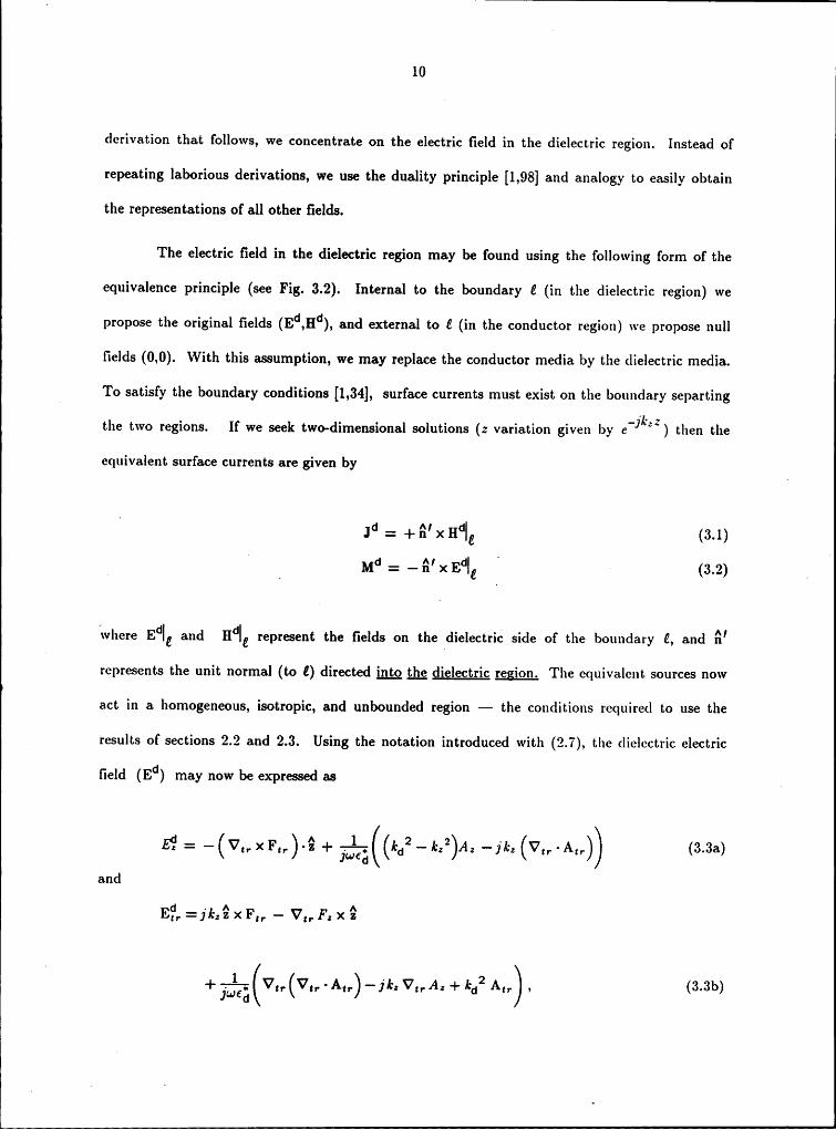
derivation that follows, we concentrate on the electric field in the dielectric region. Instead ofrepeating laborious derivations, we use the duality principle [1,98] and analogy to easily obtainthe representations of all other fields.

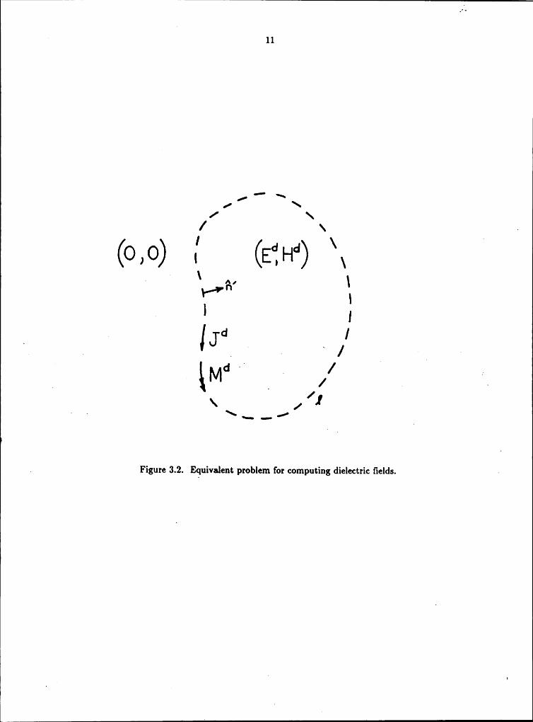
The electric field in the dielectric region may be found using the following form of theequivalence principle (see Fig. 3.2). Internal to the boundary Z (in the dielectric region) we

propose the original fields (Ed,Hd), and external to E (in the conductor region) we propose null

fields (0,0). With this assumption, we may replace the conductor media by the dielectric media.

To satisfy the boundary conditions [1,34], surface currents must exist on the boundary separting

the two regions. If we seek two-dimensional solutions (2 variation given by e_jk°z) then the

equivalent surface currents are given by

Jd = +6' X Hdl, (3.1)[ Md = -6'XEdI, ‘(3.2) [

{where Edl, and Hdl, represent the fields on the dielectric side of the boundary E, and ii,

represents the unit normal (to Z) directed into @ dielectric region. The equivalcnt sources now

act in a homogeneous, isotropic, and unbounded region —— the conditions required to use the

results of sections 2.2 and 2.3. Using the notation introduced with (2.7), the dielectric electricfield (Ed) may now be expressed as _

Ed = -(v,, X1·‘,,)-2 + A (1,,2 —k,2)A, —jk. (vg, -A,,.) (3.3a)]fA)€dand

Ed, :;/,.2 X r„ - v,,F. X Q

V,, (Vi, · A,.-)—1kz V,, Az + kdz A,, , (3-3b)]w€d

F11

1 / ·- \

// \

\ 6

' 6 6 \ 2<<>.<>> · <¤.H> .g I Jd ;

d = 6 / 2QM g ,/6 6 ‘ , / I

. Figure 3.2. Eguivalent problem for computing dielectric fields. .

312 3

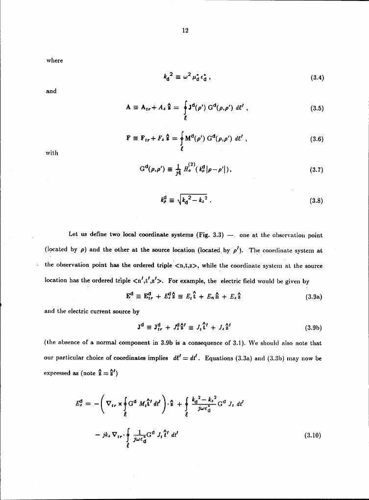
whereAdd E 6)** ,1;,2;,, (3.4)

and

A E A,,+ .4,2 = fJd(p') Gd(p,p') da' , (3.5)ä

F E F..+ F-2 = (M°(p’)G°(1>-ß') d(’ . (3-6). Z ·with

(F)H- (FS I1>—p’I)- (3-F)

16;,* E „|1.d2- 1.2 . (3.8)

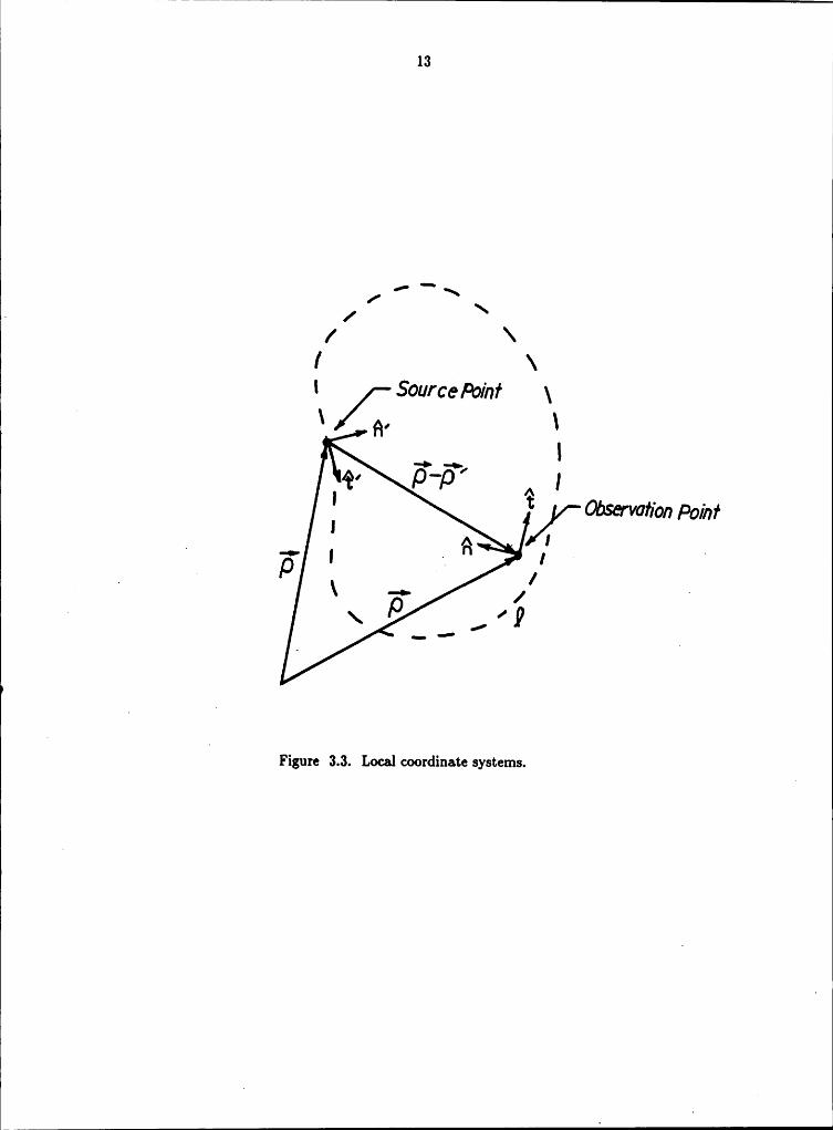
_ Let us define two local coordinate systems (Fig. 3.3) —. one at the observation point1

(located by p) and the other at the 'source location (located_ by p'). The coordinate system at ’

E - the obscrvation point has the ordered triple~<n,t,z>, while the coordinate systemlat

the source

location has the ordered triple <n',t',z'>. For example, the electric field would be given byEd E Ed, + E32 E 12,,2 + E,2 (6.96)

and the electric current source by1d E J?. + J32' E .1,’£' +

J.2’ (3.9b)(t-he absence of a normal component in 3.9b is a consequence of 3.1). We should also note that

our particular choice of coordinates implies dä,= dt'. Equations (3.3a) and (3.3h) may now be

€X[)l'6SS€d 6.S (IIOLC^1

1 A Id 2“ (W2 d rE3 M,1 az -2 J2 dtjwfdä ä

- jk.v,,-( +1-;cd 1,’£'az' (3.10)

e]L«J€d

13 I

A , ’ I \~/ \

I \\ /-Source Poinf \

—> —>‘

P‘P ’A 1

Observohon Porhf_ . I

. I p /·

1 [ P

U 1Figure 3.3. Local coordinate systems.

l14

and ‘

E7, E M, dt,

Z Z

+ V, V,az'rr Jwcä t tr jwfäZ Z

k 2+ fväcd 1,’£'dz' . (3.11)

We shall later see that our devlopment will require that the fields be eva.Iuated at the

boundary Z, posing a “slight” complication. When the observation point is brought to the

boundary, a point exists where the argument of the Green’s function Gd will vanish (see Eqs.‘ 3.5 -3.7). At this point the Green’s function contains a logarithmic singularity. For example, if

' — we lct |p—pf|·= P, then as P—>0 the Green’s function behaves as [1,203]h U ’

‘ (2)n

. k PG(k,,P)|p_,0 = j%H„ (k,,P)LD—>0 ¤ — gä. (C + ln%)] (3.12)

where C is EuIer’s constant (C=0.57721566...). At the singular point special care must betaken when manipulating the integral representations (equations 3.10 and 3.11). We address

this issue in the next two sections.

3.2 Equivalent Integral RepresentationsIn order to simplify the representations given by (3.10) and (3.11), we desire to

interchange the order of integration and differentiation in some terms. For this operation to be

valid, the Green’s function must exist and have continuous first order partial dcrivatives

[IL55?] . These conditions exist if the observation point is not gg the boundary Z. To allow

1 n15 I

the interchange, the observation point is assumed to lie in the dielectric region a small distance

6 away from Z. In Section 3.3 we investigate the case where the observation point approachs

the surface (6—> 0).

Consider the first term of (3.10), l

— (v„X ]G°(d.p') M.(p')€'dv)·d = —]1 dv. (3.13)Z Z

Since V1,. does not operate on the primed coordinates, the term reduces to

(V„Gd)></Ii, . The right hand side of (3.13) now becomes

AX v)M.(d') d1' . (3.11)g 1

— — Since Gd(p,p') is a function of ]p—p'] (see 3.7), V,,Gd(p,p') iseqniyalent to . I .

v.. G°(p.1>')= —v£. ¤°(p.d') (3.13)

where V],. operates on the primed (source) coordinates [6,497]. Using our local coordinate

system (Fig. 3.3),

_ 1 11 1 ^1.^..- @*1 <i<£‘^1^1.^--@.@i‘ 316((V,,.G(p,p))xt)z- ]:(ön,n+öt,t)xtj]z- önl. )

Equation (3.13) now becomes

d I— ( V1. >< [61661) M.(p’)?’ dv ) · 2 = ] ‘2%-fl M„(p’) dv. (3.11)Z Z

16

For an expression similar to the third term in (3.10) we have

Av dv = —f [(v:.¤"<p.1»'> )-€')] d.<1v> dv . 13.181Z Z

But,

d 01vged , ·.2·]1

· :1 @@-:2 1 od -¤¤4[( t (pp)) t(p) tät; öt;( t ) ät;

so (3.18) becomes

1,(„')’£'

av d1'+ dv. (3.19)Z Z Z

since the current and the Green’s functions are single valued functions, the first term on the

. right hand side of (3.19) evaluatw to zero. Thus, (3.19) becomes ° i

I?' dt' dv . <ß.20>Z Z

Using (3.17) and (3.20) we may write equation (3.10) as

d k 2_ k 2E?ön JW€d .Z Z

.u

6J- 1,} 4äG° 4 dt' . 3.21Z

From matching the tangential field components at the interface, we note only the 2

and it components of the fields are required in our development. By taking the dot product of

I

17

(3.11) with li and using the concepts of this section, the following equation is easily derived:

_ dEf = -)k, {Gd M, dt'Z Z

Q 1 d Q 1_ - Q 1 u 1+ Ö, dt gk, 8, jweäf} J, dtZ Z

162+§%o"1,(’£'-’£)41' . (3.22)]W€d

Z

3.3 Integral Evaluation at Singular PointsThe forms of (3.21) and (3.22) are still not the surface fields needed for the boundary

conditions. The observation point must be brought to the surface, where the integrals contain a

singularity, making numerical · evaluation difficult (if not impossible). A To solve this

complication, we separate each integral into the sum of two integrals. If we let 26 be a small _ -I

section of Z centered on the singularity, then our integrals may be written as

1 1 +€1(·)dt; I(·)dt+ (·)dt, (3.23)-6

V Z Z—26

where ( · ) denotes the integrand of interest. The topic of this section is the evaluation of the

second integral on the right hand side of (3.23). The remaining integral of (3.23) does notcontain a singular point in its interval of integration and may be evaluated using numerical

techniques.

To evaluate the singular integral, the following technique is used. As shown in Fig. 3.4,

the observation point is located within the dielectric region, centered in the small interval 26,

and displaced a small distance 6 away from the boundary Z . If 6 and 6 are sufficiently

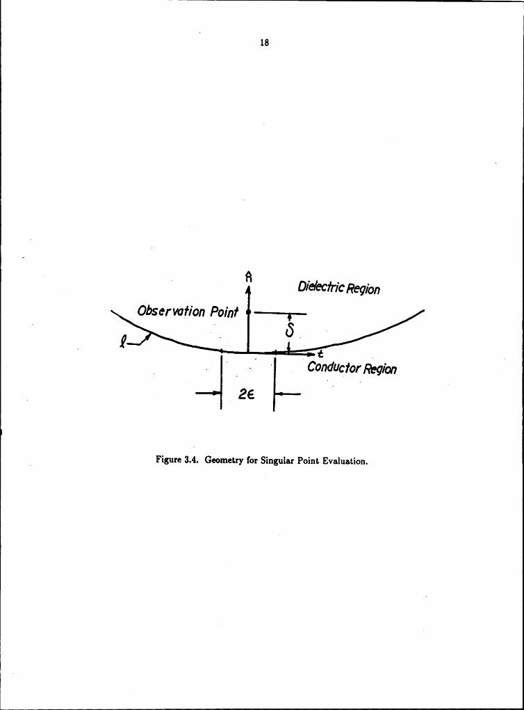
G18

i A . , _4 Ü/ÜGCÜICRegion vObservation Point —;——

a 4 .a ’4 e r O Condveior Region

_ 26 i O

4 Figure Geometry for Singular Point Evaluation.

. F

19

small, then the singular integrals may be approximated by using small argument expansions of

the GP€CH,S function and currents. Once the integrals are evaluated, the fields are forced to the

surface by imposing the condition 6 —•0 . Finally, the integral contribution is made exact by

letting the patch size 26 approach zero, providing a resultant Cauchy principle value form of

integration.

The integrals of interest are (see equations 3.7, 3.21, and3.22)_

_ +6 (2) dv (3-24)

+6 (2)ÄPO ÖIÄFPO Ho (kgl/*‘P'F) dt, (3-25)

‘ r _+6 (2)

i_ * °1 1* 1* 1 ' L-Ö-11 kd - ' dt' 3.26pl)_

_ +6 (2) dv (3-21)

where I(p') is either a surface current or a surface derivative of the current. In Appenclix B the

above integrals are evaluated, allowing equations (3.21) and (3.22) to be written as ,

Ed Mr öGd 1 kd2"k-=2 d 1-· än Jwfd

Q Q

(- jk, (Ac-d id!) dv (3-38)

e]‘·<·’€d

ät

u

20

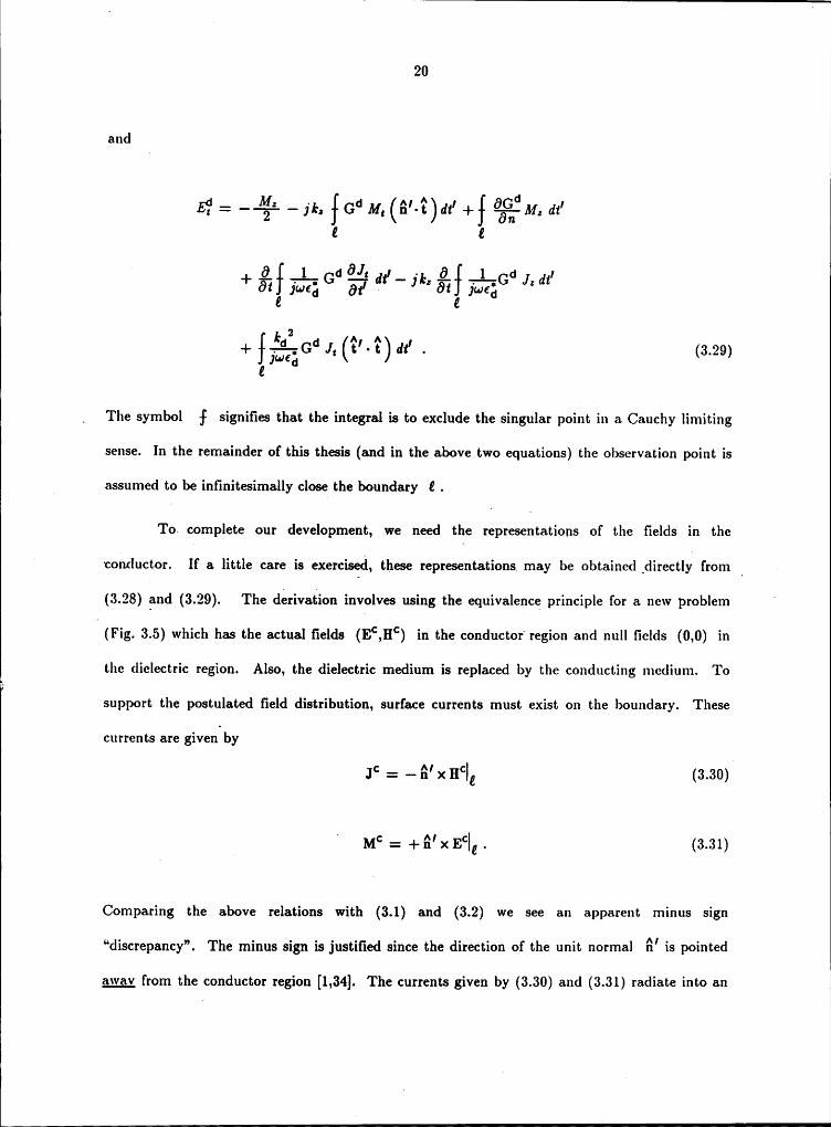
and

dE? = --2% - jk, {od M, (ä'-’£).1z' +{ az'Z Z

dt gk, ät jw€äG J, dtZ Z

k 2+ ][$1Gd J, (I' ~ dt' . (3.29)ywcd

Z

_ The symbol { signifies that the integral is to exclude the singular point in a Cauchy limiting

sense. In the remainder of this thesis (and in the above two equations) the observation point is

assumed to be infinitesimally close the boundary Z . .

To. complete our development, we need the representations of the fields in the

conductor. If a little care is exercised, these representations. may be obtained directly] from } e

(3.28) and (3.29). The derivation involves using the equivalence principle for a new problem 'I(Fig. 3.5) which has the actual fields (E°,H°) in the conductor region and null fields (0,0) in

the dielectric region. Also, the dielectric medium is replaced by the conducting medium. To

support the postulated field distribution, surface currents must exist on the boundary. These

currents are giveni by

J° = -ä' xH°I, (3.30)

° M° = +8'x1:°|, . (3.31)

Comparing the above relations with (3.1) and (3.2) we see an apparent minus sign

“discrepancy”. The minus sign is justitied since the direction of the unit normal fi' is pointed» awav from the conductor region [1,34]. The currents given by (3.30) and (3.31) radiate into an

21

a f °\é \’

\/ \ —

(E +4 ’ ‘I i } \

\ 1 \H1

l 1

’ 1 °‘ 1 / . ‘

„ \i

Figure 3.5. Equivalent problem for computing the conductor fields.l

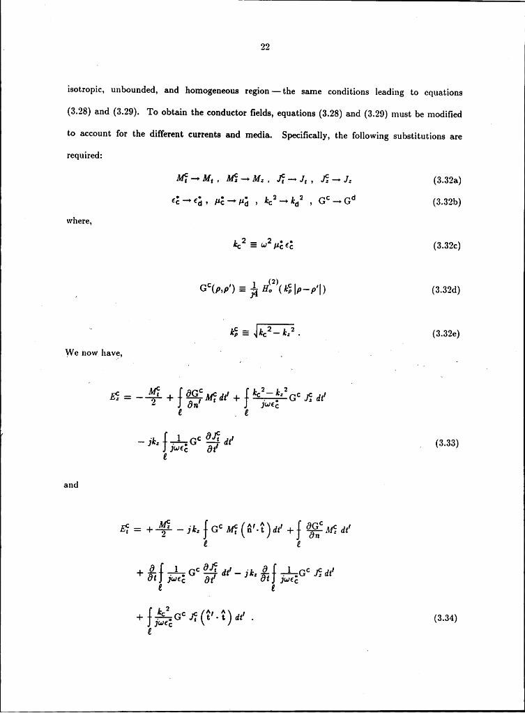
_ 22

isotropic, unbounded, and homogeneous region—the same conditions leading to equations(3.28) and (3.29). To obtain the conductor fields, equations (3.28) and (3.29) must be modifiedto account for the different currents and media. Specifically, the following substitutions arerequired:

M$—»M,,ME—M,,1$—1,,1$—»1, (3.32a)::3-.:;, ,1;-:,1; , 1:3-.1:,,* , c;‘=-»c;° (3.32b)

‘ where,

1:3 E :3 ,1;:; (3.32c)

c 1 - 1 (2) c 1 qG (mp) = jq H: (/¢:»I1>—1>I)We

now have, ' . i -I

_

” 2_ 2 IEE: —&+;I@:Mfdt'+][&Ä-G°JEdt'2 Ön Jwfc »

Z , Z

. [- 1: ][4„G° —ldt _ 3.33Z

and ‘ ”

Ef = 1.-%% —jk,][G° 1:1s(6·.@).1:· 1.} *%*11; dt'Z Z

Q 1 c I_ · Q l c I+ Öi][ jwcä G 3{ di jk; Öi][ju.16§GZZ

k 2 c ^I ^ I+][—:%G .]$(t ·t)dt . (3.34)Z Jwfc

[l

23

We note that the terms (see 3.28 and 3.29)

% and -1% (3.35)and the corresponding terms in (3.33) and (3.34) appear to have conflicting signs. Recall, theabove terms resulted from the integrals (3.25) and (3.26). In the calculation of (3.25) and

(3.26), the derivatives were calculated with the observation point approaching E from within

dielectric region. However, the conductor fields must be forced to approach the boundary

from within @ conductor region. In this case the normal derivatives are taken on the opposite

side of E, creating the negative signs in question. The proof is straightforward with the

observation point located at n= — 6 (see Fig. 3.4) and following the approach given in

Appendix B. ‘

3.4 Integral Equation Solution to the Waveguide ~ 2Problem . _ _ 2 „

( l ' Unless the conductors are perfect, the li and 2 componentsof the fields arc continuous I

across the boundary [1,34]. This condition requires l

V EQ : E; and E? = E? (3.366,)

and

Hg : H§ and H? = H? . (3.36b)

Using (_3.36) with (3.28), (3.29), (3.33), and (3.34) gives,, d le 2- le,2 ,1, ae'

·· ön -7""dE Z

. Ü] Mc ÖGC 1— le, -4 dt' = --4 ][—-Mcdtf llwéd 0z’ 2 + 6m' ‘E E2 2älicf JS de'- jk, [A16? Ü? de' (6.67)

Z Jwfc £J¢•l€c Öl

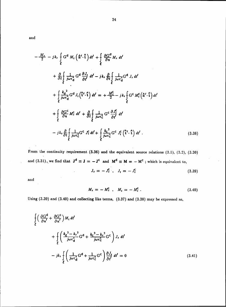
24

and

ujk; {Gd M, dt,2 Z

1 Ö Ö']!l,

_ • 1 d I+ ät; jw€äG E? dt gk, ät! JTQG J,dt

2 2 ‘1, (’£'-2)12'2° 2

1 Q 1 c Ü}? 1Z

_ ~. Q 1 c 1 kcz c ^1_^ 1gi. öi][T-wege Jgdt + LTEG 1;* (2 2) dt . (3.38)Z Z

I2‘rom the continuity requirement (3.36) and the equivalenit source relations (3.1), (3.2), (3.30)_ and (3.31),_we find that Jd E J = —Jc and Md E M = — Mc ; which is equivalcnt to,

l °2 . J, = —J‘§·~, J, = —J$ (3.39)

and Q »M,=-—M§, M,=—M$. (3.40)

Using (3.39) and (3.40) and collecting like terms, (3.37) and (3.38) may be expressecl as,

@2 & M Mlt(ön' + 811, ) i

Zgc 2_ kl? 2_ 2

+ ][ (—Gd+ E;°i-GC) J, dt'](«ü€d ]üJ€cZ

2 —— jk,} T%G"+-„l-,c;° Ü; 12' = 0 (3.41)a

]w€d Jwfc Ü!

l

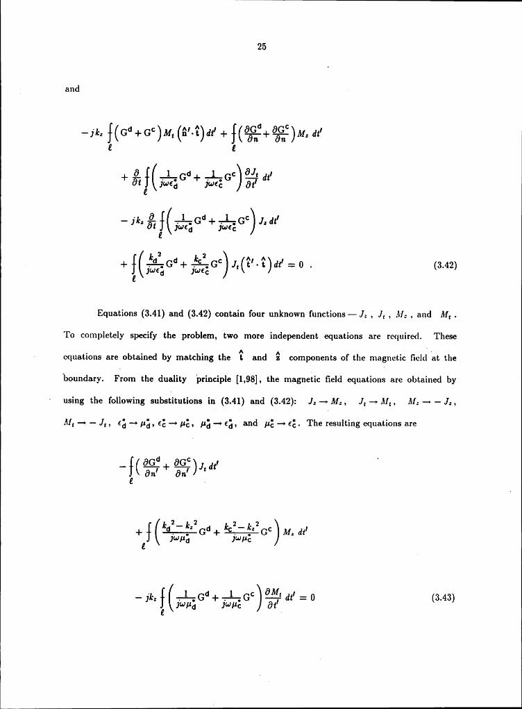
25

V and

_ - d c ^1_^ 1 6Gd öG° 1Z Z

-.1,Gd+ -.1,Gcdt,

6t Jwcd ywcc ät'Z

J; di,]W€d ]ü)€c

Z

k 2 2+)[ -Gd+¥G° J,(’t'·’t)dt'=0 . (3.42)Z

]w€d ]Lü€c

Equations (3.41) and (3.42) contain four unknown functions- J; , J, , M, , and M, .

To completely specify the problem, two more independent equations are required. These* equations are obtained by matching the lt and Q components of the magnetic fiel6l

fatthe,

boundary. From the duality principle [1,98], the magnetic field equations are obtained by

* using the following substitutions in (3.41) and (3.42): J,-Mz, J,-M,, MZ- —J,,

M, —> —— .],, 6; —-> 11;, cf; —-> 11;, 11; —> 6;, and pf; —» cf; . The resulting equations are

66;** 6G° 1 °— - + -- J dt][(671, 611l ) t

g .

M., dt,Jwßq JW/JcZ

— jk,] -1-Gd + -G° 2% dt,= 0 (3.43)

Z Jwßd Jwllc 6t V

26

and· ¤ <= ^I.^ I - QCE ÖE I+;kZ ((6 +6 an + an )1.«1I

Z Z Z

. äM%dt’Z 2l Jwßd Jwßc 6:

eJwßd Jwlßc

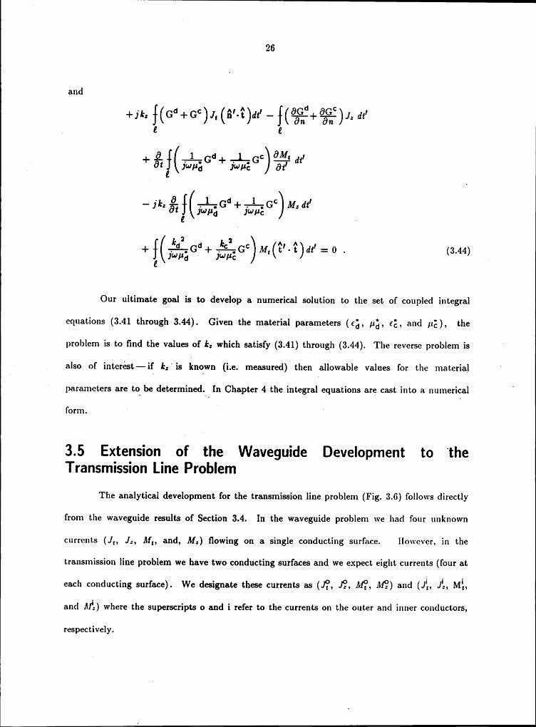
1+ 2 ( I+1: +g1Gd+Ä·G° M,(I'·/tl)dt'=0 . (3.44)E

Jwßd Jwßc

Our ultimate goal is to develop a numerical solution to the set of coupled integral

equations (3.41 through 3.44). Given the material parameters (6;, pg, cß, and pß), the

problem is to find the values of IcZ which- satisfy (3.41) through (3.44). The reverse problem is ‘

_ also of interest~—if kZ'is known (i.e. measured) then allowable values for the material ‘

parameters are to be determined. In Chapter 4 the integral equations are cast into anumericalform.I °2 3.5 Extension of the Waveguide Development to the

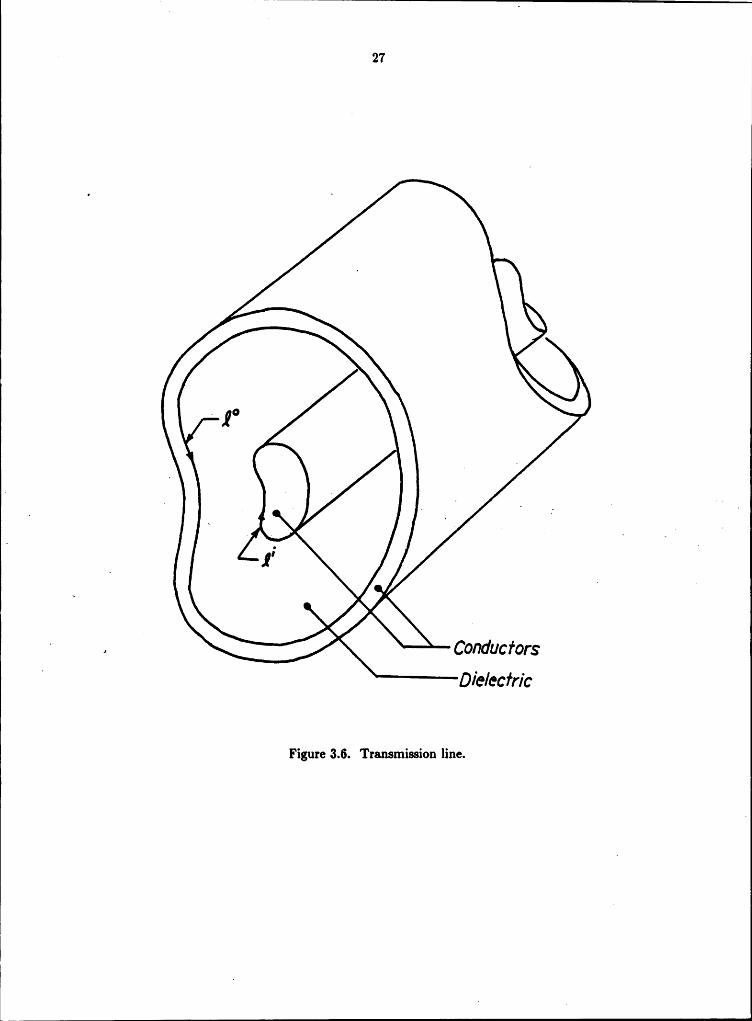
Transmission Line ProblemThe analytical development for the transmission line problem (Fig. 3.6) follows directly

from the waveguide results of Section 3.4. In the waveguide problem we had four unknown

currents (J,, JZ, M,, and, MZ) flowing on a single conducting surface. Ilowever, in the

transmission line problem we have two conducting surfaces and we expect eight currents (four at

each conducting surface). We designate these currents as (Jg, Jg, Mg, Mg) and (J), JlZ, Mi,

and MlZ) where the superscripts 0 and i refer to the currents on the outer and inner conductors,

respectively.

L27

i C.Die/ccfric

Figure 3.6. Transmission line.

· I

° 28

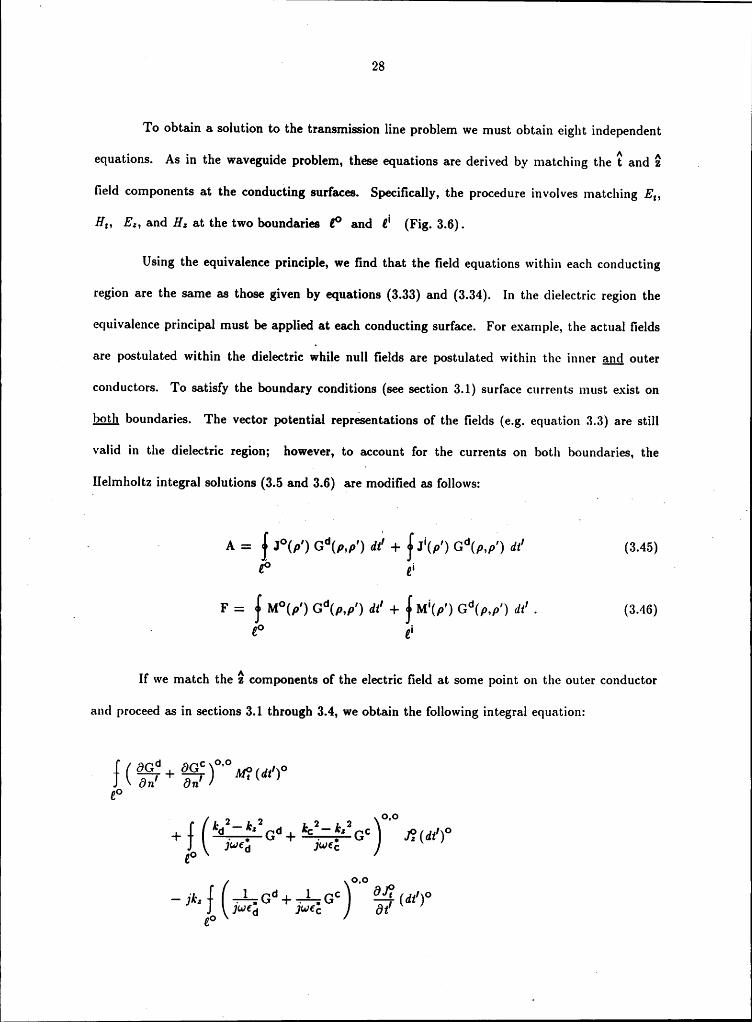
To obtain a solution to the transmission line problem we must obtain eight independent

equations. As in the waveguide problem, these equations are derived by matching the ll and iz .field components at the conducting surfaces. Specifically, the procedure involves matching E,,

‘ H,, EZ, and HZ at the two boundaries £° and Zi (Fig. 3.6).

Using the equivalence principle, we find that the field equations within each conducting

region are the same as those given by equations (3.33) and (3.34). In the dielectric region the

equivalence principal must be applied at each conducting surface. For example, the actual fields

are postulated within the dielectric while null fields are postulated within the inner arg outer

conductors. To satisfy the boundary conditions (see section 3.1) surface currents must exist on

both boundaries. The vector potential representations of the fields (e.g. equation 3.3) are still

valid in the dielectric region; however, to account for the currents on both boundaries, the

Helmholtz integral solutions (3.5 and 3.6) are modified as follows: _

( — · A = i J°(ß') G°(ß•ß') dt' + i J‘(1>') G°(ß•p') dt' (345) A

_ F dt' - (346)

If we match the 9 components of the electric field at some point on the outer conductor

and proceed as in sections 3.1 through 3.4, we obtain the following integral equation:

@2 „. @.*3 °·° Mo ,„· <>I l[(än' än') i()ÜO

2 2-2.3 .„ 2 ,.+][ J-G +—Gc .]?(dt)]¢J€d ]Ul€ceOo,o Jo

- jk.} %c;**+%c;° E (dt')°o

J¢··'€d J‘·¢€cät

E

A1

29

Gd oiif(dt')'_ 811, i _ 7***6:;

Z1* 2*· o,i aj— jk, § (LG') (dt’)' = 0 (3.47).7***6 Üi1* d

where the single superscript, o or i, represents the appropriate quantity at the outer or inner

surface, respectively. The double superscripts designate the surface at which the observation

point is located and tl1e surface over which the source exists. For example, the double

superscript (o,i) implies the observation point is located at some point on the outer surface @°

and the source exists on the inner surface Z'. If we match the[ti

components of the electric field

at some point on theouter surface, we obtain ·0,0 .-11,]* (6***+6**) M$_(6*-’£)°·°(61')° 1

@9 — ‘, . ‘ ” i .ind c ¤„¤ G n .

I 1 J-. + ,1 (äßg) M2 (.6*)<>

E° ‘ i0,0 l

.6*. ...1 ¤ ....1 ¤ Q?·¤+öti(jw€äG + jU€éG ät' (dt) -_ E0,0_ · . Q 1 6 1 c 1 o

E0,0k 2 ],· 2 A A I

e° d I C

,' . - . d o,i . .-161(Gd)°'1G<*·'·*>°·'<*=’>'+ 1%) *1** <**’>'1:* e*

°" 61*ö § 1 6 « 1 a+ ·—· 1- dtöt

I

30

o,i_ — Q 1 d ‘ 1 1,1-. Ö,EIk 2o,i4-(Täod 1; (S'- «)°·' (dt')' = 0 . (3.48)

-]w€d

. g'

By simply switching the superscripts (0-+i and i—+o) in equations (3.47) and (3.48) we can

obtain two more independent equations. The resulting equations are equivalent to those

derived by matching the lt and Q components of the electric field at the inner conductor. The

final four equations are found by matching the/S and 2 components of the magnetic field at the

two surfaces. Once again, these equations may be easily obtained by applying the duality

principle to the electric field equations.

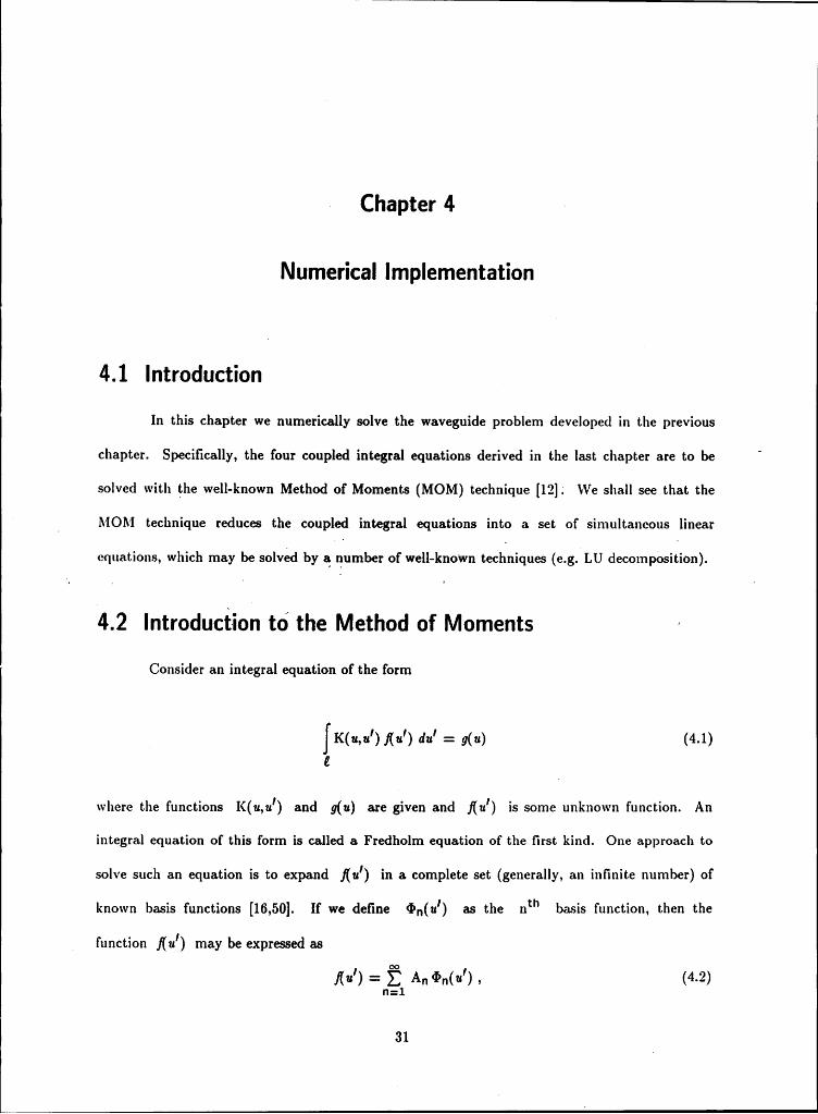
Chapter 4 1

Numerical Implementation

4.1 IntroductionInthis chapter we numerically solve the waveguide problem developed in the previous

chapter. Specifically, the four coupled integral equations derived in the last chapter are to be '

solved with the well-known Method of Moments (MOM) technique [12]; We sha.ll see that the

MOM teclmique reduces the coupled integral equations into a set of simultaneous linear

equations, which may be solved by a number of well-known techniques (e.g. LU decomposition).

4.2 Introduction to the Method of Moments (Consider an integral equation of the form

]1<(„,„') j(u') 41/ = g(„) (4.1)E

where the functions K(u,u') and g(u) are given and j(u') is some unknown function. An· integral equation of this form is called a Fredholm equation of the first kind. One approach to

solve such an equation is to expand f(u') in a complete set (generally, an infinite number) of

known basis functions [16,50]. If we define <I>„(u') as the nm basis function, then the

V function f(u') may be expressed asKu,)

= An ¢n(u’),t1=1

31 _

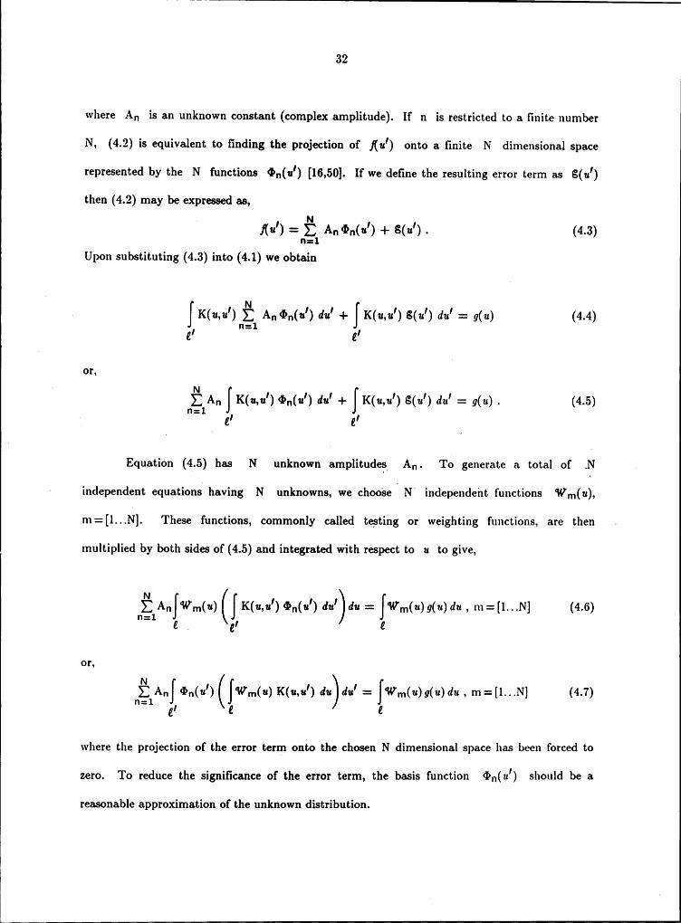
I32

where An is an unknown constant (complex amplitude). If n is restricted to a finite number

N, (4.2) is equivalent to finding the projection of j(u') onto a finite N dimensional space

represented by the N functions <I>„(u') [16,50]. If we define the resulting error term as S(u')

then (4.2) may be expressed as,I N I Ij(u) =n;1 An <I>„(u) + 8(II ) . (4.3)

Upon substituting (4.3) into (4.-1) we obtain

I N I I I I IK(u,u) E An <I>„(u) du + K(u,u ) 8(II) du : g(u) (4.4)fl:].el ‘ Z]

or,N I I I I I IE An ([K(u,u ) <I>„(u ) du + ]‘K(u,u ) 8(I1 ) du : g(u) . (4.5)

I‘l=1 I' I'

_ Equation (4.5) has N unknown amplitudes An. To generate a total of -N

- independent equations having N unknowns, we choose, N" independent functions ‘Wm(u),

m=[1...N]. These functions, commonly called testing or weighting functions, are then .

multiplied by both sides of (4.5) and integrated with respect to u to give,

Ndu') du g(u) du , m= [1...N] (4.6)"zl I I

or,N2:1.4,,], <I>„(u')-( K(u,u') du) du, = [‘Wm(u) g(u) du , m: [1...N] (4.7)"‘ er I I

where the projection of the error term onto the chosen N dimensional space has been forced to

zero. To reduce the significance of the error term, the basis function <I>„(I/) should be a

reasonable approximation of the unknown distribution.

[ Z l

· _ 33

Equation (4.7) may be compactly written as

N‘ nglzmn An = vm, XH=[1...N]

,where_Zmn E {[<I>„(u') ([‘Wm(u) K(u,u') du) du, , (4.9)

e' ¢

and '

A Vm E [‘Wm(u) g(u) du . (4.10)Z

In matrix notation we have[Z] ·[A] = [V] (M1)

[„_ ” where [Z], [A],

land[V] are NXN, Nxl, ‘ and Nx1’ matrices respectively. Once the ·

I ° .

elements of — [Z] and [V] _ are obtained,—the unknown coefficients [A] may be determined

by using an algorithm such as LU decomposition.

The choice of expansion and testing (weighting) functions is an important topic. In the

above discussion it was noted that the expansion function should reasonably approximate the

unknown function. The testing function should be chosen such that small variations in the

testing location (the testing function’s interval of integration) does not cause significant changes

in [A]. The particular choices should also represent a balance between accuracy and efficiency

[10,187]. In general, clear·cut rules on this topic do not exist. Some widely used expansion

functions include the pulse and triangular functions (see the next section and [10,188]), while

comonly used testing functions include the pulse and Dirac delta functions.

34A

4.3 Moment Method Solution of the WaveguideProblem

I The first step in numerically solving the problem of interest is to approximate the

boundary ll by a discrete set of Nipoints: #11 n = [1 ,...,N] (Fig. 4.1). By connecting adjacent

points with a straight line we form N linear segments. The segments are referenced as Aßn,

n = [1 ,...,N] where the nth segment is defined by the points #, and #,+1 . These segments,

having the lengths An, n = [1,...,N] , are characterized by a set of local coordinate systems° having constant tangential and normal vectors.

Next, we approximate the currents by defining basis functions along each segment.

From equations (3.41) through (3.44) we find that the current functions we must approximatehave the forms . _

. 1 I;(t'), I,(t'), and , . ‘ (4.12) 1 ‘

where [,(t') and I1(t') represent either an electric or magnetic current. For simplicity we

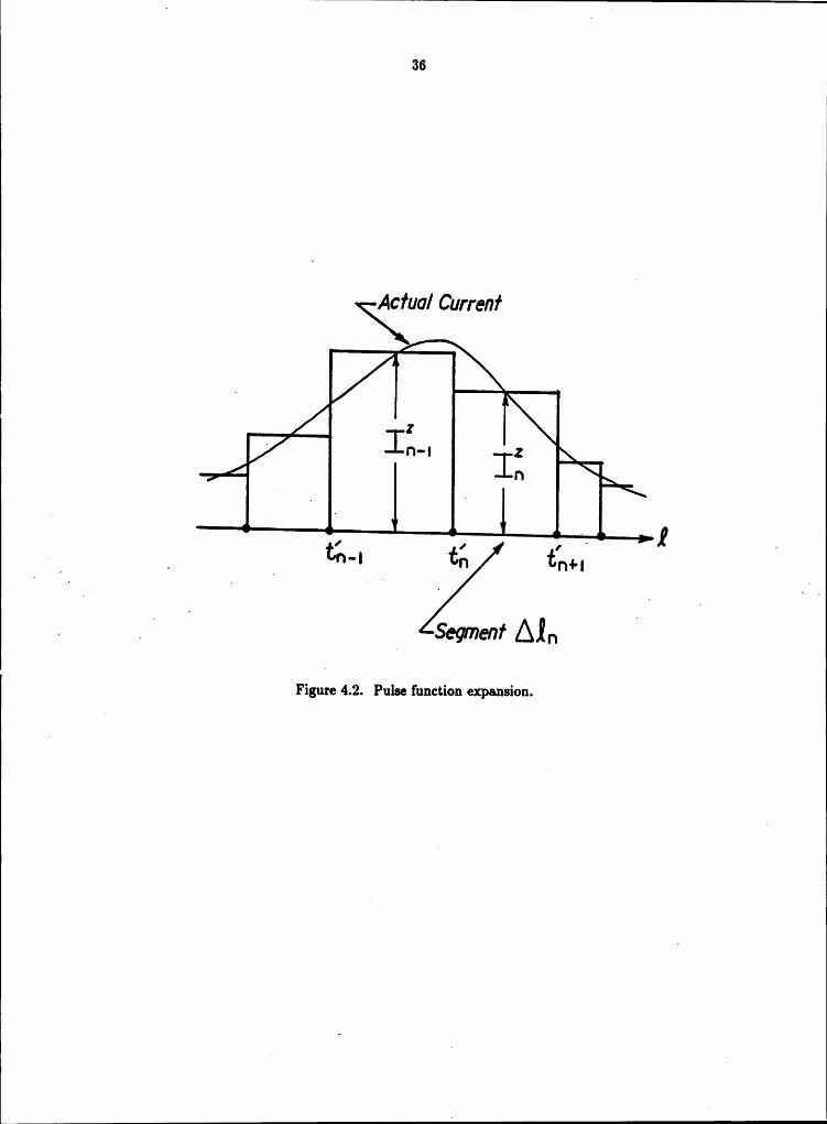
shall. expand the currents represented by I,,(t') by a summation of pulse functions.

Specifically, we haveI

N 1 for z' in Aa uI,(t') = E I1§P,,(i') , P„(t') = {

n (4.13)"=1 0 elsewhere

where the Iä 's are complex amplitude coefficients. The pulse expansion of (4.13) is equivalent

to a “stair-step" approximation of I,(t') as shown in Fig. 4.2. Since we must approximate

I1(t’) and its derivative, the pulse function expansion is not appropriate for this current. We

need an expansion function that gives a continuous approximation to the current. A relatively

lA 35 '

Seqmenf AII„Iin

. {-INI I - ~ ~‘·I

\ {ml\1/ \\

Ol\

II

g \ II .I .

{ I · .. , ‘

A I" 5 , *-2 „

. I. / -

· x >‘Y '

II 1, A1llt~~.

Figure 4.1. Discretizatiou of boundary.

36

Acfuol Currenf

A Z

g ,1

1 Z A1 Segmenf

Figuie 4.2. Pulse function expansion.

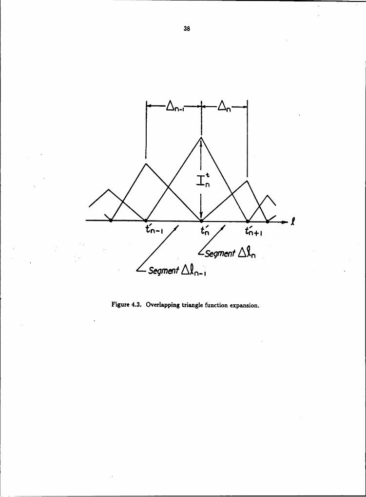
137

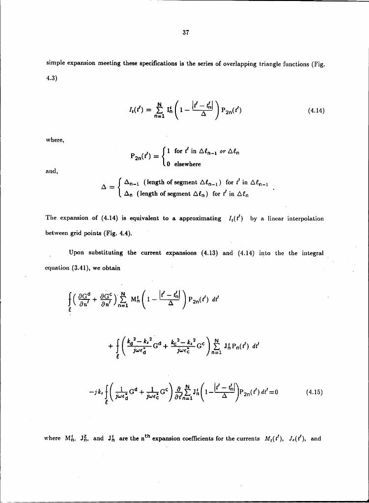
simple expansion meeting these specifications is the series of overlapping triangle functions (Fig.4.3)

N z' — z'I,(t') = n;1 I}, (1-ä P2n(t') (4.14)

where, u

1 for t' in A2 _ or AEP2„(¢’) ={ " ‘ "0 elsewhereand,

A _ A,,_, (length of segment AZ„_,) for tl in A£,,_,An (length of segment AZ,,) for t' in Aün

i

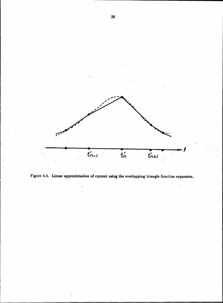
The expansion of (4.14) is equivalent to a approximating I,(t') by a linear interpolation

between grid points (Fig. 4.4).

_ Upon substituting the current expansions (4.13) and (4.14) into the the integral IU

ecluation (3.41), we obtain ‘ ‘ -I _!

ÖGd ÜGC ‘ N 1lt, ' liwl 1 1 »—— + —— M 1- ———— P l dtn A 2n( )

+][ ·g—=·7—G +—r¥Gc J‘P t, dt,nä

nN

l1’ — 1’|1* 1---2 P tl dt':0 4.15.7 Z ötyngl I1 A 2n( 7 ( )

where M}, Jä, and J}, are the nth expansion coefficients for the currents M,(t’), J,(t’), and

i 38I

,"An—•"°|"An‘] I‘

A4 ,e Seqmenf AQ,-,-3, F ·

Figure 4.3. Overlapping triangle function expansion.

39

I I ·—

\I \1, ‘[.

/I

VI

/

.>

- „II I } ’ ‘

I Ü 3 _ — tn-! g tn tm-I _

Figure 4.4. Linear approximation of current using the overlapping triangle function expansion.

I40

J,(I'), respectively. In the discussion that follows, the observation point will be designated as I(recall that this point is on the surface Z). As explained in section 4.2, we use N independent

weighting (testing) functions to generate N independent equations. For simplicity, we let the

weighting function for (4.15) be given by

, m=[1...N]. (4.16)

I In words, (4.16) states that the weighting function for (4.15) is a delta function that is locatedat the midpoint of the segment defined by the grid points IQ and 1%+1 . Next, the product

of (4.16) and (4.15) is integrated with respect to I. If the segment of integration is the chosen

to be AEm_ we obtain

· tl{|'I+1 _ - I Am · _(equatnon 4.15) 6(I— Im-?) dt, m = [1...N] . (4.11)4 z„,' _ _ “ _ .

In Appendix C we show that (4.17) is equivalent to

NE M:. (02... + ¤$„„)I1:].

~ 4*-1:.* d 1*-1*+ J ‘ L-TB + ie-—-;L B°ngl n mn Jwfc mn

N-1 1* %c° +4%c° :0, :1...N 4.187 zn;1 n(]w€d mn Jwfc mn m I I ( )

where the “constants” Agg), Bää),Cgfä), are defined in the appendix. By inspection, the

141

numerical form of the dual equation (3.43) isN-2: J:. (4:*.... + A:..„.)I1:].

~ Ic 2- 11.2 1. 2- 1. 2+ M' &?B" + BCngl n ( Jwpd mn Jwpc mn

n=1 Jwßd Jwßc

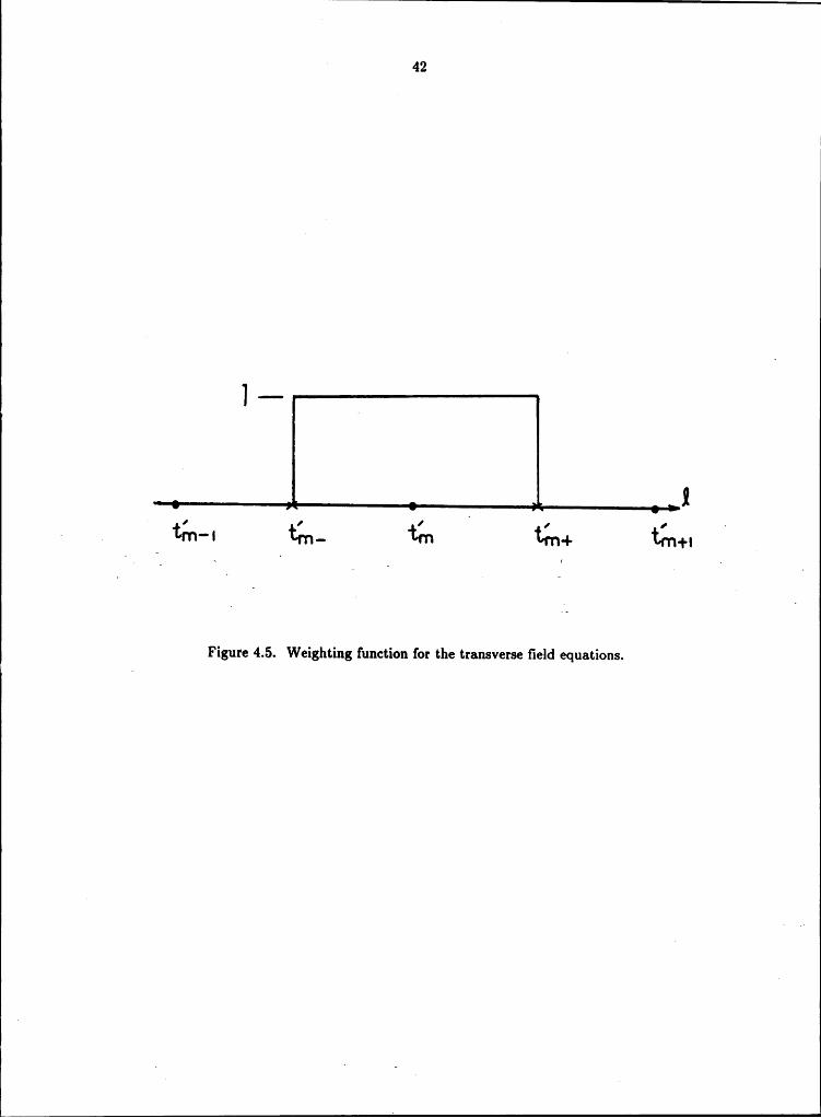
To enhance the accuracy of the results, pulse functions are used as the weightingfunctions for the transverse field equations (3.42) and (3.44) [5,318]. These pulse functions,which are centered at the grid point locations, may be stated mathematically as (see Fig. 4.5)

1 for tm_ S tS tm+‘ ‘Wm(t)=P„,(t)= , m=[1...N] (4.20) —0 elsewhere ·_.

where tm, is the midpoint of segment A€m_1 and tm+ is the midpoint of segment AE,~„.«

Using the current expansions (4.13 and 4.14) and the weighting function (4.20), the numerical·l

form of (3.42) may be written as (see Appendix C), \

N N-11. Z M:. (0%.. + ¤:..„) + Z M: (¤2... +Eä...)11:1 |1:1

+ äag #F2.,.+ J- Ffm.1.-1 JMZ1 1w<E

-11. Ü:. #6:%...+-% 6:....11:1 J‘·'€d J“·"cN k 2 k 2‘ —l- d —-L C = = 1...N . 4.21+n§1Jn (jwfä Hmn+ jwez Hmn) 0 1 m [ l ( )

By inspection, the numerical equivalent of (4.21) for the dual equaton (3.44) is given by

I

42

I 1 Ii A

1 1 «‘ tm"'l tm- im 1411+ tm-!-I

Figure 4.5. Weighting function for the transverse field equations.

43

the equation

· N t d C N z d C+Jk= E Ju (Dmu + Dmu) * E Ju (Emu +Emu)|1=1 I1=1

+ ETC Mh ="LFi—‘un+ **1- Finn..:1 wu; 1wuE

‘jk=..:1 Jwßä M42

+ §M;, if-u2„„+l=iug, :.1 „.:(. N) (.1·»·»)..:1 Jwßä M42 "’ °'

From Appendix C we note that the various “constant" terms (Bgm, Bgm, Bgm, Bgm,

Cgm, etc...) involve integrating a zeroth (or first) order Hankel function of the second kind.

These integrals are not tabulated and must be computed via numerical integration. The

technique of choice_ is [Simpson’s approach [13,110]. This numerical _integration ‘workhorse” isih

easy to implement and reasonablyi efficient [13,110]. Naturally, to obtain an] accurate1 ll

approximation of the integral, a substantial number of integrand (Hankel functions)evaluationsare

required. These evaluations are obtained by one of two techniques. If the magnitude of the

argument is less than 10.0, we use the power series form of the appropriate Hankel function

[2,959]; if the argument magnitude is greater than 10.0, we use the asymp-totic approximation

[2,962].

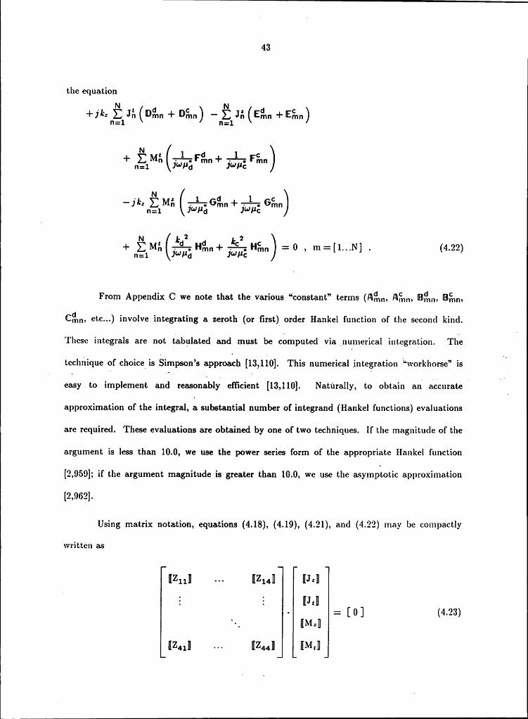
Using matrix notation, equations (4.18), (4.19), (4.21), and (4.22) may be compactly

written as

llZ11ll llZ14ll |lJ=ll

Ä E |IJ.ll• . : [0] (4.23)·. IIM=1l

llZ41]l |lZ4..I| llM.ll

l44

or, by definition,

pZ·I=0. (4.24)

In (4.23) each "element" [Zm„]| is an N x N matrix whose elements correspond to the

appropriate terms in equations (4.18) — (4.19). Each current “element" in (4.23) represents an

N xl matrix whose elements are the unknown expansion coefücients of the corresponding

current (see Eqs. 4.13 and 4.14). _

To have a non—trivial solution to (4.23) we require that the determinant of the Z matrix „vanish. Because of the approximate nature of the numerical implementation, a true zero of IZImay not exist. Rather, the “zeros” of IZI may only be local minima. To search for the

, minima we proceed as follows: given a particular waveguide geometry and the properties of the

dielect-ric and conductor,· we choose a value for the propagation constant lr,. Next, the elements

of [[Zm„]] are computed, followedi by theicomputation of IZI. We then vary kz in the ‘l

complex plane until a local minimum is found. The 2-dimensionali search algorithm for kg is 'I

based on the Powell’s n-dimensional minimization routine [13,294].

In Chapter 2 we stated that our goal was to develop a procedure which could determine

the allowed values of the propagation constant lr, for a waveguide structure. We now have that

teclmique. Any lc, satisfying Maxwell’s _equations causes a minimum in IZI. Finding all the

allowable propagation constants is usually not required. For any practical waveguide of

sufficient length, the behavior of a signal travelling along the guide is primarily influenced by

the "propagating modes”. These modes are characterized by a propagation constant having a

finite and positive real part (the other modes are generally characterized by a purely imaginary

propagation constant). Thus, we can instruct the search algorithm to minimize IZI by varying

ls, along the real axis. Once a minimum is found along the real axis, we locally vary lr; in the

complex plane until a local minimum is found.

45

4.4 SummaryIn this chapter we introduced an approximate technique that may be used to solve

integral equations. This technique, called the Method of Moments (MOM), reduces the integralequations to a set simultaneous linear equations, which may then be solved by a number of well-

known algorithms. Using this technique we developed a computer based algoritlnn to solve the

I waveguide problem. In the next chapter we present results for various waveguides.

Chapter 5

Computer Program Results

5.1 Introduction ·In this chapter we present the results of a computer program solution to the waveguide

problem developed in Chapters 3 and 4. We first present the results for lossless rectangular and

circular waveguides (Figs. 5.1 and 5.2). For these ideal cases, the propagation constant is

known exactly By comparing the results with the theoretical values, we may estimate the

validityu and accuracy of the computer code. As an additional verification, the results for a. ridged waveguide‘(Fig. are compared with_the approximations given by other authors (an

I I

4 exact solution is not known for the ridged waveguide). We conclude the chapter by presenting I

results for a lossy rectangular waveguide. The results are evaluated by comparing them with the

cstimations provided by perturbation theory.

5.2 Lossless Rectangular WaveguideThe first case we consider is the lossless 2 x lcm rectangular waveguide (Fig. 5.1). For

the cases studied in this section, we assume the dielectrics are air and the conductors are ideal.

In addition, all the materials are assumed to be nonmagnetic, pä = pa = po (we shall enforce

the nonmagnetic condition in Q the remaining problems in the thesis). For future reference, we

deline the propagation constant ask,

: ß — ja (5.1)

46

' I47

Qä

Figure 5.1. 2 x 1 cm rectangular waveguide. _

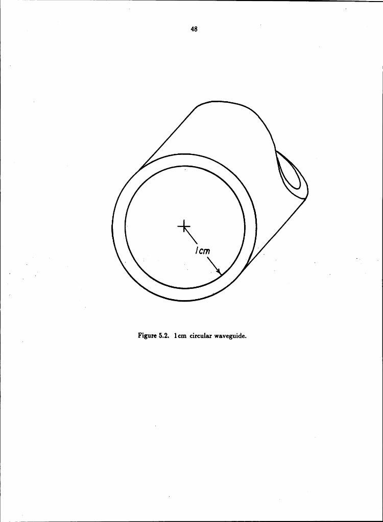
I_ 48 I I

49 i

*9i fg

‘

» 9 lcmg ‘+-/cm—~\ 3 Q. gi .. gi 9 3„ 2cm

i' ’ 4 A 3 ·

· Figure 5.3. Ridged waveguide.

?50

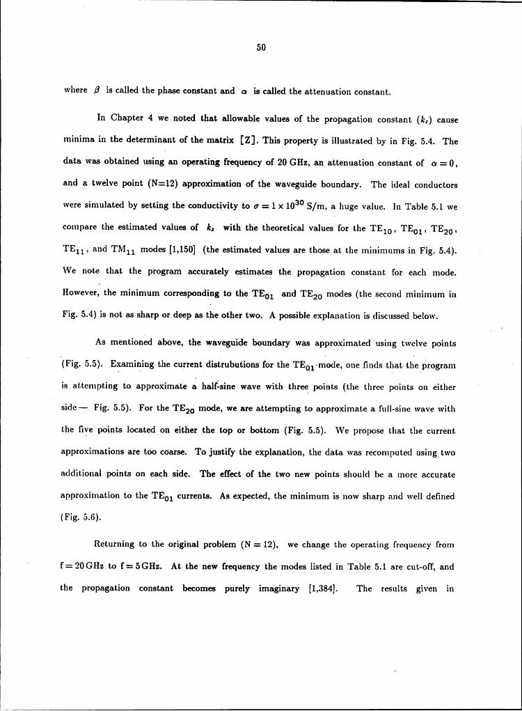
where ß is called the phase constant and cr is called the attenuation constant.

In Chapter 4 we noted that allowable values of the propagation constant (lr,) cause

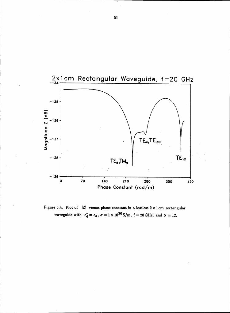
minima in the determinant of the matrix This property is illustrated by in Fig. 5.4. The

data was obtained using. an operating frequency of 20 GHz, an attenuation constant of cx = 0,

and a twelve point (N=12) approximation of the waveguide boundary. The ideal conductors

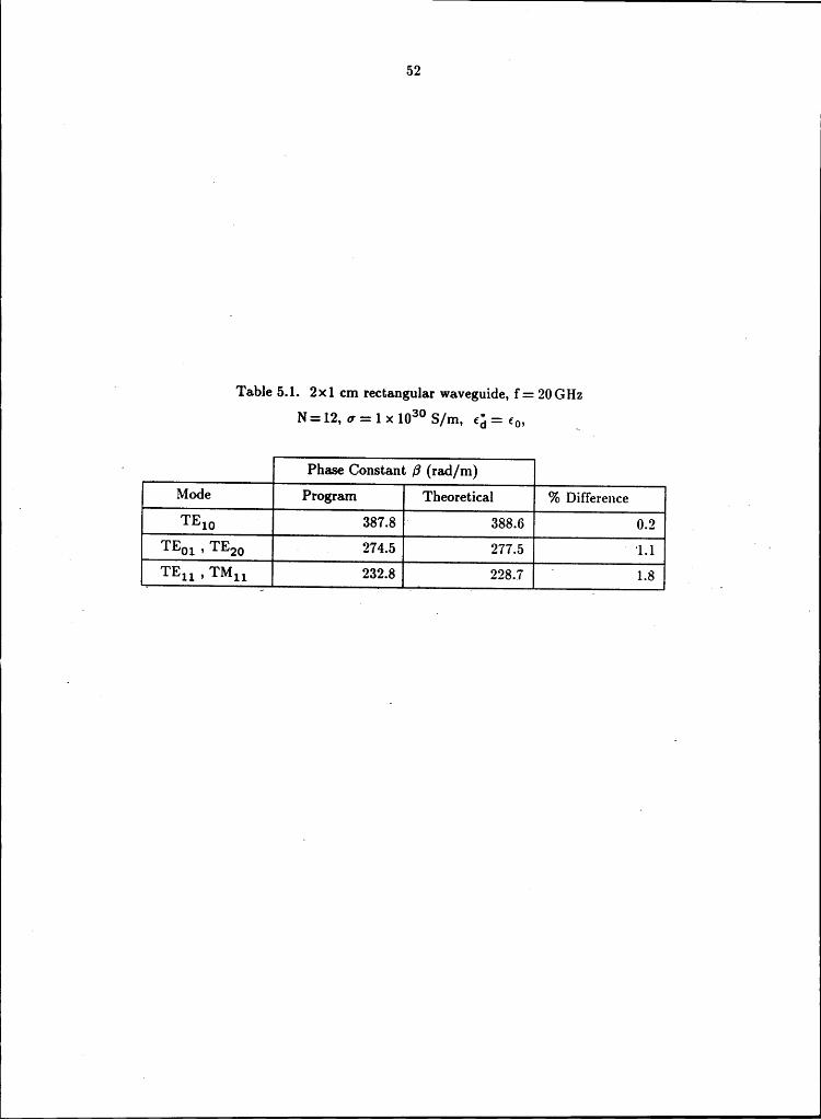
were simulated by setting the conductivity to 0 = 1 x1030 S/m, a huge value. In Table 5.1 we

compare the estimated values of k, with the theoretical values for the TE10, TEO1, TE20,TEN , and TMN modes [1,150] (the estimated values are those at the minimums in Fig. 5.4).We note that the program accurately estimates the propagation constant for each mode.

However; the minimum corraßponding to the TE01 and TE20 modes (the second minimum inFig. 5.4) is not as sharp or deep as the other two. A possible explanation is discussed below.

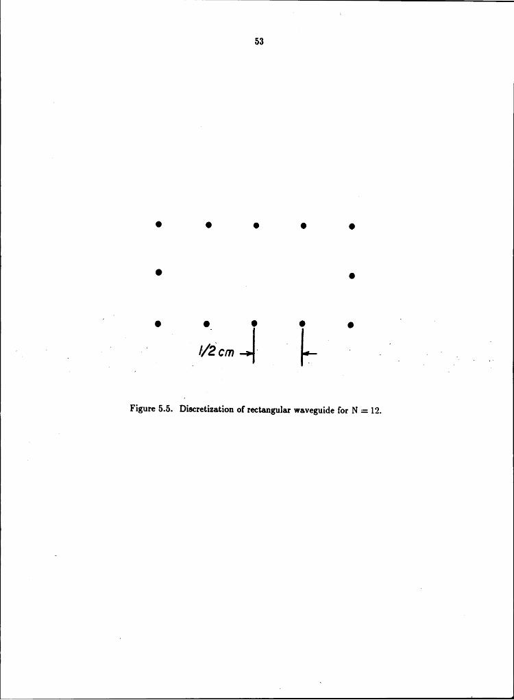
. As mentioned above, the waveguide boundary was approximated using tiwelve points . IE

I'(Fig. 5.5). Examining the current distrubutions for the TEQ1-mode, one finds that tlieprogram ‘

is attempting to approximate a halflsine wave with three points (the three points on either 'V

side- Fig. 5.5). For the TE20 mode, we are attempting to approximate alfull-sine wave with

the live points located on either the top or bottom (Fig. 5.5). We propose that the current

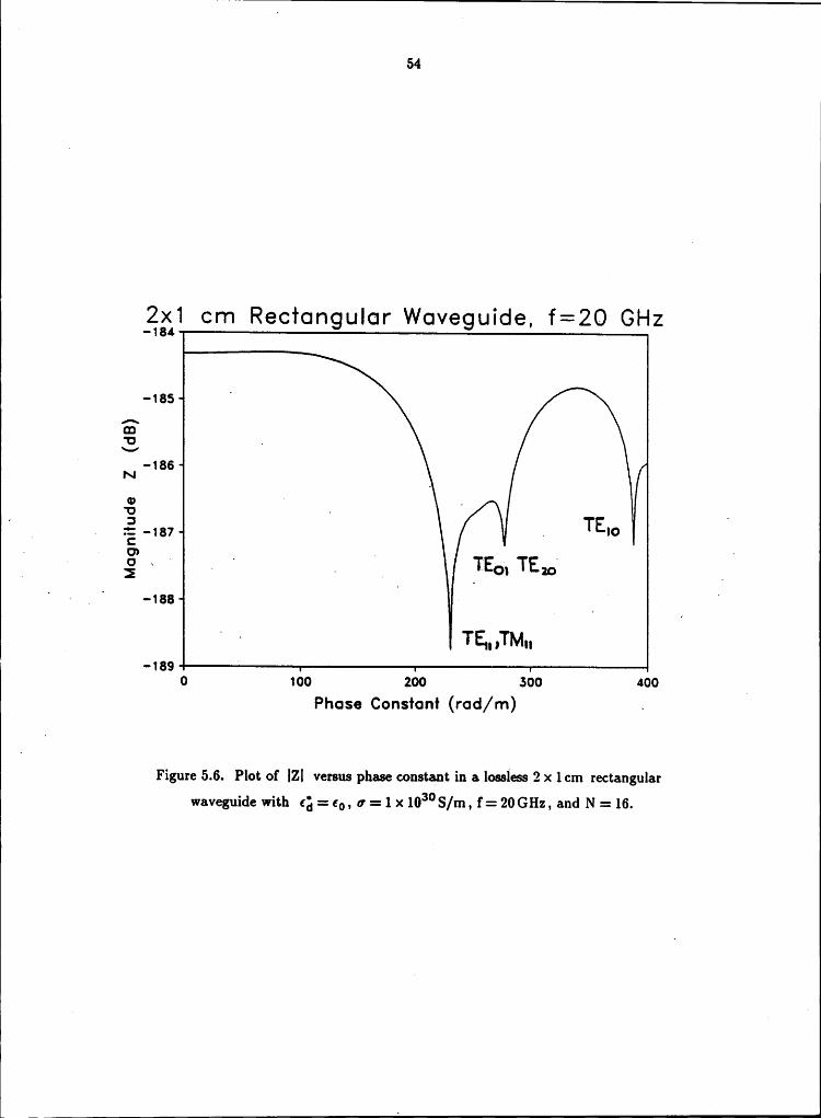
approximations are too coarse. To justify the explanation, the data was recomputed using two

additional points on each side. ~The effect of the two new points should be a more accurate

approximation to the TEO1 currents. As expected, the minimum is now sharp and well defined

(Fig. 5.6).

Returning to the original problem (N :12), we change the operating frequency from' f= 20GHz to f =5GHz. At the new frequency the modes listed in Table 5.1 are cut-off, and

the propagation constant becomes purely imaginary [1,384]. The results given in

V „ 51 1

%i<1 cm Recfangular Waveguide, f=2O GHz

-135·

E5UP V -136N

—

U A2gf'}? 1 TE„.„,TE„ .Q · .E . ,1 -138

ITE 1 F ‘ F 1

. · ° A TE•I;l·M•I ‘ Flo i

-1390 70 140 210 280 350 420

Phase Constant (rad/m)

i Figure 5.4. Plot of IZI versus phase constant in a lossless 2 x 1cm rectangularwaveguide with ca : 60, o· = 1 x 1030 S/m, f= 20 GHz, and N = 12.

52 1

2 Table 5.1. 2x1 cm rcctangular waveguide, f= 20GHzN=12,o·=1><103° S/m, 6;: 60, _

· Phase Constant ,6 (rad/m)Program Thcoretical % Differehce _ _I

TE10 2 387.8 · 388.6 0.2 .2 TEOI , TE20 2 „ 274.5 277.5 2 ’l.1 l 22222 · 22212 22**7 2 L8 2 .

53Z i

O O O O O

O l Q

( —O A O_ O O O O

A

Figure 5.5. Iiiscretization of rectangular waveguide for N = 12.

1U V 1

54

2:1 cm Rectangular Waveguide, f=2O GHz-1 4

-185 °

E?3 1

-186N 18 -‘ I 1 -2 -187 1 Tim 1

1 1 S -1 .' · 1

”-188

I· {

I'

_ ‘ TEMTMII-189 '

0 100 200 300 400 gPhase Constant (rad/m) 1

Figure 5.6. Plot of {ZI versus phase constant in a lossless 2 x 1cm rectangularwaveguide with ca = cu, 0* :1 x 103°S/m, f= 20 GHz, and N :16.

55

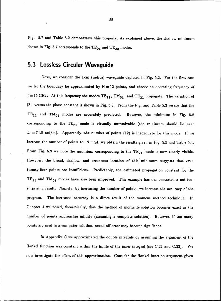
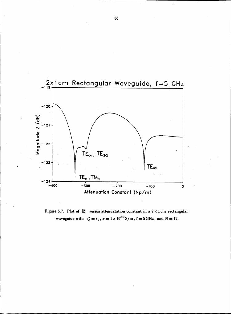
Fig. 5.7 and Table 5.2 demonstrate this property. As explained above, the shallow minimum

shown in Fig. 5.7 corresponds to the TEOI and TE20 modes.

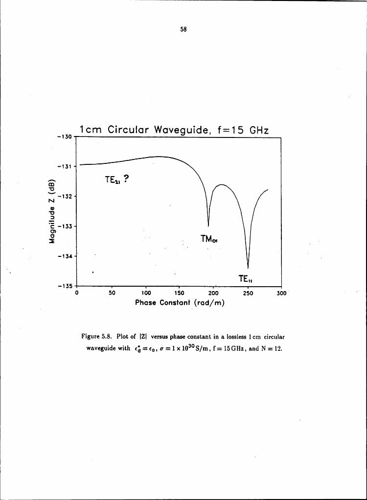
5.3 Lossless CircularWaveguideNext,we consider the 1cm (radius) waveguide depicted in Fig. 5.2. For the first case

we let the boundary be approximated by N :12 points, and choose an operating frequency of

~ f : I5 GHz. At this frequency the modes TE11, TM01 , and TE21 propagate. The variation ofIZI versus the phase constant is shown in Fig. 5.8. From the Fig. and Table 5.3 we see that the

TE11 and TM01 modes are accurately predicted. However, the minimum in Fig. 5.8corresponding to the TE21 mode is virtually unresolvable (the minimum should lie near

lr, :74.6 rad/m). Apparently,·the number of points (12) is inadequatc for this mode. If we _

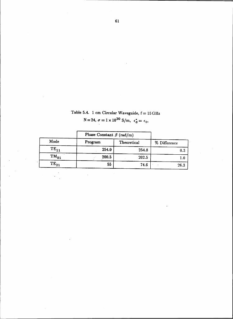
_ increase the number of points to N : 24, we obtain the results given in Fig. 5.9 and Table 5.4.

U ._ From Fig. 5.9 we note the minimum corresponding to the TE21 lmode is_ now clearly ivisible.’ llowevelr, the broad, shallow, and erroneous location of thisxn minimum suggests that even

twenty·four points are insufficient. Predictably, the estimated propagation constant for the

TE11 and TM01 modes have also been improved. This example has demonstrated a not-too-surprising result. Namely, by increasing the number of points, we increase the accuracy of the

program. The increased accuracy is a direct result of the moment method technique. In

Chapter 4 we noted, theoretically, that the method of moments solution becomes exact as the

number of points approaches infinity (assuming a complete solution). However, if too many

points are used in a computer solution, round-off error may become significant.

In Appendix C we approximated the double integrals by assuming the argument of the

Ilankel function was constant within the limits of the inner integral (see C.21 and C22). We

now investigate the effect of this approximation. Consider the Hankel function argument given

„ ~ 2 ' I

56

4%x1 cm Recfcmgulor Wcweguide, f=5 GHZ

-120

2 E3 -121N0‘¤2· °E -122 28’ 2 . 1 1

l 2-: ‘ 1 TEZQ _ 2 .H-123 - „ . 4

l I ·I

‘ — . · _ -l-Eng ‘4

TEN-124

-400 -300 -200 -100 0 ’

Afienuofion Constcnf (Np/m)

Figure 5.7. Plot of IZI versus attenuatation constant in a 2 x 1cm rectangularwaveguide with eg = 60, 6 =1x103°S/m, f= 5GHz, and N :12.

l

57

Table 5.2. 2x1 cm rectangular waveguide, f = 5GHz, N=12, 6 =1><103° S/m, 6; = 60,

‘ Attenuation Constant a (Np/m)Mode A Program 2 Theoretical % Difference

. TEI0 117.9 117.0IE .~ 926 2992

TE11 , TM11 335.2 . 0.2

° l58

30 1cm Circular Waveguide, 1:15 GHz-1

-151 1

16.. ?3

-152N

"U2'E -1332

.1 1.-

‘ .

_. -154 1 1 1 1 · . 1 .1

1-1550 50 100 150 200 250 300 1 ‘ °

Phase Consfanl (rad/m)

Figure 5.8. Plot of IZI versus phase constant in a lossless 1cm circularwaveguide with 6; = co, 6 =1x103°S/m, f= 15 GHz, and N :12.

III

59

Table 5.3. 1 cm circular waveguide, f = 15GHz "12:12, 0 =1x103° S/m, eg = 60,

A Phase Constant ßProgram Theoretical % DifferenceTE11 222-2 2-2so_I TM01 - 193.4 ” 202.5 21.5 ” - x

—‘TE21

H? I 74.6 ?\ ‘ · .

. l60

I 277 1 cm Circular Waveguide, f=15 GHz

-278I

E5 .-279N

013 TE=• _ 1°E -280 I3,

I _ V T MmE I 1

-2811

_l ·‘ _ I · i _

-282— ’ 0 50 100 ‘ 150 200 Z50 500Phase Conslani (rad/m)

I· Figure 5.9. Plot of IZI versus phase constant in a lossless 1cm circular

waveguide with 6; = 60, 0* =1><103°S/m, f=15GHz, and N = 24.

61

Table 5.4. 1 cm Circular Waveguide, f = 15 GHz1::24, o·=1x103° s/m, 6; = .0,Phase Constant ß (rad/m)Program Theoretical % Differcnce °

M1 MM MTEM YM

62

by equation (3.7),argument

: „]/:d2 — k,2 Ip — p'] . (5.2)

From (5.2) we have .

ö 1; = ,|1¤„*’-1:,*. (5.3)P — P l

As the frequency increases in a lossless waveguide, the propagation constant (lv, ) approaches themedium’s intrinsic propagation constant (kd) [1,384]. The result is that (5.3) becomes smallerand our approximations to the double integrals become better.

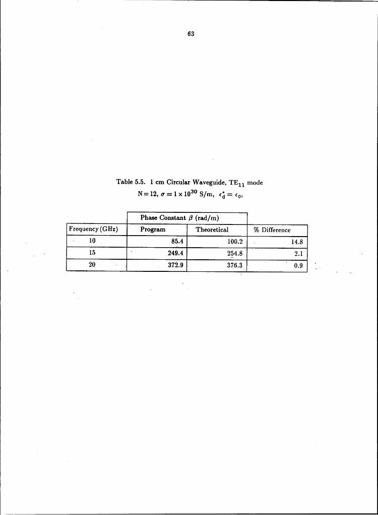
· In Table 5.5 we demonstrate the effect of frequency on the program. The estimatedphase constants correspond to the TE11· mode in a lossless circular waveguide. From the table

_[

we note the accuracy improves substantially with an _increase in the operating frequency. l ‘

5.4 Lossless Ridged WaveguideAn additional verification of the program was obtained by considering the ridged

waveguide shown in Fig. 5.3. An exact expression for the phase constant in this waveguide isnot known. For this reason, we evaluate our results by comparing with approximations givenby other authors.

For the present case, we choose an operating frequency of f: 15GHz and approximatethe boundary with N :20 points. The resulting plot is shown in Fig. 5.10. From the estimatedphase constants (minimum locations) we may compute the corresponding cut-off frequecies[1,384]. In Table 5.6 the estimated cut-off frequencies are compared with those given by [7,583].

4I

I 63

ITable 5.5. 1 cm Circular Waveguide, TE11 mode

N=12, o'=1><103o S/m, ca: 60,

Phase Constant ß (rad/m) V

Frequency (GHz) Program Theoretical % Differencc00 000-0 000I 0 00 0000 00 000 0 000-0 000-0 0

u64 0

I

Ridged Waveguide, f=15 GHz _.-227

-228 .

_ E5· 3 -229N01

'O2°E -2301 -O5 2 _ 1

V . · -231 0 .P ‘ ‘ . I

-2320 100 200 300 400

- Phase Constanl (rad/m)

Figure 5.10. Plot of IZI versus phase constant in a lossless ridgedwaveguide with 6; = 60, 0* =1x103°S/m, f= 15 GHz, and N = 20.

65

Table 5.6. Ridged Waveguide (Fig. 5.3), f=15GHz‘ N=20, o'=1x103° S/m, ca: 60,

Cut—off Frequency (GHz)ß Mode. Program Reference % Differcuce

. TE°°°' H 5.31 5.38 1,.37 . TE°"°"

‘ 11.95 ” " 11.78 1.4 ”

l66 „

[

5.5 Lossy Rectangular WaveguideIn this section loss is introduced into the rectangular waveguide problem depicted in

Fig. 5.1. The loss may result from conductor and/or dielectric materials. In this section wetreat each type of loss separately, and concentrate only ou the loss associated with the TEN

· mode.

The first problem we consider assumes the dielectric is air, the operating frequency is

f = 10 GHz, and the boundary is approximated by N = 12 points. Three different conductivities

were used, 0 :1 x 1030 S/m, 0 =1x107 S/m, and 0 =1x106 S/m . Recall in section 5.2

we simulated the lossless case by setting the conductivity to 0 = 1 x 1030 S/m. We repeat thiscase because in section 5.2 we were not looking for any loss, and only the real part of k, (ß) was

used to minimize the determinant IZI. We now desire to minimize IZI using both the real and

imaginary parts of k,. A . _ . ‘W

—

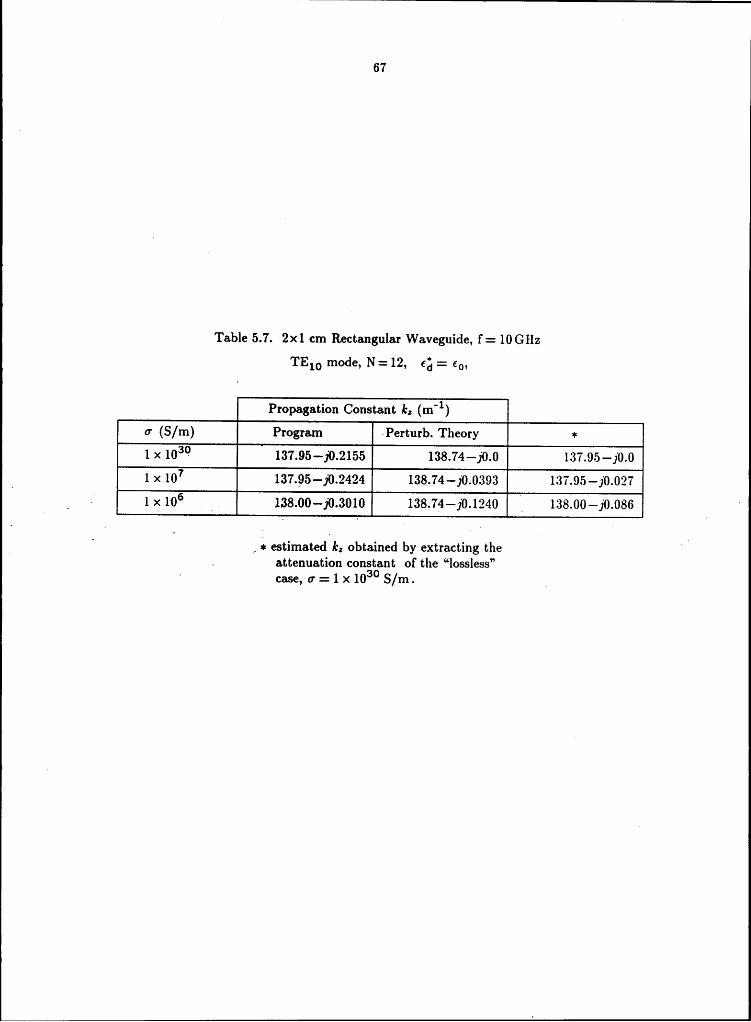
. . The results are shown in Table ‘5.7. For all three [conductivities the estimated _ I .attenuation constant grossly exceeds the values given by perturbation theory] [1,71].. If the~ _

attenuation constant of the “lossless” case (0:1x 1030 S/rn) is subtracted from the "lossy”

cases (0 =1x 107 S/m , and 0 =1x106 S/m), the results become much more reasonable (see

the last column in Table 5.7). We now attempt to justify the subtraction scheme.

For a conductivity of 0·=1x103°S/m the program should provide a vanishing

attenuation constant. The predicted “loss” at this conductivity may be an inherent loss

associtated with the discretization of the problem. For example, the loss may be viewed as a

"radiation” through the finite grid used to approximate the boundary; Although, we do not

claim the inherent loss is a radiation phenomenon, the analogy is provided as a convenient way

to view the loss. For a sufficiently small “radiation” loss, the overall attenuation constant

. 67

Table 5.7. 2x1 cm Rectangular Waveguide, f= 10GHzTEN mode, N: 12, cg : 60,

Propagation Constant ic, (m'1)0 (S/m) Program Perturb.Theory1

x 1030 137.95—j0.2155 138.74—j0.0 137.95 —j0.0V 1 x 107 . 137.95—j0.2424 138.74—j0.0393 137.95 —j0.027

_ Ö 1 x 1*06 V _ . 138.00·-j0.3010 138.74—j0.1240(V

138.00—j0.086 ‘

=l= estimatedukz obtained by extracting theV l 0

- attenuation coustant of the "lossless”‘ case, 0:1x1030 S/m. 0

68

should be given by

oz : oz, + cvother (5.4)where cr, is the attenuation constant due to the "radiation effect” and crother is theattenuation constant due to other effects (e.g. finite conductivity). The above concept is the

same technique where conductor and dielectric losses are added in a low-loss waveguide [1,74].

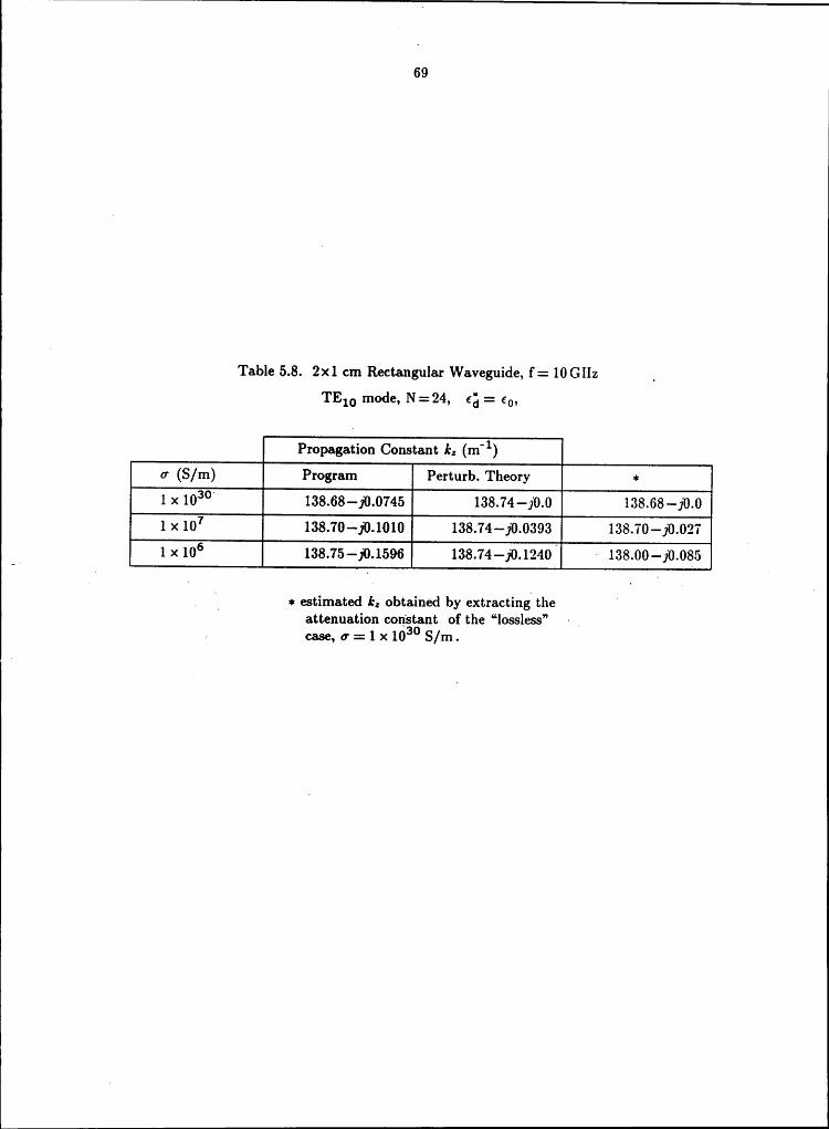
If we double the number of points in the current problem, we obtain the data given in

Table 5.8. As expected, the computed propagation constants were imp1·oved (see the second

column in Table 5.8). „ In particular, (we note the attenuation constant. corresponcling to

6 = 1><103° S/m has been dramatically reduced. Since the grid is more closely spaced, we

expect a reduced “ra.diation” effect. By comparing Tables 5.7 and 5.8 we observe an interesting

fcature—the “radiation-free” data (columns marked by =•=) are nearly the same in both cases.

This feature tends to validate the subtraction scheme (equation 5.4).

In section 5.3 we noted th.; performance of the program should improve as thefrequencyis

increased. We demonstrated this feature by [showing the improvement of the phase constantl

in the circular waveguide. We now idemonstrate the improvement in the attenuation constant.[

Consicler the same problem used to generate Table 5.7. If the frequency is increased to

f = 20 GHz, we obtain the data listed in Table 5.9. From the table we note the “ra.cliation-free” -propagation constants are now very close to the predictions given by perturbation theory.

We conclude this section by investigating dielectric loss. The problem we consider has

the following parameters: N: 12, f: 10GHz, and 6 =1><103o S/m. The dielectric

69

Table 5.8. 2x1 cm Rectangular Waveguide, f= 10 GI·Iz _€ä 60,

Propagation Constant k, (m°1)0* (S/m) Program Perturb.Theory1

X 1030. 138.68—j0.0745 138.74 —j0.0 138.68-—j0.01 X 107 138.70—j0.l010 138.74-j0.0393 138.70 -j0.027

g 1 X 106 138.75—j0.1596 138.74—j0.1‘240~ · l38.00—j0.085 ‘

_ ·_ =•· estimated k, obtained by extractingv the ‘ I

attenuation coristant of the “lossless” ~ V· case,0*=1X103o S/m.

70

Table 5.9. 2X1 cm Rectangular Waveguide, f= 20 GHz ·mÜd€, N: 12, €ä

= Öo,

Propagation Constant lv, (m'1)1

0* (S/m) Program Perturb. Theory

_

1 X 1030 388.3—}0.0766 388.6—j0.0000 288.6-]*0.00001 X 107 388.4—j0.1050

1388.6—j0.0290 388.4 —j0.0‘284 A

A 6 1 X 106 ,_ u 388,4—j0.1675 388.6 —j0.0917 · 388.4-j0.0909 l .

1 =•= estimated k,’obtaiped by extracting then ’ T A

attenuation constant of the "lossless”case, o· :1 X 1030 S/m.

‘ 71

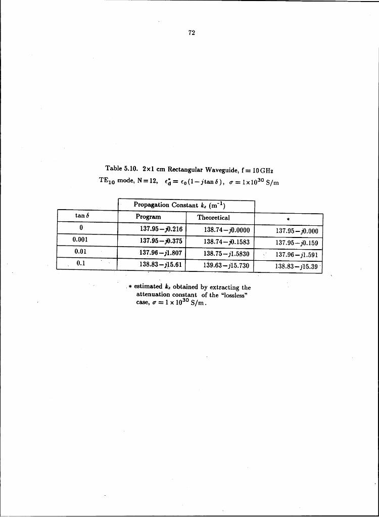
constant is chosen to be,

6ä=c0(1—jtan6) (5.5)

where tan6 is the loss tangent. In Table 5.10 we present TE10 loss data for several values oftan 6. From the “radiation-free" data in Table 5.10 we note the program accuractely estimatesdielectric losses.

5.6 Summary ‘In this chapter computer program results were presented for three waveguides——-the

rectangular, circular, and ridged waveguides. We initially verified the code by comparing thecomputed results with the theoretical values for the lossless cases. Losses were then introducedby considering a rectanglar waveguide having imperfect conductors and a lossy, dielectric.

. Investigation of the data led tola couple of important conclusions; First, we noted theprogram’s accuracy improvedlas the frequency increased. This fact is a direct result of theI _-approximations used in Appendix C. Second, the program appeared to have an inherent lossassociated with the discretization of problem. Specifically, we found that the loss estimates wereaccurate provided that the apparent loss of the "lossless case" was properly taken into account.

I

72

I ITable 5.10. 2x1 cm Rectangular Waveguide, f= 10 GHz

TE10 mode, N=12, 6; = c0(1—jtar16), 0* =1x1030 S/m

· Propagation Constant le, (m'1)tan 6 ProgramTheoreticalga 137.95-11).216 138.74-10.0000 137.95 -10.000

0.001 137.95—j0.375” 138.74—j0.1583 137.95—j0.159 10.01 · 137.96-j1.807 138.75—j1.5830 { 137.96 —j1.591

. _ 0.1 l ‘ l38.83——j15.61 139.63—j15.730 138.83——j15.39 ‘ .

- I. =•= estimatell le, obtained by extracting the 7

attenuation constant of the “lossless”, case,0:1x103° S/m.

I

Chapter 6 .

Summary and Conclusions

In this thesis a method has been presented which predicts the propagation constant in

E · microwave guiding structures. The method is valid for guides having an arbitrary cross-section.In addition, both conductor and dielectric losses are included in the development.

The problem was formulated using integral representations of the fields in terms of _„ vector potentials of the surface currents. The fields were evaluate at the boundaries separating

, i the various regions (e.g. the dieltric and Iconductpr regions). By imposing the continuity of 3tangential field components at the boundary, a set of coupled integral equations was derived.

The method of moments was used to reduce the set of coupled integral equations to a

linear matrix equation. The resulting equation had the form

‘ · [Z] · [1] = [6] (6-1)where [I] represented the amplitudes of the unknown currents and [Z] represented a

“constant" matrix which depended on the propagation constant k, (see Chapter 4).

To provide a nontrivial solution to (6.1), the propagation consta.nt lr, was varied (for a

given geometry) until a minimum of IZI was found. The computations were carried out usinga computer program, and results were presented for three waveguide types—the rectangular,

circular, and ridged waveguides. The program’s ability to predict the propagation constant in

both lossless and lossy waveguides was demonstrated.

73

l

74

Analysis of the program data led to several interesting points. First, not toosurprisingly, the estimated propagation constant improved when the number of boundary pointswas increased. The method of moments directly predicts this result (see chapter 4). Second,increasing the frequency improved the progra.m’s accuracy. This feature was a result of certainapproximations used in Appendix C. Finally, an inherent "radiation” loss associated with thediscrete nature of the moment method was observed. Even under a simulated lossless condition(0* = lx103O S/m), tl1e program predicted a finite attenuation constant. \\Vhen the coductivitywas set to reasonable values (e.g. 1x107 S/m), the program overestimatcd the loss. I·Iowever,

. once the “radiation l0ss” was extracted, the results were close to those given by perturbation

theory.

Presently, several extensions of the work are under considcration. First, an "impedance

V boundary condition” type formulation is being considered. With this type of formuIation,.theI rcsulting computations and matriciß are simpler. A second possiblity is extcnding the program

F

. 'I

to allow for multi·layered dielectric/conductor geometries. ”rx¤si1y,—a„c1usao„ of random, roughV

conducting surfaces is being considered as a possible dissertation topic. U _

References[1] Harrington, R. F., Time·Harmonic Electromagnetic Fields, McGraw-Hill Book Company,

New York, 1961.

[2] Gradshteyn, I. S., and I. M. Ryzhik, Table of Integrals, Series, and Products, AcademicPress Inc., Orlando, 1980.

[3] Spiegel, M. R., Vector Analysis, Schaum’s Outline Series, McGraw-Hill Book Company,New York, 1959.

[4] Spiegel, M. R., Mathematical Handbook, Schaum’s Outline Series, McGraw-Hill BookCompany, New York, 1968.

[5] Stutzman, W. L., and Gary A. Thiele, Antenna Theory and Design, John Wiley andSons, New York, 1981.

[6] Van Bladel, J. , Electromagnetic Fields, McGraw-Hill, New York, 1964.

[7] Harrington R. F., and B. E. Spielman, "Waveguides of Arbitrary Cross Section bySolution of a Nonlinear Integral Eigenvalue Equation,” IEEE Transactions on MicrowaveTheory and Techniques, Vol. MTT—20, September 1972.

_ [8] Fukai, I., and S. Kagami, ”Application of Boundary-Element _Method to-· · Electromagnetic Field Problems,” * IEEE Transactions on Microwave Theory and' _ Techniques, Vol. MTT·32, April 1984. ~ -i[9]

rDavies, J. B., and

iD.M. Syahkal, ”Accurate Solution of Microstrip and Coplanar '

Structures for Dispersion and for Dielectric and Conductor Losses," IEEE Transactions onMicrowave Theory and Techniques, Vol. MTT-27, July 1979.

[10] Mittra, R. (ed.), Computer Techniques for Electromagnetics, Hemisphere PublishingCorp., Washington, 1987.

[11] Taylor, E., and R. Mann, Advanced Calculus, John Wiley and Sons, Inc., New York,1983.

[12] Harrington, R. F., Field Computation by Moment Methods, Macmillan, New York, 1968.

[13] Press, W. H. , et. al, Numerical Recipes, The Art of Scientific Computing, CambridgeUniversity Press, New York, 1986. ~

[14] Mason, J. P., ”Cylindrical Bessel Functions for a Large Range of Complex Arguments,”‘ Computer Physics Communications, Vol. 30, January 1983.

[15] Davis, W. A., ”A Guide to Choosing Basis and Testing Functions in the Method ofMoments,” 1975 URSI Radio Science Meeting, Urbana, Ill, 3-5 June 1975.

[16] Collin, R. E., Antennas and Radiowave Propagation, McGraw-Hill Book Company, NewYork, 1985.

[ 75

I

Appendix A

I Derivation of Vector Potential Representations

Consider electromagnetic fields which exist in a homogeneous, isotropic region having acomplex permitivity 6'and a complex permeability p‘. Since Maxwell’s equations are linear, the

electromagnetic fields may be expressed as the sum of two fields — one field due to the electric

sources J and the other field due to the magnetic sources M. If we define

t- _ E E E°+_E"‘

(A.1)I

H E Hg + Hm A (A.2). I

and let the e fields be due to J and the m fields be due M, then we‘have [1,99]_Ä— T-VxE°=jr..«p*H‘i N

I(A.3)

VxH° = jw6*E° + J

V X Em = jw;1" Hm + M (A.5)

V X Hm = jw6"' Em . (A.6)

Taking the divergence of (A.3) and using the identity V~ (V x C) E 0, we have— V- (V x E°) E 0 = jw„*(V - H°) (A.?)

Gr-

V - H° = 0 . (A.s)From the identity V·(VxC) EO, we may define an auxillary vector quantity, the magnetic

t vector potential A, as He = V X A . (A.9)‘ Using (A.9), equation (A.3) may now be expressed as

Vx(E° +Jwß' A) = 0 . (A.10)

76

77

In view of the identity V x (VÖ) E 0, we may define an auxillary scalar function Öe (the scalar

electric potential) in the following manner:

-v<1»°=E°+j«„„*A. (A.11)Upon substituting (A.9) into (A.4) and employing the identity

VxVxCsV(V·C)——V2C, ·

we obtain

V(V·A) — V2A = jw6*E°

+JUsing(A.11),

V(V·A) — V2A = jw6*(— V<I>° —jwp" A) + J.u

(A.13)

ISince only the curl of A has been specified, we are free to chose its divergence. If we let

U

A- J

I IV·A= —jw6°Ö°,

1 " ' (A.l4)

· then (A.13) becomes l

V2A+k2A= —J (A.15)

where kg; w2p"‘6*. Substituting (A.15) into (A.12) yields,

= L - 2 A.16E° jw€,(V(V A) + k A). ( )

The m equations, (A.5) and (A.6), are duals of the e equations, Proceding in an analogous

manner, we obtain

Em: —VxF (A17)V2F+k2F= —M (A.18)

„ II

78- and

m _, 1 _ 2H — jam, (V(V F) +/6To

summarizc, equations (A.1) and (A.2) become

- - ..L . 2 ·E - vxv A) + 1 A) (A.20)

_ 1 _ 2H - VxA + jwp,,(V(V F) + I6 F) (A.21)with IV2A + 12A = —J 1 (A22)

‘ I· - V2F+k2F:.-—M

I I (A.23) _I I

and! I‘ k2 = w2p"'6". _· ”

I

Appendix B . I

Evaluation of Singular Integrals

In this appendix we evaluate the integrals developed in Chapter 3 at their singular

points. The first integral to be considered has the form

_ _ +6 (2)ÄPO ,ILP„ Ile [fp') ‘jl.{H¤ </=§»‘Ip—»'I> dl'- (B-1)

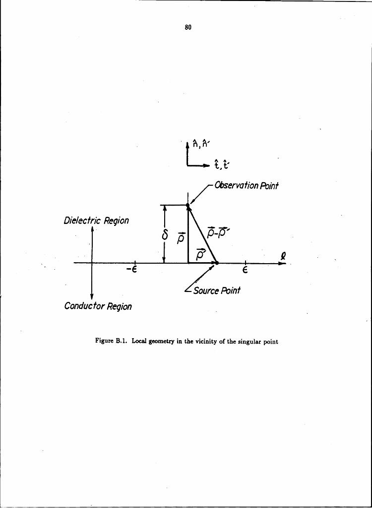
If we assume the contour Z (see figure B.1) is locally planar, the source location may be ·

. cxprcsscd as ‘ _ I ° I ’_ 'I 6 pl ¤ i"£'. (6.2)

The procedure in Chapter 3 also specified that the field point is to be placed at

p = +63 (6.2)From figure B.l we note that the argument of the Hankel function may be exprcssed as,

kS|p—p'I = kt! I<«·— ··'>2+ u- ¢'>2 (B-4)with

11:+6, 11':t:0.

Thus, the integral is equivalent to

. .l+‘1(2)d|z I2 r B61Lpo ölgnoü L6 I(t)H„ (/¤,, 6 +z )dt . ( .5)

79

so L

, ‘ A, Ail——» %, i: A

_ /-Observofion Poinf 4

Die/ecfric Region __ n. R ·• -[-i [ r„ Ö o p ,

· -6 6 ” r AL , Source Poinf LConducfor Region _ _

Figure B.1. Local geometry in the viciuity of the singular point

6 81

Given a sufficiently small argument, the series representation of the Grecn’s function (see[2,951]) may be compactly written as

(2) lL11., (11,,+

0[I1>—1>'I2!¤]1>—1>'I)} (B-6)

where C represents a constant term and O(]p—p']2ln[p—p'[) represents terms bounded by

order of magnitude [p—p'[2ln[p—p'[ . The current may be expanded in a Taylor series about‘ 1'=0 giving [4,110]

2I(t' = 1(o) + 1'-Öl] + L (1')2 LLZ! (615*,,:0

_ If we assume that the current is sumciently smooth within the interval 266, then (B.?) is °i I

equivalent toi

I(t') = 1(0) + O(t'), (13.6)and the integral (B.5) may be written as

- - _L_ +€1 d 2 I2€lLIPo 61%- 266 0(1 ))(C+ln[k„„[6 +1 )

+ 0{(62+ 1'2)1¤]62+ 1'2 dt, (13.9)

where the conditions 71 = + 6 , and nf = t = 0 have been enforced. Expanding the integrand

and using the O( notation, the integrand of (B.9) may be expressed as,

I(0)C + 1(0)111(11§,*,]6*’+ 1'2 )+ O(t')ln (11-$[62+ 1'2 (13.10)

82

Obviously, the integral involving I(0)C approachs zero as 6-+0. For sufficiently small

arguments, the third term of (B.10) is bounded by

I 0(1')1¤(112J62+ 1'2 (13.11)

As 6-+0 the right hand side) of (B.11) behaves as

.1. (gpc |11¤(6)| = 0 . (13.12)

Therefore, (B.9) may be evaluated by simply considering an integral of tl1e form

6 [ . .. 101) +6 .5I———2I2 1 .._ 4 _' _ . — flino ölino-WTIJ ln(k„ 6 +t )dt ~. _ (B.13)

This integral may be directly integrated giving

+€i- - [(0) 1 11 2 I2 1 -1611_q10I--T(1 ln(k,,„I6 +1 )—2t +26 1611 (6 ) (13.14)

—€

OT,

Eläno -@(6ln(lcg|6|)-26):0 . (B.15)

Therefore, the singular contribution of (B.1) is zero.

The next singular integral we need to consider is

- -+€ 1 1 ö (2) ,11 1 1 B 16(/wlß ßI)6[¢· (· )

83

By using (B.4), (B.6) and (B.8), integral (B.16) may be expressed as,

I· V6 d _12 I2gw timo 6210 -6 I(0)6n, C+ln(k,, ,I(n 11) + (t) )

+ OI:((1t — n')2+ )ln( ,I(n — n')2+ (t')2)d1’I

(B17)n = +6, n' = O I

which is equivalent to,A

- L. · · +6 .._—...6_ 1_ *211* KO) (6++5++0 6+2+0I6_€

‘6+ (tl)?

dt

+6 Ü- i ‘· · 2 1 2 16 +(t)))dt·

” Öbviously, the second integral of (B.18) vanishes as 6—» 0 . Integrating the first term yields, ·

KO) - - 6 -1 1'I+‘ _ !(0) 11 1: _ T(0)·T· (*3-**))

Another integral that must be evaluated has the form,

· · +6 1 1 6 (2) _d 1 1 ._ chlno I) dt . (B.20)

— Tl1e difference between (B.20) and (B.16) is the variable which is differentiated. The only

consequence of the new derivative is a negative sign (see B17). We conclude that (B.20)

reduces to1 — l(;l . (B.21)

84

The final integral we need to consider is€

6%),0 öli-rpo 6% I; KP') Hi2)(kg|P-P'|) dt' (3,22)

which, using (B.4), (B.6), and (B.8), is equivalent to· · _;Q +6 1 d I 2 1 222 61l_, (6**)+ °(‘ ))(°+‘“("·· 6

111'I . (3.26)t=0

Obviously, as 6 —> 0 , the term involving I(0)C contributes nothing to the integra].Integrating the remaining terms yields,

. . 6 , (t-t')cliißo ölßlblo 1(0) 6% ((t—t')ln(,|62+(t—t')2) + (1- 1') - öbäll

· +$ 6 O I1, 0{121„,|6*’+(1-1')2 I 1 2 1 ·(1=1.24) 1”

-6 , Ü: 0

Evaluating (B.24) at the limits of integration and taking the derivative gives,

. 1 -1+ — +12 Il—22

66 (6+02 IT——22— ———-—-— + ————-— + I 6 + 1+

2— 1 O 11:1 ,|62+ 1-6)2 . (B.25)+6+1+++1 6 ‘ l ...1Once (B.25) is evaluated at t=0, the first eight terms cancel and the last term is zero. We

conclude that the integral given by (B.22) is zero.

l

Appendix C

4 Numerical Form Derivation

In Chapter 4 we found that our numerical formulation led to the following form ofequation (3.41) — see equation (4.17):

t{T\+1 I, A

I I 2=(:)6(:-:„,--g) 4::0, m:[1...N] . (0.1)tm

where, 2

2 ii€r(:):][(Ö-@2-‘$E)§j 1w P,(:')dt'i

I {

E an' _ön’ 4:1 " A2"k

2- ::.2 lr 2- 1. 2 N+][ ä-;—G°+£+é-G° J2P :’ 4:’e( :4.., M. ..2. “ N )

N |#’ — :’|- #;Gd+%G° -‘?- J2 1--; P :' 4:'. 0.2A 2"( ) ( )

Tl1e left hand side of (C.1) is equivalent to evaluating (C.2) witl1 the field point located at the

middle of segment Aém. If we use this fact along with the fact that the current amplitudes,

85

Ä86

Jß, J and are constants, then (C.1) may be written as

p (I') dt!

~ 11 2- ki 1. 2- 1 2+ Jz][ L-;—Gd+i-GC P il dt',,;:1 n a( jwcd }w6C “( )

. N z' - tl_]kzn;1Jäi(äGd+ä§G°)%(1_%)P2¤(tI)d"= 0 (C-3)—Z

with m = [1...N]. Keep in mind that for a given m the field point is located at the midpoint .

of segment AZ,-,1.

Using the definition of P2n(t') (see equation 4.14), we may define the first integral in(C.3) as, U

i __ ·‘ 2 ‘ ·’ -A$‘„„ +Af„„ J _

i(C-4a)wheire,i J i J ’ U ‘ V

tf, C tl tlAd E 1 -— i- dt''“",::1 6n' An—1

Z+ [4+1 E 1 — —"“4* d1’ (c 4b)

tg67], AFI

andtf, C tl tlA2 .11'. mn ,:14 ön' An·1

l tiI+1 ' '@9Ü 1 --—‘"“ d' c 4+ 611, t • ( • C)

The subscript m in (C.4) reminds us that the observation point is located at the miclpoint of

the segment AZ",. Since the observation point is fixed for a given m, A\gm+M$m may be

evaluatcd via numerical integration. However, to numerically implcment. (C.4) in its present

_ 87

form would require an approximation of the derivative terms (e.g. finite difference). Another

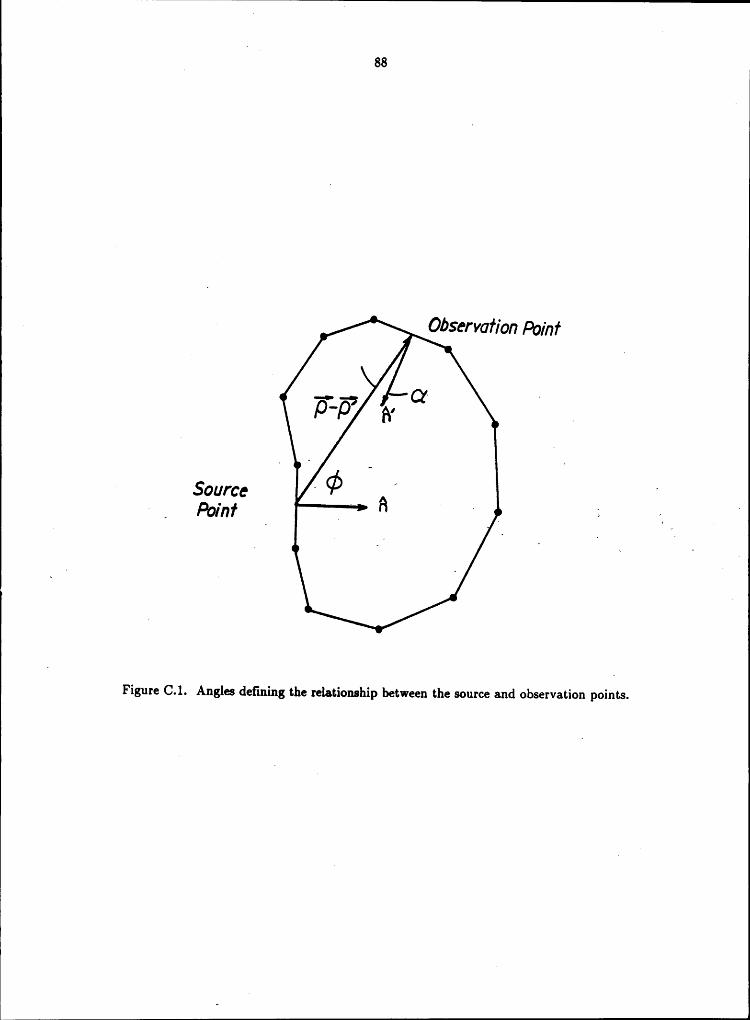
approach (the author’s choice) involves evaluating these derivates analytically. Consider thevector which defines the observation point with respect to the source point location (p—p’) —

Fig. C.1. If we define 45 as the the angle between the vector (p—p') and fil (the normal at

the source location), then from [5,369 ] we have

d kd (2)fg-% = T} cos,) 11, (ki |„-„'|) (0.6)or, l

( d kd A (2)@$-5 = ä (rw') H. (#3 iP—1>'i) (C-6)where,

1. fi ((:.1)”P‘P

In a similar manner, AI

c ),¢ 1; (2) ,. y , %% = ü (R-{J) 11, (ki, |„-„'|) ., „ . „ ((:.6) A

Now, consider the second integral of (C.3). From the definition of P,,(t') this integral is

equivalent toC

ll k 2_ k 2 Q'- Q[M-1 -L-%Gd+ [iii-GC dt' . (C.9)tg} Jwed JUJÖC

Wc define tl69,,,, E cd az' (C.10)

thand

z' _,_Bßn EV1 1 GC dt' . (C.11)rf.

Now, (C.9) may be written askd2'°k*2 d kc2"kz2 C

'i'

pF

ss S

. Observofion PoinfW »

Source ‘ ¢ Ai ' Ss _ Poinf S S ’ S @ q i

Figure C.1. Angles deüning the relationship between the source and observation points.

89

From the definition of P2n(t') the third integral of (C.3) becomes

tf, tr tr ‘-L(;d+-L(;¢ Ä 1- L

tn-1 ywcä jwcß ’@1' And

R‘i1+1 6

1’-1’+]R -l-G*'+#-cf -7 1- -J dd (c.16)tn ywcd ywcc 61 An

which is equivalent to

-J-6** + #6** C.14 RITII1 ( )

I whereR

1 . ~ _‘

__ · R1 R

RR ·R 1R¤RRt!‘iR

1a:«R°R tf‘+‘1R—1R‘Rd’zRR‘”RRR'_ · — » C„,„=-"[_ -X+G dt ——[ E-G dt < · ‘· g(C.15a) _, _ . .

and ' ’7 _ -

” 41 1 t|2+1 1 If cfm, E I E- cf az' - I Tof dt . (0.1611)‘ R th-1 ml th n

Using (C.4), (C.12), and (C.14), equation (C.3) may be expressed as

N 1 d c N z kd2‘k=2 d kc2—kz2 cAmn) Bum

#-6** +#c** -0 m=[1 N} (C16).7Zn-!} I1 jwcä ITII1 jwfé |'I1|1 * 1

V90

If we substitute the current expansions (equations 4.13 and 4.14) into the integralequation (3.42) we obtain

. N z' - z'—Ik, Hr? +r?)11;1M:„ (1

E N I I+ ön + ön )n§1 dt

Gd (1- Lg ) 1>2„(I') I1I'_ · _Ö_ d 1 C N z I I

U I

, 2 2 N I_ I+][(%1Gd+;l1%G°)EJf„(l—q)P2„(t')(/I'·/I)dt'=0. 1 (C.17)d c n=1 ·. E _ 1 .

. , — · ‘MultipIying (C.17) by the weight function (4.20) and integrating yields,_ I ” ., C I‘ 1 — tm+ 1.

1 §(@) dt =_0, m=[1...N] (C.18) 1 «tm•

where §(t) is defined as ”

gu); -IIC. ][(r? +r?)n;1M;,(1-d

c N+ }<%—+%>Z MrP··<I'> IIG fl:].

Q 1 CI 1 C Q"„ _l¢'—II€l I IA Pznu ) dt

__ · 1 d 1 C N z I IJ„ P„(t )dt

2 3 N I_ I+][(%é—;Gd+%G°)ZJ§,<1—@)P2„(t')(/I'-,I)dt'. (C.19)d C TI:].E

I

91

Recall that in Chapter 4 we defined *1- and *1+ as the midpoints of S€glTlClIES AEm_1 andAäm, respectively.

The first term of (C.18) is equivalent to _

N t' t' 1_ 1-1*1, ZM}, V‘V (0*1+0°) 1- %i (1’§'-’£)111'd1**=1 t:T'I· ##1 ***1Z, t' 1 1+im

tn-1 n-1

t' t'+1 ~ 1_ 1+I mIn##1-tlil " .tl

+t’+1

I I , .+V‘

V .‘ (0.20)1 I An«eii

_ n- Since lt and ii, are constant within the limits of each _double integral, tl1e dot products may ' J_ be taken outside tl1e integrations. Interchanging the order of integration yields,

i

N 1' 1_ 1 z'MA1-11:11:1-1 1*1-1 dmtl I_ I tl

++($#-·/1i„,)·V‘ (1- %.#)1*** (0*1+0°)111111'

1:1-1 "'1 tint’+1

I I tl+(fi,# -’£„,-)V(1-1f," zf,1-

+1 - + .(1- (0.21)## " tif!where tl1e following dot product notation has been adopted: the subscripts 11, a11d 111, referto u11it vectors at segment locations A£n_1 and A€m_1 , respectively; tl1e subscripts ll and 111

92

refer to the unit vectors located at segments Aln and Alm, respectively. To numericallyevaluate (C.21) in its present form requires four double integrations — a very time consumingprocess. To remedy this problem, we approximate the inner integral. Specifically, we make thecourse approximation that the integrand is relatively constant over the interval of integration.This “constant” value is taken to be the integrand evaluated at the midpoint of the the limits ofintegration. When the source point and field point are in the same segment (called the self-

'g patch segment), the integrand variw dramatically (in fact, the Hanke] has a singularity in thissegment). However, since the dot product term is zero, our assumption is not invalidated. Theapproximate form of (C.21) becomes

r*1kzZ Mw (“w·' im-li 1‘ %‘ "IÄL (G 2'G )w¤-/2 dtI1:]. t:|_1 I1-].

·I l

M ^ 2* ' #:1- I, Am d cI rl

(G +G dt - _·

_ ” 1 n·1 ' I” _ .

. +(11„-¤„,-)I,_ 1-%* (G +G°)„„_/2;:1‘- n .

G^· 2 2*+* 1 "‘ ‘i· Am Gd GC dd (G ww)+(¤n ' I11) 1,

“T T + m+/2 ""'n .

where m+/2 (or m-/2) reminds us that the observation point is to located at midway

between the points im and t:“+ (or midway between tin- and tin). If wc let gm+Dgmrepresent the terms inside the bracket, then (C.22) may be written as

- N z d cI1:

The last term of (C.18) has the same form as the first term. If we follow the above procedure

and make the same approximations, this term may be written asN k 2 k 2Ji Hd

+ HCmn Jwfc mn ( )

93

where

**1-- jr (@1*)-.-1- 1-'”tn-1 n-1

^1 ^id‘

ih- il Am d 1tn·1

^1 ^ #*+1l

¢' ··— th Am-1 d 1U + (1,, -1;,,,-) L, 1- (G )m_/2 dt .I']

(6; )m+/2 dt . (6:.26)~ in ' .

The definition for Hfm, is the same as (C.25) with GC substituted for Gd.

The second term of (C.18) is equivalent to

1 1 1 ,,2, ·* ,, ft, (6;:+*6;*) ~ 2 - _ 1H1- fl 1I I

i ·—t:Tl+ th-}-1

i d cU

i+I I (Ö£+@G-) 11/111} . (6:.26)ön Ön

To reduce (C.26) to a single ihtegral, we first reverse the order of integration and assume theintegrand is constant over the interval of integration. Again, we take the “constant” value to bethe integrand evaluated at the midpoint of the limits. This process givesN ‘:*+1 66;*1 66;° 1,,;,M" {LL (W"? FF)m·/2 dt

t:"l'1 öGd ÖGC dll (C -77)+ ,, (67+ wr)-+12 ·—fl

where the notation has been defined in (C.22). From (C.5) we have6

- = -% cos 01 H§2)(kg |p—p’|) (C.28)

A94

where 0 is the angle between fl and the vector from the observation point to the source point(p'—p ) —see Fig. C.1. Using the previous notation (see C.7), we have

d kd ^ (2)= -7l*L(11·«’ä)i-1, (kg |p-p'|) . y (0.29)

The first order Hanke] function exhibits a singularity in the self-patch segment. Again, the l’ singularity is nullified by a dot product (see C.29). We define the bracketed terms in (C.27) as

Egm ‘l' EnmSwing'

N z d CE M„(Em„ + Emn) . (C.30)|'I=1

‘ The third term in (C.18) has the form _

I. _ N Gd —__ I1:1 t:n_ t tL_1 Jwfd _J‘·•'€c ät ’

Once the inner integral of (C.31) is calculated, we are left with a function of t. Forconvenience, let this function be defined Next, f(t) is differentiated and thenintegrated from tfn- to t:n+ The above operations are equivalent to finding f( t(~„.) — _/( tfuThus, (C.31) becomes,

N #*+1 ö lt, " tfwl 1 d d* ...)m+(G1

c _ c I+ iwf; |:(G )m+(Gwhere

the notation m+ (or m-) signifies that the observation point is to be located at 4,,+

95

(or tfn Carrying out the derivatives yields,

gr L VA L [(0*1) -(0**)„=1" iwéä ,:1_1 An•11 cl d

1I"Iz' A

· .L " ; ¤ - ¤ 11 ^n·1 ÜG )"‘+(Gn•

» *:1+1 · L1- I1, K1. [(0**),,,+ - (0**),,,.] 11/)} . (0.64)fl

We define the first two integrals in (C.34) as Fgm , and the remaining two are defined asFgm. Now, (C.34) may be written as · q

1* Lrd L IFC 1 ‘ 0.661 . 1 1 ng]: n(Jw€d mn+ JwfcmnThe

fourth term in (C.18) is equivalent to . 1

~ *1+ 6 **1+1 6 1 1—jk, dt dt . (C.36)

n=1Followingthe same steps as above,

*1 $*;.1+ 1 (0*1) )11/J zI1:1 n j""Ü zf, m+ m-

tl.; "*'1 gc - 0** 11/ C.37+,,,,%:1 (1

‘96

l

If we define 6%,, as the first integral in (C.37) and 6%,, as the second, then (C.37) can bewritten as

N_ · 1 d 1 cJh: n§1JÄ(jw€ä Gmn + jule; Gmn ((7-38)

Using (C.23), (C.24), (C.30), (C.35), and (C.38), equation (C.18) may be written as

· N t d 7C N z d C‘Jk= E Mn (Dmn + Dmn) + E Mn (Emn + Emn)n:1 n=1 —

+ §jJ:, 4%,,+ 4 Fä,,,, ,,:1 M; ME .—jk, gr 4 62,,, + 462,,,,,:1 " JM; Jweé · y ·_

Q ’ ~. h1”7¤‘( hkcz g 7 °· + io', m=[1...N]•H: