EE 460 – Introduction to Communication Systems MATLAB Tutorial #4

Waveform and Spectrum of an AM Signal This tutorial provides examples of using MATLAB to graph the waveform and spectrum of an

AM signal. These are applications of commands introduced in previous tutorials.

Waveform of an AM Signal

Assume that a baseband signal:

x(t) = cos(2π100t) + cos(2π500t)

is used to modulate a 1 volt, 5 KHz carrier signal. The highest frequency (500) has a period of

0.002 seconds. If we want at least 10 points per cycle we need to sample points every 0.0002

seconds. The baseband signal can be plotted using:

>> clear >> N=250; >> ts=.0002; >> t=[0:N]*ts; >> x=cos(2*pi*100*t)+cos(2*pi*500*t); >> plot(t,x)

The 250 points gives us 5 cycles of the composite waveform. The general form of an AM signal

is:

xAM (t) = Ac 1+ mxN (t)[ ]cos2π fct

where xN(t) is a normalized version of the baseband signal. In order to normalize x(t) we need to

divide by its maximum value or in MATLAB:

>> xN=x./max(abs(x)); >> plot(t,xN)

Note that the normalized baseband signal now goes between +/- one. If we assume a modulation

index of m = 0.5, the resulting AM signal is of the form:

xAM (t) = Ac 1+ mxN (t)[ ]cos2π fct

= 1+ 0.5xN (t){ }cos(2π5000t)

or in MATLAB:

>> xam=(1+0.5*xN).*cos(2*pi*5000*t); >> plot(t,xam)

This does not appear to be an AM waveform. It looks more like the baseband signal. Where is

the error? Consider the frequency of the carrier frequency, 5000 Hz. A 5000 Hz signal has a

period of T = 1/5000 = 0.0002 seconds. This is the same as the sampling rate that was applied to

the baseband and modulated signal. Thus, we are only plotting ONE point per cycle of the

carrier frequency and the thus the plot does not correctly show the detail of the modulated

waveform. In general we want to have at least 10 points per cycle of the highest frequency

component to show adequate detail in a waveform plot. In this case we should be calculating

points every 0.00002 seconds. Thus, repeating the MATLAB code with this new sampling

interval:

>> N=2500; >> ts=.00002; >> t=[0:N-1]*ts; >> x=cos(2*pi*100*t)+cos(2*pi*500*t); >> xN=x./max(abs(x)); >> xam=(1+0.5*xN).*cos(2*pi*5000*t); >> plot(t,xam)

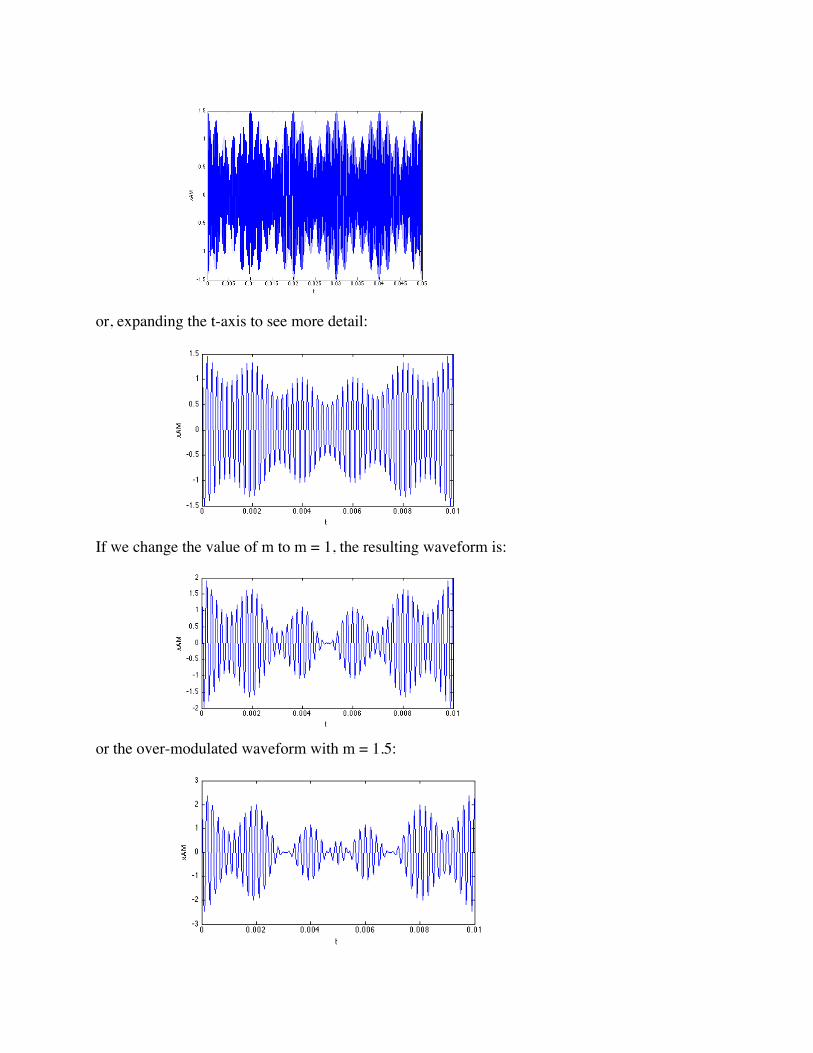
or, expanding the t-axis to see more detail:

If we change the value of m to m = 1, the resulting waveform is:

or the over-modulated waveform with m = 1.5:

Introduction to Simulink

Simulink is a companion program to MATLAB and is included with the student version. It is an

interactive system for simulating linear and nonlinear dynamic systems. It is a graphical mouse-

driven program that allows you to model a system by drawing a block diagram on the screen and

manipulating it dynamically. It can work with linear, nonlinear, continuous time, discrete time,

multivariable, and multirate systems.

Getting Started with Simulink

In this section we will illustrate a very simple use of Simulink to display a sine wave in the time

domain.

1. Open MATLAB and in the command window, type: simulink at the prompt.

2. After a few seconds Simulink will open and the Simulink Library Browser will open as

shown in figure 1. It is important to note that the list of libraries may be different on your

computer. The libraries are a function of the toolboxes that you have installed.

Figure 1. Simulink Library Browser

3. Click on the New Model icon in the Library Browser window. An additional window will

open. This is where you will build your Simulink models.

4. Click on the “+” sign next to “Simulink” in the Library Browser. A list of sub-libraries will

appear including Continuous, Discrete, etc. These sub-libraries contain the most common

Simulink blocks.

5. Click once on the “Sources” sub-library. You should see a listing of blocks as shown in the

right column of figure 2.

Figure 2. Source Blocks in the Simulink Library

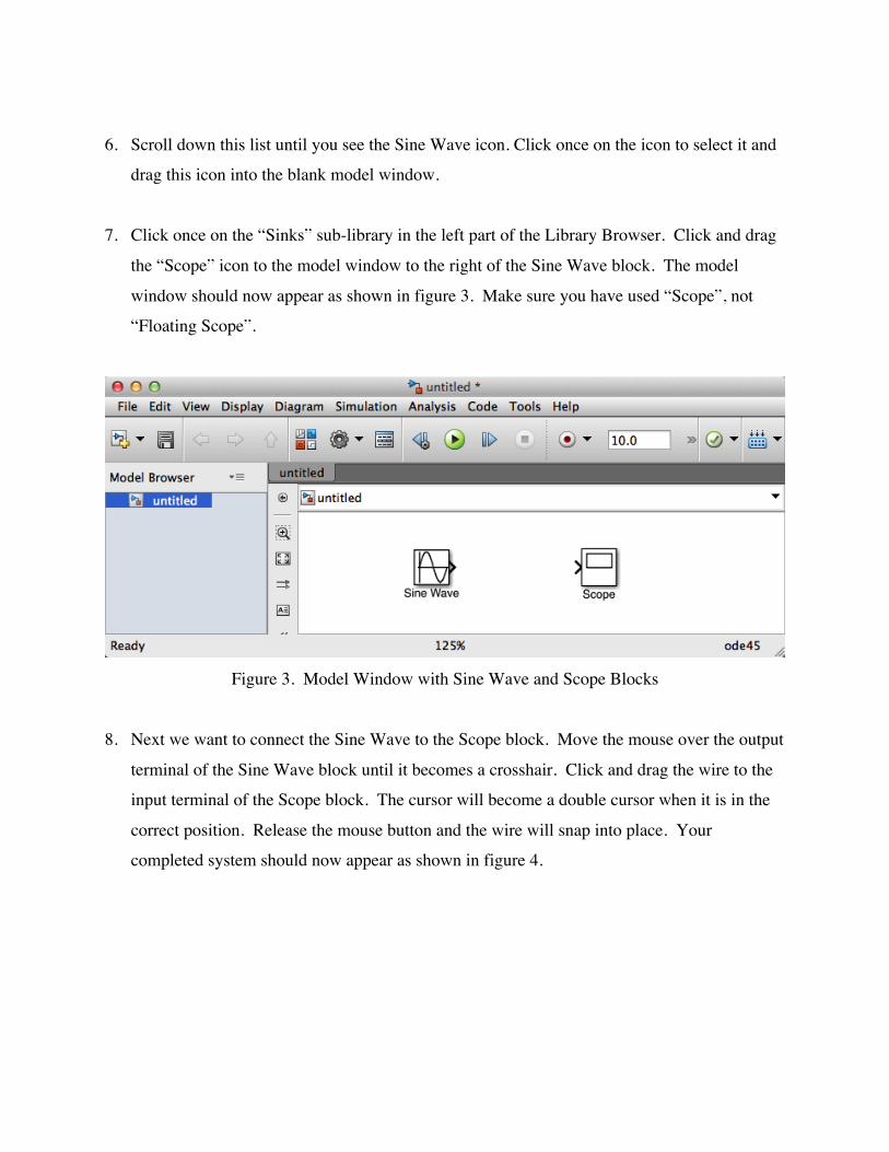
6. Scroll down this list until you see the Sine Wave icon. Click once on the icon to select it and

drag this icon into the blank model window.

7. Click once on the “Sinks” sub-library in the left part of the Library Browser. Click and drag

the “Scope” icon to the model window to the right of the Sine Wave block. The model

window should now appear as shown in figure 3. Make sure you have used “Scope”, not

“Floating Scope”.

Figure 3. Model Window with Sine Wave and Scope Blocks

8. Next we want to connect the Sine Wave to the Scope block. Move the mouse over the output

terminal of the Sine Wave block until it becomes a crosshair. Click and drag the wire to the

input terminal of the Scope block. The cursor will become a double cursor when it is in the

correct position. Release the mouse button and the wire will snap into place. Your

completed system should now appear as shown in figure 4.

Figure 4. Completed System for Viewing Sine Wave

9. In the model window select Run button. You will hear a beep when the simulation is

complete. Double click on the Scope icon and it will open and display the output of the sine

wave block. Try clicking on the Autoscale icon in the Scope window. This should cause the

axes to readjust as shown in figure 5

Figure 5. Scope Display

10. Note that the period of the sine wave is just over six. What frequency does this correspond

to? Return to the model window and double click on the Sine Wave block. The Sine Wave

parameters window will open as shown in figure 6.

Figure 6. Sine Wave Block Parameters

11. The frequency was set to 1 rad/sec. Any of the parameters shown can be altered to change

the sine wave. Change the entry in the frequency parameter to: 2*pi*10. This is a 10 Hz

sine wave. Click OK and re-simulate. Use the Autoscale icon to expand the scope display.

What do you observe? The sine wave should NOT be displayed properly. This is because at

this higher frequency the sampling rate has not been set high enough.

12. Return to the model window and select the Model Configuration Parameters icon. The Stop

Time for the simulation defaults to 10. Change it to 1, click OK, and re-run the simulation.

You should now be able to properly view the sine wave on the scope. Use the binoculars to

expand the display. Verify that the period of each cycle is one 0.1 second as you expect for a

10 Hz wave.

13. Another method for modifying the display is to specify the step size. Return to the model

window and select the Model Configuration Parameters icon again. Note that the Solver

Type defaults to “variable-step”. Change the Solver Type to “fixed step” and then enter the

value 0.001 into the Fixed Step Size entry. Click OK and run the simulation once again.

Note that the display is now smooth.

Viewing the Spectrum of a Signal in Simulink

1. Return to the Library Browser and open the “DSP System Toolbox. Click on the “Sinks”

sub-library and note a block titled “Spectrum Analyzer.”

2. Create a new model as shown below in figure 10. The settings on the sine wave block should

remain as they were set above. This configuration should cause the sine wave to be

displayed on both the scope (time-domain) and the Spectrum Analyzer (frequency-domain).

Figure 10. Spectrum Analyzer Sink

3. The Spectrum Analyzer will display the FFT of its input. Run the simulation. The Spectrum

Analyzer will open but an error message will be displayed. Note that a different Sine Wave

source must be used with the Spectrum Analyzer and other blocks that require discrete signal

types.

4. Replace the Sine Wave block with the Sine Wave block found in the DSP System Toolbox,

Sources sub-library. Double click on the new sine wave source block. Change the frequency

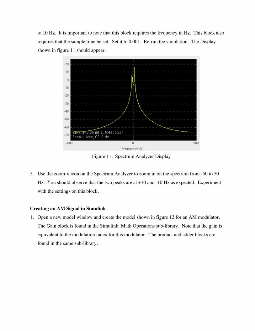
to 10 Hz. It is important to note that this block requires the frequency in Hz. This block also

requires that the sample time be set. Set it to 0.001. Re-run the simulation. The Display

shown in figure 11 should appear.

Figure 11. Spectrum Analyzer Display

5. Use the zoom-x icon on the Spectrum Analyzer to zoom in on the spectrum from -50 to 50

Hz. You should observe that the two peaks are at +10 and -10 Hz as expected. Experiment

with the settings on this block.

Creating an AM Signal in Simulink

1. Open a new model window and create the model shown in figure 12 for an AM modulator.

The Gain block is found in the Simulink: Math Operations sub-library. Note that the gain is

equivalent to the modulation index for this modulator. The product and adder blocks are

found in the same sub-library.

Figure 12. AM Modulator

2. This modulator is configured so that the top sine wave represents the baseband signal and the

bottom sine wave represents the carrier. Set the baseband frequency to 200 Hz and the

carrier frequency to 2000 Hz. Leave both amplitudes at the default value of 1. Set the

sample time of both sine wave blocks to .05mS. Initially set the modulation index to 1 (gain

of gain block).

3. Open the Configuration Parameters window. Set the simulation stop time to .02. Since the

period of the baseband signal is .005, this will cause 4 cycles of the baseband signal to be

displayed. Set Type to Fixed Step and the Fixed step size to 0.05mS. Close the window and

run the simulation.

4. The scope should display the AM waveform that you expect. Recall that m = 1. The

Spectrum Analyzer should display the expected spectrum. You may need to use the zoom

feature.

5. Experiment with the various parameters: m, baseband frequency, carrier frequency and

confirm that the results are as you expect. This will help you have a better understanding of

how to set up the simulation in future problems.

Importing the Baseband Signal into Simulink In some cases you will want to generate a signal in the MATLAB command window and import

that signal into your Simulink model. This section illustrates the procedure for importing a

baseband signal into the AM modulator created above.

1. Generate an AM waveform in the MATLAB command window using the following

commands:

>> clear >> ts=.00005; >> N=400; >> t=[0:N-1]*ts; >> x=cos(2*pi*100*t)+cos(2*pi*500*t); 2. Remove the upper sine wave generator from the simulink model created in the previous

example.

3. Drag the “Signal from Workspace” block from the DSP System Toolbox, Sources library

into the model window.

4. Double click on the Signal from Workspace block and enter the values as shown in figure 13.

Figure 13. Parameters for Signal from Workspace Block

5. Select the Configuration Parameters icon from the model window and change the Stop time

to 0.02. Use Type: Click OK and run the simulation. Double click on the Scope block to

view its display. Click the Autoscale to expand the display and confirm that it corresponds to

your x(t) as shown in figure 14.

Figure 14. AM Signal on Scope

6. Check to make sure that the spectrum is what you expect for your imported baseband signal.