wavelets in scientific computing
TRANSCRIPT

HAL Id: tel-00803835https://tel.archives-ouvertes.fr/tel-00803835
Submitted on 23 Mar 2013
HAL is a multi-disciplinary open accessarchive for the deposit and dissemination of sci-entific research documents, whether they are pub-lished or not. The documents may come fromteaching and research institutions in France orabroad, or from public or private research centers.
L’archive ouverte pluridisciplinaire HAL, estdestinée au dépôt et à la diffusion de documentsscientifiques de niveau recherche, publiés ou non,émanant des établissements d’enseignement et derecherche français ou étrangers, des laboratoirespublics ou privés.
Wavelets in Scientific ComputingOle Møller Nielsen
To cite this version:Ole Møller Nielsen. Wavelets in Scientific Computing. Numerical Analysis [math.NA]. TechnicalUniversity of Denmark, 1998. English. �tel-00803835�

Wavelets in Scientific Computing
Ph.D. Dissertationby
Ole Møller [email protected]
http://www.imm.dtu.dk/˜omni
Department of Mathematical Modelling UNI�CTechnical University of Denmark Technical University of DenmarkDK-2800 Lyngby DK-2800 LyngbyDenmark Denmark


Preface
This Ph.D. study was carried out at the Department of Mathematical Modelling,Technical University of Denmark and at UNI�C, the Danish Computing Centrefor Research and Education. It has been jointly supported by UNI�C and theDanish Natural Science Research Council (SNF) under the program Efficient Par-allel Algorithms for Optimization and Simulation (EPOS).
The project was motivated by a desire in the department to generate knowledgeabout wavelet theory, to develop and analyze parallel algorithms, and to investi-gate wavelets’ applicability to numerical methods for solving partial differentialequations. Accordingly, the report falls into three parts:
Part I: Wavelets: Basic Theory and Algorithms.Part II: Fast Wavelet Transforms on Supercomputers.Part III: Wavelets and Partial Differential Equations.
Wavelet analysis is a young and rapidly expanding field in mathematics, andthere are already a number of excellent books on the subject. Important exam-ples are [SN96, Dau92, HW96, Mey93, Str94]. However, it would be almostimpossible to give a comprehensive account of wavelets in a single Ph.D. study,so we have limited ourselves to one particular wavelet family, namely the com-pactly supported orthogonal wavelets. This family was first described by IngridDaubechies [Dau88], and it is particularly attractive because there exist fast andaccurate algorithms for the associated transforms, the most prominent being thepyramid algorithm which was developed by Stephane Mallat [Mal89].
Our focus is on algorithms and we provide Matlab programs where applicable.This will be indicated by the margin symbol shown here. The Matlab package isavailable on the World Wide Web at
http://www.imm.dtu.dk/˜omni/wapa20.tgz
and its contents are listed in Appendix E.We have tried our best to make this exposition as self-contained and acces-
sible as possible, and it is our sincere hope that the reader will find it a help for

iv Preface
understanding the underlying ideas and principles of wavelets as well as a usefulcollection of recipes for applied wavelet analysis.
I would like to thank the following people for their involvement and contri-butions to this study: My advisors at the Department of Mathematical Modelling,Professor Vincent A. Barker, Professor Per Christian Hansen, and Professor MadsPeter Sørensen. In addition, Dr. Markus Hegland, Computer Sciences Laboratory,RSISE, Australian National University, Professor Lionel Watkins, Department ofPhysics, University of Auckland, Mette Olufsen, Math-Tech, Denmark, IestynPierce, School of Electronic Engineering and Computer Systems, University ofWales, and last but not least my family and friends.
Lyngby, March 1998
Ole Møller Nielsen

Abstract
Wavelets in Scientific Computing
Wavelet analysis is a relatively new mathematical discipline which has generatedmuch interest in both theoretical and applied mathematics over the past decade.Crucial to wavelets are their ability to analyze different parts of a function at dif-ferent scales and the fact that they can represent polynomials up to a certain orderexactly. As a consequence, functions with fast oscillations, or even discontinu-ities, in localized regions may be approximated well by a linear combination ofrelatively few wavelets. In comparison, a Fourier expansion must use many basisfunctions to approximate such a function well. These properties of wavelets havelead to some very successful applications within the field of signal processing.This dissertation revolves around the role of wavelets in scientific computing andit falls into three parts:
Part I gives an exposition of the theory of orthogonal, compactly supportedwavelets in the context of multiresolution analysis. These wavelets are particularlyattractive because they lead to a stable and very efficient algorithm, namely the fastwavelet transform (FWT). We give estimates for the approximation characteristicsof wavelets and demonstrate how and why the FWT can be used as a front-end forefficient image compression schemes.
Part II deals with vector-parallel implementations of several variants of theFast Wavelet Transform. We develop an efficient and scalable parallel algorithmfor the FWT and derive a model for its performance.
Part III is an investigation of the potential for using the special properties ofwavelets for solving partial differential equations numerically. Several approachesare identified and two of them are described in detail. The algorithms developedare applied to the nonlinear Schrodinger equation and Burgers’ equation. Numer-ical results reveal that good performance can be achieved provided that problemsare large, solutions are highly localized, and numerical parameters are chosen ap-propriately, depending on the problem in question.

vi Abstract

Resume pa dansk
Wavelets i Scientific Computing
Waveletteori er en forholdsvis ny matematisk disciplin, som har vakt stor inter-esse indenfor bade teoretisk og anvendt matematik i løbet af det seneste arti. Dealtafgørende egenskaber ved wavelets er at de kan analysere forskellige dele af enfunktion pa forskellige skalatrin, samt at de kan repræsentere polynomier nøjagtigtop til en given grad. Dette fører til, at funktioner med hurtige oscillationer ellersingulariteter indenfor lokaliserede omrader kan approksimeres godt med en lin-earkombination af forholdsvis fa wavelets. Til sammenligning skal man med-tage mange led i en Fourierrække for at opna en god tilnærmelse til den slagsfunktioner. Disse egenskaber ved wavelets har med held været anvendt indenforsignalbehandling. Denne afhandling omhandler wavelets rolle indenfor scientificcomputing og den bestar af tre dele:
Del I giver en gennemgang af teorien for ortogonale, kompakt støttede waveletsmed udgangspunkt i multiskala analyse. Sadanne wavelets er særligt attraktive,fordi de giver anledning til en stabil og særdeles effektiv algoritme, kaldet denhurtige wavelet transformation (FWT). Vi giver estimater for approksimations-egenskaberne af wavelets og demonstrerer, hvordan og hvorfor FWT-algoritmenkan bruges som første led i en effektiv billedkomprimerings metode.
Del II omhandler forskellige implementeringer af FWT algoritmen pa vektor-computere og parallelle datamater. Vi udvikler en effektiv og skalerbar parallelFWT algoritme og angiver en model for dens ydeevne.
Del III omfatter et studium af mulighederne for at bruge wavelets særligeegenskaber til at løse partielle differentialligninger numerisk. Flere forskelligetilgange identificeres og to af dem beskrives detaljeret. De udviklede algoritmeranvendes pa den ikke-lineære Schrodinger ligning og Burgers ligning. Numeriskeundersøgelser viser, at algoritmerne kan være effektive under forudsætning afat problemerne er store, at løsningerne er stærkt lokaliserede og at de forskel-lige numeriske metode-parametre kan vælges pa passende vis afhængigt af detpagældende problem.

viii Resume pa dansk

Notation
Symbol Page DescriptionA�B�X�Y �Z Generic matricesa� b�x�y�z Generic vectorsap 110 ap �
Pr arar�p
A��� 25 A��� � �����PD��
k�� ake�ik�
ak 16 Filter coefficient for �B��� 29 B��� � �����
PD��k�� bke
�ik�
B�D� 116 Bandwidth of matrixDbk 16 Filter coefficient for �c 49 Vector containing scaling function coefficientscu 163 Vector containing scaling function coefficients with re-
spect to the function ucj�k 6 Scaling function coefficientck 3 Coefficient in Fourier expansionCP 23 ���P ��
R D���
��yP��y��� dyC� 62 C� � maxy����D��� j��y�jCC i�j� CDi�j�DC i�j�DDi�j 122 Shift-circulant block matricescci�j� cdi�j� dci�j� ddi�j 128 Vectors representing shift-circulant block matricesD 16 Wavelet genus - number of filter coefficientsD
�d�F 216 Fourier differentiation matrix
D�d� 113 Scaling function differentiation matrix�D
�d�119 Wavelet differentiation matrix
d 57 Vector containing wavelet coefficientsdu 166 Vector containing wavelet coefficients with respect to the
function udj�k 6 Wavelet coefficientE 175 E � exp
�t� L
�eJ�x� 61 Pointwise approximation error�eJ�x� 63 Pointwise (periodic) approximation errorf� g� h� u� v 3 Generic functionsF N 210 Fourier matrixf ��� 25 Continuous Fourier transform f��� �
R��� f�x�e�i�x dx
ix

x Notation
Symbol Page DescriptionH 121 Wavelet transform of a circulant matrixH i�j 136 Block matrix of HIj�k 17 Support of �j�k and �j�k
J� 6 Integer denoting coarsest approximationJ 6 Integer denoting finest approximationL 146 Bandwidth (only in Chapter 8)L 174 Length of period (only in Chapter 9)Li�j 136 Bandwidth of block H i�j (only in Chapter 8)L 174 Linear differential operatorL 174 Matrix representation of LMp
k 19 pth moment of ��x� k�N 5 Length of a vectorN 47 Set of positive integersN� 27 Set of non-negative integersNr��� 65 Number of insignificant elements in wavelet expansionNs��� 64 Number of significant elements in wavelet expansionN 174 Matrix representation of nonlinearityP 19 Number of vanishing moments P � D��P 85 Number of processors (only in Chapter 6)PVjf 15 Orthogonal projection of f onto VjPWjf 15 Orthogonal projection of f onto Wj
PVjf 41 Orthogonal projection of f onto �Vj
P Wjf 41 Orthogonal projection of f onto �Wj
R 3 Set of real numbersSi 58 Si � N��i, size of a subvector at depth iSPi 88 SP
i � Si�P , size of a subvector at depth i on one of Pprocessors
T 49 Matrix mapping scaling function coefficients to functionvalues: f � Tc
uJ 163 Approximation to the function uVj 11 jth approximation space, Vj � L��R��Vj 7 jth periodized approximation space, �Vj � L���� ���Wj 11 jth detail space, Wj � Vj and Wj � L��R��Wj 7 jth periodized detail space, �Wj � �Vj and �Wj � L���� ���W � 58 Wavelet transform matrix: d �W �c�X 60 Wavelet transform of matrix X: �X �W �MXW �N
�X�
69 Wavelet transformed and truncated matrix�x 59 Wavelet transform of vector x: �x �W �x
Z 11 Set of integers

xi
Symbol Page Description� 163 Constant in Helmolz equation��� �� 174 Dispersion constants dl 108 Connection coefficient�d 109 Vector of connection coefficients 174 Nonlinearity factork�l 14 Kronecker delta�V 171 Threshold for vectors�M 171 Threshold for matrices�D 187 Special fixed threshold for differentiation matrix�a 212 Diagonal matrix�� �M � �N 15 Depth of wavelet decomposition� 168 Diffusion constant� 23 Substitution for x or
25 Variable in Fourier transform 186 Advection constant��x� 11, 13 Basic scaling function�j�k�x� 13 �j�k�x� � �j�����jx� k��k�x� 13 �k � ���k�x���j�k�x� 6, 34 Periodized scaling function��x� 13 Basic wavelet�j�k�x� 13 �j�k�x� � �j�����jx� k��k�x� 13 �k � ���k�x���j�k�x� 6, 34 Periodized wavelet�N 210 �N � ei���N
xii Notation
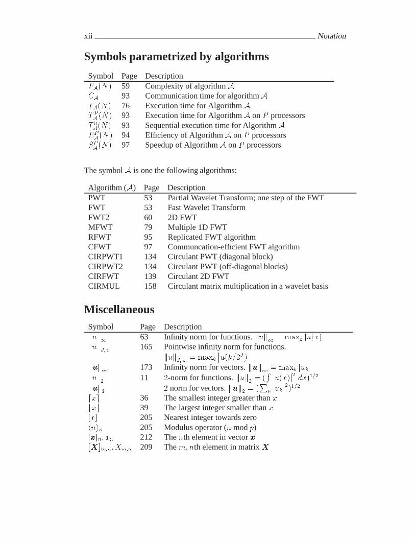
Symbols parametrized by algorithms
Symbol Page DescriptionFA�N� 59 Complexity of algorithm ACA 93 Communication time for algorithmATA�N� 76 Execution time for AlgorithmAT PA �N� 93 Execution time for AlgorithmA on P processors
T �A�N� 93 Sequential execution time for AlgorithmA
EPA�N� 94 Efficiency of AlgorithmA on P processors
SPA�N� 97 Speedup of AlgorithmA on P processors
The symbol A is one the following algorithms:
Algorithm (A) Page DescriptionPWT 53 Partial Wavelet Transform; one step of the FWTFWT 53 Fast Wavelet TransformFWT2 60 2D FWTMFWT 79 Multiple 1D FWTRFWT 95 Replicated FWT algorithmCFWT 97 Communcation-efficient FWT algorithmCIRPWT1 134 Circulant PWT (diagonal block)CIRPWT2 134 Circulant PWT (off-diagonal blocks)CIRFWT 139 Circulant 2D FWTCIRMUL 158 Circulant matrix multiplication in a wavelet basis
MiscellaneousSymbol Page Descriptionkuk� 63 Infinity norm for functions. kuk� � maxx ju�x�jkukJ�� 165 Pointwise infinity norm for functions.
kukJ�� � maxk��u�k��J ���
kuk� 173 Infinity norm for vectors. kuk� � maxk jukjkuk� 11 �-norm for functions. kuk� � �
R ju�x�j� dx����kuk� � norm for vectors. kuk� � �
Pk jukj�����
dxe 36 The smallest integer greater than xbxc 39 The largest integer smaller than xx� 205 Nearest integer towards zerohnip 205 Modulus operator (n mod p)x�n� xn 212 The nth element in vector xX�m�n�Xm�n 209 The m�nth element in matrix X

Contents
I Wavelets: Basic Theory and Algorithms 1
1 Motivation 31.1 Fourier expansion . . . . . . . . . . . . . . . . . . . . . . . . . . 31.2 Wavelet expansion . . . . . . . . . . . . . . . . . . . . . . . . . 6
2 Multiresolution analysis 112.1 Wavelets on the real line . . . . . . . . . . . . . . . . . . . . . . 112.2 Wavelets and the Fourier transform . . . . . . . . . . . . . . . . . 252.3 Periodized wavelets . . . . . . . . . . . . . . . . . . . . . . . . . 33
3 Wavelet algorithms 433.1 Numerical evaluation of � and � . . . . . . . . . . . . . . . . . . 433.2 Evaluation of scaling function expansions . . . . . . . . . . . . . 473.3 Fast Wavelet Transforms . . . . . . . . . . . . . . . . . . . . . . 52
4 Approximation properties 614.1 Accuracy of the multiresolution spaces . . . . . . . . . . . . . . . 614.2 Wavelet compression errors . . . . . . . . . . . . . . . . . . . . . 644.3 Scaling function coefficients or function values ? . . . . . . . . . 664.4 A compression example . . . . . . . . . . . . . . . . . . . . . . . 67
II Fast Wavelet Transforms on Supercomputers 71
5 Vectorization of the Fast Wavelet Transform 735.1 The Fujitsu VPP300 . . . . . . . . . . . . . . . . . . . . . . . . . 735.2 1D FWT . . . . . . . . . . . . . . . . . . . . . . . . . . . . . . . 745.3 Multiple 1D FWT . . . . . . . . . . . . . . . . . . . . . . . . . . 795.4 2D FWT . . . . . . . . . . . . . . . . . . . . . . . . . . . . . . . 815.5 Summary . . . . . . . . . . . . . . . . . . . . . . . . . . . . . . 84
xiii
xiv
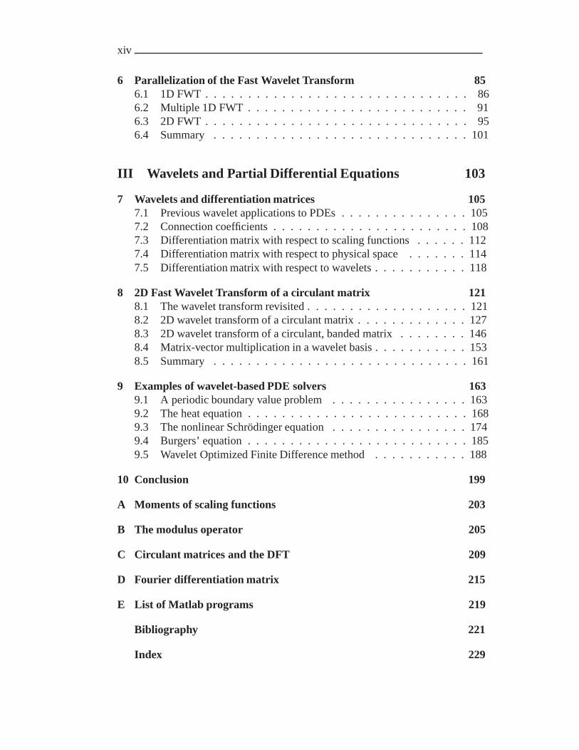
6 Parallelization of the Fast Wavelet Transform 856.1 1D FWT . . . . . . . . . . . . . . . . . . . . . . . . . . . . . . . 866.2 Multiple 1D FWT . . . . . . . . . . . . . . . . . . . . . . . . . . 916.3 2D FWT . . . . . . . . . . . . . . . . . . . . . . . . . . . . . . . 956.4 Summary . . . . . . . . . . . . . . . . . . . . . . . . . . . . . . 101
III Wavelets and Partial Differential Equations 103
7 Wavelets and differentiation matrices 1057.1 Previous wavelet applications to PDEs . . . . . . . . . . . . . . . 1057.2 Connection coefficients . . . . . . . . . . . . . . . . . . . . . . . 1087.3 Differentiation matrix with respect to scaling functions . . . . . . 1127.4 Differentiation matrix with respect to physical space . . . . . . . 1147.5 Differentiation matrix with respect to wavelets . . . . . . . . . . . 118
8 2D Fast Wavelet Transform of a circulant matrix 1218.1 The wavelet transform revisited . . . . . . . . . . . . . . . . . . . 1218.2 2D wavelet transform of a circulant matrix . . . . . . . . . . . . . 1278.3 2D wavelet transform of a circulant, banded matrix . . . . . . . . 1468.4 Matrix-vector multiplication in a wavelet basis . . . . . . . . . . . 1538.5 Summary . . . . . . . . . . . . . . . . . . . . . . . . . . . . . . 161
9 Examples of wavelet-based PDE solvers 1639.1 A periodic boundary value problem . . . . . . . . . . . . . . . . 1639.2 The heat equation . . . . . . . . . . . . . . . . . . . . . . . . . . 1689.3 The nonlinear Schrodinger equation . . . . . . . . . . . . . . . . 1749.4 Burgers’ equation . . . . . . . . . . . . . . . . . . . . . . . . . . 1859.5 Wavelet Optimized Finite Difference method . . . . . . . . . . . 188
10 Conclusion 199
A Moments of scaling functions 203
B The modulus operator 205
C Circulant matrices and the DFT 209
D Fourier differentiation matrix 215
E List of Matlab programs 219
Bibliography 221
Index 229

Part I
Wavelets: Basic Theory andAlgorithms


Chapter 1
Motivation
This section gives an introduction to wavelets accessible to non-specialists andserves at the same time as an introduction to key concepts and notation usedthroughout this study.
The wavelets considered in this introduction are called periodized Daubechieswavelets of genus four and they constitute a specific but representative exampleof wavelets in general. For the notation to be consistent with the rest of this work,we write our wavelets using the symbol ��j�l, the tilde signifying periodicity.
1.1 Fourier expansion
Many mathematical functions can be represented by a sum of fundamental orsimple functions denoted basis functions. Such representations are known as ex-pansions or series, a well-known example being the Fourier expansion
f�x� ��X
k���cke
i��kx� x � R (1.1)
which is valid for any reasonably well-behaved function f with period �. Here,the basis functions are complex exponentials ei��kx each representing a particularfrequency indexed by k. The Fourier expansion can be interpreted as follows: If fis a periodic signal, such as a musical tone, then (1.1) gives a decomposition of fas a superposition of harmonic modes with frequencies k (measured by cycles pertime unit). This is a good model for vibrations of a guitar string or an air columnin a wind instrument, hence the term “harmonic modes”.
The coefficients ck are given by the integral
ck �
Z �
�
f�x�e�i��kx dx

4 Motivation
0 1−0.5
0
0.5
x
Figure 1.1: The function f .
−512 −256 0 256 5120
0.1
Figure 1.2: Fourier coefficients of f .
Each coefficient ck can be conceived as the average harmonic content (over oneperiod) of f at frequency k. The coefficient c� is the average at frequency �, whichis just the ordinary average of f . In electrical engineering this term is known asthe “DC” term. The computation of ck is called the decomposition of f and theseries on the right hand side of (1.1) is called the reconstruction of f .
In theory, the reconstruction of f is exact, but in practice this is rarely so.Except in the occasional event where (1.1) can be evaluated analytically it mustbe truncated in order to be computed numerically. Furthermore, one often wantsto save computational resources by discarding many of the smallest coefficientsck. These measures naturally introduce an approximation error.
To illustrate, consider the sawtooth function
f�x� �
�x � � x � ���x� � ��� � x � �

1.1 Fourier expansion 5
0 1−0.6
0
0.6
x
Figure 1.3: A function f and a truncated Fourier expansion with only 17 terms
which is shown in Figure 1.1. The Fourier coefficients ck of the truncated expan-sion
N��Xk��N����
ckei��kx
are shown in Figure 1.2 for N � ����.
If, for example, we retain only the �� largest coefficients, we obtain the trun-cated expansion shown in Figure 1.3. While this approximation reflects some ofthe behavior of f , it does not do a good job for the discontinuity at x � ���. It isan interesting and well-known fact that such a discontinuity is perfectly resolvedby the series in (1.1), even though the individual terms themselves are continuous.However, with only a finite number of terms this will not be the case. In addi-tion, and this is very unfortunate, the approximation error is not restricted to thediscontinuity but spills into much of the surrounding area. This is known as theGibbs phenomenon.
The underlying reason for the poor approximation of the discontinuous func-tion lies in the nature of complex exponentials, as they all cover the entire intervaland differ only with respect to frequency. While such functions are fine for rep-resenting the behavior of a guitar string, they are not suitable for a discontinuousfunction. Since each of the Fourier coefficient reflects the average content of acertain frequency, it is impossible to see where a singularity is located by lookingonly at individual coefficients. The information about position can be recoveredonly by computing all of them.

6 Motivation
1.2 Wavelet expansion
The problem mentioned above is one way of motivating the use of wavelets. Likethe complex exponentials, wavelets can be used as basis functions for the expan-sion of a function f . Unlike the complex exponentials, they are able to capturethe positional information about f as well as information about scale. The lat-ter is essentially equivalent to frequency information. A wavelet expansion for a�-periodic function f has the form
f�x� �
�J���Xk��
cJ��k��J��k�x� �
�Xj�J�
�j��Xk��
dj�k ��j�k�x�� x � R (1.2)
where J� is a non-negative integer. This expansion is similar to the Fourier expan-sion (1.1): It is a linear combination of a set of basis functions, and the waveletcoefficients are given by
cJ��k �
Z �
�
f�x���J��k�x� dx
dj�k �
Z �
�
f�x� ��j�k�x� dx
One immediate difference with respect to the Fourier expansion is the fact thatnow we have two types of basis functions and that both are indexed by two inte-gers. The ��J��k are called scaling functions and the ��j�k are called wavelets. Bothhave compact support such that
��j�k�x� � ��j�k�x� � � for x ���k
�j�k � �
�j
�We call j the scale parameter because it scales the width of the support, and k theshift parameter because it translates the support interval. There are generally noexplicit formulas for ��j�k and ��j�k but their function values are computable and soare the above coefficients. The scaling function coefficient cJ��k can be interpretedas a local weighted average of f in the region where ��J� �k is non-zero. On theother hand, the wavelet coefficients dj�k represent the opposite property, namelythe details of f that are lost in the weighted average.
In practice, the wavelet expansion (like the Fourier expansion) must be trun-cated at some finest scale which we denote J��: The truncated wavelet expansionis
�J���Xk��
cJ��k��J��k�x� �
J��Xj�J�
�j��Xk��
dj�k ��j�k�x�

1.2 Wavelet expansion 7
0 64 128 256 512 1024−6
−4
−2
0
2
4
6
Figure 1.4: Wavelet coefficients of f .
and the wavelet coefficients ordered as
nfcJ��kg�
J���k�� � ffdj�kg�j��k�� gJ��j�J�
o
are shown in Figure 1.4. The wavelet expansion (1.2) can be understood as fol-lows: The first sum is a coarse representation of f , where f has been replacedby a linear combination of �J� translations of the scaling function ��J���. This cor-responds to a Fourier expansion where only low frequencies are retained. Theremaining terms are refinements. For each j a layer represented by �j translationsof the wavelet ��j�� is added to obtain a successively more detailed approximationof f . It is convenient to define the approximation spaces
�Vj � spanf��j�kg�j��
k��
�Wj � spanf ��j�kg�j��
k��
These spaces are related such that
�VJ � �VJ� � �WJ� � � � � � �WJ��
The coarse approximation of f belongs to the space �VJ� and the successive re-finements are in the spaces �Wj for j � J�� J� � �� � � � � J � �. Together, all ofthese contributions constitute a refined approximation of f . Figure 1.5 shows thescaling functions and wavelets corresponding to �V�� �W� and �W�.

8 Motivation
Scaling functions in �V�: ����k�x�� k � �� � � �
Wavelets in �W�: ����k�x�� k � �� � � �
Wavelets in �W�: ���k�x�� k � �� � � � � � �
Figure 1.5: There are four scaling functions in �V� and four wavelets in �W� but eightmore localized wavelets in �W�.

1.2 Wavelet expansion 9
0 1
V6
W6
W7
W8
W9
V10
~
~
~
~
~
~
Figure 1.6: The top graph is the sum of its projections onto a coarse space �V and asequence of finer spaces �W – �W�.
Figure 1.6 shows the wavelet decomposition of f organized according to scale:Each graph is a projection of f onto one of the approximation spaces mentionedabove. The bottom graph is the coarse approximation of f in �V . Those labeled�W to �W� are successive refinements. Adding these projections yields the graph
labeled �V��.Figure 1.4 and Figure 1.6 suggest that many of the wavelet coefficients are
zero. However, at all scales there are some non-zero coefficients, and they revealthe position where f is discontinuous. If, as in the Fourier case, we retain only the�� largest wavelet coefficients, we obtain the approximation shown in Figure 1.7.Because of the way wavelets work, the approximation error is much smaller thanthat of the truncated Fourier expansion and, very significantly, is highly localizedat the point of discontinuity.

10 Motivation
0 1−0.6
0
0.6
x
Figure 1.7: A function f and a truncated wavelet expansion with only 17 terms
1.2.1 Summary
There are three important facts to note about the wavelet approximation:
1. The good resolution of the discontinuity is a consequence of the large waveletcoefficients appearing at the fine scales. The local high frequency content atthe discontinuity is captured much better than with the Fourier expansion.
2. The fact that the error is restricted to a small neighborhood of the discon-tinuity is a result of the “locality” of wavelets. The behavior of f at onelocation affects only the coefficients of wavelets close to that location.
3. Most of the linear part of f is represented exactly. In Figure 1.6 one can seethat the linear part of f is approximated exactly even in the coarsest approx-imation space �V where only a few scaling functions are used. Therefore,no wavelets are needed to add further details to these parts of f .
The observation made in � is a manifestation of a property called vanishing mo-ments which means that the scaling functions can locally represent low order poly-nomials exactly. This property is crucial to the success of wavelet approximationsand it is described in detail in Sections 2.1.5 and 2.1.6.
The Matlab function wavecompare conducts this comparison experiment andthe function basisdemo generates the basis functions shown in Figure 1.5.

Chapter 2
Multiresolution analysis
2.1 Wavelets on the real line
A natural framework for wavelet theory is multiresolution analysis (MRA) whichis a mathematical construction that characterizes wavelets in a general way. MRAyields fundamental insights into wavelet theory and leads to important algorithmsas well. The goal of MRA is to express an arbitrary function f � L��R� at variouslevels of detail. MRA is characterized by the following axioms:
f�g � � � V�� V� V� � � � L��R� �a�
��j���
Vj � L��R� �b�
f��x� k�gk�Z is an orthonormal basis for V� �c�
f � Vj f���� � Vj�� �d�
(2.1)
This describes a sequence of nested approximation spaces Vj in L��R� suchthat the closure of their union equals L��R�. Projections of a function f � L��R�onto Vj are approximations to f which converge to f as j ��. Furthermore, thespace V� has an orthonormal basis consisting of integral translations of a certainfunction �. Finally, the spaces are related by the requirement that a function fmoves from Vj to Vj�� when rescaled by �. From (2.1c) we have the normalization(in the L�-norm)
k�k� Z �
��j��x�j� dx
���
� �
12 Multiresolution analysis
and it is also required that � has unit area [JS94, p. 383], [Dau92, p. 175], i.e.Z �
����x� dx � � (2.2)
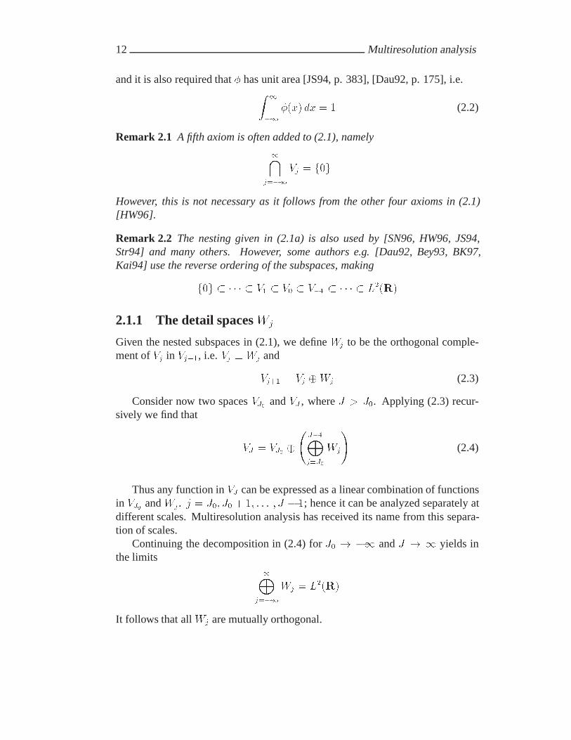
Remark 2.1 A fifth axiom is often added to (2.1), namely
��j���
Vj � f�g
However, this is not necessary as it follows from the other four axioms in (2.1)[HW96].
Remark 2.2 The nesting given in (2.1a) is also used by [SN96, HW96, JS94,Str94] and many others. However, some authors e.g. [Dau92, Bey93, BK97,Kai94] use the reverse ordering of the subspaces, making
f�g � � � V� V� V�� � � � L��R�
2.1.1 The detail spaces Wj
Given the nested subspaces in (2.1), we define Wj to be the orthogonal comple-ment of Vj in Vj��, i.e. Vj �Wj and
Vj�� � Vj �Wj (2.3)
Consider now two spaces VJ� and VJ , where J � J�. Applying (2.3) recur-sively we find that
VJ � VJ� ��
J��Mj�J�
Wj
(2.4)
Thus any function in VJ can be expressed as a linear combination of functionsin VJ� and Wj� j � J�� J� � �� � � � � J � �; hence it can be analyzed separately atdifferent scales. Multiresolution analysis has received its name from this separa-tion of scales.
Continuing the decomposition in (2.4) for J� � �� and J � � yields inthe limits
�Mj���
Wj � L��R�
It follows that all Wj are mutually orthogonal.

2.1 Wavelets on the real line 13
Remark 2.3 Wj can be chosen such that it is not orthogonal to Vj . In that caseMRA will lead to the so-called bi-orthogonal wavelets [JS94]. We will not addressthis point further but only mention that bi-orthogonal wavelets are more flexiblethan orthogonal wavelets. We refer to [SN96] or [Dau92] for details.
2.1.2 Basic scaling function and basic wavelet
Since the set f��x � k�gk�Z is an orthonormal basis for V� by axiom (2.1c) itfollows by repeated application of axiom ����d� that
f���jx� k�gk�Z (2.5)
is an orthogonal basis for Vj . Note that (2.5) is the function ���jx� translated byk��j , i.e. it becomes narrower and translations get smaller as j grows. Since thesquared norm of one of these basis functions isZ �
��
�����jx� k���� dx � ��j
Z �
��j��y�j� dy � ��j k�k�� � ��j
it follows that
f�j�����jx� k�gk�Z is an orthonormal basis for Vj
Similarly, it is shown in [Dau92, p. 135] that there exists a function ��x� suchthat
f�j�����jx� k�gk�Z is an orthonormal basis for Wj
We call � the basic scaling function and � the basic wavelet1. It is generally notpossible to express either of them explicitly, but, as we shall see, there are efficientand elegant ways of working with them, regardless. It is convenient to introducethe notations
�j�k�x� � �j�����jx� k�
�j�k�x� � �j�����jx� k�(2.6)
and
�k�x� � ���k�x�
�k�x� � ���k�x�(2.7)
1In the literature � is often referred to as the mother wavelet.

14 Multiresolution analysis
We will use the long and short forms interchangeably depending on the givencontext.
Since �j�k � Wj it follows immediately that �j�k is orthogonal to �j�k because�j�k � Vj and Vj � Wj . Also, because all Wj are mutually orthogonal, it followsthat the wavelets are orthogonal across scales. Therefore, we have the orthogonal-ity relations Z �
���j�k�x��j�l�x� dx � k�l (2.8)Z �
���i�k�x��j�l�x� dx � i�jk�l (2.9)Z �
���i�k�x��j�l�x� dx � �� j � i (2.10)
where i� j� k� l � Z and k�l is the Kronecker delta defined as
k�l �
�� k �� l� k � l
2.1.3 Expansions of a function in VJ
A function f � VJ can be expanded in various ways. For example, there is thepure scaling function expansion
f�x� ��X
l���cJ�l�J�l�x�� x � R (2.11)
where
cJ�l �
Z �
��f�x��J�l�x� dx (2.12)
For any J� � J there is also the wavelet expansion
f�x� ��X
l���cJ��l�J��l�x� �
J��Xj�J�
�Xl���
dj�l�j�l�x�� x � R (2.13)
where
cJ��l �
Z �
��f�x��J��l�x� dx
dj�l �
Z �
��f�x��j�l�x� dx (2.14)

2.1 Wavelets on the real line 15
Note that the choice J� � J in (2.13) yields (2.11) as a special case. We define
� � J � J� (2.15)
and denote � the depth of the wavelet expansion. From the orthonormality ofscaling functions and wavelets we find that
kfk�� ��X
k���jcJ�kj� �
�Xk���
jcJ��kj� �J��Xj�J�
�Xk���
jdj�kj�
which is Parseval’s equation for wavelets.
Definition 2.1 Let PVj and PWj denote the operators that project any f � L��R�orthogonally onto Vj and Wj , respectively. Then
�PVjf��x� �
�Xl���
cj�l�j�l�x�
�PWjf��x� ��X
l���dj�l�j�l�x�
where
cj�l �
Z �
��f�x��j�l�x� dx
dj�l �
Z �
��f�x��j�l�x� dx
and
PVJf � PVJ�f �
J��Xj�J�
PWjf
2.1.4 Dilation equation and wavelet equation
Since V� V�, any function in V� can be expanded in terms of basis functions ofV�. In particular, ��x� � �����x� � V� so
��x� ��X
k���ak���k�x� �
p�
�Xk���
ak���x� k�
16 Multiresolution analysis
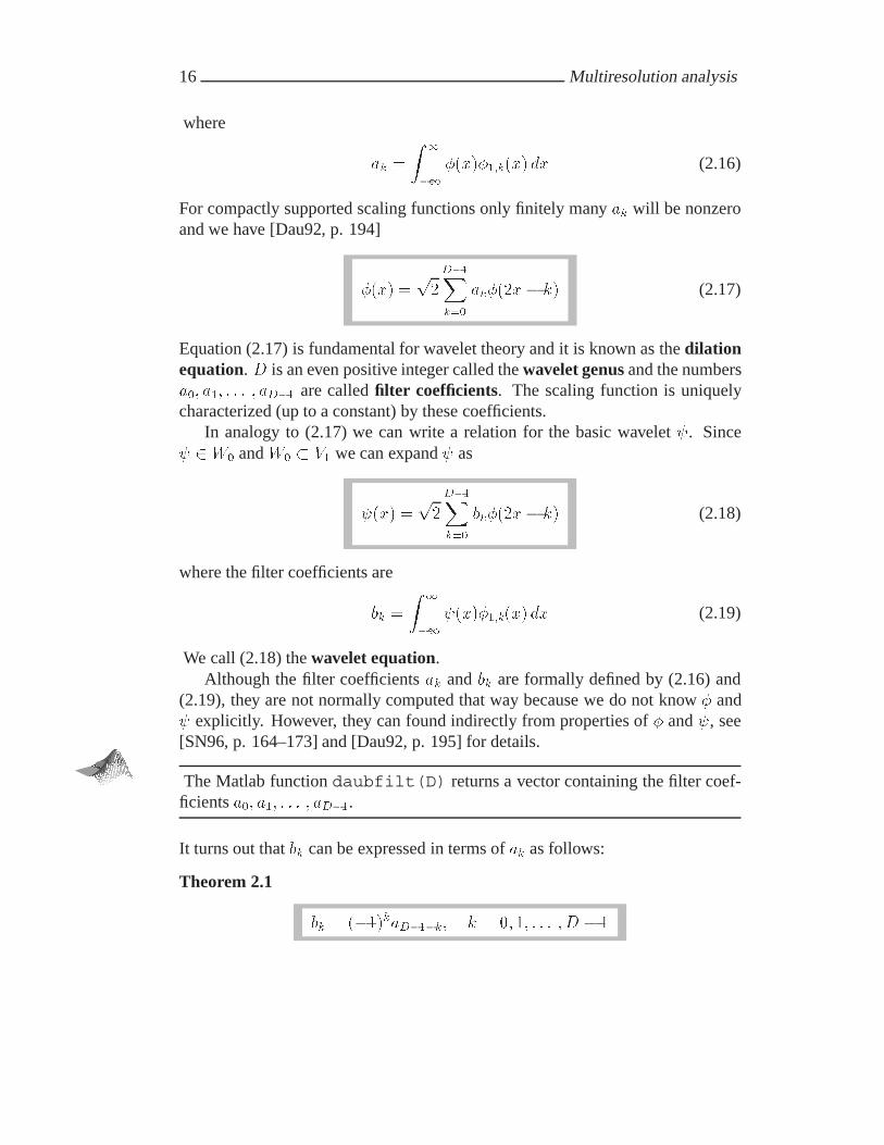
where
ak �
Z �
����x����k�x� dx (2.16)
For compactly supported scaling functions only finitely many ak will be nonzeroand we have [Dau92, p. 194]
��x� �p�D��Xk��
ak���x� k� (2.17)
Equation (2.17) is fundamental for wavelet theory and it is known as the dilationequation. D is an even positive integer called the wavelet genus and the numbersa�� a�� � � � � aD�� are called filter coefficients. The scaling function is uniquelycharacterized (up to a constant) by these coefficients.
In analogy to (2.17) we can write a relation for the basic wavelet �. Since� � W� and W� V� we can expand � as
��x� �p�
D��Xk��
bk���x� k� (2.18)
where the filter coefficients are
bk �
Z �
����x����k�x� dx (2.19)
We call (2.18) the wavelet equation.Although the filter coefficients ak and bk are formally defined by (2.16) and
(2.19), they are not normally computed that way because we do not know � and� explicitly. However, they can found indirectly from properties of � and �, see[SN96, p. 164–173] and [Dau92, p. 195] for details.
The Matlab function daubfilt(D) returns a vector containing the filter coef-ficients a�� a�� � � � � aD��.
It turns out that bk can be expressed in terms of ak as follows:
Theorem 2.1
bk � ����kaD���k� k � �� �� � � � �D � �

2.1 Wavelets on the real line 17
Proof: It follows from (2.10) thatR��� ��x���x� dx � �. Using (2.17) and (2.18)
we then haveZ �
����x���x� dx � �
Z �
��
D��Xk��
ak���x� k�
D��Xl��
bl���x� l� dx
�D��Xk��
D��Xl��
akbl
Z �
����y � k���y � l� dy� �z �
� k�l
�
D��Xk��
akbk � �
This relation is fulfilled if either ak � � or bk � � for all k, the trivial solutions,or if bk � ����kam�k where m is an odd integer provided that we set am�k � �form� k �� ��D� ��. In the latter case the terms apbp will cancel with the termsam�pbm�p for p � �� �� � � � � �m� ���� � �. An obvious choice is m � D � �. �
The Matlab function low2hi computes fbkgD��k�� from fakgD��k�� .
One important consequence of (2.17) and (2.18) is that supp��� � supp��� ���D � �� (see e.g. [Dau92, p. 176] or [SN96, p. 185]). It follows immediatelythat
supp��j�l� � supp��j�l� � Ij�l (2.20)
where
Ij�l �
�l
�j�l�D � �
�j
�(2.21)
Remark 2.4 The formulation of the dilation equation is not the same throughoutthe literature. We have identified three versions:
1. ��x� �P
k ak���x� k�
2. ��x� �p�P
k ak���x� k�
3. ��x� � �P
k ak���x� k�
18 Multiresolution analysis
The first is used by e.g. [WA94, Str94], the second by e.g. [Dau92, Bey93,Kai94], and the third by e.g. [HW96, JS94]. We have chosen the second formu-lation, partly because it comes directly from the MRA expansion of � in terms of���k but also because it leads to orthonormality of the wavelet transform matrices,see Section 3.3.2.
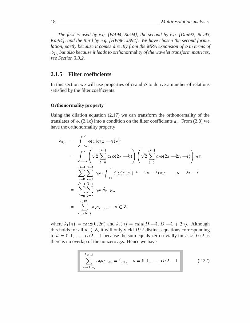
2.1.5 Filter coefficients
In this section we will use properties of � and � to derive a number of relationssatisfied by the filter coefficients.
Orthonormality property
Using the dilation equation (2.17) we can transform the orthonormality of thetranslates of �, (2.1c) into a condition on the filter coefficients ak. From (2.8) wehave the orthonormality property
��n �
Z �
����x���x� n� dx
�
Z �
��
�p�D��Xk��
ak���x� k�
�p�D��Xl��
al���x� �n� l�
dx
�D��Xk��
D��Xl��
akal
Z �
����y���y � k � �n � l� dy� y � �x� k
�
D��Xk��
D��Xl��
akalk��n�l
�
k��n�Xk�k��n�
akak��n� n � Z
where k��n� � max��� �n� and k��n� � min�D � ��D � � � �n�. Althoughthis holds for all n � Z, it will only yield D�� distinct equations correspondingto n � �� �� � � � �D�� � � because the sum equals zero trivially for n � D�� asthere is no overlap of the nonzero aks. Hence we have
k��n�Xk�k��n�
akak��n � ��n� n � �� �� � � � �D�� � � (2.22)

2.1 Wavelets on the real line 19
Similarly, it follows from Theorem 2.1 that
k��n�Xk�k��n�
bkbk��n � ��n� n � �� �� � � � �D�� � � (2.23)
Conservation of area
Recall thatR��� ��x� dx � �. Integration of both sides of (2.17) then gives
Z �
����x� dx �
p�D��Xk��
ak
Z �
�����x� k� dx �
�p�
D��Xk��
ak
Z �
����y� dy
or
D��Xk��
ak �p� (2.24)
The name “conservation of area” is suggested by Newland [New93, p. 308].
Property of vanishing moments
Another important property of the scaling function is its ability to represent poly-nomials exactly up to some degree P � �. More precisely, it is required that
xp ��X
k���Mp
k��x� k�� x � R� p � �� �� � � � � P � � (2.25)
where
Mpk �
Z �
��xp��x� k� dx� k � Z� p � �� �� � � � � P � � (2.26)
We denoteMpk the pth moment of ��x�k� and it can be computed by a procedure
which is described in Appendix A.Equation (2.25) can be translated into a condition involving the wavelet by
taking the inner product with ��x�. This yieldsZ �
��xp��x� dx �
�Xk���
Mpk
Z �
����x� k���x� dx � �

20 Multiresolution analysis
since � and � are orthonormal. Hence, we have the property of P vanishingmoments: Z �
��xp��x� dx � �� x � R� p � �� �� � � � � P � � (2.27)
The property of vanishing moments can be expressed in terms of the filtercoefficients as follows. Substituting the wavelet equation (2.18) into (2.27) yields
� �
Z �
��xp��x� dx
�p�D��Xk��
bk
Z �
��xp���x� k� dx
�
p�
�p��
D��Xk��
bk
Z �
���y � k�p��y� dy� y � �x� k
�
p�
�p��
D��Xk��
bk
pXn��
p
n
kn
Z �
��yp�n��y� dy
�
p�
�p��
pXn��
p
n
Mp�n
�
D��Xk��
bkkn (2.28)
where we have used (2.26) and the binomial formula
�y � k�p �
pXn��
p
n
yp�nkn
For p � � relation (2.28) becomesPD��
k�� bk � �, and using induction on p weobtain P moment conditions on the filter coefficients, namely
D��Xk��
bkkp �
D��Xk��
����kaD���kkp � �� p � �� �� � � � � P � �
This expression can be simplified further by the change of variables l � D���k.Then
� �D��Xl��
����D���lal�D � � � l�p
and using the binomial formula again, we arrive at
D��Xl��
����lallp � �� p � �� �� � � � � P � � (2.29)

2.1 Wavelets on the real line 21
Other properties
The conditions (2.22), (2.24) and (2.29) comprise a system of D�� ���P equa-tions for the D filter coefficients ak� k � �� �� � � � �D � �. However, it turns outthat one of the conditions is redundant. For example (2.29) with p � � can beobtained from the others, see [New93, p. 320]. This leaves a total of D�� � Pequations for the D filter coefficients. Not surprisingly, it can be shown [Dau92,p. 194] that the highest number of vanishing moments for this type of wavelet is
P � D��
yielding a total of D equations that must be fulfilled.This system can be used to determine filter coefficients for compactly sup-
ported wavelets or used to validate coefficients obtained otherwise.
The Matlab function filttest checks if a vector of filter coefficients fulfils(2.22), (2.24) and (2.29) with P � D��.
Finally we note two other properties of the filter coefficients.
Theorem 2.2
D����Xk��
a�k �
D����Xk��
a�k�� ��p�
Proof: Adding (2.24) and (2.29) with p � � yields the first result. Subtractingthem yields the second. �
Theorem 2.3
D����Xl��
D��l��Xn��
anan��l�� ��
�
Proof: Using (2.29) twice we write
� �
�D��Xk��
����kak �
D��Xl��
�����lal
�D��Xk��
D��Xl��
����k�lakal
�
D��Xk��
a�k� �z ���
�
D��Xk��
k��Xl��
����k�lakal �D��Xk��
D��Xl�k��
����l�kakal

22 Multiresolution analysis
Using (2.22) with n � � in the first sum and rearranging the other sums yields
� � � �
D��Xp��
D���pXl��
����pal�pal �D��Xp��
D���pXk��
����pakak�p
� � � �D��Xp��
D���pXn��
����panan�p
All sums where p is even vanish by (2.22), so we are left with the “odd” terms(p � �l � �)
� � � � �
D����Xl��
�����l��D��l��Xn��
anan��l��
� � � �
D����Xl��
D��l��Xn��
anan��l��
from which the result follows. �
Equation (2.24) can now be derived directly from (2.22) and (2.29) and havethe following Corollary of Theorem 2.2.
Corollary 2.4
D��Xk��
�p�
Proof: By a manipulation similar to that of Theorem 2.2 we write�D��Xk��
ak
�D��Xl��
al
�
D��Xk��
D��Xl��
akal
� � � �
D����Xl��
D��l��Xn��
anan��l��
� �
where Theorem 2.2 was used for the last equation. Taking the square root on eachside yields the result. �

2.1 Wavelets on the real line 23
2.1.6 Decay of wavelet coefficients
The P vanishing moments have an important consequence for the wavelet coef-ficients dj�k (2.14): They decrease rapidly for a smooth function. Furthermore,if a function has a discontinuity in one of its derivatives then the wavelet coeffi-cients will decrease slowly only close to that discontinuity and maintain fast decaywhere the function is smooth. This property makes wavelets particularly suitablefor representing piecewise smooth functions. The decay of wavelet coefficients isexpressed in the following theorem:
Theorem 2.5 Let P � D�� be the number of vanishing moments for a wavelet�j�k and let f � CP �R�. Then the wavelet coefficients given in (2.14) decay asfollows:
jdj�kj � CP ��j�P��� � max
��Ij�k
��f �P ������where CP is a constant independent of j, k, and f and Ij�k � suppf�j�kg �k��j� �k �D � ����j �.
Proof: For x � Ij�k we write the Taylor expansion for f around x � k��j .
f�x� �
�P��Xp��
f �p��k��j
� �x� k�j�p
p�
� f �P ����
�x� k�j�P
P �(2.30)
where � � k��j � x�.Inserting (2.30) into (2.14) and restricting the integral to the support of �j�k
yields
dj�k �
ZIj�k
f�x��j�k�x� dx
�
�P��Xp��
f �p��k��j
� �
p�
ZIj�k
x� k
�j
p
�j�k�x� dx
�
�
P �
ZIj�k
f �P ����
x� k
�j
P
�j�k�x� dx
Recall that � depends on x, so f�P ���� is not constant and must remain under thelast integral sign.

24 Multiresolution analysis
Consider the integrals where p � �� �� � � � � P � �. Using (2.21) and lettingy � �jx� k we obtain
Z �k�D�����j
k��j
x� k
�j
p
�j�����jx� k� dx
� �j��Z D��
�
� y
�j
�p��y� ��jdy
� ��j�p�����Z D��
�
yp��y� dy
� �� p � �� �� � � � � P � �
because of the P vanishing moments (2.27). Therefore, the wavelet coefficient isdetermined from the remainder term alone. Hence,
jdj�kj ��
P �
�����ZIj�k
f �P ����
x� k
�j
P
�j�����jx� k� dx
������ �
P �max��Ij�k
��f �P ������ ZIj�k
�����x� k
�j
P
�j�����jx� k�
����� dx� ��j�P�����
�
P �max��Ij�k
��f �P ������ Z D��
�
��yP��y��� dyDefining
CP ��
P �
Z D��
�
��yP��y��� dywe obtain the desired inequality. �
From Theorem 2.5 we see that if f behaves like a polynomial of degree less thanP in the interval Ij�k then f �P � � and the corresponding wavelet coefficientdj�k is zero. If f �P � is different from zero, coefficients will decay exponentiallywith respect to the scale parameter j. If f has a discontinuity in a derivativeof order less than or equal to P , then Theorem 2.5 does not hold for waveletcoefficients located at the discontinuity2. However, coefficients away from thediscontinuity are not affected. The coefficients in a wavelet expansion thus reflectlocal properties of f and isolated discontinuities do not ruin the convergence awayfrom the discontinuities. This means that functions that are piecewise smooth havemany small wavelet coefficients in their expansions and may thus be represented
2There are D � � affected wavelet coefficients at each level

2.2 Wavelets and the Fourier transform 25
well by relatively few wavelet coefficients. This is the principle behind waveletbased data compression and one of the reasons why wavelets are so useful ine.g. signal processing applications. We saw an example of this in Chapter 1 andSection 4.4 gives another example. The consequences of Theorem 2.5 with respectto approximation errors of wavelet expansions are treated in Chapter 4.
2.2 Wavelets and the Fourier transform
It is often useful to consider the behavior of the Fourier transform of a functionrather than the function itself. Also in case it gives rise to some intriguing relationsand insights about the basic scaling function and the basic wavelet.We define the (continuous) Fourier transform as
���� �
Z �
����x�e�i�x dx� � � R
The requirement that � has unit area (2.2) immediately translates into
���� �
Z �
����x� dx � � (2.31)
Our point of departure for expressing � at other values of � is the dilation equation(2.17). Taking the Fourier transform on both sides yields
���� �p�D��Xk��
ak
Z �
�����x� k�e�i�x dx
�p�
D��Xk��
ak
Z �
����y�e�i��y�k��� dy��
��p�
D��Xk��
ake�ik���
Z �
����y�e�i�����y dy
� A
�
�
�
�
�
(2.32)
where
A��� ��p�
D��Xk��
ake�ik�� � � R (2.33)
A��� is a ��-periodic function with some interesting properties which can bederived directly from the conditions on the filter coefficients established in Sec-tion 2.1.

26 Multiresolution analysis
Lemma 2.6 If � has P vanishing moments then
A��� � �dp
d�pA��� j��� � �� p � �� �� � � � � P � �
Proof: Let � � � in (2.33). Using (2.24) we find immediately
A��� ��p�
D��Xk��
ak �
p�p�� �
Now let � � �. Then by (2.29)
dp
d�pA��� j��� �
�p�
D��Xk��
��ik�pake�ik�
��p���i�p
D��Xk��
kpak����k
� �� p � �� �� � � � � P � �
�
Putting p � � in Lemma 2.6 and using the �� periodicity of A��� we obtain
Corollary 2.7
A�n�� �
�� n even� n odd
Equation (2.32) can be repeated for ������ yielding
���� � A
�
�
A
�
�
�
�
�
After N such steps we have
���� �NYj��
A
�
�j
�
�
�N

2.2 Wavelets and the Fourier transform 27
It follows from (2.33) and (2.24) that jA���j � � so the product converges forN �� and we get the expression
���� ��Yj��
A
�
�j
� ���
Using (2.31) we arrive at the product formula
���� ��Yj��
A
�
�j
� � � R (2.34)
Lemma 2.8
����n� � ��n� n � Z
Proof: The case n � � follows from (2.31). Therefore, let n � Z n f�g beexpressed in the form n � �iK where i � N� and K � Z with K odd, i.e.hKi� � �. Then using (2.34) we get
����n� ��Yj��
A
��n
�j
�
�Yj��
A
�i��K�
�j
� A��iK��A��i��K�� � � �A�K�� � � �
� �
since A�K�� � � by Corollary 2.7. �
A consequence of Lemma 2.8 is the following basic property of �:
Theorem 2.9
�Xn���
�j���x� n� � ��j��� j � �� x � R

28 Multiresolution analysis
Proof: Let
Sj�x� ��X
n����j���x� n�
We observe that Sj�x� is a �-periodic function. Hence it has the Fourier seriesexpansion
Sj�x� ��X
k���cke
i��kx� x � R (2.35)
where the Fourier coefficients ck are defined by
ck �
Z �
�
Sj�x�e�i��kx dx
�
Z �
�
�Xn���
�j���x� n�e�i��kx dx
��X
n���
Z n��
n
�j���y�e�i��ky ei��kn� �z �
��
dy� y � x� n
�
Z �
���j���y�e
�i��ky dy
� �j��Z �
�����jy�e�i��ky dy
� �j��Z �
����z�e�i��k�
�jz ��jdz� z � �jy
� ��j�� ����k��j�� k � Z
We know from Lemma 2.8 that ����k� � ��k. Therefore, since j � � by as-sumption,
ck � ��j�� ����k��j� � ��j����k
so the Fourier series collapses into one term, namely the “DC” term c�, i.e.
Sj�x� � c� � ��j��
from which the result follows. �

2.2 Wavelets and the Fourier transform 29
Theorem 2.9 states that if � is a zero of the function A��� then the constantfunction can be represented by a linear combination of the translates of �j���x�,which again is equivalent to the zeroth vanishing moment condition (2.27). If thenumber of vanishing moments P is greater than one, then a similar argument canbe used to show the following more general statement [SN96, p. 230]
Theorem 2.10 If � is a zero of A��� of multiplicity P , i.e. if
dp
d�pA��� j��� � �� p � �� �� � � � � P � �
then:
1. The integral translates of ��x� can reproduce polynomials of degree lessthan P .
2. The wavelet ��x� has P vanishing moments.
3. ��p����n� � � for n � Z, n �� � and p � P .
4. ��p���� � � for p � P .
2.2.1 The wavelet equation
In the beginning of this section we obtained a relation (2.32) for the scaling func-tion in the frequency domain. Using (2.18) we can obtain an analogous expressionfor �.
���� �p�
D��Xk��
bk
Z �
�����x� k�e�i�x dx
��p�
D��Xk��
bke�ik���
Z �
����y�e�i�����y dy
� B
�
�
�
�
�
where
B��� ��p�
D��Xk��
bke�ik� (2.36)

30 Multiresolution analysis
Using Theorem 2.1 we can express B��� in terms of A���.
B��� ��p�
D��Xk��
����kaD���ke�ik�
��p�
D��Xk��
aD���ke�ik�����
��p�
D��Xl��
ale�i�D���l������
� e�i�D���������p�
D��Xl��
aleil�����
� e�i�D��������A�� � ��
This leads to the wavelet equation in the frequency domain.
���� � e�i�D����������A ���� � ��� ����� (2.37)
An immediate consequence of (2.37) is the following lemma:
Lemma 2.11
����n� � �� n � Z
Proof: Letting � � ��n in (2.37) yields
����n� � e�i�D������n���A ���n� ��� ���n�
which is equal to zero by Lemma 2.8 for n �� �. For n � � we have
���� � �A ���
but this is also zero by Corollary 2.7. �
2.2.2 Orthonormality in the frequency domain
The inner products of � with its integral translates also have an interesting formu-lation in the frequency domain. By Plancherel’s identity [HW96, p. 4] the inner

2.2 Wavelets and the Fourier transform 31
product in the physical domain equals the inner product in the frequency domain(except for a factor of ��). Hence
fk �
Z �
����x���x� k� dx
��
��
Z �
����������e�i�k d�
��
��
Z �
��
����������� ei�k d��
�
��
Z ��
�
�Xn���
������ � ��n����� ei�k d� (2.38)
Define
F ��� ��X
n���
������ � ��n����� � � � R (2.39)
Then we see from (2.38) that fk is the k’th Fourier coefficient of F ���. Thus
F ��� �
�Xk���
fke�ik� (2.40)
Since � is orthogonal to its integral translations we know from (2.8) that
fk �
�� k � �� k �� �
hence (2.40) evaluates to
F ��� � �� � � R
Thus we have proved the following lemma.
Lemma 2.12 The translates ��x� k�, k � Z are orthonormal if and only if
F ��� �

32 Multiresolution analysis
We can now translate the condition on F into a condition on A���. From (2.32)and (2.39) we have
F ���� ��X
n���
������� � ��n�����
��X
n���
������ � �n����� jA�� � �n�j�
Splitting the sum into two sums according to whether n is even or odd and usingthe periodicity of A��� yields
F ���� �
�Xn���
������ � ��n����� jA�� � ��n�j� �
�Xn���
������ � � � ��n����� jA�� � � � ��n�j�
� jA���j��X
n���
������ � ��n����� � jA�� � ��j�
�Xn���
������ � � � ��n�����
� jA���j� F ��� � jA�� � ��j� F �� � ��
If F ��� � � then jA���j� � jA�� � ��j� � and the converse is also true [SN96,p. 205–206], [JS94, p. 386]. For this reason we have
Lemma 2.13
F ��� � jA���j� � jA�� � ��j� �
Finally, Lemma 2.12 and Lemma 2.13 yields the following theorem:
Theorem 2.14 The translates ��x� k�, k � Z are orthonormal if and only if
jA���j� � jA�� � ��j� �
2.2.3 Overview of conditions
We summarize now various formulations of the orthonormality property, the prop-erty of vanishing moments and the conservation of area.

2.3 Periodized wavelets 33
Orthonormality property:
Z �
����x���x� k� dx � ��k� k � ZD��Xk��
akak��n � ��n� n � Z
jA���j� � jA�� � ��j� �� � � R
Property of vanishing moments:
For p � �� �� � � � � P � � and P � D�� we haveZ �
����x�xp dx � �
D��Xk��
����kakkp � �
dp
d�pA��� j���� �
Conservation of area:
��x� �p�D��Xk��
ak���x� k�� x � R
D��Xk��
ak �p�
A��� � �
2.3 Periodized wavelets
So far our functions have been defined on the entire real line, e.g. f � L��R�.There are applications, such as the processing of audio signals, where this is areasonable model because audio signals can be arbitrarily long and the total lengthmay be unknown until the moment when the audio signal stops. However, in mostpractical applications such as image processing, data fitting, or problems involvingdifferential equations, the space domain is a finite interval. Many of these casescan be dealt with by introducing periodized scaling functions and wavelets whichwe define as follows:

34 Multiresolution analysis
Definition 2.2 Let � � L��R� and � � L��R� be the basic scaling function andthe basic wavelet from a multiresolution analysis as defined in (2.1). For anyj� l � Z we define the �-periodic scaling function
��j�l�x� ��X
n����j�l�x� n� � �j��
�Xn���
���j�x� n�� l�� x � R (2.41)
and the �-periodic wavelet
��j�l�x� ��X
n����j�l�x� n� � �j��
�Xn���
���j�x� n�� l�� x � R (2.42)
The � periodicity can be verified as follows
��j�l�x� �� ��X
n����j�l�x� n� �� �
�Xm���
�j�l�x�m� � ��j�l�x�
and similarly ��j�l�x� �� � ��j�l�x�.
2.3.1 Some important special cases
1. ��j�l�x� is constant for j � �. To see this note that (2.41) yields
��j�l�x� � �j���X
n������j�x� n� ��j l��
� �j���X
m������j�x�m�� � ��j���x�� l � Z
where m � n � ��j l is an integer because ��j l is an integer. Hence, by(2.41) and Theorem 2.9 we have ��j���x� �
P�n��� �j���x� n� � ��j��, so
��j�l�x� � ��j��� j � �� l � Z� x � R (2.43)
2. ��j�l�x� � � for j � ��. To see this we note first that, by an analysissimilar to the above, ��j�l�x� � ��j���x� for j � � and ��j���x� has a Fourierexpansion of the form (2.35). The same manipulations as in Theorem 2.9yield the following Fourier coefficients for ��j���x�:
ck � ��j�� ����k��j�� k � Z (2.44)

2.3 Periodized wavelets 35
From Lemma 2.11 we have that ����k� � �, k � Z. Hence ck � � forj � �� which means that
��j�l�x� � �� j � ��� l � Z� x � R (2.45)
When j � � in (2.44), one finds from (2.37) that ����k� �� � for k odd,so ����k�x� is neither � nor another constant for such value of k. This isas expected since the role of ����k�x� is to represent the details that are lostwhen projecting a function from an approximation at level � to level �.
3. ��j�l�x� and ��j�l�x� are periodic in the shift parameter k with period �j forj � �. We will show this only for ��j�l since the proof is the same for ��j�l.Let j � �, p � Z and � � l � �j � �; then
��j�l��jp�x� �
�Xm���
�j�l��jp�x�m�
� �j���X
m������j�x�m�� l � �jp�
� �j���X
m������j�x�m� p� � l�
� �j���X
n������j�x� n�� l�
��X
n����j�l�x� n�
� ��j�l�x�� x � R
Hence there are only �j distinct periodized wavelets:
n��j�l
o�j��
l��j � �
4. Let �j � D � �: Rewriting (2.42) as follows yields an alternative formula-tion of the periodization process:
��j�l�x� � �j���X
n������jx� �jn� l� �
�Xn���
�j�l��jn�x� (2.46)

36 Multiresolution analysis
Because � is compactly supported, the supports of the terms in this sumdo not overlap provided that �j is sufficiently large. Let J� be the smallestinteger such that
�J� � D � � (2.47)
Then we see from (2.20) that for j � J� the width of Ij�l is smaller than� and (2.46) implies that ��j�l does not wrap in such a way that it overlapsitself. Consequently, the periodized scaling functions and wavelets can bedescribed for x � �� �� in terms of their non-periodic counterparts:
��j�l�x� �
��j�l�x�� x � Ij�l � �� ��
�j�l�x� ��� x � �� ��� x �� Ij�l
The above results are summarized in the following theorem:
Theorem 2.15 Let the basic scaling function � and wavelet � have support��D � ��, and let ��j�l and ��j�l be defined as in Definition 2.2. Then
� j � �� l � Z� x � R:
��j�l�x� � ��j��
��j�l�x� � �� j � ��
� j � �� x � R:
��j�l��jp�x� � ��j�l�x�
��j�l��jp�x� � ��j�l�x�
� j � J� � dlog��D � ��e � x � �� ��:
��j�l�x� �
��j�l�x�� x � Ij�l�j�l�x� ��� x �� Ij�l
and
��j�l�x� �
��j�l�x�� x � Ij�l�j�l�x� ��� x �� Ij�l

2.3 Periodized wavelets 37
2.3.2 Periodized MRA in L����� ���
Many of the properties of the non-periodic scaling functions and wavelets carryover to the periodized versions restricted to the interval �� ��. Wavelet orthonor-mality, for example, is preserved for the scales i� j � �:Z �
�
��i�k�x� ��j�l�x� dx �
Z �
�
�Xm���
�i�k�x�m� ��j�l�x� dx
��X
m���
Z m��
m
�i�k�y� ��j�l�y �m� dy
��X
m���
Z m��
m
�i�k�y� ��j�l�y� dy
�
Z �
���i�k�y� ��j�l�y� dy
Using (2.46) for the second function and invoking the orthogonality relation fornon-periodic wavelets (2.9) givesZ �
�
��i�k�x� ��j�l�x� dx ��X
n���
Z �
���i�k�x��j�l��jn�x� dx � i�j
�Xn���
k�l��jn
If i � j then i�j � � and k�l��jn contributes only when n � � and k � l becausek� l � �� �j � ��. Hence, Z �
�
��i�k�x� ��j�l�x� dx � i�jk�l (2.48)
as desired. By a similar analysis one can establish the relationsZ �
�
��j�k�x���j�l�x� dx � k�l� j � �Z �
�
��i�k�x� ��j�l�x� dx � �� j � i � �
The periodized wavelets and scaling functions restricted to �� �� generate amultiresolution analysis of L���� ��� analogous to that of L��R�. The relevantsubspaces are given by
Definition 2.3
�Vj � spann��j�l� x � �� ��
o�j��
l��
�Wj � spann��j�l� x � �� ��
o�j��
l��

38 Multiresolution analysis
It turns out [Dau92, p. 305] that the �Vj are nested as in the non-periodic MRA,
�V� �V� �V� � � � L���� ���
and that theS�
j���Vj � L���� ���. In addition, the orthogonality relations imply
that
�Vj � �Wj � �Vj�� (2.49)
so we have the decomposition
L���� ��� � �V� �� �M
j��
�Wj
(2.50)
From Theorem 2.15 and (2.50) we then see that the system���
�n��j�k
o�j��
k��
��
j��
�(2.51)
is an orthonormal basis for L���� ���. This basis is canonical in the sense that thespace L���� ��� is fully decomposed as in (2.50); i.e. the orthogonal decomposi-tion process cannot be continued further because, as stated in (2.45), �Wj � f�gfor j � ��. Note that the scaling functions no longer appear explicitly in theexpansion since they have been replaced by the constant � according to (2.43).
Sometimes one wants to use the basis associated with the decomposition
L���� ��� � �VJ� �� �Mj�J�
�Wj
for some J� � �. We recall that if J� � log��D � �� then the non-periodicbasis functions do not overlap. This property is exploited in the parallel algorithmdescribed in Chapter 6.
2.3.3 Expansions of periodic functions
Let f � �VJ and let J� satisfy � � J� � J . The decomposition
�VJ � �VJ� ��
J��Mj�J�
�Wj

2.3 Periodized wavelets 39
which is obtained from (2.49), leads to two expansions of f , namely the pureperiodic scaling function expansion
f�x� �
�J��Xl��
cJ�l ��J�l�x�� x � �� �� (2.52)
and the periodic wavelet expansion
f�x� �
�J���Xl��
cJ��l��J��l�x� �
J��Xj�J�
�j��Xl��
dj�l ��j�l�x�� x � �� �� (2.53)
If J� � � then (2.53) becomes
f�x� � c��� �J��Xj��
�j��Xl��
dj�l ��j�l�x� (2.54)
corresponding to a truncation of the canonical basis (2.51).Let now �f be the periodic extension of f , i.e.
�f�x� � f�x� bxc�� x � R (2.55)
Then �f is �-periodic
�f�x� �� � f�x� � � �bx� �c�� � f�x � bxc� � �f�x�� x � RBecause bxc is an integer, we have ���x � bxc� � ���x� and ���x � bxc� � ���x�for x � R. Using (2.55) in (2.52) we obtain
�f�x� � f�x� bxc� ��J��Xl��
cJ�l ��J�l�x� bxc� ��J��Xl��
cJ�l ��J�l�x�� x � R (2.56)
and by a similar argument
�f�x� �
�J���Xl��
cJ��l��J��l�x� �
J��Xj�J�
�j��Xl��
dj�l ��j�l�x�� x � R (2.57)
The coefficients in (2.52) and (2.53) are defined by
cj�l �
Z �
�
f�x���j�l�x� dx
dj�l �
Z �
�
f�x� ��j�l�x� dx

40 Multiresolution analysis
but it turns out that they are, in fact, the same as those of the non-periodic expan-sions. To see this we use the fact that f�x� � �f�x�� x � �� �� and write
dj�l �
Z �
�
�f �x� ��j�l�x� dx
��X
n���
Z �
�
�f �x��j�l�x� n� dx
��X
n���
Z n��
n
�f�y � n��j�l�y� dy
��X
n���
Z n��
n
�f�y��j�l�y� dy
�
Z �
���f �y��j�l�y� dy (2.58)
which is the coefficient in the non-periodic case. Similarly, we find that
cj�l �
Z �
�
�f�x���j�l�x� dx �
Z �
���f�x��j�l�x� dx
However, periodicity in �f induces periodicity in the wavelet coefficients:
dj�l��jp �
Z �
���f�x��j�l��jp�x� dx
�
Z �
���f�x��j�����j�x� p�� l� dx
�
Z �
���f�y � p��j�����jy � l� dx
�
Z �
���f�y��j�l�y� dx
� dj�l (2.59)
Similarly,
cj�l��jp � cj�l (2.60)
For simplicity we will drop the tilde and identify f with its periodic extension �fthroughout this study. Finally, we define

2.3 Periodized wavelets 41
Definition 2.4 LetP VjandP Wj
denote the operators that project any f � L���� ���
orthogonally onto �Vj and �Wj , respectively. Then
�PVjf��x� �
�Xl���
cj�l ��j�l�x�
�P Wjf��x� �
�Xl���
dj�l ��j�l�x�
where
cj�l �
Z �
�
f�x���j�l�x� dx
dj�l �
Z �
�
f�x� ��j�l�x� dx
and
PVJf � PVJ�
f �J��Xj�J�
P Wjf


Chapter 3
Wavelet algorithms
3.1 Numerical evaluation of � and �
Generally, there are no explicit formulas for the basic functions � and �. Hencemost algorithms concerning scaling functions and wavelets are formulated in termsof the filter coefficients. A good example is the task of computing the functionvalues of � and �. Such an algorithm is useful when one wants to make plots ofscaling functions and wavelets or of linear combinations of such functions.
3.1.1 Computing � at integers
The scaling function � has support on the interval ��D � ��, with ���� � � and��D��� � � because it is continuous forD � � [Dau92, p. 232]. We will discard��D � �� in our computations, but, for reasons explained in the next section, wekeep ����.
Putting x � �� �� � � � �D � � in the dilation equation (2.17) yields a homoge-neous linear system of equations, shown here for D � �.�
�������������������������
������ �
p�
������a�a� a� a�a� a� a� a� a�
a� a� a� a�a� a�
������
��������������������������
������ � A����� (3.1)
where we have defined the vector valued function
��x� � � �x� � � �x� �� � � � � � � �x�D � ���T
Consider then the eigenvalue problem forA�,
A����� � ����� (3.2)
Equation (3.1) has a solution if � � � is among the eigenvalues of A�. Hence thecomputational problem amounts to finding the eigensolutions of (3.2). It is shown
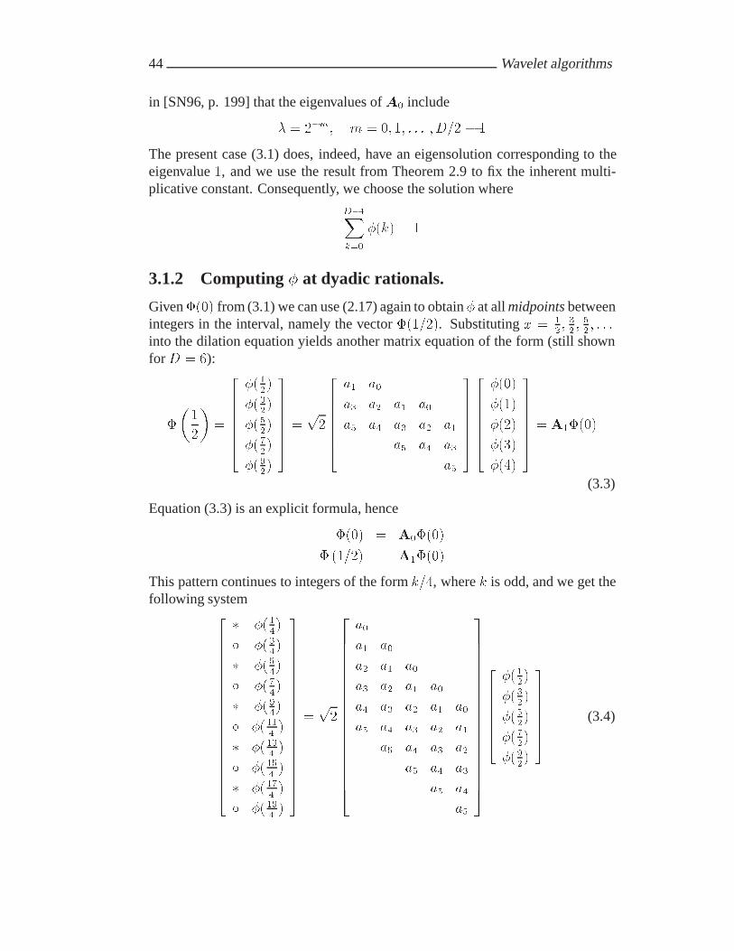
44 Wavelet algorithms
in [SN96, p. 199] that the eigenvalues of A� include
� � ��m� m � �� �� � � � �D�� � �
The present case (3.1) does, indeed, have an eigensolution corresponding to theeigenvalue �, and we use the result from Theorem 2.9 to fix the inherent multi-plicative constant. Consequently, we choose the solution where
D��Xk��
��k� � �
3.1.2 Computing � at dyadic rationals.
Given���� from (3.1) we can use (2.17) again to obtain � at all midpoints betweenintegers in the interval, namely the vector ������. Substituting x � �
�� ��� ��� � � �
into the dilation equation yields another matrix equation of the form (still shownfor D � �):
�
�
�
�
�������
�����
�����
�����
�����
�����
������� �
p�
�������
a� a�
a� a� a� a�
a� a� a� a� a�
a� a� a�
a�
�������
�������
����
����
����
����
����
������� � A�����
(3.3)
Equation (3.3) is an explicit formula, hence
���� � A�����
� ����� � A�����
This pattern continues to integers of the form k��, where k is odd, and we get thefollowing system�
������������������
� �����
� �����
� �����
� �����
� �����
� ����� �
� ����� �
� ����� �
� ����� �
� ������
�������������������
�p�
�������������������
a�
a� a�
a� a� a�
a� a� a� a�
a� a� a� a� a�
a� a� a� a� a�
a� a� a� a�
a� a� a�
a� a�
a�
�������������������
�������
�����
�����
�����
�����
�����
������� (3.4)
3.1 Numerical evaluation of � and � 45
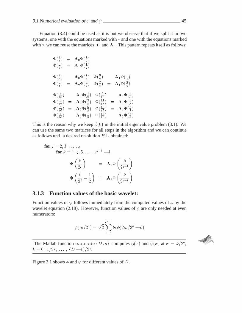
Equation (3.4) could be used as it is but we observe that if we split it in twosystems, one with the equations marked with � and one with the equations markedwith �, we can reuse the matricesA� andA�. This pattern repeats itself as follows:
����� � A������
����� � A���
���
����� � A������ ���
�� � A���
���
����� � A���
��� ���
�� � A���
���
�� �� � � A���
��� �� �
� � � A���
���
�� �� � � A���
��� ����
� � � A���
���
�� �� � � A���
��� ����
� � � A���
���
�� �� � � A���
��� ����� � � A���
���
This is the reason why we keep ���� in the initial eigenvalue problem (3.1): Wecan use the same two matrices for all steps in the algorithm and we can continueas follows until a desired resolution �q is obtained:
for j � �� �� � � � � qfor k � �� �� �� � � � � �j�� � �
�
k
�j
� A��
k
�j��
�
k
�j�
�
�
� A��
k
�j��
3.1.3 Function values of the basic wavelet:
Function values of � follows immediately from the computed values of � by thewavelet equation (2.18). However, function values of � are only needed at evennumerators:
��m��q� �p�D��Xk��
bk���m��q � k�
The Matlab function cascade(D,q) computes ��x� and ��x� at x � k��q ,k � �� ���q� � � � � �D � ����q .
Figure 3.1 shows � and � for different values of D.

46 Wavelet algorithms
0 1 2 3−0.5
0
0.5
1
1.5φ, D = 4
0 1 2 3−1
−0.5
0
0.5
1
1.5ψ, D = 4
0 1 2 3 4 5−0.5
0
0.5
1
1.5φ, D = 6
0 1 2 3 4 5−1
−0.5
0
0.5
1
1.5ψ, D = 6
0 2 4 6 8 10−0.5
0
0.5
1
1.5φ, D = 10
0 2 4 6 8 10−1
−0.5
0
0.5
1ψ, D = 10
0 5 10 15 20−0.5
0
0.5
1φ, D = 20
0 5 10 15 20
−0.6
−0.3
0
0.3
0.6ψ, D = 20
0 10 20 30 40−0.5
0
0.5
1φ, D = 40
0 10 20 30 40−0.6
−0.3
0
0.3
0.6ψ, D = 40
Figure 3.1: Basic scaling functions and wavelets plotted for D � �� �� ��� ��� ��.

3.2 Evaluation of scaling function expansions 47
3.2 Evaluation of scaling function expansions
3.2.1 Nonperiodic case
Let � be the basic scaling function of genus D and assume that � is known at thedyadic rationals m��q , m � �� �� � � � � �D � ���q , for some chosen q � N. Wewant to compute the function
f�x� ��X
l���cj�l�j�l�x� (3.5)
at the grid points
x � xk � k��r� k � Z (3.6)
where r � N corresponds to some chosen (dyadic) resolution of the real line.Using (2.6) we find that
�j�l�k��r� � �j�����j�k��r�� l�
� �j�����j�rk � l�
� �j������j�q�rk � �ql���q�
� �j����m�k� l���q� (3.7)
where
m�k� l� � k�j�q�r � l�q (3.8)
Hence, m�k� l� serves as an index into the vector of pre-computed values of �. Forthis to make sense m�k� l� must be an integer, which leads to the restriction
j � q � r � � (3.9)
Only D� � terms of (3.5) can be nonzero for any given xk. From (3.7) we seethat these terms are determined by the condition
� �m�k� l�
�q� D � �
Hence, the relevant values of l are l � l��k�� l��k� � �� � � � � l��k� �D � �, where
l��k� ��k�j�r
��D � � (3.10)
The sum (3.5), for x given by (3.6), can therefore be written as
f
k
�r
� �j��
l��k��D��Xl�l��k�
cj�l�
m�k� l�
�q
� k � Z (3.11)

48 Wavelet algorithms
3.2.2 Periodic case
We want to compute the function
f�x� ��j��Xl��
cj�l ��j�l�x�� x � �� �� (3.12)
for x � xk � k��r� k � �� �� � � � � �r � � where r � N. Hence we have
f
k
�r
�
�j��Xl��
cj�l ��j�l
k
�r
��j��Xl��
cj�lXn�Z
�j�l
k
�r� n
� �j���j��Xl��
cj�lXn�Z
�
m�k� l� � �j�qn
�q
with m�k� l� � k�j�q�r � l�q by the same manipulation as in (3.7). Now, as-suming that j � J� where J� is given by (2.47) we have �j � D � �. UsingLemma 3.1 (proved below), we obtain the expression
f
k
�r
� �j��
�j��Xl��
cj�l�
hm�k� l�i�j�q�q
� k � �� �� � � � � �r � � (3.13)
Lemma 3.1 Let � be a scaling function with support ��D��� and letm�n� j� q �Z with q � � and �j � D � �. Then
�Xn���
�
m� �j�qn
�q
� �
hmi�j�q�q
Proof: Since �j � D � �, only one term of the sum contributes to the result andthere exists a unique n � n� such that
m� �j�qn�
�q� �� �j�
Then we know that m� �j�qn� � �� �j�q� but this interval is precisely the rangeof the modulus operator defined in Appendix B, so
m� �j�qn� � hm� �j�qni�j�q � hmi�j�q � n � Zfrom which the result follows. �

3.2 Evaluation of scaling function expansions 49
3.2.3 DST and IDST - matrix formulation
Equation (3.13) is a linear mapping from �j scaling function coefficients to �r
samples of f , so it has a matrix formulation. Let cj � cj��� cj��� � � � � cj��j���T andf r � f���� f����r�� � � � � f���r � ����r��T . We denote the mapping
f r � T r�jcj (3.14)
When r � j then (3.14) becomes
f j � T j�jcj (3.15)
T j�j is a square matrix of order N � �j . In the case of (3.15) we will often dropthe subscripts and write simply
f � Tc (3.16)
This has the form (shown here for j � �, D � �)
�BBBBBBBBBBBBB�
f��
f���
f���
f���
f���
f���
f� �
f���
�CCCCCCCCCCCCCA
� ���
�BBBBBBBBBBBBB�
��� ��� ���
��� ��� ���
��� ��� ���
��� ��� ���
��� ��� ���
��� ��� ���
��� ��� ���
��� ��� ���
�CCCCCCCCCCCCCA
�BBBBBBBBBBBBB�
c���
c���
c���
c���
c���
c���
c��
c���
�CCCCCCCCCCCCCA
Note that only values of � at the integers appear in T . The matrix T is non-singular and we can write
c � T��f (3.17)
We denote (3.17) the discrete scaling function transform (DST)1 and (3.16) theinverse discrete scaling function transform (IDST) .
The Matlab function dst(f,D) computes (3.17) and idst(c,D) computes(3.16).
1DST should not be confused with the discrete sine transform.

50 Wavelet algorithms
We now consider the the computational problem of interpolating a functionf � C��� ��� between samples at resolution r. That is, we want to use the functionvalues f�k��r�� k � �� �� � � � � �r � � to compute approximations to f�k��r
�
�� k ��� �� � � � � �r
� � � for some r� � r. There are two steps. The first is to solve thesystem
T r�rcr � f r
for cr. The second is to compute the vector fr� defined by
f r� � T r��rcr (3.18)
Equation (3.18) is illustrated below for the case r � �� r� � �.
�BBBBBBBBBBBBBBBBBBBBBBBBBBBBBBBBB�
f��
f� ��
f� ��
f� ��
f� ��
f� ��
f� �
f� ��
f� ��
f� ��
f����
f����
f����
f����
f����
f����
�CCCCCCCCCCCCCCCCCCCCCCCCCCCCCCCCCA
� ���
�BBBBBBBBBBBBBBBBBBBBBBBBBBBBBBBBB�
��� ��� ���
���� ���� ����
��� ��� ���
���� ���� ����
��� ��� ���
���� ���� ����
��� ��� ���
���� ���� ����
��� ��� ���
���� ���� ����
��� ��� ���
���� ���� ����
��� ��� ���
���� ���� ����
��� ��� ���
���� ���� ����
�CCCCCCCCCCCCCCCCCCCCCCCCCCCCCCCCCA
�BBBBBBBBBB�
c���c���c���c���c���c���c�� c���
�CCCCCCCCCCA
Figure 3.2 show how scaling functions can interpolate between samples of asine function.
3.2.4 Periodic functions on the interval �a� b�
Consider the problem of expressing a periodic function f defined on the intervala� b�, where a� b � R instead of the unit interval. This can be accomplished bymapping the interval a� b� linearly to the unit interval and then use the machineryderived in Section 3.2.3.

3.2 Evaluation of scaling function expansions 51
0 1 2 3 4 5 6−1
−0.5
0
0.5
1D = 4, Error = 0.14381
0 1 2 3 4 5 6−1
−0.5
0
0.5
1D = 6, Error = 0.04921
0 1 2 3 4 5 6−1
−0.5
0
0.5
1D = 8, Error = 0.012534
Figure 3.2: A sine function is sampled in 8 points (r � ). Scaling functions of genusD � �� �� � are then used to interpolate in ��� points (r � � �).
We impose the resolution �r on the interval a� b, i.e.
xk � kb� a
�r� a� k � �� �� � � � � �r � �
The linear mapping of the interval a � x � b to the interval � � y � � is givenby
y �x� a
b� a� a � x � b
hence yk � k��r� k � �� �� � � � � �r � � . Let
g�y� � f�x� � f��b� a�y � a�� � � y � �
52 Wavelet algorithms
Then we have from (3.13)
g�yk� � g�k��r� � �j���j��Xl��
cj�l�
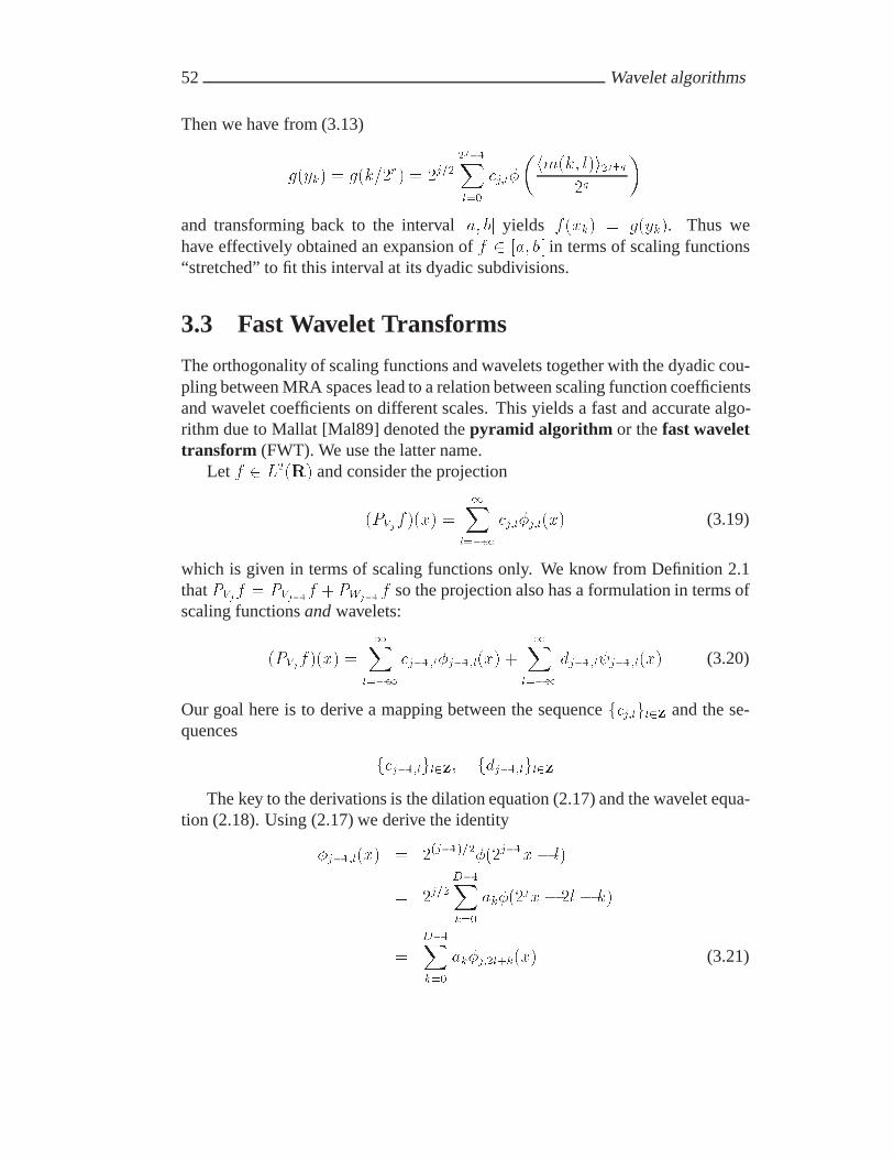
hm�k� l�i�j�q�q
and transforming back to the interval a� b yields f�xk� � g�yk�. Thus wehave effectively obtained an expansion of f � a� b in terms of scaling functions“stretched” to fit this interval at its dyadic subdivisions.
3.3 Fast Wavelet Transforms
The orthogonality of scaling functions and wavelets together with the dyadic cou-pling between MRA spaces lead to a relation between scaling function coefficientsand wavelet coefficients on different scales. This yields a fast and accurate algo-rithm due to Mallat [Mal89] denoted the pyramid algorithm or the fast wavelettransform (FWT). We use the latter name.
Let f � L��R� and consider the projection
�PVjf��x� �
�Xl���
cj�l�j�l�x� (3.19)
which is given in terms of scaling functions only. We know from Definition 2.1that PVjf � PVj��f �PWj��f so the projection also has a formulation in terms ofscaling functions and wavelets:
�PVjf��x� ��X
l���cj���l�j���l�x� �
�Xl���
dj���l�j���l�x� (3.20)
Our goal here is to derive a mapping between the sequence fcj�lgl�Z and the se-quences
fcj���lgl�Z� fdj���lgl�ZThe key to the derivations is the dilation equation (2.17) and the wavelet equa-
tion (2.18). Using (2.17) we derive the identity
�j���l�x� � ��j��������j��x� l�
� �j��D��Xk��
ak���jx� �l � k�
�D��Xk��
ak�j��l�k�x� (3.21)

3.3 Fast Wavelet Transforms 53
and from (2.18) we have
�j���l�x� �D��Xk��
bk�j��l�k�x� (3.22)
Substituting the first identity into the definition of cj�l (2.12) we obtain
cj���l �
Z �
��f�x�
D��Xk��
ak�j��l�k�x� dx
�
D��Xk��
ak
Z �
��f�x��j��l�k�x� dx
�D��Xk��
akcj��l�k
and similarly for dj���l. Thus, we obtain the relations
cj���l �
D��Xk��
akcj��l�k (3.23)
dj���l �D��Xk��
bkcj��l�k (3.24)
which define a linear mapping from the coefficients in (3.19) to the coefficientsin (3.20). We will refer to this as the partial wavelet transform (PWT) . To de-compose the space Vj further, one applies the mapping to the sequence fcj���lgl�Zto obtain the new sequences fcj���lgl�Z and fdj���lgl�Z. This pattern can be fur-ther repeated yielding the full FWT: Applying (3.23) and (3.24) recursively forj � J� J � �� � � � � J� � �, starting with the initial sequence fcJ�lgl�Z, will thenproduce the wavelet coefficients in the expansion given in (2.13). Note that oncethe elements dj���l have been computed, they are not modified in subsequent steps.This means that the FWT is very efficient in terms of computational work.
The inverse mapping can be derived in a similar fashion. Equating (3.19) with(3.20) and using (3.21), (3.22) again we get�X
l���cj�l�j�l�x� �
�Xn���
cj���n�j���n�x� ��X
n���dj���n�j���n�x�
��X
n���cj���n
D��Xk��
ak�j��n�k�x� ��X
n���dj���n
D��Xk��
bk�j��n�k�x�
�D��Xk��
�Xn���
cj���nak � dj���nbk��j��n�k�x�

54 Wavelet algorithms
We now introduce the variable l � �n�k in the last expression. Since k � l��nand k � ��D � ��, we find for given l the following bounds on n:�
l�D � �
�
� n��l� � n � n��l�
l
�
!(3.25)
Hence
�Xl���
cj�l�j�l�x� ��X
l���
n��l�Xn�n��l�
cj���nal��n � dj���nbl��n��j�l�x�
and equating coefficients we obtain the reconstruction formula
cj�l �
n��l�Xn�n��l�
cj���nal��n � dj���nbl��n (3.26)
We will call this the inverse partial wavelet transform (IPWT). Consequently,the inverse fast wavelet transform (IFWT) is obtained by repeated applicationof (3.26) for j � J� � �� J� � �� � � � � J .
3.3.1 Periodic FWT
If the underlying function f is periodic we also have periodicity in the scalingfunction and wavelet coefficients; cj�l � cj�l��jp by (2.60) and dj�l � dj�l��jp by(2.59). Hence, it is enough to consider �j coefficients of either type at level j. Theperiodic PWT is thus
cj���l �
D��Xk��
akcj�h�l�ki�j (3.27)
dj���l �D��Xk��
bkcj�h�l�ki�j (3.28)
where
l � �� �� � � � � �j�� � �
Hence the periodic FWT is obtained by repeated application of (3.27) and (3.28)for j � J� J � �� � � � � J� � �.
If we let J� � � then (3.27) and (3.28) can be applied until all coefficientsin the (canonical) expansion (2.54) have been computed. There is then only onescaling function coefficient left, namely c��� (the “DC” term), the rest will bewavelet coefficients. Figure 3.3 shows an example of the periodic FWT.

3.3 Fast Wavelet Transforms 55
c���c���c���c���c���c���c�� c���c���c���c����c����c����c����c����c����
� c���c���c���c���c���c���c�� c���d���
d���
d���
d���
d���
d���
d��
d���
� c���c���c���c���d���
d���
d���
d���
d���
d���
d���
d���
d���
d���
d��
d���
� c���c���d���
d���
d���
d���
d���
d���
d���
d���
d���
d���
d���
d���
d��
d���
� c���d���
d���
d���
d���
d���
d���
d���
d���
d���
d���
d���
d���
d���
d��
d���
Figure 3.3: The periodic FWT. The shaded elements dj�l obtained at each level remainthe same at subsequent levels. Here the depth is taken to be as large as possible, i.e.� � J � �.

56 Wavelet algorithms
The reconstruction algorithm (IPWT) for the periodic problem is similar to thenon-periodic version:
cj�l �
n��l�Xn�n��l�
cj���hni�j��al��n � dj���hni�j�� bl��n (3.29)
with n��l� and n��l� defined as in (3.25) and
l � �� �� � � � � �j � �
Hence the periodic IFWT is obtained by applying (3.29) for j � J� � �� J� ��� � � � � J . We restrict ourselves to algorithms for periodic problems throughoutthis report. Hence we will consider only the periodic cases of FWT, PWT, IFWT,and IPWT.
3.3.2 Matrix representation of the FWT
Let cj � cj��� cj��� � � � � cj��j���T and similarly, dj � dj��� dj��� � � � � dj��j���T .Since (3.27) and (3.28) are linear mappings from R�j onto R�j��
the PWT canbe represented as
cj�� � Ajcj
dj�� � Bjcj
where Aj and Bj are �j�� by �j matrices containing the filter coefficients. ForD � � and j � � we have
A� �
"BBBBBBBBBB#
a� a� a� a� a� a�a� a� a� a� a� a�
a� a� a� a� a� a�a� a� a� a� a� a�
a� a� a� a� a� a�a� a� a� a� a� a�
a� a� a� a� a� a�a� a� a� a� a� a�
$CCCCCCCCCCA
and
B� �
"BBBBBBBBBB#
b� b� b� b� b� b�b� b� b� b� b� b�
b� b� b� b� b� b�b� b� b� b� b� b�
b� b� b� b� b� b�b� b� b� b� b� b�
b� b� b� b� b� b�b� b� b� b� b� b�
$CCCCCCCCCCA

3.3 Fast Wavelet Transforms 57
These are shift-circulant matrices (see Definition 8.1). Moreover, the rows are or-thonormal by equations (2.22) and (2.23):
Pk akak��n � ��n and
Pk bkbk��n �
��n. Bj is similar, but with bk’s in place of ak’s; hence the rows of Bj are alsoorthonormal. Moreover, the inner product of any row inAj with any row in Bj iszero by Theorem 2.1, i.e. AjB
Tj � �.
We now combine Aj and Bj to obtain a �j � �j matrix
Qj �
�Aj
Bj
�
which represents the combined mapping�cj��dj��
�� Qjcj (3.30)
Equation (3.30) is the matrix representation of a PWT step as defined by (3.27)and (3.28). The matrix Qj is orthogonal since
QjQTj �
�Aj
Bj
�AT
j BTj � �
�AjA
Tj AjB
Tj
BjATj BjB
Tj
��
�I j �� Ij
�
Hence the mapping (3.30) is inverted by
cj � QTj
�cj��dj��
�(3.31)
Equation (3.31) is the matrix representation of an IPWT step as defined in (3.29).The FWT from level J to level J� � J � � can now be expressed as the
matrix-vector product
d �W �c (3.32)
where c � cJ ,
d �
"BBBBB#
cJ�dJ�dJ���
...dJ��
$CCCCCA
and
W � � QJ�QJ��� � � � QJ��QJ �

58 Wavelet algorithms
The matrix Qj , of order �J , is given by
Qj �
����������������
Qj
Ik�j�J�
����������������
where Ik�j�J� denotes the k � k identity matrix with k � k�j� J� � �J � �j . Itfollows that W � is orthogonal2 and hence the IFWT is given by
c ��W �
�Td
3.3.3 A more general FWT
Suppose that elements to be transformed may contain other prime factors than�, i.e. N � K�J , with J�K � Z and hKi� � �. In this case, the FWT canstill be defined by mappings of the form (3.27) and (3.28) with a maximal depth� � J , i.e. J� � �. It will be convenient to use a slightly different notation for thealgorithms in Chapters 5, 6, and 8. Hence, let Si � N��i and
cik cJ�i�kdik dJ�i�k
for i � �� �� � � � � � � � and k � �� �� � � � � Si � �. We can now define the FWT asfollows:
Definition 3.1 Fast wavelet transform (FWT)Let J�K � N with hKi� � � and N � K�J . Let c� � fc�kgN��k�� be given. TheFWT is then computed by the recurrence formulas
ci��n �D��Xl��
alcihl��niSi
di��n �
D��Xl��
blcihl��niSi
(3.33)
where i � �� �� � � � � �� �, Si � N��i, and n � �� �� � � � � Si�� � �.
2The orthonormality ofW � is one motivation for the choice of dilation equations mentionedin Remark 2.4.

3.3 Fast Wavelet Transforms 59
The relation between the scaling function coefficients and the underlying func-tion is unimportant for the FWT algorithm per se: In numerical applications weoften need to apply the FWT to vectors of function values or even arbitrary vec-tors. Hence let x � RN . Then the expression
�x �W �x (3.34)
is defined by putting c� � x, performing � steps of of (3.33), and letting
�x �nfc�kgS���k�� � ffdikgSi��k�� gi������� ��
o
If � is omitted in (3.34) it will assume its maximal value J . Note that W � � I
for � � �. The IFWT is written similarly as
x � �W ��T �x (3.35)
corresponding to the recurrence formula
cil �
n��l�Xn�n��l�
ci��hniSi��al��n � di��hniSi��
bl��n
where i � �� �� � � �� � � � � �� �, Si � N��i, l � �� �� � � � � Si � �, and n��l� andn��l� are defined as in (3.25).
The Matlab functionfwt(x, D, �) computes (3.34) andifwt(�x, D, �) computes(3.35).
3.3.4 Complexity of the FWT algorithm
One step of (3.33), the PWT, involvesDSi additions andDSi multiplications. Thenumber of floating point operations is therefore
FPWT�Si� � �DSi (3.36)
Let N be the total number of elements to be transformed and assume that theFWT is carried out to depth �. The FWT consists of � applications of the PWT to

60 Wavelet algorithms
successively shorter vectors so the total work is
FFWT�N� ����Xi��
FPWT
N
�i
����Xi��
�DN
�i
� �DN� � �
��
� � ��
� �DN
� � �
��
� �DN (3.37)
D is normally constant throughout wavelet analysis, so the complexity is O�N�.The IFWT has the same complexity as the FWT. For comparison we mention thatthe complexity of the fast Fourier transform (FFT) is O�N log�N�.
3.3.5 2D FWT
Using the definition of W � from the previous section, we define the 2D FWT as�X �W �MX�W �N �T (3.38)
whereX� �X � RM�N . The parameters �M and �N are the transform depths in thefirst and second dimensions, respectively. Equation (3.38) can be expressed as M1D wavelet transforms of the rows of X followed by N 1D wavelet transformsof the columns of X�W �N �T , i.e.
�X �W �M�W �NXT
�TTherefore it is straightforward to compute the 2D FWT given the 1D FWT fromDefinition 3.1. It follows that the inverse 2D FWT is defined as
X ��W �M
�T �XW �N (3.39)
The Matlab function fwt2(X, D, �M , �N ) computes (3.38) and ifwt2( �X, D,�M , �N ) computes (3.39).
Using (3.37) we find the computational work of the 2D FWT as follows
FFWT2�M�N� � M FFWT�N� �N FFWT�M�
� M�DN
� � �
��N
�N�DM
� � �
��M
� �DMN
� � �
��M� �
��N
� �DMN (3.40)
The computational work of the inverse 2D FWT is the same.

Chapter 4
Approximation properties
4.1 Accuracy of the multiresolution spaces
4.1.1 Approximation properties of VJWe will now discuss the pointwise approximation error introduced when f is ap-proximated by an expansion in scaling functions at level J . Let J � Z, f � L��R�and assume that f is P times differentiable everywhere.
For an arbitrary, but fixed x, we define the pointwise error as
eJ�x� � f�x�� �PVJf��x�� x � Rwhere �PVJf��x� is the orthogonal projection of f onto the approximation spaceVJ as defined in Section 2.1.
Recall that PVJf has expansions in terms of scaling functions as well as interms of wavelets. The wavelet expansion for PVJf is
�PVJf� �x� ��X
k���cJ��k�J��k�x� �
J��Xj�J�
�Xk���
dj�k�j�k�x� (4.1)
and by letting J �� temporarily we get a wavelet expansion for f itself:
f�x� �
�Xk���
cJ��k�J��k�x� �
�Xj�J�
�Xk���
dj�k�j�k�x� (4.2)
Then, subtracting (4.2) from (4.1) we obtain an expression for the error eJ in termsof the wavelets at scales j � J :
eJ�x� ��Xj�J
�Xk���
dj�k�j�k�x� (4.3)

62 Approximation properties
Define
C� � maxx�Ij�k
�����jx� k��� � max
y����D���j��y�j
Hence maxx�Ij�k j�j�k�x�j � �j��C� and using Theorem 2.5, we find that
jdj�k�j�k�x�j � CP��jP max
��Ij�k
��f �P ������ C�
Recall that
supp��j�k� � Ij�k �
�k
�j�k �D � �
�j
�Hence, there are at most D � � intervals Ij�k containing a given value of x. Thusfor any x only D� � terms in the inner summation in (4.3) are nonzero. Let Ij bethe union of all these intervals, i.e.
Ij�x� ��
fl�x�Ij�lgIj�l
and let
�Pj �x� � max��Ij�x�
��f �P ������Then one finds a common bound for all terms in the inner sum:
�Xk���
jdj�k�j�k�x�j � C�CP��jP �D � ���Pj �x�
The outer sum can now be evaluated using the fact that
�PJ �x� � �PJ���x� � �PJ���x� � � � �and we establish the bound
jeJ�x�j � C�CP �D � ���PJ �x��Xj�J
��jP
� C�CP �D � ���PJ �x���JP
�� ��P
Thus we see that that for an arbitrary but fixed x the approximation error will bebounded as
jeJ�x�j � O���JP �
This is exponential decay with respect to the resolution J . Furthermore, thegreater the number of vanishing moments P , the faster the decay.
Finally, note that each error term dj�k�j�k�x� is zero for x �� Ij�k. This meansthat eJ�x� depends only on f�y�� y � x� x� �D� ����J ��. This is what was alsoobserved in Chapter 1.

4.1 Accuracy of the multiresolution spaces 63
4.1.2 Approximation properties of �VJ
We now consider the approximation error in the periodic case. Let f � L���� ���and assume that its periodic extension (2.55) is P times differentiable everywhere.Furthermore, let J � J� where J� is given as in (2.47) and define the approxima-tion error as
�eJ�x� � f�x�� �PVJf��x�� x � �� ��
where �PVJf��x� is the orthogonal projection of f onto the approximation space
�VJ as defined in Definition 2.4.Using the periodic wavelet expansion (2.53) and proceeding as in the non-
periodic case we find that
�eJ�x� �
�Xj�J
�j��Xk��
dj�k ��j�k�x� (4.4)
Since the coefficients dj�k are the same as in the non-periodic case by (2.58),Theorem (2.5) applies and we can repeat the analysis from Section 4.1.1 and,indeed, we obtain that
j�eJ�x�j � O���JP �� x � �� ��
We will now consider the infinity norm of �eJ defined by
k�eJk� � maxx������
j�eJ�x�j
A similar analysis as before yields
k�eJk� ��Xj�J
�j��Xk��
jdj�kj maxx�Ij�k
��� ��j�k�x����
� C�CP
�Xj�J
�j��Xk��
�j����j�P��� � max
��Ij�k
��f �P ������� C�CP max
�������
��f �P ������ �Xj�J
��jP
� C�CP max�������
��f �P ������ ��JP
�� ��P
Hence
k�eJk� � O���JP �
64 Approximation properties
Finally, consider the 2-norm of �eJ :
k�eJk�� �Z �
�
�e�J�x� dx �Z �
�
k�eJk�� dx � k�eJk��Z �
�
dx � k�eJk��
hence we have also in this case
k�eJk� � O���JP � (4.5)
4.2 Wavelet compression errors
In this Section we will see how well a function f � �VJ is approximated by awavelet expansion where small wavelet coefficients have been discarded. We willrestrict attention to the case of the interval �� ��.
It was shown in Section 2.1.6 that the wavelet coefficients corresponding to aregion where f is smooth decay rapidly and are not affected by regions where f isnot so smooth. We now investigate the error committed when small wavelet coeffi-cients are discarded. We will refer to those as the insignificant wavelet coefficientswhile those remaining will be referred to as the significant wavelet coefficients.These definitions are rendered quantitative in the following.
Let � be a given threshold for separating the insignificant wavelet coefficientsfrom the significant ones. We define an index set identifying the indices of thesignificant wavelet coefficients at level j:
T �j �
%k � � � k � �j � � � jdj�kj � �
&Hence the indices of the insignificant coefficients are given by
R�j � T �
j n T �j
With this notation we can write an �-truncated wavelet expansion for f as follows
�PVJ
f���x� �
�J���Xk��
cJ��k��J��k�x� �
J��Xj�J�
Xk�T �j
dj�k ��j�k�x� (4.6)
Let Ns��� be the number of all significant wavelet coefficients, i.e.
Ns��� �J��Xj�J�
�T �j � �J�
where � denotes the cardinality of T �j . The last term corresponds to the scaling
function coefficients that must be present in the expansion because they provide

4.2 Wavelet compression errors 65
the coarse approximation on which the wavelets build the fine structures. If we letN � �J be the dimension of the finest space �VJ then we can define the symbol Nr
to be the number of insignificant coefficients in the wavelet expansion, i.e.
Nr��� � N �Ns���
We then define the error introduced by this truncation as
�e�J�x� � PVJf � �
PVJf��
�J��Xj�J�
Xk�R�
j
dj�k�j�k�x�
with the number of terms being equal toNr���. The 2-norm of �e�J�x� is then foundas
k�e�J�x�k�� �
''''''J��Xj�J�
Xk�R�
j
dj�k�j�k�x�
''''''�
�
�J��Xj�J�
Xk�R�
j
jdj�kj�
� ��Nr���
so whenever the threshold is � then
k�e�J�x�k� � �pNr��� (4.7)
For the infinity norm the situation is slightly different. For reasons that willsoon become clear we now redefine the index set as
T �j �
%k � � � k � �j � � � jdj�kj � ���j��
&and R�
j � T �j n T �
j . Note that we now modify the threshold according to the scaleat which the wavelet coefficient belongs. Applying the infinity norm to �e�J with

66 Approximation properties
the new definition of Tj yields
k�e�J�x�k� �J��Xj�J�
Xk�R�
j
maxx
�jdj�k�j�k�x�j�
� C�
J��Xj�J�
Xk�R�
j
jdj�kj �j��
� C�
J��Xj�J�
Xk�R�
j
�
� C��Nr���
so whenever the threshold is � then
k�e�J�x�k� � C��Nr��� (4.8)
The difference between (4.7) and (4.8) lies first and foremost in the fact that thethreshold is scaled in the latter case. This means that the threshold essentially de-creases with increasing scale such that more wavelet coefficients will be includedat the finer scales. Hence Nr��� will tend to be smaller for the �-norm than forthe �-norm.
Remark 4.1 A heuristic way of estimating Ns is given as follows: Let f�x� be asmooth function with one singularity located at x � xs. Then dj�k � � for those jand k where xs � Ij�k. Hence we have D � � significant coefficients at each levelyielding a total of ��D � ��. Hence if f has q singularities we can estimate Ns tobe roughly proportional to
q��D � ��
4.3 Scaling function coefficients or function values ?
It was mentioned in Section 3.3.3 that the fast wavelet transform can be applieddirectly to sequences of function values instead of scaling function coefficients.Since this is often done in practice (see, for example, [SN96, p. 232]), yet rarelyjustified, we consider it here.
Suppose that f � L��R� is approximately constant on the interval IJ�l givenby (2.21), a condition that is satisfied if J is sufficiently large since the length of

4.4 A compression example 67
IJ�l is �D � ����J . Then f�x� � f�l��J � for x � IJ�l and we find that
cJ�l � �J��ZIJ�l
f�x����Jx� l� dx
� �J��f�l��J �
ZIJ�l
���Jx� l� dx
� ��J��f�l��J �Z D��
�
��y� dy
or
cJ�l � ��J��f�l��J �
In vector notation this becomes
c � ��J��f
and from (3.32) follows
d � ��J��Wf (4.9)
Hence, the elements in �f � Wf behave approximately like those in d (exceptfor the constant factor) when J is sufficiently large.
4.4 A compression example
One of the most successful applications of the wavelet transform is image com-pression. Much can be said about this important field, but an exhaustive accountwould be far beyond the scope of this thesis. However, with the wavelet theorydeveloped thus far we can give a simple but instructive example of the principlesbehind wavelet image compression. For details, we refer to [Chu97, SN96, H�94,VK95] among others.
Let X be an M � N matrix representation of a digital image. Each elementof X corresponds to one pixel with its value corresponding to the light intensity.Figure 4.1 shows an example of a digital image encoded in X .
Applying the 2D FWT from (3.38) to X yields
�X �W �MX�W �N
�Twhich is shown in Figure 4.2 with D � �. The upper left block is a smoothedapproximation of the original image. The other blocks represent details at various

68 Approximation properties
Figure 4.1: A digital imageX . Here M � � �� N � ��.
Figure 4.2: The wavelet spectrum �X . Here �M � �N � and D � �.

4.4 A compression example 69
Figure 4.3: Reconstructed image Y . Compression ratio � � ���.
scales and it can be seen that the significant elements are located where the orig-inal image has edges. The large smooth areas are well represented by the coarseapproximation so no further details are needed there.
Assuming that the image is obtained as function values of some underlyingfunction which has some smooth regions we expect many of the elements in �Xto be small. The simplest compression strategy is to discard small elements in �X ,and for this purpose we define
�X� � trunc� �X� �� � f �X�m�n�
��� �X�m�n
��� � �g
By inverse FWT one obtains the approximation
Y ��W �M
�T �X�W �N
which is shown in Figure 4.3. The threshold � has been chosen such that only ��of the wavelet coefficients are retained in �X
�. This gives the error
EFWT �kY �Xk�kXk�
� ���� � ����
We point out that there is no norm that accurately reflects the way people perceivethe error introduced when compressing an image. The only reliable measure is thesubjective impression of the image quality [Str92, p. 364]. Attempts at “objective”

70 Approximation properties
Figure 4.4: Reconstructed image F T �X�F .
error measurement customarily make use of the peak signal-to-noise ratio (PSNR)which is essentially based on the �-norm [Chu97, p. 180], [JS94, p. 404].
In order to assess the merits of the procedure described above, we now repeatit with the discrete Fourier transform (DFT): Using the Fourier matrixF N definedin (C.3) in place of W we get
X � FMXFTN
Retaining �� of the elements in X as before and transforming back yields theimage shown in Figure 4.4. The discarded elements in this case correspond tohigh frequencies so the compressed image becomes blurred. The correspondingrelative error is now
EDFT � ���� � ����
In practical applications one does not use the DFT on the entire image. Rather,the DFT is applied to smaller blocks which are then compressed separately. How-ever, this approach can lead to artefacts at the block boundaries which degradeimage quality. In any case, this example serves to illustrate why the wavelet trans-form is an attractive alternative to the Fourier transform; edges and other localizedsmall scale features are added where needed, and omitted where they are not. Thisis all a direct consequence of Theorem 2.5.
Finally, we mention that a practical image compression algorithm does muchmore than merely throw away small coefficients. Typically, more elaborate trun-cation (quantization) schemes are combined with entropy coding to minimize theamount of data needed to represent the signal [Chu97, Str92, H�94].
Part II
Fast Wavelet Transforms onSupercomputers


Chapter 5
Vectorization of the Fast WaveletTransform
Problems involving the FWT are typically large and wavelet transforms can betime-consuming even though the algorithmic complexity is proportional to theproblem size. The use of high performance computers is one way of speeding upthe FWT.
In this chapter and the next we will describe our efforts to implement the 1Dand the 2D FWT on a selection of high-performance computers, especially theFujitsu VPP300. For simplicity we let K � � (see Definition 3.1) throughoutthese chapters.
The Fujitsu VPP300 is a vector-parallel computer. This means that it consistsof a number of vector processors connected in an efficient network. Good vec-tor performance on the individual processors is therefore crucial to good parallelperformance. In this chapter we discuss the implementation and performance ofthe FWT on one node of the VPP300. In Chapter 6 we discuss parallelization ofthe FWT and report results of the parallel implementation on several nodes on theVPP300. Some of the material presented here has also appeared in [NH95].
5.1 The Fujitsu VPP300
The vector units on the VPP300 run with a clock frequency of ��� MHz. Theycan execute � multiplications and � additions per clock cycle, leading to a peakperformance of ����� Gflop/s per processor. The actual performance, however,depends on many factors such as
1. vector length
2. memory stride

74 Vectorization of the Fast Wavelet Transform
3. arithmetic density
4. ratio of arithmetic operations to load/store operations
5. type of operations
A vector processor is designed to perform arithmetic operations on vectors ofnumbers through hardware pipelining. There is an overhead involved with eachvector instruction, so good performance requires long vector lengths.
As with all modern computers, the memory speed of the VPP falls short of theprocessor speed. To overcome this problem, memory is arranged in banks withconsecutive elements spread across the banks. Stride-one access then means thatthe memory banks have time to recover between consecutive memory accesses sothat they are always ready to deliver a piece of data at the rate at which it is re-quested. Furthermore, the VPP300 has a special instruction for this which is fasterthan any non-uniform memory access. Finally, on computer architectures usingcache, stride-one means that all elements in a cache line will be used before it isflushed. In either case, a stride different from one can lead to poor performancebecause the processor has to wait until the data are ready.
Optimal performance on the VPP300 requires that � multiplications and �additions occur every clock cycle. Therefore, any loop containing only addition ormultiplication can never run faster than half the peak performance. Also, the useof load and store pipes is crucial. The VPP300 has one load and one store pipe, soaddition of two vectors, say, can at best run at 1/4 of the peak performance becausetwo loads are needed at each iteration. Finally, the type of arithmetic operationsis crucial to the performance. For example, a division takes seven cycles on theVPP. Taking all these issues into account, we see that good vector performancerequires operations of the form
for n � � � N � �y�n � a � x�n � b
where a and b are scalars and x and y are vectors of lengthN , withN being large.For details see [Uni96, HJ88].
5.2 1D FWT
The basic operation in the 1D FWT can be written in the form
for n � � � S�� � �w�n � w�n � al � x�hl��niS

5.2 1D FWT 75
N F CPU time (�s) Mflop/s���� ����� ��� ������� ������ ��� ������� ������ ���� ������� ������ ���� �������� ������� ���� �������� ������� ���� �������� ������� ����� ��������� �������� ����� ��������� �������� ����� ��������� �������� ����� ���
Table 5.1: Timings of the FWT. D � ��, N � �J , J � ��� ��� � � � � ��, and � � J .
as defined by the recurrence formulas (3.33). The arithmetic density as well as theratio of arithmetic operations to load/store operations are good. However, mem-ory is accessed with stride-two because of the inherent double shift in the wavelettransform, and indices must be wrapped because of periodicity. Therefore, opti-mal performance is not expected for the 1D FWT.
Our implementation of the FWT on one node of the VPP300 yields the perfor-mance shown in Table 5.1. We make the following observations from Table 5.1:Firstly, the performance is far from optimal even for the largest value of N . Sec-ondly, the performance improves only slowly as N increases. To understand thelatter property we conduct a performance analysis of one step (the PWT) of therecurrence formulas (3.33). Since this is a simple operation on one vector, weassume that the computation time in the vector processor follows the model
T � ts � tvF (5.1)
where F is the number of floating point operations, T is the total execution time,tv is the computation time for one floating point operation in the pipeline, and tsis the startup time. The performance expressed in floating point operations persecond is then
R �F
T(5.2)
Letting F go to infinity results in the theoretically optimal performance
R� limF��
F
T� lim
F��F
ts � tvF�
�
tv(5.3)

76 Vectorization of the Fast Wavelet Transform
Let � � �� �� be the fraction of R� which is achieved for a given problemsize F. Then F is found from (5.2) with R � �R�:
�
tv�
F
ts � tvF
which has the solution
F ��
�� �
tstv
In particular, for � � ��� we find
F��� �tstv
which is another characteristic performance parameter for the algorithm in ques-tion. F can now be expressed in terms of F��� as F � F��� ���� � ��. For ex-ample, to reach 80 % of the maximum performance, a problem size of F � �F���
is required, and F � �F��� is needed to reach 90 %. The parameter F��� cantherefore be seen as a measure of how quickly the performance approaches R�.A large value of F��� means that the problem must be very large in order to getgood performance. Hence we wish F��� to be as small as possible.
In order to estimate the characteristic parameters F��� and R� we use mea-surements of CPU time in the VPP300. Table 5.2 shows the timings of the se-quence of steps needed to compute the full FWT with � � J � ��, N � �J ,and D � �� (the last result in Table 5.1), i.e. the PWT applied succesively tovectors of length S � N�N��� � � � � �. Using these measurements we estimate theparameters ts and tv (in the least squares sense) to be
ts � �� �s and tv � ������� �s
Consequently
�R��PWT � ��� Mflop/s and
�F����PWT � ����� Operations (5.4)
It can be verified that the values predicted by the linear model correspond wellwith those observed in Table 5.2. The execution time of the PWT thus follows themodel
TPWT�S� � ts � tvFPWT�S�
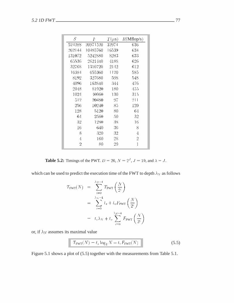
5.2 1D FWT 77
S F T ��s� R�Mflop/s������� �������� ����� ��������� �������� ����� ��������� ������� ���� �������� ������� ���� �������� ������� ���� �������� ������ ���� ������� ������ ��� ������� ������ ��� ������� ����� ��� ������� ����� ��� ������ ����� �� ������ ����� �� ������ ���� �� ���� ���� �� ���� ���� �� ���� ��� �� �� ��� �� �� ��� �� �� �� �� �
Table 5.2: Timings of the PWT. D � ��, N � �J , J � ��, and � � J .
which can be used to predict the execution time of the FWT to depth �N as follows
TFWT�N� �
�N��Xi��
TPWT
N
�i
�
�N��Xi��
ts � tvFPWT
N
�i
� ts�N � tv
�N��Xi��
FPWT
N
�i
or, if �N assumes its maximal value
TFWT�N� � ts log�N � tvFFWT�N� (5.5)
Figure 5.1 shows a plot of (5.5) together with the measurements from Table 5.1.

78 Vectorization of the Fast Wavelet Transform
0 1 2 3 4
x 107
0
2
4
6
x 104
FFWT
TF
WT
Execution time, FWT
Model Measurements
Figure 5.1: The execution time for the FWT plotted as a function of floating pointoperations. The circles are the measured times while the line is the result of the model.
We know from (3.37) that FFWT�N� � �DN . Hence �log�N��FFWT�N� � �for N ��, and we see that the asymptotic performance of the FWT is the sameas that of the PWT:
�R��FWT � �R��PWT ��
tv
However, the equation to be solved for �F����FWT is not linear. Let N��� be thevector length corresponding to �F����FWT. Then �F����FWT � FFWT�N���� ��D�N��� � �� by (3.37) and putting R � R��� (corresponding to � � ���)in (5.2) we get
�R��FWT
��
�F����FWT�N����
TFWT�N����
�
�tv�
�F����FWT
ts log�N��� � tv�F����FWT
tv�F����FWT � ts log�N���
tv�D�N��� � �� � ts log�N���
For the values ts and tv obtained from timings of the PWT we find the estimateN��� � ���� which yields
�F����FWT � �F����PWT log�N��� � ������ operations
This agrees with the observed values in Table 5.1. It is seen, both from the obser-vations and the model, that the value of �F����FWT is very high compared to that
5.3 Multiple 1D FWT 79
of the PWT (5.4). The explanation for this is revealed by the analysis just carriedout: A new vector operation is started up for each PWT so the startup time tscounts log�N times regardless of the vector length; no matter how long the initialvector length N , the PWT will eventually be applied to short vectors.
Like the stride-two memory access, this property is inherent in the full 1DFWT and we conclude that this computation is not particularly suitable for vec-torization. However, if the depth �N is taken to be smaller than J then the ineffi-ciency due to short vector lengths becomes less severe.
5.3 Multiple 1D FWT
Consider a matrix X � RM�N . We assume that X is stored by columns so thatconsecutive elements in each column are located in consecutive positions in mem-ory. Applying the 1D FWT to every column of X leads to inefficient data accessand large F��� as described in the previous section. By applying the FWT to therows of X instead, one can vectorize over the columns such that all elements willbe accessed with stride-one in vectors of length M . We will refer to this pro-cedure as the multiple 1D FWT (MFWT). Applying the MFWT to a matrix Xcorresponds to computing the expression
X�W �N �T (5.6)
whereW �N is defined as in (3.34). Since there areM rows, the number of floatingpoint operations needed are
FMFWT�M�N� � �DMN��� ����N
�(5.7)
The recurrence formulas now take the form
ci��m�n �
D��Xl��
alcim�hl��niSi
di��m�n �D��Xl��
blcim�hl��niSi
(5.8)
where i � �� �� � � � � �N � �, m � �� �� � � � �M � �, and n � �� �� � � � � Si�� � �.Timings for the MFWT with �N � J � ��, N � �J , and D � ��, where only thevectorized dimension M is varied, are shown in Table 5.3.
We will now derive a performance model for this case. Each step of the MFWTapplies a PWT of length Si to the M rows of X . Hence, by (3.36) the number offlops are �DSiM . Vectorization is achieved by putting m into the innermost loopso computations on each column can be assumed to follow the linear model for

80 Vectorization of the Fast Wavelet Transform
M F T ��s� R�Mflop/s��� ������� ����� ����� ������� ����� ����� ������� ����� ������ �������� ����� ������ �������� ����� ������� �������� ����� �������� �������� ����� �������� ��������� ����� ����
Table 5.3: Timings of the MFWT. �N � J � ��, N � �J , D � ��, and M ���� �� � � � � ����.
vectorization (5.1). Hence the execution time for one step of the MFWT (5.8) isSi�ts � �DMtv� and the execution time for the entire MFWT is
TMFWT �
�N��Xi��
N
�i�ts � �DMtv�
� �N
� � �
��N
�ts � �DMtv� (5.9)
The performance is then given by
RMFWT �FMFWT
TMFWT�
�DM
ts � �DMtv
and �R��MFWT � ��tv as usual. However, we observe that the performance mea-sure is independent of the depth �N . The parameter M��� is found by solving
�
�tv�
�DM���
ts � �DM���tv
which has the solution
M��� �ts
�Dtv
Hence
�F����MFWT � �DN
� � �
��N
M���
� �N
�� �
��N
ts�tv

5.4 2D FWT 81
Using (5.9) and the measurements in Table 5.3 we get the new estimates
ts � ���� �s and tv � �������� �s
These estimates are different from those of the 1D case and reflect the fact that theMFWT algorithm performs better on the VPP300. Consequently we now have
�R��MFWT � ����� Gflop/s and
�F����MFWT � �������� Operations
the latter corresponding to a vector length M��� � ���. These values are close tobeing optimal on the VPP300 (recall that the peak performance per processor is����� Gflop/s). Finally, since �F����MFWT grows with N we note that the MFWTis best for matrices with M � N .
5.4 2D FWT
Recall from Section 6.3 that the 2D wavelet transform is defined by the matrixproduct
�X �W �MX�W �N �T (5.10)
The expression X�W �N �T leads to vector operations on vectors of lengthM and stride-one data access as described in Section 5.3. This is not the casefor the expression W �MX , because it consists of a collection of columnwise 1Dtransforms which do not access the memory efficiently as described in Section 5.2.However (5.10) can be rewritten as
�XT��X�W �N �T
�T�W �M �T
yielding the efficiency of the multiple 1D FWT at the cost of one transpose step.We call this the split-transpose algorithm. It consists of the following threestages:
Algorithm 5.1: split-transpose
1. Z �X�W �N �T
2. U � ZT
3. �XT � U�W �M �T

82 Vectorization of the Fast Wavelet Transform
M F T ��s� R�Mflop/s��� ������� ����� ����� ������� ����� ����� �������� ����� ������ �������� ����� ������� �������� ����� ������� �������� ����� �������� ��������� ����� ����
Table 5.4: Timings of 2D FWT (FWT2). �N � J � ��, N � �J , D � ��, andM � ��� �� � � � � ����.
Transposition can be implemented efficiently on a vector processor by accessingthe matrix elements along the diagonals [Heg95], so the 2D FWT retains the goodvector performance of the MFWT. This is verified by the timings in Table 5.4.
Disregarding the time for the transposition step, a simple model for the 2DFWT execution time is
TFWT2�M�N� � TMFWT�M�N� � TMFWT�N�M� (5.11)
where TMFWT is given by (5.9). Figure 5.2 shows predicted execution times versusmeasured execution times, and it is seen that (5.11) predicts the performance ofthe 2D FWT well.
The asymptotic performance �R��FWT2 can now be determined. Using (3.40),(5.2), and (5.11) we get
RFWT2 ��DMN�� � ����M � ����N �
�N�� � ����N ��ts � �DMtv� � �M�� � ����M ��ts � �DNtv�
Assuming that �M � log��M� and �N � log��N� (the maximal depths) and thatM and N are large, this yields the estimate
RFWT2 � �M�N�DMN
ts � tv(5.12)
and letting M �� we obtain
�R��FWT2�N� ��
ts�DN
� tv(5.13)

5.4 2D FWT 83
0 5 10 15
x 107
0
3
6
9
x 104 Execution time, FWT2
FFWT2
TF
WT
2
Model Measurements
Figure 5.2: The measured times for the 2D FWT compared to the performance model( 5.11).
It is seen that if N goes to infinity as well, we obtain the usual expression (��tv),but for the present case, with N � ����, we have from (5.12)
�R��FWT2 � ����� Gflop/s
which is only slightly less than �R��MFWT. Similarly, to find �F����FWT2 for theproblem at hand we use (5.12) and (5.13) to get the equation
�DN
ts � �DNtv�
�M����N
�DM���Nts � tv
From this we find
M��� �ts
�Dtv � ts�N� ��
corresponding to �F����FWT2 � ������ � ���. It is seen that this value is veryclose to that of the MFWT despite the fact that the transposition step was includedin the measured execution times. However, the corresponding vector length M���
is much smaller as can also be seen in Table 5.4. The reason for this is the factthat where the MFWT suffers from short vector lengths when M is small, the 2DFWT suffers only in stage � of the split-transpose algorithm (5.1). Stage � willvectorize over N and yield good performance in this case. We see that the 2DFWT performs very well indeed on the VPP300, even for rectangular matrices.

84 Vectorization of the Fast Wavelet Transform
5.5 Summary
The FWT has been implemented on the VPP 300. The one-dimensional versionhas a relatively high value of N��� and stride-two memory access so the perfor-mance is not very good. The 2D FWT can be arranged so that these problems areavoided, and a performance of more than ��� of the theoretical peak performanceis achieved even for relatively small problems. This is fortunate as the 2D FWTis computationally more intensive than the 1D FWT and consequently, it justifiesbetter the use of a supercomputer.

Chapter 6
Parallelization of the Fast WaveletTransform
With a parallel architecture, the aim is to distribute the work among several pro-cessors in order to compute the result faster or to be able to solve larger problemsthan what is possible with just one processor. Let T��N� be the time it takes tocompute the FWT with a sequential algorithm on one processor. Ideally, the timeneeded to compute the same task on P processors1 is then T ��N��P . However,there are a number of reasons why this ideal is rarely possible to meet:
1. There will normally be some computational overhead in the form of book-keeping involved in the parallel algorithm. This adds to the execution time.
2. If r is the fraction of the program statements which is parallelizable then theexecution time on P processors is bounded from below by ��� r�T ��N� �rT ��N��P which is also larger than the ideal. This is known as Amdahl’slaw .
3. The processors might not be assigned the same amount of work. This meansthat some processors will be idle while others are doing more than theirfair share of the work. In that case, the parallel execution time will bedetermined by the processor which is the last to finish. This is known as theproblem of good load balancing.
4. Processors must communicate information and synchronize in order for thearithmetic to be performed on the correct data and in the correct sequence.This communication and synchronization will delay the computation de-pending on the amount which is communicated and the frequency by whichit occurs.
1In this chapter P stands for the number of processors and should not be confused with thenumber of vanishing moments.

86 Parallelization of the Fast Wavelet Transform
p � � p � �c��c
��c
��c
��c
��c
��c
� c
�� c��c
��c
���c
���c
���c
���c
���c
���
� �c��c
��c
��c
��c
��c
��c
� c
�� d��d
��d
��d
��d
��d
��d
� d
��
�c��c
��c
��c
�� d��d
��d
��d
�� d��d
��d
��d
��d
��d
��d
� d
��
�c��c
�� d��d
�� d��d
��d
��d
�� d��d
��d
��d
��d
��d
��d
� d
��
Table 6.1: Standard data layout results in poor load balancing. The shaded sub-vectorsare those parts which do not require further processing. Here P � �, N � ��, and � � .
In this chapter we will discuss different parallelization strategies for the FWTswith special regard to the effects of load balancing, communication, and synchro-nization. We will disregard the influence of the first two points since we assumethat the parallel overhead is small and that the FWT per se has no significant un-parallelizable part. However, in applications using the FWT this problem maybecome significant. Most of the material covered in this chapter has also appearedin [NH97].
6.1 1D FWT
We will now address the problem of distributing the work needed to compute theFWT (y � Wx) as defined in Definition 3.1 on P processors denoted by p ��� �� � � � � P � �. We assume that the processors are organized in a ring topologysuch that hp � �iP and hp � �iP are the left and right neighbors of processor p,respectively. Assume also, for simplicity, that N is a multiple of P and that theinitial vector x is distributed such that each processor receives the same numberof consecutive elements. This means that processor p holds the elements
fc�ngn� n � pN
P� p
N
P� �� � � � � �p� ��
N
P� �
A question that is crucial to the performance of a parallel FWT is how to chosethe optimal distribution of y and the intermediate vectors.
We consider first the data layout suggested by the sequential algorithm in Def-inition 3.1. This is shown in Table 6.1. It is seen that distributing the results ofeach transform step evenly across the processors results in a poor load balancing

6.1 1D FWT 87
p � � p � �c��c
��c
��c
��c
��c
��c
� c
�� c��c
��c
���c
���c
���c
���c
���c
���
� �c��c
��c
��c
�� d��d
��d
��d
�� c��c
��c
� c
�� d��d
��d
� d
��
� �c��c
�� d��d
�� d��d
��d
��d
�� c��c
�� d��d
�� d��d
��d
� d
��
� �c�� d�� d��d
�� d��d
��d
��d
�� c�� d�� d��d
�� d��d
��d
� d
��
Table 6.2: Good load balancing is obtained by using a different data layout. The shadedsub-vectors are those parts which do not require further processing. Again, we have P ��, N � ��, and � � .
because each step works with the lower half of the previous vector only. The pro-cessors containing parts that are finished early are idle in the subsequent steps. Inaddition, global communication is required in the first step because every proces-sor must know the values on every other processor in order to compute its ownpart of the wavelet transform. In subsequent steps this communication will takeplace among the active processors only. This kind of layout was used in [DMC95]where it was observed that optimal load balancing could not be achieved, and alsoin [Lu93] where the global communication was treated by organizing the proces-sors of a connection machine (CM-2) in a pyramid structure.
However, we can obtain perfect load balancing and avoid global communi-cation by introducing another ordering of the intermediate and resulting vectors.This is shown in Table 6.2. Processor p will now compute and store the elementsfci��n gn and fdi��n gn where
n � pN
P�i��� p
N
P�i��� �� � � � � �p� ��
N
P�i��� � (6.1)
i � �� �� � � � � �� �

88 Parallelization of the Fast Wavelet Transform
Let now SPi � Si�P � N��P�i�. Then the recurrence formulas are almost
the same as (3.33):
ci��n �
D��Xl��
alcihl��niSi
di��n �D��Xl��
blcihl��niSi
(6.2)
where i � �� �� � � � � � � � and n � pSPi��� pS
Pi�� � �� � � � � �p � ��SP
i�� � �. Thedifference lies in the periodic wrapping which is still global, i.e. elements fromprocessor � must be copied to processor P � �. However, it turns out that thisis just a special case of the general communication pattern for the algorithms, asdescribed in Section 6.1.1.
Note that the layout shown in Table 6.2 is a permutation of the layout shown inTable 6.1 because each processor essentially performs a local wavelet transformof its data. However, the ordering suggested by Table 6.1 and also by Figure 3.3is by no means intrinsic to the FWT so this permutation is not a disadvantage atall. Rather, one might argue as follows:
Local transforms reflect better the essence of the wavelet phi-losophy because all scale information concerning a particularposition remains on the same processor.
This layout is even likely to increase performance for further processing steps(such as compression) because it preserves locality of the data.
Note also that the local transforms in this example have reached their ultimateform on each processor after only three steps and that it would not be feasibleto continue the recursion further (i.e. by letting � � � and splitting fc��� c��g intofc��� d��g) because then N��P��� � �, (6.1) no longer holds, and the resulting datadistribution would lead to load imbalance as with the algorithm mentioned above.Thus, to maintain good load balancing we must have an upper bound on �:
� � log�
N
P
In fact, this bound has to be even more restrictive in order to avoid excessivecommunication. We will return to this in Section 6.1.1.
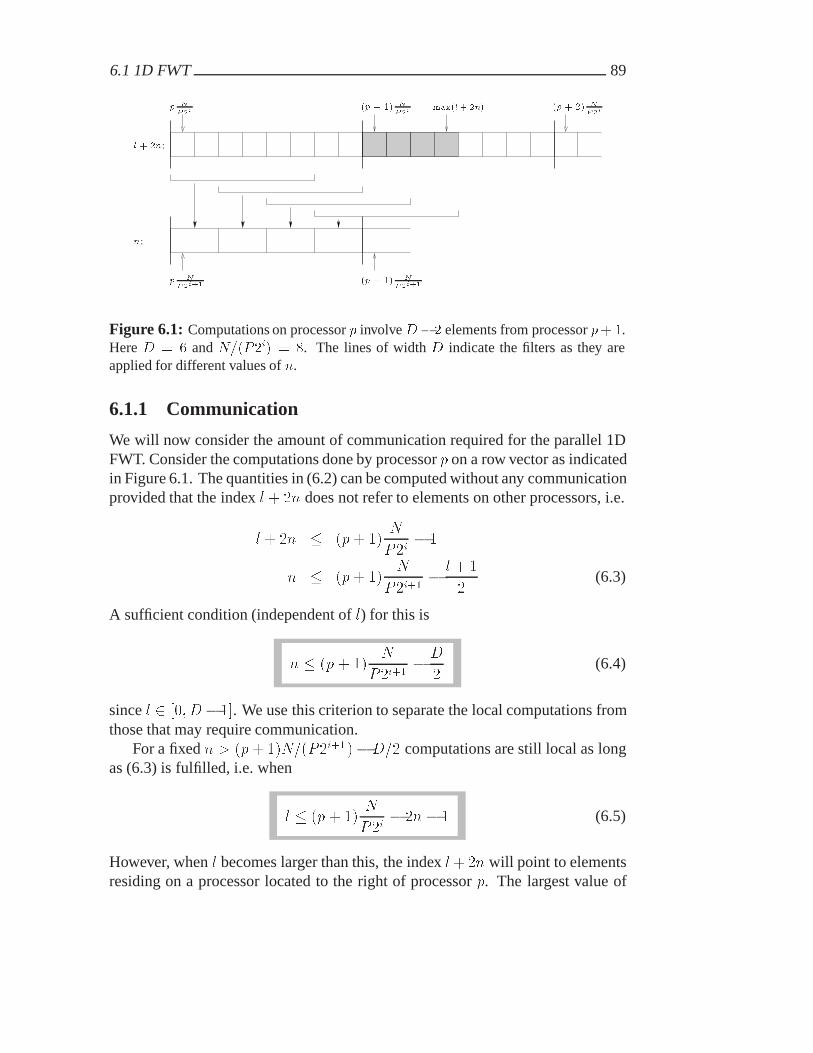
6.1 1D FWT 89
�p � �� N
P�i�p � �� N
P�imax�l � �n�
�p � �� N
P�i��
p N
P�i
p N
P�i��
l � �n:
n:
Figure 6.1: Computations on processor p involve D� � elements from processor p��.Here D � � and N��P�i � �. The lines of width D indicate the filters as they areapplied for different values of n.
6.1.1 Communication
We will now consider the amount of communication required for the parallel 1DFWT. Consider the computations done by processor p on a row vector as indicatedin Figure 6.1. The quantities in (6.2) can be computed without any communicationprovided that the index l � �n does not refer to elements on other processors, i.e.
l� �n � �p� ��N
P�i� �
n � �p� ��N
P�i��� l � �
�(6.3)
A sufficient condition (independent of l) for this is
n � �p � ��N
P�i��� D
�(6.4)
since l � ��D� ��. We use this criterion to separate the local computations fromthose that may require communication.
For a fixed n � �p� ��N��P�i����D�� computations are still local as longas (6.3) is fulfilled, i.e. when
l � �p � ��N
P�i� �n� � (6.5)
However, when l becomes larger than this, the index l��n will point to elementsresiding on a processor located to the right of processor p. The largest value of

90 Parallelization of the Fast Wavelet Transform
l � �n (found from (6.2) and (6.1)) is
max�l � �n� � �p� ��N
P�i�D � � (6.6)
The largest value of l � �n for which communication is not necessary is
�p� ��N
P�i� �
Subtracting this quantity from (6.6) we find that exactly D � � elements must becommunicated to processor p at each step of the FWT as indicated in Figure 6.1.
A tighter bound on �
It is a condition for good performance that the communication pattern describedabove takes place between nearest neighbors only. Therefore, we want to avoidsituations where processor p needs data from processors other than its right neigh-bor hp � �iP so we impose the additional restriction
max�l � �n� � �p � ��N
P�i� �
�p� ��N
P�i�D � � � �p � ��
N
P�i� �
D � � � N
P�i(6.7)
Since we want (6.7) to hold for all i � �� �� � � � � �� � we get
D � � � N
P����
from which we obtain the final bound on �:
� � log�
�N
�D � ��P
(6.8)
For N � ���, D � �, P � ��, for example, we find
� � �
The bound given in (6.8) is not as restrictive as it may seem: Firstly, for the ap-plications where a parallel code is called for, one normally has N � max�P�D�,secondly, in most practical wavelet applications one takes � to be a fixed smallnumber, say �–� [Str96], and thirdly, should the need arise for a large value of�, one could use a sequential code for the last steps of the FWT as these will notinvolve large amounts of data.

6.2 Multiple 1D FWT 91
6.2 Multiple 1D FWT
The considerations from the previous section are still valid if we replace singleelements with columns. This is a parallel version of the MFWT described inSection 5.3. Figure 6.2 shows the data layout of the parallel MFWT algorithm.
accessMemory
FWT direction
� � ��
M
N
Figure 6.2: Multiple FWT. Data are distributed columnwise on the processors. TheFWT is organized rowwise in order to access data with stride one.
The amount of necessary communication is now M�D � �� elements insteadof D � �, the columns of X are distributed blockwise on the processors, and thetransformation of the rows ofX involves the recursion formulas corresponding toXW T
N . The recursion formulas take the same form as in Section 5.3. The onlydifference from the sequential case is that n is now given as in (6.1).
We are now ready to give the algorithm for computing one step of the mul-tiple 1D FWT. The full transform is obtained by repeating this step for i ��� �� � � � � � � �. The algorithm falls naturally into the following three phases:
1. Communication phase: D�� columns are copied from the right neighboras these are sufficient to complete all subsequent computations locally. Wedenote these columns by the block �ci����D��.
2. Fully local phase: The interior of each block is transformed, possibly over-lapping the communication process.
3. Partially remote phase: When the communication has completed, the re-maining elements are computed using �ci��l��n�N��P�i� wheneverl � �n � N��P�i�.

92 Parallelization of the Fast Wavelet Transform
Algorithm 6.1: MFWT, level i� i� �
SPi � N
P�i
p �“my processor id” � � � P � ��
!———————————–! Communication phase!———————————–send ci����D�� to processor hp � �iPreceive �ci����D�� from processor hp � �iP
!————————————–! Fully local phase, cf. (6.4)!————————————–for n � � � SP
i ���D��
ci����n �PD��
l�� alci��l��n ! min�l � �n� � �
di����n �PD��
l�� blci��l��n ! max�l� �n� � SP
i � �end
!———————————————————————–! Partially remote phase! communication must be finished at this point!———————————————————————–for n � SP
i �� �D�� � � � SPi �� � �
!—————————! Local part, cf (6.5)!—————————
ci����n �PSPi ��n��
l�� alci��l��n ! min�l � �n� � SP
i �D � �
di����n �PSPi ��n��
l�� blci��l��n ! max�l� �n� � SP
i � �
!————————————–! Remote part, use �cj����D��!————————————–ci����n �
PD��l�SPi ��n al�c
i��l��n�SPi
! min�l � �n� � SPi
di����n �PD��
l�SPi ��n bl�ci��l��n�SPi
! max�l� �n� � SPi �D � �
end

6.2 Multiple 1D FWT 93
6.2.1 Performance model for the multiple 1D FWT
The purpose of this section is to focus on the impact of the proposed communi-cation scheme on performance with particular regard to speedup and efficiency.We will consider the theoretically best achievable performance of the multiple 1DFWT algorithm. Recall that (5.6) can be computed using
FMFWT�N� � �DMN
� � �
��N
(6.9)
floating point operations. We emphasize the dependency on N because it denotesthe dimension over which the problem is parallelized.
Let tf be the average time it takes to compute one floating point operation ona given computer2. Hence, the time needed to compute (5.6) sequentially is
T �MFWT�N� � FMFWT�N�tf (6.10)
and the theoretical sequential performance becomes
R�MFWT�N� �
FMFWT�N�
T �MFWT�N�
(6.11)
In our proposed algorithm for computing (5.6) the amount of double precisionnumbers that must be communicated between adjacent neighbors at each step ofthe wavelet transform is M�D � �� as described in Section 6.2. Let tl be the timeit takes to initiate the communication (latency) and td the time it takes to sendone double precision number. Since there are � steps in the wavelet transform asimple model for the total communication time is
CMFWT � ��tl �M�D � ��td� (6.12)
Note that CMFWT grows linearly with M but that it is independent of the numberof processors P as well as the size of the second dimension N !
Combining the expression for computation time and communication time weobtain a model describing the total execution time on P processors (P � �) as
T PMFWT�N� �
T �MFWT�N�
P� CMFWT (6.13)
2This model for sequential performance is simplified by disregarding effects arising from theuse of cache memory, pipelining or super scalar processors. Adverse effects resulting from sub-optimal use of these features are assumed to be included in tf to give an average estimate of theactual execution time. Thus, if we estimate tf from the sequential model (6.10), it will normallybe somewhat larger than the nominal value specified for a given computer. In case of the linearmodel for vector performance (5.1) we get for example tf � ts�F � tv.

94 Parallelization of the Fast Wavelet Transform
and the performance of the parallel algorithm is
RPMFWT�N� �
FMFWT�N�
T PMFWT�N�
(6.14)
The expressions for performance in (6.11), (6.14), and (6.13) lead to a formulafor the speedup of the MFWT algorithm:
SPMFWT�N� �
T �MFWT�N�
T PMFWT�N�
�P
� � PCMFWT�T �MFWT�N�
The efficiency of the parallel implementation is defined as the speedup per pro-cessor and we have
EPMFWT�N� �
SPMFWT�N�
P�
�
� � PCMFWT�T �MFWT�N�
(6.15)
It can be seen from (6.15) that for constant N , the efficiency will decrease whenthe number of processors P is increased.
We will now investigate how the above algorithm scales with respect to thenumber of processors when the amount of work per processor is held constant.Thus let N� be the constant size of a problem on one processor. Then the to-tal problem size becomes N � PN� and we find from (6.9) and (6.10) thatT �
MFWT�PN�� � PT �MFWT�N�� because the computational work of the FWT is
linear in N . This means in turn that the efficiency for the scaled problem takes theform
EPMFWT�PN�� �
�
� �PCMFWT
PT �MFWT�N��
��
� � CMFWT�T �MFWT�N��
Since EPMFWT�PN�� is independent of P the scaled efficiency is constant. Hence
the multiple 1D FWT algorithm is fully scalable.

6.3 2D FWT 95
6.3 2D FWT
In this section we will consider two approaches to parallelize the split-transposealgorithm for the 2D FWT as described in Section 5.4.
The first approach is similar to the way 2D FFTs can be parallelized [Heg96]in that it uses the sequential multiple 1D FWT and a parallel transpose algorithm;we denote it the replicated FWT. The second approach makes use of the parallelmultiple 1D FWT described in Section 6.2 to avoid the parallel transposition. Wedenote this approach the communication-efficient FWT.
In both cases we assume that the transform depth is the same in each dimen-sion, i.e. � � �M � �N . Then we get from (3.40) and (5.7) that the sequentialexecution time for the 2D FWT is
T �FWT2�N� � �T �
MFWT�N�� (6.16)
6.3.1 Replicated FWT
The most straightforward way of dividing the work involved in the 2D FWT al-gorithm among a number of processors is to parallelize along the first dimensionin X , such that a sequence of 1D row transforms are executed independently oneach processor. This is illustrated in Figure 6.3. Since we replicate independentrow transforms on the processors we denote this approach the replicated FWT(RFWT) algorithm. Here it is assumed that the matrixX is distributed such that
Memory
FWT direction FWT direction
Transpose
accessMemoryaccess
�
�
�
�M
N
N
M
�
�
�
�
Figure 6.3: Replicated FWT. The shaded block moves from processor � to �.
each processor receives the same number of consecutive rows of X. The first andthe last stages of Algorithm 5.1 are thus done without any communication. How-ever, the intermediate stage, the transposition, causes a substantial communicationoverhead. A further disadvantage of this approach is the fact that it reduces themaximal vector length available for vectorization from M to M�P (and from Nto N�P ). This is a problem for vector architectures such as the Fujitsu VPP300as decribed in section 5.3.

96 Parallelization of the Fast Wavelet Transform
P1
P2
P3
P4
2 3 4
1 3 4
1
1
2
2
4
3
Figure 6.4: Communication of blocks, first block-diagonal shaded.
A similar approach was adopted in [LS95] where a 2D FWT was implementedon the MasPar - a data parallel computer with 2048 processors. It was noted that“the transpose operations dominate the computation time” and a speedup of nomore than � times relative to the best sequential program was achieved.
A suitable parallel transpose algorithm needed for the replicated FWT is onethat moves data in wrapped block diagonals as outlined in the next section.
Parallel transposition and data distribution
Assume that the rows of the matrix X are distributed over the processors, suchthat each processor gets M�P consecutive rows, and that the transpose XT isdistributed such that each processor gets N�P rows. Imagine that the part ofmatrix X that resides on each processor is split columnwise into P blocks, assuggested in Figure 6.4, then the blocks denoted by i are moved to processor iduring the transpose. In total each processor must send P � � blocks and eachblock contains M�P times N�P elements ofX . Hence, following the notation inSection 6.2.1, we get the model for communication time of a parallel transposition
CRFWT � �P � ��
tl �
MN
P �td
(6.17)
Note that CRFWT grows linearly with M , N and P (for P large).
Performance model for the replicated FWT
We are now ready to derive a performance model for the replicated FWT algo-rithm. Using (6.16) and (6.17) we obtain the parallel execution time as
T PRFWT�N� �
T �FWT2�N�
P� CRFWT
and the theoretical speedup for the scaled problem N � PN� is
SPRFWT�PN�� �
P
� � CRFWT�T �FWT2�N��
(6.18)
We will return to this expression in Section 6.3.3.
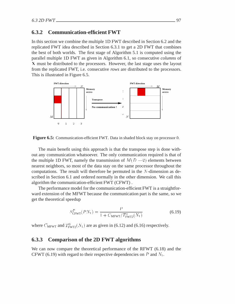
6.3 2D FWT 97
6.3.2 Communication-efficient FWT
In this section we combine the multiple 1D FWT described in Section 6.2 and thereplicated FWT idea described in Section 6.3.1 to get a 2D FWT that combinesthe best of both worlds. The first stage of Algorithm 5.1 is computed using theparallel multiple 1D FWT as given in Algorithm 6.1, so consecutive columns ofX must be distributed to the processors. However, the last stage uses the layoutfrom the replicated FWT, i.e. consecutive rows are distributed to the processors.This is illustrated in Figure 6.5.
No communication !
FWT direction FWT direction
access access
Transpose
Memory Memory
� � ��
M
N
N
M
�
�
�
�
Figure 6.5: Communication-efficient FWT. Data in shaded block stay on processor �.
The main benefit using this approach is that the transpose step is done with-out any communication whatsoever. The only communication required is that ofthe multiple 1D FWT, namely the transmission of M�D � �� elements betweennearest neighbors, so most of the data stay on the same processor throughout thecomputations. The result will therefore be permuted in the N -dimension as de-scribed in Section 6.1 and ordered normally in the other dimension. We call thisalgorithm the communication-efficient FWT (CFWT) .
The performance model for the communication-efficient FWT is a straightfor-ward extension of the MFWT because the communication part is the same, so weget the theoretical speedup
SPCFWT�PN�� �
P
� � CMFWT�T�FWT2�N��
(6.19)
where CMFWT and T �FWT2�N�� are as given in (6.12) and (6.16) respectively.
6.3.3 Comparison of the 2D FWT algorithms
We can now compare the theoretical performance of the RFWT (6.18) and theCFWT (6.19) with regard to their respective dependencies on P and N�.

98 Parallelization of the Fast Wavelet Transform
0 20 40 60 80 100 120 1400
20
40
60
80
100
120
140Scaled speedup
P
SP
Comm−effic.Replicated Perfect
Figure 6.6: The theoretical scaled speedup of the replicated FWT algo-rithm and the communication-efficient FWT shown together with the line ofperfect speedup. The predicted performances correspond to a problem withM � ��� N � ���� D � ��. The characteristic parameters were measuredon an IBM SP2 to be td � ��� �s� tl � ��� �s� tf � � ns. The performance ofthe communication-efficient FWT is much closer to the line of perfect speedup than theperformance of the replicated FWT, and the slope of the curve remains constant.
In case of the CFWT the ratio CMFWT�T�FWT2�N�� is constant with respect to
P whereas the corresponding ratio for the RFWT in (6.18) goes as O�P �:
CRFWT
T �FWT2�N��
� �P � ��tl �P��P � MN�td
�DMN�� O�P �
This means that the efficiency of the RFWT will deteriorate as P grows whileit will stay constant for the CFWT. The corresponding speedups are shown inFigure 6.6.
When P is fixed and the problem size N� grows, then CMFWT�T�FWT2�N�� goes
to zero, which means that the scaled efficiency of the CFWT will approach theideal value �. For the RFWT the corresponding ratio approaches a positive con-stant as N� grows:
CRFWT
T �FWT2�N��
� �P � ��td�DP �
for N� ��

6.3 2D FWT 99
P N Mflop/s Efficiency (%) Estim. eff.� ��� ��� ��� ��� ����� ������ � � �� ����� ������ �� ��� ����� ������ ���� ���� ����� �����
�� ���� ���� ����� ������ ���� ���� ����� �����
Table 6.3: Communication-efficient FWT on the SP2. N � PN�, N� � ���,M � ���,D � ��. P � � signifies sequential performance. Estimated efficience is given asSPCFWT�PN��P where SPCFWT�PN� is given as in (6.19).
This means that the scaled efficiency of the RFWT is bounded by a constant lessthan one – no matter how large the problem size. The asymptotic scaled efficien-cies of the two algorithms are summarized below
P �� N� ��
Replicated FWT:�
� �O�P �
�
� � �P���td�DP �
Communication-efficient FWT:
�
� �CMFWT
T �FWT2�N��
�
6.3.4 Numerical experiments
We have implemented the communication-efficient FWT on two different MIMDcomputer architectures, namely the IBM SP2 and the Fujitsu VPP300. On the SP2we used MPI for the parallelism whereas the proprietary VPP Fortran was usedon the VPP300.
The IBM SP2 is a parallel computer which is different from the VPP300. Eachnode on the SP2 is essentially a workstation which does not achieve the perfor-mance of a vector processor such as the VPP300. High performance on the SP2must therefore be achieved through a higher degree of parallelism than on theVPP300 and scalability to a high number of processors is more urgent in thiscase. The measured performances on the IBM SP2 are shown in Table 6.3.

100 Parallelization of the Fast Wavelet Transform
0 5 10 15 20 25 30 350
5
10
15
20
25
30
35Scaled speedup
P
SP
TheoreticalMeasured Ideal
Figure 6.7: Scaled speedup, communication-efficient FWT (IBM SP2). These graphsdepict how the theoretical performance model does, in fact, give a realistic prediction ofthe actual performance.
P N Mflop/s Efficiency (%)� �� ���� �� ���� ����� ���� � � ������ ���� � � ������ ���� ����� �����
Table 6.4: Communication-efficient FWT on the VPP300. N � P , M � ��, D � ��.P � � signifies sequential performance.
It is seen that the performance scales well with the number of processors and,furthermore, that it agrees with the predicted speedup as shown in Figure 6.7. Theparallel performance on the Fujitsu VP300 is shown in Table 6.4. We have not es-timated the characteristic numbers tl� td� tf for this machine, but it is neverthelessclear that the performance scales almost perfectly with the number of processorsalso in this case.

6.4 Summary 101
6.4 Summary
We have developed a new parallel algorithm for computing the 2D wavelet trans-form, the communication-efficient FWT.
Our new approach avoids the use of a distributed matrix transpose and per-forms significantly better than algorithms that require such a transpose. This isdue to the fact that the communication volume of a parallel transpose is largerthan necessary for computing the 2D FWT.
The communication-efficient FWT is optimal in the sense thatthe scaled efficiency is independent of the number of proces-sors and that it approaches � as the problem size is increased.
Implementations on the Fujitsu VPP300 and the IBM SP2 confirms the scalabilityof the CFWT algorithm.

Part III
Wavelets and Partial DifferentialEquations

Chapter 7
Wavelets and differentiationmatrices
7.1 Previous wavelet applications to PDEs
Even though the field of wavelet theory has had a great impact on other fields,such as signal processing, it is not yet clear whether it will have a similar impacton numerical methods for solving partial differential equations (PDEs).
In the early nineties people were very optimistic because it seemed that thenice properties of wavelets would automatically lead to efficient solution meth-ods for PDEs. The reason for this optimism was the fact that many nonlinearPDEs have solutions containing local phenomena (e.g. formation of shocks) andinteractions between several scales (e.g. turbulence). Such solutions can oftenbe well represented in wavelet bases, as explained in the previous chapters. Itwas therefore believed that efficient wavelet-based numerical schemes for solvingthese PDEs would follow from wavelet compression properties [BMP90, LT90b,LPT92, HPW94, GL94, CP96, PW96, F�96, DKU96].
However, this early optimism remains to be honored. Wavelets have not hadthe expected impact on differential equations, partly because the computationalwork is not necessarily reduced by applying wavelet compression - even thoughthe solution is sparsely represented in a wavelet basis. In the following chapterswe will discuss some of the most promising approaches and shed some light onthe obstacles that must be overcome in order to obtain successful wavelet-basedPDE solvers.
Schematically, wavelet-based methods for PDEs can be separated into the fol-lowing classes:

106 Wavelets and differentiation matrices
Class 1: Methods based on scaling function expansions
The unknown solution is expanded in scaling functions at some chosen level Jand is solved using a Galerkin approach. Because of their compact support, thescaling functions can be regarded as alternatives to splines or the piecewise poly-nomials used in finite element schemes. While this approach is important in itsown right, it cannot exploit wavelet compression. Hence methods in this categoryare not adaptive [LT90a, QW93, WA94, LR94, Jam93, RE97]. However, this ap-proach has many points of interest. Leland Jameson [Jam93] has shown that oneobtains a method which exhibits super convergence at the grid points, the order ofapproximation being twice as large as that of the projection of the solution ontothe space spanned by scaling functions. Johan Walden [Wal96] has shown thatthe size of the differentiation filters grows faster than the optimal centered finitedifference method of the same order. In the limit, as the order goes to infinity, itis shown that
R���x � k���x� dx � ����k�k for D � �. Finally, we mention
that Teresa Reginska and others [RE97, EBR97] use scaling functions to regular-ize the solution of the sideways heat equation. This is an ill-posed problem in thesense that the solution does not depend continuously on the initial condition. Byexpanding the solution in scaling functions, high frequency components can befiltered away and continuous dependence of the initial condition is restored.
Class 2: Methods based on wavelet expansions
The PDE is solved using a Galerkin approach as in the first class. In this case,however, the unknown solution is expressed in terms of wavelets instead of scalingfunctions so wavelet compression can be applied; either to the solution [LT90b],the differential operator [BCR91, Bey92, EOZ94, XS92], or both [CP96, BK97,PW96]. Several different approaches have been considered for exploiting the spar-sity of a wavelet representation. One is to perform all operations in the waveletdomain [BN96, BMP90, Wal96]. The operators are sparse but the number of sig-nificant coefficients in the solutions Ns��� has to be very small compared to thedimension of the problemN for the methods to be efficient. This is especially truefor non-linear operations. However, recent work by Beylkin and Keiser [BK97]suggests that some nonlinearities may be efficiently treated in the wavelet domain.
In another approach linear operations such as differentiation are done in thewavelet domain and nonlinear operations such as squaring in the physical domain.This is by far the most common approach and it is used by [Kei95, CP96, FS97,PW96, EOZ94, VP96] and the author. This approach involves a number of trans-formations between the physical domain and the wavelet domain in each timestep, and this can introduce considerable overhead. Hence, the wavelet compres-sion potential of the solution must be very large for this approach to be feasible.

7.1 Previous wavelet applications to PDEs 107
An interesting aspect of the wavelet approach is that certain operators repre-sented with respect to a wavelet basis become sparser when raised to higher pow-ers [EOZ94]. From this property one can obtain an efficient time-stepping schemefor certain evolution equations. This method has been employed in [CP96, Dor95]to solve the heat equation.
Finally, we mention that several papers have exploited the so-called Non-standard or BCR form of the differential operator [BCR91, Bey92, Dor95, BK97].This form is sparser than the standard form, but to apply the non-standard form ofthe differential operator to a function one needs to know, at all scales, the scalingfunction coefficients of the function as well as its wavelet coefficients. This repre-sentation is redundant and, even though the function may be sparse in its waveletrepresentation, the scaling function representation may not be sparse.
We will refer to methods from Class � and � as projection methods.
Class 3: Wavelets and finite differences
In the third approach wavelets are used to derive adaptive finite difference meth-ods. Instead of expanding the solution in terms of wavelets, the wavelet transformis used to determine where the finite difference grid must be refined or coarsenedto optimally represent the solution. The computational overhead is low becauseone works with point values in the physical representation. One approach was de-veloped by Leland Jameson, [Jam94, Jam96] under the name Wavelet OptimizedFinite Difference Method (WOFD). Walden describes a filter bank method in[Wal96], Matts Holmstrom has introduced the Sparse Point Representation (SPR)in [Hol97], and also [PK91] have used wavelets to localize where to apply gridrefinement.
Class 4: Other methods
There are a few approaches that use wavelets in ways that do not fit into any of theprevious classes. Examples are operator wavelets [JS93, EL], anti-derivatives ofwavelets [XS92], the method of travelling wavelets [PB91, WZ94], and wavelet-preconditioning [Bey94].
Operator wavelets are wavelets that are (bi-)orthogonal with respect to an in-ner product designed for the particular differential operator in question. This isnot a general method since it works only for certain operators. The use of anti-derivatives of wavelets is similar to that of operator wavelets.
In the method of travelling wavelets, an initial condition is expanded usingonly a few wavelets which are then propagated in time. A disadvantage of this

108 Wavelets and differentiation matrices
method is that these few wavelets may be unable to express the solution after ithas been propagated for a time.
Finally, in [Bey94] it is shown that any finite difference matrix representa-tion of periodized differential operators can be preconditioned so that the condi-tion number is O���. Furthermore, if the difference matrix is represented in awavelet basis (the standard form) then the preconditioner is a diagonal matrix.Thus, wavelets play an auxiliary role in that they provide a means to reduce thecondition number of the operator.
In this chapter and Chapter 8 we describe the necessary background for methodsbelonging to Class � and �. In Chapter 9 we give some applications of thesemethods to PDEs, and we also illustrate the WOFD method from Class �. We willnot discuss further methods belonging to class 4.
7.2 Connection coefficients
A natural starting point for the projection methods is the topic of two-term con-nection coefficients. The description adopted here is similar to the one describedin [LRT91] and [Bar96]. An alternative method is described in [Kun94]. Wedefine the connection coefficients as
d��d�j�l�m �
Z �
����d��j�l �x��
�d��j�m �x� dx� j� l�m � Z
where d� and d� are orders of differentiation. We will assume for now that thesederivatives are well-defined.
Using the change of variable x� ��jx� l� one obtains
d��d�j�l�m � �jdZ �
����d���x���d���x�m� l� dx � �jd d��d�����m�l
where d � d� � d�. Repeated integration by parts yields the identity d� �d�����n �
����d� ��d����n because the scaling functions have compact support. Hence
d��d�j�l�m � ����d��jd ��d����m�l
Therefore it is sufficient to consider only one order of differentiation �d� and oneshift parameter �m� l� and we define
dl �
Z �
����x��
�d�l �x� dx� l � Z (7.1)

7.2 Connection coefficients 109
Consequently
d��d�j�l�m � ����d��jd dm�l (7.2)
and we note the property
dn � ����d d�n� n � ��D�D � �� (7.3)
which is obtained using the change of variable x � x � l in (7.1) followed byrepeated integration by parts.
In the following we will restrict our attention to the problem of computing(7.1). The supports of � and ��d�l overlap only for��D� �� � l � D� � so thereare �D � � nonzero connection coefficients to be determined. Let
�d � f dl gD��l���D
and assume that � � Cd�R�. Then taking the identity (3.21) with j � � anddifferentiating it d times leads to
��d�l �x� �
D��Xk��
ak��d����l�k�x� � �d
p�D��Xk��
ak��d��l�k��x� (7.4)
Substituting the dilation equation (2.17) and (7.4) into (7.1) yields
dl �
Z �
��
(p�
D��Xr��
ar�r��x�
)(�dp�
D��Xs��
as��d��l�s��x�
)dx
� �d��D��Xr��
D��Xs��
aras
Z �
���r��x��
�d��l�s��x� dx� x� �x
� �dD��Xr��
D��Xs��
aras
Z �
���r�x��
�d��l�s�x� dx� x� x� r
� �dD��Xr��
D��Xs��
aras
Z �
����x���d��l�s�r�x� dx
or
D��Xr��
D��Xs��
aras d�l�s�r �
�
�d dl � l � ��D�D � �� (7.5)

110 Wavelets and differentiation matrices
Let n � �l� s� r. We know that dn is nonzero only for n � ��D�D � �� andthat s � r � n � �l as well as r must be restricted to ��D � ��. This is fulfilledfor max��� �l�n� � r � min�D� ��D� ���l�n�. Let p � �l�n and define
ap �
r��p�Xr�r��p�
arar�p
where r��p� � max��� p� and r��p� � min�D � ��D � � � p� . Hence (7.5)becomes
D��Xn���D
a�l�n dn ��
�d dl � l � ��D�D � ��
The matrix-vector form of this relation is�A� ��dI
��d � � (7.6)
where A is a ��D � ��� ��D � �� matrix with the elements
A�l�n � a�l�n� l� n � ��D�D � ��
We note the following properties of a:
� Because of the orthogonality property (2.22) we have
ap �
�� for p � �� for p � �������� � � �
� Also, ap � a�p so we need only compute ap for p � �.
� Finally, a consequence of Theorem 2.3 is thatXp odd
ap � �
Hence all columns add to one, which means that A has the left eigenvector�� �� � � � � �� corresponding to the eigenvalue �, d � � in (7.6).
Consequently, A has the structure shown here for D � �:��������������
� a�� a� � a�� a� � a� � a�� a� � a� � a� � a�� a� � a� � a� � a� �
a� � a� � a� � a� �a� � a� � a� �
a� � a� �a� �
��������������

7.2 Connection coefficients 111
Equation (7.6) has a non-trivial solution if ��d is an eigenvalue of A. Nu-merical calculations for D � �� �� � � � � �� indicate that ��d is an eigenvalue ford � �� �� � � � �D � � and that the dimension of each corresponding eigenspace is�. Hence one additional equation is needed to normalize the solution.
To this end we use the property of vanishing moments. Recall that P � D��.Assuming that d � P we have from (2.25) that
xd ��X
l���Md
l ��x� l�
Differentiating both sides of this relation d times yields
d� ��X
l���Md
l ��d��x� l�
Multiplying by ��x� and integrating we then obtain
d�
Z �
����x� dx �
�Xl���
Mdl
Z �
����x���d��x� l� dx
�D��X
l���DMd
l
Z �
����x���d��x� l� dx
Hence we get
D��Xl���D
Mdl
dl � d� (7.7)
which closes the the system (7.6). The computation of the moments needed forthis equation is described in Appendix (A). �d is then found as follows: Let vd bean eigenvector corresponding to the eigenvalue ��d in (7.6). Then �d � kvd forsome constant k, which is fixed according to (7.7).
The Matlab function conn(d,D) computes �d for a given wavelet genus D.
Remark 7.1 There is one exception to the statement that ��d is an eigenvalue ofA for d � �� �� � � � �D � �: Let D � �. Then the eigenvalues ofA are
�
��
�
�� ������ � ����i�
�
�� ������ � ����i�
�
�� �
Consequently �� is not an eigenvalue ofA and connection coefficients for the com-
bination D � �� d � � are not well defined.
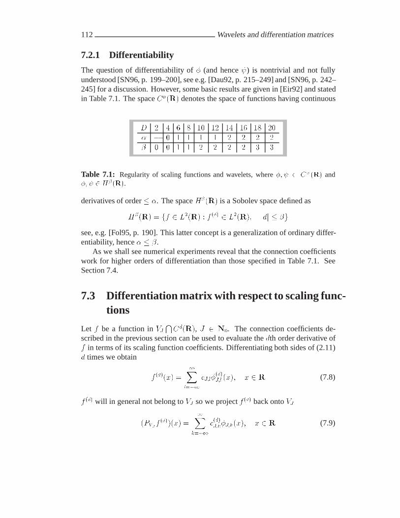
112 Wavelets and differentiation matrices
7.2.1 Differentiability
The question of differentiability of � (and hence �) is nontrivial and not fullyunderstood [SN96, p. 199–200], see e.g. [Dau92, p. 215–249] and [SN96, p. 242–245] for a discussion. However, some basic results are given in [Eir92] and statedin Table 7.1. The space C�R� denotes the space of functions having continuous
D � � � � �� �� �� �� �� ��� � � � � � � � � � �� � � � � � � � � � �
Table 7.1: Regularity of scaling functions and wavelets, where �� � � C�R and�� � � H��R.
derivatives of order � �. The space H��R� is a Sobolev space defined as
H��R� � ff � L��R� � f �d� � L��R�� jdj � �gsee, e.g. [Fol95, p. 190]. This latter concept is a generalization of ordinary differ-entiability, hence � � �.
As we shall see numerical experiments reveal that the connection coefficientswork for higher orders of differentiation than those specified in Table 7.1. SeeSection 7.4.
7.3 Differentiation matrix with respect to scaling func-tions
Let f be a function in VJTCd�R�, J � N�. The connection coefficients de-
scribed in the previous section can be used to evaluate the dth order derivative off in terms of its scaling function coefficients. Differentiating both sides of (2.11)d times we obtain
f �d��x� �
�Xl���
cJ�l��d�J�l �x�� x � R (7.8)
f �d� will in general not belong to VJ so we project f �d� back onto VJ
�PVJf�d���x� �
�Xk���
c�d�J�k�J�k�x�� x � R (7.9)

7.3 Differentiation matrix with respect to scaling functions 113
where, according to (2.12),
c�d�J�k �
Z �
��f �d��x��J�k�x� dx (7.10)
Substituting (7.8) into (7.10) we find
c�d�J�k �
�Xl���
cJ�l
Z �
���J�k�x��
�d�J�l �x� dx
��X
l���cJ�l
��dJ�k�l
��X
l���cJ�l�
Jd dl�k
��X
n���cJ�n�k �
Jd dn� �� � k ��
We used (7.2) for the second last equality. Since dn is only nonzero for n ���D�D � �� we find that
c�d�J�k �
D��Xn���D
cJ�n�k�Jd dn� J� k � Z (7.11)
Recall from (2.60) that if f is �-periodic then
cJ�l � cJ�l�p�J � l� p � Z
and
c�d�J�k � c
�d�
J�k�p�J� k� p � Z
Hence, it is sufficient to consider �J coefficients of either type and (7.11) becomes
c�d�J�k �
D��Xn���D
cJ�hn�ki�J �Jd dn� k � �� �� � � � � �J � � (7.12)
This system of equations can be represented in matrix-vector form
c�d� �D�d�c (7.13)

114 Wavelets and differentiation matrices
where
D�d��k�hn�ki�J � �Jd dn� k � �� �� � � � � �J � ��
n � ��D� � �D� � � � �D � �
and c�d� � c�d�J��� c
�d�J��� � � � � c
�d�
J��J���.
We will refer to the matrix D�d� as the differentiation matrix of order d. Itcan be seen from (7.3) that D�d� is symmetric for d even and skew-symmetric ford odd. Furthermore, it follows that D�d� is circulant as defined in Definition C.1and that it has bandwidth �D � �. The differentiation matrix has the followingstructure (shown for D � � and J � �):
D�d� � ��
������������
�d� �d� �d� � � � ����d�d� ����d�d�����d�d� �d� �d� �d� � � � ����d�d�����d�d� ����d�d� �d� �d� �d� � � �
� ����d�d� ����d�d� �d� �d� �d� � �
� � ����d�d� ����d�d� �d� �d� �d� �
� � � ����d�d� ����d�d� �d� �d� �d�
�d� � � � ����d�d� ����d�d� �d� �d�
�d� �d� � � � ����d�d� ����d�d� �d�
������������
An important special case is d � �, and we define
D �D��� (7.14)
7.4 Differentiation matrix with respect to physicalspace
We will restrict our attention to the periodic case. Recall from Section 3.2.3 that
f � Tc� c � T��f
where f are the grid values of a function f � �VJ defined on the unit interval. c isthe vector of scaling function coefficients corresponding to f , and T is the matrixdefined in (3.16) which maps from the scaling function coefficients onto the gridvalues. Similarly, the projection of f �d� onto �VJ satisfies
f �d� � Tc�d�

7.4 Differentiation matrix with respect to physical space 115
Then it follows from (7.13) that
f �d� � TD�d�T��f
We callD�d� the differentiation matrix with respect to the coefficient space, byvirtue of (7.13), and TD�d�T�� the differentiation matrix with respect to physicalspace. The matrices T and D�d� are both circulant with the same dimensions��D � �� � ��D � ��, so they are diagonalized by the same matrix, namely theFourier matrix F �D�� defined in (C.3). Therefore, they commute, according toTheorem C.5, and we find that
TD�d�T�� �D�d�TT�� �D�d�
and
f �d� �D�d�f (7.15)
HenceD�d� is the differentiation matrix with respect to both coefficient space andphysical space.
If f is an arbitrary 1-periodic function then f �d� will generally not be exactdue to approximation errors and we define
E�d��f� J� � maxk����� ��J��
����hf �d�ik� f �d�
k
�J
����Jameson [Jam93] establishes the following convergence result for the differentia-tion matrix D���:
f � CD�R� � E����f� J� � C��JD (7.16)
where C is a constant. Assume that similar results hold for higher orders of dif-ferentiation, i.e.
E�d��f� J� � C��JR� R � R� d � � (7.17)
where R possibly depends on d and D. Taking the logarithm on both sides of(7.17) yields
log��E�d��f� J�� � log��C��JR� � log��C�� JR
and we can find the convergence rate R from the differences
log��E�d��f� J��� log��E
�d��f� J � ��� � R

116 Wavelets and differentiation matrices
Dnd � � � � � � � � � �� �� ��� � � � � � � � � � � � �� � � � � � � � � � � � �� � � � � � � � � � � � ��� �� � � � � � � � � � � ��� �� �� �� � � � � � � � � �
Table 7.2: Convergence rates R (rounded) for the differentiation matrix shown fordifferent values of D and orders of differentiation d. Here, f�x � sin��x, andJ � � �� � � � � �. Note that the case D � �� d � � is not valid as mentioned in Re-mark 7.1.
Numerical results are summarized in Table 7.2 and it is verified that (7.16) applies.For higher orders of differentiation, there is still convergence, but with lower con-vergence rates. We observe that R appears to be given by
R � D � � bd��c � d � �� �� � � � �D � �
Moreover, we observe that numerical differentiation is successfully carried out tomuch higher orders than those suggested in Table 7.1.
The convergence rate R � D for d � � can be achieved also for higher ordersby redefining the differentiation process for d � �. Let
f�d�
�Ddf
i.e. the dth derivative of f is approximated by repeated application of the firstorder differentiation matrix. Define
E�d��f� J� � max
k����� ��J��
����hf �d�ik� f �d�
k
�J
����Then
E�d��f� J� � C��JR� R � R
with R � D. This is confirmed in Table 7.3.Let B�Dd� denote the bandwidth of Dd. We know from (7.13) that B�D� �
�D � �, and the general formula turns out to be:
B�Dd� � min�dB�D�� d � �� �J �
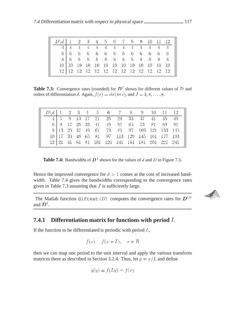
7.4 Differentiation matrix with respect to physical space 117
Dnd � � � � � � � � � �� �� ��� � � � � � � � � � � � �� � � � � � � � � � � � �� � � � � � � � � � � � ��� �� �� �� �� �� �� �� �� �� �� �� ���� �� �� �� �� �� �� �� �� �� �� �� ��
Table 7.3: Convergence rates (rounded) for Dd shown for different values of D andorders of differentiation d. Again, f�x � sin��x, and J � � �� � � � � �.
Dnd � � � � � � � � � �� �� ��� � � �� �� �� �� �� �� �� �� �� ��� � �� �� �� �� �� �� �� �� �� �� ��� �� �� �� �� �� �� �� �� ��� ��� ��� ����� �� �� �� �� �� �� ��� ��� ��� ��� ��� ����� �� �� �� �� ��� ��� ��� ��� ��� ��� ��� ���
Table 7.4: Bandwidths ofDd shown for the values of d and D in Figure 7.3.
Hence the improved convergence for d � � comes at the cost of increased band-width. Table 7.4 gives the bandwidths corresponding to the convergence ratesgiven in Table 7.3 assuming that J is sufficiently large.
The Matlab function diftest(D) computes the convergence rates for D�d�
and Dd.
7.4.1 Differentiation matrix for functions with period L
If the function to be differentiated is periodic with period L,
f�x� � f�x� L�� x � R
then we can map one period to the unit interval and apply the various transformmatrices there as described in Section 3.2.4. Thus, let y � x�L and define
g�y� f�Ly� � f�x�

118 Wavelets and differentiation matrices
Then g is �-periodic and we define the vector g � g�� g�� � � � � g�J��� by
gk � �PVJg��k��J �� k � �� �� � � � � �J � �
Let f � g. Then f approximates f�x� at x � k L��J . From (7.15) we have
g�d� �D�d�g
Hence, by the chain rule
f �d��x� ��
Ldg�d��y�
we have
f �d� ��
Ldg�d� �
�
LdD�d�g �
�
LdD�d�f (7.18)
The Matlab function difmatrix(d,N,L,D) computes the differentiationmatrixD�d��Ld for wavelet genus D and size N and period L.
7.5 Differentiation matrix with respect to wavelets
We will restrict our attention to the periodic case. Let f be a function in �VJ .Proceeding as in the previous section, we differentiate both sides of (2.53) d timesand obtain
f �d��x� ��J���Xl��
cJ��l���d�J��l
�x� �J��Xj�J�
�j��Xl��
dj�l ���d�j�l �x� (7.19)
Projecting f �d� onto �VJ yields
�PVJf�d���x� �
�J���Xl��
c�d�J� �l
��J� �l�x� �J��Xj�J�
�j��Xl��
d�d�j�l
��j�l�x�
where
c�d�J��l
�
Z �
��f �d��x���J��l�x� dx� l � �� �� � � � � �J� � �
d�d�j�l �
Z �
��f �d��x� ��j�l�x� dx� j � J�� J� � �� � � � � J � �
l � �� �� � � � � �j � �
(7.20)

7.5 Differentiation matrix with respect to wavelets 119
Recall that given the scaling function coefficients of f�d� on the finest level, theFWT (3.33) can be used to obtain the wavelet coefficients above. Hence
d�d� �Wc�d�
where c�d� is defined as in Section 7.3 and d�d� contains the coefficients in (7.20).Using (7.13) and (3.35) we then obtain
d�d� �WD�d�c �WD�d�W Td
or
d�d� � �D�d�d (7.21)
where we have defined
�D�d�
�WD�d�W T (7.22)
�D�d�
is the differentiation matrix with respect to the wavelet coefficients. We
observe that �D�d�
is obtained as a 2D FWT of the differentiation matrix D�d�.In contrast to D�d�, the matrix �D
�d�is not circulant. Instead, it has a charac-
teristic finger band pattern as illustrated in Figure (7.1). As will be described in
Chapter 8, one can take advantage of this structure to compute �D�d�
efficiently.

120 Wavelets and differentiation matrices
8 16 32 64
8
16
32
64
nz = 1360
V3
~W
3
~W
4
~W
5
~
V3
~
W3
~
W4
~
W5
~
Figure 7.1: Sparsity pattern of �D�d�
when D � �, L � �, J � �, � � , d � �. Thepattern is identical for d �.

Chapter 8
2D Fast Wavelet Transform of acirculant matrix
In this chapter we will describe an algorithm for computing the 2D fast wavelettransform (2D FWT) of a circulant N �N matrix A. The 2D FWT is defined in(3.38) and circulant matrices are discussed in Appendix C.
Recall that the 2D FWT is a mapping A�H given as
H �WAW T
whereW is defined as in (3.34). We will show that this can be done inO�N� stepsand that H can be represented using O�N� elements in a suitable data structure.Using this structure we describe an efficient algorithm for computing the matrix-vector product
Hx
where x is an arbitrary vector of length N . This algorithm also has complex-ity O�N� and will be used in Chapter 9 in a wavelet method for solving PDEsdeveloped in 9.3.1.
This chapter is based on [Nie97] and the approach follows ideas proposed byPhilippe Charton [Cha96]. However, many of the details, the data structure andthe complexity analysis are, to our knowledge, presented here for the first time.
8.1 The wavelet transform revisited
Let N and � be integers of the form given in Definition 3.1 and let ci be a givenvector with elements ci�� c
i�� � � � � c
iN��� and let di be defined similarly.

122 2D Fast Wavelet Transform of a circulant matrix
Recall that the 1D FWT is defined (and computed) by the recurrence formulasfrom Definition 3.1:
ci��m �D��Xk��
akcihk��miSi
di��m �
D��Xk��
bkcihk��miSi
for i � �� �� � � � � � � �, m � �� �� � � � � Si�� � �, and Si � N��i. Figure 8.1illustrates how a vector is transformed.
c�
d�
c�
d�
d�
c�
d�
d�
d�
c�
� � �
Figure 8.1: The steps of a 1D wavelet transform for � � and J � �.
The 2D FWT defined in (3.38) has also a recursive formulation. The 2D recur-rence formulas are straightforward generalizations of the 1D formulas, and theydecompose a matrix analogously to the way the 1D recurrence formulas decom-pose a vector.
The recursion is initialized by assigning a matrix (assumed to be square forsimplicity) A � RN�N to the initial block1 which we denote CC���. This blockis then successively split into smaller blocks denoted CCi�j , DCi�j , CDi�j , andDDi�j for i� j � �� �� � � � � �. The block dimensions are determined by the super-scripts i� j: A block with indices i� j has Si � N��i rows and Sj � N��j columns.
1We point out that, throughout this chapter, we use two-character symbols for certain matricesand block-matrices.

8.1 The wavelet transform revisited 123
The steps of the 2D wavelet transform for � � � are shown in Figure 8.2 with Hbeing the aggregation of all blocks after the final step shown in the upper rightcorner in the figure. (Comparison with the 1D wavelet transform shown in Fig-ure 8.1 can be helpful for understanding this scheme). Note that each step of thetransform produces blocks that have attained their final values, namely those ofthe type DDi�j , and subsequent steps work on blocks of the type CCj�j , CDi�j ,and DCi�j . The formulas for these three types of blocks are given below.
CC��
�
�
�
CC��
CD��
DC��
DD��
DD��
DD��
DD��
CC��
DC��
CD��
CD��
DD��
DD��
DC��
DD��
DD��
DD��
DD��
CC��
DC��
CD��
DC��
DC��
DD��
DD��
DD��
DD��
CD��
CD��
A H
Figure 8.2: The steps of a 2D wavelet transform for � � and J � �. The resultingmatrixH has the characteristic “arrow-shaped” block structure.
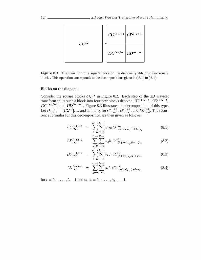
124 2D Fast Wavelet Transform of a circulant matrix
CCi�i �
CCi���i��
DCi���i��
CDi���i��
DDi���i��
Figure 8.3: The transform of a square block on the diagonal yields four new squareblocks. This operation corresponds to the decompositions given in ( 8.1) to ( 8.4).
Blocks on the diagonal
Consider the square blocks CCi�i in Figure 8.2. Each step of the 2D wavelettransform splits such a block into four new blocks denotedCCi���i��, CDi���i��,DCi���i��, and DDi���i��. Figure 8.3 illustrates the decomposition of this type.Let CCi�j
m�n � CCi�j�m�n and similarly for CDi��m�n, DCi��
m�n, and DDi��m�n. The recur-
rence formulas for this decomposition are then given as follows:
CCi���i��m�n �
D��Xk��
D��Xl��
akalCCi�ihk��miSi �hl��niSi
(8.1)
CDi���i��m�n �
D��Xk��
D��Xl��
akblCCi�ihk��miSi �hl��niSi
(8.2)
DC i���i��m�n �
D��Xk��
D��Xl��
bkalCCi�ihk��miSi �hl��niSi
(8.3)
DDi���i��m�n �
D��Xk��
D��Xl��
bkblCCi�ihk��miSi �hl��niSi
(8.4)
for i � �� �� � � � � �� � and m�n � �� �� � � � � Si�� � �.

8.1 The wavelet transform revisited 125
DCi�j � DC i�j�� DDi�j��
Figure 8.4: Transform of a block below the diagonal yields two new rectangular blocks.This operation corresponds to the row transforms given in ( 8.5) and ( 8.6).
Blocks below the diagonal
Blocks of the type DCi�j (j � i) are split in one direction only as indicated inFigure 8.4. The recurrence formulas are the 1D formulas applied to each row ofthe block DCi�j:
DC i�j��m�n �
D��Xl��
alDCi�jm�hl��niSj
(8.5)
DDi�j��m�n �
D��Xl��
blDCi�jm�hl��niSj
(8.6)
for j � i� i� �� � � � � �� �, m � �� �� � � � � Si � �, and n � �� �� � � � � Sj�� � �.

126 2D Fast Wavelet Transform of a circulant matrix
CDi�j �
CDi���j
DDi���j
Figure 8.5: Transform of a block above the diagonal yields two new rectangular blocks.This operation corresponds to the column transforms given in ( 8.7) and ( 8.8).
Blocks above the diagonal
For blocks CDi�j with i � j we have a splitting as shown in Figure 8.5. Therecurrence formulas are the 1D formulas applied to each column of CDi�j:
CDi���jm�n �
D��Xk��
ak CDi�jhk��miSi �n
(8.7)
DDi���jm�n �
D��Xk��
bk CDi�jhk��miSi �n
(8.8)
for i � j� j � �� � � � � �� �, m � �� �� � � � � Si�� � �, and n � �� �� � � � � Sj � �.

8.2 2D wavelet transform of a circulant matrix 127
8.2 2D wavelet transform of a circulant matrix
The 2D FWT of circulant matrices give rise to structured matrix blocks which wewill call shift-circulant matrices. We begin by giving the definition.
Let A be an M � M circulant matrix as defined in Definition C.1 and letfamgm����� �M�� be the first column of A. Then
A�m�n � ahm�niM � m� n � �� �� � � � �M � �
A shift-circulant matrix is a generalization of a circulant matrix which we defineas follows
Definition 8.1 (Shift-circulant matrix)
1. Let A be an M � N matrix where M � N with M divisible by N , andlet famgm����� �M�� be the first column of A. Then A is column-shift-circulant if
A�m�n � ahm��niM � m � �� �� � � � �M � �� n � �� �� � � � � N � �
where � � M�N .
2. Let A be an M �N matrix where N � M with N divisible by M , and letfangn����� �N�� be the first row ofA. ThenA is row-shift-circulant if
A�m�n � ahn��miN � m � �� �� � � � �M � �� n � �� �� � � � � N � �
where � � N�M .
The number � is a positive integer that denotes the amount by which columns orrows are shifted.
A column-shift-circulant �� � matrix (� � �) has the form"BB#
a� a�a� a�a� a�a� a�
$CCA
A row-shift-circulant �� � matrix (� � �) has the forma� a� a� a�a� a� a� a�
Note that a circulant matrix is both column-shift-circulant and row-shift-circulantwith � � �.

128 2D Fast Wavelet Transform of a circulant matrix
Let fangn����� �N�� be the first column of a circulant matrix A. Using thiscolumn vector as a point of departure we will now show how to compute a rep-resentation of H using only one vector per block. Note that according to therecurrence equations (8.1) to (8.8), the operations can be divided into 2D trans-forms of blocks on the diagonal and 1D row or column transforms of off-diagonalblocks. We will treat these cases separately.
8.2.1 Blocks on the diagonal
Lemma 8.1 LetCCi�i be a Si�Si circulant matrix. ThenCCi���i��, CDi���i��,DCi���i��, and DDi���j�� defined by (8.1) to (8.4), respectively, are circulantmatrices.
Proof: We will prove the lemma for CDi���i�� only since the other cases arecompletely analogous.
By assumption CCi�i is circulant, i.e.
CC i�im�n � cci�ihm�niSi
where cci�i is the first column of CCi�i. Equation (8.2) then becomes
CDi���i��m�n �
D��Xk��
D��Xl��
akbl cci�ihhk��miSi�hl��niSiiSi
(8.9)
Considering now the index of the typical term of (8.9) and using Lemma B.1and B.2 derived in Appendix B we find that
hhk � �miSi � hl � �niSiiSi � hh��m � n�iSi � k � liSi� h�hm � niSi�� � k � liSi� h�hm � niSi�� � k � liSi
This expression does not depend on the individual values of m and n but only ontheir difference. Therefore, CDi���i��
m�n depends only on hm� niSi�� which provesthat CDi���i�� is circulant. Hence CDi���i��
m�n � cdi���i��hm�niSi��for some column vec-
tor cdi���i��. �
Having established thatCDi���i�� is circulant, we can now give a formula forthe vector cdi���i��. Putting n � � in equation (8.9) and using Lemma B.1 we

8.2 2D wavelet transform of a circulant matrix 129
obtain the first column of CDi���i��:
cdi���i��m � CDi���i��m�� �
D��Xk��
D��Xl��
akbl cci�ihh�m�kiSi�hliSiiSi
�D��Xk��
D��Xl��
akbl cci�ih�m�k�liSi
(8.10)
where m � �� �� � � � � Si�� � �. A computationally more efficient expression forcdi���i��m can be derived by rearranging the terms in (8.10) so that we sum overthe differences in the indices. More precisely, we split the double sum into termswhere k � l � � and terms where k � l � � and rearrange these separately. Thuslet p � k � l. The terms in (8.10) with k � l � � are
D��Xk��
kXl��
akbl cci�ih�m�k�liS�i �
D��Xk��
kXl��
al�pbl cci�ih�m�piSi
(8.11)
The following table shows p as a function of k and l (for D � �):
knl � � � � � �� �� � �� � � �� � � � �� � � � � �� � � � � � �
Summing over the diagonals yields an alternative expression for (8.11):
D��Xk��
kXl��
al�pbl cci�ih�m�piSi
�D��Xp��
(D���pXl��
al�pbl
)cci�ih�m�piSi
(8.12)
Similarly, we take the terms from (8.10) with k � l � � and set p � l � k � �:
D��Xk��
D��Xl�k��
akbk�p cci�ih�m�piSi
�D��Xp��
(D���pXk��
akbk�p
)cci�ih�m�piSi
(8.13)
Now let
qpab �
D���pXk��
akbk�p� p � �� �� � � � �D � �

130 2D Fast Wavelet Transform of a circulant matrix
Combining (8.12) and (8.13) we can rewrite (8.10) as
cdi���i��m �
q�abcci�i�m �
D��Xp��
hqpab cc
i�ih�m�piSi
� qpba cci�ih�m�piSi
i(8.14)
for m � �� �� � � � � Si�� � �.The vectors cci���i���dci���i��, and ddi���i�� are computed similarly but with
the filters qpaa, qpba, qpbb, respectively. The formulas are
cci���i��m �
q�aacci�i�m �
D��Xp��
hqpaa cc
i�ih�m�piSi
� qpaa cci�ih�m�piSi
i(8.15)
dci���i��m �
q�bacci�i�m �
D��Xp��
hqpba cc
i�ih�m�piSi
� qpab cci�ih�m�piSi
i(8.16)
ddi���i��m �
q�bbcci�i�m �
D��Xp��
hqpbb cc
i�ih�m�piSi
� qpbb cci�ih�m�piSi
i(8.17)
It follows from (2.22) that
q�aa � q�bb � �
qpab � qpba � �� p even
qpaa � qpbb � �� p even � p � �
so the computational work in computing (8.14)–(8.17) is reduced accordingly.
8.2.2 Blocks below the diagonal
We now turn to the task of computing the lower off-diagonal blocks DCi�j�� andDDi�j��, j � i defined by (8.5) and (8.6), respectively. The operations differ fromthose of the diagonal cases by being applied in one dimension only. Thereforeblocks tend to become more rectangular which means that they are not necessarilycirculant in the ordinary sense. However, as we shall see, the typical block is stillrepresented by a single vector, one which is shifted to match the rectangular shape.The block is then a column-shift-circulant matrix in the sense of Definition 8.1.

8.2 2D wavelet transform of a circulant matrix 131
Lemma 8.2 Let DCi�j , j � i, be a Si � Sj column-shift-circulant matrix. ThenDCi�j�� and DDi�j�� defined by (8.5) and (8.6), respectively, are column-shift-circulant matrices.
Proof: We will give the proof for the case of DC i�j only. By assumption DCi�j
is column-shift-circulant, i.e.
DC i�jm�n � dci�jhm��niSi
where dci�j is the first column of DCi�j and � � Si�Sj � �j�i. Equation (8.5)then becomes
DC i�j��m�n �
D��Xl��
alDCi�jm�hl��niSj
�D��Xl��
al dci�jhm��hl��niSj iSi
(8.18)
We consider the index of the typical term of (8.18) and use Lemmas B.2 and B.1in Appendix B to obtain the following:
hm� �hl� �niSj iSi � hm� h��l� �n�i�Sj iSi� hm� h�l� ��niSiiSi� hm� �l� ��niSi
Therefore
DC i�j��m�n �
D��Xl��
al dci�jhm��l���niSi
(8.19)
Equation (8.19) establishes the existence of a vector, dci�j�� say, such thatDCi�j��
has the desired column-shift-circulant form
DC i�j��m�n � dci�j��hm���niSi
for m � �� �� � � � � Si � � and n � �� �� � � � � Sj�� � �. �
We can now look for an explicit formula for the vector dci�j��. Taking the firstcolumn (n � �) of DC i�j��
m�n in (8.19) gives the result:
dci�j��m � DC i�j��m�� �
D��Xl��
al dci�jhm��liSi
� m � �� �� � � � � Si � � (8.20)

132 2D Fast Wavelet Transform of a circulant matrix
An analysis similar to the above establishes that DDi�j�� is column-shift-circulant with respect to the vector ddi�j�� given by
ddi�j��m � DDi�j��m�� �
D��Xl��
bl dci�jhm��liSi
� m � �� �� � � � � Si � � (8.21)
Since the initial block DCi�i is circulant according to Lemma 8.1, it is alsocolumn-shift-circulant with � � Si�Si � � and we can use the column vectordci�i as computed from (8.16) directly in (8.20) and (8.21) for the case i � j.
8.2.3 Blocks above the diagonal
The upper off-diagonal blocksCDi���j andDDi���j , i � j, are computed accord-ing to (8.7) and (8.8). The situation is completely analogous to (8.20) and (8.21)but the blocks are now row-shift-circulant matrices represented by row vectorscdi���j and ddi���j , respectively, as stated by Lemma 8.3.
Lemma 8.3 Let CDi�j , i � j, be a Si � Sj row-shift-circulant matrix. ThenCDi���j andDDi���j defined by (8.7) and (8.8), respectively, are row-shift-circulantmatrices.
Proof: We will give the proof for the case of CDi�j only. The proof is completelysimilar to that of Lemma 8.2, but the assumption is now that CDi�j is row-shift-circulant, i.e.
CDi�jm�n � cdi�jhn��miSj
where cdi�j is the first row of CDi�j and � � Sj�Si � �i�j . Equation (8.7) thenbecomes
CDi���jm�n �
D��Xk��
ak CDi�jhk��miSi�n
�
D��Xk��
ak cdi�jhn��hk��miSiiSj
�D��Xk��
ak cdi�jhn��k���miSj
Therefore CDi���j has the desired row-shift-circulant form
CDi���jm�n � cdi���jhn���miSj
for m � �� �� � � � � Si�� � � and n � �� �� � � � � Sj � �. �

8.2 2D wavelet transform of a circulant matrix 133
The formulas for the row vectors cdi���j and ddi���j follow by taking the firstrows (m � �) of CDi���j
m�n and DDi���jm�n , respectively:
cdi���jn � CCi���j��n �
D��Xk��
ak cdi�jhn��kiSj
� n � �� �� � � � � Sj � � (8.22)
ddi���jn � DDi���j��n �
D��Xk��
bk cdi�jhn��kiSj
n � �� �� � � � � Sj � � (8.23)
However, one minor issue remains to be dealt with before a viable algorithmcan be established: While the initial blocks CDi�i defined according to (8.2) arecirculant and therefore also row-shift-circulant (with � � �), they are representedby column vectors when computed according to equation (8.14). However, (8.22)and (8.23) work with a row vector cdi�j . Therefore we must modify each cdi�i sothat it represents the first row of CDi�i instead of the first column.From Definition C.1 of a circulant matrix we have that
CDi�im�n � cdi�ihm�niSi
� n � �� �� � � � � Si � �
where cdi�i is the first column of CDi�i. Putting m � � then yields the first row:
CDi�i��n � cdi�ih�niSi
� n � �� �� � � � � Si � �
To obtain a row representation for CDi�i we can therefore take the result fromequation (8.14) and convert it as follows
cdi�in � cdi�ih�niSi
Alternatively, we can modify equation (8.14) to produce the row vector directly:
cdi���i��n �
q�abcci�ih��niSi
�D��Xp��
hqpab cc
i�ih��n�piSi
� qpba cci�ih��n�piSi
i(8.24)
for n � �� �� � � � � Si�� � �.The equations for blocks above the diagonal ((8.22) and (8.23)) and equations
for blocks below the diagonal ((8.20) and (8.21)) can now be computed with thesame algorithm.

134 2D Fast Wavelet Transform of a circulant matrix
8.2.4 Algorithm
We will now state an algorithm for the 2D wavelet transform of a circulant matrixA. Let CIRPWT1 be a function that implements 2D decompositions of blocks onthe diagonal according to (8.15), (8.16), (8.17), and (8.24):
cci���i��� cdi���i���dci���i���ddi���i��� � CIRPWT1�cci�i�
Moreover, let CIRPWT2 be a function that implements 1D decompositions of theform described in equations (8.20) and (8.21). This function can also be used forcomputations of (8.22) and (8.23) as mentioned above.
dci�j���ddi�j��� � CIRPWT2�dci�j�� j � i
cdi���j �ddi���j� � CIRPWT2�cdi�j�� i � j
With these functions the example shown in Figure 8.2 can be computed as follows:Let cc��� be the column vector representing the initial circulant matrix CC���.Then
cc���� cd����dc����dd���� � CIRPWT1�cc����
cc���� cd����dc����dd���� � CIRPWT1�cc����
dc����dd���� � CIRPWT2�dc����
cd����dd���� � CIRPWT2�cd����
cc���� cd����dc����dd���� � CIRPWT1�cc����
dc����dd���� � CIRPWT2�dc����
cd����dd���� � CIRPWT2�cd����
dc����dd���� � CIRPWT2�dc����
cd����dd���� � CIRPWT2�cd����

8.2 2D wavelet transform of a circulant matrix 135
In general, the algorithm is
For i � �� �� � � � � �� �
cci���i��� cdi���i���dci���i���ddi���i��� � CIRPWT1�cci�i�For j � i� i� �� � � � � �
dcj�i���ddj�i��� � CIRPWT2�dcj�i�
cdi���j�ddi���j� � CIRPWT2�cdi�j�end
end
This algorithm describes the process of computing the 2D wavelet transformas described in the previous section. However, it does not distinguish among vec-tors that should be kept in the final result and vectors that are merely intermediatestages of the transform. The vectors dcj�i and cdi�j , for example, are part of thefinal result for i � � only, so all other vectors can be discarded at some point.
In practice we prefer an algorithm that makes explicit use of a fixed storagearea and that does not store unnecessary information. Therefore, we will introducea modified notation that is suitable for such an algorithm and also convenient forthe matrix-vector multiplication which is described in Section 8.4.

136 2D Fast Wavelet Transform of a circulant matrix
8.2.5 A data structure for the 2D wavelet transform
As described in Section 8.1 the result H of a 2D wavelet transform is a blockmatrix with a characteristic block structure (see Figure 8.2). We now introduce anew notation for these blocks as follows
H i�j �
*++,++-CC��� for i� j � �CD����j�� for i � �� � � j � �
DC��i���� for � � i � �� j � �DD��i�����j�� for � � i� j � �
(8.25)
This is illustrated in Figure 8.6 for the case � � �.
H�� H�� H�� H��
H�� H�� H��
H�� H��
H��
H��
H��
H��
H��
H�� H��
Figure 8.6: The new notation for the block structure of H (for � � ) as defined by(8.25). Compare withH in Figure 8.2.
We can now use indices i� j � �� �� � � � � � to label the blocks of H in astraightforward manner. It follows from this definition that each block H i�j isan N i by N j matrix with
Nk �
�N��� � S� for k � �N����k�� � S��k�� for � � k � �
(8.26)

8.2 2D wavelet transform of a circulant matrix 137
Note that N� � N�. Because all the blocks Hi�j are either circulant or shift-circulant, we can represent them by vectors hi�j with
hi�jm �
�H i�j
m�� for i � j
H i�j��m for i � j
(8.27)
where m � �� �� � � � �max�N i� N j� � �. It follows from (8.26) that the length ofhi�j is �
N i for i � jN j for i � j
(8.28)
and the shift parameter � is now given according to Definition 8.1 as
� �
�N i�N j for i � jN j�N i for i � j
Equation (8.27) suggests a data structure consisting of the vector variables hi�j
which refer to the actual arrays representing the final stage of the wavelet trans-form (e.g. dd��i�����j��). This structure can also be used to store the intermediatevectors from the recursion if we allow the variables hi�j to assume different val-ues (and different lengths) during the computation – for example by using pointervariables. This is demonstrated in Figure 8.7.

138 2D Fast Wavelet Transform of a circulant matrix
��
h���dd
��
h���dd
��h
���dd
��
h���dd
��
h���
dd��
h���cc��
h���
dc��
h���
cd��
h���
dc��
h���
dc��
h���
dd��
h���
dd��
h���dd��
h���dd��
h���cd��
h���cd��
h���dd
��
h���dd��
h���dd��
h���dd��
h���cc��
h���
dc��
h���
dc��
h���cd��
h���cd��
h���dd��
h���cc�� h
���cd��
h���dc��
�
h���cc��
A H
Figure 8.7: The use of (pointer) variableshi�j to implement the 2D wavelet transform ofa circulant matrix. Intermediate results are referenced by variables hi�j before they attaintheir final values. For example, consider the shaded parts: h��� stores first cd��� which isthen split further into cd��� and dd���. Then dd��� is stored in h��� overwriting cd���.

8.2 2D wavelet transform of a circulant matrix 139
From Figure 8.7 we arrive at the final formulation of the algorithm in Section 8.2.4.
Algorithm 8.1: Circulant 2D wavelet transform (CIRFWT)h��� � cc���
For j � �� �� �� � � � � �
hj���j���hj���j�hj�j���hj�j�� CIRPWT1�hj�j�For i � j � �� j � �� � � � �
hi�j���hi�j�� CIRPWT2�hi�j�
hj���i�hj�i�� CIRPWT2�hj�i�end
end
where CIRPWT1 is derived from (8.15), (8.16), (8.17), and (8.24):
hj���j��m � q�aahj�j�m �
D��Xp��
hqpaa h
j�jh�m�piNj
� qpaa hj�jh�m�piNj
i(8.29)
hj���jm � q�abhj�jh��miNj
�D��Xp��
hqpab h
j�jh��m�piNj
� qpba hj�jh��m�piNj
i(8.30)
hj�j��m � q�bahj�j�m �
D��Xp��
hqpba h
j�jh�m�pi
Nj� qpab h
j�jh�m�pi
Nj
i(8.31)
hj�jm � q�bbhj�j�m �
D��Xp��
hqpbb h
j�jh�m�pi
Nj� qpbb h
j�jh�m�pi
Nj
i(8.32)
where m � �� �� � � � � N j�� � �. For i � j CIRPWT2 is derived from (8.20) and(8.21):
hi�j��m �D��Xl��
al hi�jhm��liNi
(8.33)
hi�jm �D��Xl��
bl hi�jhm��li
Ni(8.34)
where m � �� �� � � � � N j�� � �. For i � j CIRPWT2 is
hi���jm �D��Xl��
al hi�jhm��liNj
(8.35)
hi�jm �D��Xl��
bl hi�jhm��li
Nj(8.36)

140 2D Fast Wavelet Transform of a circulant matrix
where m � �� �� � � � � N i�� � �. Note that we use exactly the same code forCIRPWT2 by exchanging the indices i and j in Algorithm 8.1. Our example nowtakes the form
h����h����h����h���� � CIRPWT1�h����
h����h����h����h���� � CIRPWT1�h����
h����h���� � CIRPWT2�h����
h����h���� � CIRPWT2�h����
h����h����h����h���� � CIRPWT1�h����
h����h���� � CIRPWT2�h����
h����h���� � CIRPWT2�h����
h����h���� � CIRPWT2�h����
h����h���� � CIRPWT2�h����
8.2.6 Computational work
We will now derive an estimate of the complexity of Algorithm 8.1, but first weneed to establish the following lemma:
Lemma 8.4
���Xk��
Nk �N
�
Proof: Using (8.26), we write
���Xk��
Nk �N
���
���Xk��
N
���k��
� N
��
���
�Xk��
�
�k
� N
�
���
� � �����
�� ��
� �
�� �
� N
�
��� � � �
��� �
�� �
�
N
�
�

8.2 2D wavelet transform of a circulant matrix 141
Equations (8.29)–(8.32) each require ���D������N j�� flops so the complexityof CIRPWT1 is
FCIRPWT1�N� � ����D � �� � ��N
with N � N j��.
Equations (8.33)–(8.36) each require �DN flops so the complexity of CIRPWT2is
FCIRPWT2�N� � �DN
with N � N j�� or N � N i��.
The total complexity of Algorithm 8.1 is thus
FCIRFWT�N� ��X
j��
�FCIRPWT1�N
j��� ��X
i�j��
FCIRPWT2�Nj��� � FCIRPWT2�N
i���
Hence
FCIRFWT�N� �
�Xj��
�����D � �� � ��N j�� �
�Xi�j��
�DN j�� � �DN i��
� �D
��X
j��
�N j�� ��Xi��
N j�� �N i��
� �D
��� � �� ��
�Xj��
N j�� ��Xi��
N i��
� �D
�� � �� ��
N
��N
�
where we have used Lemma 8.4 twice. Consequently, we obtain the followingbound for the complexity of Algorithm 8.1:
FCIRFWT�N� � �DN�� � �� (8.37)

142 2D Fast Wavelet Transform of a circulant matrix
8.2.7 Storage
In this section we will investigate the storage requirement for H as a function ofthe transform depth � when the data structure proposed in Section 8.2.5 is used.
Lemma 8.5 The number of elements needed to represent the result of � steps ofthe wavelet transform of a circulant N �N matrix as computed by Algorithm 8.1is
SN ��� � N
�� �
�Xk��
k
���k
� � � �� �� � � � � �max (8.38)
Proof: We will prove (8.38) by induction:Induction start: For � � � there is only one block, namely H��� which is rep-resented by the vector h��� of length N . Thus, SN��� � N and (8.38) thereforeholds for � � �.
Induction step: The induction hypothesis is
SN ��� �� � N
�� �
���Xk��
k
�����k
(8.39)
h�� h�� h��
h��
h��
Depth � Depth �
h��h�� h�� h��
h��h�� h�� h��
h��
h��
h��
h��
Figure 8.8: The differences between a wavelet transform of depth �� � and � (shownfor � � ).
The storage differences between a wavelet transform of depth � � � and � lie inthe uppermost and leftmost blocks of the structure as indicated in Figure 8.8. Therest are the same.

8.2 2D wavelet transform of a circulant matrix 143
Depth � Depth �Vector Length Vector Lengthh�� N�� h�� N��
h���h���h�� N��
h���h�� N�� h���h���h���h�� N��h���h�� N�� h���h���h���h�� N��
Table 8.1: The number of elements in the vectors shown in Figure 8.8 (� � ).
Recall that each block is represented by a vector. We will subtract the numberof elements in the affected vectors at depth � � � from (8.39) and then add theelements from vectors resulting from a transform to depth �. The vector lengthsfor the example � � � are shown in Table 8.1According to (8.26) – (8.28) the vector h�� at depth �� � has the length
N� � N����� (8.40)
This is replaced by � new vectors (h���h���h���h��) at depth � each having thelength N���. We write this number as
�N�
��� N
�
�����
�
����
(8.41)
The blocks above the diagonal that are replaced are those in the upper row.They are represented by a vector of length N��, a vector of length N�� down toa vector of length N�����. The number of elements in vectors corresponding tocolumn blocks is the same. Hence the number of elements we must subtract from(8.39) is
�
���Xk��
N
�k� �
���Xk��
N
���k�
���Xk��
N
�����k(8.42)
The splitting of these off-diagonal blocks will create twice as many blocks so thenumber of elements introduced will be
����Xk��
N
�����k� �
�Xk��
N
���k(8.43)
Now we subtract from (8.39) the total number of elements in the vectors thatare replaced ((8.40) and (8.42)) and add the number of elements introduced ((8.41)and (8.43)), i.e.

144 2D Fast Wavelet Transform of a circulant matrix
SN��� � SN�� � ��� N
�����
���Xk��
N
�����k�N
�
�����
�
����
� �
�Xk��
N
���k
� N
�� �
���Xk��
k
�����k� �
�����
���Xk��
�
�����k�
�
�����
�
����� �
�Xk��
�
���k
� N
�� �
���Xk��
k � �
�����k�
�
����� �
�Xk��
�
���k
� N
�� �
�Xk��
k � �
���k�
�
����� �
�Xk��
�
���k
� N
�� �
�Xk��
k
���k�
�
����
� N
�� �
�Xk��
k
���k
which is the desired formula. �
We consider now the sum in (8.38) and define
f��� ��X
k��
k
���k� � � �� �� �� � � �
With a change of variables we can rewrite f as
f��� �
���Xk��
�� k
�k
This is an arithmetic-geometric series which has the closed form [Spi93, p. 107]
f��� ���� � �������
�� ���� � � ��������� � �� � ��������
��� � �����
� ���� � �������� ��� � ��������� � ��� ���������
� �� � �� �������� � ���������� � �������
� �� � � � �������

8.2 2D wavelet transform of a circulant matrix 145
0 2 4 6 8−2
0
4
8
12
16
λ
f
f(λ)2λ−2
Figure 8.9: The function f�� behaves asymptotically like ��� �.
We observe that f��� behaves asymptotically as �� � �. Figure 8.9 shows a plotof f��� together with its asymptote.
The storage requirement can now be expressed as
SN ��� � N�� � f����
� N��� � � � ��������� � � �� �� � � � � �max
and we have the bound
SN ��� � ��N� � � � (8.44)

146 2D Fast Wavelet Transform of a circulant matrix
8.3 2D wavelet transform of a circulant, banded ma-trix
An important special case of a circulant matrix is when A is a banded circulantmatrix such as the differentiation matrix D given in (7.14). In this case eachcolumn of A consists of a piece which is zero and a piece which is regarded asnon-zero. In certain columns the non-zero part is wrapped around. Consequently,it is sufficient to store only the non-zero part of the first column along with anindex determining how it must be aligned in the first column relative to the full-length vector. The length of the non-zero part is the bandwidth ofA, and we willdenote it by L in this chapter.
It turns out that each block of the 2D wavelet transform retains a banded struc-ture, so the vector representing it need only include the non-zero part. Thereforethe storage requirements can be considerably less than that given by (8.38). Anexample of this structure is given in Figure 8.10.
8 16 32 64
8
16
32
64
nz = 1360
Figure 8.10: The structure of a wavelet transform of a ��� �� circulant banded matrix.Here L � , D � � and � � . This is the same block structure as in Figure 8.6 and inFigure 7.1.
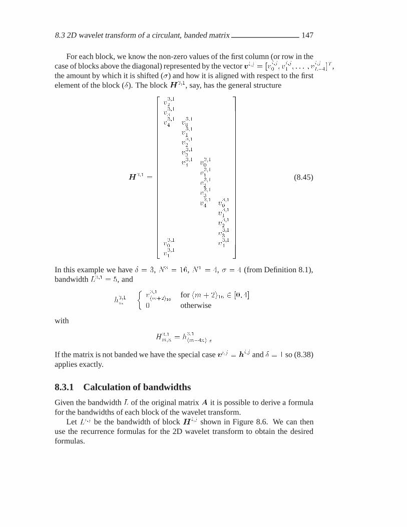
8.3 2D wavelet transform of a circulant, banded matrix 147
For each block, we know the non-zero values of the first column (or row in thecase of blocks above the diagonal) represented by the vector vi�j � vi�j� � vi�j� � � � � � vi�jL���
T ,the amount by which it is shifted (�) and how it is aligned with respect to the firstelement of the block (). The block H���, say, has the general structure
H��� �
������������������������������
v����
v����
v���� v����
v����
v����
v����
v���� v����
v����
v����
v����
v���� v����
v����
v����
v����
v���� v����
v����
������������������������������
(8.45)
In this example we have � �, N� � ��, N� � �, � � � (from Definition 8.1),bandwidth L��� � �, and
h���m �
�v���hm��i�� for hm� �i� � �� ��
� otherwise
with
H���m�n � h���hm��ni��
If the matrix is not banded we have the special case vi�j � hi�j and � � so (8.38)applies exactly.
8.3.1 Calculation of bandwidths
Given the bandwidth L of the original matrix A it is possible to derive a formulafor the bandwidths of each block of the wavelet transform.
Let Li�j be the bandwidth of block H i�j shown in Figure 8.6. We can thenuse the recurrence formulas for the 2D wavelet transform to obtain the desiredformulas.

148 2D Fast Wavelet Transform of a circulant matrix
Blocks on the diagonal
We start with the blocks on the diagonal given by equation (8.1) to (8.4) andconsider again only the cd block as the typical case. Let us recall (8.29):
hj���j��m � q�aahj�j�m �
D��Xp��
hqpaa h
j�jh�m�piNj
� qpaa hj�jh�m�piNj
i
for m � �� �� � � � � N j�� � �. Assume that hj�j is banded, i.e. zero outside aband of length Lj�j as shown in Figure 8.11. Then we can use the recurrenceformula to compute the bandwidth of hj���j��. Without loss of generality wemay assume that the nonzero part is wholly contained in the vector; i.e. there isno wrap-around.
Lj�j
hj�j m�
Figure 8.11: The band of hj�j has length Lj�j and starts at index m�.
Since hj�j is zero outside the interval starting at m� of length Lj�j , we seethat hj���j��m will be zero only if �m � p � m� � Lj�j or �m � p � m� for allp � ��D � ��. This leads immediately to the inequalities
�m� �D � �� � m�
�m� �D � �� � m� � Lj�j
or
m � m� � Lj�j �D � �
�or
m �m� �D � �
�
The length of this interval is then the bandwidth of hj���j��:
Lj���j�� �m� � Lj�j �D � �
�� m� �D � �
�
�Lj�j
��D � � (8.46)
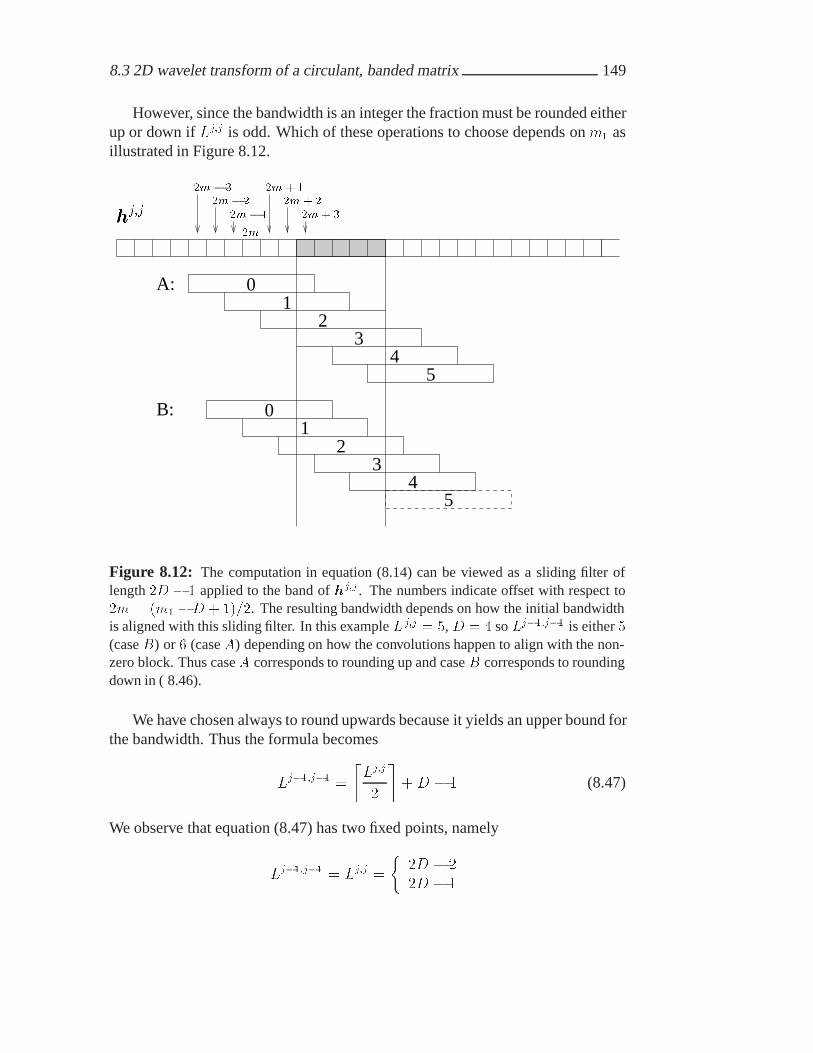
8.3 2D wavelet transform of a circulant, banded matrix 149
However, since the bandwidth is an integer the fraction must be rounded eitherup or down if Lj�j is odd. Which of these operations to choose depends on m� asillustrated in Figure 8.12.
0
4
12
3
0
5
12
34
5
�m
�m� �
�m� �
�m� �
�m� �
�m� �
�m� �
A:
B:
hj�j
Figure 8.12: The computation in equation (8.14) can be viewed as a sliding filter oflength �D � � applied to the band of hj�j . The numbers indicate offset with respect to�m � �m� �D � ���. The resulting bandwidth depends on how the initial bandwidthis aligned with this sliding filter. In this example L j�j � , D � � so Lj���j�� is either (case B) or � (case A) depending on how the convolutions happen to align with the non-zero block. Thus case A corresponds to rounding up and case B corresponds to roundingdown in ( 8.46).
We have chosen always to round upwards because it yields an upper bound forthe bandwidth. Thus the formula becomes
Lj���j�� ��Lj�j
�
��D � � (8.47)
We observe that equation (8.47) has two fixed points, namely
Lj���j�� � Lj�j �
��D � ��D � �

150 2D Fast Wavelet Transform of a circulant matrix
and it turns out that there is convergence to one of these values depending onwhether the initial Lj�j is smaller than �D � � or larger than �D � �. However,the important fact is that these fixed points are more related to the wavelet genusD than to the original bandwidth L.
Blocks below and above the diagonal
The bandwidths of the blocks below the diagonal are found from recurrence for-mulas of the form
hi�j��m �
D��Xl��
alhi�jhm��li
Ni
Again, we disregard wrapping and, proceeding as in the case of hj���j�� above,we find that hi�j��m is zero only if m � �l � m� � Li�j or m � �l � m� for alll � ��D � ��. This leads to the inequalities
m � m�
m� ��D � �� � m� � Li�j
Consequently, the interval length for which hi�j��m �� � is
Li�j�� � m� � Li�j � ��D � �� �m�
� Li�j � ��D � ��
Performing similar computations for blocks above the diagonal yields the re-sult
Li�j�� � Lj���i � Li�j � ��D � �� (8.48)
Since � is the ratio between N i and N j , equation (8.48) shows that the bandwidthgrows exponentially as the difference between i and j increases. Figures 8.13and 8.14 show examples of the bandwidths for different transform levels.

8.3 2D wavelet transform of a circulant, banded matrix 151
L � �
�
�
�
� �
� � �
�
�
�
�
� �
�
��
� �
�
�
�
�
�
�
��
�
��
� ��
� ��
Figure 8.13: The bandwidths for transform depths � � �� �� �� . The initial bandwidthis and D � �. These bandwidths are upper bounds since actual bandwidths may be oneless than the predicted values as can be seen in Figure 8.10.

152 2D Fast Wavelet Transform of a circulant matrix
� � ��
� �
�
�
�� �
�
�
�
�
�
��
��
�
��
��
� �� ��
� �� ��
Figure 8.14: The bandwidths for transform depth � � �.

8.4 Matrix-vector multiplication in a wavelet basis 153
8.4 Matrix-vector multiplication in a wavelet basis
We now turn to the problem of computing the matrix-vector product y � Hx
where x�y � RN and H is given as in (8.25). This system has the form shownin Figure 8.15.
H�� H�� H�� H��
H�� H�� H��
H�� H��
H��
H��
H��
H��
H��
H�� H��
H
x�
x�
x�
x�
x
�
y�
y�
y�
y�
y
Figure 8.15: The structure of y �Hx for � � .
154 2D Fast Wavelet Transform of a circulant matrix
The vector y may be computed block-wise as follows
yi ��X
j��
H i�jxj� i � �� �� � � � � � (8.49)
where � is the depth of the wavelet transform. The symbols xj , yi, and Hi�j
denote the different blocks of the x, y, and H as indicated in Figure 8.6. Thecomputation in (8.49) is thus broken down into the tasks of computing the prod-ucts which we will denote by
yi�j �H i�jxj� i� j � �� �� � � � � � � � (8.50)
In the following we distinguish between blocks on or below the diagonal (i � j)and blocks above the diagonal (i � j).
8.4.1 Blocks on or below the diagonal
Let vi�j , i � j, be the vector of length Li�j representing the nonzero part of thefirst column of H i�j , i.e.
hi�jm �
�vi�jhm� ��i
Nifor hm� � �iN i � �� Li�j � ��
� otherwise
and
H i�jm�n � hi�jhm��niNi
where m � �� �� � � � � N i, � � N i�N j , and is the offset relative to the upper leftelement (see (8.45)). From equation (8.50) we see that the typical element of yi�j
can be computed column wise as
yi�jm �N j��Xn��
H i�jm�nx
jn
�N j��Xn��
hi�jhm��niNixjn
�N j��Xn��
vi�jhm��n� ��iNixjn (8.51)
For each n this computation is only valid for those m � �� N i � �� wherevi�jhm��n� ��iNi
is defined, namely where
� � hm� �n� � �iN i � Li�j � � (8.52)

8.4 Matrix-vector multiplication in a wavelet basis 155
Let k and l be defined such that k � m � l whenever (8.52) is satisfied. Then wecan find k from the requirement
hk � �n� � �iN i � � k � h�n� � �iN i
and the last row as l � hk � Li�j � �iN i . Letting
yi�jk�l � yi�jk � yi�jk��� � � � � yi�jl �
then we can write the computation (8.51) compactly as
yi�jk�l � yi�jk�l � xjn vi�j��Li�j��� n � �� �� � � � � N j � � (8.53)
When k � l the band is wrapped and (8.53) must be modified accordingly.If the vector x is a wavelet spectrum then many of its elements are normally
close to zero as described in Chapter 4. Therefore we will design the algorithm todisregard computations involving elements in xj where��xjn�� � �
The algorithm is given below
Algorithm 8.2: yi�j Hi�jxj , i � j
For n � � to N j � �if jxjnj � � then
k � h�n� � �iN i
l � hk � Li�j � �iN i
if k � l thenyi�jk�l � yi�jk�l � xjnv
i�j
else (wrap)yi�j��l � yi�j��l � xjnv
i�jLi�j�l�L��
yi�jk�N i�� � yi�j
k�N i�� � xnvi�j��Li�j�l��
endend
end
8.4.2 Blocks above the diagonal
Let vi�j, i � j, be the vector of length Li�j representing the nonzero part of thefirst row of H i�j , i.e.
hi�jn �
�vi�jhn� ��iNj
for hn � � �iN j � �� Li�j � ��
� otherwise(8.54)

156 2D Fast Wavelet Transform of a circulant matrix
where
H i�jm�n � hi�jhn��miNj
(8.55)
with � � N j�N i. An example (shown for H���) is
������������
v�v� vvv�v� v�v v��� v�v�v�v�v�v� vvv�v� v�v v���
v�v�v�v� vvv�v� v�v v���
v�v�v�v� vvv�v� v�v v���v�v�v�v� vvv�v� v�v v���
v�v�v�v� vvv�v� v�v v���v��� v�v�v�v� vvv�v� v�v v�v� v�v v��� v�v�v�v� vv
������������
Here � � �� � �, N� � �, N� � ��, L��� � �� (padded with one zero). Thesuperscripts i� j has been dropped in this example.
In order to be able to disregard small elements in x as in the previous section,we would like to convert the row representation to a column oriented format. Asindicated in the example above, the block Hi�j can be characterized completelyby � column vectors each with length Li�j�� together with some book-keepinginformation. We will assume that Li�j is a multiple of �, possibly obtained throughpadding with zeros as suggested in the example above.
Now we choose these vectors from the columns
Li�j � � Li�j � � �� � � � � Li�j � � � � �
which are the � last columns where the top row is non-zero: the shaded area in theexample above. Let these column vectors be denoted Zi�j
��d for d � �� �� � � � � �� �.From (8.54) and (8.55) we get
Z i�jm�d � H i�j
m�Li�j� �d� hi�jhLi�j� �d��mi
Nj
� vi�jhLi�j� �d��m� ��iNj
� vi�jhLi�j��m�d��iNj
(8.56)
for m � �� �� � � � � Li�j�� � � and d � �� �� � � � � � � �. In the example above wehave
Z i�j��� �
"# �
v�v�
$A � Z i�j
��� �
"# v��
v v�
$A � Z i�j
��� �
"# v�
v�v�
$A � Z i�j
��� �
"# v�
v�v�
$A

8.4 Matrix-vector multiplication in a wavelet basis 157
Equation (8.50) can then be computed columnwise using Zi�j��d instead ofH i�j . The
typical element of yi�j is
yi�jm �
N j��Xn��
H i�jm�nx
jn
�N j��Xn��
Z i�js�dx
jn
Let k and l be defined such that k � m � l whenever � � s � Li�j�� � � andlet n be fixed. Our task is now to determine d, together with k and l, such thatZ i�js�d � H i�j
m�n. Therefore we put s � � and look for k, d such that
Z i�j��d � H i�j
k�n (8.57)
In other words: For n given, we want to know which vector to use and at whichrow it must be aligned.
Next we insert the definitions (8.55) and (8.56) in (8.57) and use (8.54) toobtain the equation
vi�jhLi�j�d��iNj� hi�jhn��ki
Nj� vi�jhn��k� ��i
Nj
which is fulfilled whenever
hLi�j � d � �iN j � hn � �k � � �iN j hLi�j � d� n� �k � iN j � �
Let L � Li�j � n� . Then we can write the requirement as
hL� d � �kiN j � � (8.58)
Since we need k in the interval �� N i � �� we rewrite (8.58) using Lemma B.2:
� � hL � d � �kiN j
� h�L� d � �k���iN j��
� hk � �L � d���iN i
from which we get
k � h�d � L���iN i
For this to be well-defined � must be a divisor in �d�L�, i.e. hd � Li� � � so wemust choose
d � hLi�

158 2D Fast Wavelet Transform of a circulant matrix
Expanding the expression for L we obtain the desired expressions
d � hLi�j � n� i� (8.59)
k � h�d� Li�j � n � ���iN i (8.60)
Finally, l is obtained as
l � hk � Li�j�� � �iN i (8.61)
Let Zi�js�d be defined by (8.56). Using (8.59), (8.60) and (8.61) we can formulate
the algorithm as
Algorithm 8.3: yi�j H i�jxj, i � j
For n � � to N j � �if jxnj � � then
d � hLi�j � n� i�k � h�d � Li�j � n� ���iN i
l � hk � Li�j�� � �iN i
if k � l thenyi�jk�l � yi�jk�l � xjnZ
i�j��d
else (wrap)yi�j��l � yi�j��l � xjnZ
i�jLi�j���l�Li�j�����d
yi�jk�N i�� � yi�jk�N i�� � xjnZi�j��Li�j���l���d
endend
end
8.4.3 Algorithm
The full algorithm for computing (8.49) is
Algorithm 8.4: Matrix-vector multiplication (CIRMUL)y � �For j � � to �
For i � � to �If i � j then
yi � yi � yi�j computed with Algorithm 8.2else
yi � yi � yi�j computed with Algorithm 8.3

8.4 Matrix-vector multiplication in a wavelet basis 159
8.4.4 Computational work
We are now ready to look at the computational work required for the matrix-vector multiplication y �Hx. We take (8.49) as the point of departure and startby considering the typical block
H i�jxj
The length of xj is N j so for blocks on and below the diagonal of H (i � j) inAlgorithm 8.2 there are Li�jN j multiplications and the same number of additions.Hence the work is
�Li�jN j
floating point operations. For blocks above the diagonal (j � i) in Algorithm 8.3there are N jLi�j�� � Li�jN i multiplications and additions, so the work here is
�Li�jN i
The total work can therefore be written as follows
�Xj��
�Lj�jN j ��Xi��
i��Xj��
�Li�jN j ��X
j��
j��Xi��
�Li�jN i
where the first sum corresponds to blocks on the diagonal, the second to blocksbelow the diagonal, and the third to blocks above the diagonal. Since Li�j � Lj�i
we can swap the indices of the last double sum to find the identity
�Xj��
j��Xi��
�Li�jN i ��Xi��
i��Xj��
�Li�jN j
Hence we may write the total work of the matrix-vector multiplication with thewavelet transform of a circulant matrix as
FCIRMUL � ��X
j��
Lj�jN j � ��Xi��
i��Xj��
Li�jN j (8.62)
We recall that
N j �
�N��� for j � �N����j�� for � � j � �

160 2D Fast Wavelet Transform of a circulant matrix
and that Li�j is given by the recurrence formulas
Lj���j�� � dLj�j��e �D � �
Li�j�� � Li�j � �i�j�D � ��
L������� � L (the bandwidth of the original matrix A)
Tables 8.2, 8.3, and 8.4 show FCIRMUL evaluated for various values of L, D, �, andN .
� � �� L � �N D � � D � � D � � D � ��� ��� ���� ���� ������ ���� ���� ���� ������� ���� ���� ���� �������� ���� ����� ����� �������� ����� ����� ����� ��������� ����� ����� ����� ��������� ����� ����� ������ ������
Table 8.2: The number of floating point operations FCIRMUL as a function of N fordifferent values of D.
N � ����D � �� L � � L � � L � � L � �� ���� ���� ���� ����� ���� ���� ���� ����� ���� ���� ���� ����� ����� ����� ����� ������ ����� ����� ����� ������ ����� ����� ����� �����
Table 8.3: The number of floating point operations FCIRMUL shown for different valuesof � and L. Note that L � �k and L � �k � � (k � N) yield the same values for � �.This is a direct consequence of the rounding done in (8.62).

8.5 Summary 161
N � ���� L � �� D � � D � � D � � D � �� ���� ���� ���� ����� ���� ���� ���� ������ ���� ���� ����� ������ ���� ����� ����� ������ ���� ����� ����� ������ ���� ����� ����� �����
Table 8.4: The number of floating point operations FCIRMUL shown for different valuesof � and D.
Table 8.2 shows that FCIRMUL depends linearly on N . Moreover, Tables 8.3and 8.4 show that the computational work grows with the bandwidthL, the waveletgenus D, and the transform depth �. Suppose that L is given. Then we see thatthe matrix-vector multiplication is most efficient if we take no steps of the wavelettransform (� � �). Consequently, any work reduction must be sought in trunca-tion of the vector x. This can be justified because x will often be a 1D wavelettransform of the same depth (�) as the matrix H . Therefore, depending on � andthe underlying application, we expect many elements in x to be close to zero sowe may be able to discard them in order to reduce the computational work. Con-sider Table 8.3. If we take N � ���, L � �, � � � as an example, the questionboils down to whether such a truncation of x can reduce 14592 operations to lessthan the 1536 operations required for � � � (no transform). Assuming that thework depends linearly on the number of non-zero elements in x, this means that xmust be reduced by a factor of �� (at least) before any work reduction is obtained.
8.5 Summary
We have derived an algorithm for computing the 2D wavelet transform of a circu-lant N �N matrixA in O�N� steps. More specifically we derived the bound
FCIRFWT�N� � �DN�� � ��
The algorithm works with a data structure that requires no more than ��N ele-ments instead of N�. If A is also banded the storage requirements are reducedfurther. Then we have shown how a banded matrix-vector multiplication usingthe proposed storage scheme can be implemented and the complexity of this al-

162 2D Fast Wavelet Transform of a circulant matrix
gorithm was analyzed. It was found that the work needed to compute the matrix-vector multiplication is linear in N and grows with the bandwidth (L), the waveletgenus (D), and the depth of the wavelet transform �. On the other hand, the workis reduced when small elements in x are discarded.
Chapter 9
Examples of wavelet-based PDEsolvers
We consider here the task of solving partial differential equations in one spacedimension using wavelets. We assume that the boundary conditions are periodicand make use of the periodized wavelets described in Section 2.3 and the materialdeveloped in Chapters 7 and 8. Sections 9.1 and 9.2 treat linear problems andserve to set the stage for Sections 9.3 and 9.4 which deal with nonlinear problems.
We begin by considering a periodic boundary value problem because it is asimple and illustrative example.
9.1 A periodic boundary value problem
Consider the 1D Helmholtz equation
�u�� � �u � f�x�u�x� � u�x� ��
�x � R (9.1)
where � � R and f�x� � f�x� ��.We look for �-periodic solutions, so it suffices to consider u�x� on the interval
� � x � �.
9.1.1 Representation with respect to scaling functions
We begin the discretization of (9.1) by replacing u�x� with the approximation
uJ�x� ��J��Xk��
�cu�J�k ��J�k�x�� J � N� (9.2)

164 Examples of wavelet-based PDE solvers
Following the approach that lead to (7.9) we find that
u��J�x� ��J��Xk��
�c���u �J�k ��J�k�x� (9.3)
where �c���u �J�k is given as in (7.12), i.e.
�c���u �J�k � D���cu�k �D��X
n���D�cu�J�hn�ki�J �
Jd dn� k � �� �� � � � � �J � �
with dn defined in (7.1).We can use the Galerkin method to determine the coefficients �cu�J�k. Multi-
plying (9.1) by ��J�l�x� and integrating over the unit interval yields the relation
�Z �
�
u��J�x���J�l�x� dx� �
Z �
�
uJ�x���J�l�x� dx �
Z �
�
f�x���J�l�x� dx
Using (9.2), (9.3), and the orthonormality of the periodized scaling functions(2.48) we get
��c���u �J�l � ��cu�J�l � �cf �J�l� l � �� �� � � � � �J � �
where
�cf �J�l �
Z �
�
f�x���J�l�x� dx (9.4)
In vector notation this becomes
�c���u � �cu � cf (9.5)
and using (7.13) we arrive at the linear system of equations
Acu � cf (9.6)
where
A � �D��� � �I (9.7)
Alternatively, we can replace D��� by D�, where D is given in (7.14), and obtain
Acu � cf (9.8)
where
A � �D� � �I (9.9)
Equations (9.6) and (9.8) represent the scaling function discretizations of (9.1).Hence this method belongs to Class � described in Section 7.1. We observe that(9.6) has a unique solution if � does not belong to the set of eigenvalues of D���.Similarly (9.8) has a unique solution if � does not belong to the set of eigenvaluesof D�.

9.1 A periodic boundary value problem 165
� log��ku� uJkJ���
A � �D��� � �I A � �D� � �IJ D � � D � � D � � D � � D � �� ���� ���� ���� ���� ����� ���� ���� ���� ���� ������ ���� ����� ���� ����� ������ ����� ����� ����� ����� ������ ����� ����� ����� ����� ������ ����� ����� ����� ����� ������ ����� ����� ����� ����� ������ ����� ����� ����� ����� �����
Table 9.1: The error � log��ku� uJkJ�� shown for different values of J , D and thechoice of differentiation matrix. Convergence rates are seen from the differences betweensuccessive measurements. The value D � � is omitted in the case of (9.7) because thecombinationD � �� d � � is invalid as described in Remark 7.1.
Accuracy
Let f�x� � ���� � �� sin���x�. The solution of (9.1) is then
u�x� � sin���x�
Define
kuk� � max��x��
ju�x�j (9.10)
kukJ�� � maxk����� ��J��
��u�k��J ��� (9.11)
Table 9.1 shows how the error ku� uJkJ�� depends on J , D, and the choice
of D��� or D�. Until the onset of rounding errors, the convergence rates obtainedin Chapter 7 are recovered. More precisely,
ku� uJkJ�� � O ���J�D���
�in the case of (9.7)
ku� uJkJ�� � O ���JD
�in the case of (9.9)
Table 9.2 shows how the error ku� uJk� depends on J , D, and the choice ofD��� or D�. In this case, we find
ku� uJk� � O ���JD��
�in the case of (9.7)
ku� uJk� � O ���JD��
�in the case of (9.9)

166 Examples of wavelet-based PDE solvers
� log��ku� uJk��
A � �D��� � �I A � �D� � �IJ D � � D � � D � � D � � D � �� ���� ���� ���� ���� ����� ���� ���� ���� ���� ����� ���� ���� ���� ���� ����� ���� ����� ���� ���� ������ ����� ����� ���� ����� ������ ����� ����� ����� ����� ������ ����� ����� ����� ����� ������ ����� ����� ����� ����� �����
Table 9.2: The error � log��ku� uJk� shown for different values of J , D and thedifferentiation matrix. Convergence rates are seen from the differences between succes-sive measurements. The value D � � is omitted in case of (9.7) because the combinationD � �� d � � is invalid as described in Remark 7.1.
which agrees with the approximation properties described in (4.5).The high convergence observed in Table 9.1 means that the solution u�x� is
approximated to Dth order in the norm k�kJ�� even though the the subspace �VJcan only represent exactly polynomials up to degree D�� � �, as explained inSection 4.1. This phenomenon, known as super convergence, is also encounteredin the finite element method, [WM85, p. 106], [AB84, p. 231].
9.1.2 Representation with respect to wavelets
Taking (9.6) as point of departure and using the relations
du � Wcu
df � Wcf
yields
AW Tdu �W Tdf
Let
�A �WAW T �W��D��� � �I
�W T � � �D
���� �I

9.1 A periodic boundary value problem 167
where �D���
is defined according to (7.22). Then
�Adu � df (9.12)
which is the wavelet discretization of (9.1). This method belongs to Class � de-scribed in Section 7.1. Hence, there is a potential for using wavelet compressionto reduce the computational complexity of solving (9.12).
9.1.3 Representation with respect to physical space
Multiplying (9.5) by T and using (3.17) yields
�u��� � �u � f
where
f � Tcf �%�PVJ
f��xl�
&�J��l��
(9.13)
From the relation u��� �D���u (7.15) we obtain the equation
Au � f (9.14)
where A is given by (9.7).An important variant of (9.14) is obtained by redefining f as the vector
f � ff�xl�g�J��l��
This produces a collocation scheme for the solution of (9.1).Because this method is essentially based on scaling functions and does not use
wavelet compression it belongs to Class � described in Section 7.1.
9.1.4 Hybrid representation
We mention a second possibility for discretizing (9.1) using wavelets. It is simpleand several authors follow this approach, e.g. [EOZ94, CP96, PW96]. This isessentially a combination of the approaches that lead to (9.14) and (9.12), and weproceed as follows: Multiplying (9.14) from the left by W and using the identityW TW � I one obtains
WAW TWu �Wf

168 Examples of wavelet-based PDE solvers
Defining the wavelet transformed vectors as
�f � Wf and
�u � Wu
then yields
�A�u � �f (9.15)
where �A is the same as in (9.12).This approach bypasses the scaling coefficient representation and relies on the
fact that the FWT can be applied directly to function values of f . Indeed, usingthis approach, the differentiation matrix A might as well be derived from finitedifferences, finite elements or spectral methods.
From Section 4.3 we know that the elements in �u will behave similarly as thetrue wavelet coefficients du. Therefore, wavelet compression is as likely in thiscase as with the pure wavelet representation (9.12). Hence this method belongs toClass � described in Section 7.1.
9.2 The heat equation
We consider now the periodic initial-value problem for the heat equation
ut � �uxx � f�x�� t � �u�x� �� � h�x�u�x� t� � u�x� �� t�� t � �
./0 x � R (9.16)
where � is a positive constant, f�x� � f�x � �� and h�x� � h�x � ��. Thediscretization strategies are time-dependent analogues of those in Section 9.1.
9.2.1 Representation with respect to scaling functions
We consider first the Galerkin method for (9.16) and proceed as in Section 9.1.1.The time-dependent version of (9.2) is
uJ �x� t� �
�J��Xk��
�cu�J�k�t���J�k�x� (9.17)
After an analysis similar to that which lead to (9.5), we arrive at the Galerkindiscretization of (9.16):
d
dtcu�t� � �D���cu�t� � cf � t � �
cu��� � ch
(9.18)

9.2 The heat equation 169
where cf is given by (9.4) and
�ch�J�k �
Z �
�
h�x���J�k�x� dx� k � �� �� � � � � �J � � (9.19)
9.2.2 Representation with respect to wavelets
Multiplying (9.18) from the left by W and inserting the identity W TW � I
yields
d
dtWcu�t� � �WD���W TWcu�t� �Wcf � t � �
From the identities
du�t� � Wcu�t�
df�t� � Wcf �t�
�D���
� WD���W T
we then obtain
d
dtdu�t� � � �D
���du�t� � df � t � � (9.20)
with the initial condition
du��� �Wch
9.2.3 Representation with respect to physical space
Proceeding as above but this time multiplying (9.18) from the left by T yields
d
dtTcu�t� � �TD���T��Tcu�t� � Tcf � t � �
Using the relations
u�t� � Tcu�t�
f � Tcf �%�PVJ
f��xl�
&�J��l��
D��� � TD���T��
we find
d
dtu�t� � �D���u�t� � f � t � � (9.21)

170 Examples of wavelet-based PDE solvers
with the initial condition
u��� � h �%�PVJ
h��xl�
&�J��l��
(9.22)
Also in this case we can produce a collocation scheme by redefining
f � ff�xl�g�J��l��
h � fh�xl�g�J��l��
9.2.4 Hybrid representation
Multiplying (9.21) from the left withW and proceeding as in Section 9.1.4 yields
d
dt�u�t� � � �D
����u�t� � �f � t � � (9.23)
with the initial condition
�u��� �Wh
9.2.5 Time stepping in the wavelet domain
A number of time-stepping schemes are available for the system (9.20). We con-sider here the backward Euler method defined by
�du�n�� � �du�n�t
� � �D����du�n�� � df (9.24)
where �du�n � du�n�t�. This leads to the recursion
�du�n�� � �A��
��du�n ��tdf � � n � �� �� � � � � n� � �
�du�� � du���(9.25)
where n� � N and
�A � I � ��t �D���
The backward Euler time-stepping schemes for (9.18), (9.21), and (9.23) are com-pletely analogous.
The matrix �A has the characteristic “finger-band” pattern shown in Figure 7.1,
and it turns out that so does �A��
for small �t when small entries are removed[CP96]. Figure 9.1 shows an example of �A
��where elements smaller than �����
have been removed.

9.2 The heat equation 171
0 512 1024
0
512
1024
nz = 125056
Figure 9.1: �A��
where elements smaller than ����� have been removed. D � �, � � ,J � ��, �t � ����, and � � ��� �.
Moreover, we can expect many elements in du and df to be small by virtueof Theorem 2.5. Consequently, there is a potential for compression of both thecoefficient matrix as well as the solution vector. This is true for both (9.20) and(9.23) but we give the algorithm for (9.20) only since the case (9.23) is completelyanalogous.
Let trunc�d� �� be a function that returns only the significant elements in agiven vector d, i.e. let
trunc�d� �� � fdj�k� jdj�kj � �gSimilarly, let
trunc�A� �� � fA�m�n� jA�m�nj � �gLet �V be the compression threshold for the vector and �M be the compressionthreshold for the matrix and define d�V � trunc�d� �V � and �A
�M� trunc� �A� �M�.
Following ideas given in [CP96] we can now give a computational procedurefor computing (9.25) using wavelet compression.
Algorithm 9.1
� � � �A����M � trunc �WA��W T � �M �
� � d�Vf � trunc �Wcf � �V �
� � �du��V� � trunc �Wch� �V �

172 Examples of wavelet-based PDE solvers
for n � �� �� � � � � n� � �
� � �du�n�� � � �A����M
��du��Vn ��td�Vf
�� � �du�
�Vn�� � trunc ��du�n��� �V �
end
� � �cu�n� � W T �du��Vn�� � �u��M ��V
n�� T �cu�n�
A few comments are appropriate:
� Step : We have
�A��
��WAW T
�����W T
���A��W �� �WA��W T
Hence, step � can be done using the 2D FWT (3.38). However, since A iscirculant thenA�� is also circulant by Theorem C.6 and it can be computed
efficiently using the FFT as explained in Appendix C. Consequently, �A��
can be computed and stored efficiently using Algorithm 8.1.
� Steps � �: ch, cf are both computed according to (3.17), i.e. by the quadra-ture formulas
cf � T��f
cu � T��h
where
f � ff�xk�g�J��k��
h � fh�xk�g�J��k��
� Step : It is essential for the success of this algorithm that the computationof the matrix-vector product fully exploits the compressed form of bothmatrix and vectors. This can be done, for example, using Algorithm 8.4.In [CP96, p. 7] fast multiplication is based on a general sparse format forboth matrix and vector.
� Steps �� �: Finally, the computed vector of wavelet coefficients is trans-formed back into the physical domain. We denote the computed solutionu�M ��Vn�
, because it depends on both thresholds.

9.2 The heat equation 173
To test Algorithm 9.1 we have applied it to the problem
ut � �uxx � sin���x�� t � �u�x� �� � �
�x � R (9.26)
The numerical parameters are J � ��, �t � �����, n� � ��� (making � � t � �),� � ������, � � �, and D � �. The vector u�M ��V
n�is the result of Algorithm 9.1
given the thresholds �M and �V . Hence, we define the relative compression erroras
E�M ��V �
''u�M ��Vn�
�u���n�
''�''u���
n�
''�
where
kuk� � maxk����� ��J��
julj
Table 9.3 shows the percentage of significant elements in ��A����M and �du��Vn�
for various values of �V and �M . Moreover, the relative error introduced by com-pression E�M ��V is given for each case. It is seen that significant compression canbe achieved in both the matrix and the solution vector.
�V � � % elem �M � � % elem
�M � �A����M E�M ��V �V �du��Vn� E�M ��V
����� ����� ����� ����� ����� �����
����� ����� ����� ����� ����� �����
���� ����� ������ ���� ����� ����
���� ����� ���� ���� ����� ����
���� ���� ����� ���� ����� ����
��� ���� ��� ��� ���� ���
���� ���� ����� ���� ���� ����
Table 9.3: Percentage of elements retained in � �A��
�M and �du�Vn� together with theresulting compression error.

174 Examples of wavelet-based PDE solvers
9.3 The nonlinear Schrodinger equation
We consider now the periodic initial-value problem for the nonlinear Schrodingerequation:
ut � Lu� i juj� u� t � �u�x� �� � h�x�u�x� t� � u�x� L� t�� t � �
./0 x � R (9.27)
where h�x� � h�x� L� and
L � � i
���
��
�x�� �
�
This equation describes the propagation of a pulse envelope in an optical fiber. ��is a dispersion parameter, � is a measure of intensity loss, and is the magnitudeof the nonlinear term which counteracts dispersion for certain waveforms [Agr89,FJAF78, LBA81, PAP86]. Sometimes the term �
��
��
�x�, which represents third
order dispersion, is added to L.Because of periodicity we can restrict the spatial domain of (9.27) to the inter-
val �L��� L��. Let N � �J and define a grid consisting of the points
xl �
l
N� �
�
L� l � �� �� � � � � N � �
Define the vector u�t� such that
ul�t� � uJ�xl� t�� l � �� �� � � � � N � �
where uJ�x� t� is an approximate solution of (9.27) of the form (9.17). Definesimilarly the vectors u����t� and f �t� as
u���l �t� � u��J�xl� t�� l � �� �� � � � � N � �
fl�t� � f�xl� t�� l � �� �� � � � � N � �
Hence the elements inu approximate function values of u in the interval �L��� L��.With regard to our using the interval L��� L�� instead of �� � we mention thatthe mappings Tc and Wc are unchanged as described in Section 3.2.4 but thedifferentiation matrix must be scaled according to (7.18). Hence, we arrive at thefollowing initial problem for u formulated with respect to physical space:
d
dtu�t� � Lu�t� �N �u�t�� u�t�� t � �
u��� � h h�x��� h�x��� � � � � h�xN����T(9.28)
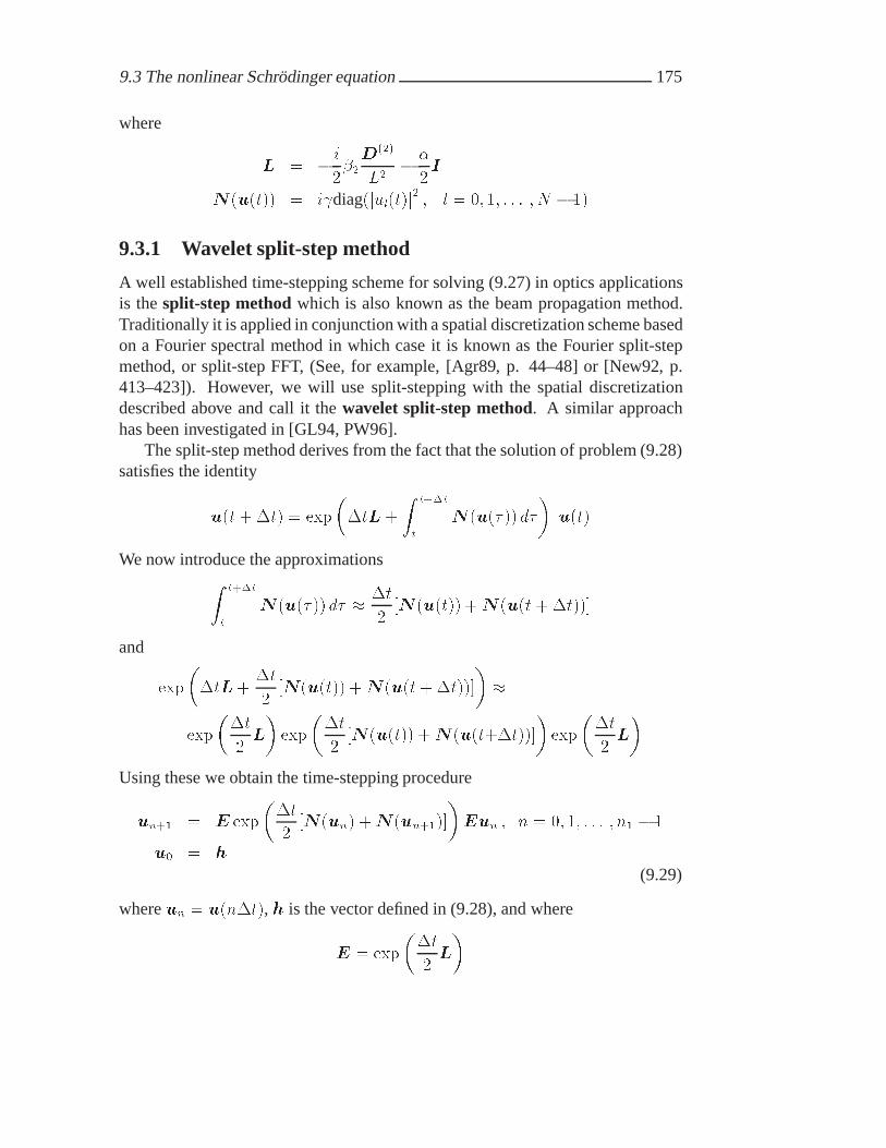
9.3 The nonlinear Schrodinger equation 175
where
L � � i
���D���
L�� �
�I
N �u�t�� � idiag�jul�t�j� � l � �� �� � � � � N � ��
9.3.1 Wavelet split-step method
A well established time-stepping scheme for solving (9.27) in optics applicationsis the split-step method which is also known as the beam propagation method.Traditionally it is applied in conjunction with a spatial discretization scheme basedon a Fourier spectral method in which case it is known as the Fourier split-stepmethod, or split-step FFT, (See, for example, [Agr89, p. 44–48] or [New92, p.413–423]). However, we will use split-stepping with the spatial discretizationdescribed above and call it the wavelet split-step method. A similar approachhas been investigated in [GL94, PW96].
The split-step method derives from the fact that the solution of problem (9.28)satisfies the identity
u�t��t� � exp
�tL�
Z t�t
t
N �u�� �� d�
u�t�
We now introduce the approximationsZ t�t
t
N �u�� �� d� � �t
�N �u�t�� �N �u�t��t���
and
exp
�tL�
�t
�N�u�t�� �N �u�t��t���
�
exp
�t
�L
exp
�t
�N�u�t�� �N �u�t��t���
exp
�t
�L
Using these we obtain the time-stepping procedure
un�� � E exp
�t
�N�un� �N �un����
Eun � n � �� �� � � � � n� � �
u� � h
(9.29)
where un � u�n�t�, h is the vector defined in (9.28), and where
E � exp
�t
�L

176 Examples of wavelet-based PDE solvers
The vector un�� appears also on the right-hand side of (9.29) so each time steprequires an iterative procedure. Ours is the following: For each n let
u���n�� � un
and iterate until convergence,
u�q���n�� � E exp
�t
�N �un� �N �u
�q�n����
Eun� q � �� �� � � �
Defining the function
linstep�v� � Ev
we have the following algorithm for (9.29):
Algorithm 9.2: Split-step method
�: u� � h � fh�xk�g�J��k��
�: E � exp�t� L
��: N � �N �u��
for n � �� �� � � � � n� � �
�: vn � linstep�un�
�: N � �N �
Iterate until convergence�: un�� � linstep
�exp
�t� N� �N ��
�vn�
�: N � �N �un���
9.3.2 Matrix exponential of a circulant matrix
N �un� is a diagonal matrix for every value of n, so the exponentiation required instep � of Algorithm 9.2 can be done cheaply. The matrix L, on the other hand, isnot diagonal but it is circulant. Hence, with regard to step �, we need a procedurefor computing the matrix exponential
E � eA (9.30)
where A is the circulant matrix
A ��t
�L

9.3 The nonlinear Schrodinger equation 177
Standard methods for computing (9.30) are mostly based on matrix multiplica-tions [GL89] which have complexity O �N��. Hence the computation of (9.30)can be very expensive.
However, by using the fact that A is circulant one can compute (9.30) inO�N log�N� floating point operations. From Theorem C.4 we have the factor-ization
A � F��N �aFN
where F N is the Fourier matrix defined in (C.3), �a � diag�a�, a � FNa, anda is the first column in A. By a standard matrix identity
E � exp�A� � F��N exp�FNAF
��N �FN � F��
N exp��a�F N
The matrix exp��a� is diagonal so we know from Theorem C.4 thatE is circulant.Hence we can write
E � F��N �eFN
where �e � diag�e�, e � F Ne, and e is the first column in E. Equating �e andexp��a� yields
e � e�a�� e�a�� � � � � e�aN���T
Hence we have the following fast algorithm for computing (9.30):
Algorithm 9.3: Exponential of circulant matrixA
a � A���� ! Extract first column of Aa � FNa ! FFTe � fexp�ak�gN��k�� ! Pointwise exponentiatione � F��
N e ! IFFTE�m�n � ehm�niN � m� n � �� �� � � � � N � � ! Assemble E
The matrices A and E need not be stored explicitly. Hence the first and thelast steps here can be omitted in practice. In step � of Algorithm 9.2, where weuse Algorithm 9.3, only e is computed. The computational complexity followsfrom that of the FFT and its inverse.
In the problem at hand A � t� L, where L is circulant and banded. It follows
from the definition of the matrix exponential
E � exp�A� ��Xk��
Ak�k� (9.31)

178 Examples of wavelet-based PDE solvers
that E is dense. However, it turns out that many entries in E are very small andthatE assumes circulant band form if truncated with a small threshold. In [GL94,PW96] E is approximated by truncating the series (9.31) to a few terms. Thisalso yields a circulant band form, but the process is less exact and not significantlyfaster than the one presented here.
9.3.3 Compression
We can exploit the compression potential of wavelets by an appropriate imple-mentation of linstep. Let
�E �WEW T (9.32)
and
� �E��M � trunc� �E� �M�
Then the product Ev that is computed by linstep can be formulated as
Ev �W T �EWv �W T �E�v �W T � �E��M �v�V
where �v�V � trunc��v� �V �. Hence we obtain the following version of linstepwhich can be used in step � and � of Algorithm 9.2.
Algorithm 9.4: u� linstep�v�
�v � Wv
��v��V � trunc��v� �V �
�u � � �E��M ��v��V
u � W T �u
Since E is circulant, �E can be computed efficiently using Algorithm 8.1.Since E is dense �E is dense too, but under truncation, even with very smallthresholds, it assumes the finger-band pattern associated with differential oper-ators in wavelet bases. Figure 9.2 shows �E truncated to machine precision for� � �� �� �� �� �� �, the case � � � corresponding to E .

9.3 The nonlinear Schrodinger equation 179
0 256
0
256
nz = 5888
λ=0
0 128 256
0
128
256
nz = 9728
λ=1
0 64 128 256
0
64
128
256
nz = 12928
λ=2
0 32 64 128 256
0
32
64
128
256
nz = 16320
λ=3
0 16 32 64 128 256
01632
64
128
256
nz = 19648
λ=4
0 16 32 64 128 256
01632
64
128
256
nz = 22800
λ=5
Figure 9.2: �E�M for � � �� �� �� � �� truncated to the precision �M � ����������� .
The remaining parameters are D � �, J � �, �t � �����, L � ��, � � ��, and � � �.

180 Examples of wavelet-based PDE solvers
% elem. retained
� �E�M
��E���M
� ���� ������ ����� ������ ����� ������ ����� ������ ����� ������ ����� �����
Table 9.4: The percentage of elements retained in �E�M and � �E
��M for �M � �������
���� , D � �, J � �, �t � �����, L � ��, � � ��, � � �. It is seen that thecompression potential of �E
�is slightly lower than that of �E.
Recall from Chapter 7 that the differentiation process has higher convergenceif D��� is replaced by D�, but that this comes at the cost of a larger bandwidth.We want to compare these two choices with respect to compression potential. Let
L� � � i
���D�
L�� �
�I
E� � exp
�t
�L�
�E�
� WE�W T
The percentages of elements retained in �E and �E�
with truncation to machineprecision are shown in Table 9.4 for � � �� �� �� �� �� �.
Figure 9.3 shows �E�M
for different choices of �M and Table 9.5 shows thecorresponding percentages of elements retained in �E and �E
�. It is observed that
the compression potential of E� is slightly lower than that of E, so we will useonly E in the following.

9.3 The nonlinear Schrodinger equation 181
0 32 64 128 256
0
32
64
128
256
nz = 4992
εM
=0.0001
0 32 64 128 256
0
32
64
128
256
nz = 11008
εM
=1e−07
0 32 64 128 256
0
32
64
128
256
nz = 13504
εM
=1e−10
0 32 64 128 256
0
32
64
128
256
nz = 14976
εM
=1e−13
Figure 9.3: �E�M for �M � ����� ����� ������ �����. The remaining parameters are
D � �, J � �, � � , �t � �����, L � ��, � � ��, and � � �.
% elem. retained
�M �E�M
��E���M
���� ���� �������� ����� ���������� ����� ���������� ����� �����
Table 9.5: The percentage of elements retained in �E�M and � �E
��M for �M �
����� ����� ������ �����. The remaining parameters are D � �, J � �, � � ,�t � �����, L � ��, � � ��, and � � �. Hence, the first column corresponds tothe matrices shown in Figure 9.3.

182 Examples of wavelet-based PDE solvers
Thresholds % elem. retained�M �V E�M ��V �E
�M�u�Vn� CPU time (s)
� � ���� � ��� ��� ��� �������� � ���� � ��� �� ��� �������� ����� ���� � ��� � ��� �������� ����� ���� � ��� � �� �������� ���� ���� � ��� � �� �������� ���� ���� � ��� � �� �������� ��� ���� � ���� � �� ���
Table 9.6: Error, compression and execution time data for a problem with known solu-tion (compression of �un� is given for n� � ����).
The wavelet split-step method as defined by Algorithm 9.2 and the implemen-tation of linstep given in Algorithm 9.4 has been implemented in Fortran 90 ona CRAY C92A. Algorithm 9.3 was used for computing the matrix exponentialE � exp
�t� L
�, Algorithm 8.1 was used for (9.32) using the data structure de-
scribed in Section 8.2.5, and Algorithm 8.4 was used for computing the product
� �E��M ��v��V
Finally, the transformsWv and W T �v were implemented using the FWT and theIFWT defined in Section 3.3. Hence, the algorithm has the complexity O�N�regarding both storage and floating point operations.
To test the performance of this algorithm, we have applied it to a case ofproblem (9.27) with a known solution. The data are �� � ��, � � �, � �and h�x� � eixsech�x�, which yield the solution u�x� t� � eixsech�x � �t�. Thenumerical data are L � ��, J � �� (making N � ����), � � �, n� � ����, and�t � �����. The wavelets used were those of genus D � �. Table 9.6 shows therelative error, percentage of compression achieved in �E and �un� , and measuredCPU time of n� time steps as functions of the threshold parameters �M and �V .The relative error is defined here as
E�M ��V �maxk����� ��J�� jun� �k � u�xk� ��j
maxk����� ��J�� jun� �kj
It is seen that wavelet compression in this case can yield a speedup of about sevenwith a relative error of about �� ����.

9.3 The nonlinear Schrodinger equation 183
% elem. retained� �E
�M�u�Vn� CPU time (s)
� ���� ����� ��� ���� ����� ��� ���� ����� ���� ���� ����� ���� ���� ����� ���� ���� ����� ���� ���� ����� ���� ���� ����� ���
Table 9.7: Compression ratios of �E and �un� (n� � ����) and execution time in (CPUseconds) of the wavelet split-step algorithm for different values of �. Here �M � �����
and �V � ����.
Table 9.7 shows how performance depends on the transform depth �. It isseen that even though the compression potential of �un� increases with �, it isnot enough to balance the increased work inherent in the matrix vector multi-plications. This should be compared to Table 8.3 which indicates that the workgrows with � unless �un� is compressed excessively. The gain from compressionis outweighed by the cost of the wavelet transform in Algorithm 9.4. and that ofcomputing Algorithm 8.4.
To illustrate a realistic application, we show in Figure 9.4 a computed “breathersolution” obtained from the data �� � ��, � � �, � �, h�x� � �sech�x�,L � ��, N � ����, � � �, �t � ����� and D � �. The figure gives only themiddle third of the x-interval.

184 Examples of wavelet-based PDE solvers
0
1
2
−100
10
0
5
10
15
x
t
|u|2
Figure 9.4: A “breather solution” of problem (9.27).

9.4 Burgers’ equation 185
9.3.4 FFT split-step method
To assess the performance of the wavelet split-step method we compare it to animplementation of the FFT split-step method which is the de facto standard forsolving the nonlinear Schrodinger equation [New92].
The FFT split-step method exploits the fact that the Fourier differentiationmatrixD�d�
F , given in Appendix D, is diagonal. Hence,
LF � � i
���D
���F
L�� �
�I
is diagonal and
E � exp��t
�LF � (9.33)
is also diagonal. The FFT split-step algorithm is therefore given by Algorithm 9.2but with step � replaced by (9.33) and linstep�v� (used in steps � and �) redefinedas
Algorithm 9.5: u� linstep�v�
v � FNv
u � Ev
u � F��N u
The product Ev is computed in N operations so the complexity for large Nis dominated by that of the FFT and hence is O�N log�N�. This should be com-pared to the wavelet split-step method where the FWT as well as the matrix-vectorproduct has linear complexity, the latter, however, involving a large constant.
Replacing Algorithm 9.4 by Algorithm 9.5 renders Algorithm 9.2 the FFTsplit-step method. The performance of the FFT split-step method with the sameparameters as in Table 9.6 yields an execution time of ��s with a relative errorof ���� � ��� . The FFT routine used for this purpose was a library routineoptimized for vectorization on the CRAY C92A. In contrast, the implementationof Algorithm 8.4 did not vectorize well due to short vector lengths and inefficientmemory access. Table 9.8 shows how the execution time grows with N for theFFT split-step method and the wavelet split-step method. In the wavelet case theparameters are D � �, � � �, �M � �����, and �V as given in the table.
9.4 Burgers’ equation
We consider now Burgers’ equation which is frequently used to study adaptivemethods because it models formation of shocks. The periodic initial-value prob-

186 Examples of wavelet-based PDE solvers
CPU time (s)N FFT �V � ���� �V � ����
��� � �� ����� � �� ����� � �� ������ � ��� ������ �� ��� ������� �� ��� ������� �� ��� �������� �� ���� ���
Table 9.8: Execution time (CPU seconds) for the FFT split-step method and the waveletsplit-step method both applied to (9.27). The latter method is shown for two differentcompression thresholds.
lem for a particular form of Burgers’ equation is
ut � �uxx � �u� �ux� t � �u�x� �� � h�x�u�x� t� � u�x� �� t�� t � �
./0 x � R (9.34)
where � is a positive constant, � R and h�x� � h�x � ��. Burgers’ equationwith � � describes the evolution of u under nonlinear advection and lineardissipation. A nonzero value of adds linear advection to the system.
This problem is discretized in the same manner as (9.42), and we obtain thesystem
d
dtu�t� � Lu�t� �N �u�t�� u�t�� t � �
u��� � h h�x��� h�x��� � � � � h�xN����T
where
L � �D��� � I
N �u�t�� � �diag�Du�t��
withD �D���. This has the same form as (9.28) and an appropriate modificationof Algorithm 9.2 can be used to solve it.
The matrix-vector product u��� � Du can be computed analogously to thecomputation of the matrix-vector multiplications in Algorithm 9.4. Hence wehave

9.4 Burgers’ equation 187
Algorithm 9.6: u��� �Du
�u � Wu
��u��V � trunc��u� �V �
�u��� � � �D��D ��u��V
u��� � W T �u���
where �D �WDW T and
� �D��D � trunc� �D� �D�
UnlikeE, which is dense, the matrixD is a banded matrix (see Section 7.3) so �Dwill have the “finger band” structure without applying any compression. However,the wavelet transform introduces rounding errors which we remove by choosing�D to be a fixed small precision, namely �D � �����, as this is sufficient to retainthe sparsity of �D. Hence we use Algorithms 8.1 and 8.4 for computing �D and theproduct � �D��D ��u��V , respectively.
To test this procedure on (9.34) we have chosen the values � � �����, � �,and h�x� � sin���x�. The numerical data are J � ��, � � �, �M � �����,�V � �����, �t � �����, n� � ���, and D � �. The implementation was donein Fortran 90 on a 200 MHz PC using the Linux operating system.
Figure 9.5 shows the evolution of u�x� t� for � � t � ���. It is seen that alarge gradient forms at x � ��� whereas u is very smooth elsewhere. Hence weexpect a large wavelet compression potential.
Table 9.9 shows the influence on performance of the parameter �V with �M(and �D) fixed. It is seen that the execution time drops as fewer elements are re-tained in �un� . However, we observe that the split-step method ceases to convergewhen the compression error becomes too large.
Table 9.10 shows the influence on performance of the transform depth � forfixed values of �V and �M . It is seen that the execution time is reduced by com-pression as � grows from � to �. For � � � the execution time increases becausethe compression is not enough to balance the increased work inherent in the matrixvector multiplications.
However, as the problem size grows, so does the compression potential. Ta-ble 9.11 shows the best execution times and compression rations obtained fordifferent values of N . It is seen that by adjusting the parameters �, �V and �Mone can obtain very large compression ratios and a CPU time which grows evenslower than N . Consequently, we see that for this particular problem, waveletcompression leads to a feasible solution method provided that the parameters N ,D, �, �V , and �M are chosen appropriately.

188 Examples of wavelet-based PDE solvers
0
0.25
0.5
00.5
1
−1
0
1
t
x
u
Figure 9.5: Solution of (9.34) shown for t � �� ��� � ���� � � � � �� . � � �����, � � �,u�x� � � sin��x.
9.5 Wavelet Optimized Finite Difference method
In this section we will outline a completely different approach to solving partialdifferential equations with the aid of wavelets. This method is due to LelandJameson [Jam94, Jam96] and is called the Wavelet Optimized Finite DifferenceMethod (WOFD). It works by using wavelets to generate an irregular grid whichis then exploited for the finite difference method. Hence this method belongs toClass � as described in Section 7.1.

9.5 Wavelet Optimized Finite Difference method 189
% elem. retained CPU time (s)�V Rel err �E
�M �D�
D �u�Vn�
Total WT Mult����� ��� � ���� ����� ���� ����� ��� �� ������� ��� � ���� ����� ���� ����� ��� �� ������� ��� � ���� ����� ���� ����� �� �� ������� ��� � ��� ����� ���� ����� �� �� ������ ��� � ���� ����� ���� ����� �� �� ������ No convergence
Table 9.9: Effect of the parameter �V on performance. The remaining parameters are� � , �M � �����, N � ����, D � �, �t � ���� , and n� � ���. Secondcolumn shows the relative error at n � n� in the infinity norm compared to a referencesolution computed using the FFT split-step method. Columns – show the percentageof elements retained in �E
�M , �D�D , and �u�Vn� , respectively. Columns �–� show the total
execution time, the time spent in the wavelet transforms (FWT and IFWT), and the timespent in computing the products using Algorithm 8.4.
9.5.1 Finite differences on an irregular grid
We begin by defining a finite difference method for an irregular grid. Let u be atwice differentiable �-periodic function and let there be a set of grid points
� � x� � x� � x� � � � � � xN�� � �
which are not necessarily equidistant. A way to approximate derivatives of u is toconstruct a Lagrangian interpolating polynomial through p points and differentiateit. We consider only odd p � � because it makes the algorithm simpler. Letw � �p � ���� and define
uI�x� �i�wX
k�i�wu�xk�
Pw�i�k�x�
Pw�i�k�xk�(9.35)
where,
Pw�i�k�x� �
i�wYl�i�wl�k
�x� xl� (9.36)
Because of periodicity, all indices are assumed to be computed modulo N . Itfollows that uI�xi� � u�xi� for i � �� �� � � � � N � �; i.e. uI interpolates u at thegrid points.

190 Examples of wavelet-based PDE solvers
% elem. retained CPU time (s)� Rel err �E
�M �D�D
�u�Vn�
Total WT Mult� ��� � ���� ����� ���� ����� �� � ��� ��� � ���� ����� ���� ����� �� �� ��� ��� � ���� ����� ���� ����� �� �� ��� ��� � ���� ����� ���� ����� �� �� ��� ��� � ���� ����� ���� ����� �� �� ��� ��� � ���� ����� ���� ����� �� �� ��� ��� � ���� ����� ���� ����� �� �� ��� ��� � ���� ����� ���� ����� �� �� ��� ��� � ���� ����� ���� ����� �� �� ��
Table 9.10: �V � ����, �M � �����, N � ����, D � �, �t � ���� , n� � ���.Columns �–� have the same meanings as those in Table 9.9.
Differentiation of (9.35) d times yields
u�d�I �x� �
i�wXk�i�w
u�xk�P
�d�w�i�k�x�
Pw�i�k�xk�(9.37)
Replacing x by xi in (9.37) yields a p-point difference approximation for u�d��x�centered at xi. Let u � u�x��� u�x��� � � � � u�xN����. The derivatives u�d��x� canthen be approximated at all of the grid points by
u�d� �D�d�p u (9.38)
where the differentiation matrixD�d�p is defined by
D�d�p �i�k �
P�d�w�i�k�xi�
Pw�i�k�xk�� w � �p� ���� (9.39)
Regarding the first and second order derivatives we find that
P���w�i�k�x� �
d
dxPw�i�k�x� �
i�wXl�i�wl�k
i�wYm�i�wm�k�l
�x� xm� (9.40)

9.5 Wavelet Optimized Finite Difference method 191
% elem. retained CPU time (s)N �V �M � Rel err �E
�M �D�D
�u�Vn�
FWT FFT���� ����� ����� � � � ���� �� ���� �� �� ������ ���� ����� � � � ���� �� ���� �� �� ������ ���� ����� � � � ���� � ���� �� ��� ������� ���� ���� � � � ��� � ���� � ��� �������� ���� ���� � � � ���� � ���� � ��� ���
Table 9.11: Best execution times for the wavelet split-step method for different problemsizes. The fixed parameters are D � �, �t � ���� , and n� � ���. Column � showsthe problem size. Columns �–� show the parameters that were chosen to obtain goodperformance for each N . Columns –� have the same meanings as the correspondingcolumns in Table 9.9. Column �� shows the execution time using the wavelet split-stepmethod with the respective parameters and column �� shows the execution time using theFFT split-step method.
and
P���w�i�k�x� �
d�
dx�Pw�i�k�x� �
i�wXl�i�wl�k
i�wXm�i�wm�k�l
i�wYn�i�wn�k�l�m
�x� xn� (9.41)
It will be recalled that for equidistant grids with step length h the error is describedby ���u�d�I �xi�� u�d��xi�
��� � O�hp���� d � �� �
provided that u is sufficiently smooth.
9.5.2 The nonlinear Schrodinger equation revisited
Consider again the periodic initial-value problem for the nonlinear Schrodingerequation
ut � Lu � i juj� u� t � �u�x� �� � h�x�u�x� t� � u�x� L� t�� t � �
./0 x � R (9.42)
where
L � � i
���
��
�x�� �
�

192 Examples of wavelet-based PDE solvers
Proceeding as in Section 9.3, but now using the differentiation matrices de-fined in (9.39) we obtain
d
dtu�t� � Lu�t� �N �u�t�� u�t�� t � �
u��� � h h�x��� h�x��� � � � � h�xN����T(9.43)
where
L � � i
���D���
p
L�� �
�I
N �u�t�� � idiag�jul�t�j� � l � �� �� � � � � N � ��
The split-step method could now be used for time stepping. However, thisinvolves truncation of matrices and since we no longer represent the solution inthe wavelet domain we do not seek adaptivity through these means. Instead we usea standard finite-difference approach method such as the Crank-Nicolson method[Smi85, p. 19]. Then (9.43) is approximated by
u�t��t�� u�t��t
� Lu�t��t� � u�t�
��
N
u�t��t� � u�t�
�
u�t��t� � u�t�
�
and we obtain the time-stepping procedure
Aun�� � Bun � (9.44)
�tN
un�� � un
�
un�� � un
�� n � �� �� � � � � n� � �
u� � h
where A � I � t�L, B � I � t
�L, and un � u�n�t�.
As with the split-step method, an iterative procedure is required. The compu-tation of un�� can be handled by the steps
u���n�� � un
and iterate until convergence
Au�q���n�� � Bun � (9.45)
�tN
�u�q�n�� � un
�
u�q�n�� � un
�� q � �� �� � � �
We have solved the system (9.45) in Matlab by LU-factorization of A and subse-quent forward and backward substitutions in each iteration step.

9.5 Wavelet Optimized Finite Difference method 193
9.5.3 Grid generation using wavelets
The elements ofu�t� approximate the function values u�xk� t�� k � �� �� � � � � N��. The success of an adaptive method relies on a procedure for determining a gridwhich is dense where u is erratic and sparse where u is smooth.
Recall from Theorem 2.5 that the wavelet coefficients of u satisfy the inequal-ity
jdj�kj � �
LPCP ��j�P�
��� max��Ij�k
��u�P ������where P � D��. Note that we have taken the interval length L into account.
The error at k��j depends on the size of the neighboring intervals, and a largevalue of jdj�kj is an indication that the grid spacing ���j is too coarse to resolveu properly in the interval Ij�k. Hence when a large value of jdj�kj arises, we addpoints with spacing ���j�� about position k��j to reduce the error locally. In[Jam94] it is suggested that only a few points be added at location k��j . However,in the light of Theorem 2.5 we have found it reasonable to distribute points evenlyover the entire interval Ij�k because the large gradient can be located anywherewithin the support of the corresponding wavelet.
This can be realized in practice by introducing an equidistant grid at somefinest level J . If the solution vector u is defined for a coarser grid, it is theninterpolated to values on the fine grid. Then the vector of wavelet coefficients d iscomputed as
d �WTu
The WOFD grid is generated by choosing those grid points which correspond tolarge wavelet coefficients as described above. After the grid is generated, the finitedifference equations are constructed according to (9.44) and a number of timesteps are taken. Hence, we propose the following algorithm for grid generation:
Algorithm 9.7: Wavelet-based grid generation
Interpolate u from current coarse grid to fine equidistant grid at scale J .
Construct new coarse grid from this expanded u:Initialize new grid (delete old points)Compute wavelet coefficients dj�k of u (u� c� d).Insert grid points where jdj�kj � �.Construct matrices A and B and factorizeA.
Perform several time steps on new grid.
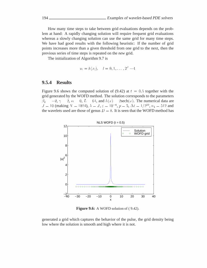
194 Examples of wavelet-based PDE solvers
How many time steps to take between grid evaluations depends on the prob-lem at hand: A rapidly changing solution will require frequent grid evaluationswhereas a slowly changing solution can use the same grid for many time steps.We have had good results with the following heuristic: If the number of gridpoints increases more than a given threshold from one grid to the next, then theprevious series of time steps is repeated on the new grid.
The initialization of Algorithm 9.7 is
ul � h�xl�� l � �� �� � � � � �J � �
9.5.4 Results
Figure 9.6 shows the computed solution of (9.42) at t � ��� together with thegrid generated by the WOFD method. The solution corresponds to the parameters�� � ��, � �, � � �, L � ��, and h�x� � �sech�x�. The numerical data areJ � �� (making N � ����), � � J , � � ����, p � �, �t � �����, n� � ��� andthe wavelets used are those of genus D � �. It is seen that the WOFD method has
−40 −30 −20 −10 0 10 20 30 40−2
0
2
4
6
8
10
12NLS WOFD (t = 0.5)
x
|u|2
Solution WOFD grid
Figure 9.6: A WOFD solution of ( 9.42).
generated a grid which captures the behavior of the pulse, the grid density beinglow where the solution is smooth and high where it is not.

9.5 Wavelet Optimized Finite Difference method 195
Mflops CPU (s) E��u� pointsWOFD�� � ����� ��� �� � ���� � ���WOFD�� � �� ��� ��� � ����FFT split-step ��� �� � ����
Table 9.12: The performance of the WOFD method compared to that of the FFT split-step. The test problem is (9.42) and the numerical data are D � �, � � J � ��,� � t � �� , p � , �t � ����� and � � ����.
Let u� be the result of Algorithm 9.7 using � as threshold and define the compres-sion error
E� �''u� � u�
''�
where the vector u� (� � �) corresponds to the solution obtained using finite dif-ferences on the finest grid. For comparison, we have also implemented the FFT 1
split-step method defined in Section 9.3.4 in Matlab. Table 9.12 shows the num-ber of Mflops (measured in Matlab) needed for each method, the correspondingexecution time, and the compression error E� where applicable. It is seen that theflop count is reduced significantly by the WOFD method but the CPU time is lessso. The latter behavior is probably due to inefficient memory references in theupdating of the finite difference matrices. However, this experiment suggests thatthe WOFD method is potentially very efficient for this problem.
The Matlab functions nlswofd and nlsfft demonstrate the WOFD methodand the FFT split-step method, respectively.
9.5.5 Burgers’ equation revisited
We now illustrate the adaptivity of WOFD by considering a problem where agradient can grow and move with time. The problem concerns Burgers’ equationas given in (9.34).
To test Algorithm 9.7 on (9.34) we have chosen the values � � �����, � �,h�x� � sin���x�. The numerical data are J � ��, � � J , � � ��� , p � �,�t � ����, n� � ��� and D � �. Figure 9.7 show the evolution of u together
1The FFT in Matlab does not precompute the exponentials. Hence it is not as efficient as alibrary FFT.

196 Examples of wavelet-based PDE solvers
0 0.2 0.4 0.6 0.8 10
0.2
0.4
0.6
0.8
1Grid modifications
Pts added
Pts removed
0 0.2 0.4 0.6 0.8 1−1
−0.5
0
0.5
1Burgers’ equation (t = 0.0625)
x
u
Solution
WOFD grid
0 0.2 0.4 0.6 0.8 10
0.2
0.4
0.6
0.8
1Grid modifications
Pts added
Pts removed
0 0.2 0.4 0.6 0.8 1−1
−0.5
0
0.5
1Burgers’ equation (t = 0.25)
x
u
Solution
WOFD grid
0 0.2 0.4 0.6 0.8 10
0.2
0.4
0.6
0.8
1Grid modifications
Pts added
Pts removed
0 0.2 0.4 0.6 0.8 1−1
−0.5
0
0.5
1Burgers’ equation (t = 0.4375)
x
u
Solution
WOFD grid
Figure 9.7: Solution of (9.34) with � � ����� and � � � shown together with theWOFD grid at times t � ����� � ��� � ���� . The numerical data are J � ��, � � J ,� � ��� , p � , �t � ����, and D � �. The lower graphs indicate points that havebeen added (+) and points that have been removed (�) at time t.
with the WOFD grid for different values of t. It is seen that points concentratearound the large gradient as it forms and that the grid becomes very sparse wherethe solution is smooth. Table 9.13 shows the number of Mflops (measured inMatlab) used for � � � and � � ��� .
Finally, Figure 9.9 shows the solution to (9.34) at t � ��� with the sameparameters as before except that we have now introduced linear advection cor-responding to the parameter � ����. It is seen that the WOFD method hascaptured the shock also in this case.
Mflops CPU (s) E��u� pointsWOFD�� � ��� � �� ��� � ���� � ���WOFD�� � �� �� ��� � ����
Table 9.13: The performance of the WOFD method. The test problem is (9.34) with� � ����� and � � � and the numerical data are D � �, � � J � ��, � � t � �� ,p � , �t � ����, and � � ��� .
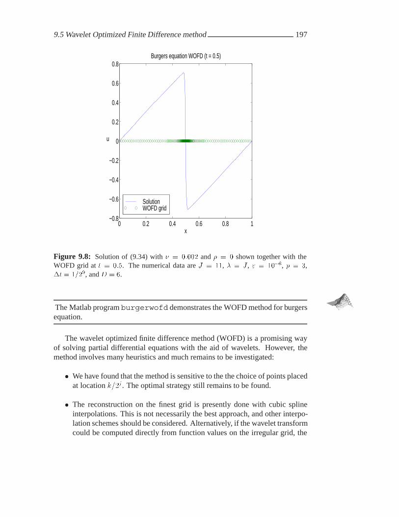
9.5 Wavelet Optimized Finite Difference method 197
0 0.2 0.4 0.6 0.8 1−0.8
−0.6
−0.4
−0.2
0
0.2
0.4
0.6
0.8Burgers equation WOFD (t = 0.5)
x
u
Solution WOFD grid
Figure 9.8: Solution of (9.34) with � � ����� and � � � shown together with theWOFD grid at t � �� . The numerical data are J � ��, � � J , � � ��� , p � ,�t � ����, and D � �.
The Matlab program burgerwofd demonstrates the WOFD method for burgersequation.
The wavelet optimized finite difference method (WOFD) is a promising wayof solving partial differential equations with the aid of wavelets. However, themethod involves many heuristics and much remains to be investigated:
� We have found that the method is sensitive to the the choice of points placedat location k��j . The optimal strategy still remains to be found.
� The reconstruction on the finest grid is presently done with cubic splineinterpolations. This is not necessarily the best approach, and other interpo-lation schemes should be considered. Alternatively, if the wavelet transformcould be computed directly from function values on the irregular grid, the

198 Examples of wavelet-based PDE solvers
0 0.2 0.4 0.6 0.8 1−0.8
−0.6
−0.4
−0.2
0
0.2
0.4
0.6
0.8Burgers equation WOFD (t = 0.5)
x
u
Solution WOFD grid
Figure 9.9: Solution of (9.34) with � � ����� and � � ��� shown together with theWOFD grid at t � �� . The numerical data are J � ��, � � J , � � ��� , p � ,�t � ����, and D � �. The grid points cluster around gradient which has moved fromx � �� to x � ���.
reconstruction could be avoided altogether. Research towards this end is inprogress [Swe96].
� As mentioned earlier, the number of time steps between consecutive gridevaluations should be determined adaptively based on the speed with whichthe solution evolves. Also this point needs further investigation.

Chapter 10
Conclusion
In part � we exposed the theory for compactly supported orthogonal wavelets andtheir periodized forms and gave estimates of their approximation characteristics.Furthermore, we demonstrated that the fast wavelet transform is a viable alterna-tive to the fast Fourier transform whenever one encounters transient phenomenain functions or, as Gilbert Strang [SN96] puts it, wavelets are best for piecewisesmooth functions.
In part 2 we showed how one can implement the fast wavelet transform effi-ciently on a vector computer as well as on parallel architectures. The reason whythe wavelet transform lends itself well to parallelization is a consequence of thelocality of wavelets. Hence, little communication is required. We observed verygood actual performance on the Fujitsu VPP300 as well as the IBM PS2 and it wasshown that our parallel algorithm is optimal in the sense that the scaled efficiencyis independent of the number of processors and it approaches one as the problemsize is increased.
In part 3 we developed several wavelet-based algorithms for solving partialdifferential equations. We derived wavelet differentiation matrices and showedhow one can compute the wavelet transform of a circulant N � N matrix A inO�N� steps using storage bounded by ��N elements. Further, it was shown thatif A is also banded, which is the case for a differentiation matrix, then the workneeded for computing a matrix-vector product in the wavelet domain is O�N�.Moreover, it was shown that the complexity grows with the transform depth �.However, the wavelet compression potential grows with � too. Consequently, thefeasibility of performing such a multiplication depends on whether the gain fromwavelet compression outweighs the increased cost of doing the multiplication inthe wavelet domain. This is the central question for wavelet-based solvers.
200 Conclusion
Examples of the numerical solution of partial differential equations were given.In particular, we developed a wavelet split-step method for the nonlinear Schro-dinger equation as well as Burgers’ equation.
It was observed that the problem size as well as the compression potential mustbe very large for this method to be competitive with traditional methods. Whereasit is straightforward to obtain the wavelet expansion of a known function, it canbe exceedingly difficult to efficiently obtain the wavelet coefficients of a solutionto a partial differential equation. Similar conclusions were reached by [Wal96, p.III-29, V-1], [FS97, Jam94, VP96, CP96, PW96].
Finally, we outlined a different approach called the wavelet optimized finitedifference method. This method uses the wavelet transform as a means for gen-erating an adaptive grid for a traditional finite difference method, and the resultsfor the nonlinear Schrodinger equation and Burgers’ equation are promising. Thepertinent question is not whether an adaptive grid is better than a fixed grid, butwhether it can be generated better and more cheaply through other means thanwavelets. However, this example indicates that wavelets can play the role as apowerful tool for dynamic analysis of the solution as it evolves.
In both cases we observed that the problem size has to be very large and thesolution must be extremely sparse in a wavelet basis before wavelet-based meth-ods for solving partial differential equations have a chance to outperform classicalmethods – and even then, the advantage relies on appropriate choices of severalcritical parameters.
We conclude by pointing out what we see as the main obstacles for obtainingtruly feasible and competitive wavelet-based solvers for partial differential equa-tions. Part of the problem is the fact that there is always a finest level or gridinherent all wavelet approaches. Future research could be directed at methods foravoiding the computations in the space of scaling function or on the finest grid.This would for example require a wavelet transform of data that are not equallyspaced.
Another intrinsic problem is that compression errors tend to accumulate whenapplied to an iterative process. This puts a severe restriction on the amount of ad-missible compression. An error which is acceptable for a compressed signal maybe detrimental for a solution to a partial differential equation when accumulated.Also, when errors are introduced, the solution may become less smooth which inturn means that the subsequent wavelet compression potential drops.
Finally, many algebraic operations in the wavelet domain tend to require com-plicated data structures [BK97, Hol97]. Such data structures may involve pointersand other types of indirect addressing as well as short vectors. For this reasonimplementations are unlikely to perform well on computer architectures such asvector processors.

201
Much research in this field is on its way and it is too early to say whether theproblems mentioned above will be solved. However, there is no doubt that waveletanalysis has earned its place as an important alternative to Fourier analysis — onlythe scope of applicability remains to be settled.


Appendix A
Moments of scaling functions
Consider the problem of computing the moments as given in (2.26):
Mpl �
Z �
��xp��x� l� dx� l� p � Z (A.1)
By the normalization (2.2) we note first that
M�l � �� l � Z (A.2)
Let l � �. The dilation equation (2.17) then yields
Mp� �
Z �
��xp��x� dx
�p�
D��Xk��
ak
Z �
��xp���x� k� dx
�
p�
�p��
D��Xk��
ak
Z �
��yp��y � k� dy� y � �x
or
Mp� �
p�
�p��
D��Xk��
akMpk (A.3)
To reduce the number of unknowns in (A.3) we will eliminate Mpk for k �� �.
Using the variable transformation y � x � l in (A.1) and following a similarapproach as in the derivation on page 20 yields
Mpl �
Z �
���y � l�p��y� dy
�
pXn��
p
n
lp�n
Z �
��yn��y� dy
204 Moments of scaling functions
or
Mpl �
pXn��
p
n
lp�nMn
� (A.4)
Substituting (A.4) into (A.3) we obtain
Mp� �
p�
�p��
D��Xk��
ak
pXn��
p
n
kp�nMn
�
�
p�
�p��
p��Xn��
p
n
Mn
�
D��Xk��
akkp�n �
p�
�p��Mp
�
D��Xk��
ak� �z �p�
Solving for MP� yields
Mp� �
p�
���p � ��
p��Xn��
p
n
Mn
�
D��Xk��
akkp�n (A.5)
Equation (A.5) can now be used to determine the pth moment of ��x�, Mp� for
any p � �. For p � � use (A.2). The translated moments Mpl are then obtained
from (A.4).
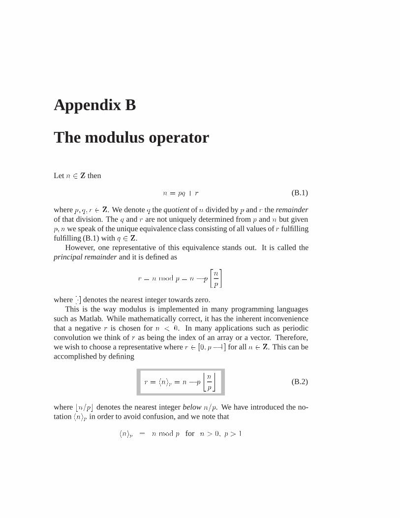
Appendix B
The modulus operator
Let n � Z then
n � pq � r (B.1)
where p� q� r � Z. We denote q the quotient of n divided by p and r the remainderof that division. The q and r are not uniquely determined from p and n but givenp� nwe speak of the unique equivalence class consisting of all values of r fulfillingfulfilling (B.1) with q � Z.
However, one representative of this equivalence stands out. It is called theprincipal remainder and it is defined as
r � n mod p � n � p
�n
p
�
where �� denotes the nearest integer towards zero.This is the way modulus is implemented in many programming languages
such as Matlab. While mathematically correct, it has the inherent inconveniencethat a negative r is chosen for n � �. In many applications such as periodicconvolution we think of r as being the index of an array or a vector. Therefore,we wish to choose a representative where r � �� p� �� for all n � Z. This can beaccomplished by defining
r � hnip � n� p
n
p
!(B.2)
where bn�pc denotes the nearest integer below n�p. We have introduced the no-tation hnip in order to avoid confusion, and we note that
hnip � n mod p for n � �� p � �

206 The modulus operator
For practical purposes hnip should not be implemented as in (B.2); rather, itshould be written using the built-in modulus function modifying the result when-ever needed.
The programming language Fortran 90 includes both definitions, so MOD(n,p)is the ordinary modulus operator, where MODULO(n,p) implements hnip (see[MR96, p 177]).
Definition B.1 Let n be given as in (B.1). If r � �, we say that p is a divisor in nand write
p j n
It follows that for all p� q� n� r � Z we have
p j �n � r� and q j �n� r�
Lemma B.1 Let n�� n�� q � Z. Then
hn� � n�iq � hn� � hn�iqiqhn�n�iq � hn�hn�iqiq
Proof: We write n� as in (B.1) and find
hn� � n�iq � hn� � �p�q � r��iq� hn� � r�iq� hn� � hn�iqiq
and
hn�n�iq � hn��p�q � r��iq� hn�p�q � n�r�iq� hn�r�iq� hn�hn�iqiq
�

207
Lemma B.2 Let k� n� q � Z. Then
khniq � hknikq
Proof: We write n as in (B.1). Then
q j �n� r�
for q� n� r � Z. When q is a divisor in n� r then also
kq j k�n� r�
from which we get
kr � hknikq�

208 The modulus operator

Appendix C
Circulant matrices and the DFT
We state some properties of circulant matrices and describe their relation to con-volution and the discrete Fourier transform (DFT).
Definition C.1 (Circulant matrix) Let A be an N � N matrix and let a �a�� a�� � � � � aN���T be the first column of A. ThenA is circulant if
A�m�n � ahm�niN � m� n � �� �� � � � � N � �
A circulant �� � matrix has the form"BB#
a� a� a� a�a� a� a� a�a� a� a� a�a� a� a� a�
$CCA
Since all columns are shifted versions of a, it suffices to store the N elements ofa instead of the N� elements of A. Also, computational work can be saved usingthe circulant structure.
Matrix vector multiplication with a circulant matrix is closely related to dis-crete (cyclic) convolution which is defined as follows
Definition C.2 (Discrete convolution) Let x � x�� x�� � � � � xN���T and definey and z similarly. Then
z � x � yis the (cyclic) convolution defined by
zm �
N��Xn��
xnyhm�niN � m � �� �� � � � � N � � (C.1)

210 Circulant matrices and the DFT
The discrete Fourier transform (DFT) is closely related to convolution and circu-lant matrices. We define it as follows:
Definition C.3 (Discrete Fourier transform) Let fxlgN��l�� be a sequence of Ncomplex numbers. The sequence fxkgN��k�� defined by
xk �N��Xl��
xl��klN � k � �� �� � � � � N � �
where �N � ei���N , is the discrete Fourier transform of fxlgN��l�� .
There are a number of variants of the DFT in the literature, and no single defini-tion has a clear advantage over the others. A particular variant should therefore bechosen such that it suits the context best. The choice we have made here is mainlymotivated by the fact that it yields a simple form of the convolution theorem (The-orem C.1).
Let x � x�� x�� � � � � xN���T and x � x�� x�� � � � � xN���T . Then the DFT canbe written in matrix-vector form as
x � FNx (C.2)
where
FN �k�l � ��klN � e�i��kl�N (C.3)
is the N �N Fourier matrix.The inverse of FN satisfies the relation
F��N �
�
NFN (C.4)
This is seen from the matrix product
FN �m�kFN �k�n �
N��Xk��
�k�n�m�N �
�N m � n� m �� n
Consequently, x � F��N x and we have
Definition C.4 (Inverse discrete Fourier transform) Let fxlgN��l�� and fxkgN��k��
be given as in Definition C.3. Then the inverse discrete Fourier transform (IDFT)is defined as
xl ��
N
N��Xk��
xk�klN � l � �� �� � � � � N � � (C.5)

211
Both the DFT and the IDFT can be computed inO�N log�N� steps using the fastFourier transform algorithm (FFT).
The link between DFT and convolution is embodied in the convolution theo-rem, which we state as follows:
Theorem C.1 (Convolution theorem)
z � x � y z � diag�x�y
Proof: We begin by writing the components of x and y in terms of those of x andy, i.e.
xn ��
N
N��Xk��
xk�knN
yhm�niN ��
N
N��Xk��
yk�khm�niNN �
�
N
N��Xk��
�yk��knN ��km
N
since exp�i��hniN�N� � exp�i��n�N�. Consequently,
zm �N��Xn��
��
N
N��Xk��
xk�knN �
�
N
N��Xl��
yl��lnN �lm
N
��
N�
N��Xk��
N��Xl��
xkyl�lmN
N��Xn��
�n�k�l�N
��
N
N��Xk��
xkyk�kmN
Hence zk � xkyk for k � �� �� � � � � N � � by the definition of the IDFT (C.5). �
Corollary C.2 The convolution operator is commutative
x � y � y � xProof: Using Theorem C.1 we get
x � y � F��N diag�x�y � F��
N diag�y�x � y � x�

212 Circulant matrices and the DFT
Matrix multiplication with a circulant matrix is equivalent to a convolution:
Lemma C.3 LetA and a be defined as in Definition C.1 and x � RN then
Ax � a � x
Proof:
Ax�m �N��Xn��
A�m�nxn �N��Xn��
ahm�niNxn
� x � a�m � a � x�m� m � �� �� � � � � N � �
�
We now use the convolution theorem to obtain an alternative and useful charac-terization of circulant matrices.
Theorem C.4
A is circulant A � F��N �aFN � �a � diag�a�
Proof:
�: Let A be an N �N circulant matrix and let x and y be arbitrary vectors oflength N . Then, by Lemma C.3 and Theorem C.1
y � Ax
� a � x� F��
N diag�a�x
� F��N diag�a�F Nx
the factorization follows.
�: Let A � F��N �aFN and let en � I ��n be the n’th unit vector of length N .
The element A�m�n can then be extracted as follows
A�m�n � F��N �aF N �m�n
��
NeTmFN
T�aFNen
��
N
N��Xk��
�kmN ak�
�knN
��
N
N��Xk��
ak�k�m�n�N
� ahm�niN
Hence A is circulant according to Definition C.1.
�

213
Theorem C.5 Circulant matrices with the same dimensions commute.
Proof: Let A and B be circulant N � N matrices according to Definition C.1.Then we have from Theorem C.4
AB � F��N �aF NF
��N �bFN � F��
N �a�bFN
Since �a and �b are diagonal, they commute and we find
AB � F��N �b�aFN � F��
N �bFNF��N �aF N � BA
�
Theorem C.6
A is circulant A�� is circulant
with
A�� � F��N ���
a FN � �a � diag�a�
Proof: Using the factorization given in Theorem C.4 we find
A�� � �F��N �aFN�
�� � F��N ���
a FN
�
Since �a is diagonal, ���a is computed in N operations. Hence the computa-
tional complexity of computing A�� is dominated by that of the FFT which isO�N log�N�.

214 Circulant matrices and the DFT

Appendix D
Fourier differentiation matrix
Let f be a � periodic function which is d times differentiable and consider itsFourier expansion
f�x� ��X
k���cke
i��kx� x � R (D.1)
where ck �R �
� f�x�e�i��kx dx.
We approximate f by the truncated expansion
fN�x� �
N����Xk��N��
ckei��kx� x � R
Differentiating d times then yields
f�d�N �x� �
N����Xk��N��
c�d�k ei��kx� x � R
where
c�d�k � �i��k�dck� k � �N
���N
�� �� � � � �
N
�� �
Hence f �d�N �x� approximates f �d��x�.Let N � �J for J � N and xl � l�N , l � �N����N�� � �� � � � � N�� � �.
Define the vectors f and f �d� as
fl � fN �xl� �
N����Xk��N��
ckei��kxl �
N����Xk��N��
ck�klN (D.2)
f�d�l � f
�d�N �xl� �
N����Xk��N��
c�d�k ei��kxl �
N����Xk��N��
c�d�k �kl
N (D.3)
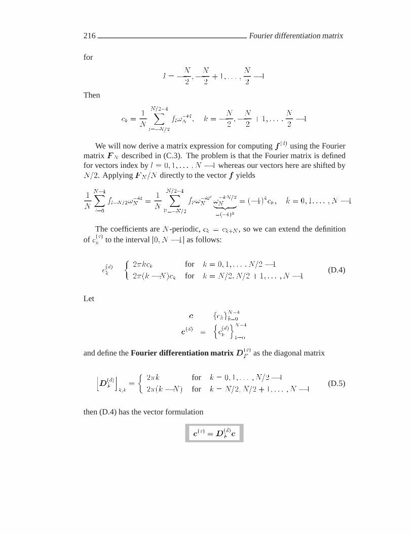
216 Fourier differentiation matrix
for
l � �N
���N
�� �� � � � �
N
�� �
Then
ck ��
N
N����Xl��N��
fl��klN � k � �N
���N
�� �� � � � �
N
�� �
We will now derive a matrix expression for computing f �d� using the Fouriermatrix F N described in (C.3). The problem is that the Fourier matrix is definedfor vectors index by l � �� �� � � � � N � � whereas our vectors here are shifted byN��. Applying F N�N directly to the vector f yields
�
N
N��Xl��
fl�N����klN ��
N
N����Xl���N��
fl���kl�N �
�kN��N� �z ������k
� ����kck� k � �� �� � � � � N � �
The coefficients are N -periodic, ck � ck�N , so we can extend the definitionof c�d�k to the interval �� N � �� as follows:
c�d�k �
���kck for k � �� �� � � � � N�� � �
���k �N�ck for k � N��� N�� � �� � � � � N � �(D.4)
Let
c � fckgN��k��
c�d� �nc�d�k
oN��
k��
and define the Fourier differentiation matrixD�d�F as the diagonal matrix
hD
�d�F
ik�k
�
���k for k � �� �� � � � � N��� �
���k �N� for k � N��� N�� � �� � � � � N � �(D.5)
then (D.4) has the vector formulation
c�d� �D�d�F c

217
Applying NF ��N to c�d� then yields
N��Xk��
����kc�d�k �klN �
N��Xk��
c�d�k �kl
N��kN��N
�N��Xk��
c�d�k �
k�l�N���N
� f�d�l�N��� l � �� �� � � � � N � �
Hence N and ��N cancel out and we arrive at
f �d� � F��N D
�d�F F Nf
The shift in (D.5) can for example be done in Matlab using FFTSHIFT or asimilar function. If the period is different from �, say L, then D�d�
F must be scaledas described in Section 7.4.1.

218 Fourier differentiation matrix

Appendix E
List of Matlab programs
The following Matlab programs demonstrate selected algorithms and are availableon the World Wide Web at
http://www.imm.dtu.dk/˜omni/wapa20.tgz
More documentation is found in the enclosed README file.
Function Page Descriptionwavecompare 10 Compares a wavelet approximation to a
Fourier approximationbasisdemo 10 Generates and displays periodic waveletsdaubfilt 16 Returns a vector containing the filter coeffi-
cients a�� a�� � � � � aD��low2hi 17 Computes fbkgD��k�� from fakgD��k��
filttest 21 Checks vector of filter coefficientscascade 45 Computes function values for ��x� and ��x�dst, idst 49 Computes the DST and its inversefwt, ifwt 59 Computes the FWT and its inversefwt2, ifwt2 60 Computes the 2D FWT and its inverseconn 111 Computes �d for a given wavelet genus Ddiftest 117 Tests convergence rates for D�d� and Dd
difmatrix 118 Computes the differentiation matrixD�d��Ld
nlsfft 195 Demonstrates the FFT split-step method forthe Nonlinear Schrodinger equation
nlswofd 195 Demonstrates the WOFD method for thenonlinear Schrodinger equation
burgerwofd 197 Demonstrates the WOFD method for Burg-ers’ equation


Bibliography
[AB84] O. Axelsson and V. A. Barker. Finite Element Solution of BoundaryValue Problems. Computer Science and Applied Mathematics. Aca-demic Press, 1984.
[Agr89] G. P. Agrawal. Nonlinear Fiber Optics. Academic Press, 1989.
[Bar96] V. A. Barker. Computing connection coefficients. Technical ReportIMM-REP-1996-5, Technical University of Denmark, 1996.
[BCR91] G. Beylkin, R. Coifman, and V. Rohklin. Fast wavelet transforms andnumerical algorithms. Comm. Pure Appl. Math., 44:141–183, 1991.
[Bey92] G. Beylkin. On the representation of operators in bases of compactlysupported wavelets. SIAM J. Num. Anal., 29(6):1716–1740, 1992.
[Bey93] G. Beylkin. Wavelets and fast numerical algorithms. In Different Per-spectives on Wavelets, pages 89–117. AMS, 1993.
[Bey94] G. Beylkin. On wavelet-based algorithms for solving differential equa-tions”,. In J. J. Benedetto and M. W. Frazier, editors, Wavelets - Mathe-matics and Applications, chapter 12, pages 449–466. CRC Press, 1994.
[BK97] G. Beylkin and J. M. Keiser. On the adaptive numerical solution of non-linear partial differential equations in wavelet bases. J. Comp. Phys.,132:233–259, 1997.
[BMP90] E. Bacry, S. Mallat, and G. Papanicolaou. A wavelet based space-timeadaptive numerical method for partial differential equations. Technicalreport, Courant Institute of Mathematical Sciences, New York, 1990.
[BN96] S. Bertoluzza and G. Naldi. A wavelet collocation method for the nu-merical solution of partial differential equations. Appl. Comp. Har-monic Anal., 3:1–9, 1996.
221

222 Bibliography
[Cha96] P. Charton. Produits de matrices rapides en bases d’ondelettes: ap-plication a la resolution numerique d’equations aux derives partielles.PhD thesis, Universite de Paris Nord, 1996.
[Chu97] C. K. Chui. Wavelets: A Mathematical Tool for Signal Analysis. SIAM,1997.
[CP96] P. Charton and V. Perrier. A pseudo-wavelet scheme for the two-dimensional Navier-Stokes equations. Matematica Aplicada e Com-putational, 15(2):139–160, 1996.
[Dau88] I. Daubechies. Orthonormal bases of compactly supported wavelets.Comm. Pure Appl. Math., XLI(7):909–996, 1988.
[Dau92] I. Daubechies. Ten Lectures on Wavelets. SIAM, 1992.
[DKU96] W. Dahmen, A. Kunoth, and K. Urban. A wavelet Galerkin method forthe Stokes equations. Computing, 56:259–301, 1996.
[DMC95] B. K. Das, R. N. Mahapatra, and B. N. Chatterli. Modelling of wavelettransform on multistage interconnection network. In Proceedings ofthe Australasian Conference on Parallel and Real-Time Systems, pages134–142, Freemantle, Western Australia, 28-29 September 1995.
[Dor95] M. Dorobantu. Wavelet-based Algorithms for Fast PDE Solvers. PhDthesis, Royal Institue of Technology, Stockholm, 1995.
[EBR97] L. Elden, F. Berntsson, and T. Reginska. Wavelet and Fourier meth-ods for solving the sideways heat equation. Preprint. Department ofMathematics, Linkobing University, 1997.
[Eir92] T. Eirola. Sobolev characterization of solutions of dilation equations.SIAM J. Math. Anal., 23(4):1015–1030, 1992.
[EL] F. Ekstedt and M. Lindberg. Diagonalization of homogeneous linearoperators in biorthogonal wavelet bases.ftp.math.chalmers.se/pub/users/mlind/diag.a4.ps.gz.
[EOZ94] B. Engquist, S. Osher, and S. Zhong. Fast wavelet based algorithms forlinear evolution equations. SIAM J. Sci. Comp., 15(4):755–775, 1994.
[F�96] M. Farge et al. Wavelets and turbulence. Proc. IEEE, 84(4):639–669,1996.
223
[FJAF78] M. D. Feit and Jr J. A. Fleck. Light propagation in graded-index opticalfibers. Appl. Optics, 17(24):3990–3998, 1978.
[Fol95] G. B. Folland. Introduction to Partial Differential Equations. PrincetonUniversity Press, 1995.
[FS97] J. Frolich and K. Schneider. An adaptive wavelet-vaguelette algorithmfor the solution of pdes. J. Comp. Phys., 130(2):174–190, 1997.
[GL89] G. H. Golub and C. Van Loan. Matrix Computations. John HopkinsUniversity Press, 2 edition, 1989.
[GL94] L. Gagnon and J. M. Lina. Symmetric daubechies’ wavelets and nu-merical solution of nls equations. J. Phys. A: Math Gen, 27:8207–8230,1994.
[H�94] C. Hsiao et al. Near optimal compression of orthonormal wavelet ex-pansions. In J. J. Benedetto and M. W. Frazier, editors, Wavelets -Mathematics and Applications, chapter 11, pages 425–446. CRC Press,1994.
[Heg95] M. Hegland. An implementation of multiple and multi-variate fastFourier transforms on vector processors. SIAM J. Sci. Comp.,16(2):271–288, 1995.
[Heg96] M. Hegland. Real and complex fast Fourier transforms on the Fu-jitsu VPP500. Parallel Comp., 22:539–553, 1996.
[HJ88] R. W. Hockney and C. R. Jesshope. Parallel Computers 2. IOP Pub-lishing Ltd, 1988.
[Hol97] M. Holmstrom. Wavelet Based Methods for Time Dependent PDEs.PhD thesis, Department of Scientific Computing, Uppsala University,1997.
[HPW94] F. Heurtaux, F. Planchon, and Mladen Victor Wickerhauser. Scale de-composition in burgers’ equation. In J. J. Benedetto and M. W. Frazier,editors, Wavelets - Mathematics and Applications, chapter 14, pages505–523. CRC Press, 1994.
[HW96] E. Hernandez and G. Weiss. A First Course on Wavelets. CRC Press,1996.
[Jam93] L. Jameson. On the Daubechies-based wavelet differentiation matrix.J. Sci. Comp., 8(3):267–305, 1993.

224 Bibliography
[Jam94] L. Jameson. On the wavelet-optimized finite difference method. Tech-nical Report NASA CR-191601, ICASE Report No. 94-9, 1994.
[Jam96] L. Jameson. The wavelet-optimized finite difference method. In G. Er-lebacher and M. Y. Hussaini an L. Jameson, editors, Wavelets. Theoryand Applications, chapter 1.5, pages 16–22. Oxford University Press,1996.
[JS93] B. Jawerth and W. Sweldens. Wavelet resolution analysis adapted forthe fast solution of boundary value ordinary differential equations. InProceedings of the sixth Copper Mountain Multigrid Conference, 1993.
[JS94] B. Jawerth and W. Sweldens. An overview of wavelet based multires-olution analysis. SIAM Review, 36(3):377–412, 1994.
[Kai94] G. Kaiser. A Friendly Guide to Wavelets. Birkhauser, 94.
[Kei95] J. M. Keiser. Wavelet Based Approach to Numerical Solution of Nonlin-ear Partial Differential Equations. PhD thesis, University of Colorado,1995.
[Kun94] A. Kunoth. Computing integrals of refinable functions - documentationof the program. Technical report, SINTEF, 1994.
[LBA81] M. Lax, J.H. Batteh, and G.P. Agrawal. Channeling of intense electro-magnetic beams. J. Appl. Phys., 52(1):109–125, 1981.
[LPT92] J. Liandrat, V. Perrier, and P. H. Tchamitchan. Numerical resolutionof nonlinear partial differential equations using the wavelet approach.In Mary Beth Ruskai et al., editors, Wavelets and their applications,pages 227–238. Jones and Bartlett, 1992.
[LR94] G. Leaf and J. M. Restrepo. Wavelet-Galerkin discretization of hyper-bolic equations. Technical report, Argonne National Laboratory, USA,1994.
[LRT91] A. Latto, H. L. Resnikoff, and E. Tenenbaum. The evaluation of con-nection coefficients of compactly supported wavelets. Technical re-port, AWARE, Inc, One Memorial Drive, Cambridge, MA 02142-1301,USA, 1991.
[LS95] R. Lang and A. Spray. The 2D wavelet transform on a massively paral-lel machine. In Proceedings of the Australasian Conference on Paral-lel and Real-Time Systems, pages 325–332, Freemantle, Western Aus-tralia, 28-29 September 1995 1995.

225
[LT90a] A. Latto and E. Tenenbaum. Compactly supported wavelets and thenumerical solution of burgers’ equation. C.R. Acad. Sci. Paris, t. 311,Serie I, pages 903–909, 1990.
[LT90b] J. Liandrat and P. Tchamitchian. Resolution of the 1D regularized burg-ers equation using spatial wavelet approximation. Technical Report90-83, ICASE, 1990.
[Lu93] J. Lu. Parallelizing mallat algorithm for 2-D wavelet transforms. Inf.Proc. Letters, 45:255–259, 1993.
[Mal89] S. G. Mallat. A theory for multiresolution signal decomposition: Thewavelet representation. IEEE Trans. PAMI, 11(7):674–693, 1989.
[Mey93] Y. Meyer. Wavelets: Algorithms and Applications. SIAM, 1993.
[MR96] M. Metcalf and J. Reid. Fortran 90/95 explained. Oxford SciencePublications, 1996.
[New92] A. C. Newell. Nonlinear Optics. Addison-Wesley, 1992.
[New93] D. E. Newland. Random Vibrations, Spectral & Wavelet Analysis.Longman Scientific & Technical, 1993.
[NH95] O. M. Nielsen and M. Hegland. Two-dimensional fast wavelet trans-form on the VP2200. Semi-annual report on the Fujitsu-ANU parallelmathematical subroutine library project, Australian National Univer-sity, 1995.
[NH97] O. M. Nielsen and M. Hegland. A scalable parallel 2D wavelet trans-form algorithm. ANU Computer Science Technical Reports TR-CS-97-21, Australian National University, 1997. Submitted to ParallelComputing.
[Nie97] O. M. Nielsen. Fast 2D wavelet transform of circulant matrices. Tech-nical Report IMM-REP-1997-8, Technical University of Denmark,1997.
[PAP86] M. J. Potasek, G. P. Agrawal, and S. C. Pinault. Analytic and numericalstudy of pulse broadening in nonlinear dispersive optical fivbers. J.Opt. Soc. Am. B, 3(2):205–211, 1986.
[PB91] V. Perrier and C. Basdevant. Travelling wavelets method. In Proc. ofthe US-French ’Wavelets and Turbulence’ Workshop. Princeton, 1991.

226 Bibliography
[PK91] D. Pathria and G. Karniadakis. Wavelet-aided spectral element flowsimulations. Preprint Princeton, 1991.
[PW96] I. Pierce and L. Watkins. Modelling optical pulse propagation in non-linear media using wavelets. Technical report, School of ElectronicEngineering and Computer Systems, University of Wales, Bangor, UK,1996.
[QW93] S. Quian and J. Weiss. Wavelets and the numerical solution of partialdifferential equations. J. comp. phys., 106:155–175, 1993.
[RE97] T. Reginska and L. Elden. Solving the sideways heat equation by awavelet-Galerkin method. Inv. Prob., 13:1093–1106, 1997.
[Smi85] G.D. Smith. Numerical Solution of Partial Differential Equations: Fi-nite Difference Methods. Oxford University Press, 1985.
[SN96] G. Strang and T. Nguyen. Wavelets and Filter Banks. Wellesley-Cambridge Press, 1996.
[Spi93] M. R. Spiegel. Mathematical Handbook of Formulas and Tables.Schaum’s Outline Series, 1993.
[Str92] G. Strang. Wavelet transforms versus Fourier transforms. Technicalreport, MIT, Department of Mathematics, MIT, Cambridge MA 02139,1992.
[Str94] R. S. Stricharz. Construction of orthonormal wavelets. In John J.Benedetto and Michael W. Frazier, editors, Wavelets - Mathematicsand Applications, chapter 1, pages 23–51. CRC Press, 1994.
[Str96] G. Strang. Creating and comparing wavelets. Available from the author([email protected]), 1996.
[Swe] W. Sweldens. Wavelet resources. Available athttp://www.mathsoft.com/wavelets.html.
[Swe96] W. Sweldens. Wavelets: What next ? Proc. IEEE, 84(4):680–685,1996.
[Uni96] Australian National University. ANU VPP300. Available athttp://anusf.anu.edu.au/VPP/, 1996.
[VK95] M. Vetterli and J. Kovacevic. Wavelets and Subband Coding. PrenticeHall, 1995.

227
[VP96] O. V. Vasilyev and S. Paolucci. A dynamically adaptive multilevelwavelet collocation method for solving partial differential equation ina finite domain. J. comp. phys., 125:498–512, 1996.
[WA94] J. R. Williams and K. Amaratunga. Wavelet-Galerkin solutions forone-dimensional partial differential equations. Int J. Num. Meth. Eng.,37:2703–2716, 1994.
[Wal96] J. Walden. Wavelet Solvers for Hyperbolic PDEs. PhD thesis, Depart-ment of Scientific Computing, Uppsala University, 1996.
[WM85] R. Wait and A. R. Mitchell. Finite Element Analysis and Applications.John Wiley & Sons Ltd., 1985.
[WZ94] L. Watkins and Y. R. Zhou. Modelling propagation in optical fibersusing wavelets. J. Lightwave Tech., 12(9):1536–1542, 1994.
[XS92] J. C. Xu and W. C. Shann. Galerkin-wavelet methods for two pointboundary value problems. In Num. Math. [Swe], pages 123–144.


Index
2D FWT, 60of circulant matrix, 121, 127of circulant, banded matrix, 146parallelization of, 95vector performance, 81
2D circulant wavelet transformalgorithm, 139complexity, 140storage, 142storage requirement, 145
accuracyof the multiresolution spaces, 61of wavelet differentiation matrix,
115of wavelet-Galerkin method, 165
Amdahl’s law, 85approximating scaling function coef-
ficients by scaled function val-ues, 66
approximation properties, 61–70of �VJ , 63of VJ , 61
approximation spaces, 11–13, 38arithmetic-geometric series, 144
banded circulant matrix, 146bandwidth, 114, 116, 146basic scaling function, 13basic wavelet, 13Burgers’ equation, 185, 195
calculation of bandwidths, 147cascade algorithm, 43
CFWT, 97circulant 2D wavelet transform
algorithm, 139complexity of, 140storage, 142storage requirement, 145
circulant matrix, 209and convolution, 212and DFT, 212commutation, 213inverse, 213wavelet transform of, 121, 127
CIRFWT, 139CIRMUL, 158column-shift-circulant matrix, 127communication, 89communication-efficient FWT, 95, 97
performance model for, 97complexity
of 2D circulant wavelet transform,140
of 2D FWT, 60of FWT, 59of matrix-vector multiplication in
the wavelet domain, 159of wavelet split-step method, 182
compression, 64, 67–70error, 69, 173of A��, 171of matrix, 171of solution to Burgers’ equation,
189
229

230 Index
of solution to the nonlinear Schrodingerequation, 178
of vector, 171connection coefficients, 108conservation of area, 33convolution, 209convolution theorem, 211
data structure for 2D wavelet trans-form, 136
depth, 15DFT, 210
and circulant matrices, 212differential equations
examples, 163–198differentiation matrix, 114
convergence rate, 115, 165Fourier, 215with respect to physical space, 115with respect to scaling functions,
114with respect to wavelets, 119WOFD, 190
dilation equation, 15, 16, 33in frequency domain, 25
discrete Fourier transform, 210DST, 49
evaluation of scaling function expan-sions, 47
expansionFourier, 3periodic scaling functions, 39periodic wavelets, 39scaling functions, 14, 47wavelets, 6, 14
fast wavelet transform, 52–60complexity of, 59of circulant matrix, 127of circulant, banded matrix, 146
FFT split-step method, 185
filter coefficients, 16finite differences on an irregular grid,
189Fourier differentiation matrix, 215, 216Fourier expansion, 3Fourier transform
continuous, 25discrete, 210inverse discrete, 210
Fujitsu VPP300, 73, 99FWT, 52, 59, 121
complexity of, 59Definition of, 58Matrix formulation, 56parallelization of, 86periodic, 54vector performance, 74
genus, 16grid generation using wavelets, 193
heat equation, 168hybrid representation, 170with respect to physical space, 169with respect to scaling functions,
168with respect to wavelets, 169
Helmholz equation, 163hybrid representation, 167with respect to physical space, 167with respect to scaling functions,
163with respect to wavelets, 166
IBM SP2, 99IDFT, 210IDST, 49IFWT, 54, 59
periodic, 56Ij�l, 17inverse discrete Fourier transform, 210inverse fast wavelet transform, 54
231
inverse partial wavelet transform, 54IPWT, 54
periodic, 56
Kronecker delta, 14
�, 15
Mallat’s pyramid algorithm, see fastwavelet transform
Matlab programs, 219matrix
banded, 146circulant, 209column-shift-circulant, 127row-shift-circulant, 127
matrix exponential of a circulant ma-trix, 176
matrix-vector multiplication in a waveletbasis, 153, 158
complexity, 159MFWT, 79
parallel algorithm for, 91parallelization of, 91performance model for, 93vectorization of, 79
modulus operator, 205moments
of scaling functions, 203vanishing, 19
motivation, 3multiple 1D FWT, 79multiresolution analysis, 11
nonlinear Schrodinger equation, 174,191
numerical evaluation of � and �, 43
orthogonality, 14, 33in frequency domain, 30
parallel performanceof the 2D FWT, 96–100
of the MFWT, 93parallel transposition and data distri-
bution, 96parallelization, 85
of the 2D FWT, 95of the FWT, 86of the MFWT, 91
Parseval’s equation for wavelets, 15partial differential equations, see dif-
ferential equationspartial wavelet transform, 53PDEs, see differential equationsperformance model
for the communication-efficient FWT,97
for the MFWT, 93for the replicated FWT, 96
periodic boundary value problem, 163periodic functions
on the interval a� b�, 50periodic FWT, 54periodic IFWT, 56periodic initial-value problem, 168, 174,
185periodic IPWT, 56periodic PWT, 54periodic scaling function
expansion, 39periodic wavelet
expansion, 39periodized wavelets, 33�, 13Projection
on �Vj and �Wj , 41on Vj and Wj , 15
projection methods, 107property of vanishing moments, 20�, 13pth moment of ��x� k�, 19PWT, 53
periodic, 54

232 Index
pyramid algorithm, see fast wavelettransform
replicated FWT, 95performance model for, 96
RFWT, 95row-shift-circulant matrix, 127
scale parameter, 6scaling function, 13
expansion, 14, 47evaluation of, 47
in frequency domain, 25moments of, 203periodized, 33support of, 17
shift parameter, 6shift-circulant matrices, 127SP2, 99split-step method, 175
FFT, 185wavelet, 175
split-transpose algorithm, 81storage of 2D circulant wavelet trans-
form, 142storage requirement, 145support, 17survey of wavelet applications to PDEs,
105
time stepping in the wavelet domain,170
two term connection coefficients, 108
VJapproximation properties of, 61definition of, 11
�VJapproximation properties of, 63definition of, 38
vanishing moments, 19, 20, 33vector performance
of the 2D FWT, 81of the FWT, 74
vectorizationof the 2D FWT, 81of the FWT, 73of the MFWT, 79
VPP300, 99
WJ
definition of, 12�WJ
definition of, 38wavelet, 13
algorithms, 43–60basic, 13differentiation matrices, 105–119expansion, 6, 14genus, 16in frequency domain, 25periodized, 33support of, 17
wavelet compression, see compressionwavelet differentiation matrix, 119wavelet equation, 15, 16
in frequency domain, 29wavelet optimized finite difference method,
188wavelet split-step method, 175
complexity of, 182wavelet transform, see fast wavelet trans-
formwavelets
on the real line, 11on the the unit interval, 33
WOFD, see wavelet optimized finitedifference method