arX

iv:c

ond-

mat

/050

6300

v1

14

Jun

2005

Wavepacket Dynamics, Quantum Reversibility andRandom Matrix Theory

Moritz Hiller a,∗, Doron Cohenb, Theo Geisela, Tsampikos Kottosa

aMax-Planck-Institute for Dynamics and Self-OrganizationandDepartment of Physics, University of Gottingen, Bunsenstraße 10, D-37073 Gottingen

bDepartment of Physics, Ben-Gurion University, Beer-Sheva84105, Israel

Abstract

We introduce and analyze the physics of “driving reversal” experiments. These are pro-totype wavepacket dynamics scenarios probing quantum irreversibility. Unlike the mostlyhypothetical “time reversal” concept, a “driving reversal” scenario can be realized in a lab-oratory experiment, and is relevant to the theory of quantumdissipation. We study boththe energy spreading and the survival probability in such experiments. We also introduceand study the ”compensation time” (time of maximum return) in such a scenario. Exten-sive effort is devoted to figuring out the capability of either Linear Response Theory (LRT)or Random Matrix Theory (RMT) in order to describe specific features of the time evolu-tion. We explain that RMT modeling leads to a strong non-perturbative response effect thatdiffers from the semiclassical behavior.

Key words: Quantum Dissipation, Quantum Chaos, Random Matrix TheoryPACS:03.65.-w, 03.65.Sq, 05.45.Mt, 73.23.-b

1 Introduction

In recent years there has been an increasing interest in understanding the theoryof driven quantized chaotic systems [1,2,3,4,5,6,7,8,9,10,11]. Driven systems aredescribed by a HamiltonianH(Q, P, x(t)), wherex(t) is a time dependent param-eter and(Q, P ) are some generalized actions. Due to the time dependence ofx(t),the energy of the system is not a constant of motion. Rather the system makes”transitions” between energy levels, and therefore absorbs energy. This irreversible

∗ Corresponding authorEmail address:mhiller@chaos.gwdg.de (Moritz Hiller).

Preprint submitted to Elsevier Science 15 June 2005

loss of energy is known asdissipation. To have a clear understanding of quantumdissipation we need a theory for the time evolution of the energy distribution.

Unfortunately, our understanding on quantum dynamics of chaotic systems is stillquite limited. The majority of the existing quantum chaos literature concentrates onunderstanding the properties of eigenfunctions and eigenvalues. One of the mainoutcomes of these studies is the conjecture that Random Matrix Theory (RMT)modeling, initiated half a century ago by Wigner [12,13], can capture theuniversalaspects of quantum chaotic systems [14,15]. Due to its largesuccess RMT hasbecome a major theoretical tool in quantum chaos studies [14,15], and it has foundapplications in both nuclear and mesoscopic physics (for a recent review see [16]).However, its applicability to quantum dynamics was left unexplored [17,18].

This paper extends our previous reports [10,17,18] on quantum dynamics, both indetail and depth. Specifically, we analyze two dynamical schemes: The first is theso-called wavepacket dynamics associated with a rectangular pulse of strength+ǫwhich is turned on for a specified duration; The second involves an additional pulsefollowed by the first one which has a strength−ǫ and is of equal duration. We definethis latter scheme asdriving reversalscenario. We illuminate the direct relevance ofour study with the studies of quantum irreversibility of energy spreading [10] andconsequently with quantum dissipation. We investigate theconditions under whichmaximum compensation is succeeded and define the notion of compensation (echo)time. To this end we rely both on numerical calculations performed for a chaoticsystem and on analytical considerations based on Linear Response Theory (LRT).The latter constitutes the leading theoretical framework for the analysis of drivensystems and our study aims to clarify the limitations of LRT due to chaos. Our re-sults are always compared with the outcomes of RMT modeling.We find that theRMT approach fails in general, to give the correct picture ofwave-evolution. RMTcan be trusted only to the extend that it gives trivial results that are implied by per-turbation theory. Non-perturbative effects are sensitiveto the underlying classicaldynamics, and therefore the~ → 0 behavior for effective RMT models is strikinglydifferent from the correct semiclassical limit.

The structure of this paper is as follows: In the next sectionwe discuss the no-tion of irreversibility which is related to driving reversal schemes and distinguishit from micro-reversibility which is associated with time reversal experiments. InSection 3 we discuss the driving schemes that we are using andwe introduce thevarious observables that we will study in the rest of the paper. In Section 4, themodel systems are introduced and an analysis of the statistical properties of theeigenvalues and the Hamiltonian matrix is presented. The Random Matrix Theorymodeling is presented in Subsection 4.4. In Section 5 we introduce the concept ofparametric regimes and exhibit its applicability in the analysis of parametric evo-lution of eigenstates [19]. Section 6 extends the notion of regimes in dynamics andpresents the results of Linear Response Theory for the variance and the survivalprobability. The Linear Response Theory (LRT) for the variance is analyzed in de-

2

tails in the following Subsection 6.1. In this subsection wealso introduce the notionof restricted quantum-classical correspondence (QCC) andshow that, as far as thesecond moment of the evolving wavepacket is concerned, bothclassical and quan-tum mechanical LRT coincides. In 6.5 we present in detail theresults of LRT forthe survival probability for the two driving schemes that weanalyze. The followingSections 7 and 8 contain the results of our numerical analysis together with a crit-ical comparison with the theoretical predictions obtainedvia LRT. Specifically inSect.7, we present an analysis of wavepacket dynamics [18] and expose the weak-ness of RMT strategy to describe wavepacket dynamics. In Sect.8 we study theevolution in the second half of the driving period and analyze the Quantum Irre-versibility in energy spreading, where strong non-perturbative features are foundfor RMT models [10]. Section 9 summarizes our findings.

2 Reversibility

The dynamics of either a classical or a quantum mechanical system is generatedby a HamiltonianH(Q, P ; x(t)) wherex = (X1, X2, X3, ...) is a set of parametersthat can be controlled from the ”outside”. In principlex stands for the infinite setof parameters that describe the electric and magnetic fieldsacting on the system.But in practice the experimentalist can control only few parameters. A prototypeexample is a gas of particles inside a container with a piston. ThenX1 may be theposition of the piston,X2 may be some imposed electric field, andX3 may be someimposed magnetic field. Another example is electrons in a quantum dot where someof the parametersX represent gate voltages.

What do we mean by reversibility? Let us assume that the system evolves for sometime. The evolution is described by

U [x] = Exp(

− i

~

∫ t

0H(x(t′))dt′

)

, (1)

where Exp stands for time ordered exponentiation. In the case of the archetype ex-ample of a container with gas particles, we assume that thereis a piston (positionX) that is translated outwards (XA(t) increasing). Then we would ”undo” the evo-lution, by displacing the piston ”inwards” (XB(t) decreasing). In such a case thecomplete evolution is described byU [x] = U [xB ]U [xA]. If we getU = 1 (up to aphase factor), then it means that it is possible to bring the system back to its originalstate. In this case we say that the processU [x] is reversible.

In the strict adiabatic limit the above described process isindeed reversible. Whatabout the non-adiabatic case? In order to have a well posed question we would liketo distinguish below between ”time reversal” and ”driving reversal” schemes.

3

2.1 Time reversal scheme

Obviously we are allowed to invent very complicated schemesin order to ”undo”the evolution. The ultimate scheme (in the case of the above example) involvesreversal of the velocities. Assume that this operation is represented byUT , then thereverse evolution is described by

Ureverse= UT U [xB ]UT , (2)

where inxB(t) we have the time reversed piston displacement (X(t)) togetherwith the sign of the magnetic field (if it exists) should be inverted. The question iswhetherUT can be realized. If we postulate that any unitary or anti-unitary transfor-mation can be realized, then it follows trivially that any unitary evolution is ”micro-reversible”. But when we talk about reversibility (rather than micro-reversibility)we allow control over a restricted set of parameters (fields). Then the question iswhether we can find a driving scheme, namedxT , such that

UT = U [xT ] ??? (3)

With such restriction it is clear that in general the evolution is not reversible.

Recently it has been demonstrated in an actual experiment that the evolution of spinsystem (cluster with many interacting spins) can be reversed. Namely, the completeevolution was described byU [x] = U [xT ]U [xA]U [xT ]U [xA], whereU [xA] is gener-ated by some HamiltonianHA = H0 +εW. The termH0 represents the interactionbetween the spins, while the termW represents some extra interactions. The uni-tary operationU [xT ] is realized using NMR techniques, and its effect is to invertthe signs of all the couplings. NamelyU [xT ]H0U [xT ] = −H0. Hence the reversedevolution is described by

Ureverse= exp(

− i

~t(−H0 + εW)

)

, (4)

which is the so-called Loschmidt Echo scenario. In principle we would like to haveε = 0 so as to getU = 1, but in practice we have some un-controlled residual fieldsthat influence the system, and thereforeε 6= 0. There is a huge amount of literaturethat discusses what happens in such scenario [20,21,22,23,24].

2.2 Driving reversal scheme

The above described experiment is in fact exceptional. In most cases it is possibleto invert the sign of only one part of the Hamiltonian, which is associated with thedriving field. Namely, if for instanceU [xA] is generated byHA = H0 + εW, then

4

we can realize

Ureverse= exp(

− i

~t(H0 − εW)

)

, (5)

whereas Eq.(4) cannot be realized in general. We call such a typical scenario “driv-ing reversal” in order to distinguish it from “time reversal” (Loschmidt Echo) sce-nario.

The study of “driving reversal” is quite different from the study of “LoschmidtEcho”. A simple minded point of view is that the two problems are formally equiva-lent because we simply permute the roles ofH0 andW. In fact there is no symmetryhere. The main part of the Hamiltonian has in general an unbounded spectrum withwell defined density of states, while the perturbationW is assumed to be bounded.This difference completely changes the “physics” of dynamics.

To conclude the above discussion we would like to emphasize that micro-reversibilityis related to “time reversal” experiment which in general cannot be realized, whilethe issue of reversibility is related to “driving reversal”, which in principle can berealized. Our distinction reflects the simple observation that not any unitary or anti-unitary operation can be realized.

3 Object of the Study

In this paper we consider the issue of irreversibility for quantized chaotic systems.We assume for simplicity one parameter driving. We further assume that the varia-tion of x(t) is small in the corresponding classical system so that the analysis canbe carried out with a linearized Hamiltonian. Namely,

H(Q, P ; x(t)) ≈ H0 + δx(t)W , (6)

whereH0 ≡ H(Q, P ; x(0)) andδx = x(t) − x(0). For latter purposes it is conve-nient to write the perturbation as

δx(t) = ε × f(t) , (7)

whereε controls the ”strength of the perturbation”, whilef(t) is the scaled timedependence. Note that iff(t) is a step function, thenε is the ”size” of the pertur-bation, while iff(t) ∝ t thenε is the ”rate” of the driving. In the representation ofH0 we can write

H = E + δx(t)B , (8)

where by convention the diagonal terms ofB are absorbed into the diagonal matrixE. From general considerations that we explain later it follows thatB is a bandedmatrix that looks random. This motivates the study of an Effective Banded Ran-dom Matrix (EBRM) model, as well as its simplified version which is the standard

5

Wigner Banded Random Matrix (WBRM) model. (See detailed definitions in thefollowing).

In order to study the irreversibility for a given driving scenario, we have to introducemeasures that quantify the departure from the initial state. We define a set of suchmeasures in the following subsections.

3.1 The evolving distributionPt(n|n0)

Given the HamiltonianH(Q, P ; x), an initial preparation at state|n0〉, and a drivingscenariox(t), it is most natural to analyze the evolution of the probability distribu-tion

Pt(n|n0) = |〈n|U(t)|n0〉|2 . (9)

We always assume thatx(t) = x(0).

By convention we order the states by their energy. Hence we can regardPt(n|n0)as a function ofr = n − n0, and average over the initial preparation, so as to get asmooth distributionPt(r).

The survival probability is defined as

P(t) = |〈n0|U(t)|n0〉|2 = Pt(n0|n0) , (10)

and the energy spreading is defined as

δE(t) =

√

∑

n

Pt(n|n0)(En − En0)2 . (11)

These are the major measures for the characterization of thedistribution. In latersections we would like to analyze their time evolution.

The physics ofδE(t) is very different from the physics ofP(t) because the formeris very sensitive to the tails of the distribution. Yet, the actual ”width” of the dis-tribution is not captured by any of these measures. A proper measure for the widthcan be defined as follows:

δEcore(t) = [n75% − n25%]∆ , (12)

where∆ is the mean level spacing andnq is determined through the equation∑

n Pt(n|n0) = q. Namely it is the width of the main body of the distribution.Still another characteristic of the distribution is the participation ratioδnIPR(t). Itgives the number of levels that are occupied at timet by the distribution. The ratioδnIPR/(n75%−n25%) can be used as a measure for sparsity. We assume in this paperstrongly chaotic systems, so sparsity is not an issue andδnIPR ∼ δEcore/∆.

6

f(t) f(t)

t0t0 T T

Fig. 1. Shape of the applied driving schemesf(t); wavepacket dynamics (left panel) anddriving reversal scenario (right panel)

3.2 The compensation timetr

In this paper we consider two types of driving schemes. Both driving schemes arepresented schematically in Figure 1.

The first type of scheme is thewavepacket dynamicsscenario for which the drivingis turned-on at timet = 0 and turned-off at a later timet = T .

The second type of scenario that we investigate is what we call driving reversal. Inthis scenario the initial rectangular pulse is followed by acompensating pulse ofequal duration. The total period of the cycle isT .

In Figure 9 we show representative results for the time evolution of δE(t) in awavepacket scenario, while in Figure 12 we show what happensin case of a drivingreversal scenario. Corresponding plots forP(t) are presented in Figure 13. We shalldefine the models and we shall discuss the details of these figures later on. At thisstage we would like to motivate by inspection of these figuresthe definition of”compensation time”.

We define the compensation timetr, as the time after the driving reversal, whenmaximum compensation (maximum return) is observed. If it isdetermined by themaximum of the survival probability kernelP(t), then we denote it astPr . If it isdetermined by the minimum of the energy spreadingδE(t) then we denote it astEr .It should be remembered that the theory ofP(t) andδE(t) is not the same, hencethe distinction in the notation. The time of maximum compensation is in generalnot tr = T but rather

T/2 < tr < T . (13)

We emphasize this point because the notion of ”echo”, as usedin the literature,seems to reflect a false assertion [24].

For the convenience of the reader we concentrate in the following table on the ma-jor notations in this paper:

7

Notation explanation reference

H(Q, P ; x(t)) classical linearized Hamiltonian Eq.(6)

F(t) generalized force Eq.(17)

C(τ) correlation function Eq.(18)

τcl correlation time –

C(ω) fluctuation spectrum Eq.(19)

H = E + δxB The Hamiltonian matrix Eq.(8)

2DW the physical model system Eq.(14)

EBRM the corresponding RMT model –

WBRM the Wigner RMT model –

∆ mean level spacing Eq.(23)

∆b energy bandwidth Eq.(24)

σ RMS of near diagonal couplings –

Pspacings(s) energy spacing distribution Eq.(16)

Pcouplings(q) distribution of couplings Eq.(25)

En(x) eigen-energies of the Hamiltonian –

En−Em ≈ r∆ estimated energy difference forr = n − m –

P (n|m) overlaps of eigenstates given a constant perturbationε Eq.(27)

P (r) smoothed version ofP (n|m) –

Γ(δx) the number of levels that are mixed non-perturbatively–

δEcl ∝ δx the classical width of the LDoS Eq.(29)

δx = εf(t) driving scheme Eq.(7)

T The period of the driving cycle (if applicable) –

Pt(n|m) the transition probability Eq.(9)

Pt(r) smoothed version ofPt(n|n0) –

P(t) the survival probabilityPt(n0|n0) Eq.(10)

p(t) = 1 − P(t) total transition probability Eq.(47)

δE(t) energy spreading Eq.(11)

δEcore(t) the ”core” width of the distribution Eq.(12)

tPr compensation time for the survival probability –

tEr compensation time for the energy spreading –

tprt, tsdn, terg various time scales in the dynamics Eq.(59,62,70)

εc, εprt borders between regimes Eq.(31,33)

PFOPT, Pprt, Psc various approximations toP () Eq.(30,32,34,35)

8

−4 −3 −2 −1 0 1 2 3 4−4

−3

−2

−1

0

1

2

3

4

Q1

Q2

0.1

0.5

0.5

11

1

2

2

2

2

3

3

3

3

3

4

4

4

4

4

4

5

5

5

5

5

5

5

−3 −2 −1 0 1 2 3−2.5

−2

−1.5

−1

−0.5

0

0.5

1

1.5

2

2.5

Q1

P1

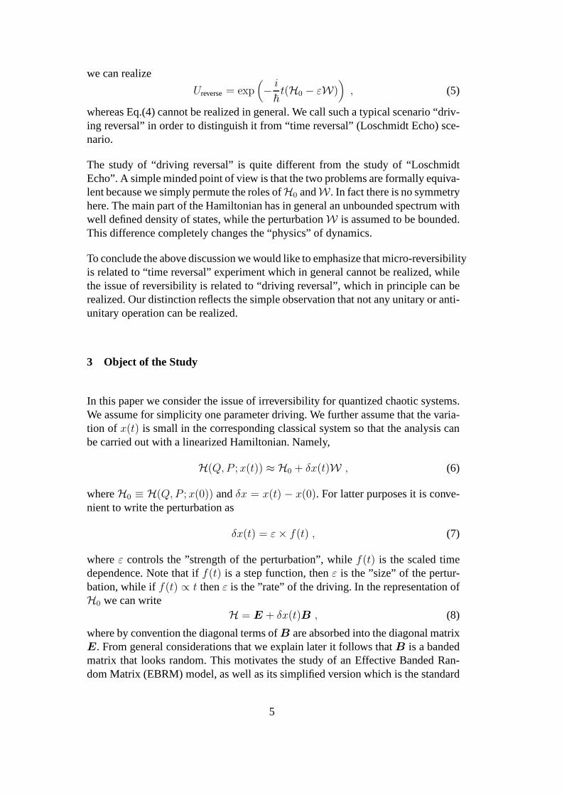
Fig. 2. Equipotential contours (left) of the model HamiltonianH0 for different energies andthe Poincare section (right) of a selected trajectory atE = 3. Some tiny quasi-integrableislands are avoided (mainly at(0, 0)).

4 Modeling

We are interested in quantized chaotic systems that have fewdegrees of freedom.The dynamical system used in our studies is the Pullen-Edmonds model [25,26]. Itconsists of two harmonic oscillators that are nonlinearly coupled. The correspond-ing Hamiltonian is

H(Q, P ; x) =1

2

(

P 21 + P 2

2 + Q21 + Q2

2

)

+ xQ21Q

22 . (14)

The mass and the frequency of the harmonic oscillators are set to one. Without lossof generality we setx(0) = x0 = 1. Later we shall consider classically small defor-mations (δx ≪ 1) of the potential. One can regard this model (14) as a descriptionof a particle moving in a two dimensional well (2DW). The energy E is the only di-mensionless parameter of the classical motion. For high energiesE > 5 the motionof the Pullen-Edmonds model is ergodic. Specifically it was found that the measureof the chaotic component on the Poincare section deviates from unity by no morethan10−3[25,26].

In Figure 2 we display the equipotential contours of the model Hamiltonian (14)with x0 = 1. We observe that the equipotential surfaces are circles butas the en-ergy is increased they become more and more deformed leadingto chaotic motion.Our analysis is focused on an energy window aroundE ∼ 3 where the motion ismainly chaotic. This is illustrated in the right panel of Figure 2 where we report thePoincare section (of the phase space) of a selected trajectory, obtained fromH0 atE = 3. The ergodicity of the motion is illustrated by the Poincar´e section, fillingthe plane except from some tiny quasi- integrable islands.

The perturbation is described byW = Q21Q

22. In the classical analysis there is only

one significant regime for the strength of the perturbation.Namely, the perturbation

9

is considered to be classically small if

δx ≪ εcl , (15)

whereεcl = 1. This is the regime where (classical) linear analysis applies. Namely,within this regime the deformation of the energy surfaceH0 = E can be describedas a linear process (see Eq. (29)).

4.1 Energy levels

Let us now quantize the system. For obvious reasons we are considering a de-symmetrized 1/8 well with Dirichlet boundary conditions onthe linesQ1 = 0,Q2 = 0 andQ1 = Q2. The matrix representation ofH0 in the basis of the un-coupled system is very simple. The eigenstates of the HamiltonianH0 are thenobtained numerically.

As mentioned above, we consider the experiments to take place in an energy win-dow 2.8 < E < 3.1 which is classically small and where the motion is predomi-nantly chaotic. Nevertheless, quantum mechanically, thisenergy window is large,i.e., many levels are found therein. The local mean level spacing ∆(E) at this en-ergy range is given approximately by∆ ∼ 4.3 ~

2. The smallest~ that we canhandle is~ = 0.012 resulting in a matrix size of about4000 × 4000. Unless statedotherwise, all the numerical data presented below correspond to a quantization with~ = 0.012.

As it was previously mentioned in the introduction, the mainfocus of quantumchaos studies has so far been on issues of spectral statistics [14,15]. In this contextit turns out that the sub -~ statistical features of the energy spectrum are ”universal”,and obey the predictions of RMT. In particular we expect thatthe level spacingdistributionP (s) of the ”unfolded” (with respect to∆) level spacingssn = (En+1−En)/∆ will follow with high accuracy the so-calledWigner surmise. For systemswith time reversal symmetry it takes the form [14,27]

Pspacings(s) =π

2s e−

π

4s2

, (16)

indicating that there is a linear repulsion between nearby levels. Non-universal (i.e.system specific) features are reflected only in the large scale properties of the spec-trum and constitute the fingerprints of the underlying classical chaotic dynamics.

The de-symmetrized 2DW model shows time reversal symmetry,and therefore weexpect the distribution to follow Eq.(16). The analysis is carried out only for thelevels contained in the chosen energy window aroundE = 3. Instead of plottingP (s) we show the integrated distributionI(s) =

∫ s0 P (s′)ds′, which is independent

of the bin size of the histogram. In Figure 3 we present our numerical data forI(s)

10

0 1 2 3S

0

0.2

0.4

0.6

0.8

1

I(S

)

0 1 2 3S

-0.04

-0.02

0

0.02

0.04

I th(S

)-I(

S)

Fig. 3. The integrated level spacing distributionI(S) of the unperturbed HamiltonianH0

(~ = 0.012). The dashed line is the theoretical prediction for the GOE.Inset: Differencebetween the theoretical predictionIth(S) and the actual distributionI(S).

while the inset shows the deviations from the theoretical prediction (16). The agree-ment with the theory is fairly good and the level repulsion isclearly observed. Theobserved deviations have to be related on the one hand to the tiny quasi-integrableislands that exist atE = 3 as well as to rather limited level statistics.

4.2 The band-profile

In this subsection we explain that the band-structure ofB is related to the fluctua-tions of the classical motion. This is the major step towardsRMT modeling.

Consider a given ergodic trajectory(Q(t), P (t)) on the energy surfaceH(Q(0), P (0); x0) = E. An example is shown in Fig. 2b. We can associate with ita stochastic-like variable

F(t) = −∂H∂x

(Q(t), P (t), x(t)) , (17)

which for our linearized Hamiltonian is simply the perturbation termF = −W = −Q2

1Q22. It can be interpreted as the generalized force that acts on

the boundary of the 2D well. It may have a non-zero average (“conservative” part)but below we are interested only in its fluctuations.

In order to characterize the fluctuations ofF(t) we introduce the autocorrelationfunctionC(τ)

C(τ) = 〈F(t)F(t + τ)〉 − 〈F2〉 . (18)

The angular brackets denote an averaging which is either micro-canonical oversome initial conditions(Q(0), P (0)) or temporal (due to the assumed ergodicity).The power spectrum for the 2D well model is shown in Fig.4 (seesolid line).

11

-10 -5 0 5 10ω0

0.2

0.4

0.6

0.8

C(ω

)∼

ωcl

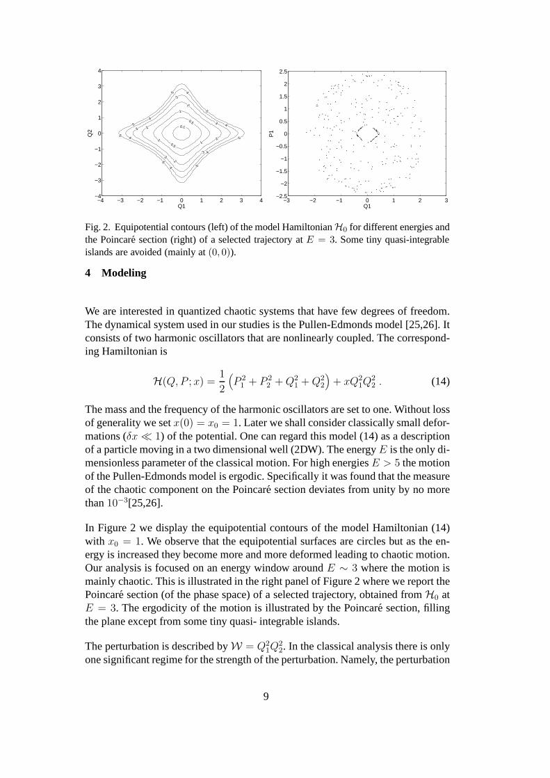
Fig. 4. The classical power-spectrum of the model (14). The classical cut-off frequencyωcl ≃ 7 is indicated by perpendicular dashed lines.

For generic chaotic systems (described by smooth Hamiltonians), the fluctuationsare characterized by a short correlation timeτcl, after which the correlations are neg-ligible. In generic circumstancesτcl is essentially the ergodic time. For our modelsystemτcl ∼ 1.

The power spectrum of the fluctuationsC(ω) is defined by a Fourier transform:

C(ω) =∫ ∞

−∞C(τ) exp(iωτ)dτ . (19)

This power spectrum is characterized by a cut-off frequencyωcl which is inverseproportional to the classical correlation time

ωcl =2π

τcl. (20)

Indeed in the case of our model system we getωcl ∼ 7 which is in agreement withFig.4.

The implication of having a short but non-vanishing classical correlation timeτcl ishaving large but finite bandwidth in the perturbation matrixB. This follows fromthe identity

C(ω) =∑

n

|Bnm|22πδ(

ω − En − Em

~

)

, (21)

which implies

〈|Bnm|2〉 =∆

2π~C(

ω =En − Em

~

)

. (22)

Hence the matrix elements of the perturbation matrixB are extremely small outsideof a band of widthb = ~ωcl/∆.

In the inset of Figure 5 we show a snapshot of the perturbationmatrix |Bnm|2. Itclearly shows a band-structure. At the same figure we also display the band-profiles

12

−8 −6 −4 −2 0 2 4 6 80

0.1

0.2

0.3

0.4

0.5

classicalh=0.030h=0.015

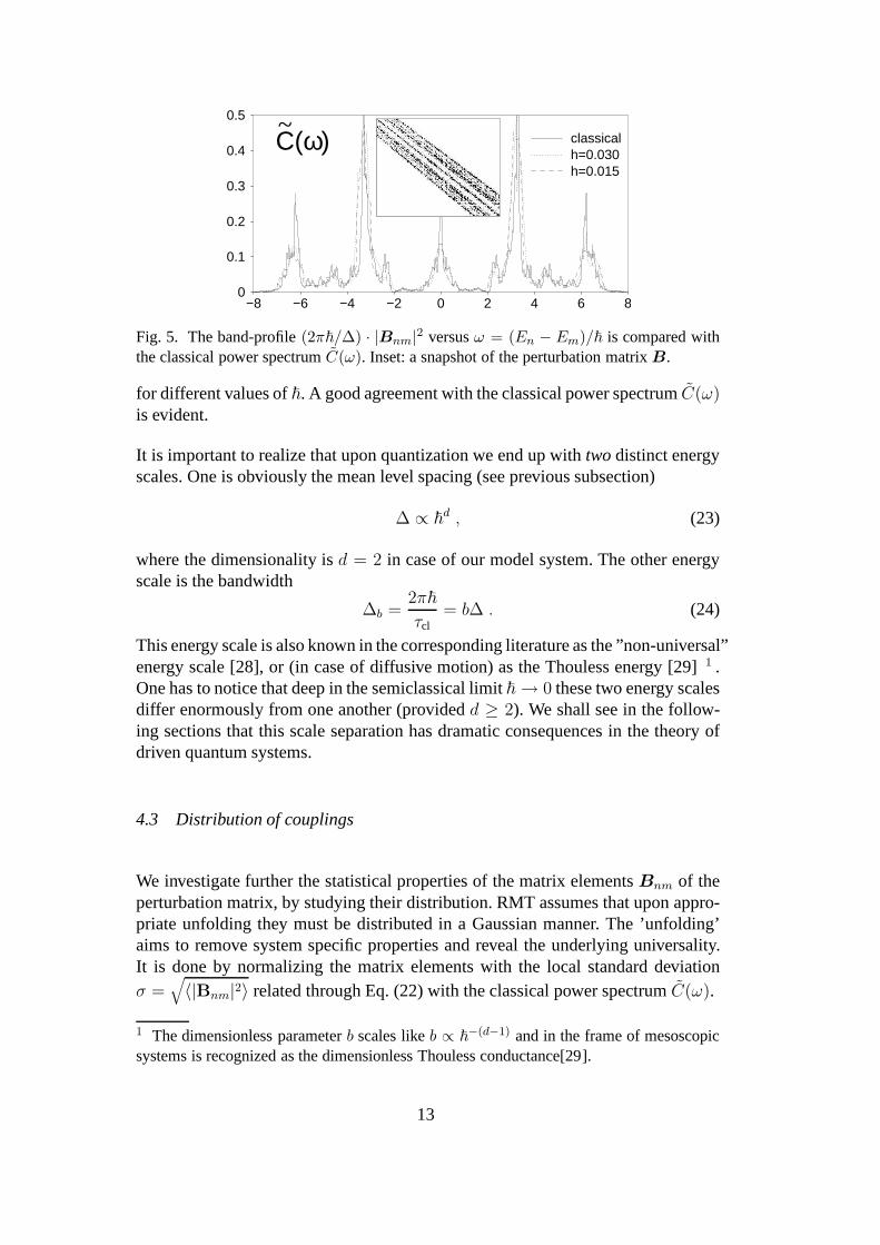
C(ω)~

Fig. 5. The band-profile(2π~/∆) · |Bnm|2 versusω = (En − Em)/~ is compared withthe classical power spectrumC(ω). Inset: a snapshot of the perturbation matrixB.

for different values of~. A good agreement with the classical power spectrumC(ω)is evident.

It is important to realize that upon quantization we end up with twodistinct energyscales. One is obviously the mean level spacing (see previous subsection)

∆ ∝ ~d , (23)

where the dimensionality isd = 2 in case of our model system. The other energyscale is the bandwidth

∆b =2π~

τcl= b∆ . (24)

This energy scale is also known in the corresponding literature as the ”non-universal”energy scale [28], or (in case of diffusive motion) as the Thouless energy [29]1 .One has to notice that deep in the semiclassical limit~ → 0 these two energy scalesdiffer enormously from one another (providedd ≥ 2). We shall see in the follow-ing sections that this scale separation has dramatic consequences in the theory ofdriven quantum systems.

4.3 Distribution of couplings

We investigate further the statistical properties of the matrix elementsBnm of theperturbation matrix, by studying their distribution. RMT assumes that upon appro-priate unfolding they must be distributed in a Gaussian manner. The ’unfolding’aims to remove system specific properties and reveal the underlying universality.It is done by normalizing the matrix elements with the local standard deviationσ =

√

〈|Bnm|2〉 related through Eq. (22) with the classical power spectrumC(ω).

1 The dimensionless parameterb scales likeb ∝ ~−(d−1) and in the frame of mesoscopic

systems is recognized as the dimensionless Thouless conductance[29].

13

-2 0 2q

0

0.1

0.2

0.3

0.4

0.5

P(q

)

Fig. 6. Distribution of matrix elementsq aroundE = 3 rescaled with the averagedband-profile . The solid black line corresponds to a Gaussiandistribution with unit vari-ance while the dashed-dotted line corresponds to a fit from Eq. (25) with a fitting parameterN = 7.8. The quantization corresponds to~ = 0.03.

The existing literature is not conclusive about the distribution of the normalizedmatrix elementsq = Bnm/σ. Specifically, Berry [30] and more recently Prosen[31,32], claimed thatP(q) should be Gaussian. On the other hand, Austin andWilkinson [33] have found that the Gaussian is approached only in the limit ofhigh quantum numbers while for small numbers, i.e., low energies, a different dis-tribution applies, namely

Pcouplings(q) =Γ(N

2)√

πNΓ(N−12

)

(

1 − q2

N

)(N−3)/2

. (25)

This is the distribution of the elements of anN-dimensional vector, distributedrandomly over the surface of anN-dimensional sphere of radius

√N . ForN → ∞

this distribution approaches a Gaussian.

The distributionP(q) for our model is reported in Figure 6. The solid line corre-sponds to a Gaussian of unit variance while the dashed-dotted line is obtained byfitting Eq. (25) to the numerical data usingN as a fitting parameter. We observe thatthe Gaussian resembles better our numerical data although deviations, especiallyfor matrix elements close to zero, can be clearly seen. We attribute these deviationsto the existence of the tiny stability islands in the phase space. Trajectories startedin those islands cannot reach the chaotic sea and vice versa.Quantum mechanicallythe consequence of this would be vanishing matrix elementsBnm which representthe classically forbidden transitions.

14

4.4 RMT modeling

It was the idea of Wigner [12,13] more than forty years ago, tostudy a simplifiedmodel, where the Hamiltonian is given by Eq. (8), and whereB is a BandedRan-domMatrix (BRM) [34,35,36]. The diagonal matrixE has elements which are theordered energiesEn, with mean level spacing∆. The perturbation matrixB hasa rectangularband-profile of band-sizeb. Within the band0 < |n − m| ≤ b theelements are independent random variables given by a Gaussian distribution withzero mean and a varianceσ2 = 〈|Bnm|2〉. Outside the band they vanish. We referto this model as theWigner BRMmodel (WBRM).

Given the band-profile, we can use Eq.(22) in reverse direction to calculate thecorrelation functionC(τ). For the WBRM model we get

C(τ) = 2σ2b sinc (τ/τcl) , (26)

whereτcl = ~/∆b. Thus, there are three parameters(∆, b, σ) that define the WBRMmodel.

The WBRM model can be regarded as asimplifiedlocal description of a true Hamil-tonian matrix. This approach is attractive both analytically and numerically. Ana-lytical calculations are greatly simplified by the assumption that the off-diagonalterms can be treated as independent random numbers. Also from a numerical pointof view it is quite a tough task to calculate the true matrix elements of theB matrix.It requires a preliminary step where the chaoticH0 is diagonalized. Due to memorylimitations one ends up with quite small matrices. For the Pullen-Edmonds modelwe were able to handle matrices of final sizeN = 4000 maximum. This shouldbe contrasted with the WBRM simulations, where using self -expanding algorithm[37,17] we were able to handle system sizes up toN = 100000 along with signifi-cantly reduced CPU time.

We would like to stress again that the underlying assumptionof WBRM, namelythat the off-diagonal elements areuncorrelatedrandom numbers, has to be treatedwith extreme care.

The WBRM model involves an additional simplification. Namely, one assumes thatB has arectangularband-profile. A simple inspection of the band-profile of ourmodel Eq. (14) shows that this is not the case (see Fig. 5). We eliminate this simpli-fication by introducing a RMT model that is even closer to the dynamical one. Tothis end, we randomize the signs of the off-diagonal elements of the perturbationmatrixB keeping its band-structure intact. This procedure leads toa random modelthat exhibits only universal properties while it lack any semiclassical limit. We willrefer to it as theeffectivebanded random matrix model (EBRM).

15

5 The Parametric Evolution of the Eigenfunctions

As we change the parameterδx in the Hamiltonian Eq. (8), the instantaneous eigen-states|n(x)〉 evolve and undergo structural changes. In order to understand theactual dynamics, it is important to understand these structural changes. This leadsto the introduction of

P (n|m) = |〈n(x)|m(x0)〉|2 , (27)

which is easier to analyze thanPt(n|n0). Up to some trivial scaling and shiftingP (n|m) is essentially the local density of states (LDoS):

P (E|m) =∑

n

|〈n(x)|m(x0)〉|2δ(E − En) . (28)

The averaged distributionP (r) is defined in complete analogy with the definition ofPt(r). Namely, we use the notationr = n − m, and average over severalm stateswith roughly the same energyEm ∼ E.

GenericallyP (r) undergoes the following structural changes as a function ofgrow-ing δx. We first summarize the generic picture, which involves the parametric scalesεc andεprt. and the approximationsPFOPT, Pprt, andPsc. Then we discuss how to de-termine these scales, and what these approximations are.

• The first order perturbative theory (FOPT) regime is defined as the rangeδx < εc

where we can use FOPT to get an approximation that we denote asP () ≈ PFOPT.• The (extended) perturbative regime is defined as the rangeεc < δx < εprt where

we can use perturbation theory (to an infinite order) to get a meaningful approx-imation that we denote asP () ≈ Pprt. ObviouslyPprt reduces toPFOPT in theFOPT regime.

• The non-perturbative regime is defined as the rangeδx > εprt where perturbationtheory becomes non-applicable. In this regime we have to useeither RMT orsemiclassics in order to get an approximation that we denoteasP () ≈ Psc.

Irrespective of these structural changes, it can be proved that the variance ofP (r)is strictly linear and given by the expression

δE(δx) =√

C(0) δx ≡ δEcl . (29)

The only assumption that underlines this statement isδx ≪ εcl. It reflects the lineardeparture of the energy surfaces.

16

5.1 Approximations forP (n|m)

The simplest regime is obviously the FOPT regime where, forP (n|m), we can usethe standard textbook approximationPFOPT(n|m) ≈ 1 for n = m, while

PFOPT(n|m) =δx2 |Bnm|2(En−Em)2

, (30)

for n 6= m. If outside of the band we haveBnm = 0, as in the WBRM model, thenPFOPT(r) = 0 for |r| > b. To find the higher order tails (outside of the band) wehave to go to higher orders in perturbation theory. Obviously this approximationmakes sense only as long asδx < εc where

εc = ∆/σ ∼ ~(1+d)/2 , (31)

andd is the degrees of freedom of our system (d = 2 for the 2D well model).

If δx > εc but not too large then we still have tail regions which are described byFOPT. This is a non-trivial observation which can be justified by using perturbationtheory to infinite order. Then we can argue that a reasonable approximation is

Pprt(n|m) =δx2 |Bnm|2

(En−Em)2 + Γ2, (32)

whereΓ is evaluated by imposing normalization ofPprt(n|m). In the case of WBRMmodelΓ = (σδx/∆)2 ×∆. The appearance ofΓ in the above expression cannot beobtained from anyfinite-orderperturbation theory: Formally it requires summationto infinite order. Outside of the bandwidth the tails decay faster than exponentially.Note thatPprt(n|m) is a Lorentzian in the case of a flat bandwidth (WBRM model),while in the general case it can be described as a ”core-tail”structure.

Obviously the above approximation makes sense only as long asΓ(δx) < ∆b. Thisexpression assumes that the bandwidth∆b is sharply defined, as in the WBRMmodel. By elimination this leads to the determination ofεprt, which in case of theWBRM model is simply

εprt =√

b εc ∼~

τcl

√

C(0). (33)

In more general cases the bandwidth is not sharply defined. Then we have to definethe perturbative regime using a practical numerical procedure. The natural defini-tion that we adopt is as follows. We calculate the spreadingδE(δx), which is alinear function. Then we calculateδEprt(δx), using Eq.(32)). This quantity alwayssaturates for largeδx because of having finite bandwidth. We compare it to theexactδE(δx), and defineεprt for instance as the80% departure point.

17

-300 -200 -100 0 100 200 300-20

-15

-10

-5

0

-300 -200 -100 0 100 200 300-10

-5

ln[P

(r)]

-300 -200 -100 0 100 200 300-10

-5

-2000 -1000 0 1000 2000r

-10

-5

a)

b)

c)

d)

∆b

∆b

∆b

Γ

∆b

Fig. 7. The parametric evolution of eigenstates of a WBRM model with σ = 1 andb = 50:(a) Standard perturbative regime corresponding toǫ = 0.01, (b) Extended perturbativeregime withǫ = 2 (c) Non-perturbative (ergodic) regime withǫ = 12 and (d) localizedregime withǫ = 1. In (a-c) the mean level spacing∆ = 1 while in (d) ∆ = 10−3. Thebandwidth∆b = ∆ × b is indicated in all cases. In (b) the blue dashed line corresponds toa Lorentzian withΓ ≈ 16 ≪ ∆b while in (a) we haveΓ ≈ 10−4 ≪ ∆ which thereforereduces to the standard FOPT result.

18

-20

-10

0

-20

-10

0

ln[P

(r)]

-600 -400 -200 0 200 400 600r

-20

-10

0

P(r)P

RMT(r)

Pprt

(r)

Pcl(r)

a)

b)

c)

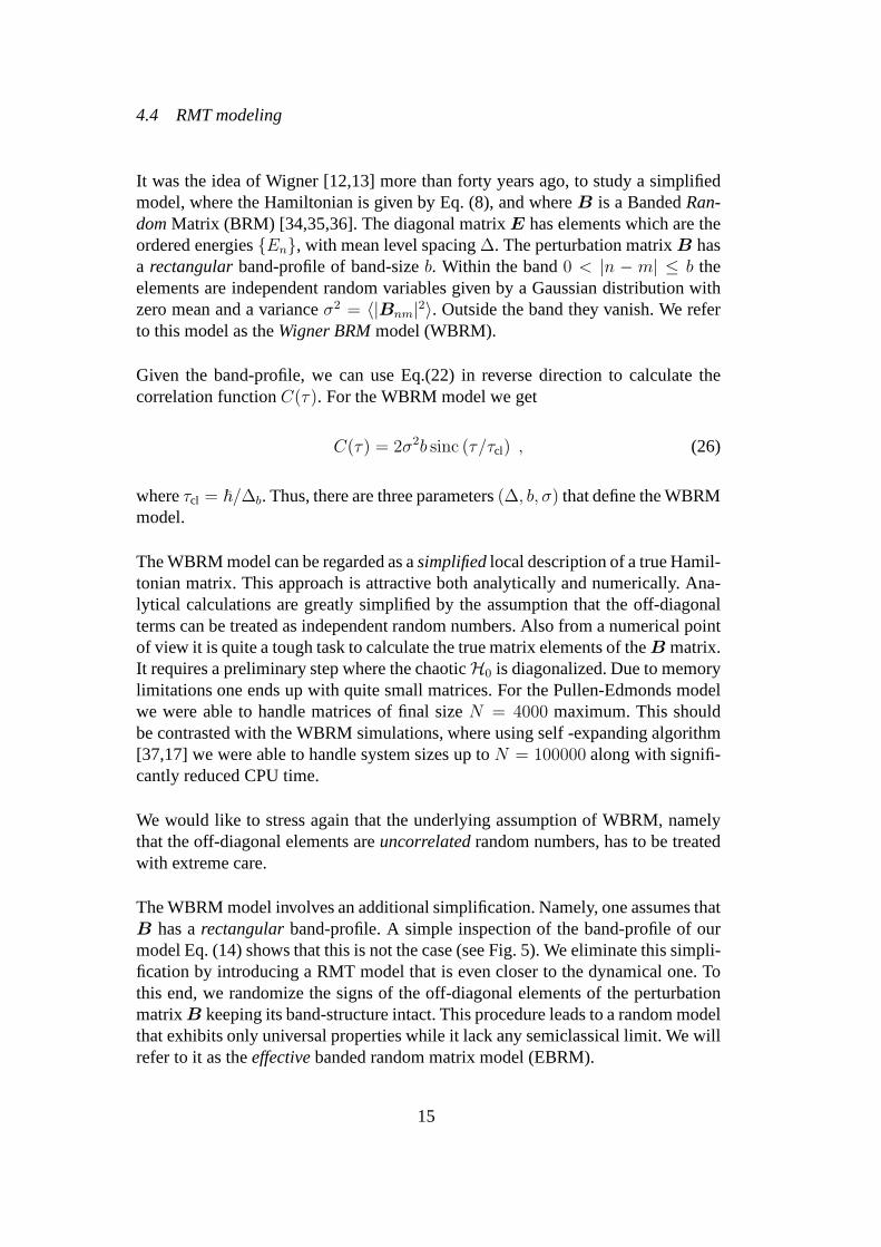
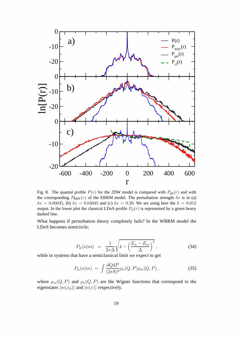
Fig. 8. The quantal profileP (r) for the 2DW model is compared withPprt(r) and withthe correspondingPRMT(r) of the EBRM model. The perturbation strengthδx is in (a)δx = 0.00035, (b) δx = 0.04945 and (c)δx = 0.29. We are using here the~ = 0.012output. In the lower plot the classical LDoS profilePcl(r) is represented by a green heavydashed line.

What happens if perturbation theory completely fails? In the WBRM model theLDoS becomes semicircle:

Psc(n|m) =1

2π∆

√

4 −(

En − Em

∆

)2

, (34)

while in systems that have a semiclassical limit we expect toget

Psc(n|m) =∫

dQdP

(2π~)dρn(Q, P )ρm(Q, P ) , (35)

whereρm(Q, P ) and ρn(Q, P ) are the Wigner functions that correspond to theeigenstates|m(x0)〉 and|n(x)〉 respectively.

19

5.2 TheP (n|m) in practice

There are some findings that go beyond the above generic picture and, for com-pleteness, we mention them. The first one is the ”localization regime” which isfound in the case of the WBRM model forε > εloc. where

εloc = b3/2εc . (36)

In this regime it is important to distinguish between the non-averagedP (n|m) andthe averagedP (r) because the eigenfunctions are non-ergodic but rather localized.This localization is not reflected in the LDoS which is still asemicircle. A typi-cal eigenstate is exponentially localized within an energyrangeδEξ = ξ∆ muchsmaller thanδEcl. The localization length isξ ≈ b2. In actual physical applicationsit is not clear whether there is such a type of localization. The above scenario forthe WBRM model is summarized in Fig. 7 where we plotP (n|m) in the variousregimes. The localized regime is not an issue in the present work and therefore wewill no further be concerned with it.

The other deviation from the generic scenario, is the appearance of a non-universal”twilight regime” which can be found for some quantized systems [38]. In thisregime a co-existence of a perturbative and a semiclassicalstructure can be ob-served. For the Pullen-Edmonds model (14) there is no such distinct regime.

For the Hamiltonian model described by Eq. (14) the borders between the regimescan be estimated [19]. Namelyεc ≈ 3.8~

3/2 andεprt ≈ 5.3~. In Fig. 8 we reportthe parametric evolution of the eigenstates for the Hamiltonian model of Eqs. (14)and we compare the outcomes with the results of the EBRM model[19]. Despitethe overall quantitative agreement, some differences can be detected:

• In the FOPT regime (see Fig. 8a), the RMT strategy fails in thefar tails regime∆× |r| > ∆b where system specific interference phenomena become important.

• In the extended perturbative regime (see Fig. 8b) the line-shape of the averagedwavefunctionP (n|m) is different from Lorentzian. Still the general features ofPprt (core-tail structure) can be detected. In a sense, Wigner’sLorentzian (32) is aspecial case of core-tail structure. Finally, as in the standard perturbative regimeone observes that the far-tails are dominated by either destructive interference(left tail), or by constructive interference (right tail).

• Deep in the non-perturbative regime (ε > εprt ) the overlapsP (n|m) are wellapproximated by the semiclassical expression. The exact shape is determined bysimple classical considerations [19,39]. This is in contrast to the WBRM modelwhich does not have a classical limit.

20

6 Linear Response Theory

The definition of regimes for driven systems is more complicated than the corre-sponding definition in case of LDoS theory. It is clear that for short times we al-ways can use time-dependent FOPT. The question is, of course, what happens next.There we have to distinguish between two types of scenarios.One type of scenariois wavepacket dynamicsfor which the dynamics is a transient from a preparationstate to some new ergodic state. The second type of scenario is persistent driving,either linear driving (x = ε) or periodic driving (x(t) = ε sin(Ωt)). In the lattercase the strength of the perturbation depends on the rate of the driving, not juston the amplitude. The relevant question iswhether the long time dynamics canbe deduced from the short time analysis. To say that the dynamics is of perturba-tive nature means that the short time dynamics can be deducedfrom FOPT, whilethe long time dynamics can be deduced on the basis of a Markovian (stochastic)assumption. The best known example is the derivation of the exponential Wignerlaw for the decay of metastable state. The Fermi-Golden-Rule (FGR) is used todetermine the initial rate for the escaping process, and then the long-time result isextrapolated by assuming that the decay proceeds in a stochastic-like manner. Simi-lar reasoning is used in deriving the Pauli master equation which is used to describethe stochastic-like transitions between the energy levelsin atomic systems.

A related question to the issue of regimes is the validity of Linear Response Theory(LRT). In order to avoid ambiguities we adopt here a practical definition. When-ever the result of the calculation depends only on the two point correlation func-tion C(τ), or equivalently only on the band-profile of the perturbation (which isdescribed byC(ω)), then we refer to it as ”LRT”. This implies that higher ordercorrelations are not expressed. There is a (wrong) tendencyto associate LRT withFOPT. In fact the validity of LRT is not simply related to FOPT. We shall clarifythis issue in the next section.

For bothδE(t) andP(t) we have ”LRT formulas” which we discuss in the nextsections. Writing the driving pulse asδx(t) = εf(t) for the spreading we get:

δE2(t) = ε2 ×∫ ∞

−∞

dω

2πC(ω)Ft(ω) , (37)

while for the survival probability we have

P(t) = exp

(

−ε2 ×∫ ∞

−∞

dω

2πC(ω)

Ft(ω)

(~ω)2

)

. (38)

Two spectral functions are involved: One is the power spectrum C(ω) of the fluctu-ations defined in Eq. (19), and the otherFt(ω) is the spectral content of the driving

21

pulse which is defined as

Ft(ω) =∣

∣

∣

∣

∫ t

0dt′f(t′)e−iωt′

∣

∣

∣

∣

2

. (39)

Here we summarize the main observations regarding the nature of wavepacket dy-namics in the various regimes:

• FOPT regime: In this regimeP(t) ∼ 1 for all time, indicating that all probabilityis all the time concentrated on the initial level. An alternative way to identify thisregime is fromδEcore(t) which is trivially equal to∆.

• Extended perturbative regime: The appearance of a core-tail structure which ischaracterized by separation of scales∆ ≪ δEcore(t) ≪ δE(t) ≪ ∆b. The coreis of non-perturbative nature, but the varianceδE2(t) is still dominated by thetails. The latter are described by perturbation theory.

• Non-perturbative regime: The existence of this regime is associated with havingthe finite energy scale∆b. It is characterized by∆b ≪ δEcore(t) ∼ δE(t). Asimplied by the terminology, perturbation theory (to any order) is not a valid toolfor the analysis of the energy spreading. Note that in this regime, the spreadingprofile is characterized by a single energy scale (δE ∼ δEcore).

6.1 The energy spreadingδE(t)

Of special importance for understanding quantum dissipation is the theory for thevarianceδE2(t) of the energy spreading. HavingδE(t) ∝ ǫ meanslinear response.If δE(t)/ǫ depends onǫ, we call it “non-linear response”. In this paragraph weexplain that linear response theory (LRT) is based on the “LRT formula” Eq.(37)for the spreading. This formula has a simple classical derivation (see Subsection6.2 below).

From now on it goes without saying that we assume theclassicalconditions for thevalidity of Eq.(37) are satisfied (no~ involved in such conditions). The questionis what happens to the validity of LRT once we “quantize” the system. In previouspublications[8,10,11,19], we were able to argue the following:

(A) The LRT formula can be trusted in the perturbative regime, with the exclusionof the adiabatic regime.

(B) In the sudden limit the LRT formula can also be trusted in the non-perturbativeregime.

(C) In general the LRT formula cannot be trusted in the non-perturbative regime.(D) The LRT formula can be trusted deep in the non-perturbative regime, provided

the system has a classical limit.

For a system that does not have a classical limit (Wigner model) we were able todemonstrate [8,10,11] that LRT fails in the non-perturbative regime. Namely, for

22

the WBRM model the responseδE(t)/ǫ becomesǫ dependent for largeǫ, meaningthat the response is non-linear. Hence the statement in item(C) above has beenestablished. We had argued that the observed non-linear response is the result of aquantal non-perturbative effect. Do we have a similar type of non-linear responsein the case ofquantized chaoticsystems? The statement in item (D) above seems tosuggest that the observation of such non-linearity is not likely. Still, it was argued in[11] that this does not exclude the possibility of observinga “weak” non-linearity.

The immediate (naive) tendency is to regard LRT as the outcome of quantum me-chanical first order perturbation theory (FOPT). In fact theregimes of validity ofFOPT and of LRT do not coincide. On the one hand we have the adiabatic regimewhere FOPT is valid as a leading order description, but not for response calculation.On the other hand, the validity of Eq.(37) goes well beyond FOPT. This leads tothe (correct) identification [7,8,11] of what we call the “perturbative regime”. Theborder of this regime is determined by the energy scale∆b, while∆ is not involved.Outside of the perturbative regime we cannot trust the LRT formula. However, aswe further explain below, the fact that Eq.(37) is not valid in the non-perturbativeregime, does not imply that itfails there.

We stress again that one should distinguish between “non-perturbative response”and “non-linear response”. These are not synonyms. As we explain in the nextparagraph, the adiabatic regime is “perturbative” but “non-linear”, while the semi-classical limit is “non-perturbative” but “linear”.

In the adiabatic regime, FOPT implies zero probability to make a transitions toother levels. Therefore, to the extent that we can trust the adiabatic approxima-tion, all probability remains concentrated on the initial level. Thus, in the adiabaticregime, Eq.(37) is not a valid formula: It is essential to usehigher orders of per-turbation theory, and possibly non-perturbative corrections (Landau-Zener [1,2]),in order to calculate the response. Still, FOPT provides a meaningful leading orderdescription of the dynamics (i.e. having no transitions), and therefore we do notregard the adiabatic non-linear regime as “non-perturbative”.

In thenon-perturbative regimethe evolution ofPt(n|m) cannot be extracted fromperturbation theory: not in leading order, neither in any order. Still it does not neces-sarily imply a non-linear response. On the contrary: The semiclassical limit is con-tained in the deep non-perturbative regime [8,11]. There, the LRT formula Eq.(37)is in fact valid. But its validity isnot a consequence of perturbation theory, butrather the consequence ofquantal-classical correspondence(QCC).

In the next subsection we will present a classical derivation of the general LRTexpression (37). In Subsection 6.3 we derive it using first order perturbation theory(FOPT). In Subsection 6.5 we derive the corresponding FOPT expression for thesurvival probability.

23

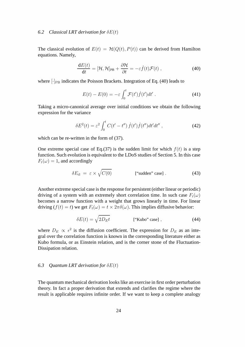
6.2 Classical LRT derivation forδE(t)

The classical evolution ofE(t) = H(Q(t), P (t)) can be derived from Hamiltonequations. Namely,

dE(t)

dt= [H,H]PB +

∂H∂t

= −εf(t)F(t) , (40)

where[·]PB indicates the Poisson Brackets. Integration of Eq. (40) leads to

E(t) − E(0) = −ε∫ t

0F(t′)f(t′)dt′ . (41)

Taking a micro-canonical average over initial conditions we obtain the followingexpression for the variance

δE2(t) = ε2∫ t

0C(t′ − t′′) f(t′)f(t′′)dt′dt′′ , (42)

which can be re-written in the form of (37).

One extreme special case of Eq.(37) is the sudden limit for which f(t) is a stepfunction. Such evolution is equivalent to the LDoS studies of Section 5. In this caseFt(ω) = 1, and accordingly

δEcl = ε ×√

C(0) [“sudden” case]. (43)

Another extreme special case is the response for persistent(either linear or periodic)driving of a system with an extremely short correlation time. In such caseFt(ω)becomes a narrow function with a weight that grows linearly in time. For lineardriving (f(t) = t) we getFt(ω) = t × 2πδ(ω). This implies diffusive behavior:

δE(t) =√

2DEt [“Kubo” case] , (44)

whereDE ∝ ǫ2 is the diffusion coefficient. The expression forDE as an inte-gral over the correlation function is known in the corresponding literature either asKubo formula, or as Einstein relation, and is the corner stone of the Fluctuation-Dissipation relation.

6.3 Quantum LRT derivation forδE(t)

The quantum mechanical derivation looks like an exercise infirst order perturbationtheory. In fact a proper derivation that extends and clarifies the regime where theresult is applicable requires infinite order. If we want to keep a complete analogy

24

with the classical derivation we should work in the adiabatic basis [7]. (For a briefderivation see Appendix D of [9]).

In the following presentation we work in a ”fixed basis” and assumef(t) = f(0) =0. We use the standard textbook FOPT expression for the transition probabilityfrom an initial statem to any other staten. This is followed by integration by parts.Namely,

Pt(n|m) =ε2

~2|Bnm|2

∣

∣

∣

∣

∣

∣

t∫

0

dt′f(t′)ei(En−Em)t′/~

∣

∣

∣

∣

∣

∣

2

=ε2

~2|Bnm|2

Ft(ωnm)

(ωnm)2, (45)

whereωnm = (En − Em)/~. Now we calculate the variance and use Eq. (22) so asto get

δE2(t) =∑

n

Pt(n|m)(En − Em)2

= ε2∫ ∞

−∞

dω

2πC(ω) Ft(ω) . (46)

6.4 Restricted QCC

The FOPT result forδE(t) is exactlythe same as the classical expression Eq. (37).It is important to realize that there is no~-dependence in the above formula. Thiscorrespondence does not hold for the higherk−moments of the energy distribution.If we use the above FOPT procedure we get that the latter scaleas~

k−2.

We call the quantum-classical correspondence for the second moment ”restrictedQCC”. It is a very robust correspondence [11]. This should becontrasted with ”de-tailed QCC” that applies only in the semiclassical regime wherePt(n|m) can beapproximated by a classical result (and not by a perturbative result).

6.5 Quantum LRT derivation forP(t)

With the validity of FOPT assumed we can also calculate the time-decay of thesurvival probabilityP(t). From Eq. (45) we get:

p(t) ≡∑

n(6=n0)

Pt(n|m) = ε2∫ ∞

−∞

dω

2πC(ω)

Ft(ω)

(~ω)2. (47)

25

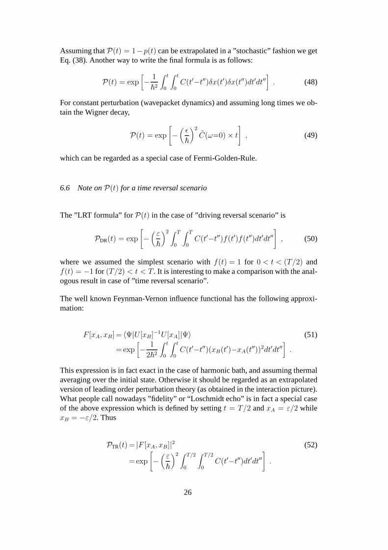
Assuming thatP(t) = 1−p(t) can be extrapolated in a ”stochastic” fashion we getEq. (38). Another way to write the final formula is as follows:

P(t) = exp[

− 1

~2

∫ t

0

∫ t

0C(t′−t′′)δx(t′)δx(t′′)dt′dt′′

]

. (48)

For constant perturbation (wavepacket dynamics) and assuming long times we ob-tain the Wigner decay,

P(t) = exp

[

−(

ǫ

~

)2

C(ω=0) × t

]

, (49)

which can be regarded as a special case of Fermi-Golden-Rule.

6.6 Note onP(t) for a time reversal scenario

The ”LRT formula” forP(t) in the case of ”driving reversal scenario” is

PDR(t) = exp

[

−(

ε

~

)2 ∫ T

0

∫ T

0C(t′−t′′)f(t′)f(t′′)dt′dt′′

]

, (50)

where we assumed the simplest scenario withf(t) = 1 for 0 < t < (T/2) andf(t) = −1 for (T/2) < t < T . It is interesting to make a comparison with the anal-ogous result in case of ”time reversal scenario”.

The well known Feynman-Vernon influence functional has the following approxi-mation:

F [xA, xB] = 〈Ψ|U [xB]−1U [xA]|Ψ〉 (51)

= exp[

− 1

2~2

∫ t

0

∫ t

0C(t′−t′′)(xB(t′)−xA(t′′))2dt′dt′′

]

.

This expression is in fact exact in the case of harmonic bath,and assuming thermalaveraging over the initial state. Otherwise it should be regarded as an extrapolatedversion of leading order perturbation theory (as obtained in the interaction picture).What people call nowadays ”fidelity” or “Loschmidt echo” is in fact a special caseof the above expression which is defined by settingt = T/2 andxA = ε/2 whilexB = −ε/2. Thus

PTR(t) = |F [xA, xB]|2 (52)

=exp

[

−(

ε

~

)2 ∫ T/2

0

∫ T/2

0C(t′−t′′)dt′dt′′

]

.

26

Assuming a very short correlation time one obtains

PTR(T ) = exp

[

−1

2

(

ǫ

~

)2

C(ω=0) × T

]

, (53)

which again can be regarded as a special variation of the Fermi-Golden-Rule (butnote the pre-factor1/2).

6.7 The survival probability and the LDoS

For constant perturbation it is useful to remember thatP(t) LDoS as follows:

P(t)≡∣

∣

∣〈n(x0)|e−iH(x)t/~|n(x0)〉∣

∣

∣

2

=

∣

∣

∣

∣

∣

∑

m

e−iEm(x)t/~|〈m(x)|n(x0)〉|2∣

∣

∣

∣

∣

2

=

∣

∣

∣

∣

∫ ∞

∞P (E|m)e−iEt/~dE

∣

∣

∣

∣

2

. (54)

This implies that a Wigner decay is associated with a Lorentzian approximationfor the LDoS. In the non-perturbative regime the LDoS is not aLorentzian, andtherefore one should not expect an exponential. In the semiclassical regime theLDoS shows system specific features and therefore the decay of P(t) becomesnon-universal.

7 Wavepacket Dynamics for Constant Perturbation

The first evolution scheme that we are investigating here is the so-calledwavepacketdynamics. The classical picture is quite clear [17,18]: The initial preparation isassumed to be a micro-canonical distribution that is supported by the energy surfaceH0(Q, P ) = E(0). TakingH to be a generator for the classical dynamics, thephase-space distribution spreads away from the initial surface fort > 0. ‘Points’of the evolving distribution move upon the energy surfaces of H(Q, P ). Thus, theenergyE(t) = H0(Q(t), P (t)) of the evolving distributions spreads with time.Using the LRT formula Eq.(39) for rectangular pulsef(t′) = 1 for 0 < t′ < t weget

Ft(ω) =∣

∣

∣1 − e−iωt∣

∣

∣

2= (ωt)2sinc

(

ωt

2

)

, (55)

and henceδEcl(t) = ε ×

√

2(C(0) − C(t)) . (56)

27

-4 -2 0 2ln(t)

-3

-2

-1

0

ln(δ

E(t

)/ε)

classicalε = 0.00035ε = 0.02945ε = 0.1ε = 0.23ε = 0.3

2DW

-4 -2 0 2ln(t)

-3

-2

-1

0

ln(δE(t)/ε)

EBRM

Fig. 9. Simulations of wavepacket dynamics for the 2DW model(left panel) and for thecorresponding EBRM model (right panel). The energy spreading δE(t) (normalized withrespect to the perturbation strengthǫ) is plotted as a function of time for various perturba-tion strengthsǫ corresponding to different line-types (the same in both panels). The classicalspreadingδEcl(t) (thick dashed line) is plotted in both panels as a reference.

For short timest ≪ τcl we can expand the correlation function asC(t) ≈ C(0) −12C ′′(0)t2, leading to a ballistic evolution. Then, fort ≫ τcl, due to ergodicity, a

‘steady-state distribution’ appears, where the evolving ‘points’ occupy an ‘energyshell’ in phase-space. The thickness of this energy shell equalsδEcl. Thus, we havea crossover from ballistic energy spreading to saturation:

δE(t) ≈

√2(δEcl/τcl) t for t < τcl

√2δEcl for t > τcl

. (57)

Figure 9 shows the classical energy spreading (heavy dashedline) for the 2DWmodel. In agreement with Eq. (57) we see thatδEcl(t) is first ballistic and then sat-urates. The classical dynamics is fully characterized by the two classical parametersτcl andδEcl.

7.1 The quantum dynamics

Let us now look at the quantized 2DW model. The quantum mechanical data arereported in Fig. 9 (left panel) where different curves correspond to various pertur-bation strengthsε. As in the classical case (heavy dashed-line) we observe an initialballistic-like spreading [18] followed by saturation. This could lead to the wrongimpression that the classical and the quantum spreading areof the same nature.However, this is definitely not the case.

In order to detect the different nature of quantum ballistic-like spreading, one hasto inquire measures that are sensitive to the structure of the profile, such as thecore-widthδEcore(t). In Fig. 10 we present our numerical data for the 2DW model.If the spreading were of a classical type, it would imply thatthe spreading pro-

28

-4 -2 0 2ln(t)

-6

-4

-2

0

ln( δ

Eco

re(t

)/ε)

2DW

Fig. 10. Simulations of wavepacket dynamics for the 2DW model. The evolution of the(normalized) core widthδEcore(t) is plotted as a function of time. The classical expectationis represented by a thick dashed line for the sake of comparison. Asǫ becomes larger it isapproached more and more. We use the same set of parameters asin Fig. 9.

file is characterized by a single energy scale. In such a case we would expect thatδEcore(t) ∼ δE(t). Indeed this is the case forε > εprt with the exclusion of veryshort times: The largerε is the shorter the quantal transient becomes. In the per-turbative regimes, in contrast to the semiclassical regime, we have a separation ofenergy scalesδEcore(t) ≪ δE(t). In the perturbative regimesδE(t) is determinedby the tails, and it is not sensitive to the size of the ‘core’ region.

Using the LRT formula forP(t) we get, for short times (t ≪ τcl) during theballistic-like stage

P(t) = exp

(

−C(τ=0) ×(

ǫt

~

)2)

, (58)

while for long times (t ≫ τcl) we have the FGR decay of Eq.(49). Can we trustthese expressions? Obviously FOPT can be trusted as long asP(t) ∼ 1. This canbe converted into an inequalityt < tprt where

tprt =(

εprt

ε

)ν=1,2

τcl . (59)

The powerν = 1 applies to the non-perturbative regime where the breakdownofP(t) happens to be beforeτcl. The powerν = 2 applies to the perturbative regimewhere the breakdown ofP(t) happens afterτcl at tprt = ~/Γ, i.e. after the ballistic-like stage.

The long term behavior ofP(t) in the non-perturbative regime is not the Wignerdecay. It can be obtained by Fourier transform of the LDoS. Inthe non-perturbativeregime the LDoS is characterized by the single energy scaleδEcl ∝ δx. Hence thedecay in this regime is characterized by a semiclassical time scale2π~/δEcl.

29

7.2 The EBRM dynamics

Next we investigate the applicability of the RMT approach todescribe wavepacketdynamics [17,18] and specifically the energy spreadingδE(t). At first glance, wemight be tempted to speculate that RMT should be able, at least as far asδE(t) isconcerned, to describe the actual quantum picture. After all, we have seen in Sub-section 6.1 that the quantum mechanical LRT formula (46) forthe energy spreadinginvolves as its only input the classical power spectrumC(ω). Thus we would ex-pect that an effective RMT model with the same band-profile would lead to thesameδE(t).

However, things are not so trivial. In Figure 9 we show the numerical results forthe EBRM model2 . In the standard and in the extended perturbative regimes weobserve a good agreement with Eq.(46). This is not surprising as the theoreticalprediction was derived via FOPT, where correlations between off-diagonal ele-ments are not important. In this sense the equivalence of the2DW model andthe EBRM model is trivial in these regimes. But as soon as we enter the non-perturbative regime, the spreadingδE(t) shows a qualitatively different behaviorfrom the one predicted by LRT: After an initial ballistic spreading, we observe apremature crossover to a diffusive behavior

δE(t) =√

2DEt . (60)

The origin of the diffusive behavior can be understood in thefollowing way. Upto time tprt the spreadingδE(t) is described accurately by the FOPT result (46).At t ∼ tprt the evolving distribution becomes as wide as the bandwidth,and wehaveδEcore ∼ δE ∼ ∆b rather thanδEcore ≪ δE ≪ ∆b. We recall that in thenon-perturbative regime FOPT is subjected to a breakdown before reaching satura-tion. The following simple heuristic picture turns out to becorrect. Namely, oncethe mechanism for ballistic-like spreading disappears, a stochastic-like behaviortakes its place. The stochastic energy spreading is similarto a random-walk pro-cess where the step size is of the order∆b, with transient timetprt. Therefore wehave a diffusive behaviorδE(t)2 = 2DEt with

DE = C · ∆2b/tprt = C · ∆2b5/2εσ/~ ∝ ~ (61)

whereC is some numerical pre-factor. This diffusion is not of classical nature,since in the~ → 0 limit we get DE → 0. The diffusion can go on until the en-ergy spreading profile ergodically covers the whole energy shell and saturates to aclassical-like steady state distribution. The timeterg for which we get ergodizationis characterized by the condition(DEt)

1/2 < δEcl, leading to

terg = b−3/2~ ε σ/∆2 ∝ 1/~ . (62)

2 The same qualitative results were found also for the prototype WBRM model, see [17].

30

τcl

Ht ergodicWigner

transient ttprterg

recurrenceslocalization

tprt

tsdn

tdiffusion τcl

Ht Wigner

transient tprt

recurrences

tprt

∆/σ ∆/σbb1/2 ε∆/σ ε3/2c prt

terg

ergodicbrk

ballistic spreading

ballistic−like spreading

sdnt

ballistic−like spreading

ε ε

=

Fig. 11. A diagram that illustrates the various time scales in wavepacket dynamics, de-pending on the strength of the perturbationε. The diagram on the left refers to the WBRMmodel, while that on the right is for a quantized system that has a classical limit. The twocases differ in the non-perturbative regime (largeε): In the case of a quantized model wehave a genuine ballistic behavior which reflects detailed QCC, while in the RMT case wehave a diffusive stage. In the latter case the times scaletsdn marks the crossover from re-versible to non-reversible diffusion. This time scale can be detected in a driving reversalscenario as explained in the next section. For further discussion of this diagram see thetext, and in particular the concluding section of this paper.

For completeness we note that forε > εloc there is no ergodization but ratherdynamical (”Anderson” type) localization. Hence, in the latter case,terg is replacedby the break-timetbrk. The various regimes and time scales are illustrated by thediagram presented in Fig. 11.

8 Driving Reversal Scenario

A thorough understanding of the one-period driving reversal scenario [10] is bothimportant within itself, and for constituting a bridge towards a theory dealing withthe response to periodic driving [8]. In the following subsection we present ourresults for the prototype WBRM model, while in Subsection 8.2 we consider the2DW model and compare it to the corresponding EBRM model. TheEBRM isbetter for the purpose of making comparisons with the 2DW, while the WBRMis better for the sake of quantitative analysis (the ”physics” of the EBRM and theWBRM models is, of course, the same).

The quantities that monopolize our interest are the energy spreadingδE(t) and thesurvival probabilityP(t). In Figs. 12 and 13 we present representative plots. From alarge collection of such data that collectively span a very wide range of parameters,we extract results forδE(T ), for P(T ), and for the corresponding compensationtimes. These are presented in Figs. 12,13,14,15,16 and 17.

31

0 0.1 0.2 0.3 0.4t

0

0.1

0.2

0.3δE

(t)

/ ε

ε = 0.1ε = 0.13ε = 0.16ε = 0.23ε = 0.26ε = 0.29

0

0.1

0.2

0.3

ε = 0.00035ε = 0.00105ε = 0.00315ε = 0.00945ε = 0.002945ε = 0.004945

2DW

0 0.1 0.2 0.3 0.4t

0

0.1

0.2

0.3

δE(t) / ε

ε = 0.1ε = 0.15ε = 0.2ε = 0.3

0 0.1 0.2 0.3 0.4t

0

0.1

0.2

0.3

ε = 0.00001ε = 0.0001ε = 0.01ε = 0.05

EBRM

0.1 1T

0.1

1

δE(T

) / ε

EBRM

0.1 1T

0.1

1

δE(T

) / ε

ε = 0.00035ε = 0.00105ε = 0.00315ε = 0.00945ε = 0.02945ε = 0.04945

0.1

1

δE(T

) / ε

ε = 0.1ε = 0.13ε = 0.16ε = 0.23ε = 0.26ε = 0.29

2DW

Fig. 12. Simulations of driving reversal for the 2DW model (left panels) and for the corre-sponding EBRM model (right panels). In the upper row the (normalized) energy spreadingδE(t) is plotted as a function of time for representative valuesε while T = 0.48. In thelower row the (normalized) energy spreadingδE(T ) at the end of the cycle is plotted versusT for representative values ofε.

8.1 Driving Reversal Scenario: RMT Case

8.1.1 LRT for the energy spreading

Assuming that the driving reversal happens att = T/2, the spectral contentFt(ω)for T/2 < t < T is

Ft(ω) =∣

∣

∣1 − 2e−iωT/2 + eiωt∣

∣

∣

2. (63)

Inserting Eq. (63) into Eq. (37) we get

δE(t) = ε ×√

6C(0) + 2C(t) − 4C(T

2) − 4C(t−T

2) . (64)

For the WBRM model we can substitute in Eq. (64) the exact expression Eq. (26)for the correlation function, and get

δE(t) = 2εσ ×

√

√

√

√3b + bsinc(t

tcl) − 2bsinc(

T

2τcl

) − 2bsinc(t−T

2

τcl

) . (65)

32

0 0.1 0.2 0.3 0.4t

0

10

20

30

40

p(t)

/ ε2

2DW

0 0.1 0.2 0.3 0.4t

0

10

20

30

40

p(t) / ε2

EBRM

0 0.5 1T

0.5

1

P(T

)

2DW

0 0.5 1T

0.5

1

P(T

)

EBRM

Fig. 13. Simulations of driving reversal for the 2DW model (left panels) and for the cor-responding EBRM model (right panels). In the upper row the (normalized) transition prob-ability p(t) = 1 − P(t) is plotted as a function of time for representative valuesε. Theperiod of the driving isT = 0.48. In the lower row the survival probabilityP(T ) at the endof the cycle is plotted versusT for representative values ofε. In all cases we are using thesame symbols as in the upper left panel of Fig. 12.

We can also find the compensation timetEr by minimizing Eq. (64) with respect tot. For the WBRM model we have

2 cos[

T/2−tτcl

]

τcl(T/2 − t)+

2 sin[

T/2−tτcl

]

(T/2 − t)2+

cos[

tτcl

]

tτcl=

1

t2sin[

t

τcl

]

, (66)

which can be solved numerically to gettEr .

The spreading width at the end of the period is

δE(T ) = ε ×√

6C(0) + 2C(T ) − 8C(T

2)) . (67)

It is important to realize that the dimensional parameters in this LRT analysis aredetermined by the time scaleτcl and by the energy scaleδEcl. This means that wehave a scaling relation (using units such thatσ = ∆ = ~ = 1)

δE(T )√b ε

= hELRT (bT ) . (68)

33

Deviation from this scaling relation implies a non-perturbative effect that goes be-yond LRT.

The LRT scaling is verified nicely by our numerical data (see upper panels ofFig. 14 ). The values of perturbation strength for which the LRT results are appli-cable correspond toε < εprt. In the same Figure we also plot the whole analyticalexpression (67) for the spreadingδE(T ). Similarly in Fig. 14 (lower panels) wepresent our results for the compensation timetEr . All the data fall one on top of theother once we rescale them. It is important to realize that the LRT scaling relationimplies that the compensation timetEr is independentof the perturbation strengthε.It is determined only by theclassicalcorrelation timeτcl. In the same figure we alsopresent the resulting analytical result (heavy-dashed line) which had been obtainedvia Eq.(66). An excellent agreement with our data is evident.

8.1.2 Energy spreading in the non-perturbative regime

We turn now to discuss the dynamics in the non-perturbative regime, which is ourmain interest. In the absence of driving reversal (see Subsection 7.2) we obtaindiffusion (δE(t) ∝

√t) for t > tprt, where

tprt = ~/(√

bσε) . (69)

If (T/2) < tprt, this non-perturbative diffusion does not have a chance to develop,and therefore we can still trust Eq. (64). So the interestingcase is(T/2) > tprt,which means large enoughε. In the following analysis we distinguish between twostages in the non-perturbative diffusion process. The firststage (tprt < t < tsdn) isreversible, while the second stage (t > tsdn) is irreversible. For much longer timescales we have recurrences or localization, which are not the issue of this paper. Thenew time scale (tsdn) did not appear in our ”wavepacket dynamics” study, becauseit can be detected only by time driving reversal experiment.

The determination of the time scaletsdn is as follows. The diffusion coefficient isDE = ∆2b5/2σε/~ up to a numerical pre-factor. The diffusion law isδE2(t) = DEt.The diffusion process is reversible as long asE does not affect the relative phasesof the participating energy levels. This means that the condition for reversibility is(δE(t) × t)/~ ≪ 1. The latter inequality can be written ast < tsdn, where

tsdn =

(

~2

DE

)1/3

=

(

~3

∆2b5/2σε

)1/3

. (70)

It is extremely important to realize that without reversingthe driving, the presenceor the absence ofE in the Hamiltonian cannot be detected. It is only by drivingreversal that we can easily determine (as in the upper panelsof Fig.12) whether thediffusion process is reversible or irreversible.

34

A AB B

0.1 1 10 100T / τ

cl

0.001

0.01

0.1

1

10

δE(T

) / (

ε b1/

2 )WBRM

FOPT+Wigner regimes

0.1 1 10 100T ε1/3

b5/6

0.001

0.01

0.1

1

10

δE(T

) / (ε1/3 b

5/6)non-prt regime

WBRM

A

AA A

B

BB B

0 5 10 15 20 T / τ

cl

0.5

0.6

0.7

0.8

0.9

1

tE r / T

ε = 0.1 b=20ε = 0.3 b=20ε = 0.7 b=20ε = 0.1 b=40ε = 0.3 b=40ε = 0.7 b=40ε = 2 b=500ε = 2.5 b=500ε = 3 b=500ε = 2 b=1000ε = 2.5 b=1000Aε = 3 b=1000B

WBRM

0 5 10 15 20T ε1/3

b5/6

0.5

0.6

0.7

0.8

0.9

1

t Er / T

ε = 8 b=10ε = 12 b=10ε = 15 b=10ε = 8 b=20ε = 12 b=20ε = 15 b=20ε = 8 b=40ε = 12 b=40ε = 15 b=40

WBRM

Fig. 14. Simulations of driving reversal for the WBRM model.In the upper row the (scaled)energy spreadingδE(T ) at the end of the cycle is plotted against the (scaled) periodT . Inthe lower panels the compensation time is plotted against the (scaled) periodT . The panelson the left are forε values within the perturbative regime, while the panels on the left arefor the non-perturbative regime. For the sake of comparisonwe plot the LRT expectationfor b = 1 as a heavy dashed line.

The dimensional parameters in this analysis are naturally the time scaletsdn and theresolved energy scale~/T . Therefore we expect to have instead of the LRT scaling,a different ”non-perturbative” scaling relation. Namely,δE(T )/(~/T ) should berelated by a scaling function toT/tsdn. Equivalently (using units such thatσ = ∆ = ~ = 1) it can be written as

δE(T )

b5/6ε1/3= hE

nprt

(

b5/6ε1/3T)

. (71)

Obviously the non-perturbative scaling with respect toǫ1/3 goes beyond any impli-cations of perturbation theory. It is well verified by our numerical data (see upperright panel of Fig. 14). The values of perturbation strengthfor which this scalingapplies correspond toε > εprt. The existence of thetsdn scaling can also be verifiedin the lower right panel of Fig. 14, where we show thattr/T is by a scaling functionrelated tob5/6ε1/3T .

35

8.1.3 Decay ofP(t) in the FOPT regime

We can substitute Eq. (63) for the spectral contentFt(ω) of the driving into theLRT formula Eq. (47), and come out with the following expression for the survivalprobability at the end of the periodt = T

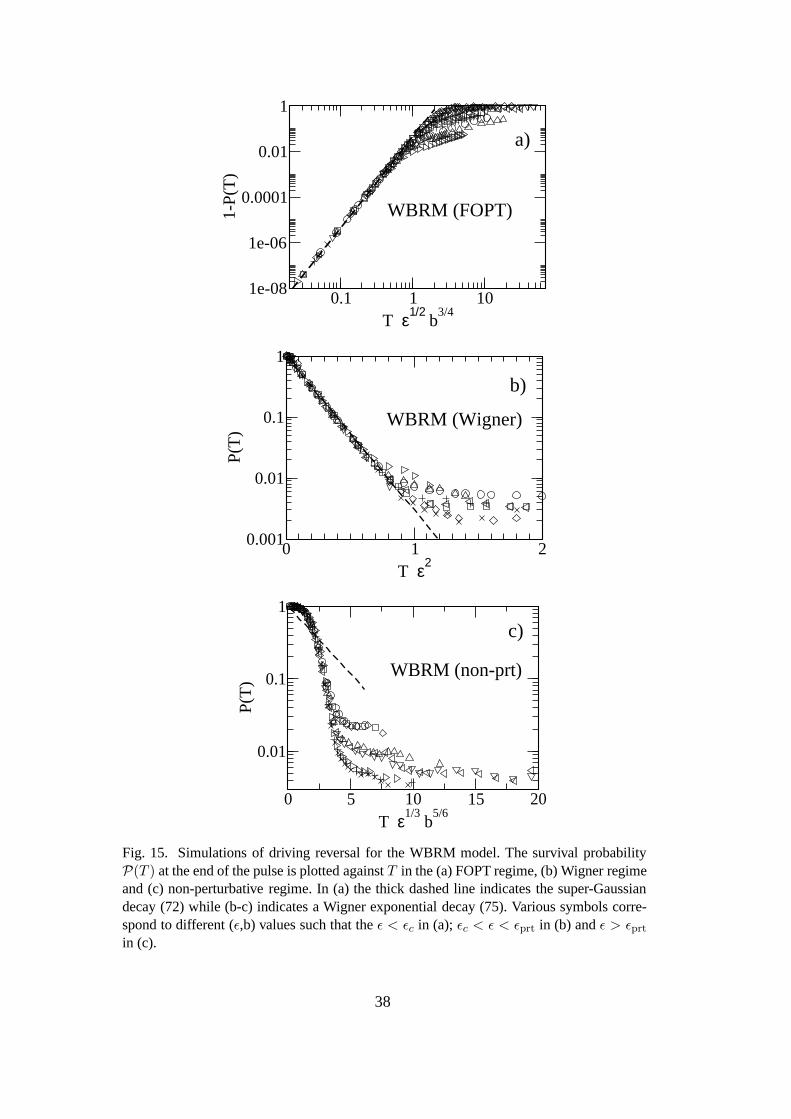
P(T ) ≈ exp(−ε2T 4b3) . (72)

This is a super-Gaussian decay, which is quite different from the standard Gaus-sian decay Eq. (58) or any other results on reversibility that appear in literature[20,21,22,23,24]. We have verified that this expression is valid in the FOPT regime.See Figure 15a.

For the WBRM model, we get the following expression forp(t) after substitutingthe spectral contentFt(ω) given from Eq. (63)

p(t) =(ǫσ)2

∆~×∫ ωcl

−ωcl

dω6 − 4[cos(ωT

2) + cos(ω(T

2− t))] + 2cos(ωt)

ω2. (73)

The corresponding compensation timetPr can be found after minimizing the aboveexpression (corresponding to the maximization ofP(t) = 1− p(t)) with respect totime t. This results in the following equation

si(ωclt) = 2 si(

ωcl

(

t − T

2

))

, (74)

which has to be solved numerically in order to evaluatetPr . Above si(x) =∫ x0

sinxx

.Our numerical data are reported in Fig. 16 together with the theoretical prediction(74).

8.1.4 Decay ofP(t) in the Wigner regime

We now turn to discussP(t) in the ”Wigner regime”. By this we meanεc < ε <εprt. This distinction does not appear in theδE(t) analysis. The time evolution ofδE(t) is dominated by the tails of the distribution and does not affect the ”core”region. ThereforeδE(t) also agreed with LRT outside of the FOPT regime in thewhole (extended) perturbative regime. But this is not the case withP(t), which ismainly influenced by the ”core” dynamics. As a result in the ”Wigner regime” weget different behavior compared with the FOPT regime.

We look at the survival probabilityP(T ) at the end of the driving period. In theWigner regime, instead of the LRT-implied super-Gaussian decay, we find a Wigner-like decay:

P(T ) ≈ e−Γ(ε) T , (75)

36

whereΓ ≈ ε2/∆. In Figure 15b we present our numerical results for various per-turbation strengths in this regime. A nice overlap is observed once we rescale thetime axis asε2×T . We would like to emphasize once more that both in the standardand in the extended perturbative regimes the scaling law involves the perturbationstrengthε. This should be contrasted with the LRT scaling ofδE(t).

What about the compensation timetPr ? A reasonable assumption is that it will ex-hibit a different scaling in the FOPT regime and in the Wignerregime (as is thecase ofP(t)). Namely, in the FOPT regime we would expect ”LRT scaling” withτcl, while in the Wigner regime we would expect ”Wigner scaling”with tprt = ~/Γ.The latter is of non-perturbative nature and reflects the ”core” dynamics. To oursurprise we find that this is not the case. Our numerical data presented in Fig. 16show beyond any doubt that the ”LRT scaling” applies within the whole (extended)perturbative regime, as in the case oftEr , thus not invoking the perturbation strengthε. We see that the FOPT expression (74) fortPr shown as a heavy-dashed line de-scribes the numerical findings.

We conclude that the compensation timetr is mainly related to the dynamics of thetails, and hence can be deduced from the LRT analysis.

8.1.5 Decay ofP(t) in the non-perturbative regime

Let us now turn to the non-perturbative regime (see Fig. 15c). As in the case of thespreading kernelδE(T ), the decay ofP(T ) is no longer captured by perturbationtheory. Instead, we observe the same non-universal scalingwith respect toε1/3 ×Tas in the case ofδE(T ).

P(T ) = hPnprt

(

b5/6ε1/3T)

. (76)

The reason is that in the non-perturbative regime the two energy scalesΓ and∆b,which were responsible for the difference betweenP(T ) and δE(T ), lose theirmeaning. As a consequence, the spreading process involves only one time scaleand the behavior of bothP(T ) andδE(T ) becomes similar, leading to the samescaling behavior.

8.2 Driving Reversal Scenario: 2DW Case

In the representative simulations of the 2DW model in Fig. 12(upper left panel)we see that the spreadingδE(t) for T = 0.48 and various perturbation strengthsε follows the LRT predictions very well. Fig. 12 (lower left panel) shows that theagreement with the LRT is observed for any value of the periodT . This stands inclear contrast to the EBRM model shown in Fig. 12 (right panels).

37

0 1 2T ε2

0.001

0.01

0.1

1

P(T

)

WBRM (Wigner)

0.1 1 10T ε1/2

b3/4

1e-08

1e-06

0.0001

0.01

1

1-P

(T)

WBRM (FOPT)

0 5 10 15 20T ε1/3

b5/6

0.01

0.1

1

P(T

) WBRM (non-prt)

b)

c)

a)

Fig. 15. Simulations of driving reversal for the WBRM model.The survival probabilityP(T ) at the end of the pulse is plotted againstT in the (a) FOPT regime, (b) Wigner regimeand (c) non-perturbative regime. In (a) the thick dashed line indicates the super-Gaussiandecay (72) while (b-c) indicates a Wigner exponential decay(75). Various symbols corre-spond to different (ǫ,b) values such that theǫ < ǫc in (a); ǫc < ǫ < ǫprt in (b) andǫ > ǫprt

in (c).

38

0 10 20 30 T / τ

cl

0.5

0.6

0.7

0.8

0.9

1

t rP / T WBRM (FOPT)

LRT scaling

A

AA

A A

B

BB

B B

0 10 20 30 T / τ

cl

0.5

0.6

0.7

0.8

0.9

1

t rP / T WBRM (Wigner)

LRT scaling

0 5 10 15 20T ε1/3

b5/6

0.5

0.6

0.7

0.8

0.9

1

t rP / T WBRM (non-prt)

c)

b)

a)

Fig. 16. The compensation time is extracted for the same simulations of the previous fig-ures. Note that for both the FOPT regime and the Wigner regimewe have ”LRT scaling”.The thick dashed line corresponds to the LRT prediction Eq. (74) for b = 1. Various sym-bols correspond to different (ǫ,b) values such that theǫ < ǫc in (a); ǫc < ǫ < ǫprt in (b) andǫ > ǫprt in (c).

39

The agreement with LRT in the non-perturbative regime, as inthe case of wavepacketdynamics, reflects detailed QCC. We recall that ”to get into the non-perturbativeregime” and ”to make~ small” means the same. All our simulations are done ina regime where LRT can be trusted at the classical (=non-perturbative) limit. It isonly for RMT models that we observe a breakdown of LRT in the non-perturbativeregime.

What aboutP(T )? This quantity has no classical analogue. Therefore QCC con-siderations are not applicable. Also LDoS considerations cannot help here. Theone-to-one correspondence between the LDoS and the survival probability appliesto the simple wavepacket dynamics scenario (constant perturbation).

It is practically impossible to make a quantitative analysis of P(T ) in the caseof a real model because the band-profile is very structured and there are severenumerical limitations. Rather, what we can easily do is to compare the 2DW withthe corresponding EBRM. Any difference between the two constitutes an indicationfor a non-perturbative effect. Representative simulations are presented in Figure 13.

In Figure 17 we show the dependence of the compensation timetPr on T for theEBRM model. We see very nice scaling behavior that indicatesthat our numerics(as far asP(T ) is concerned!) is limited to the perturbative regime. We emphasizeagain that the physics ofP(t) is very different from the physics ofδE(t). Therefore,this finding by itself should not be regarded as very surprising. A sharp crossover toa non-perturbative behavior can be expected for a “sharp” band-profile only (whichis the WBRM and not the EBRM– see Fig.16).

Now we switch from the EBRM model to the 2DW model. Do we see anydeviationfrom LRT scaling? The answer from Fig. 17 is clearly yes, as reflected by theǫdependence of the curve. The effect is small, but ”it is there”. It indicates that the“body” of the probability distribution, in the case of the 2DW dynamics, does notevolve the same way as in the EBRM case. Indeed we know that themain part ofthe distribution evolves faster (in a ballistic fashion rather than diffusively), andtherefore we observe lower values oftPr .

Assuming that the decay ofP(T ) is given by the exponential law, we extract thecorresponding decay ratesγ. It should be clear that the fitting is done merely inorder to extract a numeric measure for the behavior of the decay. We would notlike to suggest that the decay looks strictly exponential. The results are reportedin Figure 18. We find that forε < εprt, the decay rateγ(ε) ∝ ε2, as expected byWigner’s theory, while forε > εprt we find thatγ ∝ ε. This linear dependence onε is essentially the same as in the corresponding wavepacket dynamics scenario.There it is clearly associated with the widthδEcl ∝ ε of the LDoS.

As far asγ is concerned the behavior of 2DW and the EBRM models are thesame, and there is an indication of the crossover from the perturbative to the non-perturbative regime, as implied (in a non-rigorous fashion) by the LDoS theory. It

40

0 0.2 0.4 0.6 0.8 1 1.2T

0.5

0.6

0.7

0.8

0.9

1

t rP / T

ε = 0.1ε = 0.13ε = 0.16ε = 0.23ε = 0.26ε = 0.29

0 0.2 0.4 0.6 0.8 1 1.2T

0.5

0.6

0.7

0.8

0.9

1

t rP / T

ε = 0.1ε = 0.13ε = 0.16ε = 0.23ε = 0.26ε = 0.29

2DW EBRM

Fig. 17. The compensation timetPr for 2DW simulations, and for the corresponding EBRMsimulations as a function ofT for various values ofε.

0.01 0.1ε

0.1

1

10

γ (ε

)

2DWEBRM

Fig. 18. The estimated decay rateγ for the same simulations as in the previous figure.

is tPr rather thanγ that exhibits sensitivity to the nature of the dynamics. This is be-causetPr is sensitive to the evolution of the main part of the distribution. We alreadyhad made this observation on the basis of the analysis of the WBRM model (seeprevious Subsection 8.1). Here we see another consequence of this observation.

9 Conclusions

There is a hierarchy of challenges in the study of quantum dynamics. The simpleway to explain this hierarchy is as follows: Let us assume that there are two Hamil-tonians,H1 andH2, that differ slightly from each other. Let us then quantify thedifference by a parameterε. Let us distinguish between a FOPT regime, Wignerregime, and non-perturbative (semicircle or semiclassical) regime according to theline shape of the LDoS.Do we have enough information to say something about

41

the dynamics?

In the conventional wavepacket dynamics, one Hamiltonian is used for preparationand for measurement, while the other for propagation. It is well known that theFourier transform of the LDoS gives the survival amplitude and henceP(t). Butwhat about other features of the dynamics. What about the energy spreadingδE(t)for example? It turns out that the answer requires more than just knowing the LDoS.In particular we observe that in the non-perturbative regime physical models differfrom the corresponding RMT model. In the former case we have ballistic spreadingwhile in the latter we have diffusion.

Is there any new ingredient in the study of driving reversal dynamics?Maybe itis just a variation on conventional wavepacket dynamics?The answer turns out tobe interesting. There is a new ingredient in the analysis. This becomes very clearin the RMT analysis where we find a new time scale that distinguishes betweena stage of ”reversible diffusion” and a stage of ”irreversible diffusion”. This timescale (tsdn) can only be probed in a driving reversal experiment. It is absent in thestudy of conventional wavepacket dynamics.

Things become more interesting, and even surprising, once we get into details.Let us summarize our main findings. We start with the conventional wavepacketdynamics, and then turn to the driving reversal scenario.

The main observations regarding wavepacket dynamics are summarized by the di-agrams in Fig. 11. We always have an initial ballistic-like stage which is impliedby FOPT. During this stage the first order (in-band) tails of the energy distribu-tion grow liket2. We call this behavior ”ballistic-like” because the secondmomentδE(t) grows liket2. It is not a genuine ballistic behavior because therth momentdoes not grow liketr but rather all the moments of this FOPT distribution grow liket2.

The bandwidth∆b is resolved at the timeτcl. In the perturbative regime this happensbefore the breakdown of perturbation theory, while in the non-perturbative regimethe breakdowntprt happens beforeτcl. As a result, in the non-perturbative regimewe can get a non-trivial spreading behavior which turns out to be ”ballistic” or”diffusive”, depending on whether the system has a classical limit or is being RMTmodeled.

Once we consider a driving reversal scenario, it turns out tobe important to markthe timetsdn when the energy distribution is resolved. The question is ill-definedin the perturbative regime because there the energy distribution is characterizedby two energy scales (the ”bandwidth” and the much smaller ”core width”). Butthe question is well-defined in the non-perturbative regimewhere the distributionis characterized by one energy scale. It is not difficult to realize that for ballisticbehaviortsdn∼ τcl which is also the classical ergodic time. But for diffusion we getseparation of time scalestprt ≪ tsdn≪ τcl. Thus we conclude that the diffusion has

42

two stages: One is reversible while the other is irreversible.

But the second moment does not fully characterize the dynamics. In the other ex-treme we have the survival probability. WhereasδE(t) is dominated by the tails,P(t) is dominated by the ”core” of the distribution. Therefore itbecomes essentialto distinguish between the FOPT regime where the ”core” is just one level, and therest of the perturbative regime (the ”Wigner” regime) wherethe core is large (butstill smaller compared with the bandwidth).

The main findings regarding the driving reversal scenario are summarized by thefollowing table:

Regime perturbation strength P(T ) behavior tr behavior δE(T ) behavior

1st order perturbative ε < εc LRT LRT LRT

(super-Gaussian) (ballistic-like)

extended perturbative εc < ε < εprt Wigner LRT(!) LRT

(”Wigner”) (Exponential) (ballistic-like)

non-perturbative ε > εprt non-perturbative non-perturbative non-perturbative∗

(non-universal) (non-universal) (diffusive/ballistic)

∗for the WBRM we have diffusion while for the 2DW model we have ballistic behaviour as implied by classical LRT

As expected we find thatP(T ) obeys FOPT behavior in the FOPT regime, whichturns out to be super-Gaussian decay. In the Wigner regimeδE(T ) still obeys LRTbecause the tails obey FOPT, while the non-perturbative core barely affects thesecond moment. But in contrast to thatP(T ) is sensitive to the core, and thereforewe find Wigner (exponential) decay rather than FOPT (super-Gaussian) behavior.However, when we look more carefully at the wholeP(t) curve, we find that thisis not the whole story. We can characterizeP(t) by the compensation timetr. Itturns out thattr is sensitive to the nature of the dynamics. Consequently it obeys”LRT scaling” rather than ”Wigner scaling”. This has further consequences thatare related to quantal-classical correspondence. Just by looking atP(T ) we cannottell whether we look at the ”real simulation” or on its RMT modeling. But lookingon tr we can find a difference. It turns out that in the physical model tr exhibitsεdependence, while in the case of RMT modelingtr is independent ofε and exhibits”Wigner scaling”.

Finally we come to the non-perturbative regime. Here we have, in a sense a simplersituation. We have only one energy scale, and hence only one time scale, and there-fore δE(T ) andP(t) essentially obeys the same scaling. Indeed we have verifiedthat the non-perturbative scaling withtsdn in WBRM simulations is valid for boththe second moment and the survival probability.

43

Finally we would like to emphasize that the notion of ”non-perturbative” behaviorshould not be confused with ”non-linear” response. In case of quantized models,linear response of the energy spreadingδE(T ) is in fact a consequence of non-perturbative behavior. This should be contrasted with the WBRM model, whereQCC does not apply, and indeed deviations from the linear response appear oncewe enter the non-perturbative regime.

The study of irreversibility in a simple driving reversal scenario is an important steptowards the understanding of irreversibility and dissipation in general. The analysisof dissipation reduces to the study of energy spreading for time dependent Hamil-toniansH(Q, P ; x(t)). In generic circumstances the rate of energy absorption isdetermined by a diffusion-dissipation relation: The long time process of dissipationis determined by the short time diffusion process. The latter is related to the fluctu-ationsC(ω) via what we call ”LRT formula”. Thus the understanding of short timedynamics is the crucial step in establishing the validity ofthe fluctuation-dissipationrelation.

Acknowledgments

This research was supported by a grant from the GIF, the German-Israeli Founda-tion for Scientific Research and Development, and by the Israel Science Foundation(grant No.11/02).

References

[1] M. Wilkinson, J. Phys. A20 (1987) 2415.

[2] M. Wilkinson, J. Phys. A21 (1988) 4021.

[3] M. Wilkinson, E. Austin,J. Phys. A28 (1995) 2277.

[4] A. Bulgac, G. D. Dang, D. Kusnezov,Phys. Rev. E54 (1996) 3468.

[5] U. Weiss,Quantum Dissipative Systems, World Scientific, 1998.

[6] M. Wilkinson, Parametric Random Matrices: Static and Dynamic Applications, pp.369-399, Kluwer Academic / Plenum Publishers, New York, 1999.

[7] D. Cohen,Ann. Phys.283 (2000) 175.

[8] D. Cohen, T. Kottos,Phys. Rev. Lett.85 (2000) 4839.

44

[9] D. Wisniacki, D. Cohen,Phys. Rev. E66 (2002) 046209.

[10] T. Kottos, D. Cohen,Europhys. Lett.61 (2003) 431.

[11] D. Cohen, T. Kottos,J. Phys. A36 (2003) 10151.

[12] E. Wigner,Ann. Math.62 (1955) 548.

[13] E. Wigner,Ann. Math.65 (1957) 203.

[14] H.-J. Stockmann,Quantum Chaos: an introduction, University Press, Cambridge,1998.

[15] F. Haake,Quantum Signatures of Chaos, 2nd Edition, Springer-Verlag, Berlin,Heidelberg, New York, 2000.

[16] Y. Alhassid,Rev. Mod. Phys.72 (2000) 895.

[17] D. Cohen, F. Izrailev, T. Kottos,Phys. Rev. Lett.84 (2000) 2052.

[18] T. Kottos, D. Cohen,Phys. Rev. E64 (2001) 0652021.

[19] D. Cohen, T. Kottos,Phys. Rev. E63 (2001) 036203.

[20] T. Prosen, T. H. Seligman,J. Phys. A35 (2002) 4707.

[21] G. Benenti, G. Casati,Phys. Rev. E66 (2002) 066205.

[22] R. Jalabert, H. Pastawski,Phys. Rev. Lett.86 (2001) 2490.

[23] C. B. Ph. Jacquod, I. Adagideli,Phys. Rev. Lett.89 (2002) 154103.

[24] M. Hiller, T. Kottos, D. Cohen, T. Geisel,Phys. Rev. Lett.92 (2004) 010402.

[25] R. A. Pullen, A. R. Edmonds,J. Phys. A14 (1981) L477.

[26] H. D. Meyer,J. Chem. Phys.84 (1986) 3147.

[27] O. Bohigas, M. Giannoni, C. Schmidt,Phys. Rev. Lett.52 (1984) 1.

[28] M. Berry,Chaos and Quantum Systems, Elsevier, 1991.

[29] Y. Imry, Introduction to Mesoscopic Physics, Oxford University Press, New York,Oxford, 1997.

[30] M. Berry, J. Phys. A10 (1977) 2083.

[31] T. Prosen, M. Robnik,J. Phys. A26 (1993) L319.

[32] T. Prosen,Ann. Phys.235 (1994) 115.

[33] E. Austin, M. Wilkinson,Nonlinearity5 (1992) 1137.

[34] M. Feingold, D. Leitner, M. Wilkinson,Phys. Rev. Lett.66 (1991) 986.

[35] M. Feingold, A. Gioletta, F. Izrailev, L. Molinari,Phys. Rev. Lett.70 (1993) 2936.

[36] Y. Fyodorov, O. Chubykalo, F. Izrailev, G. Casati,Phys. Rev. Lett.76 (1996) 1603.

45

[37] F. Izrailev, T. Kottos, A. Politi, G. Tsironis,Phys. Rev. E55 (1997) 4951.

[38] J. A. Mendez-Bermudez, T. Kottos, D. Cohen, submitted 2004.

[39] F. Borgonovi, I. Guarneri, F. Izrailev,Phys. Rev. E57 (1998) 5291.

46