waves in the atmosphere and oceanswaves ... - …yu/class/ess228/lecture.6.adjustment.all.pdf ·...

Waves in the Atmosphere and OceansWaves in the Atmosphere and OceansWaves in the Atmosphere and OceansWaves in the Atmosphere and OceansRestoring Force

Conservation of potential temperature in the presence of positive static stability internal gravity waves

Conservation of potential vorticity in the presence of a mean gradient of potential vorticity Rossby waves

• External gravity wave (Shallow-water gravity wave) • Internal gravity (buoyancy) wave• Inertial-gravity wave: Gravity waves that have a large enough

wavelength to be affected by the earth’s rotation.• Rossby Wave: Wavy motions results from the conservation of potentialRossby Wave: Wavy motions results from the conservation of potential

vorticity.• Kelvin wave: It is a wave in the ocean or atmosphere that balances the

C i li f i t t hi b d h tliESS228Prof. Jin-Yi Yu

Coriolis force against a topographic boundary such as a coastline, or a waveguide such as the equator. Kelvin wave is non-dispersive.

Lecture 6: Adjustment under Gravity Lecture 6: Adjustment under Gravity in a Nonin a Non--Rotating SystemRotating Systemin a Nonin a Non--Rotating SystemRotating System

• Overview of Gravity waves• Surface Gravity Wavesy• “Shallow” Water• Shallow-Water Model

ESS228Prof. Jin-Yi Yu

• Dispersion

Goals of this ChapterGoals of this Chapterpp• This chapter marks the beginning of more detailed study of the way the

atmosphere-ocean system tends to adjust to equilibrium.

• The adjustment processes are most easily understood in the absence of driving forces. Suppose, for instance, that the sun is "switched off," leaving the atmosphere and ocean with some non-equilibrium distribution of p qproperties.

• How will they respond to the gravitational restoring force?

• Presumably there will be an adjustment to some sort of equilibrium. If so, what is the nature of the equilibrium?

• In this chapter, complications due to the rotation and shape of the earth will p , p pbe ignored and only small departures from the hydrostatic equilibrium will be considered.

• The nature of the adjustment processes will be found by deduction from the


j p yequations of motion

Gravity WavesGravity Waveshttp://skywarn256.wordpress.com

• Gravity waves are waves generated in a fluid medium or at the interface between

http://www.astronautforhire.com

two media (e.g., the atmosphere and the ocean) which has the restoring force of gravity or buoyancy.

• When a fluid element is displaced on an interface or internally to a region with a• When a fluid element is displaced on an interface or internally to a region with a different density, gravity tries to restore the parcel toward equilibrium resulting in an oscillation about the equilibrium state or wave orbit.


• Gravity waves on an air-sea interface are called surface gravity waves or surface waves while internal gravity waves are called internal waves.

Adjustment Under Gravity in aAdjustment Under Gravity in aAdjustment Under Gravity in a Adjustment Under Gravity in a NonNon--Rotating SystemRotating System

External Gravity Waves Internal Gravity Wavesadjustment of a homogeneous fluid

with a free surfaceadjustment of a density-stratified

fluid


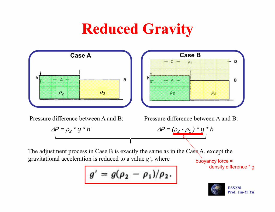
Reduced GravityReduced GravityCase A Case B

ρ2 ρ2

Pressure difference between A and B: Pressure difference between A and B:

ρ2 ρ2

Pressure difference between A and B:

ΔP = ρ2 * g * h

Pressure difference between A and B:

ΔP = (ρ2 - ρ1 ) * g * h

The adjustment process in Case B is exactly the same as in the Case A, except the gravitational acceleration is reduced to a value g’, where buoyancy force =

density difference * g


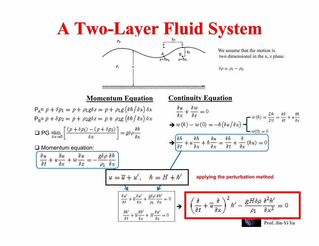
A TwoA Two--Layer Fluid SystemLayer Fluid SystemWe assume that the motion istwo dimensional in the x, z plane.

Momentum EquationP

Continuity EquationPA=PB=

PG =

Momentum equation:

applying the perturbation method


Shallow Water Gravity WaveShallow Water Gravity WaveWe assume that the motion istwo dimensional in the x, z plane.

Governing EquationSh ll i lShallow water gravity waves may also occur at thermocline where the surface water is separated from the deep water. (These waves can also referred to as the internal gravity waves).

If the density changes by an amount δρ/ρ1 ≈ 0.01, across the thermocline, then the wave speed for waves traveling along the thermocline will be only one tenth of the surface wave speed for a fluid of

(e.g., air and water)one-tenth of the surface wave speed for a fluid of the same depth.

The shallower the water, the slower the wave.Shallo ater gra it a es are non dispersi e

ESS228Prof. Jin-Yi YuShallow water wave speed ≈ 200 ms-1 for an ocean depth of 4km

Shallow water gravity waves are non-dispersive.

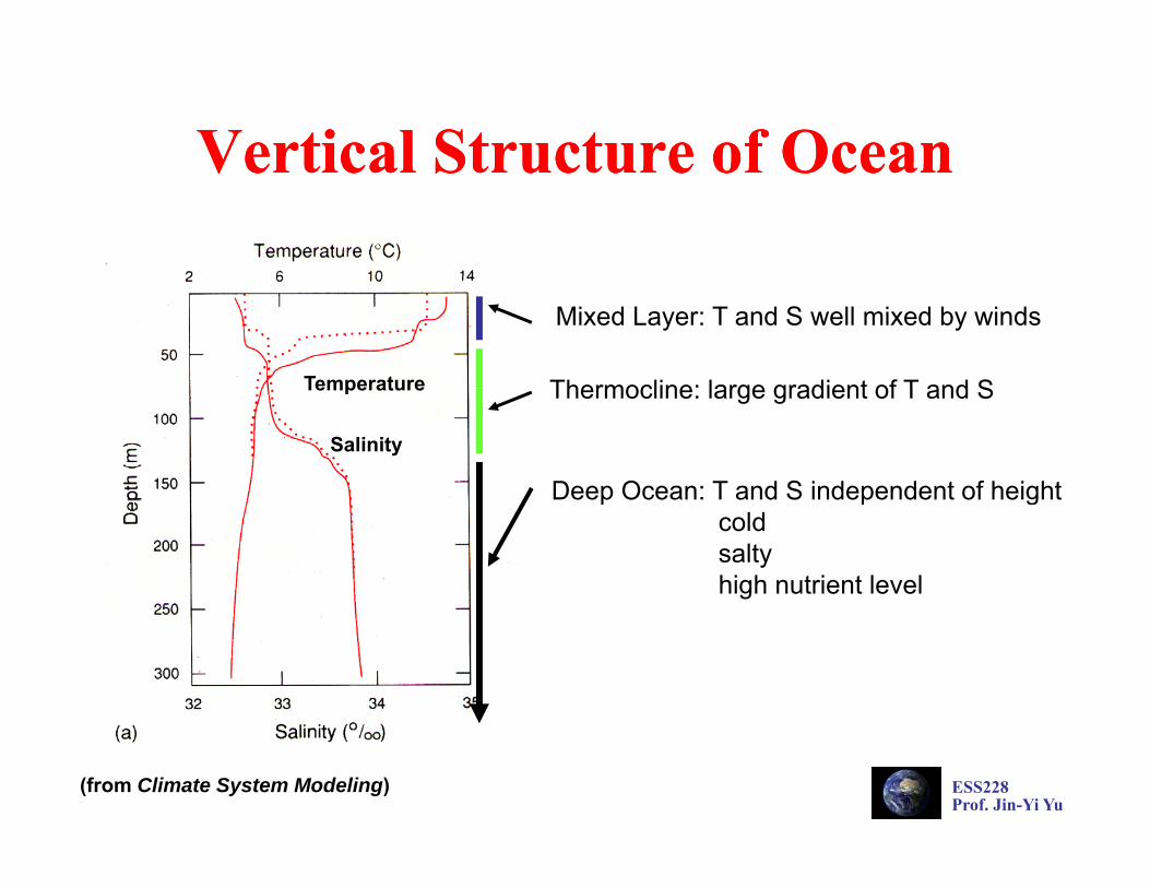
Vertical Structure of OceanVertical Structure of OceanVertical Structure of OceanVertical Structure of Ocean

Temperature

Mixed Layer: T and S well mixed by winds

Thermocline: large gradient of T and STemperature

Salinity

Thermocline: large gradient of T and S

Deep Ocean: T and S independent of height p p gcoldsaltyhigh nutrient level


(from Climate System Modeling)

Shallow and Deep WaterShallow and Deep WaterShallow and Deep WaterShallow and Deep Water• “Shallow” in this lecture means that the depth of the fluid layer

is small compared with the horizontal scale of the perturbation, i.e., the horizontal scale is large compared with the vertical scale.scale.

• Shallow water gravity waves are the ‘long wave approximation” end of gravity waves.

• Deep water gravity waves are the “short wave approximation” end of gravity waves.

• Deep water gravity waves are not important to large-scale motions in the oceans.


Internal Gravity (Buoyancy) WavesInternal Gravity (Buoyancy) Waves

In a fluid, such as the ocean, which is bounded both above and below, gravity waves propagate primarily in the horizontal plane since vertically traveling waves are reflected from the boundaries to form standing waves.

In a fluid that has no upper boundary, such as the atmosphere, gravity waves may propagate vertically as well as horizontally. In vertically propagating waves the phase is a function of height. Such waves are referred to as internal waves.

Although internal gravity waves are not generally of great importance for synoptic-scale weather forecasting (and indeed are nonexistent in the filtered quasi-geostrophic models), they can be important in mesoscale motions.

For example they are responsible for the occurrence of mountain lee waves They also are believed to


For example, they are responsible for the occurrence of mountain lee waves. They also are believed to be an important mechanism for transporting energy and momentum into the middle atmosphere, and are often associated with the formation of clear air turbulence (CAT).

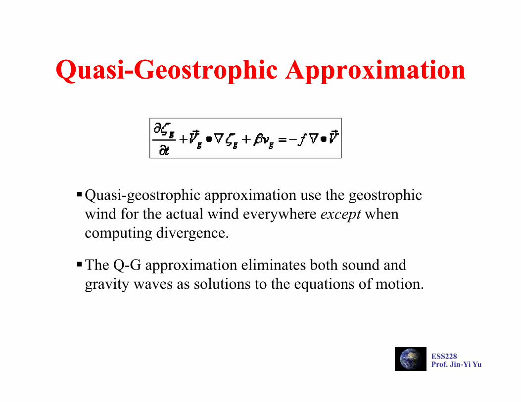
QuasiQuasi--GeostrophicGeostrophic ApproximationApproximationQuasiQuasi GeostrophicGeostrophic ApproximationApproximation

Quasi-geostrophic approximation use the geostrophic wind for the actual wind everywhere except when computing divergence.

The Q-G approximation eliminates both sound and gravity waves as solutions to the equations of motion.


Lecture 7: Adjustment under Gravity Lecture 7: Adjustment under Gravity of a Densityof a Density Stratified FluidStratified Fluidof a Densityof a Density--Stratified FluidStratified Fluid

• Normal Mode & Equivalent Depth• Rigid Lid Approximation• Boussinesq Approximation• Buoyancy (Brunt-Väisälä ) Frequency


• Dispersion of internal gravity waves

Main Purpose of This LectureMain Purpose of This LectureMain Purpose of This LectureMain Purpose of This Lecture• As an introduction to the effects of stratification, the

f d h ll l h fcase of two superposed shallow layers, each of uniform density, is considered.

• In reality, both the atmosphere and ocean are continuously stratified.

• This serves to introduce the concepts of barotropicand baroclinic modes.

• This also serves to introduce two widely used approximations: the rigid lid approximation and the


Boussinesq approximation.

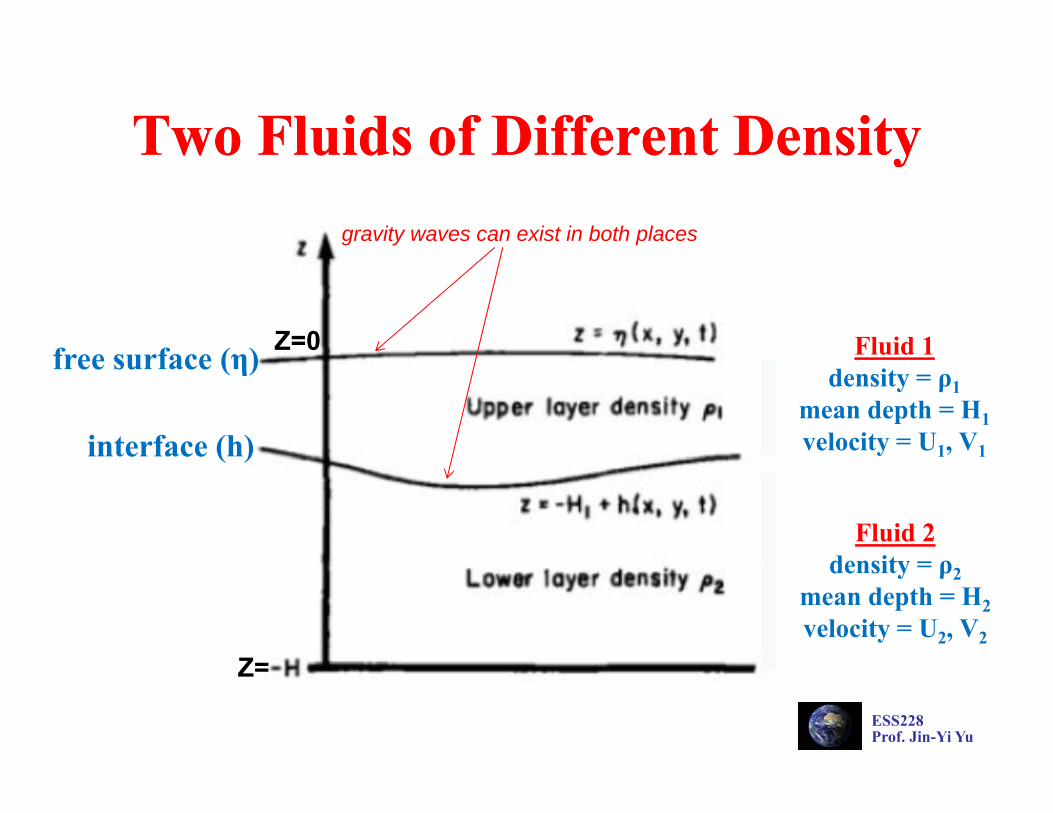
Two Fluids of Different DensityTwo Fluids of Different DensityTwo Fluids of Different DensityTwo Fluids of Different Densitygravity waves can exist in both places

Fluid 1free surface (η) Z=0density = ρ1

mean depth = H1velocity = U1, V1

free surface (η)

interface (h)

Fluid 2d it

( )

density = ρ2mean depth = H2velocity = U2, V2

Z=


Z=

Two Fluids: Two Fluids: Layer 1Layer 1 ( )( )

P0 = 0 M t E tiP0 0

P

Momentum Equations

P1

PContinuity Equation

P2

Taking time derivative of the continuity equation:


Two Fluids: Two Fluids: Layer 2Layer 2 ( )( )

Momentum Equations

P0 = 0

P1 = reduced gravityContinuity Equation

P2

g y

Taking time derivative of the continuity


equation:

Adjustments of the TwoAdjustments of the Two--Fluid SystemFluid SystemThe adjustments in the two-layer fluid system are governed by:

Combined these two equations will result in a fourth-order qequation, which is difficult to solve.This problem can be greatly simplified by looking for solutions

which η and h are proportional:

i i i iThe governing equations will both reduced to this form:provided that There are two values of μ (and hence two

values of c ) that satisfy this equation


values of ce) that satisfy this equation.The motions corresponding to these particular vales are called normal modes of oscillation.

Normal ModesNormal ModesNormal ModesNormal Modes

barotropic mode baroclinic mode

• The motions corresponding to these particular values of ce or μ are called normal modes of oscillation.

p

• In a system consisting of n layers of different density, there are n normal modes corresponding to the n degrees of freedom.


• A continuously stratified fluid corresponding to an infinite number of layers, and so there is an infinite set of modes.

Structures of the Normal ModesStructures of the Normal ModesThe structures of the normal modes can be obtained by solving this equation (from previous slide):

Or, we can use the concept of the one-layer shallow water model, where the phase speed (c) of the gravity wave is related to the depth of the shallow water (H):

Using this concept, we can assume each of the normal mode behaves like the one-layer shallow water with a “equivalent depth” of He:

Solution 1(brotropic mode)


Solution 2(baroclinic mode)

Structures of the Normal ModesStructures of the Normal Modes

free surface (η)

i t f (h)H1interface (h)

H2

H=H1+H2

Barotropic mode Baroclinic mode


η>h ; u2&u1 of same signs η<h ; u2&u1 of opposite signs

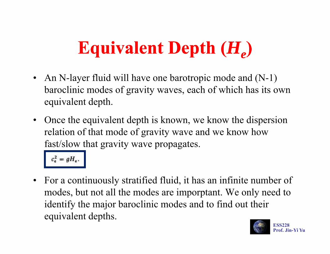
Equivalent Depth (Equivalent Depth (HH ))Equivalent Depth (Equivalent Depth (HHee))• An N-layer fluid will have one barotropic mode and (N-1)An N-layer fluid will have one barotropic mode and (N-1)

baroclinic modes of gravity waves, each of which has its own equivalent depth.

• Once the equivalent depth is known, we know the dispersion relation of that mode of gravity wave and we know how fast/slow that gravity wave propagatesfast/slow that gravity wave propagates.

• For a continuously stratified fluid, it has an infinite number of modes, but not all the modes are imporptant. We only need to identify the major baroclinic modes and to find out their


identify the major baroclinic modes and to find out their equivalent depths.

Rigid Lid ApproximationRigid Lid Approximation(for the upper layer)(for the upper layer)(for the upper layer)(for the upper layer)

Momentum Equationsη

hContinuity Equation

h

• For baroclinic modes surface displacements (η)• For baroclinic modes, surface displacements (η) are small compared to interface displacements (h).

• If there is a rigid lid at z=0, the identical pressure gradients would have be achieved.


Purpose of Rigid Lid ApproximationPurpose of Rigid Lid Approximationp g ppp g pp• Rigid lid approximation: the upper surface was held fixed but

ld h l d f lcould support pressure changes related to waves of lower speed and currents of interest.

• Ocean models used the "rigid lid" approximation to eliminate• Ocean models used the rigid lid approximation to eliminate high-speed external gravity waves and allow a longer time step.

• As a result, ocean tides and other waves having the speed of tsunamis were filtered out. Th i id lid i i d i h 70' fil• The rigid lid approximation was used in the 70's to filter out gravity wave dynamics in ocean models. Since then, ocean model have evolved to include a free-surface allowing fast-


gmoving gravity wave physics.

BoussinesqBoussinesq ApproximationApproximation(for the lower layer)(for the lower layer)(for the lower layer)(for the lower layer)

Momentum Equationsη

hh

Continuity Equation

• Boussinesq approx: replace the ratio (ρ1/ρ2) by unity in the momentum equation.

• We keep the density difference in this


We keep the density difference in this g′ term, because it involves density difference (ρ1- ρ2)/ ρ1*g, which is related to the buoyancy force.

Purpose of Purpose of BoussinesqBoussinesq ApproximationApproximation• This approximation states that density differences are sufficiently small to

be neglected, except where they appear in terms multiplied by g, the acceleration due to gravity (i.e., buoyancy).

• In the Boussinesq approximation, which is appropriate for an almost-incompressible fluid, it assumed that variations of density are small, so that in the intertial terms, and in the continuity equation, we may substitute ρ byρ0, a constant. However, even weak density variations are important in buoyancy, and so we retain variations in ρ in the buoyancy term in the vertical equation of motion.

• Sound waves are impossible/neglected when the Boussinesq approximation is used, because sound waves move via density variations.

• Boussinesq approximation is for the problems that the variations ofBoussinesq approximation is for the problems that the variations of temperature as well as the variations of density are small. In these cases, the variations in volume expansion due to temperature gradients will also small. For these case, Boussinesq approximation can simplify the problems


, q pp p y pand save computational time.

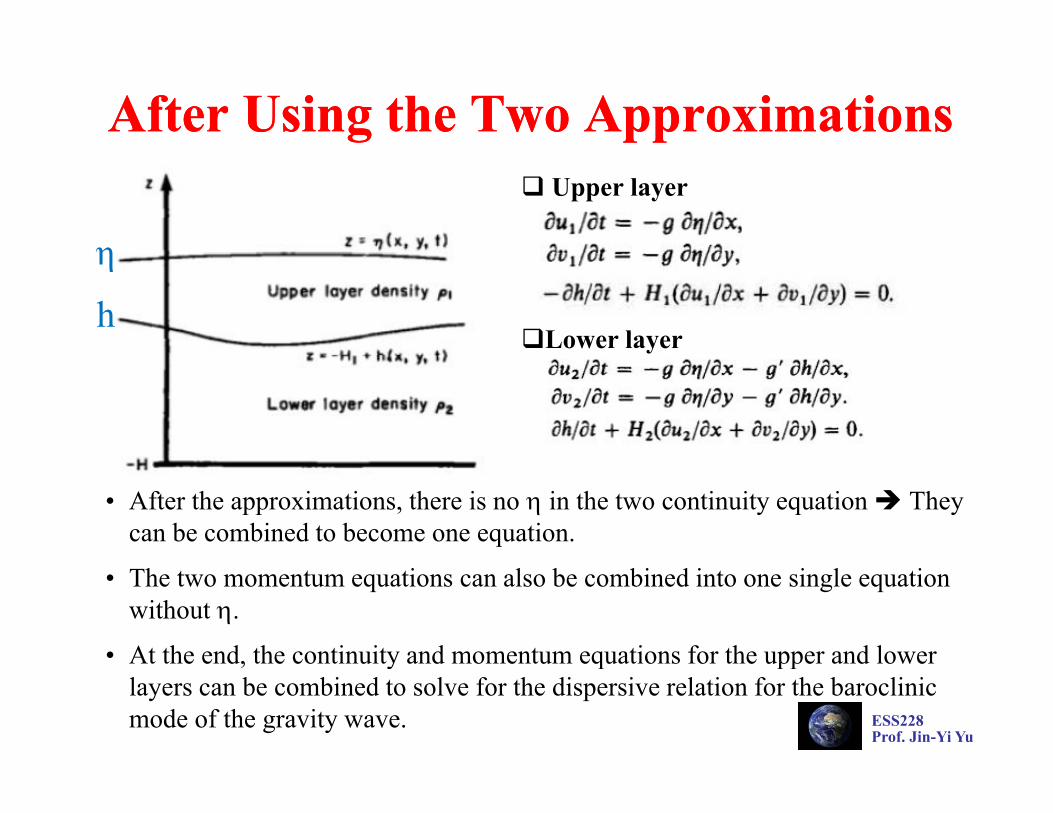
After Using the Two ApproximationsAfter Using the Two ApproximationsUpper layer

η

Lower layer

η

h

• After the approximations, there is no η in the two continuity equation They can be combined to become one equation.

• The two momentum equations can also be combined into one single equation without η.

• At the end, the continuity and momentum equations for the upper and lower


At the end, the continuity and momentum equations for the upper and lower layers can be combined to solve for the dispersive relation for the baroclinic mode of the gravity wave.

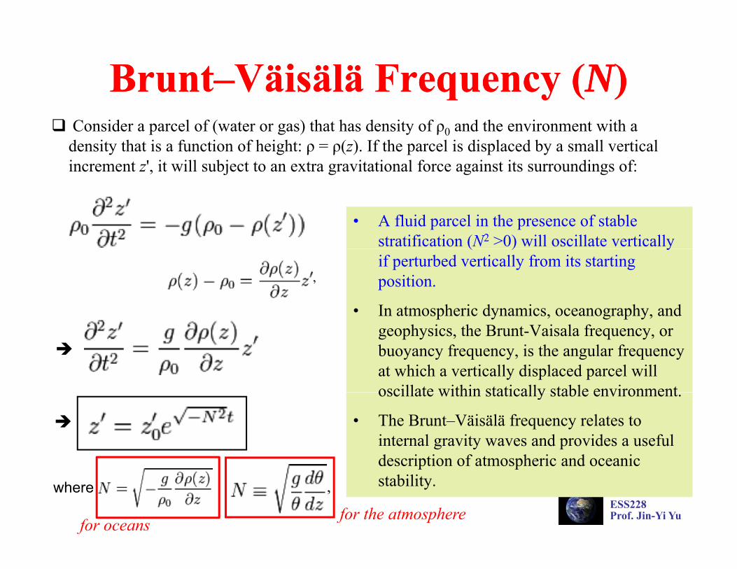
BruntBrunt––VäisäläVäisälä Frequency (Frequency (NN))Consider a parcel of (water or gas) that has density of ρ0 and the environment with a density that is a function of height: ρ = ρ(z). If the parcel is displaced by a small vertical increment z', it will subject to an extra gravitational force against its surroundings of:

• A fluid parcel in the presence of stable stratification (N2 >0) will oscillate vertically ( ) yif perturbed vertically from its starting position.

• In atmospheric dynamics, oceanography, and geophysics, the Brunt-Vaisala frequency, or buoyancy frequency, is the angular frequency at which a vertically displaced parcel will oscillate within statically stable environmentoscillate within statically stable environment.

• The Brunt–Väisälä frequency relates to internal gravity waves and provides a useful description of atmospheric and oceanic


description of atmospheric and oceanic stability.where

for the atmospherefor oceans

Internal Gravity Waves in Atmosphere and OceansInternal Gravity Waves in Atmosphere and Oceanshttp://skywarn256.wordpress.com

In AtmosphereIn Oceans

Internal gravity waves can be found in both the statically stable (dӨ/dz>0) atmosphere and the stably stratified (-dρ/dz>0)ocean.and the stably stratified ( dρ/dz 0)ocean.

The buoyancy frequency for the internal gravity wave in the ocean is determined by the vertical density gradient, while it is determined by the vertical gradient of potential temperature.p

In the troposphere, the typical value of N is 0.01 sec-1, which correspond to a period of about 10 minutes.

Although there are plenty of gravity waves in the atmosphere most of them have smallAlthough there are plenty of gravity waves in the atmosphere, most of them have small amplitudes in the troposphere and are not important, except that the gravity waves generated by flows over mountains. These mountain waves can have large amplitudes.

Gravity waves become more important when they propagate into the upper atmosphere


Gravity waves become more important when they propagate into the upper atmosphere (particularly in the mesosphere) where their amplitudes got amplified due to low air density there.

Dispersion of Internal Gravity WavesDispersion of Internal Gravity Wavesmean flow zonal wavenumber vertical wavenumber total wavenumber

Phase velocity:

is always smaller than N!! Internal gravity waves can have any frequency between zero and a maximum value of N.

Group velocity:

Internal gravity waves thus have the remarkable In the atmosphere, internal gravity waves generated in the troposphere by cumulus

(from H.-C. Kuo, National Taiwan Univ.)


property that group velocity is perpendicular to the direction of phase propagation.

generated in the troposphere by cumulus convection, by flow over topography, and by other processes may propagate upward many scale heights into the middle atmosphere.

Kelvin WavesKelvin WavesGoverning Equations

Y

X A unique boundary condition

• A Kelvin wave is a type of low-frequency gravity wave in the ocean or atmosphere that balances the Earth's Coriolis force against a topographic boundary such as a coastline, or a waveguide such as the equator.

• Therefore, there are two types of Kelvin waves: coastal and equatorial.

• A feature of a Kelvin wave is that it is non-dispersive, i.e., the phase speed of the wave crests is equal to the group speed of the wave energy for all


of the wave crests is equal to the group speed of the wave energy for all frequencies.

Costal Kelvin WavesCostal Kelvin Waves• Coastal Kelvin waves always

propagate with the shoreline on the right in the northernA h the right in the northern hemisphere and on the left in the southern hemisphere.

• In each vertical plane to the

At the coast

• In each vertical plane to the coast, the currents (shown by arrows) are entirely within the plane and are exactly the same

depth of the fluid

plane and are exactly the same as those for a long gravity wave in a non-rotating channel.

• However the surface elevation• However, the surface elevation varies exponentially with distance from the coast in order to give a geostrophic balance.


to give a geostrophic balance.

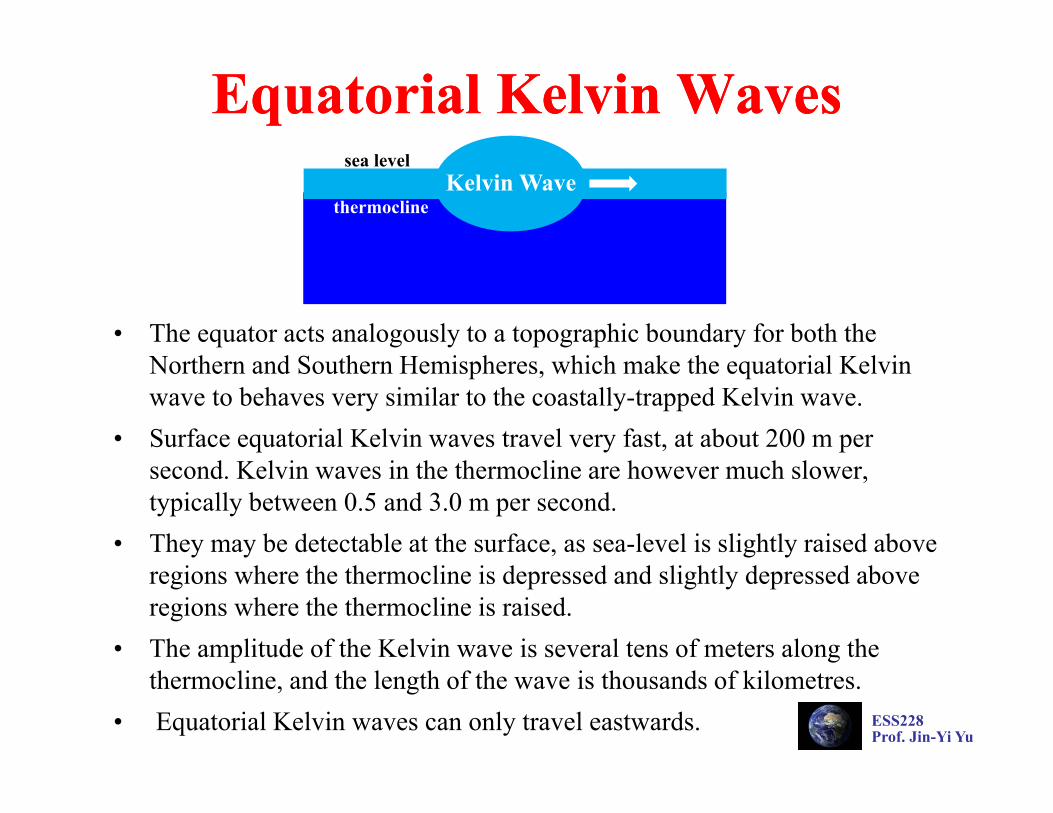
Equatorial Kelvin WavesEquatorial Kelvin Waves

thermocline

sea levelKelvin Wave

• The equator acts analogously to a topographic boundary for both the h d h i h hi h k h i l l iNorthern and Southern Hemispheres, which make the equatorial Kelvin

wave to behaves very similar to the coastally-trapped Kelvin wave.• Surface equatorial Kelvin waves travel very fast, at about 200 m per

second. Kelvin waves in the thermocline are however much slower, typically between 0.5 and 3.0 m per second.

• They may be detectable at the surface, as sea-level is slightly raised above regions where the thermocline is depressed and slightly depressed above regions where the thermocline is raised.

• The amplitude of the Kelvin wave is several tens of meters along the


thermocline, and the length of the wave is thousands of kilometres.• Equatorial Kelvin waves can only travel eastwards.

19971997--98 El Nino98 El Nino19971997 98 El Nino98 El Nino


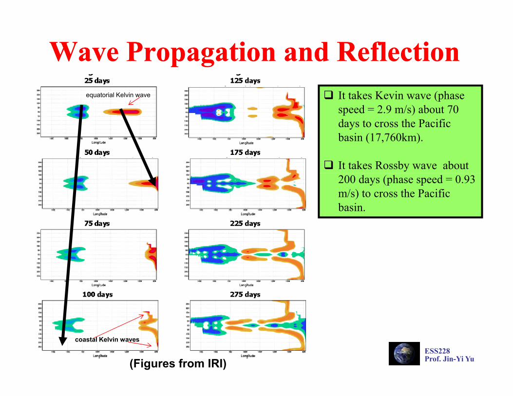
Wave Propagation and ReflectionWave Propagation and ReflectionIt takes Kevin wave (phase speed = 2.9 m/s) about 70 days to cross the Pacific

equatorial Kelvin wave

days to cross the Pacific basin (17,760km).

It takes Rossby wave about 200 days (phase speed = 0.93 m/s) to cross the Pacific basin.

ESS228Prof. Jin-Yi Yu(Figures from IRI)

coastal Kelvin waves

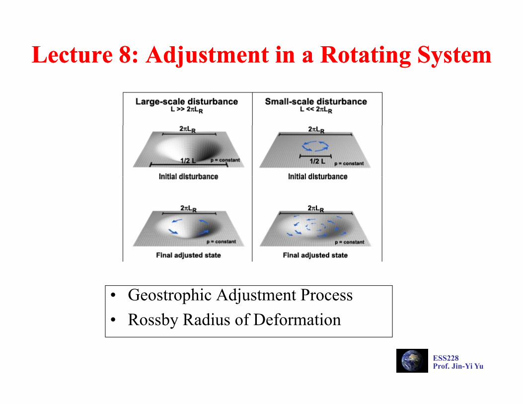
Lecture 8: Adjustment in a Rotating SystemLecture 8: Adjustment in a Rotating System

• Geostrophic Adjustment Process• Rossby Radius of Deformation


Geostrophic AdjustmentsGeostrophic Adjustments

• The atmosphere is nearly always close to geostrophic and hydrostatic balancebalance.

• If this balance is disturbed through such processes as heating or cooling, the atmosphere adjusts itself to get back into balance. This process is called

t hi dj t tgeostrophic adjustment.• A key feature in the geostrophic adjustment process is that pressure and

velocity fields have to adjust to each other in order to reach a geostrophic balance When the balance is achie ed the flo at an le el is along thebalance. When the balance is achieved, the flow at any level is along the isobars.

• We can study the geostrophic adjustment by studying the adjustment in a b i fl id i h h ll ibarotropic fluid using the shallow-water equations.

• The results can be extended to a baroclinic fluid by using the concept of equivalent depth.


Geostrophic Adjustment ProblemGeostrophic Adjustment Problemshallow water model

If we know the distribution of perturbation potential vorticity (Q’) at the initial time, we know for all time:


And the final adjusted state can be determined without solving the time-dependent problem.

An Example of Geostrophic AdjustmentAn Example of Geostrophic AdjustmentFinal Adjusted StateInitial Perturbed State

motionless (u=0 and v=0)

Transient


Inertial-gravity waves

Final Adjusted StateFinal Adjusted StateFinal Adjusted State Radius of deformation:

•The steady equilibrium solution is not one of rest, but is a geostrophic balance.

•The equation determining this steady solution contains a length scale a, called the Rossby radius of deformation.

•The energy analysis indicates that energy is hard to extract from a rotating fluid. In the problem studied, there was an infinite amount of potential energy available for conversion into kinetic energy, but only a finite amount of this available energy


for conversion into kinetic energy, but only a finite amount of this available energy was released. The reason was that a geostrophic equilibrium was established, and such an equilibrium retains potential energy.

Rossby Radius of DeformationRossby Radius of DeformationFor Barotropic Flow For Baroclinic Flow

Brunt-Vaisala frequency

equivalent depthwater depth

• In atmospheric dynamics and physical oceanography, the Rossby radius of deformation is the length scale at which rotational effects become as important as buoyancy or gravity wave effects in the evolution of the flowimportant as buoyancy or gravity wave effects in the evolution of the flow about some disturbance.

• “deformation”: It is the radius that the direction of the flow will be “deformed” by the Coriolis force from straight down the pressure gradient todeformed by the Coriolis force from straight down the pressure gradient to be in parallel to the isobars.

•The size of the radius depends on the stratification (how density or potential h i h h i h ) d C i li


temperature changes with height) and Coriolis parameter.

• The Rossby radius is considerably larger near the equator.

Rossby Radius and the Equilibrium StateRossby Radius and the Equilibrium StateM d V l it E P titiMass and Velocity Energy Partition

• For large scales (KHa « 1), the potential vorticity perturbation is mainly associated with

water number deformation radius

For large scales (KHa « 1), the potential vorticity perturbation is mainly associated with perturbations in the mass field, and that the energy changes are in the potential and internal forms.

• For small scales (KHa » 1) potential vorticity perturbations are associated with the velocity field, and the energy perturbation is mainly kinetic.

• At large scales (KH-1 » a; or KHa « 1), it is the mass field that is determined by the initial

potential vorticity, and the velocity field is merely that which is in geostrophic equilibrium with the mass field It is said therefore that the large scale velocity field adjusts to be inwith the mass field. It is said, therefore, that the large-scale velocity field adjusts to be in equilibrium with the large scale mass field.

• At small scales (KH-1 « a) it is the velocity field that is determined by the initial potential

vorticity, and the mass field is merely that which is in geostrophic equilibrium with the


y, y g p qvelocity field. In this case it can be said that the mass field adjusts to be in equilibrium with the velocity field.

Rossby Radius and the Equilibrium StateRossby Radius and the Equilibrium State• If the size of the disturbance is much larger than the Rossby

di f d f i h hradius of deformation, then the velocity field adjusts to the initial mass (height) field.

• If the size of the disturbance is much smaller than the Rossby radius of deformation, then the

fi ld dj h i i i lmass field adjusts to the initial velocity field.

• If the size of the disturbance is close to the Rossby radius of deformation, then both the velocity and mass fields undergo

l dj


mutual adjustment.

What does the Geostrophic Adjustment Tell Us?What does the Geostrophic Adjustment Tell Us?What does the Geostrophic Adjustment Tell Us?What does the Geostrophic Adjustment Tell Us?

• An important feature of the response of a rotating ftuid to gravity is that it does not adjust to a state of rest, but rather to a geostrophic equilibrium.

• The Rossby adjustment problem explains why the atmosphere and ocean are nearly always close to geostrophic equilibrium for if any force tries toare nearly always close to geostrophic equilibrium, for if any force tries to upset such an equilibrium. the gravitational restoring force acts quickly to restore a near-geostrophic equilibrium.

• For deep water in the ocean, where H is 4 or 5 km. c is about 200 m/s and therefore the Rossby radius a = c/f ~ 2000 km.

• Near the continental shelves, such as for the North Sea where H=40m, theNear the continental shelves, such as for the North Sea where H 40m, the Rossby radius a = c/f ~ 200 km. Since the North Sea has larger dimensions than this, rotation has a strong effect on transient motions such as tides and surges in that ocean region.


Lecture 9: Tropical DynamicsLecture 9: Tropical Dynamics

• Equatorial Beta PlaneEquatorial Beta Plane• Equatorial Wave Theory• Equatorial Kelvin Wavequato a e v Wave• Adjustment under Gravity near the Eq.• Gill Type Response


yp p

OverviewOverviewOverviewOverview

•In the Mid-latitudes, the primary energy source for synoptic-scale disturbances is the zonal available potential energy associated with thedisturbances is the zonal available potential energy associated with the latitudinal temperature gradient; and latent heat release and radiative heating are usually secondary contributors.

•In the tropics, however, the storage of available potential energy is small due to the very small temperature gradients in the tropical atmosphere. Latent heat release appears to be the primary energy source.

•The dynamics of tropical circulations is very complicate, and there is no simple theoretical framework analogous to quasi-geostrophicno simple theoretical framework, analogous to quasi-geostrophictheory for the mid-latitude dynamics, that can be used to provide an overall understanding of large-scale tropical motions.


Equatorial WavesEquatorial Waves• Equatorial waves are an important class

of eastward and westward propagating disturbances in the atmosphere and in pthe ocean that are trapped about the equator (i.e., they decay away from the equatorial region).q g )

• Diabatic heating by organized tropical convection can excite atmospheric equatorial waves whereas wind stressesequatorial waves, whereas wind stresses can excite oceanic equatorial waves.

• Atmospheric equatorial wave p qpropagation can cause the effects of convective storms to be communicated over large longitudinal distances, thus


g g ,producing remote responses to localized heat sources.

Equatorial Equatorial ββ--Plane ApproximationPlane Approximationqq ββ pppp

• f-plane approximation: On a rotating sphere such as the earth, f varies with h i f l i d i h ll d f l i i hi i i ithe sine of latitude; in the so-called f-plane approximation, this variation is

ignored, and a value of f appropriate for a particular latitude is used throughout the domain.

• β-plane approximation: f is set to vary linearly in space.

• The advantage of the beta plane approximation over more accurate formulations is that it does not contribute nonlinear terms to the dynamical yequations; such terms make the equations harder to solve.

• Equatorial β-plane approximation: cosφ ≈ 1cosφ ≈ 1, sinφ ≈ y/a.

and


ShallowShallow--Water Equation on an Equatorial Water Equation on an Equatorial ββ--PlanePlaneLinearized shallow-water equationsLinearized shallow water equations

Assume wave-form solutions

This cubic dispersion equation permit three groups of equatorially trapped waves:

(1) Eastward-moving gravity waves(2) Westward-moving gravity waves(3) Westward-moving Rossby waves

Only if this constant equal to an odd integer that the boundary condition (v=o at y= 0 ) can be satisfied.

Dispersion relationship for equatorial waves

The index n corresponds to the number of nodes in the meridional velocityprofile in the domain |y| < ∞.


p p qOnly these waves that satisfy the condition that the wave amplitudes decay farfrom the equator (where the beta-plane approximation becomes invalid.)

Equatorial Waves with n=0Equatorial Waves with n=0(Mixed(Mixed RossbyRossby Gravity Waves)Gravity Waves)(Mixed (Mixed RossbyRossby--Gravity Waves)Gravity Waves)

The wave solution with n=0 is special, which behaves like a R b f l i k b b h lik iRossby wave for large negative k but behaves like a gravity wave for large positive k.

This group of waves is called “mixed Rossby-Gravity Waves”.


MixedMixed RossbyRossby--Gravity WavesGravity WavesMixed Mixed RossbyRossby Gravity WavesGravity Waves

The phase velocity can be to the east or west, but the group velocity is always eastward, being a maximum for short waves with eastward group velocity (gravity waves).


g p y (g y )

Equatorial Waves with “n=Equatorial Waves with “n=--1”1”(Equatorial Kelvin Waves)(Equatorial Kelvin Waves)(Equatorial Kelvin Waves)(Equatorial Kelvin Waves)

The equatorially trapped Kelvin wave satisfies the dispersion relationship of the equatorial beta-plane with n=-1.


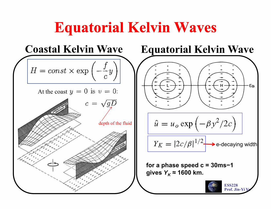
Equatorial Kelvin WavesEquatorial Kelvin WavesCoastal Kelvin Wave Equatorial Kelvin Wave

At the coastAt the coast

depth of the fluid

e decaying widthe-decaying width

for a phase speed c = 30ms−1 i Y 1600 k


gives YK ≈ 1600 km.

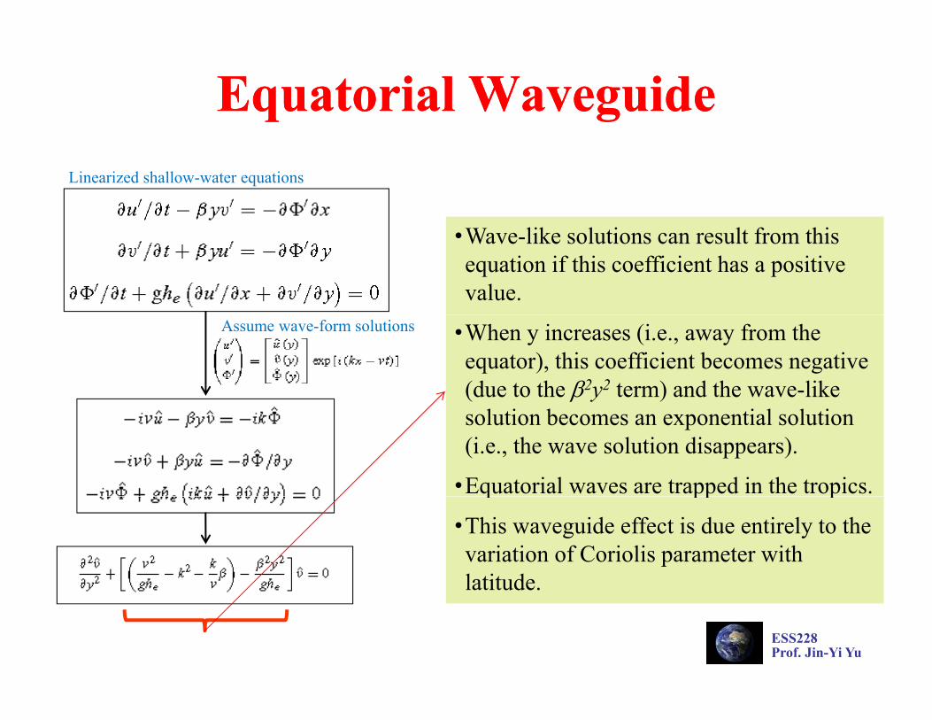
Equatorial WaveguideEquatorial WaveguideLinearized shallow-water equations

•Wave-like solutions can result from this equation if this coefficient has a positive value.

Assume wave-form solutions •When y increases (i.e., away from the equator), this coefficient becomes negative (due to the β2y2 term) and the wave-like solution becomes an exponential solution (i.e., the wave solution disappears).

•Equatorial waves are trapped in the tropics.q pp p

•This waveguide effect is due entirely to the variation of Coriolis parameter with latitude


latitude.

QuaiQuai--Biennial Oscillation (QBO)Biennial Oscillation (QBO)(in Stratosphere)(in Stratosphere)(in Stratosphere)(in Stratosphere)

Quasi-Biennial Oscillation: Easterly and westerly winds alternate every other years


(approximately) in the lower to middle parts of the tropical stratosphere.

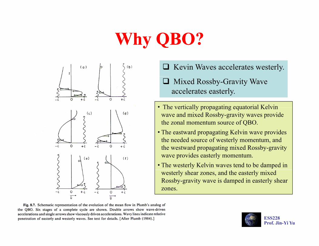
Why QBO?Why QBO?y Qy QKevin Waves accelerates westerly.

Mixed Rossby-Gravity Wave accelerates easterly.

• The vertically propagating equatorial Kelvin• The vertically propagating equatorial Kelvin wave and mixed Rossby-gravity waves provide the zonal momentum source of QBO.

• The eastward propagating Kelvin wave provides th d d f t l t dthe needed source of westerly momentum, and the westward propagating mixed Rossby-gravity wave provides easterly momentum.

• The westerly Kelvin waves tend to be damped in westerly shear zones, and the easterly mixed Rossby-gravity wave is damped in easterly shear zones.


Steady Forced Equatorial MotionsSteady Forced Equatorial MotionsVertically averaged equations for steady motions in the mixed layer:

• The dynamics of steady circulations in a equatorial mixed layer can be approximated by a yset of linear equations analogous to the equatorial wave equations , but with the time derivative terms replaced by linear damping terms.

• In the momentum equations the surface eddy stress is taken to be proportional to the mean velocity in the mixed layer.

I th ti it ti th t b ti i th• In the continuity equation the perturbation in the mixed layer height is proportional to the mass convergence in the layer, with a coefficient that is smaller in the presence of convection than in its

This model can be used to computethe steady surface circulation. p

absence, due to ventilation of the boundary layer by convection.


Gill’s Response to Symmetric HeatingGill’s Response to Symmetric Heating

(from Gill 1980)

• This response consists of a eastward-propagating Kelvin wave to the east of the symmetric heating and a westward-propagating Rossby wave of n=1 to the west.

• The Kelvin wave low-level easterlies to the east of the heating, while the Rossby wave produces low-level westerlies to the west.

• The easterlies are trapped to the equator due to the property of the Kelvin wave.

• The n=1 Rossby wave consists of two cyclones symmetric and straddling the equator


The n 1 Rossby wave consists of two cyclones symmetric and straddling the equator.

• The meridional scale of this response is controlled by the equatorial Rossby radius, which is related to the β-effect and the stability and is typically of the order of 1000km.

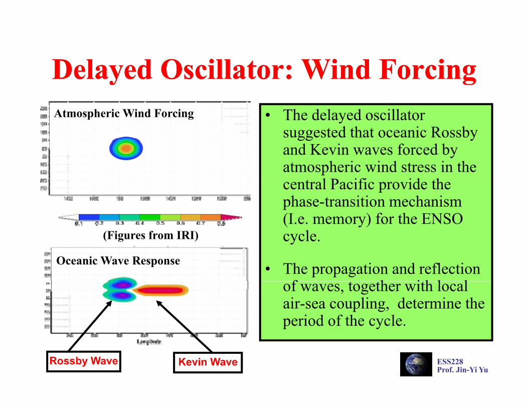
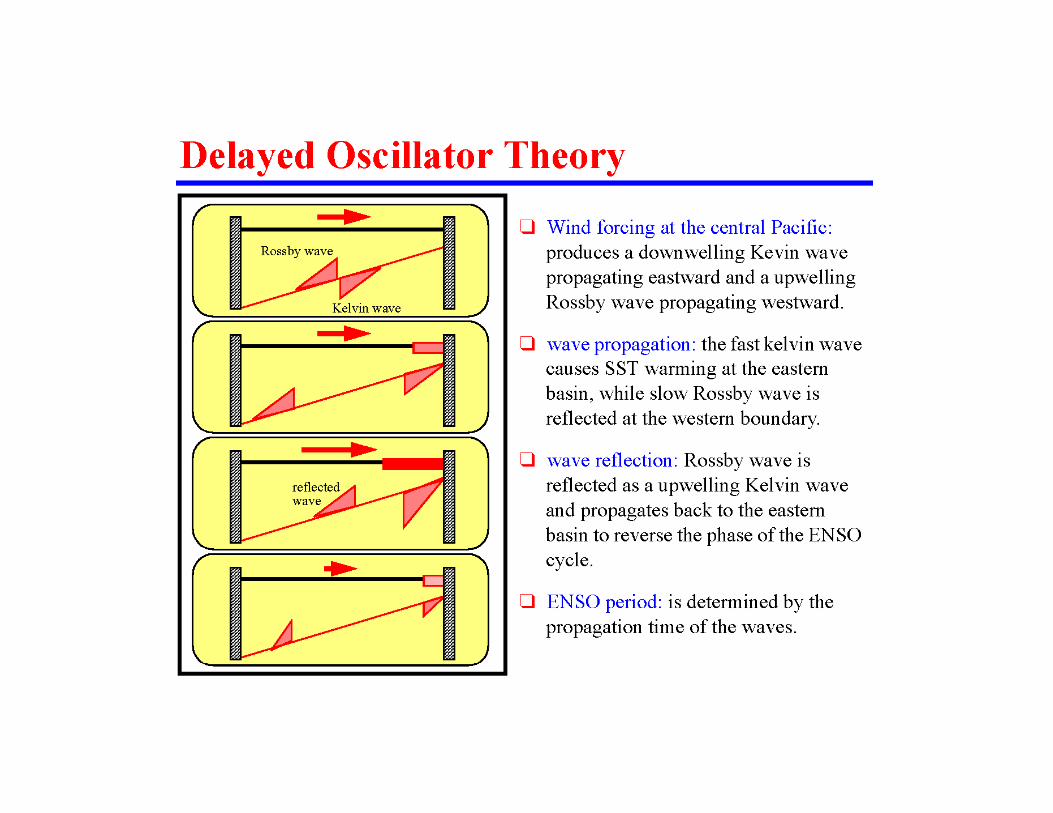
Delayed Oscillator: Wind ForcingDelayed Oscillator: Wind ForcingDelayed Oscillator: Wind ForcingDelayed Oscillator: Wind Forcing• The delayed oscillator

d h i R bAtmospheric Wind Forcing

suggested that oceanic Rossby and Kevin waves forced by atmospheric wind stress in the

l ifi id hcentral Pacific provide the phase-transition mechanism (I.e. memory) for the ENSO cycle.

• The propagation and reflection f h i h l l

Oceanic Wave Response

(Figures from IRI)

of waves, together with local air-sea coupling, determine the period of the cycle.


Rossby Wave Kevin Wave

Wave Propagation and ReflectionWave Propagation and ReflectionIt takes Kevin wave (phase speed = 2.9 m/s) about 70 days to cross the Pacific

equatorial Kelvin wave

days to cross the Pacific basin (17,760km).

It takes Rossby wave about 200 days (phase speed = 0.93 m/s) to cross the Pacific basin.

ESS228Prof. Jin-Yi Yu(Figures from IRI)

coastal Kelvin waves

waves in the atmosphere and oceanswaves ... - …yu/class/ess228/lecture.6.adjustment.all.pdf ·...

Documents