weak gravitational lensing of the cmb -...
TRANSCRIPT

Physics Reports 429 (2006) 1–65www.elsevier.com/locate/physrep
Weak gravitational lensing of the CMB
Antony Lewisa,∗,1,2, Anthony Challinorb
aInstitute of Astronomy, Madingley Road, Cambridge, CB3 0HA, UKbAstrophysics Group, Cavendish Laboratory, J.J. Thomson Avenue, Cambridge CB3 0HE, UK
Accepted 2 March 2006Available online 19 April 2006
editor: M.P. Kamionkowski
Abstract
Weak gravitational lensing has several important effects on the cosmic microwave background (CMB): it changes the CMBpower spectra, induces non-Gaussianities, and generates a B-mode polarization signal that is an important source of confusion forthe signal from primordial gravitational waves. The lensing signal can also be used to help constrain cosmological parameters andlensing mass distributions. We review the origin and calculation of these effects. Topics include: lensing in General Relativity, thelensing potential, lensed temperature and polarization power spectra, implications for constraining inflation, non-Gaussian structure,reconstruction of the lensing potential, delensing, sky curvature corrections, simulations, cosmological parameter estimation, clustermass reconstruction, and moving lenses/dipole lensing.© 2006 Elsevier B.V. All rights reserved.
PACS: 98.80.Es; 98.70.Vc; 98.62.Sb; 8.80.Hw
Keywords: Cosmic microwave background; Gravitational lensing
Contents
1. Introduction . . . . . . . . . . . . . . . . . . . . . . . . . . . . . . . . . . . . . . . . . . . . . . . . . . . . . . . . . . . . . . . . . . . . . . . . . . . . . . . . . . . . . . . . . . . . . . . . . . . . . . . . . . 21.1. The unlensed CMB . . . . . . . . . . . . . . . . . . . . . . . . . . . . . . . . . . . . . . . . . . . . . . . . . . . . . . . . . . . . . . . . . . . . . . . . . . . . . . . . . . . . . . . . . . . . . . . 31.2. CMB lensing order of magnitude . . . . . . . . . . . . . . . . . . . . . . . . . . . . . . . . . . . . . . . . . . . . . . . . . . . . . . . . . . . . . . . . . . . . . . . . . . . . . . . . . . . 41.3. Weak-lensing deflection angle . . . . . . . . . . . . . . . . . . . . . . . . . . . . . . . . . . . . . . . . . . . . . . . . . . . . . . . . . . . . . . . . . . . . . . . . . . . . . . . . . . . . . . 41.4. Photon distribution . . . . . . . . . . . . . . . . . . . . . . . . . . . . . . . . . . . . . . . . . . . . . . . . . . . . . . . . . . . . . . . . . . . . . . . . . . . . . . . . . . . . . . . . . . . . . . . 61.5. Is weak lensing a good approximation? . . . . . . . . . . . . . . . . . . . . . . . . . . . . . . . . . . . . . . . . . . . . . . . . . . . . . . . . . . . . . . . . . . . . . . . . . . . . . . 6
2. Lensing in General Relativity . . . . . . . . . . . . . . . . . . . . . . . . . . . . . . . . . . . . . . . . . . . . . . . . . . . . . . . . . . . . . . . . . . . . . . . . . . . . . . . . . . . . . . . . . . . 72.1. Perturbed photon paths . . . . . . . . . . . . . . . . . . . . . . . . . . . . . . . . . . . . . . . . . . . . . . . . . . . . . . . . . . . . . . . . . . . . . . . . . . . . . . . . . . . . . . . . . . . . 82.2. Geodesic deviation . . . . . . . . . . . . . . . . . . . . . . . . . . . . . . . . . . . . . . . . . . . . . . . . . . . . . . . . . . . . . . . . . . . . . . . . . . . . . . . . . . . . . . . . . . . . . . . 10
2.2.1. Jacobi map in linearly-perturbed cosmology . . . . . . . . . . . . . . . . . . . . . . . . . . . . . . . . . . . . . . . . . . . . . . . . . . . . . . . . . . . . . . . . . . . 122.2.2. Lensing deflection angle . . . . . . . . . . . . . . . . . . . . . . . . . . . . . . . . . . . . . . . . . . . . . . . . . . . . . . . . . . . . . . . . . . . . . . . . . . . . . . . . . . . . 14
2.3. Gauge dependence and observable dipoles . . . . . . . . . . . . . . . . . . . . . . . . . . . . . . . . . . . . . . . . . . . . . . . . . . . . . . . . . . . . . . . . . . . . . . . . . . . 142.3.1. Other gauge effects . . . . . . . . . . . . . . . . . . . . . . . . . . . . . . . . . . . . . . . . . . . . . . . . . . . . . . . . . . . . . . . . . . . . . . . . . . . . . . . . . . . . . . . . 15
∗ Corresponding author.E-mail address: [email protected] (A. Lewis).
1 Latest contact details at http://cosmologist.info2 Formerly at CITA, 60 St. George St, Toronto, Ont., Canada, M5S 3H8.
0370-1573/$ - see front matter © 2006 Elsevier B.V. All rights reserved.doi:10.1016/j.physrep.2006.03.002

2 A. Lewis, A. Challinor / Physics Reports 429 (2006) 1 –65
2.4. Lensing of polarization . . . . . . . . . . . . . . . . . . . . . . . . . . . . . . . . . . . . . . . . . . . . . . . . . . . . . . . . . . . . . . . . . . . . . . . . . . . . . . . . . . . . . . . . . . . 152.5. Higher-order lensing . . . . . . . . . . . . . . . . . . . . . . . . . . . . . . . . . . . . . . . . . . . . . . . . . . . . . . . . . . . . . . . . . . . . . . . . . . . . . . . . . . . . . . . . . . . . . . 162.6. Lensing in other gravity theories . . . . . . . . . . . . . . . . . . . . . . . . . . . . . . . . . . . . . . . . . . . . . . . . . . . . . . . . . . . . . . . . . . . . . . . . . . . . . . . . . . . . 17
3. The lensing potential . . . . . . . . . . . . . . . . . . . . . . . . . . . . . . . . . . . . . . . . . . . . . . . . . . . . . . . . . . . . . . . . . . . . . . . . . . . . . . . . . . . . . . . . . . . . . . . . . . . 173.1. Power spectrum of the lensing potential . . . . . . . . . . . . . . . . . . . . . . . . . . . . . . . . . . . . . . . . . . . . . . . . . . . . . . . . . . . . . . . . . . . . . . . . . . . . . . 183.2. Limber approximation . . . . . . . . . . . . . . . . . . . . . . . . . . . . . . . . . . . . . . . . . . . . . . . . . . . . . . . . . . . . . . . . . . . . . . . . . . . . . . . . . . . . . . . . . . . . 213.3. Non-linear evolution . . . . . . . . . . . . . . . . . . . . . . . . . . . . . . . . . . . . . . . . . . . . . . . . . . . . . . . . . . . . . . . . . . . . . . . . . . . . . . . . . . . . . . . . . . . . . . 21
4. The lensed CMB temperature power spectrum . . . . . . . . . . . . . . . . . . . . . . . . . . . . . . . . . . . . . . . . . . . . . . . . . . . . . . . . . . . . . . . . . . . . . . . . . . . . . 224.1. Simple lowest-order calculation . . . . . . . . . . . . . . . . . . . . . . . . . . . . . . . . . . . . . . . . . . . . . . . . . . . . . . . . . . . . . . . . . . . . . . . . . . . . . . . . . . . . 22
4.1.1. Scale-invariant spectrum . . . . . . . . . . . . . . . . . . . . . . . . . . . . . . . . . . . . . . . . . . . . . . . . . . . . . . . . . . . . . . . . . . . . . . . . . . . . . . . . . . . . 244.1.2. White spectrum . . . . . . . . . . . . . . . . . . . . . . . . . . . . . . . . . . . . . . . . . . . . . . . . . . . . . . . . . . . . . . . . . . . . . . . . . . . . . . . . . . . . . . . . . . . 254.1.3. Small-scale limit . . . . . . . . . . . . . . . . . . . . . . . . . . . . . . . . . . . . . . . . . . . . . . . . . . . . . . . . . . . . . . . . . . . . . . . . . . . . . . . . . . . . . . . . . . 25
4.2. Lensed correlation function . . . . . . . . . . . . . . . . . . . . . . . . . . . . . . . . . . . . . . . . . . . . . . . . . . . . . . . . . . . . . . . . . . . . . . . . . . . . . . . . . . . . . . . . 264.2.1. Exact result . . . . . . . . . . . . . . . . . . . . . . . . . . . . . . . . . . . . . . . . . . . . . . . . . . . . . . . . . . . . . . . . . . . . . . . . . . . . . . . . . . . . . . . . . . . . . . 284.2.2. Conservation of total variance . . . . . . . . . . . . . . . . . . . . . . . . . . . . . . . . . . . . . . . . . . . . . . . . . . . . . . . . . . . . . . . . . . . . . . . . . . . . . . . 294.2.3. Relation between lensed and unlensed correlation functions . . . . . . . . . . . . . . . . . . . . . . . . . . . . . . . . . . . . . . . . . . . . . . . . . . . . . . 29
4.3. Comparison with other CMB temperature secondaries . . . . . . . . . . . . . . . . . . . . . . . . . . . . . . . . . . . . . . . . . . . . . . . . . . . . . . . . . . . . . . . . . 295. Lensing of CMB polarization . . . . . . . . . . . . . . . . . . . . . . . . . . . . . . . . . . . . . . . . . . . . . . . . . . . . . . . . . . . . . . . . . . . . . . . . . . . . . . . . . . . . . . . . . . . 30
5.1. Stokes’ parameters . . . . . . . . . . . . . . . . . . . . . . . . . . . . . . . . . . . . . . . . . . . . . . . . . . . . . . . . . . . . . . . . . . . . . . . . . . . . . . . . . . . . . . . . . . . . . . . 305.2. E and B polarization . . . . . . . . . . . . . . . . . . . . . . . . . . . . . . . . . . . . . . . . . . . . . . . . . . . . . . . . . . . . . . . . . . . . . . . . . . . . . . . . . . . . . . . . . . . . . . 32
5.2.1. Flat-sky harmonics . . . . . . . . . . . . . . . . . . . . . . . . . . . . . . . . . . . . . . . . . . . . . . . . . . . . . . . . . . . . . . . . . . . . . . . . . . . . . . . . . . . . . . . . 335.2.2. Full-sky harmonics . . . . . . . . . . . . . . . . . . . . . . . . . . . . . . . . . . . . . . . . . . . . . . . . . . . . . . . . . . . . . . . . . . . . . . . . . . . . . . . . . . . . . . . . 33
5.3. Lensed polarization power spectra . . . . . . . . . . . . . . . . . . . . . . . . . . . . . . . . . . . . . . . . . . . . . . . . . . . . . . . . . . . . . . . . . . . . . . . . . . . . . . . . . . 345.3.1. Lowest-order calculation . . . . . . . . . . . . . . . . . . . . . . . . . . . . . . . . . . . . . . . . . . . . . . . . . . . . . . . . . . . . . . . . . . . . . . . . . . . . . . . . . . . 345.3.2. Lensed polarization correlation functions . . . . . . . . . . . . . . . . . . . . . . . . . . . . . . . . . . . . . . . . . . . . . . . . . . . . . . . . . . . . . . . . . . . . . . 37
5.4. B-mode confusion: implications for constraining inflation . . . . . . . . . . . . . . . . . . . . . . . . . . . . . . . . . . . . . . . . . . . . . . . . . . . . . . . . . . . . . . 396. Non-Gaussian structure . . . . . . . . . . . . . . . . . . . . . . . . . . . . . . . . . . . . . . . . . . . . . . . . . . . . . . . . . . . . . . . . . . . . . . . . . . . . . . . . . . . . . . . . . . . . . . . . 41
6.1. Three-point function (bispectrum) . . . . . . . . . . . . . . . . . . . . . . . . . . . . . . . . . . . . . . . . . . . . . . . . . . . . . . . . . . . . . . . . . . . . . . . . . . . . . . . . . . 416.2. Four-point function (trispectrum) . . . . . . . . . . . . . . . . . . . . . . . . . . . . . . . . . . . . . . . . . . . . . . . . . . . . . . . . . . . . . . . . . . . . . . . . . . . . . . . . . . . 426.3. Connected n-point correlation functions (cumulants) . . . . . . . . . . . . . . . . . . . . . . . . . . . . . . . . . . . . . . . . . . . . . . . . . . . . . . . . . . . . . . . . . . . 436.4. Polarization . . . . . . . . . . . . . . . . . . . . . . . . . . . . . . . . . . . . . . . . . . . . . . . . . . . . . . . . . . . . . . . . . . . . . . . . . . . . . . . . . . . . . . . . . . . . . . . . . . . . . 436.5. Other non-Gaussian signatures . . . . . . . . . . . . . . . . . . . . . . . . . . . . . . . . . . . . . . . . . . . . . . . . . . . . . . . . . . . . . . . . . . . . . . . . . . . . . . . . . . . . . 446.6. Distinguishing primordial non-Gaussianity . . . . . . . . . . . . . . . . . . . . . . . . . . . . . . . . . . . . . . . . . . . . . . . . . . . . . . . . . . . . . . . . . . . . . . . . . . . 44
7. Reconstructing the lensing potential . . . . . . . . . . . . . . . . . . . . . . . . . . . . . . . . . . . . . . . . . . . . . . . . . . . . . . . . . . . . . . . . . . . . . . . . . . . . . . . . . . . . . . 447.1. Temperature quadratic estimator . . . . . . . . . . . . . . . . . . . . . . . . . . . . . . . . . . . . . . . . . . . . . . . . . . . . . . . . . . . . . . . . . . . . . . . . . . . . . . . . . . . . 457.2. Polarization quadratic estimators . . . . . . . . . . . . . . . . . . . . . . . . . . . . . . . . . . . . . . . . . . . . . . . . . . . . . . . . . . . . . . . . . . . . . . . . . . . . . . . . . . . 467.3. Bayesian methods . . . . . . . . . . . . . . . . . . . . . . . . . . . . . . . . . . . . . . . . . . . . . . . . . . . . . . . . . . . . . . . . . . . . . . . . . . . . . . . . . . . . . . . . . . . . . . . . 47
8. Delensing the lensed sky . . . . . . . . . . . . . . . . . . . . . . . . . . . . . . . . . . . . . . . . . . . . . . . . . . . . . . . . . . . . . . . . . . . . . . . . . . . . . . . . . . . . . . . . . . . . . . . 499. Sky curvature . . . . . . . . . . . . . . . . . . . . . . . . . . . . . . . . . . . . . . . . . . . . . . . . . . . . . . . . . . . . . . . . . . . . . . . . . . . . . . . . . . . . . . . . . . . . . . . . . . . . . . . . . 51
10. Simulations . . . . . . . . . . . . . . . . . . . . . . . . . . . . . . . . . . . . . . . . . . . . . . . . . . . . . . . . . . . . . . . . . . . . . . . . . . . . . . . . . . . . . . . . . . . . . . . . . . . . . . . . . . 5511. Status and applications of CMB lensing . . . . . . . . . . . . . . . . . . . . . . . . . . . . . . . . . . . . . . . . . . . . . . . . . . . . . . . . . . . . . . . . . . . . . . . . . . . . . . . . . . . 55
11.1. Observational status . . . . . . . . . . . . . . . . . . . . . . . . . . . . . . . . . . . . . . . . . . . . . . . . . . . . . . . . . . . . . . . . . . . . . . . . . . . . . . . . . . . . . . . . . . . . . . 5511.2. Cosmological model constraints . . . . . . . . . . . . . . . . . . . . . . . . . . . . . . . . . . . . . . . . . . . . . . . . . . . . . . . . . . . . . . . . . . . . . . . . . . . . . . . . . . . . 5511.3. Cluster and galaxy mass . . . . . . . . . . . . . . . . . . . . . . . . . . . . . . . . . . . . . . . . . . . . . . . . . . . . . . . . . . . . . . . . . . . . . . . . . . . . . . . . . . . . . . . . . . . 56
11.3.1. Cluster lensing of polarization . . . . . . . . . . . . . . . . . . . . . . . . . . . . . . . . . . . . . . . . . . . . . . . . . . . . . . . . . . . . . . . . . . . . . . . . . . . . . . . 5911.4. Moving lenses and dipole lensing . . . . . . . . . . . . . . . . . . . . . . . . . . . . . . . . . . . . . . . . . . . . . . . . . . . . . . . . . . . . . . . . . . . . . . . . . . . . . . . . . . . 60
12. Summary and outlook . . . . . . . . . . . . . . . . . . . . . . . . . . . . . . . . . . . . . . . . . . . . . . . . . . . . . . . . . . . . . . . . . . . . . . . . . . . . . . . . . . . . . . . . . . . . . . . . . . 61Acknowledgements . . . . . . . . . . . . . . . . . . . . . . . . . . . . . . . . . . . . . . . . . . . . . . . . . . . . . . . . . . . . . . . . . . . . . . . . . . . . . . . . . . . . . . . . . . . . . . . . . . . . . . . . 62References . . . . . . . . . . . . . . . . . . . . . . . . . . . . . . . . . . . . . . . . . . . . . . . . . . . . . . . . . . . . . . . . . . . . . . . . . . . . . . . . . . . . . . . . . . . . . . . . . . . . . . . . . . . . . . . 62
1. Introduction
Observations of the cosmic microwave background (CMB) temperature and polarization are a powerful probe of theearly universe and cosmological models. There are now convincing measurements from space, ground and balloons,and many future observations are planned at ever greater resolution and/or sensitivity.3 The basic theory of the CMB iswell understood, with a robust prediction for acoustic oscillations in the primordial plasma giving rise to a characteristic
3 http://lambda.gsfc.nasa.gov/product/

A. Lewis, A. Challinor / Physics Reports 429 (2006) 1 –65 3
pattern of peaks in the anisotropy power spectra (for reviews see e.g. Refs. [1–8]).As ever better data becomes available,observations can resolve smaller effects including various non-linear signals that are important on small scales. One ofthe most important of these is weak lensing: the deflection of CMB photons coming from the last scattering surface bypotential gradients along our line of sight [9–13]. The lensing has a quantitatively important effect on the temperaturepower spectrum, as well as introducing qualitatively new non-Gaussian and polarization signals. The lensing signalhas the same frequency spectrum as the unlensed CMB, and hence cannot easily be distinguished. Understanding andmodelling lensing will therefore be essential for the correct interpretation of near-future CMB data.
This review is aimed at readers familiar with the basic theory of the unlensed CMB; however we shall start with avery brief overview of the relevant properties. We then describe why the effect of lensing is important, give order ofmagnitude estimates, and present a heuristic physical derivation of the deflection angle. We shall use the weak lensingapproximation, so we discuss what this means and whether it is a valid approximation. We give a rigorous derivation ofthe deflection using general relativity (GR) and discuss technical issues in Section 2. In Section 3 we describe how themain effects of lensing can be encapsulated into a single lensing potential, how this affects the CMB, and how to relateit to the matter power spectrum. In Section 4 we derive the important several-percent effect on the CMB temperaturepower spectrum due to lensing, and in Section 5 extend this to the polarization. We explain the importance of the‘B-mode’ polarization signal from lensing, in particular how it is a source of confusion with any primordial signal fromgravitational waves. In addition to the B-mode signal, lensing also introduces a characteristic non-Gaussian signal inthe CMB, as discussed in Section 6.
The extra information in the non-Gaussian structure of the lensed CMB sky actually provides enough informationto learn something about the distribution of the matter causing the lensing. In Section 7 we discuss how the lensingpotential can be reconstructed from observations of the lensed sky alone. If we know something about the lensingpotential, this in principle allows us to ‘delens’ the sky to recover what the CMB would have looked like withoutlensing. We discuss methods for doing this in Section 8, and in particular how the B-mode lensing signal can besubtracted to get at any residual interesting B-mode signal from primordial gravitational waves.
For most of this review we shall use the flat-sky approximation, as it greatly simplifies many of the derivations. InSection 9 we describe the small but potentially important corrections due to the fact that in reality observation directionshave spherical geometry about our observation point. In Section 10 we describe the simulation of lensed CMB skies,essential for testing pipelines and assessing the importance of non-linear physics and other real-world complications.Finally in Section 11 we describe the current observational status and various possible applications of CMB lensing.These include using lensing to constrain dark energy, neutrino mass and other cosmological parameters, as well aslearning about the properties of lensing clusters and galaxies. We also discuss the equivalent effects of moving lensesand dipole lensing.
1.1. The unlensed CMB
Observations show that the CMB temperature is approximately uniform at a temperature of 2.725 K, with anisotropiesat the O(10−5) level [14]. The statistics of the observed CMB anisotropies can be explained as arising from acousticoscillations in the primordial photon-baryon fluid, where the initial perturbations had a Gaussian, purely adiabatic,nearly scale-invariant spectrum [15]. The small size of the perturbations means that linear perturbation theory is veryaccurate, and the acoustic oscillations can be modelled accurately to give robust predictions. What we observe is theepoch at which the universe became neutral at a redshift z ∼ 103, after which CMB photons can propagate more or lessfreely towards us. The perturbations on this high-redshift last-scattering surface are the main contribution to the CMBanisotropy observed, with additional large-scale anisotropies from the integrated Sachs–Wolfe [16] (ISW) effect fromevolving potentials along the line of sight. The process of recombination is not instantaneous as it takes a while formost of the protons and electrons to combine into neutral hydrogen, though viewed today it is extremely thin comparedto the distance to the last scattering surface. It is however slow enough for a photon quadrupole to develop, which thengives rise to polarization through Thomson scattering [17–19]. Thus the last scattering surface is expected to have aninteresting polarization signal as well as an anisotropy in the CMB temperature.
The late-time evolution of potentials gives an additional large-scale temperature anisotropy through the (late-)ISWeffect, which means that the large scale CMB temperature is to some extent correlated with the large scale structurehaving the evolving potentials. Another important late time effect is that of reionization: the epoch at which energeticphotons from stars and quasars can reionize the neutral hydrogen gas. This is thought to have happened at redshifts

4 A. Lewis, A. Challinor / Physics Reports 429 (2006) 1 –65
somewhere between 6z20. The effect is important because the free electrons after reionization scatter some of theCMB photons, damping the small scale anisotropies. Furthermore the CMB quadrupole from last scattering will scatterfrom the free electrons giving rise to a polarization signal that can dominate the expected signal from the last scatteringsurface on large scales. Angular scales smaller than a couple of degrees are however only damped by the reionization:the small-scale CMB signal of most concern for CMB lensing is just proportional to the signal coming from the lastscattering surface. The proportionality constant e−2 depends on the optical depth to the last scattering surface.
There are important second-order signals other than lensing, for example the Sunyaev–Zel’dovich (SZ) effect [20](for reviews see e.g. Refs. [2,21]). These are generally generated at low redshift, and are almost unaffected by lensing[22]. We shall therefore concentrate on the process of lensing of the linear CMB signal from the last scatteringsurface. Since the width of the last scattering surface is small (∼ 100 Mpc comoving) compared to its distance from us(∼ 14 000 Mpc comoving), it is a good approximation to consider it as a single lens source plane. The effect of lensingon the reionization and ISW signals is generally very small as they are only important on large scales.
1.2. CMB lensing order of magnitude
Gravitational lensing of light by matter is expected even in Newtonian physics. If a particle passes a point massat a safe distance, a simple Newtonian argument gives a deflection by an angle 2(R)/c2 (assuming the deflectionis small), where (R) is the potential at the point of closest approach on the undeflected path. As discussed below,a relativistic argument using General Relativity in fact gives twice this result. For weak lensing of the CMB we areinterested in the deflection of a photon’s direction as it travels from the last scattering surface to our observation point.On its way the photon will encounter various under- and over-densities, where in matter domination the potentialsdue to these perturbations are constant in the linear regime. The depth of the potentials is ∼ 2 × 10⁻⁵, so we mightexpect each potential encountered to give a deflection ∼ 10−4. The characteristic size of potential wells given bythe scale of the peak of the matter power spectrum is ∼ 300 Mpc (comoving), and the distance to last scattering isabout 14 000 Mpc, so the number passed through is ∼ 50. If the potentials are uncorrelated this would give an r.m.s.total deflection ∼ 501/2 ×10−4∼ 7×10⁻⁴, corresponding to about ∼ 2 arcmin. We might therefore expect the lensingto become an order unity effect on the CMB at l3000. In fact the unlensed CMB has very little power on thesescales due to damping, so lensing can dominate the observed power at l3000 in the absence of any other secondaries.Of course we have neglected several important effects here, including the correlation of the lensing clumps and thecorrect conversion factors between deflection angles and observed angles; however these order-of-magnitude resultsare about right.
The deflection angles will be correlated over the sky by an angle given by the angular size of a characteristic potential,which is ∼ 300/7000 ∼ 2 for a potential mid-way to last scattering. So although the deflection angles are much smallerthan the size of the degree-scale primary CMB acoustic peaks, they are correlated over a comparable scale. This meansthat the lensing can also have an important effect on the scale of the primary acoustic peaks. If a degree sized hotspot at last scattering is lensed, we expect the spot to appear larger or smaller by ∼ 2′, corresponding to a fractionalchange in size of ∼ 2/60 ∼ 3%. The lensing would not make a spot larger or smaller on average, but it will changethe statistics of the size distribution. The distribution will be 3% wider, corresponding to a ∼ 3% broadening on theacoustic peak: after lensing the size of the spot is less well defined on average. We therefore expect lensing to havepercent level effects on the CMB spectrum on the scale of the primary acoustic peaks, and to dominate the spectrum onarcminute scales.
1.3. Weak-lensing deflection angle
The idea that gravity can bend light dates back over two hundred years [23]. In this subsection we give some simplenon-rigorous derivations to get the correct lowest order result for the deflection angle. In Section 2 we use GR to givea more rigorous derivation and discuss higher-order corrections.
Consider weak lensing of a photon with velocity v by a point of mass M within Newtonian theory. By weak lensingwe mean that deflections due to the lensing are a small perturbations, so deflection angles, etc. are small and may betreated accurately using first-order results. The acceleration due to the mass is given by the gradient of the potential, causing a small transverse acceleration v⊥ = −∇⊥ = GM cos /r2, where is the angle of the photon from themass relative to its angle at distance of closest approach R0. Integrating over the photon path for constant speed |v| = c

A. Lewis, A. Challinor / Physics Reports 429 (2006) 1 –65 5
ψ
*
Fig. 1. Weak lensing geometry for a source (the CMB) at comoving distance ∗ lensed by a potential at distance , assuming a flat universe. Thelensing deflection by an angle changes the observed angle of the source by an angle .
gives a total deflection angle v⊥/|v| = 2GM/c2R0, which is the standard Newtonian result. From now on we shall usenatural units with c = 1.
What changes in GR? The idea that acceleration is due to a force holds in GR, with Dv = −∇⊥ in the Newtoniangauge, where D represents the covariant derivative along the photon world line. However to relate this local accelerationto a change in observed coordinate we also have to account for the curvature of space. The total effect is a local deflectionangle = −2∇⊥, where is a small distance along the photon path. Essentially the GR result is the inertialNewtonian result plus an equal term from the effect of spacetime curvature.
Since potentials are generally small (||10−3; smaller on linear scales) the deflection angles are small, consistentwith our small angle assumption. Now let’s consider how this deflection affects the observed angle of an object atcomoving distance ∗. Comoving distances are related to angles via the angular diameter distance fK(), where
fK() =
K−1/2 sin(K1/2) for K > 0, closed,
for K = 0, flat,|K|−1/2 sinh(|K|1/2) for K < 0, open.
(1.1)
The comoving distance that the source appears to have moved due to the lensing is, in the small angle approximation,fK(∗ − ) = fK(∗) (see Fig. 1). Solving for , the deflection due to the source at is
= fK(∗ − )
fK(∗)= −fK(∗ − )
fK(∗)2∇⊥ (1.2)

6 A. Lewis, A. Challinor / Physics Reports 429 (2006) 1 –65
in the direction of ∇⊥. Adding up the deflections from all the potential gradients between us and the source, we havea total deflection
= −2∫ ∗
0d
fK(∗ − )
fK(∗)∇⊥(n; 0 − ). (1.3)
This is the main result that tells us the deflection angle in terms of the potential gradients along the line of sight. Thequantity 0 − is the conformal time at which the photon was at position n. It is only valid for weak lensing (smallangles), and is only valid to lowest order in the potential. For a flat universe fK(∗ − )/fK(∗) = 1 − /∗.
The lensed CMB temperature in a direction n is given by the unlensed temperature in a deflected direction n′,T (n) = T (n′) = T (n + ). The derivative of the deflection angle defines a magnification matrix (see e.g. Ref. [24])
Aij ≡ ij +
i
j =(
1 − − 1 −2 + −2 − 1 − + 1
). (1.4)
An infinitesimal source with surface brightness I (n +) at position about n before lensing, becomes, after lensing,I (n′ + A). At lowest order the magnification of the intensity ≡ |A|−1 = 1/[(1 − )2 + 2 − ||2] ≈ 1 + 2 isdetermined by the convergence, = − 1
2∇ · . The shear 1 + i2 determines the area-preserving distortion, and theantisymmetric piece determines the rotation. Since Eq. (1.3) is purely a derivative, the antisymmetric rotation vanishes at lowest order.
Shear is the most important effect for galaxy lensing [24] as it makes the galaxy ellipticities correlated in a directiondetermined by the local shear. It can be used without knowing anything about the distribution of the source galaxies.However for the CMB we actually know a lot about the statistical distribution of the unlensed CMB, so shearing is notthe only relevant effect: we can also learn information from perturbation-scale (i.e. non-infinitesimal) magnifications.Including shear and convergence effects on finite scales is most easily described as the remapping of points by thedeflection angle. For this reason we shall usually discuss the deflection angle directly, though the shearing effect on theCMB is real and may be observable through changes to the hot and cold spot ellipticity distribution [25,26].
1.4. Photon distribution
The observed angle of a particular photon from the last scattering surface will be altered due to lensing by potentialgradients along the line of sight. In general there will also be a perturbation to the frequency due to time-varyingpotentials. For linear perturbations this is just the integrated Sachs–Wolfe effect, in general it is the Rees–Sciama effect.By discussing only lensing we are explicitly not considering these frequency shifts, so they must be accounted forseparately along with other secondary signals like SZ.
Lensing by transverse gradients does not change the frequency of the photons, and hence does not change thefrequency distribution in a given direction except via the change in the angle of the source. Hence the lensed CMB hasthe same blackbody spectrum as the unlensed CMB, and multi-frequency observations cannot be used to separate thelensing signal.
The number of photons arriving from a particular sized patch of the last scattering surface will be altered due tolensing: a magnifying lens along the line of sight will cause more photons to reach us from the patch than withoutlensing. However the angular size subtended by the patch is also increased proportionately, so the number of photonsper unit solid angle remains the same. This is the rule that lensing conserves surface brightness. Since the frequencyis also not altered by lensing, it means that lensing of an isotropic last scattering surface is completely unobservable:photons are simply moved around but arrive in the same distribution as before. It is only the presence of anisotropieson the last scattering surface that make the lensing effect interesting.
1.5. Is weak lensing a good approximation?
There are several different aspects of the weak lensing approximation, and ‘weak’ may be used to mean slightlydifferent things in different contexts. The main criterion here is that deflection angles should be small, which is indeedthe case with typical deflections being of the order of arcminutes. Deflections from non-linear structure are also small,with clusters typically giving angles of the order of an arcminute or less, and smaller structures such as galaxies giving

A. Lewis, A. Challinor / Physics Reports 429 (2006) 1 –65 7
only arcsecond deflections. Only a minuscule fraction of lines of sight will come close to black holes or other densebodies that violate the small-angle assumption.
Small deflections are essential for the validity of the Born approximation: calculating the lensing effect usingthe potential gradients along the undeflected path. If deflection angles were large compared to the scale of lensingperturbations this would not be a good approximation and we would have to tackle the much harder problem of ray-tracing along the full deflected photon path. As it is, the Born approximation is excellent for lensing on scales largerthan a few arcminutes (see e.g. Refs. [27,28]). Lensing from a single cluster is also accurately modelled: the deflectionoccurs only in a very thin section of the photon path over which the deflected and undeflected paths are the same.Lensing from multiple clusters is more complicated (see Section 2.5), but rare and irrelevant for a CMB calculation onlarger scales. On very small scales numerical simulations can account for the important additional effects (Section 10).
Another use of the term weak lensing is to exclude cases of ‘strong’ lensing where lines of sight cross, giving caustics,multiple images and points of infinite magnification and shear. This can happen even for tiny deflection angles if thesource is small. For example massive clusters will have a CMB Einstein ring at a radius of ∼ 1 arcmin from the centre,corresponding to the radius at which deflected rays meet at a point on the last scattering surface. Most of our analysiswill in fact apply equally well to ‘strong’ lensing cases, all that we shall require is that deflection angles are small.
Strong lensing and significant magnifications are in fact very common: a large fraction of lines of sight will haveintersected other lines of sight by last scattering [29,30], and many ray bundles will have experienced significant(several percent) magnification due to encounters with small scale structures along the line of sight. Much of thiseffect comes from encounters with very small sub-cluster scale structures, and implies that the light cone has a verycomplex structure on sub-arcminute scales. For the CMB this is fortunately not a problem. On arcminute scales theCMB is very smooth due to diffusion damping. Magnification of a smooth surface does not change what you see atall: if there is a galactic-scale area of large magnification of the CMB this will be essentially unobservable. To have aninteresting effect we need arcminute-scale coherent magnification, corresponding to arcminute scale deflection angles.This is much larger than the amount of deflection produced by most of the structures giving rise to large magnifications.We can therefore proceed to calculate the effect on the CMB down to arcminute scales without worrying at all aboutsmall-scale lenses.4 What matters most for the CMB is the lensing effect of large-scale nearly-linear structures.
Another possible worry is whether non-linear clumping in the late universe violates calculations based on angulardiameter distances and a low-order expansion about a homogeneous Friedmann–Robertson–Walker (FRW) universe.For example if two lines of sight happen to travel exclusively through voids, they will have diverged relative to thepropagation expected in a flat FRW universe [32]. However it turns out that on average the effect on angular diameterdistances is cancelled by convergence caused by propagation through denser regions [29,33–35]. Whether the varianceis important has historically been the matter of much debate (see e.g. Refs. [10,36,12]). As discussed above the totalmagnification variance may be large, but this variation comes largely from very small structures and is largely irrelevantfor the CMB:5 only a convergence field correlated on scales of many arcminutes can affect CMB acoustic scales. Alsonote that potentials are everywhere small, (10−3 even including non-linear features), so we might expect that asystematic analysis based on linear theory that we present in later sections should be accurate to within fairly smallnon-linear corrections [12] (see also Refs. [38,29,30,39]).
We discuss higher-order corrections to the first-order lensing result in more detail in Section 2.5.
2. Lensing in General Relativity
To give a rigorous analysis of the lensing effect we must consider directly the propagation of light rays through theperturbed metric of spacetime. We do this in linearized form using a standard metric-based approach in Section 2.1.An alternative treatment based on the dynamics of infinitesimally-separated rays is given in Section 2.2, which allowsus to define the lensing deflection entirely in terms of directly observable quantities (in linear theory). We employ andassume familiarity with standard GR with the (+ − −−) signature and units such that c = 1.
This section on GR is mathematically more sophisticated than the rest of the review, and tackles some interestingconceptual and technical issues. However readers who are happy with Eq. (1.3) can skip this section and proceed
4 The contrary claim in Ref. [31] is erroneous.5 Ref. [37] claims a several-percent effect on the main CMB acoustic peaks; this is incorrect because the scale dependence and correlation of
the magnification were not properly accounted for.

8 A. Lewis, A. Challinor / Physics Reports 429 (2006) 1 –65
directly to Section 3 as the material in this section is not required for the remainder of the review. For more generalreviews of gravitational lensing see Refs. [24,40–42].
2.1. Perturbed photon paths
We aim to compute the perturbed paths of light rays (null geodesics) in the real clumpy universe. In general, solvingfor the null geodesics requires numerical ray-tracing methods through large simulation volumes [43]. However, forCMB lensing on scales 1 arcmin only weak lensing is expected to be important (see Section 1.5) in which case theperturbations of rays are small and a linearized treatment is appropriate.
We only consider lensing by density perturbations (for lensing by gravitational waves, see Refs. [44,45]), and forconvenience we work in the conformal Newtonian gauge (for a discussion of gauge issues see Section 2.3). The lineelement is then
ds2 = a2()[(1 + 2N) d2 − (1 + 2N)ij dxi dxj ], (2.1)
where is conformal time and the unperturbed spatial metric ij is such that
ij dxi dxj = d2 + f 2K()(d2 + sin2 d2). (2.2)
We shall work to first order in the scalar potentials N and N, so equalities below should be taken to apply at firstorder only. Since for lensing we are only calculating the path of null geodesics with ds2 =0, we can equally well dividethrough by a2()(1 + 2N) and use the simpler conformally-related metric
ds2 = (1 + 4) d2 − ij dxi dxj . (2.3)
Here we defined the ‘Weyl potential’ ≡ (N −N)/2, so called because the general linear scalar-mode Weyl tensorcan be expressed in terms of derivatives of only. The conformal invariance of null geodesics means that they canonly depend on the conformally-invariant Weyl part of the Riemann tensor.
Affinely-parameterized null geodesics are solutions of the geodesic equation,
d2x
d2+
dx
d
dx
d= 0, (2.4)
with g (dx /d)(dx/d) = 0 and ds2 = 0. Note that we have denoted the affine parameter in the conformal metricwith an overhat since it necessarily differs from that in the original frame. In an unperturbed model, there are incomingradial solutions (with a focus at the origin at conformal time 0) with = 0 − .
The 0-component of the geodesic equation gives
d2
d2+ 2
(d
d
)2 d
d+ 2
d
d
dxi
d
xi= 0, (2.5)
where the derivative d/d = + (dxi/d)i is along the (perturbed) ray. Eq. (2.5) is the only equation in
this section that does not also apply in the original metric of Eq. (2.1) since we cannot simply replace by . WithEq. (2.5), we can eliminate the affine parameter from (2.4) in favour of , giving
d2xi
d2 − 2dxi
d
(d
d+ dxj
d
xj
)+ 2ij
xj+ (3)
i
jk
dxj
d
dxk
d= 0, (2.6)
where (3)i
jk are the connection coefficients of the unperturbed three geometry ij . It is very convenient to consider anobserver located at the origin of the spatial coordinates, in which case we are interested in rays that focus at xi = 0.For such rays, d/d = −1 + O() and d/d = O() with an equivalent result for . Making use of these resultsin Eq. (2.6), and evaluating the background connection coefficients, we find
d2
d2 + 2d
d= 0, (2.7)

A. Lewis, A. Challinor / Physics Reports 429 (2006) 1 –65 9
d2
d2 − 2d ln fK()
d
d
d+ 2
f 2K()
= 0, (2.8)
d2
d2 − 2d ln fK()
d
d
d+ 2
f 2K()
1
sin2
= 0, (2.9)
which determine the perturbed rays up to first order in .Eq. (2.7) has d/d + 2 as a first integral, and this must equal −1 by the null condition for the perturbed ray.
Integrating again, we find
= 0 − − 2∫
0
d′, (2.10)
where the integral is along the ray. Since we are only working to first-order in , we can evaluate the integral alongthe unperturbed path = const., = const. and = 0 − . (This is the Born approximation.) Integrating to a fixed, Eq. (2.10) implies a radial displacement. Alternatively, integrating to a fixed implies a variation in the conformaltime at emission; this is a time delay if the potential is negative on-average along the ray, i.e. it passes mostly throughoverdense regions. At the last-scattering surface, the r.m.s. radial delay is ∼ 1 Mpc and is coherent over very largeangular scales [46]. Despite the delay being relatively large, the effect on the CMB is only small due to geometricsuppression effects and the large coherence scale. If we think of plane-wave fluctuations, at a given angular scale l−1
the dominant plane waves to contribute to the CMB fluctuations have their wavevector perpendicular to the line ofsight (and have magnitude k ∼ l/fK(∗) where fK(∗) is the comoving angular-diameter distance to last scattering).A radial displacement has no effect on such plane waves since the displacement then lies in the wavefront. The largesteffect of the radial displacement in the CMB power spectra is actually felt through its cross-correlation with thetransverse lensing displacement, but is still well below 10−4 of the primary power for the temperature and polarizationat l ∼ 1000 (where its contribution peaks), and below 10−3 for the cross-power between temperature and polarization[46]. Since these effects are much smaller than those due to the transverse deflections, we shall not consider radial delaysany further.
Eqs. (2.8) and (2.9) can be integrated twice back to a conformal time 0−∗=∗ using the zero-order result =0−since it only appears in the argument of a function multiplying first-order terms. Then, changing integration order, theintegral over
∫f −2
K (0 − ′) d′ can be done using the explicit form in Eq. (1.1). The result is [47]
(0 − ∗) = 0 −∫ ∗
0d
fK(∗ − )
fK(∗)fK()2
(n; 0 − ), (2.11)
(0 − ∗) = 0 −∫ ∗
0d
fK(∗ − )
fK(∗)fK()
2
sin2
(n; 0 − ), (2.12)
where 0 and 0 label the line of sight n. The small angular displacements − 0 and − 0 form the componentsof the displacement vector on the sphere. Noting that = − 0, but = sin2 ( − 0), we find
= −2∫ ∗
0d
fK(∗ − )
fK(∗)fK()∇n(n; 0 − ), (2.13)
where n is the covariant derivative on the sphere. This derivation of the deflection agrees with the heuristic derivationgiven earlier since we can identify the transverse derivative in Eq. (1.3) with [1/fK()]∇n.
This result actually holds for any theory described in differential geometry with a metric conformally equivalent toEq. (2.1). General relativity specifically only enters through the relation between the Weyl potential and the stress-energytensor, as determined by the Einstein equation. The result is the Poisson equation
( + 3K/a2) = 4G( + ), (2.14)
where is the comoving total density perturbation (i.e. evaluated in the rest-frame of the total energy), is theanisotropic stress, and is the three-dimensional Laplacian. In matter (and dark energy) domination where lensingis important the anisotropic stress is small and the Weyl potential is then directly related to the comoving matterperturbations.

10 A. Lewis, A. Challinor / Physics Reports 429 (2006) 1 –65
2.2. Geodesic deviation
An alternative way to describe gravitational lensing concentrates on the gravitational distortion of the invariantcross-section of infinitesimal bundles of light rays [48–51,38,24,23,40]. The geodesic deviation equation can be usedto follow the evolution in the separation of nearby rays. The advantage of this approach is that it deals exclusivelywith physically-observable quantities; the disadvantage is that by not following rays at finite separation it is notstraightforward to characterize the global properties of the light cone. This means that some important properties ofstrong-lensing situations (i.e. where there is multiple covering of the wave front) such as the number of images a sourceforms, are not readily calculable. However, here we are largely interested in weak lensing and in this limit the approachis essentially equivalent to that given above based on the perturbed geodesics.
We shall express the propagation of the cross-section of the bundle of rays from the 1 + 3-covariant viewpoint ofa field of observers with 4-velocity ua . Working in the geometric-optics limit, we consider two null geodesics xa()
and xa() + xa() that lie in the past light cone of some event A (so all generators of the light cone focus at A). Here is an affine parameter, which we assume takes the same value at A for all rays there. In addition, we chose suchthat ua dxa/d varies smoothly across the geodesics at A. For rays with infinitesimal separation, the connecting vectora() ≡ xa() is then also infinitesimal and lies in the null surface. This means that aka =0 where ka =dxa/d is thewavevector. The equation of motion of the connecting vector is Da/D ≡ kb∇b
a =b∇bka where the right-hand side
involves the (covariant) difference of the wavevectors at on the two geodesics. This follows since, in some arbitrarycoordinate chart,
D
D= d
d+
k
= k (x + x) − k (x) + k
= k +
k
= ∇k . (2.15)
We now introduce the projected connecting vector a⊥ that connects the two geodesics in the local rest space of anobserver with velocity ua , i.e. a⊥ua =0. In general, a⊥ will differ from a by a vector proportional to ka (a displacementalong the geodesic):
a⊥ = a − · u
k · uka . (2.16)
This can be written in terms of the screen projection tensor,
Hab ≡ gab − uaub + eaeb = gab + kakb
(k · u)2 − 2u(akb)
k · u, (2.17)
where ka =(k ·u)(ua +ea) with the (unit) direction ea perpendicular to ua , as a⊥=Hab
b. The screen-projection tensorprojects perpendicular to both ua and ea , so it projects into the two-dimensional rest-space of ua that is perpendicularto the spatial direction of the ray. Under a (local) change of velocity ua → ua , the new projected connecting vector isobtained from that with respect to ua by applying the new screen projection tensor: a⊥ → a⊥ = Ha
bb = Ha
bb⊥.
Since a⊥ and a⊥ differ only by a (null) vector parallel to ka , dot productsbetween projected connected vectors forneighbouring rays are independent of the 4-velocity ua and so the shape and size of the cross-section of a ray bundleare observer-independent.
The propagation equation for a⊥ follows from that for a ; we find
Hab
Db⊥D
= Habc⊥∇ck
b, (2.18)
where we have used kb∇bka = 0. The right-hand side involves the fully projected (two-dimensional) tensor
HacHb
d∇ckd . This is symmetric since, in the geometric optics approximation, ka = ∇aS where S is the phaseof the radiation field. The symmetric tensor can be decomposed irreducibly into a trace part and a trace-free part,
HacHb
d∇ (ckd) = Hab − ab, (2.19)

A. Lewis, A. Challinor / Physics Reports 429 (2006) 1 –65 11
where ≡ ∇aka defines the rate of expansion of the beam cross-section, and the trace-free shear ab defines thearea-preserving distortion. These identifications follow from substituting Eq. (2.19) into Eq. (2.18):
Hab
Db⊥D
= ⊥a − abb⊥. (2.20)
The expansion is thus half the fractional rate of change of invariant area of the ray bundle. If we differentiate Eq. (2.18)again and use the Ricci identity, 2∇[a∇b]kc = Rabc
dkd , we obtain the geodesic deviation equation for the projectedconnected vector in 1 + 3-covariant form:
Hac D
D
(Hcb
Db⊥D
)= Ha
cb⊥kdkeRdbce = Hacb⊥kdkeCdbce − 1
2⊥aRbckbkc. (2.21)
In the last equality, we have decomposed the Riemann tensor in the source term into a part that depends on the Weyltensor, Cabcd , and a part that depends on the Ricci tensor, Rab. The former describes the tidal gravitational action ofnearby matter, while the latter is only operative where there is matter (including dark energy) present by the Einsteinfield equations. The ten degrees of freedom in the Weyl tensor can be represented by two projected (perpendicular toua) symmetric trace-free (PSTF) tensors Eab (‘electric’ part) and Hab (‘magnetic’ part):
Eab ≡ ucudCacbd, Hab ≡ 12 εacdCbe
cdue, (2.22)
where εabc ≡ abcdud is the projected alternating tensor. Writing the Weyl term in Eq. (2.21) in terms of the electricand magnetic parts, we find
Hac D
D
(Hcb
Db⊥D
)= −2(k · u)2b⊥[H〈acHb〉dEcd − H(a
cεb)dHcd ] − 1
2⊥aRbckbkc, (2.23)
where εab ≡ εabcec and the angle brackets denote the PSTF part taken in the 2-dimensional space defined by the
projection Hab.It is convenient to express a⊥ in terms of a two-dimensional orthonormal spacelike basis along the ray, Ea
1 and Ea2 ,
where HabE
bI = Ea
I , I = 1, 2. If we transport these vectors according to HabDEbI /D = 0 (i.e. as parallel as the
projection properties allow), Eq. (2.21) can be written as
d2I
d2 = TIJ J , (2.24)
where I ≡ −EaI ⊥a and the (symmetric) optical tidal matrix isTIJ ≡ −Eb
I EcJ kakdRabcd . Given the initial condition
that a⊥ = 0 at the focus A, the solution of Eq. (2.24) can be written as [38]
I () = −(k · u)−1A DIJ ()
dJ
d
∣∣∣∣A
= DIJ ()J , (2.25)
where the Jacobi map satisfies
d2DIJ
d2 = TIKDKJ , (2.26)
with the initial condition DIJ |A = 0 and dDIJ /d|A = −(k · u)AIJ . In Eq. (2.25), we have introduced the (screen)components I of the infinitesimal angular separation of the rays at A; these are equal to −(k · u)−1
A dI /d|A wherethe proportionality constant arises from converting d to a proper-time interval. The optical expansion and shear canbe determined from the Jacobi map (except at caustics where DIJ is not invertible) by
dDIK
dD−1
KJ = IJ + IJ , (2.27)
where we have used Eq. (2.20). We shall see shortly that for weak lensing in a linearly-perturbed Robertson–Walkergeometry we can relate the symmetric trace-free (STF) part of the Jacobi map to the lensing shear, and the trace to theconvergence.

12 A. Lewis, A. Challinor / Physics Reports 429 (2006) 1 –65
We end this subsection by considering the effect of a change of 4-velocity ua on the Jacobi map. If we changeua → ua , then, given the basis Ea
I (appropriate to ua) along the ray, the basis EaI ≡ Ha
bEbI is appropriate to ua since
it satisfies HabDEbI /D=0. Under both changes, the components of a⊥ are invariant but the components of the angular
separation of rays at A transform to I = (k · u/k · u)AI . It follows that the Jacobi map must scale so as to leaveDIJ /(k · u)A independent of ua . This behaviour is seen to be consistent with its differential equation on noting thatTIJ is invariant but the initial condition on dDIJ /d scales with k · u|A. Finally, we note that the components of theoptical expansion and shear are invariant; in 1 + 3-covariant form the shear transforms as ab → ab = Ha
cHbdcd ,
which leaves the square abab invariant.
2.2.1. Jacobi map in linearly-perturbed cosmologyThe symmetry of the background Robertson–Walker model demands that the Jacobi map must be ∝ IJ . The
determinant of the map is the (invariant) area of the ray bundle per unit solid angle at the focus A and so
DIJ () = a()fK()IJ , (2.28)
where a() is the scale factor at affine parameter and is the comoving distance the ray then travels to A. Thetrace-free part of DIJ thus vanishes in the background and so provides a gauge-invariant description of gravitationallensing in perturbed Robertson–Walker cosmologies. For weak lensing, the STF part describes the shear of images andcan be related to ∇〈ab〉, where a is the deflection angle, as we show shortly. The antisymmetric part of DIJ describesrotation of images; it vanishes to linear order in the perturbations by virtue of Eq. (2.26), the initial conditions, and thefact that the optical tidal matrix is symmetric and, at zero-order, proportional to the identity matrix.
The STF part, D〈IJ 〉, of the Jacobi map evolves according to the STF part of Eq. (2.26). To linear order in theperturbations, we find
d2D〈IJ 〉d2 − 1
af K()
d2[af K()]d2 D〈IJ 〉 = af K()T〈IJ 〉, (2.29)
where we have used Eq. (2.28) and the fact that the STF part of the optical tidal matrix,T〈IJ 〉 vanishes in the background(it depends only on the Weyl curvature). For scalar perturbations, the magnetic part of the Weyl tensor vanishes and theelectric part can be written as a gradient term: Eab =−D〈aDb〉, where the derivatives here are projected perpendicularto ua . The Weyl tensor is gauge-invariant and is generated from the sum of the metric perturbations in the conformalNewtonian gauge: = (N − N)/2. Expressing the Weyl tensor in terms of , we find
T〈IJ 〉 = 2(k · u)2Ea 〈IEbJ 〉Eab = −2
(k · u
af K()
)2
∇〈I∇J 〉, (2.30)
where ∇〈I∇J 〉 involves the components of the (spherical) covariant derivatives of the projection of at along the line
of sight onto the celestial sphere. It is convenient to define IJ ≡ D〈IJ 〉/[af K()] (or, more generally, D〈IJ 〉/√
det D,which is independent of ua). Taking the derivative, and using the linearized form of Eq. (2.27), we can relate IJ to theoptical shear: dIJ /d = IJ . If we substitute for D〈IJ 〉 in Eq. (2.29), we find
d2IJ
d2 − 2d ln fK()
d
dIJ
d= − 2
f 2K()
∇〈I∇J 〉, (2.31)
where we have switched to conformal time using ad = dxaua = (k · u)d and used the zero-order result = A − .It follows that near to the focus, D〈IJ 〉 ∼ O(A − )3 [38] and IJ ∼ O(A − )2. With this boundary condition, thesolution of Eq. (2.31) is
IJ (n) = −2∫ ∗
0d
fK(∗ − )
fK(∗)fK()∇〈I∇J 〉(n; A − ), (2.32)
where we have integrated back to ∗. Comparison with Eq. (2.13) shows that IJ = ∇〈IJ 〉.We now turn to the trace of the Jacobi map, which we denote by D ≡ ∑
IDII . This evolves as
d2D
d2 = −1
2DRabk
akb (2.33)
A. Lewis, A. Challinor / Physics Reports 429 (2006) 1 –65 13
to first order. Note that D does not vanish in the background but instead is given by D = 2a()fK(), and the Ricciterm in Eq. (2.33) also has a zero-order part. It is very convenient to remove that zero-order part of the Ricci tensordue to the expansion by working in the Newtonian gauge and performing the same conformal transformation that wemade in Section 2.1: gab → gab = 2gab, where the conformal factor 2 = [a−2(1 − 2N)]. The conformal Riccitensor has non-zero components
R00 = 2DiDi, Rij = 2Kij − 2DiDj, (2.34)
where Di is the three-dimensional covariant derivative constructed from ij and Di = ij Dj .
Under a conformal transformation, ka = ∇aS is invariant so that ka = −2ka and so, with ka = dxa/d, d = 2d.For an observer following a path xa(), the conformal 4-velocity is ua =−1ua and the conformal increment in propertime is d = d. The Jacobi map is a ratio of proper distances to angles so, for the same observer, the trace D = Dwhere is evaluated at the source position.
The conformal trace evolves according to the ‘hatted’ version of Eq. (2.33), where, for an observer at the origin, theRicci source term is
Rabkakb = 2(k · u)2
(K + ∇2⊥ + 2
d ln fK()
d
), (2.35)
and ∇2⊥ =f −2K ()∇I∇I is the (comoving) transverse Laplacian. We define the first order quantity ≡ 1− D/[2fK()]
where is the perturbed radial distance, so that Eq. (2.33) becomes
d2
d2[2fK()] − 2
d2fK()
d2= D(k · u)2
(K + ∇2⊥ + 2
d ln fK()
d
). (2.36)
We now change variables from to . To first order we have d/d = −(k · u) from the null constraint on ka , and the component of the geodesic equation gives
d2fK()
d2= −(k · u)2fK()
(K + 2
d ln fK()
d
). (2.37)
Using these results and substituting D = 2fK()(1 − ), Eq. (2.36) simplifies to
d2
d2 [fK()] = fK()(∇2⊥ − K), (2.38)
which can be rearranged as
d
d
(f 2
K()d
d
)= ∇I∇I. (2.39)
Near the focus at A, D= 2 +O(2) so that =O(). Integrating twice with a switch of order, and using the boundaryconditions at A, we get
(n) =∫ ∗
0d
fK(∗ − )
fK(∗)fK()∇I∇I(n; A − ). (2.40)
Since D = D in the non-conformal frame we can define the convergence in terms of the trace of the Jacobi map atfirst order as
(n) ≡ 1 − D(n)
2fK(∗)S(∗n; ∗), (2.41)
where S(∗n; ∗) ≡ a(∗)[1 +N(∗n; ∗)] measures the perturbed scale factor at the source. Note that the ∗ here infK(∗) must be the perturbed value, including the radial displacement due to the time delay. The convergence measuresonly the effect on the angular area due to transverse gradients rather than including the effect of the perturbed volumeelement at the source or the change in distance relative to the background due to the time delay.

14 A. Lewis, A. Challinor / Physics Reports 429 (2006) 1 –65
This completes our derivation of the shear and convergence from the Jacobi map in linearly-perturbed Robertson–Walker cosmologies. It is straightforward to show that the result is consistent with that implied by the lensing deflectionangle and radial delays derived in the metric approach in Section 2.1. Note that derivations in e.g. Refs. [48,50] appearto have neglected that time delay and 1 + N terms required for a consistent definition of the magnification matrix interms of the Jacobi map to first order.
2.2.2. Lensing deflection angleThe Jacobi map is directly observable and, as we have seen, for weak lensing the STF part can be related to the
derivatives of the lensing deflection angle, where the latter is calculated by ray-tracing in the conformal Newtoniangauge. This raises the question, can we determine directly from the observable IJ for weak lensing, i.e. can we solve
ab = ∇〈ab〉 (2.42)
on the sphere? Any vector field can be written as a gradient and a divergence-free vector: a = ∇a + εab∇b, where
and are scalar functions on the sphere and εab is the alternating tensor on the sphere. Substituting in Eq. (2.42),we have
ab = ∇〈a∇b〉 − εc〈a∇b〉∇c. (2.43)
Taking the divergence and then taking the divergence or curl again, we find
∇a∇bab = 12∇2(∇2 + 2), εac∇c∇bab = 1
2∇2(∇2 + 2). (2.44)
On the full sphere, the (regular) kernel of ∇2(∇2 + 2) is four-fold degenerate and consists of the l = 0 and l = 1spherical harmonics. It follows that the deflection field is determined up to a dipole vector by the observed ab. Forthe undetermined dipole vector, the curl-like part corresponds to a global (rigid) rotation and hence is unobservable.The l = 1 gradient part does not contribute to the lensing shear, but does contribute to the convergence given by = −∇aa/2 = −∇2/2. From Eqs. (2.40) and (2.32) we can see that this is consistent with our definition of interms of the Jacobi map given in Eq. (2.41) for l > 1. Since ∇2 is only degenerate for the monopole, the observedconvergence can be inverted to recover the dipole of the lensing potential that we cannot get from the shear. Note thatthe measured convergence and hence recovered dipole of the lensing potential and deflection angle do depend on thevelocity of the observer, as discussed further below.
2.3. Gauge dependence and observable dipoles
It is important to understand how the observables depend on the velocity of the observer, v. First, consider theunlensed CMB. The main O(v/c) effect is the generation of a significant dipole from the monopole. At next order,O(v/c)O(/), there are additional effects due to the angular aberration of the anisotropies due to the change of frame:there will only be one choice of v for which there is no aberration. A boost from this frame will produce a dipole-likerotation of directions on the sky, giving an effective magnification and demagnification in opposite directions, leadingto the spacing of the acoustic peaks to be different on opposite hemispheres. In additionO((v/c)2) relativistic aberrationof the monopole will give rise to a frequency dependent kinematic quadrupole (and higher moments), though this willnot concern us here (see Refs. [52,53] for more details). The frame in which the dipole vanishes will not in general bethe same as the frame in which there is no aberration due to the presence of a primordial dipole contribution, and hencethe difference is a gauge-invariant observable.
In linear theory, the observed dipole can be expressed in terms of a gauge-invariant source at last scattering, a gauge-invariant ISW contribution, and a local term that depends on the shear. Hence in the frame in which the shear vanishes,the observed dipole will be just the cosmologically interesting gauge-invariant contributions. The shear vanishes in theNewtonian gauge, and hence the Newtonian gauge is the one in which observers see no local kinematic dipole.
Now consider the effect of lensing. A dipole lensing convergence has the same effect at lowest order as angularaberration due to local motion, magnifying and demagnifying in opposite hemispheres. Our calculations of the observedangles of geodesics must include any first-order angular aberration effect. The explicit results we calculated in theconformal Newtonian gauge show that the Jacobi map contains only terms evaluated at the source or integrated alongthe line of sight. This suggests that there can be no local kinematic angular aberration for a Newtonian gauge observer,

A. Lewis, A. Challinor / Physics Reports 429 (2006) 1 –65 15
consistent with the result above that the kinematic dipole vanishes in this frame. Newtonian gauge observers see nolocal kinematic dipole and no angular kinematic aberration.
For theoretical work it is very convenient to work in the frame in which there is no local angular aberration. Thisis the gauge in which the shear vanishes: the Newtonian gauge. This is why we have consistently used the Newtoniangauge, and will continue to do so. In this gauge N determines the perturbation to the 3-curvature and the integratedlocal 3-expansion; N determines the acceleration; their difference determines the first-order gauge-invariant Weyltensor, and their sum depends on the anisotropic stress (see e.g. the appendix of Ref. [54]).
Our actual motion with respect to the CMB will be somewhat non-linear, and the observed dipole and angles needto be corrected to correspond to the Newtonian gauge predictions. The non-linear effects can be taken out easily byboosting to some frame in which the total observed dipole is zero or small [55]. In principle we could then calculatethe Newtonian gauge dipole by determining the local shear of the new local spatial hypersurface and calculating thetransformation required so that it vanishes. In practice we probably cannot do better than boosting to the frame in whichthe total dipole is zero, which will differ from the Newtonian gauge by ∼ O(10−5) assuming the primordial Newtoniangauge dipole has the expected amplitude. We should then be able to measure the Newtonian gauge convergence dipoleto an error of ∼ O(10−5), which should be useful since it is expected to be 10−4–10−3: the convergence dipole shouldbe measurable to an error much less than cosmic variance.
In summary, the lensing effect of the CMB is real and observable. Only the dipole convergence is sensitive to thegauge, and the Newtonian gauge dipole convergence is measurable to good accuracy in practice. Changing framemerely correspond to adding some angular aberration to the Newtonian gauge result.
2.3.1. Other gauge effectsIt is worth commenting on the other potential gauge issues that arise in a calculation of the weak lensing effect on the
CMB. We are interested in that part of the higher-order CMB anisotropy that arises (approximately) from the projectionof fluctuations over a spacelike last-scattering surface. Consider making a consistent second-order calculation of thisprojection. The possible second-order effects are then: (i) the projection of second-order corrections to the sourceterms (e.g. photon energy and momentum density) evaluated over the zero-order last-scattering surface with the zero-order light cone; (ii) the projection of the first-order sources over the first-order perturbed last-scattering surface withthe zero-order light cone; and (iii) the difference in the projection of the first-order sources over the zero-order last-scattering surface when the first-order perturbed light cone is used instead of the zero-order one. The sum of all threeeffects is gauge-invariant but the individual effects are not separately since they depend on how we identify pointsin the perturbed universe with those in the homogeneous background (on which we think of the perturbations assitting). This identification defines a choice of gauge. As an extreme example, consider fixing the gauge so that for ourgiven observation point, the zero-order light cone coincides with the real perturbed one.6 Then effect (iii) vanishes,which is what we would naively think of as the lensing effect on the CMB. The light cone still has an observableperturbed geometry, but in this gauge it arises only from the local metric fluctuations rather than as an integrated effect.Note that the gauge transformation to this observational gauge is non-local so these two viewpoints are consistent. Inthe observational gauge, CMB lensing appears in effect (i) above since, under the gauge transformation, second-ordersource terms—that depend non-locally on the fluctuations along the line of sight—appear from displacing the first-ordersource fields by first-order amounts in the background.
In the generalization of the conformal Newtonian gauge to second-order (or any other locally-defined gauge),the second-order fluctuations are sourced by non-linear physics in the prior evolution and any additional primordialcontribution. Of the three secondary effects identified above, (iii) is expected to dominate though this has not yet beenproved rigorously with a complete second-order calculation. It is this effect that we have computed here and what wecall the lensing effect on the CMB.
2.4. Lensing of polarization
While CMB photons propagate freely from the last scattering surface, their number density in phase space (i.e.the one-particle distribution function) is conserved. In terms of the specific intensity I seen by a field of observerswith velocity ua , the conserved phase space density implies that I/3 remains constant [57], where is the photon
6 This can be achieved by adopting the observational coordinates of Ref. [56] and references therein.

16 A. Lewis, A. Challinor / Physics Reports 429 (2006) 1 –65
frequency. The polarized specific intensity evolves in exactly the same way provided that it is measured on a basis EaI
that evolves along the geodesic as HabDEbI /D = 0 [58]. If we trace a null geodesic back to last scattering in the
perturbed universe, there are several geometric effects that alter the observed polarization from that in the absence oflensing. First, as with the temperature (or total intensity), we are probing fluctuations on the last scattering surface ata different position. The transverse displacement is what is usually referred to as the gravitational lensing effect anddominates over the effect of the radial displacement [46]. Second, the propagation direction of the perturbed geodesicwhen it reaches last scattering differs from that of a photon propagating along an unperturbed, but displaced, line ofsight n + . The difference arises because the propagation direction accumulates only the lensing deflection angles butthe lensing displacement weights the deflections by the ratio of angular diameter distances from lens to source andobserver to source. The difference is of the same order as the deflection angle (∼ few arcmin) but is much smaller thanthe angular scale of the polarization at last scattering which is quadrupolar and so should not be important (thoughdetailed calculations of this effect have not been reported in the literature). Note that the same process affects theDoppler contribution to the temperature anisotropies. The final geometric process to consider is that in propagatingthe polarization basis along the perturbed line of sight n, the resulting vectors at last scattering will be rotated relativeto an unlensed basis transported along n + . Provided we obtain the basis at n + by parallel transporting that atn along the spherical geodesic connecting the two points, the rotation angle will be ∼ 1 arcmin and the effect shouldalso be negligible. In summary, to a good approximation, the lensed polarization along n is the same as the unlensedpolarization that would be observed along n + on bases that are related by parallel transport between the two linesof sight. We describe lensing of CMB polarization in more detail in Section 5.
2.5. Higher-order lensing
The lowest weak-lensing approximation gives the deflection angle to first order in the Weyl potential . The unlensedCMB is assumed to be first order, so the lensed CMB (n) = (n + ) is in a certain sense second order: it is linearperturbations at last scattering lensed by linear perturbations along the line of sight. However (n + ) = (n) +a∇a(n)+· · ·, with equality only to lowest order in (second order in total). It therefore differs from a second-orderperturbative expansion of by higher order terms. As we shall discuss in Section 4, these higher order terms are in factnot negligible. To get an accurate result from a perturbative expansion in one would need to go to at least third orderand probably higher. Of course a fully consistent second-order analysis would also pick up additional physical effects(for example second-order kinetic-SZ and the small effect of second-order corrections to the sources at last scattering).However if these corrections are small (or can be added separately), the present analysis is likely to be much moreaccurate (and certainly very much easier) than evolving the Boltzmann equation to second or higher order.
As we discuss in Section 3.3, late-time non-linear evolution of can be included within the basic linear- frameworkby simply replacing with its non-linear form. However a full analysis to higher order in must go beyond the Bornapproximation, accounting for deviations of the actual photon path from the undeflected path and multiple scattering.
In the first-order approximation, the deflection angles have zero curl and can be described as the gradient of apotential, = ∇. However at next order in this is no longer true, and in general has a curl-component, an effectcalled field rotation. This is represented by the rotation in the magnification matrix, Eq. (1.4). This lens–lens effectappears in the second-order Born approximation from scattering from two sources (hence O(2)). To see this considerapplying the magnification matrix of Eq. (1.4) consecutively for two different sources with = 0 for each sourceindividually. The resultant magnification matrix is given by the product of the two matrices, which is now no longersymmetric in general, and hence the overall effect includes some rotation. In addition to introducing an antisymmetricterm in the magnification matrix, , the curl of the deflection angle also means that the shear now has a curl component(Eq. (2.43)). This is the B-mode shear often used as a diagnostic in galaxy weak lensing surveys because it is expectedto appear only at second order.
The power spectrum and effect of the field rotation have been calculated in Refs. [43,27]. Because it only appearsat second order its power spectrum is fourth order in the potential. It is around 10−3–10−2 times smaller than theconvergence power spectrum, with most effect on small scales. It is therefore likely to be much less important thanuncertainty in the non-linear potential evolution that gives a much larger effect on these scales. In principle the fieldrotation does provide a limit to how well the B-mode lensing signal can be subtracted (see Section 8), but is not likelyto be important at noise levels 0.25 K-arcmin [27]. Field rotation can also arise from lensing by gravitational waves[45,59], though probably at an unobservably small level.

A. Lewis, A. Challinor / Physics Reports 429 (2006) 1 –65 17
More general studies of second-order corrections to the lensing have been performed in Refs. [60,61,28]. For examplethere is a Born-correction accounting for the transverse displacement of the ray from the undeflected path:7 this canbe included at second order in by performing a transverse Taylor expansion of the potential about the undeflectedpath. This and other corrections are generally very small on the scales relevant for the CMB.
2.6. Lensing in other gravity theories
Any metric gravitational theory than can be described by the metric of Eq. (2.1) would have the same predictionsfor the lensing effect in terms of the Weyl potential that we obtained in GR. How the potential relates to the matterfields can of course change if Einstein’s field equation is changed (for an example in the lensing context see Ref. [62]).Other more general theories may give different results. The relativistic version of MOND due to Bekenstein [63] is abi-metric theory, however in this case the photons are still null geodesics, and many of the predictions for lensing arein fact the same as GR [64] (though of course the relation to the matter is different).
3. The lensing potential
In this section we define the lensing potential, an effective integrated potential useful for calculating the effect ofweak lensing on the CMB anisotropies. We then calculate the power spectrum of the lensing potential, and discussnon-linear corrections and small scale approximations. In later sections we shall use the lensing potential extensivelyfor computing lensing deflection angles and their covariance.
We recall from Eq. (1.3) that the deflection angle of a source at conformal distance ∗ is given in terms of the potential by
= −2∫ ∗
0d
fK(∗ − )
fK(∗)∇⊥(n; 0 − ). (3.1)
The quantity 0 − is the conformal time at which the photon was at position n. It is convenient to write ∇⊥ =(∇n)/fK() so that
= −2∫ ∗
0d
fK(∗ − )
fK(∗)fK()∇n(n; 0 − ), (3.2)
where ∇n represents the angular derivative, equivalent to the covariant derivative on the sphere defined by n. This resultwas derived rigorously at lowest order in Eq. (2.13). We then define the lensing potential,
(n) ≡ −2∫ ∗
0d
fK(∗ − )
fK(∗)fK()(n; 0 − ), (3.3)
so that the deflection angle is given by ∇n. From now on we write this simply as ∇. Note that the lensing potentialappears to be formally divergent because of the 1/ term near =0. However this divergence only affects the monopolepotential, which does not contribute to the deflection angle. We may therefore set the monopole term to zero, and theremaining multipoles will be finite, at which point the lensing potential field is well defined.
For the CMB we can approximate recombination as instantaneous so that the CMB is described by a single sourceplane at = ∗. We neglect the very small effect of late-time sources, including reionization, so a single 2D map of thelensing potential on the sphere contains all the required information. For scales on which the potential is Gaussian,the lensing potential will be Gaussian. On smaller scales non-linear evolution can introduce non-Gaussianity even forGaussian primordial fields, however on acoustic scales this is a small correction so we defer discussion of non-linearevolution to a later section.
For a flat universe fK()=, and for simplicity we shall assume flatness from now on. The geometry only enters intothe calculation of the lensing potential (and unlensed CMB) power spectra, and the generalization to a non-flat universe
7 The Born correction usually refers to evaluating the first-order integral expression for the magnification matrix along the perturbed line of sight.If instead the deflection angle were evaluated along the perturbed line of sight, and then the angular derivatives were taken to form the magnificationmatrix, this would automatically include the lens–lens coupling.

18 A. Lewis, A. Challinor / Physics Reports 429 (2006) 1 –65
is straightforward. Once the lensing potential has been computed deflection angles etc. may be derived without furtherreference to the FRW geometry.
The lensed CMB temperature in a direction n, T (n), is given by the unlensed temperature in the deflected direction,T (n) = T (n′) = T (n + ) where is a deflection angle. At lowest order it is a pure gradient, = ∇.
3.1. Power spectrum of the lensing potential
For a Gaussian lensing potential its power spectrum and the cross-correlation with the CMB contain all the informationwe need to describe fully the statistics of the lensed CMB. We shall therefore now derive a result for the lensing potentialangular power spectrum in terms of the power spectrum of the potential.
We expand 3-D fields into harmonic space using the Fourier convention
(x; ) =∫
d3k
(2)3/2 (k; )eik·x, (3.4)
and define the power spectrum for the assumed statistically homogeneous potential by
〈(k; )∗(k′; ′)〉 = 22
k3 P(k; , ′)(k − k′), (3.5)
where denotes conformal time. Using Eq. (3.3) the angular correlation function for the lensing potential is then
〈(n)(n′)〉 = 4∫ ∗
0d∫ ∗
0d′
(∗ −
∗
)(∗ − ′
∗′
)∫d3k
(2)3
22
k3 P(k; , ′)eik·xe−ik·x′. (3.6)
We now use the result
eik·x = 4∑lm
iljl(k)Y ∗lm(n)Ylm(k), (3.7)
where jl(r) is a spherical Bessel function given in terms of standard Bessel functions by jl(r) = (/2r)1/2Jl+1/2(r).The angular integral over k can then be done using the orthogonality of the spherical harmonics and we have
〈(n)(n′)〉 = 16∑
ll′mm′
∫ ∗
0d∫ ∗
0d′
(∗ −
∗
)(∗ − ′
∗′
)
×∫
dk
kjl(k)jl′(k′)P(k; , ′)Ylm(n)Y ∗
l′m′(n′)ll′mm′ . (3.8)
The lensing potential can be expanded in spherical harmonics as
(n) =∑lm
lmYlm(n), (3.9)
and for a statistically isotropic field the angular power spectrum Cl is defined by
〈lm∗l′m′ 〉 = ll′mm′C
l . (3.10)
Taking the spherical harmonic components of Eq. (3.8) we therefore get
Cl = 16
∫dk
k
∫ ∗
0d∫ ∗
0d′ P(k; 0 − , 0 − ′)jl(k)jl(k′)
(∗ −
∗
)(∗ − ′
∗′
). (3.11)
In linear theory we can define a transfer function T(k; ) so that (k; )=T(k; )R(k) whereR(k) is the primordialcomoving curvature perturbation (or other variable for isocurvature modes). We then have
Cl = 16
∫dk
kPR(k)
[∫ ∗
0dT(k; 0 − )jl(k)
(∗ −
∗
)]2
, (3.12)

A. Lewis, A. Challinor / Physics Reports 429 (2006) 1 –65 19
1 10 100 100010-9
10-8
10-7
10-6
l
[l(l
+ 1
)]2 C
l / 2
Fig. 2. The power spectrum of the deflection angle (given in terms of the lensing potential by ∇) for a concordance CDM model. The lineartheory spectrum (solid) is compared with the same model including non-linear corrections (dashed) from HALOFIT [65].
10 100 1000
10-8
10-7
10-6
l10 100 1000
0
0.1
0.2
0.3
0.4
0.5
0.6
0.7
0.8
0.9
1x 10⁻⁶
l
[l(l
+ 1
)]2 C
l
[l(l
+ 1
)]2 C
l
Fig. 3. Cumulative contribution of different redshifts to the power spectrum of the lensing potential for a concordance CDM model. Note we have
used a log scale for Cl
in the left-hand plot, but linear in the right-hand plot.
where the primordial power spectrum is PR(k). Given some primordial power spectrum this can be computed easilynumerically using Boltzmann codes such as CAMB [66].8 Since it is deflection angles that are physically relevant, it
is usual to plot the power spectrum of the deflection angle ∇ given by l(l + 1)Cl , as shown for a typical model in
Fig. 2. Note that for l1 the Bessel functions go to zero at the origin, jl(k) → 0 as → 0, so the l1 powerspectrum is finite and well defined.
The last scattering surface is a long way away, so the lensing potential has contributions out to quite high redshift asshow in Fig. 3. Nearby low redshift potentials only contribute to the large-scale lensing, so the spectrum is only quite
8 http://camb.info

20 A. Lewis, A. Challinor / Physics Reports 429 (2006) 1 –65
10 100 1000
10-8
10-7
10-6all kk < 10-3
10-3 < k < 0.010.01 < k < 0.10.1 < k < 1
l
[l(l
+ 1
)]2 C
l
Fig. 4. Contributions of different wavenumbers k (in Mpc−1) to the power spectrum of the lensing potential for a concordance CDM model.
1 10 100 1000
0.01
0.1
1
l
Cl
/ (
Cl
Cl )
1/2
ΘΘ
Fig. 5. Correlation of the lensing potential with the CMB temperature.
weakly sensitive to late time non-linear evolution. The contributions from different wavenumber ranges are shownin Fig. 4.
The cross-correlation with the temperature can be worked out using an analogous derivation [67], and a typical resultis shown in Fig. 5. On very large scales the correlation is significant because of the ISW contribution to the large-scaletemperature anisotropy caused by time varying potentials along the line of sight. However on smaller scales where theISW contribution is much smaller, and the lensing potential becomes almost totally uncorrelated to the temperature.The deflection power spectrum peaks at l∼60, at which point the correlation is 10%. For most applications, forexample computing the lensed CMB power spectra, this small correlation can be safely neglected [68]. However the

A. Lewis, A. Challinor / Physics Reports 429 (2006) 1 –65 21
significant large-scale correlation does mean that we already know quite a lot about the large-scale lensing potentialfrom observations of the CMB temperature.
Note the lensing potential has physically relevant modes down to l = 1 (see Section 2.3).
3.2. Limber approximation
At high l the power spectrum P(k) varies slowly compared to the spherical Bessel functions in Eq. (3.11), whichpick out the scale k ∼ l/. Using∫
k2 dk jl(k)jl(k′) =
22 ( − ′), (3.13)
we can Limber-approximate Cl as
Cl ≈ 82
l3
∫ ∗
0 dP(l/; 0 − )
(∗ −
∗
)2
. (3.14)
This approximation is rather good, and is used by the numerical code CMBFAST.9 On small scales it is numericallymuch more efficient than Eq. (3.12) due to the reduced dimensionality of the required integral.
The power spectrum of the potential can be related to the power spectrum of the density perturbations using thePoisson equation, Eq. (2.14). For a flat universe in matter or dark energy domination
P(k; ) = 92m()H 4()
4
P(k; )
k4 = 92m()H 4()
82
P(k; )
k, (3.15)
where P(k; ) is the power in the fractional comoving density perturbation, P(k; ) is the conventionally definedmatter power spectrum, H() is the Hubble parameter, and m() is the fraction of the energy density in matter.
3.3. Non-linear evolution
The most important assumption we have made so far is that the lensing potential is linear and Gaussian. On smallscales this will not be quite correct due to non-linear evolution. The main effect is to change the power spectrumon small scales, and can be estimated from numerical simulations. For simple models, fits to numerical simulationlike the HALOFIT code of Ref. [65] can be used to compute an approximate non-linear, equal-time power spectrumgiven an accurate numerical linear power spectrum at some redshift. HALOFIT is expected to be accurate at the fewpercent level for standard CDM models with power-law primordial power spectra. For more general models, forexample with an evolving dark energy component, further simulations are required (see e.g. [69]). Given a methodfor computing the non-linear power spectrum, a good approximation is simply to scale the potential transfer func-tions T(k, ) of Eq. (3.12) so that the power spectrum of the potential has the correct non-linear form at thatredshift:
T(k, ) → T(k, )
√Pnon-linear
(k; )
P(k; ). (3.16)
Since non-linear effects on Cl are only important where the Limber approximation holds, Eq. (3.16) should be very
accurate.The effect of the non-linear evolution on the power spectrum of the lensing potential is shown in Fig. 2. Although
there is very little effect on scales where the power peaks (l∼60), non-linear evolution significantly increases thepower on small scales. For future reference, this changes the lensed temperature power spectrum C
l by 0.2% forl∼2000, but there are percent level changes on smaller scales. The effect on the B-mode polarization power spectrum
9 http://cmbfast.org

22 A. Lewis, A. Challinor / Physics Reports 429 (2006) 1 –65
is more dramatic, giving a > 6% increase in power on all scales. On scales beyond the peak in the unlensed B-modepower (l1000) the extra non-linear power becomes more important, producing an order unity change in the B-modespectrum on small scales. On these scales the assumption of Gaussianity is probably not very good, and the accuracywill also be limited by the precision of the non-linear power spectrum.
4. The lensed CMB temperature power spectrum
Observations of the CMB temperature power spectrum are becoming increasingly accurate. The anisotropies at lastscattering are expected to be closely Gaussian, and the power spectrum, Cl , can be worked out accurately in lineartheory. However we observe the lensed temperature field, which will have a modified power spectrum (as well as havinga non-Gaussian structure). This effect must be taken into account to obtain accurate cosmological parameter constraintsfrom CMB observations.
We first describe a simple derivation of the lensed Cl using a series expansion in the deflection angle, which turnsout to be a good way to understand the most important effects [67]. However it is not very accurate because on smallscales the lensing deflection will be of the same order as the wavelength being deflected, and a perturbative expansionin the deflection angle is then not a good approximation. We therefore also discuss a non-perturbative calculation ofthe lensing effect by considering the correlation function [12,70]. Another approach to the lensed power spectrum isdescribed in Ref. [13].
A calculation of the lensed power spectrum to within cosmic variance must take account of sky curvature, howeverthis effect is small so we postpone discussion of curvature corrections to Section 9. Non-linear evolution must alsobe included to get the small-scale spectrum accurately, and can be included in the Gaussian approximation by using alensing potential computed using the non-linear power spectrum as described in Section 3.3.
4.1. Simple lowest-order calculation
As a first calculation of the effect on the CMB, we compute the lensing power spectrum at lowest order in Cl . To
do this we work in harmonic space, using the symmetric flat-sky 2D Fourier transform convention for the temperaturefield:
(x) =∫
d2l2
(l)eil·x, (l) =∫
d2x2
(x)e−il·x. (4.1)
We shall assume that the temperature fluctuations are statistically isotropic, which means that any statistical averagecannot depend on where on the sky (or in which orientation) it is evaluated. The correlation function of the temperatureat two points can therefore only depend on the separation between the points
〈(x)(x′)〉 = (|x − x′|). (4.2)
With this assumption the covariance of the unlensed Fourier components is
〈(l)∗(l′)〉 =∫
d2x2
∫d2x′
2e−il·xeil′·x′
(|x − x′|)
=∫
d2x2
∫d2r2
ei(l′−l)·xeil′·r(r)
= (l′ − l)∫
d2r eil·r(r). (4.3)
In the second line we changed variables to r = x − x′, and have defined r ≡ |r|. We define the power spectrum Cl
so that
Cl =
∫d2r eil·r(r) =
∫r dr
∫dr eilr cos(l−r)(r) = 2
∫r drJ 0(lr)(r). (4.4)

A. Lewis, A. Challinor / Physics Reports 429 (2006) 1 –65 23
Here we have used the Bessel function Jn(r) that arises from integrating the result
eir cos =∞∑
n=−∞inJn(r)e
in = J0(r) + 2∞∑
n=1
inJn(r) cos(n). (4.5)
The power spectrum for our statistically isotropic temperature field is therefore diagonal in l, and is given by
〈(l)∗(l′)〉 = Cl (l − l′). (4.6)
We can perform a similar Fourier transform for the lensing potential , and define the corresponding power spectrum
Cl for the flat sky (equivalent to Eq. (3.10) on small scales).Lensing re-maps the temperature according to
(x) = (x′) = (x + ∇)
≈ (x) + ∇a(x)∇a(x) + 12∇a(x)∇b(x)∇a∇b(x) + · · · . (4.7)
As discussed, the series expansion is not a good approximation on all scales. However it can be used to get qualitativelycorrect results for the lensed Cl , and is useful for giving a simple derivation to aid understanding. Introducing theFourier transform of the lensing potential, (l), we have
∇(x) = i∫
d2l2
l(l)eil·x, ∇(x) = i∫
d2l2
l(l)eil·x. (4.8)
Taking the Fourier transform of (x) and substituting we get the Fourier components to second order in
(l) ≈ (l) −∫
d2l′
2l′ · (l − l′)(l − l′)(l′)
− 1
2
∫d2l12
∫d2l22
l1 · [l1 + l2 − l]l1 · l2(l1)(l2)∗(l1 + l2 − l). (4.9)
We now work out the power spectrum of the lensed field (x) to lowest order in Cl . We can neglect the 〈(l)(l)〉
correlation since the small scale temperature at last scattering is almost uncorrelated with the late-time potentialsresponsible for the lensing, and the correlation only has a tiny effect on the result. The covariance for the lensedtemperature remains diagonal due to statistical isotropy, so that
〈(l)∗(l′)〉 = (l − l′)Cl . (4.10)
At lowest order in Cl there are contributions from the square of the first order term in , and also a cross-term from
the zeroth and second order terms. Using (l) = ∗(−l), we get
Cl ≈ C
l +∫
d2l′
(2)2 [l′ · (l − l′)]2C|l−l′|C
l′ − C
l
∫d2l′
(2)2 (l · l′)2Cl′ . (4.11)
This simplifies to the final result [67]
Cl ≈ (1 − l2R)C
l +∫
d2l′
(2)2 [l′ · (l − l′)]2C|l−l′|C
l′ . (4.12)
Here we have defined half the total deflection angle power
R ≡ 1
2〈|∇|2〉 = 1
4
∫dl
ll4C
l , (4.13)
where for typical models R ∼ 3 × 10⁻⁷, corresponding to an rms deflection of ∼ 2.7 arcmin. The integral termhas the form of a convolution of the unlensed temperature spectrum with the lensing potential power spectrum.

24 A. Lewis, A. Challinor / Physics Reports 429 (2006) 1 –65
10 100 1000 10000
100
102
104
500 1000 1500 2000 2500 3000-0.1
-0.05
0
0.05
0.1
0.15
0.2
0.25
l
l
∆Cl
/ Cl
ΘΘ
l(l +
1)C
l / 2
K
2Θ
Fig. 6. Top: the lensed temperature power spectrum (solid) and the unlensed spectrum (dotted), compared to the large l asymptotic result of Eq.(4.16) (dashed). Bottom: the fractional change in the power spectrum due to lensing. Both plots are for a typical concordance CDM model.
This convolution serves to smooth out the main peaks in the unlensed spectrum, which is the main qualitative effecton the temperature spectrum on large scales. The effect is shown in Fig. 6, and is several percent at l1000. On smallscales where there is little power in the unlensed CMB the convolution transfers power from large scales to small scalesto increase the small-scale power.
4.1.1. Scale-invariant spectrum
The deflection angle power spectrum l4Cl peaks on large scales l∼50 as shown in Fig. 2. For l?50 the bulk of the
convolution term in Eq. (4.12) therefore comes from scales with l∼l′. Consider what happens if the temperature powerspectrum is scale invariant on relevant scales, l2C
l = const. The lensed power spectrum is then given by
Cl ≈ (1 − l2R)C
l + l2Cl
∫d2l′
(2)2
[l′ · (l − l′)]2
l′2 C
|l−l′|
= (1 − l2R)Cl + l2C
l
∫d2l1(2)2
[(l1 − l) · l1]2
(l − l1)2 Cl1
= (1 − l2R)Cl + l2C
l
∫dl1
l1
l41C
l1
4+ l2C
l
∫ ∞
l
dl1
l1
l41C
l1
4(1 − (l/ l1)
2)
= Cl
⎡⎣1 + l2
∫ ∞
l
dl1
l1
l41C
l1
4(1 − (l/ l1)
2)
⎤⎦ . (4.14)
The remaining integral is generally small, and the lensed spectrum only deviates from scale invariant at the O(10−3)
level. If there were no lensing power at l > l0, scale invariance would be preserved on scales l > l0: a large-scalelensing mode magnifies and demagnifies small-scale structures, which has no effect if the structures are scale invariant.Lensing of the CMB is important because the acoustic oscillations and small scale damping give a well definednon-scale-invariant structure to the power spectrum.

A. Lewis, A. Challinor / Physics Reports 429 (2006) 1 –65 25
4.1.2. White spectrumThough of limited relevance for CMB lensing, it is also interesting to consider the lensing effect on a white spectrum
with Cl = const. In this case we have [71]
Cl ≈ (1 − l2R)C
l + Cl
∫d2l1(2)2 [l1 · (l + l1)]2C
l1
= Cl + C
l
∫dl1
l1
l61C
l
2
= Cl (1 + 4〈2〉), (4.15)
where we used = −∇2/2 to identify the variance of the convergence. Thus a white spectrum lenses to a whitespectrum scaled by a factor depending on the total power in the lensing convergence.
4.1.3. Small-scale limitThe fact that l2R ∼ O(1) at l∼2500 in Eq. (4.12) serves as a reminder that the lowest-order series-expansion result
is not likely to be accurate on all scales. This is because on scales with l∼2000 the deflection angles are becomingcomparable to the wavelength of the unlensed fields, so the Taylor expansion is no longer a good approximation. Foraccurate results at all l we need to perform a calculation that does not rely on a series expansion. In principle thiscould be done by extending the above calculation to all orders [72], however in practice it is most easily done byconsidering the correlation function as we discuss in the next section. See also Ref. [71] for an interesting alternativeapproach.
Although the series expansion is not accurate for l∼2000, on very small scales, l?3000, the series expansionresult is actually accurate again. This is because the perturbations in the unlensed spectrum are nearly wiped out bydiffusion damping, so the unlensed spectrum has very little power and can be described accurately on small scalesby a single gradient term. Although the deflection angles are larger than the unlensed wavelengths on these scales,a large bulk deflection is unobservable so the effect on the observed small scales is the same as if the lensed fieldcould be described by T ≈ ∇ · ∇T . In particular if we set C
l = 0 in the first term of Eq. (4.12) and use l′>l weobtain [73,67]
Cl ≈
∫d2l′
(2)2 [l′ · (l − l′)]2C|l′−l|C
l′
≈ Cl
∫d2l′
(2)2 [l′ · l]2Cl′
≈ l2Cl
∫dl2
l2
l42C
l2
4
≈ l2Cl R. (4.16)
Here we defined
R ≡ 1
2〈|∇T |2〉 = 1
4
∫dl
ll4C
l ∼ 109 K2 (4.17)
similarly to Eq. (4.13) to measure the power in the unlensed CMB temperature gradient. The lensed CMB power is
therefore proportional to the unlensed gradient power R, and to the power in the deflection angle l2Cl .
This can be understood as follows. Small scale clumps (or voids) in the lensing potential disturb the smooth back-ground CMB gradient by the varying deflection angle over the clump, giving a clump-scale feature in the observedtemperature. The amplitude of this wiggle is proportional to both the strength of the background gradient, and the sizeof the deflection angles. The wiggle is on the same scale as the clump, and the lensed power spectrum therefore follows

26 A. Lewis, A. Challinor / Physics Reports 429 (2006) 1 –65
the scale dependence of the deflection angle. See Section 11.3 for further discussion of the lensing effect from smallscale fields, and in particular for the signal from non-linear structures such as clusters.
4.2. Lensed correlation function
For a more accurate calculation of the lensing effect on all scales we now calculate the lensed correlation function inthe flat-sky limit, broadly following the method of Ref. [12]. The correlation function is invariant under displacements:it only depends on the separation of the two points. Unlike the series expansion approach it is therefore insensitive tobulk unobservable shifts of the unlensed CMB. The result only depends on the correlation structure of the differenceof deflection angles, which is what is directly observable.
Lensing re-maps the temperature according to
(x) = (x + ), (4.18)
where now to get an accurate result on all scales we do not expand in = ∇. The lensed correlation function (r) isgiven by
(r) ≡ 〈(x)(x′)〉= 〈(x + )(x′ + ′)〉
=∫
d2l2
∫d2l′
2〈eil·(x+)e−il′·(x′+′)〉〈(l)(l′)∗〉
=∫
d2l
(2)2 Cl eil·r〈eil·(−′)〉. (4.19)
As before we have defined r ≡ x−x′ and neglected the small correlation between the CMB temperature and the lensingpotential. The remaining average is over the deflection angle. For a Gaussian variate y with zero mean and variance2
y ≡ 〈y2〉 we have
〈eiy〉 = 1√2y
∫ ∞
−∞dy eiye−y2/22
y = 1√2y
∫ ∞
−∞dy e−(y−i2
y)2/22y e−2
y/2
= e−〈y2〉/2. (4.20)
Since we are assuming is a Gaussian field, l · ( − ′) is a Gaussian variate, and the expectation value in Eq. (4.19)therefore reduces to
〈eil·(−′)〉 = exp(− 12 〈[l · ( − ′)]2〉). (4.21)
To compute the average in the exponential we need to work out the correlation tensor
〈i′j 〉 = 〈∇i(x)∇j(x′)〉 =
∫d2l
(2)2 li ljCl eil·r. (4.22)
By symmetry, the correlator can only depend on ij and the trace-free tensor r〈i rj〉 ≡ ri rj − 12ij where r = r/r .
We evaluate these parts by taking the trace to give
Cgl(r) ≡ 〈 · ′〉
=∫
d2l2
l2Cl eil·r
= 1
2
∫dl l3C
l J0(lr), (4.23)

A. Lewis, A. Challinor / Physics Reports 429 (2006) 1 –65 27
and contracting with r〈i rj〉 to give
Cgl,2(r) ≡ − 2r〈i rj〉〈i′j 〉
= − 2∫
d2l
(2)2 r〈i rj〉li ljCl eil·r
= − 2∫
d2l
(2)2
l2 cos 2
2C
l eil·r
= 1
2
∫dl l3C
l J2(lr). (4.24)
Here we defined as the angle between l and r, and used Eq. (4.5) to express the integrals in terms of Bessel functions.Using these results we have
〈i′j 〉 = 1
2Cgl(r)ij − Cgl,2(r)r〈i rj〉. (4.25)
We can now compute the required expectation value in Eq. (4.21):
〈[l · ( − ′)]2〉 = li lj 〈(i − ′i )(j − ′
j )〉= l2[Cgl(0) − Cgl(r)] + 2li lj r〈i rj〉Cgl,2(r)
= l2[2(r) + cos 2Cgl,2(r)]. (4.26)
We have defined the quantity 2(r) ≡ Cgl(0)−Cgl(r)= 12 〈(−′)2〉, which is half the variance of the relative deflection
of the two points.Putting this all together we get the final result for the lensed correlation function
(r) =∫
d2l
(2)2 Cl eil·r exp
(−1
2〈[l · ( − ′)]2〉
)
=∫
d2l
(2)2 Cl eilr cos exp
(−1
2l2[2(r) + cos 2Cgl,2(r)]
)
=∫
d2l
(2)2 Cl eilr cos e−l22(r)/2
(1 − l2
2cos 2Cgl,2(r) + · · ·
)
=∫
dl
l
l2Cl
2e−l22(r)/2
[J0(lr) + 1
2l2Cgl,2(r)J2(lr) + · · ·
]. (4.27)
Here for simplicity we expanded in Cgl,2 before integrating over . Since Cgl,2 is significantly less than 2 (as shownin Fig. 7), the perturbative expansion in Cgl,2 converges much faster than one in 2 and this is a good approximation
for the scales of most interest. Note that it is important to keep exp(−l22/2) as the main non-perturbative term in Cl .
The lensed correlation function is related to the lensed Cl by Eq. (4.4). The calculation of the correlation function andthe inversion to the power spectrum is numerically very efficient, requiring only one dimensional sums and integrals.It is used in the numerical codes CMBFAST [74], CMBEASY [75] and CAMB [66]. Results to the next order in Cgl,2are given in [70], along with the generalization to a non-flat sky. This is sufficient for a calculation to within cosmicvariance on scales where the non-linear power spectrum can be computed accurately and non-Gaussian corrections canbe neglected. The full result is implemented in the public CAMB code.
The difference between the result using the accurate correlation-function method and the lowest-order series-expansion result is shown in Fig. 8. The series expansion result is accurate on large scales where the deflection angle ismuch smaller than the wavelength of the modes, and also on very small scales where the unlensed CMB has little powerand can be accurately approximated by a single gradient term. In the intermediate regime the series-expansion result isnot accurate and the non-perturbative correlation function method must be used. Note that the errors are percent levelby l∼2000, amounting to a significant fraction of the lensing effect on these scales.

28 A. Lewis, A. Challinor / Physics Reports 429 (2006) 1 –65
Fig. 7. The functions 2() ≡ Cgl(0) − Cgl() [solid] and Cgl,2() [dashed] as a function of angular separation (in radians) for a typical
concordance model. For accuracy the results are calculated using the full-sky generalization, and use the linear power spectrum for Cl
.
1000 2000 3000 4000 5000 6000 7000
-0.1
-0.05
0
0.05
0.1
∆Cl /
Cl
l
Fig. 8. Fractional difference between the lensed Cl results using the series-expansion method to lowest order in Cl
compared to the more accuratecorrelation function result (temperature (solid) and E-polarization (dashed; see Section 5)).
4.2.1. Exact resultAlthough the series expansion we used in Eq. (4.27) is fully adequate for an accurate flat-sky calculation in most
cases relevant for the CMB, for completeness we note that the integral in Eq. (4.27) can actually also be evaluatedexactly as an infinite sum. Substituting r → ir in Eq. (4.5) and using Jn(ir) = inIn(r) where In is a modified Besselfunction we have
e−r cos =∞∑
n=−∞(−1)nIn(r)e
in = I0(r) + 2∞∑
n=1
(−1)nIn(r) cos(n). (4.28)
Using this and Eq. (4.5) to expand the exponentials in Eq. (4.27), and integrating over , leads to the exact flat-skyweak lensing result for uncorrelated Gaussian fields with the temperature on a single source plane
(r) =∫
dl
l
l2Cl
2e−l22(r)/2
∞∑n=−∞
In[l2Cgl,2(r)/2]J2n(lr). (4.29)
A. Lewis, A. Challinor / Physics Reports 429 (2006) 1 –65 29
Note that for |n| > 0 there are two equal contributions from n=|n| and −|n|. Also note that although In(r) → er/√
2r
for large r, because 2(r)Cgl,2(r) the combination e−l22(r)/2In(l2Cgl,2(r)/2) goes to zero as l → ∞. For a fixed
maximum l, only a low number of terms in |n| near zero are required to achieve good accuracy. This general form maybe useful for calculating the lensing effect on very small scales l?103 when C
l has small scale power and a low orderexpansion in Cgl,2 is insufficient. One non-CMB example where this may be useful is calculating the lensing effect onthe 21-cm power spectrum [71].
4.2.2. Conservation of total varianceThe variance at a point (0) = 〈|(x)|2〉 can be obtained by noting that Cgl,2(0) = 2(0) = 0 and In(0) = n0. It
follows from Eq. (4.29) that the total power is conserved by lensing
(0) = (0) =∫
dl
l
l2Cl
2=∫
dl
l
l2Cl
2= 〈|(x)|2〉 = 〈|(x)|2〉. (4.30)
This reflects the fact that weak lensing only alters photon directions, and hence the spatial correlation structure, butdoes not change the variance in any given direction. We are observing the same photons, just in a slightly differentdirection.
4.2.3. Relation between lensed and unlensed correlation functionsWe can also calculate the lensed correlation function in terms of the unlensed one using Eqs. (4.27) and (4.4):
(r) =∫
d2l
(2)2
∫d2r′ e−il·r′
(r ′)eil·r exp
(−1
2l2[2(r) + cos 2(l − r)Cgl,2(r)]
)
=∫
d2r′(r ′)∫
d2l
(2)2 eil·(r−r′)e−l22(r)/2e−(l2r1−l2r2)Cgl,2(r)/2
=∫
d2r′ (r ′)
2√
4(r) − C2gl,2(r)
exp
(− (r − r′)2
2[2(r) + Cgl,2(r)] − r′2 sin2(r − r′)Cgl,2(r)
[4(r) − C2gl,2(r)]
). (4.31)
In the middle line, we have resolved l into its components lr1 and lr2 parallel and perpendicular to r. In an isotropicapproximation where Cgl,2(r)=0, this is an isotropic Gaussian convolution of the two-dimensional correlation function,with a smoothing width 2(r) that depends on r. This smoothing of features in the correlation function correspondsin harmonic space to the smoothing of the C
l peaks. The angular integral can also be done to express the answer interms of modified Bessel functions, but the result it not especially enlightening or useful.
4.3. Comparison with other CMB temperature secondaries
In addition to weak lensing, there are a variety of other non-linear effects on the CMB. The thermal SZ effect [20,21]due to scattering from hot electrons can be significant on small scales. This signal has a frequency spectrum differentto that of the linear CMB and hence can in principle easily be distinguished. However there are other non-linear effectswhich, like CMB lensing, have the same frequency spectrum as the primordial anisotropies. These are a potential sourceof complication when analysing the lensed CMB as they cannot be easily distinguished, and may indeed be correlatedwith the lensing signal.
The kinetic SZ effect is the main such effect for the temperature anisotropies [76–78], arising from scattering fromelectrons in a bulk flow of a non-linear perturbation with respect to the CMB. It is closely related to the second-orderOstriker–Vishniac effect [79], they are both essentially Doppler terms determined by the electron velocity projectedalong the line of sight direction. These effects combine with additional signals due to patchy reionization [80] togive a significant non-linear anisotropy from around the epoch of reionization and afterwards. Current uncertainties inthe reionization history and morphology make detailed predictions for the spectrum difficult, and at the moment thisuncertainty gives rise to a percent-level uncertainty in the expected total C
l at l = 2000 [76]. Fig. 9 shows a samplecomparison. Precision cosmology from the temperature damping tail will require accurate modelling of both lensingand the kinetic SZ effect, and they may indeed be significantly correlated [77]. For the polarization spectra the kineticSZ effect is much smaller [81,76], and lensing is likely to be the dominant effect.

30 A. Lewis, A. Challinor / Physics Reports 429 (2006) 1 –65
10 100 1000 10000
100
101
102
103
104
tSZ: 145GHz
kSZ+OV
Lensing
l
l(l +
1)C
l / 2
K
2Θ
Fig. 9. Contributions to the total blackbody-spectrum temperature anisotropy Cl
(thick solid) from CMB lensing and kinetic SZ (kSZ) plusOstriker–Vishniac (OV) for a typical CDM model with inhomogeneous reionization. The kSZ + OV signal is taken from a model in Ref. [76],and can vary depending on parameters. The spectrally-distinguishable thermal SZ signal is shown dashed, though this also depends strongly onparameters. On very small scales kSZ + OV dominates both the unlensed (dotted) and lensed CMB power spectrum.
Other non-linear signals include the Rees–Sciama effect, a late time ISW-like anisotropy generated by photonspropagating though potential wells that are evolving because of non-linear growth or their bulk motion [82]. This isgenerally subdominant on all scales [83], and hence is not a major concern. There is also a second-order time-delayeffect due to the varying potentials along the line of sight. However the effect turns out to be much weaker than thelensing contributions, and can probably be neglected [84,46].
5. Lensing of CMB polarization
The presence of a non-zero photon quadrupole at last scattering means that there will be an interesting polarizationsignal. As for the temperature, the observed polarization field will have been lensed by potential gradients along the lineof sight, and we need to model this effect. The polarization orientation along a lensed light beam is simply transportedin the manner described in Section 2.4. At lowest order this means that the orientation of the polarization in the observeddirection n and the lensed direction n′ will be the same with respect to the geodesic connecting the two points. Theeffect of lensing may therefore be modelled in a manner similar to the temperature lensing, with the added complicationthat the polarization is a tensor field that is parallel-transported along deflection vectors.
We start with a brief review of the properties of the polarization field, and explain the decomposition into physicallydistinct E and B modes. We then calculate the effect of lensing in the flat sky approximation, both using the approximateseries expansion and correlation function methods. We conclude this section with a discussion of the important impactof CMB lensing on the ability to observe primordial gravitational waves.
5.1. Stokes’ parameters
A CMB photon detector measures an electric field E perpendicular to the direction of observation n. From theobservation we define the intensity matrix
Pab = C〈EaE∗b 〉 (5.1)

A. Lewis, A. Challinor / Physics Reports 429 (2006) 1 –65 31
for some constant C that we will choose so that Pab is measured in temperature units. The angle brackets here denotea time average. The rank-two correlation tensor can be decomposed into irreducible parts
Pab = Pab + 12abI + V[ab], (5.2)
where Pab = P〈ab〉 is the symmetric trace-free part, the trace I is the total power intensity, and V[ab] = 12V εab is the
antisymmetric part. The antisymmetric part will only be non-zero if there is a phase lag between E1 and E2, andtherefore describes circular polarization. Since the Thomson scattering responsible for the CMB signal does not inducecircular polarization we shall neglect the V Stokes’ parameter here. The intensity we have already discussed in thesection on the lensing of the temperature field. Here we discuss lensing of the polarization described by Pab.
It is often useful to describe the polarization with respect to a fixed basis in the plane orthogonal to the directionof observation. For some choice of orthonormal directions e1 and e2 the components of the trace-free symmetricpolarization tensor can be written as
Pij = 1
2
(Q U
U −Q
). (5.3)
This defines the two Stokes’ parameters Q and U, which depend implicitly on the basis in which they are evaluated(physically, on the orientation of the polarizer when the observation is made). The Q parameter can be thought of asthe difference in power measured when the polarizer is aligned with e1 compared to when it is aligned with e2. The UStokes’ parameter measures the difference in power between the 45 directions e1 ± e2. So Q and U change sign undera rotation by 90, and into each other under a rotation by 45.
The eigenvalues of 2Pij are ±(Q2 +U2)1/2. The eigenvectors make an angle 12 tan−1(U/Q) to e1, so it is sometimes
convenient to think of the polarization field as a field of headless vectors of length (Q2+U2)1/2 at an angle 12 tan−1(U/Q)
to the e1 vectors. The headless vectors represent the basis-independent physical orientation in which a polarizer wouldgive maximum signal.
It is also useful to consider the components of Pab with respect to the complex vectors e± = e1 ± ie2
P ≡ ea+eb+Pab = Q + iU ,
P ∗ = ea−eb−Pab = Q − iU . (5.4)
So instead of using Pab, we can if we wish describe the polarization in terms of a complex field given by the componentswith respect to a particular basis e±.
On the flat sky we use the basis e± = ex ± iey . Consider what happens if we rotate our basis by an angle clockwise(e.g. rotating ex in the direction away from ey). We can write this rotation in a convenient complex form as
e± ≡ ex ± iey → e′x ± ie′
y
= (cos ex − sin ey) ± i(sin ex + cos ey)
= e±i(ex ± iey) = e±ie±. (5.5)
It follows that in the rotated basis
P ′ = ea′+eb′
+Pab = e2iP . (5.6)
Under the transformation e+ → eie+ a quantity s is called spin-s if
s → seis. (5.7)
So the P (x,y) we defined above has spin 2, where the (x, y) superscript denotes that Q and U are measured with respectto the ex and ey basis.
On the sphere, the natural basis consists of the e and e vectors of the spherical-polar coordinate system. Lookingfrom inside the sphere, e points along great circles from the north to south pole, and e points to the left orthogonalto e. There is therefore potential for sign confusion because (e, e) form a right-handed set (viewed from inside),whereas (ex, ey) define a left-handed set, so we must be careful with how we define things. The rotation
e + ie → ei(e + ie) (5.8)

32 A. Lewis, A. Challinor / Physics Reports 429 (2006) 1 –65
corresponds to an anticlockwise rotation about the outward normal r. If we measure Q and U with respect to the (e, e)
basis P (,) will be spin 2 as before. However if we define Q and U with respect to the left-handed set analogous to(ex, ey) using (e, −e), the complex P (,−) then has spin −2. Both conventions have been used in the literature. Onthe sphere we shall define Q and U with respect to e and e, so P is spin 2. We note, however, that this differs fromthe astronomical (IAU) standard which defines Q and U on −e and e.
5.2. E and B polarization
We can write a polarization tensor field Pab in terms of two scalar fields PE and PB as
Pab = ∇〈a∇b〉PE + εc(a∇c)∇bPB , (5.9)
where PE describes the ‘E-mode’ gradient-like polarization, and PB described the ‘B-mode’ curl-like polarization. Theangle brackets around the indices denote the symmetric trace-free part, and ∇a is a covariant derivative in the surfaceon which we measure Pab (i.e. orthogonal to the observation direction n). If the fields are defined over a surface withoutboundary (as the polarization is on the full sphere), this decomposition is unique because the derivatives are invertible.What happens on a surface with boundaries (for example observations over only part of the sky) is more complicated,and discussed in detail in Refs. [85–87].
Locally pure E and B quantities can be extracted by taking two derivatives to form the pure E quantity ∇〈a∇b〉Pab
and pure B quantity εc(a∇c)∇bPab. However since integration of these terms to recover the underlying PE and PB is
inherently non-local, it is usually more convenient to work directly in harmonic space. The scalar fields PE and PB
can be expanded in terms of scalar harmonics Qk , giving
Pab = 1√2
∑k
[EkQGk ab + BkQ
Ck ab ], (5.10)
where we have defined gradient and curl tensor harmonics [88]
QGk ab = Nk∇〈a∇b〉Qk, QC
k ab = Nkεc(a∇b)∇cQk (5.11)
and Nk is some normalization. The Ek and Bk are the harmonic components of the gradient-type and curl-type terms,and the factor of 1/
√2 is inserted for later consistency.10
We can also expand P, the complex spin 2 component, in harmonics as follows. The alternating tensor εab can bewritten as in terms of e± as
εab = −ie[a− eb]
+ . (5.12)
Using the fact that e2+ = 0 and e+ · e− = 2, we then have
P = ea+eb+Pab
= ea+eb+1√2
∑k
Nk[Ek∇a∇bQk + Bkεc(a∇b)∇cQk]
= 1√2
∑k
Nk
[Ekea+eb+∇a∇bQk + i
2e−aec+ea+eb+∇b∇cQk
]
=∑
k
Nk√2(Ek + iBk)ea+eb+∇a∇bQk
=∑
k
(Ek + iBk)2Qk . (5.13)
10 Note that some authors define harmonic coefficients so they differ by a sign from those here [89], changing the sign of the temperatureE-polarization cross-correlation power spectrum. The sign here is different to the output of CAMB and CMBFAST.

A. Lewis, A. Challinor / Physics Reports 429 (2006) 1 –65 33
Here we have defined the spin −2 harmonics, 2Qk , given by
2Qk ≡ 1√2
ea+eb+QGk ab ≡ Nk√
2ea+eb+∇a∇bQk . (5.14)
Why do not we just expand the complex field spin −2 field P directly in terms of scalar harmonics? We certainly coulddo this, but the harmonic coefficients would then be spin 2, and therefore still depend on the choice of local basisorientations. Instead, we want to expand in spin −2 harmonics, so that the harmonic coefficients Ek and Bk are relatedto physically relevant basis-independent scalar quantities.
The complex conjugate P ∗ = Q − iU has spin −2, and can be expanded analogously in terms of spin −2 harmonics
−2Qk giving
P ∗ =∑
k
(Ek − iBk)−2Qk , (5.15)
where
−2Qk ≡ Nk√2
ea−eb−∇a∇bQk . (5.16)
5.2.1. Flat-sky harmonicsOn the flat sky we use harmonics Qk = eil·x, so the tensor harmonics are
QGab(l) = −√
2l〈a lb〉eil·x, (5.17)
QCab(l) = −√
2εc(a lb) lceil·x, (5.18)
where we used the normalization factor Nl =√
2/l2 required so that the tensor harmonics are normalized. The spin −2harmonics are therefore given by
2Q(l) = l−2ea+eb+∇a∇beil·x
= l−2(x + iy)2eil·x
= − (cos l + i sin l)2eil·x
= − e2il eil·x. (5.19)
We can therefore expand the polarization field as
P = Q + iU = −∫
d2l2
[(E(l) + iB(l)]e2il eil·x, (5.20)
P ∗ = Q − iU = −∫
d2l2
[(E(l) − iB(l)]e−2il eil·x. (5.21)
The e±2il factors serve to rotate between a natural basis defined in terms of l, and the fixed basis defined in terms ofex . The inverse relations are
E(l) + iB(l) = −∫
d2x2
P e−2il e−il·x,
E(l) − iB(l) = −∫
d2x2
P ∗e2il e−il·x. (5.22)
5.2.2. Full-sky harmonicsOn the full sky we can expand scalar fields in terms of scalar harmonics Qk = Ylm, and therefore define spin 2
harmonics [89]
2Ylm ≡ Nl√2
ea+eb+∇a∇bYlm (5.23)

34 A. Lewis, A. Challinor / Physics Reports 429 (2006) 1 –65
and similarly for the spin −2 case. We cannot give a neat closed form expression for the 2Ylm, but they can be calculatedrecursively as can the spherical harmonics themselves [85]. The normalization may be shown to be
Nl =√
2(l − 2)!(l + 2)! . (5.24)
5.3. Lensed polarization power spectra
5.3.1. Lowest-order calculationWe start by doing a simple first-order calculation, analogous to the one we did for the temperature field in Section
4.1. The lensed polarization tensor Pab can be expanded in the deflection angle as
Pab(x) = Pab(x + ∇)
≈ Pab(x) + ∇c∇cPab(x) + 12∇c∇d∇c∇dPab(x) + · · · . (5.25)
As in the temperature case, we cannot expect a second-order truncation to be very accurate on all scales, however it isuseful for a simple analytical analysis that correctly describes the main aspects of polarization lensing. Because the e±vectors are independent of position on the flat sky, they commute with derivatives, so the same expression holds if Pab
is replaced with its spin −2 components P = ea+eb+Pab.Scalar mode perturbations produce no B-mode polarization at linear order, in which case B(l) = 0. The lensing
effect of tensor modes is expected to be small, so we are mostly interested in the B-modes generated from lensing apurely E-mode unlensed field. To make our life a little simpler, we shall therefore set B(l) = 0. Performing a harmonicexpansion we then have the lensed harmonic coefficients
E(l) ± iB(l) ≈ E(l) −∫
d2l′
2l′ · (l − l′)e±2i(l′−l)(l − l′)E(l′)
− 1
2
∫d2l12
∫d2l22
e±2i(l′−l)l1 · [l1 + l2 − l]l1 · l2E(l1)(l2)∗(l1 + l2 − l). (5.26)
For a statistically isotropic field the unlensed power spectra are given by
〈E(l)E∗(l′)〉 = (l − l′)CEl , 〈B(l)B∗(l′)〉 = (l − l′)CB
l , 〈E(l)∗(l′)〉 = (l − l′)CXl , (5.27)
where we have assumed that statistical parity invariance holds, so that B in uncorrelated with or E. Here we aretaking CB
l = 0, but will calculate the corresponding non-zero lensed B-mode power spectrum. Keeping terms to order
Cl we therefore get
CEl + CB
l = CEl +
∫d2l′
(2)2 [l′ · (l − l′)]2C|l−l′|C
E|l′| − CE
l
∫d2l′
(2)2 (l′ · l)2Cl′ , (5.28)
CEl − CB
l = CEl +
∫d2l′
(2)2 [l′ · (l − l′)]2e4i(l′−l)C|l−l′|C
E|l′| − CE
l
∫d2l′
(2)2 (l′ · l)2Cl′ , (5.29)
CXl = CX
l +∫
d2l′
(2)2 [l′ · (l − l′)]2e2i(l′−l)C|l−l′|C
X|l′| − CX
l
∫d2l′
(2)2 (l′ · l)2Cl′ . (5.30)
The integrals are actually real because the non-complex terms are symmetric as l′ is rotated in either direction from l,so we can replace the exponential with a cos-term. This gives the final result for the lensed spectra to lowest order in
Cl [67]
CEl = (1 − l2R)CE
l +∫
d2l′
(2)2 [l′ · (l − l′)]2C|l−l′|C
E|l′| cos2 2(l′ − l), (5.31)
CBl =
∫d2l′
(2)2 [l′ · (l − l′)]2C|l−l′|C
E|l′| sin2 2(l′ − l), (5.32)

A. Lewis, A. Challinor / Physics Reports 429 (2006) 1 –65 35
10 100 100010-10
10-8
10-6
10-4
10-2
100
102
l
E/B
l(l +
1)C
l /
2
K2
[l(l
+ 1
)]2 C
lFig. 10. The unlensed E-power spectrum l(l + 1)CE
l/2 (top, dashed), lensing potential power spectrum [l(l + 1)]2C
l
(dot–dashed), and thecontribution to the large-scale lensed B-mode power spectrum from each log l given by half their product (thin solid). The dotted line is thelarge-scale white spectrum l(l + 1)CB
l/2 given by Eq. (5.34), which can be compared to the full numerical result (thick solid). The lensed B-mode
power spectrum has a close-to-white spectrum at l>1000.
CXl = (1 − l2R)CX
l +∫
d2l′
(2)2 [l′ · (l − l′)]2C|l−l′|C
X|l′| cos 2(l′ − l). (5.33)
Here we have used the definition of R from Eq. (4.13) as in the temperature case. The more general result allowing forunlensed B-modes can be obtained as a straightforward generalization, and is given in Ref. [67]. We will also includethe B-terms in the next section when we do a more accurate calculation in terms of the correlation function.
Since the tensor modes would only have a significant signal on quite large scales it is interesting to consider howlarge the B-mode lensing signal should be there. If we take |l|>|l′| we have
CBl ∼
∫d2l′
(2)2 l′4Cl′ C
El′ sin2 2(l′ − l)
= 1
4
∫dl′
l′l′4C
l′ l′2CE
l′ , (5.34)
independent of l, corresponding to a white-noise spectrum for CBl on large scales. This is actually a rather good
approximation because there is little E-mode power on large scales, so the spectrum is indeed close to white onscales l>1000, as shown in Fig. 10. For standard constant spectral index CDM models allowed by the current dataCB
l ∼ 2 × 10⁻⁶ K2.The scales responsible for the large-scale B-mode signal cover a wide range in l, as shown in Figs. 10 and 11. To see
why this should be so, consider a E-pattern at last scattering with some fixed spatial frequency kE . If this is then lensedby an aligned lensing potential mode with k⊥
∼ kE (perpendicular to the line of sight), the mode coupling produces

36 A. Lewis, A. Challinor / Physics Reports 429 (2006) 1 –65
0 500 1000 1500 2000 2500 30000
0.1
0.2
0.3
0.4
0.5
0.6
0.7
0.8
0.9
1
lmax
Cl (
l max
)/C
lB
B
Fig. 11. The contributions to the low-l (l ∼ 10) CBl
power spectrum from lensing potential with l lmax. A significant fraction of the power comes
from the tail of Cl
at high l.
power on scales down to |k⊥ − kE |. This is the power that will be observed in the B-mode on large scales (and also in
the E-mode if it were not dominated by the much larger unlensed signal from reionization and last scattering). Thereare contributions to the large scale B modes from all scales on which there is non-zero E and lensing potential power.Since the relevant E and modes are dominant on small scales (the last-scattering E is small on large scales), theyhave a short correlation length. It follows that each contribution to the lensed B from different coincidentally-alignedpatches of E and will be nearly spatially uncorrelated. Uncorrelated random fields in real space correspond to a whitespectrum in harmonic space, hence the prediction for a very nearly white B-mode spectrum on large scales where thereis little E-mode power (l1000).
As we have shown a purely scalar E-mode polarization signal at last scattering will give rise to non-zero B-modesafter lensing by the potential along the line of sight. This has important consequences for the detectability of primordialtensor modes via their B-mode signal, as discussed in the next section.
The effect of lensing on the E-mode power spectrum is more like the effect on the temperature: it is essentially aconvolution with the lensing potential, which smooths out the acoustic peaks. Because the unlensed polarization peaksare rather sharper than in the temperature case, this actually means that the effect of lensing is quantitatively moreimportant on the CE
l spectrum. The fractional change in the spectrum is shown in Fig. 13, and is clearly seen by eyein Fig. 12. Lensing must therefore be modelled in order to get accurate results when doing parameter estimation frompolarized power spectra. On very small scales the unlensed polarization is damped and there is very little unlensedpower. We can therefore apply a similar argument to Eq. (4.16) that we used for the temperature spectrum on smallscales: the unlensed polarization field can be accurately described by a single gradient term. Using l′>l, we get thel?3000 approximation
CEl ≈ C
l
∫d2l′
(2)2 [l′ · l]2CE|l′| cos2 2(l′ − l)
= 1
2l2C
l RE (5.35)
for the E-polarization and
CBl ≈ C
l
∫d2l′
(2)2 [l′ · l]2CE|l′| sin2 2(l′ − l)
= 1
2l2C
l RE
= CEl (5.36)

A. Lewis, A. Challinor / Physics Reports 429 (2006) 1 –65 37
0 500 1000 1500 2000 2500 3000-150
-100
-50
0
50
100
150
0 500 1000 1500 2000 2500 30000
5
10
15
20
25
30
35
40
45
ll
Xl(
l + 1
)Cl /
2
K2
El(
l + 1
)Cl /
2
K2
Fig. 12. The unlensed T–E correlation and E-mode power spectra compared to the smoother lensed results.
for the B-polarization. So on small scales CEl ∼ CB
l , and the power is proportional to the deflection angle power atthat scale, as shown in Fig. 13. Here
RE ≡ 1
4
∫dl
ll4CE
l = 〈|∇Q|2〉 = 〈|∇U |2〉 ∼ 2 × 10⁷ K2 (5.37)
measures the total power in the gradient of the unlensed polarization field and is defined analogously to Eq. (4.13)when there are no unlensed B-modes. The corresponding rms unlensed gradient is 〈|∇Q|2〉1/2 = 〈|∇U |2〉1/2 ∼1.3 K arcmin−1. The fact that E and B have equal power on small scales is a special case of more general resultsfor lensing of polarization gradients by small lenses (see Section 11.3.1).
5.3.2. Lensed polarization correlation functionsAs in the case of the temperature spectrum, the series expansion in the deflection angle that we have used in the
previous section is not expected to be very accurate on small scales, so for a more accurate calculation of the lensed powerspectra we need a non-perturbative calculation, most easily performed via the correlation function. The calculationis rather similar to the one for the temperature we did in Section 4.2, so we shall not labour the similar parts of thederivations here. The calculation was first done in Ref. [90], though here we include new fully non-perturbative resultsas well as lowest terms in the series expansion.
We shall work from the spin −2 polarization field P. The scalar correlation function between polarization at x and x′should be independent of the basis used to define P at the two points. To do this, we want to describe the polarizationin the physically relevant basis defined by r ≡ x − x′. If r makes an angle r to the ex axis, this amounts to rotatingthe basis by an angle r anticlockwise at each point, giving Pr(x) = e−2ir P (x). In this physical basis we can thendefine the basis-independent correlation functions
+(r) ≡ 〈P ∗r (x)Pr(x′)〉 = 〈P ∗(x)P (x′)〉, (5.38)
−(r) ≡ 〈Pr(x)Pr(x′)〉 = 〈e−4ir P (x)P (x′)〉, (5.39)
X(r) ≡ 〈Pr(x)(x′)〉 = 〈e−2ir P (x)(x′)〉. (5.40)

38 A. Lewis, A. Challinor / Physics Reports 429 (2006) 1 –65
10 100 1000 10000
10-4
10-2
100
102
500 1000 1500 2000 2500 3000-0.2
-0.1
0
0.1
0.2
0.3
0.4
l
l
∆Cl
/ Cl
l(l +
1)C
l / 2
K
2E
E
Fig. 13. Top: the lensed E (top solid) and lensed B (bottom solid) power spectra, compared to the unlensed E spectrum (dotted) and the asymptoticresult of Eq. (5.35) (dashed). Bottom: the fractional change in the E power spectrum due to lensing. All results are for a fiducial standard CDMcosmology.
In tensor notation the first is proportional to 〈Pab(x)P ab(x′)〉 and the second to the spin−4 component of 〈Pab(x)Pcd(x′)〉,however on the sphere one has to be careful to define what one means by contracting tensors at different points,11 sowe shall stick with the complex representation that generalizes more obviously to a spherical calculation. We note that+(r) is real because of statistical rotational invariance. In terms of the Stokes’ parameter defined in the physical basisby Pr = Qr + iUr the correlation functions are
+(r) = 〈Qr(x)Qr(x′) + Ur(x)Ur(x′)〉, (5.41)
−(r) = 〈Qr(x)Qr(x′) − Ur(x)Ur(x′)〉 + i〈Qr(x)Ur(x′) + Ur(x)Qr(x′)〉, (5.42)
X(r) = 〈Qr(x)(x′)〉 + i〈Ur(x)(x′)〉. (5.43)
If we assume that statistical parity invariance also holds, the correlators must be invariant under reflection of thefields. Reflecting in r, the temperature and Qr Stokes’ parameter remain the same, but Ur changes sign, so that〈Qr(x)Ur(x′) + Ur(x)Qr(x′)〉 and 〈Ur(x)(x′)〉 would change sign. For a statistically parity-invariant ensemble wetherefore expect the imaginary parts to vanish, and we shall neglect them from now on.
The calculation for the lensing correlation function +(r) is exactly analogous to that for the temperature in Section4.2 with C
l replaced by CEl + CB
l ,
+(r) = 〈P ∗(x + )P (x′ + ′)〉= 1
2
∫l dl (CE
l + CBl )e−l22/2
∞∑n=−∞
In(l2Cgl,2/2)J2n(lr)
= 1
2
∫l dl (CE
l + CBl )e−l22(r)/2
[J0(lr) + 1
2l2Cgl,2(r)J2(lr) + · · ·
]. (5.44)
11 The required operation is to parallel-transport one of the tensors along the geodesic connecting the two points.

A. Lewis, A. Challinor / Physics Reports 429 (2006) 1 –65 39
The calculation for −(r) is however a little different because of the rotation factor e−4ir ; we have
−(r) = 〈e−4ir P (x + )P (x′ + ′)〉=∫
d2l
(2)2 (CEl − CB
l )eil·re4i(l−r )〈eil·(−′)〉
=∫
d2l
(2)2 (CEl − CB
l )eil·r cos 4 exp
(−1
2l2[2(r) + cos 2Cgl,2(r)]
)
=∫
d2l
(2)2 (CEl − CB
l )eilr cos e−l22(r)/2
[2
d2
d(l2Cgl,2/2)2 − 1
]exp
(−1
2l2 cos 2Cgl,2(r)
)
= 1
2
∫l dl (CE
l − CBl )e−l22(r)/2
∞∑n=−∞
[2I ′′
n (l2Cgl,2/2) − In(l2Cgl,2/2)
]J2n(lr)
= 1
2
∫l dl (CE
l − CBl )e−l22(r)/2
(J4(lr) + 1
4l2Cgl,2(r)[J2(lr) + J6(lr)] + · · ·
), (5.45)
where as before we defined =l−r and dashes denote derivatives with respect to the argument. The cross-correlationderivation is similar, giving
X(r) = 〈e−2ir (x + )P (x′ + ′)〉= −
∫d2l
(2)2 CXl eil·r cos 2 exp
(−1
2l2[2(r) + cos 2Cgl,2(r)]
)
= 1
2
∫l dl CX
l e−l22(r)/2∞∑
n=−∞I ′n(l
2Cgl,2/2)J2n(lr)
= 1
2
∫l dl CX
l e−l22(r)/2(
J2(lr) + 1
4l2Cgl,2(r)[J0(lr) + J4(lr)] + · · ·
). (5.46)
The series expansion to next order in Cgl,2 and the spherical generalizations needed for a calculation accurate to withincosmic variance are given in Ref. [70] (see also Section 9).
The relation between the correlation functions and the power spectra follow from a similar argument to Eq. (4.3), orusing the orthogonality of the Bessel functions combined with the unlensed limit of Eqs. (5.44)–(5.46):
CEl + CB
l = 2∫
r dr J0(lr)+(r), (5.47)
CEl − CB
l = 2∫
r dr J4(lr)−(r), (5.48)
CXl = 2
∫r dr J2(lr)X(r). (5.49)
The correlation function method is significantly more accurate than the lowest-order series-expansion result at1000l6000 as shown in Fig. 8, and must be used for an accurate calculation of the lensed power spectra.
5.4. B-mode confusion: implications for constraining inflation
Much future work on the CMB will be directed towards the detection of any primordial gravitational waves (tensormodes). This is because tensor modes produce a distinct B-mode polarization signal that can serve as a ‘smoking gun’for primordial gravitational waves if it can be distinguished from the lensing signal [88,92]. Any detection of tensormodes would be of great interest as a way of discriminating different classes of models of inflation and other modelsof the early universe [1,93–95].

40 A. Lewis, A. Challinor / Physics Reports 429 (2006) 1 –65
The primordial tensor modes are described by the transverse traceless part of the metric tensor, hij , which is expectedto be Gaussian in most models. The power spectrum Ph(k) of the super-horizon modes after inflation (or more generally,near the start of the radiation dominated era) is defined by
〈hijhij 〉 =∫
dk
kPh(k). (5.50)
It is usually parameterized as
Pn(k) = AT
(k
k0
)nT
(5.51)
for some choice of pivot scale k0, where most inflationary models predict that nT is close to being constant. In thecontext of slow-roll inflation, values of r consistent with current upper limits imply the tensor spectral index nT ≈ 0.For simplicity we shall assume nT = 0, which is likely to be a good approximation over the relevant range of scales.The pivot-point power AT is used to measure the amplitude of the primordial tensor modes. For standard single-fieldslow-roll models of inflation, the tensor amplitude is related approximately to the amplitude of the inflation potentialwhen the mode left the horizon by [96,1]
V∗ ≈ 3AT
128m4
Pl ≈ AT[4.8 × 10¹⁸ GeV]4, (5.52)
where mPl is the Planck mass. For standard CDM models a tensor amplitude of AT ∼ 4 × 10⁻⁹ would contributeabout the same power as the scalar modes to the large scale CMB anisotropy. If we define a ‘scalar/tensor’ ratio
r ≡ At/(4 × 10−9) ∼ V∗/[3.8 × 1016 GeV]4, (5.53)
it will be approximately the ratio of the tensor to scalar contributions to the large-scale CMB temperature power.There are many different definitions of r in the literature,12 so for clarity we have defined it here in terms of theunambiguous tensor mode power AT. The smallest tensor amplitude clearly detectable within the cosmic variance ofthe CMB temperature signal is around AT ∼ 4×10⁻¹⁰ (r∼0.1), so the CMB polarization B-mode ‘smoking gun’ [92]is needed to do much better than this.
The problem is that we have no idea what the tensor amplitude is, and it could be small.As we showed in Eq. (5.34) thelensing of purely scalar E-mode polarization will produce a nearly white lensed B-mode spectrum CB
l ∼ 2×10⁻⁶ K2
(corresponding to a standard deviation averaged in a pixel of 1 arcmin of√
CBl ∼ 5 K-arcmin). If the B-modes from
the tensor modes become comparably small, the lensing signal becomes an important source of confusion. For thePlanck satellite the experimental noise gives NB
l ∼ 4 × 10⁻⁴ K2 (√
NBl ∼ 70 K-arcmin), which is large enough
that the lensing ‘noise’ is only a very small correction. However for future more sensitive observations, or those coveringa smaller area of sky, the lensing signal may become a limiting factor. The range of CB
l allowed by current data isshown in Fig. 14, along with various possible tensor B-mode spectra with different amplitudes. The large scale whitenoise power expected from lensing is currently constrained to be CB
l = (2.0 ± 0.2) × 10−6 K2 in standard CDMmodels.
Treating the lensing signal as a Gaussian noise, for a nearly full-sky observation with no experimental noise thelowest tensor amplitude that can be distinguished is about AT ∼ (1.4)×10−12 (depending on the reionization redshift),corresponding to r ∼ (0.2.1) × 10−3 and an energy scale of inflation ∼ (5.7) × 1015 GeV [97,85]. As observationsapproach the lensing limit, they need to survey more and more of the sky in order to beat down the lensing variance:the presence of the lensing signal therefore pushes observational strategies towards favouring large sky coverage [97].The issue is complicated by the mixing of E and B modes when only part of the sky is observed [85–87,98], which alsofavours larger sky coverage. Since the tensor-mode power is mostly on large scales (l200), this lensing noise limit canbe reached with low-resolution experiments. However, as we shall discuss in Section 8, high-resolution observations
12 Common definitions for r are the ratio of the CMB temperature quadrupole powers, or a ratio of some scalar primordial power to the tensorpower at a given scale. The definitions differ by order unity factors that depend on the cosmological parameters or choice of scalar variable.

A. Lewis, A. Challinor / Physics Reports 429 (2006) 1 –65 41
10 10010-6
10-5
10-4
10-3
10-2
10-1
100
101
102
r = 0.1
r = 10-3
lensed E
lensed B
tensor B
l
l(l +
1)C
l /
2
K2
E/B
1000
Fig. 14. The 95%-confidence regions for the CMB polarization power spectra given a 2005 compilation of CMB and large scale structure data fromRef. [91]. The parameters varied are those for a constant spectral index CDM model with insignificant neutrino mass and sharp reionization. Thetwo tensor results are the B-mode power spectra expected from for a scale-invariant tensor-mode power spectrum with AT = 4r × 10−9 and twopossible values of r. The effect of tensors on the cosmological parameter constraints was neglected, and a prior zre > 6 was assumed.
can in principle be used subtract most of the lensing signal, and therefore obtain significantly better limits on theprimordial gravitational waves.
6. Non-Gaussian structure
Inflationary and other models predict a very nearly Gaussian spectrum of primordial perturbations. Since evolu-tion to last scattering is essentially linear, the CMB anisotropies should also be very nearly Gaussian. Furthermorethe lensing potential is most sensitive to large-scale modes of the density field which are also Gaussian. On smallscales where non-linear evolution is important there will be many perturbations along the line of sight, reducing theeffect of any non-Gaussianity in the lensing potential by the central-limit theorem. However the lensed CMB—anon-linear function of the two nearly Gaussian fields—will not be Gaussian. In this section we discuss some ofthe properties of this non-Gaussian signature, assuming for simplicity the unlensed CMB and lensing potential areexactly Gaussian. Deviations from Gaussianity due to non-linear evolution can be assessed using numerical simula-tions [43,77]. We shall not discuss other potentially important non-Gaussian signatures, such as that due to the SZcomponent [99].
6.1. Three-point function (bispectrum)
For an unlensed sky, the temperature three-point function vanishes because there are an odd number of products andthe distribution of is an even function, so 〈(l1)(l2)(l3)〉= 0. To consider the leading-order non-Gaussian signalfor the lensed field we use the lowest-order series-expansion result from Eq. (4.9):
(l) ≈ (l) −∫
d2l′
2l′ · (l − l′)(l − l′)(l′). (6.1)

42 A. Lewis, A. Challinor / Physics Reports 429 (2006) 1 –65
The three point function then has non-zero even terms, and we have lowest order in Cl [73]
〈(l1)(l2)(l3)〉 ≈ −∫
d2l′
2l′ · (l3 − l′)〈(l1)(l3 − l′)〉〈(l2)(l′)〉 + perms
≈ − 1
2(l1 + l2 + l3)(C
l1
Cl2
l1 · l2 + perms), (6.2)
where ‘perms’ indicates the five other permutations of l1 . . . l3. The three point function therefore directly probes thelarge-scale temperature-lensing potential correlation. The cross-correlation on large scales is due to the integratedSachs–Wolfe contribution to the primary anisotropy. This comes from low redshift, and hence is correlated withthe matter fluctuations contributing to the lensing potential. The bispectrum can therefore be used as a probe of theperturbation growth and expansion history of the universe at low redshift, and hence can be used to help constrain thedark energy and curvature [97,100–104].
On small scales where all the l are large the cross-correlation is negligible (see Fig. 5), and the three point functionvanishes even for the lensed sky. Note that because the lensed field is linear in , the three point function is exactlyzero if there is no cross-correlation—this result does not depend on the series expansion. On very small scales ourassumption of Gaussianity of the lensing potential will not be quite correct and there may be additional contributions tothe bispectrum because of non-linear evolution (and hence skewness) of [105,106]: the distribution must be skewedin non-linear theory because the matter densities are constrained to be larger than zero. Late-time non-linear effectsother than lensing may also introduce a non-zero bispectrum, in particular through correlations of CMB secondarieswith the lensing potential, especially SZ [101,107,108].
6.2. Four-point function (trispectrum)
The four-point function is the first higher-order correlation function that has an interesting signal on small scaleswhere the lensing potential can be taken to be statistically independent of the temperature [109,110]. For the Gaussianunlensed fields we have
〈(l1)(l2)(l3)(l4)〉 = Cl1
Cl3
(l1 + l2)(l3 + l4) + perms. (6.3)
The non-Gaussian signature is therefore in the connected part of the correlation function that vanishes for Gaussianfields [73]:
〈(l1)(l2)(l3)(l4)〉c ≡ 〈(l1)(l2)(l3)(l4)〉 − [Cl1
Cl3
(l1 + l2)(l3 + l4) + perms]≈ 1
2(2)2 (l1 + l2+l3+l4)[C|l1+l3|C
l3
Cl4
(l1+l3) · l3(l2+l4) · l4+perms], (6.4)
where ‘perms’denotes all permutations of l1 . . . l4. The four-point function therefore probes the lensing potential powerspectrum. It should be clearly distinguishable from cosmic variance for observations with high sensitivity at l1000(see Ref. [110]). We shall return to the issue of extracting information about the lensing potential from non-Gaussiansignatures in Section 7.
The n-point functions can also be evaluated in real space, for example the connected four point correlation is〈(x1)(x2)(x3)(x4)〉c. These forms are often more convenient for partial-sky observations as they are manifestlylocal. However the number of different pixel correlations is very large, and computing all possible quadrilaterals wouldbe practically impossible. For this reason practical estimators tend to concentrate on particular subsets of geometries,for example when two points are the same [109]. For lensing purposes the main interest is in reconstructing the lensingpotential, and methods adapted for this purpose are described in Section 7.
Secondary anisotropies such as SZ will have some correlation with the small-scale lensing potential, introducingadditional non-Gaussian terms and modifying the expectation for the trispectrum [108].
The fact that lensing induces a non-zero four-point function also changes the covariance of lensed power spectrumestimates relative to the uncorrelated Gaussian expectation 〈|Cl |2〉 = 2C2
l /(2l + 1). This is essentially because thelarge scale lensing modes correlate the Cl , reducing the effective number of independent lm observations. The effectis however rather small (∼ 2%) at Planck sensitivity, though potentially becoming more important on smaller scales[110]. The effect is, however, significant for B-mode polarization as we describe in Section 6.4.

A. Lewis, A. Challinor / Physics Reports 429 (2006) 1 –65 43
6.3. Connected n-point correlation functions (cumulants)
For a Gaussian field the n-point correlation functions are equal to their disconnected parts for n > 2. The connectedpart of the functions for n > 2 therefore define an infinite series of higher-order non-Gaussian signals, also known asthe cumulants [111]. Since the lensed field is linear in the unlensed , all the odd-cumulants are zero both with andwithout lensing (neglecting small large scale cross-correlations). The even cumulants for n6 depend at O(C
l ) on
n > 2 cumulants of the lensing potential, which are zero if the lensing potential is Gaussian [108]. However there willbe non-zero higher-order terms.
6.4. Polarization
The polarization fields are essentially uncorrelated with the lensing potential so the n-point functions with n odd arezero.13 The trispectrum for E-mode polarization is similar to that for the temperature anisotropies:
〈E(l1)E(l2)E(l3)E(l4)〉c ≈ 1
2(2)2 (l1 + l2 + l3 + l4)
× [C|l1+l3|C
El3
CEl4
WE(l1, −l3)WE(l2, −l4) + perms], (6.5)
where WE(l, l′) ≡ l′ ·(l− l′) cos 2(l −l′) and we have ignored any unlensed B-modes. For the lens-induced B-modes,
at leading order these are first order in so the trispectrum is O(Cl )2; we find
〈B(l1)B(l2)B(l3)B(l4)〉c ≈ 1
4(l1 + l2 + l3 + l4)
×∫
d2L
(2)4 [CEL CE|l1+l3−L|C
|l1−L|C
|l2+L|WB(l1, L)WB(l2, −L)
× WB(l3, l1 + l3 − L)WB(l4, L − l1 − l3) + perms], (6.6)
where WB(l, l′) ≡ l′ · (l− l′) sin 2(l −l′). The lensed E and B modes still have opposite parity and so statistical parityinvariance (with isotropy) demands that they are (exactly) uncorrelated. However, they are no longer independent andall of the mixed cumulants (i.e. those with one, two or three lensed B-modes) are non-zero. We shall only give the resulthere for the cumulant involving two lensed E-modes and two lensed B-modes since this is responsible for correlatingthe E and B-mode power spectra. At leading order we have
〈E(l1)E(l2)B(l3)B(l4)〉c ≈ 1
(2)2 (l1 + l2 + l3 + l4)
× CEl1
CEl2
[C|l1+l3|WB(l3, −l1)WB(l4, −l2)
+ C|l2+l3|WB(l3, −l2)WB(l4, −l1)]. (6.7)
Trispectra can also be formed between the temperature and polarization fields but we shall not consider these here. Fora discussion of the spherical generalization of the polarization trispectra, see Ref. [112].
As with the temperature, the non-zero trispectra alter the covariance of polarization power spectra estimates. Themost important effect is in the covariance of the B-mode power since all of the signal comes from lensing [113]. Theflat-sky covariance of the lensed B-mode spectrum is approximately
cov(CBl , CB
l′ ) = 2(CBl )2
2lll′ + 1
4
∫dl dl′Tc(l, −l, l′, −l′), (6.8)
where the connected trispectrum Tc(l1, l2, l3, l4) is given by the factor on the right of Eq. (6.6) that multiplies the deltafunction. The presence of this term increases the diagonal of the covariance and correlates the power spectra over a
13 There will be a tiny correlation from polarization generated by CMB quadrupole scattering at clusters.

44 A. Lewis, A. Challinor / Physics Reports 429 (2006) 1 –65
broad range of scales [113,114]. It is essential to include properly this non-Gaussian covariance in parameter estimationfrom future lensed B-mode spectrum estimates, both to avoid under-estimation of the errors and biases in the estimatedparameters [114]. The number of independent B-modes produced by lensing is lower than if the field were Gaussian andthis reduction demands that (more) careful attention be paid to the approximate form of the likelihood that is assumedfor parameter estimation to avoid further bias.
6.5. Other non-Gaussian signatures
Isotropic Gaussian random fields have many special properties, deviations from which constitute many differentpossible non-Gaussian signatures [115,116]. The lensing signal is expected to show up in many of these. For examplethe hot and cold spot ellipticities have a very specific probability distribution for Gaussian fields [116], so additionalellipticities caused by lensing shear should show up clearly as an excess of more elliptical shapes [25]. Likewise thehot and cold spot correlation function should be changed in a characteristic way [117,118].
6.6. Distinguishing primordial non-Gaussianity
Lensing changes the spatial correlation structure of the CMB field, but does not change the distribution at a point. Itfollows that any primordial non-Gaussian signature in the one-point function will be preserved by lensing: points aremoved around, but the temperature distribution of the points is unchanged for an observation with infinite resolution.However beam effects do complicate the analysis, so lensing does change the beam-convolved one-point function[111,108].
The three-point function (bispectrum) from lensing ideally only has a cross-correlation signal on large scales, but inpractice has an additional signal from SZ-lensing correlation on small scales. These are important sources of confusionfor a primordial bispectrum, but may be distinguished by their distinctive scale dependence [107]. The lensing also hasa significant four-point function (trispectrum) [119], but again could be distinguished from primordial signals by theapproximately known amplitude and different scale dependence [120]. The non-zero lensing trispectrum also meansthat the variance of the bispectrum is increased from the Gaussian result: lensing makes it harder to distinguish a smallscale primordial bispectrum from cosmic variance [121].
Confusion with kinetic SZ and point source signals may be more important than lensing, though different sourcesshould have different scale dependence [107]. The CMB polarization may be much cleaner (SZ signals are higherorder), and if sufficiently sensitive CMB polarization data can be used some primordial non-Gaussian signals mayultimately be lensing limited. However since non-Gaussian scalar modes only produce linear E-modes, if precisionB-polarization data is available it may be possible to use the information in the B modes to reconstruct the lensing field(see Section 7), effectively removing some of the non-Gaussian signal due to an unknown lensing potential.
7. Reconstructing the lensing potential
A fixed large-scale lensing potential will lens smaller background unlensed CMB anisotropies in a characteristicway. By measuring a large number of these anisotropies it should therefore be possible to extract information about thelensing deflection field. The unlensed CMB field is, of course, unobservable, but its statistics are very well understood.Statistical measures of the lensed CMB fields should therefore be able to constrain the lensing potential [122,110,123].On small scales, where there is little unlensed CMB power, the lensed CMB measures the small-scale lensing potentialmore or less directly.
The lensing potential can also be partly reconstructed using large-scale structure tracers such as galaxy lensing or21 cm emission [124–126]. The 21 cm power spectrum is relatively featureless, and hence contains relatively littleinformation from a given redshift about the lensing potential. However the possibility of using different redshift slicesin principle allows 21 cm reconstruction to be useful [126].
Here we concentrate on reconstruction from the CMB temperature and polarization, and assume the primordial fieldsare Gaussian (if there is a primordial non-Gaussian signature this can complicate the analysis [119]). In this sectionwe discuss various ways of estimating the lensing potential. In Section 8 we discuss the application to delensing andhow accurately it can be done in principle and practice. Applications to cluster CMB lensing are discussed further inSection 11.3.

A. Lewis, A. Challinor / Physics Reports 429 (2006) 1 –65 45
7.1. Temperature quadratic estimator
For a flat-sky statistically-isotropic ensemble, harmonics with different l are uncorrelated, 〈(l)∗(l′)〉=(l−l′)Cl .
However the actual sky we observe is of course not isotropic, and in particular for a given fixed lensing potential, thedistribution of the observed temperature will not be isotropic. This suggests that we may be able to use the quadraticoff-diagonal terms of the -fixed correlation 〈(l)(l′)〉 to constrain the lensing potential in our sky realization[110,123,127–129]. This essentially amounts to using correlations between lots of temperature anisotropies aroundeach lensing clump to constrain the potential of the clump.
We use the series expansion in the deflection angle (Eq. (4.9)) to lowest order in the lensing potential. Averagingover realizations of the unlensed temperature field gives
〈(l)∗(l − L)〉 = (L) Cl −
∫d2l′
2[l′ · (l − l′)(l − l′)〈(l′)∗(l − L)〉
+ l′ · (l − L − l′)∗(l − L − l′)〈(l)∗(l′)〉] + O(2)
= (L)Cl + 1
2[(L − l) · LC
|l−L| + l · LCl ](L) + O(2). (7.1)
The L = 0 correlation therefore probes the lensing potential. The (L = 0) mode of the lensing potential is notobservable (zero gradient), so below we implicitly consider only |L| > 0. To estimate the lensing potential on our skywe perform a weighted average of the off-diagonal terms, defining the quadratic estimator
(L) ≡ N(L)
∫d2l2
(l)∗(l − L)g(l, L), (7.2)
where g(l, L) is some weighting function. In order for the estimator to be unbiased at lowest order we want 〈(L)〉 =(L), so the normalization is
N(L)−1 =∫
d2l
(2)2 [(L − l) · LC|l−L| + l · LC
l ]g(l, L). (7.3)
We are then free to choose g to maximize the signal to noise. To zeroth order in Cl the variance is given by 〈|(L) −
(L)|2〉 ∼ 〈|(L)|2〉 and the non-Gaussian connected part of the four-point function (Eq. (6.4)) can be neglected.We then have
〈∗(L)(L′)〉 = (L − L′)2N(L)2∫
d2l
(2)2 Ctotl Ctot|l−L|[g(l, L)]2 + O(C
l ), (7.4)
where Ctotl = C
l +Nl and Nl is the noise contribution. Minimizing the leading-order variance gives a weight function[123]
g(l, L) = (L − l) · LC|l−L| + l · LC
l
2Ctotl Ctot|l−L|
. (7.5)
Here we have chosen the arbitrary normalization of g so that the lowest order ‘noise’ on the reconstructed potential isdetermined by
(0)〈|(L)|2〉−1 = N(L)−1 =∫
d2l
(2)2
[(L − l) · LC|l−L| + l · LC
l ]2
2Ctotl Ctot|l−L|
. (7.6)
The delta function here should be interpreted in terms of the sky area in the usual way: (0) = fsky/.These results allow us to estimate the lensing potential to within some ‘noise’determined by a combination of cosmic
variance from the finite number of temperature modes and observational noise. Note that the estimator is only validto lowest order in the lensing potential; this means that in reality the estimator is biased due to the significance of
higher-order terms. In particular the O(Cl ) terms we have neglected will be significant when attempting to estimate

46 A. Lewis, A. Challinor / Physics Reports 429 (2006) 1 –65
the lensing potential power spectrum from the variance. These terms need to be accounted for via a correction to getunbiased results [129], and a full analysis is given in Ref. [130].
The estimator can be generalized to the curved sky [128], but for small sky areas curved-sky corrections are likelyto be small compared to the neglect of higher order terms. Note also that this is just a quadratic estimator, it is not theoptimal estimator—see the discussion of Bayesian methods below.
Combining the above results, the harmonic-space result for the estimator becomes
(L) = N(L)L ·∫
d2l2
lCl (l)
Ctotl
(L − l)
Ctot|L−l|. (7.7)
The integral is a harmonic-space convolution, which may therefore be written alternatively as a real-space product,giving [123]
(L) = − iN(L)L ·∫
d2x2
e−iL·xF1(x)∇F2(x)
= − N(L)
∫d2x2
e−iL·x∇ · [F1(x)∇F2(x)], (7.8)
where we defined two filtered fields given in harmonic space by
F1(l) ≡ (l)
Ctotl
, F2(l) ≡ (l)Cl
Ctotl
. (7.9)
This tells us that the estimator of the potential is related to correlations between the gradient of the temperature(encoded in ∇F2(x)) and the small-scale filtered anisotropy F1(x). These should be correlated because on smallscales the unlensed CMB is approximately a temperature gradient, and the small-scale lensed anisotropies come fromdisturbing this gradient with the deflection angle from the lensing potential. The particular choice of filters improvesthe signal to noise over similar estimators used in earlier work [122]. This result can be generalized to the curved skycase [128] for application to large-area observations. The representation of the estimator in terms of real-space productsof filtered fields is numerically efficient because the integrals are now in the form of Fourier transforms which can beperformed quickly using FFTs. On the curved sky they can be performed in terms of spherical harmonic transforms,which are still quite efficient because the azimuthal integrals can be performed using FFTs.
In practice the reconstruction may not be so straightforward. In addition to the error from the use of the seriesexpansion, the lensing signal can also be complicated by contributions from the kinetic-SZ effect, and non-linearevolution may be important on small scales. If not taken into account these can significantly bias the result obtainedfrom the simple quadratic estimator derived above [130,77]. The kinetic SZ signal comes predominantly from largeclusters, so masking out these sources using thermal SZ measurements can help to reduce this source of reconstructionerror (at the expense of slightly reducing the lensing signal) [77].
7.2. Polarization quadratic estimators
Precision observations of the lensed CMB polarization field have the potential to improve greatly the lensing re-construction from the temperature alone [131,132,127,128,27]. The reason why the polarization is potentially muchbetter is that the sky should have zero TB and EB correlations without lensing: they have no cosmic variancefrom the unlensed fields on small scales. These terms can therefore be used to construct good quadratic estima-tors for the lensing potential along the lines of the temperature estimator. In addition, lens-induced B-modes typicallyarise from smaller-scale lenses than for temperature, allowing reconstruction of the lensing potential out to smallerscales.
For two CMB fields X and Y, the estimators are of the form [127]
XY (L) = NXY (L)
∫d2l2
X(l)Y ∗(l − L)gXY (l, L). (7.10)
The BB estimator gives very little information when there are no unlensed B-modes: to get a good estimator we needto correlate the lens-induced B modes with the E modes. For the case X = E and Y = B the minimum-variance

A. Lewis, A. Challinor / Physics Reports 429 (2006) 1 –65 47
Fig. 15. A simulated reconstruction of the magnitude of the deflection angle from Ref. [127]. The left panel shows the deflection from the realizationused in the simulation. The centre panel shows the field reconstructed using the temperature quadratic estimator. The right-hand panel showsthe better result from using the EB quadratic estimator. The simulation is for an idealized CMB observation with isotropic white-noise varianceN
l= NE
l/2 = NB
l/2 = 8.5 × 10⁻⁸ K2 (
√N
l= 1 K-arcmin) and beam full-width half-maximum of 4 arcmin. The frames are 10 × 10.
estimator has
gEB(l, L) = sin(2)l · LCE
l + (L − l) · LCB|l−L|CtotE
l CtotB|l−L|, (7.11)
where is the angle between l and L − l and on small scales we expect the unlensed CBl = 0. The corresponding
lowest-order noise is given by
(0)〈|EB(L)|2〉−1 = NEB(L)−1 =∫
d2l
(2)2
[l · LCEl + (L − l) · LCB|l−L|]2 sin2(2)
Ctotl
ECtotB|l−L|. (7.12)
As for temperature, this weighting is optimal only for the leading-order part of the variance (which is what is given inthe last equation). Results for the other polarization estimators take a similar form and can be found in Ref. [127], andefficient forms are given in Ref. [128]. In the general case all the possible estimators may be combined to give a totalminimum-variance estimator for the lensing potential.
For low-noise observations the EB estimator turns out to give the highest signal-to-noise reconstruction [127]. We cansee the reason for this in Eq. (7.12)—for low noise levels CtotB
l is small, and given entirely by the lensing contributionto the B-modes, so the noise is small. A simulated reconstruction comparing the temperature and EB results for asimulated low-noise observation is shown in Fig. 15.
One might wonder why it is the lensed fields that are determining the noise level. This is in fact only a property ofthe quadratic estimator: more general methods have cosmic variance determined essentially by the unlensed fields. Theunlensed B modes are expected to vanish on small scales, so in this case the noise on the reconstruction should be tiny.We therefore now consider a better, more Bayesian, analysis of the reconstruction problem.
7.3. Bayesian methods
Assuming the unlensed fields, lensing potential and noise are all Gaussian, we can write down exactly what theprobability of a given observation should be. From this we can use Bayes’ theorem to solve for the posterior distributionof the fields given the observed data. This probability function is all we can ever know about the fields, and thereforecontains the most information we can hope to extract. Useful estimators such as the maximum-likelihood can in principlebe found once the full probability function is known.
We write the unlensed CMB field as a vector in pixel or harmonic space, X. Here X is in general taken to havecomponents for the temperature, E and B polarization fields. The observation consists of the lensed fields plus noise,Xtot = X + n. Given a theoretical covariance of the unlensed fields S = 〈XX†〉 determined by the power spectra, the

48 A. Lewis, A. Challinor / Physics Reports 429 (2006) 1 –65
Fig. 16. A simulated reconstruction of the lensing convergence from Ref. [27] using CMB polarization. The left panel shows a realization of theconvergence used in the simulation. The centre panel shows the Wiener filtered field reconstructed using the quadratic estimator. The right-hand panelshows the improved iterative Bayesian estimator of Ref. [27]. The simulation is for an idealized CMB observation with isotropic white-noise varianceNE
l=NB
l=1.7×10⁻⁷ K2 (
√NE
l=1.41 K arcmin, about 50 times lower than Planck) and beam full-width half-maximum of 4 K-arcmin. The
frames are 832′ in width, and show only the l 1600 modes for clarity. The Wiener filtered field appears smoother because the filtering suppressesthe poorly recovered small-scale modes.
posterior distribution of the lensing potential and unlensed fields is given by
−2 log P(, X|Xtot, S, N) = [Xtot − ()X]†N−1[Xtot − ()X] − 2 log P(, X|S) + const. (7.13)
Here N is the (assumed Gaussian) noise covariance and we have defined the lensing operator () so that X =()X.In real space () just represents a point re-mapping matrix determining how points move around under the lensingdeflection angle. Note that () is a non-linear function of unless we make the (in general poor) first-order series-expansion approximation. In the absence of polarization observations the prior is given by
−2 log P(, |S) = († †)
(C C
C C
)−1 (
)(7.14)
assuming isotropic Gaussian unlensed fields. The – correlation is about 50% for the quadrupole, but falls to lessthan 1% by l ∼ 150 (see Fig. 5). The prior therefore contains significant information about the potential given thelarge-scale unlensed temperature (which is very close to the lensed large-scale ). From now on we neglect theinformation about the potential that can be learnt directly from the correlation with the large scale temperature. Weshall concentrate instead on what can be learnt from the lensing signal, taking the temperature and lensing fields to beuncorrelated.
For a fixed potential, the posterior distribution of the unlensed field X is Gaussian (the log probability is quadraticin X as long as the prior is Gaussian). If we are only interested in reconstructing the lensing potential, we can integrateout the unlensed field X. A simple way to get at the answer is to consider averaging over X and the noise n, but keepingthe potential fixed, to give the variance
Cg ≡ 〈XtotXtot†〉X,n = ()〈XX†〉()† + N = ()S()† + N. (7.15)
Marginalized over noise and unlensed X realizations we therefore have
−2 log P(|Xtot, S, N) = Xtot†C−1g Xtot + ln det Cg − 2 log P(|S). (7.16)
This can also be obtained by a rather longer analytical integration of Eq. (7.13). In principle this equation tells us all weneed to know about the posterior distribution of the lensing potential. However the marginalized posterior distributionis now a complicated non-Gaussian function of , so even finding the maximum-likelihood point is non-trivial. Refs.[133,27] develop an approximate iterative scheme for solving for the maximum-likelihood point and an estimate ofthe local error. A more fully Bayesian approach might be to try to use sampling techniques to probe the full posteriordistribution. However sampling from high-dimensional non-Gaussian distributions is in general difficult, and currentlyno workable methods have been developed.

A. Lewis, A. Challinor / Physics Reports 429 (2006) 1 –65 49
Since the Bayesian approach is optimal (uses all the information) we could expect it to be better than the quadraticestimator. Indeed this is the case, with the maximum-likelihood Bayesian estimator being superior in all cases [133,27].For the temperature the improvement is actually quite small. However for the polarization it turns out that a Bayesianestimator can do very much better. This is essentially because the quadratic estimator has cosmic variance fromthe lensed fields, which are non-zero because lensing induces B-mode polarization by lensing E. The maximum-likelihood estimator knows there should be zero B-modes on small scales in the unlensed fields, and the cosmic varianceerror is then essentially zero, significantly reducing the noise on the estimator. Fig. 16 shows a low-noise simulatedreconstruction using the iterative method compared to the quadratic estimator. We discuss this in more detail in the nextsection where we consider how well the lensing B-modes can be removed by delensing using estimators of the lensingpotential.
8. Delensing the lensed sky
Analysing the full statistics of the lensed sky is complicated. For the near future, parameter estimation using thelensed CMB power spectrum is likely to be accurate enough [134]. However a more optimal analysis should accountfor the full non-Gaussian distribution of the lensed sky, or, equivalently, the full posterior distribution of the unlensedsky and lensing potential. If the lensing potential could be reconstructed accurately, the sky could be delensed simplyby mapping points back according to the deflection angle. This would be useful as the unlensed sky has much simplerstatistics than the lensed sky. The smoothing effect of lensing also potentially hides any small scale structure in theCMB power spectrum [135], so delensing would be useful to uncover this information.
With polarization observations the lensing effect is especially important: as discussed in Section 5.4 the B-modepolarization generated by lensing may dominate the signal expected from primordial gravitational waves. For full-sky observations, the lensing B-modes act as a source of noise and limit primordial tensor-mode detections to ratiosrO(10−3) [97,85]. If only part of the sky is observed the lensing variance is larger and the limiting ratio is higher.It is possible that B-modes will be detected at r > 10−3, however they could easily be smaller. For future B-modepolarization observations delensing will be critical to do better than this; the ultimate observable limit on tensor modesmay well depend on how well the lensed B-mode signal can be subtracted, assuming that instrument and astrophysicalforegrounds can be adequately controlled. Even if a larger B-mode signal is detected, we will probably still want toremove the lensing confusion, for example to measure the spectral index and amplitude to better precision and testfor Gaussianity. Since B-mode subtraction relies on using small-scale anisotropies to reconstruct the lensing potential,future observations aiming at low tensor amplitude will need to have high resolution as well as high sensitivity.
Although delensing (if doable) would be useful, if we can model the full statistical distribution of the lensed skyaccurately enough it is not actually needed: an optimal analysis could be done by using the full true likelihood function.However in practice this is likely to be very difficult, and delensing methods would in any case be very useful as a wayof identifying deviations from the expected model.
With observations of just the one lensed sky is it possible to learn about both the unlensed sky and the lensingpotential? An observation of the CMB temperature in N pixels provides just N numbers, so clearly in general it is notpossible to solve exactly for the 2N numbers needed to describe both the unlensed temperature and the lensing potentialfields. However since we know a lot about the statistical properties of both fields, it should be possible to constrain bothfields statistically. In particular, for the temperature we could ideally assume that there is very little unlensed power onsmall scales, so the unlensed CMB is close to a pure temperature gradient. Assuming we can measure the backgroundgradient at some point, the lensing deflection angles aligned with the gradient can then be reconstructed exactly bynoting that the change in the observed temperature due to lensing is (x) = ∇ · (x). Orthogonal deflection anglescannot be reconstructed, so we can only measure half of the possible information in the deflection field. However thedeflection angle field is expected to be the gradient of the lensing potential, = ∇, so its curl is zero: in harmonicspace the lensing signal is (l) = i∇ · l(l). Hence all modes (l) of the lensing potential can me measured exceptfor the zero-measure modes with orthogonal l so that ∇ · l = 0. In the presence of noise modes with l nearly parallelto the direction of the gradient will be constrained much better those nearly orthogonal. On larger scales our prioris that the unlensed CMB is a Gaussian field with an (approximately) known power spectrum. Any deviations fromconsistency with this prior gives extra information that can be used to constrain at least some modes of the lensingpotential. For example a large-scale lensing mode would correlate the shapes of background anisotropy blobs over thescale of the mode.

50 A. Lewis, A. Challinor / Physics Reports 429 (2006) 1 –65
When polarization information is available the situation is much improved. To see this on small scales, consider thedamping tail where both the primordial E and B-modes are expected to be very small. There are now two unlensedgradient fields, the gradients of the Q and U Stokes’ parameters. In some fixed basis the excess in the lensed fields areQ(x) = ∇Q · (x) and U(x) = ∇U · (x) in the gradient approximation. Since the gradients are random they aregenerally not aligned, and hence both components of the deflection angle can be measured without assuming that thedeflection field is a gradient. In this case, the curl-free property of the deflection angle field is then a consistency check.The exceptions are the measure-zero cases when the two gradients are aligned, in which case the analysis is equivalent tothe lensing of the temperature anisotropies described above. On larger scales the storey is more complicated. However,since we expect there to be no unlensed B-modes (except possibly on scales above a degree or so) the situation is stillmuch better than with the temperature: if we assume there are no unlensed B-modes, we only have to solve for theunlensed Gaussian E field and the lensing potential. Since we observe both the lensed E and B fields there should beenough information to solve for both if we assume a curl-free deflection angle. The number of modes that cannot berecovered have measure zero [27], for example when the unlensed polarization happens to be zero over a finite area.Furthermore the polarization E-mode power spectrum is skewed to smaller scales than the temperature, so there areeffectively more background shape-correlated CMB blobs available to constrain the large-scale lensing modes. Thisreduces the noise on large-scale mode reconstruction from the lensed non-Gaussianity, though on small scales thiseffect is compensated by the fact that small-scale power acts as a source of correlated noise on top of the otherwiseclean unlensed background gradients.
How well can the lensing B-mode signal actually be subtracted? Early work on subtraction methods applied quadraticestimators to reconstruct the lensing potential, and then used the estimated lensing potential to delens the sky. Thesemethods indicated that the lensing power can be reduced by a factor ∼ 10 in the zero-noise limit [136–138]. Althoughnearly optimal for large noise levels, as discussed in the previous section the quadratic estimator is not optimal due tothe unnecessarily large cosmic-variance error.
It was pointed out by Refs. [27,138] that in fact one should be able to do much better than the quadratic esti-mator. The reasoning is as follows. The primordial B-mode signal peaks at l∼100, and falls off on smaller scales
(see Fig. 14). So we are really interested in subtracting the lensing signal only on large scales, l200 say. The B-modes
on smaller scales, peaking at l∼1000, will be dominated by the lensing signal. There is therefore a very large amountof unambiguous information available in the B-modes at l200, which can be used to reconstruct the lensing potential.Since the lensing potential peaks at l∼60, fairly large-scale lensing modes will be responsible for most of lensingsignal. The large-scale modes in the lensing potential can therefore be constructed extremely accurately using the largenumber of small-scale lensed B-mode observations.
If the low-l B-mode lensing signal had no power from small-scale lensing modes, the reconstruction from lowest-order lensing might be exact in principle: there would be an essentially infinite number of small-scale B-modes availableto reconstruct a small finite number of large scale lensing potential modes. In fact the low-l B-modes are sensitive to
small scale power in the lensing potential (∼ 10% of CBl comes from C
l at l1000—see Fig. 11), so the actual limit
in practice is not obvious. In reality the improvement over the quadratic estimator methods depends on the noise level.For low noise levels, Refs. [27,138] claim that at least a factor 40 delensing reduction in the lensing power using theirapproximate iterative maximum-likelihood method. The ultimate limit for ideal low noise experiments may thereforeapproach r ∼ O(10−6), depending on the optical depth, corresponding to a potential V 1/4∗ ∼ 1015 GeV [138]. In realityforeground and experimental issues are likely to be a significant obstacle [139–141].
Technically the posterior distribution of the unlensed sky is given by Eq. (7.13), integrated over all possible lensingpotentials. However the lensing matrix () is a non-linear function of , and so cannot easily be integrated analytically.We must either resort to approximations like those discussed above, or use sampling methods. One potentially promisingsampling method is Gibbs sampling, applied to the simpler unlensed case in Ref. [142]. The method works by iterativelysampling from the marginal distributions, here P(X|, Xtot) and P(|X, Xtot). Asymptotically it can be shown thata random sample from this iteration corresponds to a sample from the joint distribution P(X, |Xtot) (except inpathological cases), though convergence can be arbitrarily slow. Gibbs sampling requires being able to sample fromthe marginal distributions; this is fine for P(X|, Xtot) since this distribution is Gaussian, however P(|X, Xtot) isnon-Gaussian. One possible approximation is to use a series expansion in the deflection angle. However unfortunatelythe two marginal distributions P(X|, Xtot) and P(|X, Xtot) are in general both much narrower than the marginalizeddistribution P(X|Xtot): given a particular lensing potential the delensed sky is given essentially by a delta function.

A. Lewis, A. Challinor / Physics Reports 429 (2006) 1 –65 51
This means that naive Gibbs iterations will not converge within a reasonable time. At the time of writing there are noknown practical methods for sampling from the full posterior distribution.
Other tracers may also be used to learn about the lensing potential and hence delens the CMB signal. In particularhigh-redshift 21-cm observations could be a powerful way to improve tensor-mode limits in principle [125].
9. Sky curvature
The flat-sky approximation is very useful in that it makes calculations simpler and is likely to be quite a goodapproximation for observations covering only a small fraction of the sky. However it may be inadequate for observationscovering a significant fraction of the sky. Furthermore, even though the lensing deflections are tiny (O(10−3)), they arecorrelated over degree scales. This relatively large-scale correlation suggests that corrections due to sky-curvature maybe non-negligible even on quite small scales [67]. The B-modes induced by lensing of E-modes are of most interest onlarge scales where they confuse the tensor-mode signal, so it may be important to include the effects of sky curvature.
The temperature field on the sphere can be expanded in spherical harmonics Ylm. The deflection angle and polarizationfields can be expanded in terms of spin ±1 and spin ±2 spherical harmonics ±1Ylm and ±2Ylm, respectively [89,134],as defined in Section 5.2.2. Equivalently the fields could be expanded in terms of vector and tensor spherical harmonics[88]. The variance of the harmonic coefficients then defines power spectra for the fields in the usual way, with the Cl
being independent of m by the assumption of statistical isotropy, e.g.
〈lm∗l′m′ 〉 = ll′mm′C
l . (9.1)
The temperature correlation function is defined by
() ≡ 〈(n1)(n2)〉, (9.2)
where is the angle between the two directions (n1 · n2 = cos ).
The effect of sky curvature on the O(Cl ) series-expansion calculation of the lensed CMB power spectra was given in
Ref. [67] (see also [143]), and shown to be above cosmic variance.14 However as discussed in Section 4 the perturbativecalculation is not actually accurate, and the series-expansion approximation is in fact much worse than the neglect ofcurvature. An accurate result can however be calculated using the full-sky correlation functions [70], which is theapproach we follow here.
Since deflection angles are small we can treat these accurately with flat-sky approximations, but we must use curved-sky results for terms involving larger scale correlations. On the sphere it is simplest to describe the correlation of thedeflection angles in terms of the spin −1 deflection field 1 ≡ · (e + ie), where e and e are the unit basis vectorsof a spherical-polar coordinate system. Rotating to the basis defined by the geodesic connecting n1 and n2, the spin −1deflection (denoted with an overbar in the geodesic basis) has real and imaginary components
1 cos 1 =R1(n1), 1 sin 1 = I1(n1), (9.3)
and similarly at n2. Here, 1 = |(n1)| is the length of the lensing displacement at n1 and is the angle it makes withthe geodesic from n1 to n2. In terms of these angles the lensed correlation function is
() = 〈(n′1)(n′
2)〉=∑lm
Cl 〈Ylm(n′
1)Y∗lm(n′
2)〉
=∑lmm′
Cl dl
mm′()〈Ylm(1, 1)Y∗lm′(2, 2)〉. (9.4)
Here dlmm′() ≡ Dl
mm′(0, , 0) are the reduced Wigner functions (see e.g. Refs. [145,146]). The easiest way to see thelast step is to put n1 along the z-axis, and n2 in the x–z plane so that n′
1 has polar coordinates (1, 1). The harmonic
14 It is necessary to reduce theoretical errors that are systematic (i.e. of constant sign) over a range of scales to well below cosmic variance on anindividual Cl . This is to avoid bias in parameters that are sensitive to a broad range of scales. By ‘cosmic variance’ here we mean the error in a binof some width in l comparable to the range in which the effect is important. Generally Cl/Cl>1/l is sufficient for bias on an amplitude parameterto be small compared to its posterior width (cf. e.g. Ref. [144]).

52 A. Lewis, A. Challinor / Physics Reports 429 (2006) 1 –65
at the deflected position n′2 can be evaluated by rotation: Ylm(nt ′2) = [D−1(0, , 0)Ylm](2, 2), where [DYlm](n) is
a spherical harmonic rotated by the indicated Euler angles. As usual we have neglected the small correlation betweenthe deflection angle and the temperature so that they may be treated as independent fields. The remaining average isover possible realizations of the lensing field.
The last line of Eq. (9.4) gives the correlation function in terms of a long-range curved-sky term (dlmm′()) and a
covariance that only depends on deflection-angle scales. This suggests that we can use a small-angle approximation toevaluate the latter term. For small the spherical harmonics can be approximated to within O(1/l2) factors as [146]
sYlm(, ) ≈ (−1)m
√2l + 1
4eimJm+s[(l + 1/2)] (9.5)
=im(−i)s
√2l + 1
4
e−is
2
∫ 2
0dL eiL·ei(m+s)L , (9.6)
where L ≡ (l + 1/2)(cos L, sin L) and ≡ (cos , sin ). Hence
() ≈∑
l
2l + 1
4C
l
∑mm′
im−m′dlmm′()
1
(2)2
∫dL dL′ei(mL−m′L′ )〈ei(L·1−L′·2)〉. (9.7)
The expectation can easily be calculated as in the flat calculation using Eqs. (4.20) and (4.26):
〈ei(L·1−L′·2)〉 = e−〈(L·1−L′·2)2〉/2 = e−L2[Cgl(0)−Cgl() cos(L−L′ )+Cgl,2() cos(L+L′ )]/2. (9.8)
The angular integrals can now be performed to get modified Bessel functions involving Cgl(0), Cgl() and Cgl,2(),where on the full sky we now have
−Cgl,2() ≡ 〈1(n1)1(n2)〉 = −∑
l
2l + 1
4l(l + 1)C
l dl−11(),
Cgl() ≡ 〈1∗(n1)1(n2)〉 =
∑l
2l + 1
4l(l + 1)C
l dl
11(). (9.9)
The fully non-perturbative result (new to this paper) is
() ≈∑
l
2l + 1
4C
l e−L2Cgl(0)/2∑mm′
dlmm′()I(m+m′)/2[L2Cgl()/2]I(m−m′)/2[L2Cgl,2()/2]
=∑
l
2l + 1
4C
l e−L22()/2∑
dl( +)( −)()e−L2Cgl()/2I [L2Cgl()/2]I[L2Cgl,2()/2], (9.10)
wherem+m′ is even and we define2() ≡ Cgl(0)−Cgl(). Unlike the flat result, this result depends onCgl() explicitlyas well as via 2(). In the large l limit it is consistent with the flat result of Eq. (4.29) because dl
( +)( −)() → J2(l)
and we then have
e−L2Cgl()/2∞∑
=−∞I [L2Cgl()/2] = 1, (9.11)
which follows from setting = in Eq. (4.28). This means that contributions from Cgl() can only be important at lowl. At low l the I term is close to 0 because Cgl() is small, suggesting that we can neglect the Cgl() dependenceentirely. This is indeed a good approximation. Another way to see this is by noting that deflections angles that do notchange the unlensed separations must have no effect: equal deflections along the direction of the connecting geodesiccannot affect the correlation function, and similarly for non-parallel deflections leaving the separation invariant. In thefirst-order approximation this means that the un-averaged correlation function can only be a function of 1 − 2 (forany ), though at higher order there will be non-zero terms in 1 + 2. Since our approximation for the sYlm is onlyfirst order in , we can consistently neglect any higher-order dependence in 1 + 2, as we also can at high l where the

A. Lewis, A. Challinor / Physics Reports 429 (2006) 1 –65 53
flat-sky approximation applies. Since explicit Cgl() dependence only enters when there are 1 + 2 terms present, itis safe to neglect it (a zeroth-order expansion in Cgl() should be accurate).
At our level of approximation we can take L2 = (l + 1/2)2 = l(l + 1) + 1/4 ≈ l(l + 1), and the lensed correlationfunction is then given to good accuracy by
≈∑
l
2l + 1
4C
l e−l(l+1)2/2l∑
n=−l
In[l(l + 1)Cgl,2/2]dln−n
=∑
l
2l + 1
4C
l e−l(l+1)2/2dl
00 + l(l + 1)
2Cgl,2d
l1−1 + · · ·
. (9.12)
Here and below we suppress the arguments for clarity. The first line gives a fully non-perturbative result, valid on allscales, that generalizes the flat-sky result of Eq. (4.29). The last line gives the first terms in a perturbative expansion.The partial flat-sky approximation we have used here is very good: compared to the full second-order calculation ofRef. [70] the above result if correct to within O(1/l2) factors, giving lensed Cl indistinguishable from the full result(differences certainly well below cosmic variance on scales of interest).
Results for the polarization correlation functions can be worked out using a similar method. As for the temperature,we evaluate the polarization correlation functions by taking n1 along the z-axis and n2 in the x–z plane at angle tothe z-axis. With this geometry, the polar-coordinate basis is already the geodesic basis connecting n1 and n2 so that thelensed correlation functions are [70]
+ ≡ 〈P ∗(n1)P (n2)〉=∑lmm′
(CEl + CB
l )dlmm′()〈e−2i1
2Y∗lm(1, 1)2Ylm′(2, 2)e
2i2〉, (9.13)
− ≡ 〈P (n1)P (n2)〉=∑lmm′
(CEl − CB
l )dlmm′()〈e2i1−2Y
∗lm(1, 1)2Ylm′(2, 2)e
2i2〉, (9.14)
X ≡ 〈(n1)P (n2)〉=∑lmm′
CXl dl
mm′()〈Ylm(1, 1)2Ylm′(2, 2)e2i2〉. (9.15)
The additional exponential factors here arise from rotating the spin harmonics at the two points from the polar basisto the appropriate geodesic bases; see Ref. [70] for details. Applying the same approximations and methods as for thetemperature gives the results
+ ≈∑
l
2l + 1
4(CE
l + CBl )e−l(l+1)2/2
l∑n=−l
In[l(l + 1)Cgl,2/2]dl(n+2)(−n+2)
=∑
l
2l + 1
4(CE
l + CBl )e−l(l+1)2/2
dl
22 + 1
2l(l + 1)Cgl,2d
l31 + · · ·
, (9.16)
− ≈∑
l
2l + 1
4(CE
l − CBl )e−l(l+1)2/2
l∑n=−l
I (2)n [l(l + 1)Cgl,2/2]dl
n−n
=∑
l
2l + 1
4(CE
l − CBl )e−l(l+1)2/2
dl
2 −2 + 1
4l(l + 1)Cgl,2(d
l1 −1 + dl
3 −3) + · · ·
, (9.17)
X ≈∑
l
2l + 1
4CX
l e−l(l+1)2/2l∑
n=−l
I ′n[l(l + 1)Cgl,2/2]dl
(n+1)(−n+1)
=∑
l
2l + 1
4CX
l e−l(l+1)2/2dl
02 + 1
4l(l + 1)Cgl,2(d
l11 + dl
3 −1) + · · ·
, (9.18)
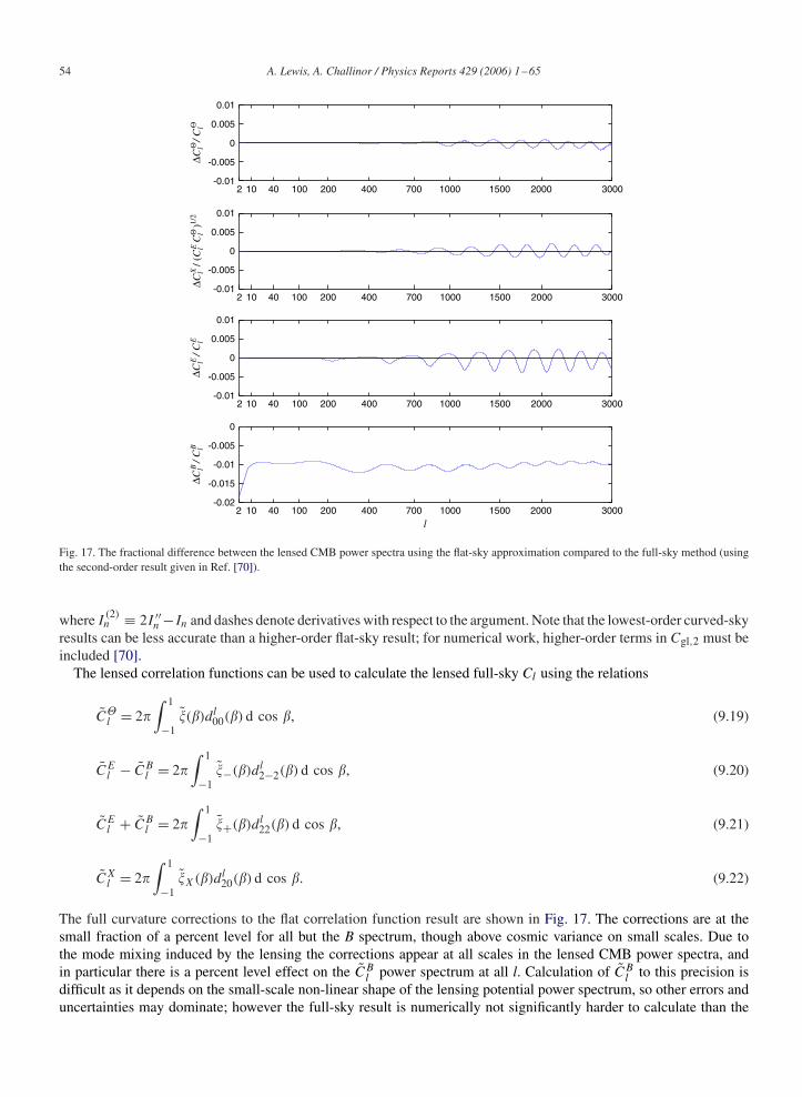
54 A. Lewis, A. Challinor / Physics Reports 429 (2006) 1 –65
2 10 40 100 200 400 700 1000 1500 2000 3000-0.01
-0.005
0
0.005
0.01
2 10 40 100 200 400 700 1000 1500 2000 3000-0.01
-0.005
0
0.005
0.01
2 10 40 100 200 400 700 1000 1500 2000 3000-0.01
-0.005
0
0.005
0.01
2 10 40 100 200 400 700 1000 1500 2000 3000-0.02
-0.015
-0.01
-0.005
0
l
∆Cl
/ Cl
ΘΘ
∆Cl
/ Cl
EE
∆Cl
/ Cl
BB
∆Cl
/ (C
l C
l )1/
2X
EΘ
Fig. 17. The fractional difference between the lensed CMB power spectra using the flat-sky approximation compared to the full-sky method (usingthe second-order result given in Ref. [70]).
where I(2)n ≡ 2I ′′
n −In and dashes denote derivatives with respect to the argument. Note that the lowest-order curved-skyresults can be less accurate than a higher-order flat-sky result; for numerical work, higher-order terms in Cgl,2 must beincluded [70].
The lensed correlation functions can be used to calculate the lensed full-sky Cl using the relations
Cl = 2
∫ 1
−1()dl
00() d cos , (9.19)
CEl − CB
l = 2∫ 1
−1−()dl
2−2() d cos , (9.20)
CEl + CB
l = 2∫ 1
−1+()dl
22() d cos , (9.21)
CXl = 2
∫ 1
−1X()dl
20() d cos . (9.22)
The full curvature corrections to the flat correlation function result are shown in Fig. 17. The corrections are at thesmall fraction of a percent level for all but the B spectrum, though above cosmic variance on small scales. Due tothe mode mixing induced by the lensing the corrections appear at all scales in the lensed CMB power spectra, andin particular there is a percent level effect on the CB
l power spectrum at all l. Calculation of CBl to this precision is
difficult as it depends on the small-scale non-linear shape of the lensing potential power spectrum, so other errors anduncertainties may dominate; however the full-sky result is numerically not significantly harder to calculate than the

A. Lewis, A. Challinor / Physics Reports 429 (2006) 1 –65 55
flat-sky approximation and hence should be used. It is included in the numerical CMB codes CAMB15 and CMBEASY.16
Note however that theoretical uncertainties in the recombination ionization history and various late-time secondariesare likely to be much more important than the sky-curvature correction.
Useful relations between full-sky and flat-sky harmonics and correlation functions are given in the appendices ofRefs. [110,128]. Most of the flat-sky results we have given in previous sections can be generalized to the full sky, e.g.the quadratic estimators for the potential [128] and results for the trispectrum structure [110].
10. Simulations
Simulating lensed CMB maps is straightforward in the lowest weak lensing approximation if both the lensingpotential and unlensed CMB fields are Gaussian and statistically isotropic: make two maps, one of the gradient of thelensing potential and one of the CMB, and a lensed map can then be made by remapping points on the CMB mapaccording to the deflection vectors =∇ from the lensing map using X(n)= X(n + ) [122,25,123]. The gradient ofthe deflection angle can be taken easily in harmonic space, then transformed to get maps of the x and y components. Inpractice the CMB map needs to be interpolated or generated at high resolution in order not to suffer from pixelizationissues when remapping the points.
On the full sky a pixel remapping scheme can also be used [134]. The deflection vector field can be constructed fromvector spherical harmonics (or equivalently spin −1 harmonics), and spherical trigonometry used to calculate the pixelremapping from the geodesic in the direction of the deflection vector. A parallelized code based on HEALPIX [147] ispublicly available.17 Simulating lensed skies is significantly slower than unlensed skies because of the higher resolutionrequired for the unlensed map, however it is efficiently parallelizable. Note that convolution with the observationalbeam takes place on the lensed sky, so for an accurate simulation the unlensed sky must be simulated at high resolutionindependent of the beam.
On smaller scales we may need to model the effects of non-linear evolution, perform ray-tracing to test the weaklensing approximations, and include other effects (such as SZ) in order to test their correlation and confusion with thelensing signal. In general this requires doing detailed numerical simulations for the density field [43,77,148–150] (fora recent review on N-body codes and references see e.g. Ref. [151]). The photon path can be computed by ray tracing,though in many cases the Born approximation can be used along an undeflected path to good accuracy to obtain resultswhich include just the non-linear physics.
11. Status and applications of CMB lensing
11.1. Observational status
At the time of writing there is no detection of lensing of the CMB or of lensing-induced cross-correlation withlarge scale structure [152]. This is expected to change very shortly, either by direct detection of the non-Gaussiansignature in the small-scale CMB, or by the improvement to model fitting by using the lensed as opposed to theunlensed CMB power spectra. Current data restrict the amplitude of the lensing effect to be within a factor of threeof the expected result, but consistent with zero. However lensing is a robust prediction, so in the next subsections wediscuss what new cosmological and/or astrophysical information we might be able to extract from future observations ofCMB lensing.
11.2. Cosmological model constraints
Cosmological parameter analyses using the lensed CMB power spectra (and ignoring the non-Gaussian structure) isstraightforward using standard Markov Chain Monte Carlo methods (e.g. using COSMOMC18 [153]), and will probably
15 http://camb.info16 http://cmbeasy.org17 http://cosmologist.info/lenspix/18 http://cosmologist.info/cosmomc/

56 A. Lewis, A. Challinor / Physics Reports 429 (2006) 1 –65
be adequate for the immediate future. Although the lensing effect on the power spectrum at l2000 is significant,the effect on recovered constraints of standard flat-universe cosmological parameters is mild [154,134]. For non-flatmodels the lensing signal can however be used to break the geometrical degeneracy, allowing a better CMB constrainton the curvature and dark energy [155].
With sensitive observations, information in the lensing potential can in principle be used to extract extra informationabout cosmological parameters. For example the unlensed CMB anisotropy is only weakly sensitive to neutrino massessufficiently light that they are relativistic at recombination. However the lensing potential probes later times, and thesmall scale damping effect on the lensing potential power spectrum can be significant. Ref. [156] finds that a neutrinowith mass 0.1 eV only changes the unlensed spectra at the sub-percent level, but the effect on the potential powerspectrum is ∼ 5%. If the lensing potential can be reconstructed to within this accuracy, this extra information canbe used to improve the limits on the neutrino mass from CMB data alone. Future experiments may ultimately beable to probe neutrino masses with error of ±0.035 eV [157]. Although probably not competitive with future Lyman-alpha and galaxy survey constraints, it is an independent check that is much less sensitive to non-linear evolution andbiasing issues.
The lensing potential is also a probe of the late-time evolution, and can be used to help constrain the dark energymodel. Cross-correlation of the lensing potential with the temperature can probe curvature and dark energy via theeffect on the large-scale ISW effect [97,100–102,104]. Further information can be extracted by using probes that aresensitive to somewhat different redshift ranges, for example galaxy weak lensing surveys [26,131]. Since the growthof large-scale perturbations is sensitive to the dark energy sound speed, cross-correlation studies may also provideconstraints on the dark energy clustering. Unfortunately cosmic variance dominates on the largest scales where thecross-correlations are significant, so the precision of the constraints is limited.
More direct constraints on the dark energy come from the angular and growth function effects on the lensing potentialpower spectrum [158]. The effect of massive neutrinos and details of the dark energy model (such as the equation ofstate) can be separated by differences in the scale-dependence of their effect on the lensing potential power spectrum[156]. This is illustrated for a flat universe in Fig. 18, which shows the fractional change when the equation of stateparameter w and neutrino mass are varied, but keeping the angular diameter distance to last scattering fixed. Thefiducial model is a cosmological constant model (w = −1) with massless neutrinos. These effects are, however, verynearly degenerate if only the lensed CMB power spectra are used: there is no angular scale for which the dominantcontribution is from the large-angle lenses for which the effects of massive neutrinos and changes in the dark energymodel are distinct [114]; see Fig. 18. Lensing potential reconstruction (or a full non-Gaussian likelihood analysis) isrequired to provide good non-degenerate constraints.
11.3. Cluster and galaxy mass
In Section 4 we discussed the effect of lensing on the statistics of the temperature power spectrum. On small scalesthe CMB has very little power, and what power there is comes mainly from the lensing signal from large scale structure(and other second-order effects). With very dense clumps of matter it may be possible to detect them individually viatheir lensing effect, hence the idea of using CMB lensing to learn about cluster and galaxy mass. Since lensing issensitive to the potential gradient, lensing constrains the projected mass distribution directly rather than most otherobservational signatures such as thermal SZ which are only sensitive to the baryonic component.
The small-scale unlensed CMB is very smooth due to diffusion damping, and can be locally approximated by agradient. Lensing makes photons appear to originate further from the centre of the cluster than they actually do, sothe cold side of the gradient will look hotter after lensing, and the hot side will look colder. This gives a distinc-tive ‘wiggle’ in the temperature in a direction aligned with the direction of the background CMB gradient. The ideais therefore to model these lensing wiggles in the observed temperature (and polarization) in an otherwise smoothunlensed background [73,159–161,150]. For a cluster deflection field (r), the wiggle due to the lensing is givensimply by (r) · ∇ in the gradient approximation. A particular example of the cluster lensing effect is shownin Fig. 19.
The rms temperature gradient is given by Eq. (4.17) and is ∼ 14 K/arcmin for standard models. Massive clusterscan give deflections of the order of an arcminute, so the lensing signal can be at the ∼ 10 K level. The scale ofthe dipole-like pattern induced by the cluster lensing is much smaller than the unlensed CMB, and so should inprinciple easily be observable for observations with high enough resolution and low enough noise. However the signal

A. Lewis, A. Challinor / Physics Reports 429 (2006) 1 –65 57
Fig. 18. Effect on lensing potential power spectrum (top) and lensed CMB spectra (bottom) of varying the neutrino mass (assumed the same for allthree families) and equation of state of dark energy at fixed angular diameter distance to last scattering in a flat model. The error boxes are cosmicvariance errors and ignore non-Gaussianity for the lensed CMB spectra.
depends on the background gradient, so only clusters in front of a significant gradient can have their mass constrainedthis way.
Note that in the central region of the cluster deflection angles can cross the centre, where the lensing is usually calledstrong lensing. The radius at which the deflections meet at a point in the centre is called the Einstein radius. Howevereven in the strong lensing region the deflection angles are still small, and the Born approximation should still be validfor a single thin lens, so this region can be handled in just the same way as the weak lensing signal at larger radii.
If the background gradient could be measured cleanly away from the cluster, the cluster deflection angles couldbe reconstructed directly from observations, and hence used to solve for the cluster profile and mass given certainassumptions. Unfortunately the situation is more complicated because the unlensed CMB is not exactly a gradient: thebackground gradient cannot be measured reliably far from the cluster due to small scale power in the CMB (as well asthe effect of lensing by the tails of the cluster). Fortunately the problem is statistically straightforward if we take theunlensed CMB field to be Gaussian: the correlation function of the observed temperature should just be given by the

58 A. Lewis, A. Challinor / Physics Reports 429 (2006) 1 –65
-3 -2 -1 0 1 2 3
-3
-2
-1
0
1
2
3
-100
-80
-60
-40
-20
0
20
40
60
80
100
-3 -2 -1 0 1 2 3 -3 -2 -1 0 1 2 3
-3
-2
-1
0
1
2
3
-100
-80
-60
-40
-20
0
20
40
60
80
100
-3
-2
-1
0
1
2
3
µ K
-10
-8
-6
-4
-2
0
2
4
6
8
10
Fig. 19. Simulated effect of cluster lensing on the CMB temperature. Left: the unlensed CMB; middle: the lensed CMB; right: the difference due tothe cluster lensing. The cluster is at redshift one, and has a spherically symmetric NFW profile with mass of m200 = 1015h−1M and concentrationparameter c = 5 (see Refs. [160,162]). Distances are in arcminutes, and can be compared to the cluster virial radius of 3.3 arcmin. In the middlefigure note the direction of the gradient inverts inside the ∼ 1 arcmin Einstein radius where the lensing deflections cross the centre of the cluster.This is a rather clean realization, in general the dipole pattern can be weaker and/or more complicated.
correlation function at the undeflected position on the last scattering surface. We can therefore work out the likelihoodof any given cluster deflection field () for some set of cluster parameters using
−2 log P(()|) = (xi)C−1(xi + i , xj + j )(xj ) + log |C(xi + i , xj + j )| (11.1)
in the absence of noise [162]. Here C is the covariance matrix given by the correlation function of the unlensed field,and noise can easily be included using the noise correlation function for the observed positions. The effect of lensingby other perturbations along the line of sight can be crudely modelled by using the lensed power spectrum, though amore careful analysis would require a study of the non-Gaussian distribution numerically using simulations.
This picture is complicated further by other secondary signals that cannot easily be distinguished from the lensingsignal. The effect of inhomogeneous kinetic SZ has been investigated from numerical simulations, and found to be amajor source of confusion in many cases [163,161]. Even in idealized cases the kinetic SZ signal can be important.For example if the cluster is rotating there will be a dipole-like signature that looks very like that expected from CMBlensing, and hence acts as a source of confusion [162] (though not aligned with the background gradient direction). TheOstriker–Vishniac and kinetic SZ signals from inhomogeneous reionization can also greatly increase the small scalepower in the unlensed CMB, adding an effective additional correlated noise. The moving lens effect (see Section 11.4)also introduces a dipole-like signal at the few K level for massive clusters [164,165]. However unlike the static lensingsignal this should be uncorrelated with the direction of the background CMB gradient, and is generally subdominantto fluctuations in the kinetic-SZ signal. Taken together these issues make it very challenging to obtain useful clusterconstraints from the CMB temperature, and certainly in the near future galaxy lensing is likely to be a much better wayto constrain cluster masses [162].
If information about the mass of lensing clusters can be obtained by other means (e.g. using SZ observations withsome assumptions), CMB lensing studies of many clusters can in principle be used to constrain cosmological parameters[163]. The complicating signals like kinetic-SZ would have to be distinguished, for example by using their correlationto the frequency-dependent thermal-SZ effect and different morphology [163,161]. Residual signals degrade the clusterlensing measurement and this is likely to be difficult in practice [150].
We might also want to attempt a general reconstruction of the projected density field of the cluster profile. Ref. [166]suggest a modification to the quadratic estimator potential reconstruction methods of Section 7 they claim is better oncluster scales, and obtained constraints on cluster masses by averaging over many clusters.
If there were sufficient small-scale structure in the CMB on cluster scales, e.g. due to secondary effects behind thecluster, these could also be used to measure the shear induced by the lens and hence used to constrain cluster massprofiles [122]. However this is likely to be difficult in practice as it requires very high resolution observations.
Cluster lensing techniques can in principle also be extended to galaxy CMB lensing [167], though the signal is muchsmaller (tenths of a micro-Kelvin) and arcsecond resolution is required. Cross-correlation of the CMB lensing signal

A. Lewis, A. Challinor / Physics Reports 429 (2006) 1 –65 59
with other sources can help to constrain cosmological parameters or learn about the source distributions, for examplecorrelation with the far-infrared background [168].
11.3.1. Cluster lensing of polarizationCluster lensing of the CMB polarization [162] is conceptually very similar to the temperature lensing, with potentially
two new gradients in Q and U (only correlated at the 10% level with the temperature gradient). The rms gradient of theStokes’parameters is ∼ 1 K/arcmin, so a signal ∼ 1 K is expected from massive clusters. Detection therefore requiresnoise levels about ten times lower than for the temperature. If the temperature signal could be used at this sensitivitylevel the temperature constraints would always be much better. However, as mentioned above, the temperature signalis complicated by confusion due to kinetic SZ (and other signals). By contrast the polarization signal is expected to berelatively clean [169–172,81]. Since there are both Q and U Stoke’s parameters there are also effectively two randomgradients to play with, so polarization cluster constraints suffer less from random variations in the gradient beinglensed. Furthermore lensing of a temperature gradient cannot be used to detect deflections orthogonal to the gradient,but with the two Stokes’ parameter gradients this degeneracy can in general be broken: polarization cluster lensingshould therefore be useful to improve general profile reconstruction.
In a fixed flat sky basis, using the gradient approximation, some deflection field (r) gives the lensed polarizationfield
P (r) = P(r) + (r) · ∇P , (11.2)
where as usual P ≡ Q + iU . A constant gradient is neither E nor B, because making the E/B decomposition locallyrequires taking two gradients (see Section 5). Using the definition of the harmonic components in Eqs. (5.22), andassuming a suitably well behaved deflection field, the lensed components are
E(l) = −(l) · (cos(2l)∇Q + sin(2l)∇U),
B(l) = −(l) · (− sin(2l)∇Q + cos(2l)∇U). (11.3)
At a point the gradients of Q and U are uncorrelated, and averaging over (assumed Gaussian) background polarizationgradients we get
〈|E(l)|2〉∇P = 12RE |(l)|2,
〈|B(l)|2〉∇P = 12RE |(l)|2, (11.4)
where RE = 〈|∇Q|2〉 = 〈|∇U |2〉 as in Eq. (5.37). An arbitrary deflection field therefore gives identical E and B modeson average when lensing a pure gradient field. Taking the average over a Gaussian deflection field gives the result wefound previously in Eqs. (5.35) and (5.36). If the deflection field has circular symmetry (as from a spherical cluster),the angular average of the E and B mode power are equal for any fixed polarization gradient:
1
2
∫dl |E(l)|2 = 2(l)
4(|∇Q|2 + |∇U |2),
1
2
∫dl |B(l)|2 = 2(l)
4(|∇Q|2 + |∇U |2). (11.5)
Cluster lensing therefore generates equal amplitude E and B in the gradient approximation [162]. However there is verylittle power in the unlensed E or B polarization on cluster scales, so the lensed E contains almost as much informationas the lensed B: the E/B decomposition is not as useful as on larger scales. If the full likelihood function is used there isin fact no need to use E and B, the correlation function can be calculated directly for the Q and U Stoke’s parameters,and the likelihood calculated using the analogue of Eq. (11.1). However for nearby large clusters the B mode signalmay allow the cluster signal to be distinguished from unlensed CMB ‘noise’, so unlike in the temperature case clusterlensing may not be CMB noise limited for large cluster sizes.
Observations of CMB lensing by clusters can be used to constrain the masses of clusters at any redshift. For the bulk ofclusters at redshift z1 mass measurements using lensed galaxy shears are however likely to be much better [162], even

60 A. Lewis, A. Challinor / Physics Reports 429 (2006) 1 –65
allowing for very optimistic future CMB observations. For high-redshift clusters, for which there are very few sourcegalaxies that can be used for shear measurements, CMB lensing may however be a better way to constrain the mass ifhigh sensitivity measurements of a clean polarization signal are available. The largest identified sources of confusionare likely to be re-scattering from anisotropic thermal-SZ giving a frequency-dependent cluster polarization signal0.7 K [173,172], and cluster-scattering of the CMB quadrupole giving a frequency-independent signal 0.1 K[174–176]. However only dipole-like components should confuse the lensing signal of the cluster mass.
11.4. Moving lenses and dipole lensing
If a lensing mass is moving with respect to the CMB it corresponds to an evolving potential well that inducesanisotropies in a manner similar to the ISW and Rees–Sciama effects. If a lens is moving transverse to the line of sight,a photon passing the front side of the lens (with respect to the direction of motion) will see a weaker potential on itsway into the lens than on the way out, and hence receives a net redshift. Similarly a photon on the other side will receivea net blue shift. The moving lens therefore induces a dipole-like temperature anisotropy in the photons crossing thelens’ path [164,177]. For small transverse 3-velocity v⊥ (natural units), the temperature anisotropy induced by a smallmoving lens is at lowest order
= −2
∫d v⊥ · ∇⊥ = v⊥ · , (11.6)
where the integral is along the photon path, v⊥ is transverse to the line of sight and is the deflection angle of thephoton at the lens (related to the observed deflection angle by the ratio of the relevant angular diameter distances). Thesignature from a cluster is therefore rather similar to that coming from the lensing of the background CMB temperaturegradient, with the difference that here the dipole pattern is aligned with the transverse velocity of the cluster ratherthan the background gradient. For a 1015h−1M mass cluster moving transverse to the line of sight at 600 km s−1 theamplitude of the signal is ∼ 5 × 10⁻⁷, corresponding to a signal of ∼ 1 K. It is therefore generally subdominant tothe effect of lensing of the background CMB gradient.
As described above in the rest frame of the CMB the moving lens contribution is not really a lensing effect, but acontribution to the Rees–Sciama effect [82] (the other contributions being due to the rest-frame change in the lensingmass’ potential with time). However in the rest frame of the lens the moving lens effect can be interpreted as CMBdipole lensing, as follows. The velocity of the lens relative to the rest frame of the CMB induces a dipole in the lens’frame so that the temperature coming from direction r is (1 + v · r) at lowest order. In its rest frame, the static lensdeflects the photon by an angle perpendicular to the line of sight n, so the observed temperature along this directionis [1 + v · (n + )]. Transforming back to the original frame, we have a temperature anisotropy = v⊥ · .On the back side the photons are deflected from the hot side of the dipole so they are hotter that they would have beenwithout the deflection. On the other side they are colder. This temperature anisotropy is exactly the same pattern wecalculated above, so dipole lensing is an equally valid way to interpret the signal.
What happens if we change our velocity to be comoving with the lens? In this frame the lens is at rest, but ourobserved CMB has a dipole. We might therefore think that we could compute ∇ · ∇ to get the contribution fromCMB lensing by the cluster. This however gives a different answer in general: the lensing potential depends on thedistance to the cluster and source via the angular 1−/∗ factor, whereas the effect we computed above is independentof distance. This is essentially because the relevant dipole is the one seen by the lens, not the one seen by us. It istherefore not valid to consider the dipole due to our local motion as a dipole source at last scattering that is then deflectedby the lens [178]. The velocity dipole source must be taken to be at infinite distance to get a consistent answer. Theprimordial dipole at last scattering is however lensed, and is physically distinct from the local motion-induced dipole(which is also associated with other higher order signals arising from the transformation from the CMB frame [52];see Section 2.3).
Typical peculiar velocities are O(10−3c), and the moving-lens signature could, in principle, be used to measure thetransverse component. However this may well be impossible in practice due to confusion with other larger signals[179,165,180]. The moving-lens signal itself is also a potential source of confusion when trying to measure clusterproperties from CMB lensing as it gives a similar dipole-like pattern, albeit uncorrelated with the background gradient.
There will also be some local effect due to our local mass distribution moving relative to the CMB, giving a localcontribution to the large-scale CMB anisotropies [181]. This effect is however probably very small [178].

A. Lewis, A. Challinor / Physics Reports 429 (2006) 1 –65 61
An interesting example of a moving-lens effect is the signal generated by any cosmic strings that may be presentwithin our horizon volume (for a review see e.g. Ref. [182]). A cosmic string with tension (energy per length) alters the surrounding geometry by a deficit angle 8G . This gives an effective rest-frame deflection angle = 4G for lines of sight perpendicular to the string. The deflection angle is small for models consistent withcurrent observations (10−4) and likely to be significantly smaller, so the signal from lensing of CMB anisotropiesis small. However for strings moving close to the speed of light, this should induce temperature fluctuations / ∼4G with a step-like discontinuity across the string. This is called the (Gott-)Kaiser–Stebbins effect [183,184] andacts in addition to the signal generated from string-induced perturbations at last scattering. The Kaiser–Stebbins ef-fect can also be understood in the CMB frame in terms of integrated anisotropy from the scalar, vector and tensorperturbations that the moving string generates. It may be possible to detect this cosmic-string imprint in future high-resolution data using its distinct non-Gaussian character; see Ref. [185] for a targeted search and constraints withWMAP data.
Finally, if a lens is moving along the line of sight the deflection angle calculated in the rest frame acquires a O(v · n/c)
correction when transformed back to the CMB frame. This is generally totally negligible [186], and can be consistentlyneglected in any lowest-order weak lensing calculation for O(10−3c) velocities.
12. Summary and outlook
It is a general prediction of metric theories of gravity that gravitational lensing must occur. It is therefore a robustprediction that the CMB must be lensed by potential gradients along the line of sight. As we have seen, this weaklensing of the CMB has several important observable effects, most of which are now well understood theoretically instandard models. In summary the lensing:
• Perturbs the observed position of the points on the last scattering surface without changing the frequency dependenceso the spectrum remains blackbody.
• Can be modelled accurately using an integrated lensing potential that is only weakly sensitive to non-linear structureson scales above tens of arcminutes.
• Smooths out the acoustic oscillations in the temperature, E-polarization and cross-power spectra by several percent.• Generates B-mode polarization at the K level by lensing of E-polarization. This is a potential source of confusion for
detecting primordial gravitational waves. A significant fraction of the lens-induced B-modes come from small-scalelenses and the non-linear density field introduces ∼ 10% corrections to the B-mode power on all scales.
• Produces a distinctive small-scale non-Gaussian trispectrum (four-point function), with smaller signals in the highereven n-point functions.
• Introduces no non-Gaussian signals in the small-scale odd n-point functions if small-scale correlations between thelensing potential and e.g. kinetic-SZ are neglected.
• Introduces a large-scale non-Gaussian bispectrum (three-point function) due to correlation between the lensingpotential and large-scale temperature.
• Can in principle be delensed by using high-resolution polarization observations to reconstruct the lensing potentialand re-mapping points to the last scattering surface.
• Can be used to improve constraints on some cosmological parameters that are poorly constrained by the CMB powerspectra alone, such as the dark energy model and sub-eV neutrino masses.
• Can be simulated accurately in the Gaussian limit, and also from N-body simulation for more realistic small-scaleanalyses.
• May be able to constrain the mass distribution of high-redshift clusters from their lensing signature observed athigh-resolution and sensitivity.
At the time of writing there is no detection of the lensing signal, though this is expected to change fairly soon.CMB observations are already at the level of precision where the lensing effect on the temperature power spectramust shortly be included for an accurate analysis. This will certainly be the case once data from the future Plancksatellite,19 currently scheduled for launch in early 2008, becomes available [134]. Polarization experiments already
19 http://www.rssd.esa.int/index.php?project = Planck.

62 A. Lewis, A. Challinor / Physics Reports 429 (2006) 1 –65
taking data, most notably QUAD,20 have the sensitivity to detect the B-modes due to lensing after ∼ one year ofintegration. The next generation of polarization experiments targeting B-modes from gravitational waves, such asClover21 and QUIET,22 are being designed so that lens-induced B-modes are the limiting source of confusion fordetecting primary B-modes from gravity waves (assuming foreground subtraction is efficient). For such instruments,lensing reconstruction and delensing will start to become beneficial. Proposed future missions such as the InflationProbe23 (CMBpol) would be able to measure the lensed B-mode signal at high precision, and delensing (or a fulllikelihood analysis) will become essential to place good constraints on primordial gravity waves.
Although CMB lensing is generally well understood, there remain areas for further work. In particular the delensingmethods for subtracting out the B-mode lensing signal have so far only been developed in idealized cases (flat skywithout boundaries, simple noise and beam properties, no non-linear structures, etc.). There are also no known generalmethods for performing a full accurate parameter likelihood analysis on lensed data once simple approximations are nolonger good enough. Such methods may be required to obtain accurate parameter constraints from future high-resolutionmeasurements of the E (and B) polarization. In principle, a near-optimal likelihood analysis would additionally be ableto constrain the gravity waves without a separate explicit delensing step. Analysis of the observed temperature field onsmall scales will require accurate modelling of kinetic-SZ and other non-linear signals, including correlations with thelensing signal. It may also be important to account for lensing in non-standard models, for example when trying to findmatched circles from non-trivial topologies. If the primordial fluctuations turn out to be significantly non-Gaussian oranisotropic this will also significantly complicate the full lensed analysis and require much further work.
Acknowledgements
We thank Chris Hirata, Wayne Hu, and Oliver Zahn for figures and data. AL acknowledges a PPARC Advancedfellowship and AC a Royal Society University Research Fellowship. The Beowulf cluster used for some calculationswas funded by the Canada Foundation for Innovation and the Ontario Innovation Trust.
References
[1] A. Liddle, D. Lyth, Cosmological Inflation and Large-Scale Structure, Cambridge University Press, Cambridge, 2000 [ISBN: 052166022X].[2] W. Hu, S. Dodelson, Ann. Rev. Astron. Astrophys. 40 (2002) 171 [astro-ph/0110414].[3] W. Hu, Ann. Phys. 303 (2003) 203 [astro-ph/0210696].[4] S. Dodelson, Modern Cosmology, Academic Press, New York, 2003 [ISBN: 0122191412].[5] W. Hu, M. White, Sci. Am. 290 (2004) 44 [http://background.uchicago.edu/∼whu/Papers/HuWhi04.pdf].[6] A. Challinor, (2004), [astro-ph/0403344].[7] D. Scott, G. Smoot, (2006), [astro-ph/0601307].[8] T. Padmanabhan, (2006), [astro-ph/0602117].[9] A. Blanchard, J. Schneider, Astron. Astrophys. 184 (1987) 1.
[10] S. Cole, G. Efstathiou, Mon. Not. Roy. Astron. Soc. 239 (1989) 195.[11] E.V. Linder, Mon. Not. Roy. Astron. Soc. 243 (1990) 353.[12] U. Seljak, Astrophys. J. 463 (1996) 1 [astro-ph/9505109].[13] R.B. Metcalf, J. Silk, Astrophys. J. 489 (1997) 1 [astro-ph/9708059].[14] C.L. Bennett, et al., Astrophys. J. Lett. 464 (1996) L1 [astro-ph/9601067].[15] D.N. Spergel, et al., Astrophys. J. 148 (Suppl.) (2003) 175 [astro-ph/0302209].[16] R. Sachs, A. Wolfe, Astrophys. J. 147 (1967) 735.[17] M.J. Rees, Astrophys. J. 153 (1968) L1+.[18] A.G. Polnarev, Sov. Astron. 29 (1985) 607.[19] W. Hu, M.J. White, New Astron. 2 (1997) 323 [astro-ph/9706147].[20] R. Sunyaev, Y. Zel’dovich, Comm. Astrophys. Sp. Phys. 4 (1972) 173.[21] A. Cooray, D. Baumann, K. Sigurdson, (2004), [astro-ph/0410006].[22] X.P. Wu, Mon. Not. Roy. Astron. Soc. 349 (2004) 816 [astro-ph/0312469].[23] V. Perlick, Living Rev. Relativity 7 (2004) [http://www.livingreviews.org/lrr-2004-9].[24] M. Bartelmann, P. Schneider, Phys. Rep. 340 (2001) 291 [astro-ph/9912508].[25] F. Bernardeau, Astron. Astrophys. 338 (1998) 767 [astro-ph/9802243].
20 http://www.astro.cf.ac.uk/groups/instrumentation/projects/quad/21 http://www.astro.cf.ac.uk/groups/instrumentation/projects/clover/22 http://quiet.uchicago.edu/23 http://universe.nasa.gov/program/inflation.html

A. Lewis, A. Challinor / Physics Reports 429 (2006) 1 –65 63
[26] L.V. van Waerbeke, F. Bernardeau, K. Benabed, Astrophys. J. 540 (2000) 14 [astro-ph/9910366].[27] C.M. Hirata, U. Seljak, Phys. Rev. D 68 (2003) 083002 [astro-ph/0306354].[28] C. Shapiro, A. Cooray, (2006), [astro-ph/0601226].[29] D.E. Holz, R.M. Wald, Phys. Rev. D 58 (1998) 063501 [astro-ph/9708036].[30] G.F.R. Ellis, B.A. Bassett, P.K.S. Dunsby, Class. Quant. Grav. 15 (1998) 2345 [gr-qc/9801092].[31] R. Lieu, J.P.D. Mittaz, Astrophys. J. 623 (2004) L1 [astro-ph/0409048].[32] C.C. Dyer, R.C. Roeder, Astrophys. J. 174 (1972) L115+.[33] S. Weinberg, Astrophys. J. 208 (1976) L1.[34] J.A. Peacock, Mon. Not. Roy. Astron. Soc. 223 (1986) 113.[35] T.W.B. Kibble, R. Lieu, Astrophys. J. 632 (2005) 718 [astro-ph/0412275].[36] T. Fukushige, J. Makino, T. Ebisuzaki, Astrophys. J. 436 (1994) L107 [astro-ph/9409069].[37] R. Lieu, J.P.D. Mittaz, Astrophys. J. 628 (2005) 583 astro-ph/0412276.[38] S. Seitz, P. Schneider, J. Ehlers, Class. Quant. Grav. 11 (1994) 2345 [astro-ph/9403056].[39] T. Hamana, et al., Mon. Not. Roy. Astron. Soc. 356 (2005) 829 [astro-ph/0407599].[40] P. Schneider, J. Ehlers, E. Falco, Gravitational Lenses, Springer, Berlin, 1992 [ISBN: 0387970703].[41] A.O. Petters, H. Levine, J. Wambsganss, Singularity Theory and Gravitational Lensing, Birkhäuser, Boston, 2001 [ISBN: 0817636684].[42] S. Mollerach, E. Roulet, Gravitational Lensing and Microlensing, World Scientific, Singapore, 2002 [ISBN: 9810248520].[43] B. Jain, U. Seljak, S.D.M. White, Astrophys. J. 530 (2000) 547 [astro-ph/9901191].[44] N. Kaiser, A.H. Jaffe, Astrophys. J. 484 (1997) 545 [astro-ph/9609043].[45] S. Dodelson, E. Rozo, A. Stebbins, Phys. Rev. Lett. 91 (2003) 021301 [astro-ph/0301177].[46] W. Hu, A. Cooray, Phys. Rev. D 63 (2001) 023504 [astro-ph/0008001].[47] N. Kaiser, Astrophys. J. 498 (1998) 26 [astro-ph/9610120].[48] R.D. Blandford, et al., Mon. Not. Roy. Astron. Soc. 251 (1991) 600.[49] R.R. Wald, General Relativity, University of Chicago Press, Chicago, 1984 [ISBN: 0226870332].[50] L. Van Waerbeke, Y. Mellier, (2003), [astro-ph/0305089].[51] R. Sachs, Proc. Roy. Soc. Lon. 264 (1961) 309.[52] A. Challinor, F. van Leeuwen, Phys. Rev. D 65 (2002) 103001 [astro-ph/0112457].[53] M. Kamionkowski, L. Knox, Phys. Rev. D 67 (2003) 063001 [astro-ph/0210165].[54] C. Gordon, A. Lewis, Phys. Rev. D 67 (2003) 123513 [astro-ph/0212248].[55] D. Menzies, G.J. Mathews, Astrophys. J. 624 (2005) 7 [astro-ph/0409175].[56] W.R. Stoeger, G.F.R. Ellis, C. Xu, Phys. Rev. D 49 (1994) 1845.[57] C.W. Misner, K.S. Thorne, J.A. Wheeler, Gravitation, Freeman, New York, 1973 [ISBN: 0716703440].[58] A. Challinor, Phys. Rev. D 62 (2000) 043004 [astro-ph/9911481].[59] A. Cooray, M. Kamionkowski, R.R. Caldwell, Phys. Rev. D 71 (2005) 123527 [astro-ph/0503002].[60] S. Dodelson, et al., Phys. Rev. D 72 (2005) 103004 [astro-ph/0503160].[61] A. Cooray, W. Hu, Astrophys. J. 574 (2002) 19 [astro-ph/0202411].[62] V. Acquaviva, C. Baccigalupi, F. Perrotta, Phys. Rev. D 70 (2004) 023515 [astro-ph/0403654].[63] J.D. Bekenstein, Phys. Rev. D 70 (2004) 083509 [astro-ph/0403694].[64] H.S. Zhao, et al., (2005), [astro-ph/0509590].[65] R.E. Smith, et al., The virgo consortium, Mon. Not. Roy. Astron. Soc. 341 (2003) 1311 [astro-ph/0207664].[66] A. Lewis, A. Challinor, A. Lasenby, Astrophys. J. 538 (2000) 473 [astro-ph/9911177].[67] W. Hu, Phys. Rev. D 62 (2000) 043007 [astro-ph/0001303].[68] E.V. Linder, Astron. Astrophys. 323 (1997) 305 [astro-ph/9606141].[69] P. McDonald, H. Trac, C. Contaldi, MNRAS 366 (2006) 547 [astro-ph/0505565].[70] A. Challinor, A. Lewis, Phys. Rev. D 71 (2005) 103010 [astro-ph/0502425].[71] K.S. Mandel, M. Zaldarriaga, (2005), [astro-ph/0512218].[72] A.R. Cooray, New Astron. 9 (2004) 173 [astro-ph/0309301].[73] M. Zaldarriaga, Phys. Rev. D 62 (2000) 063510 [astro-ph/9910498].[74] U. Seljak, M. Zaldarriaga, Astrophys. J. 469 (1996) 437 [astro-ph/9603033].[75] M. Doran, J. Chem. Appl. Phys. 0510 (2005) 011 [astro-ph/0302138].[76] O. Zahn, et al., Astrophys. J. 630 (2005) 657 [astro-ph/0503166].[77] A. Amblard, C. Vale, M.J. White, New Astron. 9 (2004) 687 [astro-ph/0403075].[78] M.G. Santos, et al., Astrophys. J. 598 (2003) 756 [astro-ph/0305471].[79] W. Hu, M.J. White, Astron. Astrophys. 315 (1996) 33 [astro-ph/9507060].[80] L. Knox, R. Scoccimarro, S. Dodelson, Phys. Rev. Lett. 81 (1998) 2004 [astro-ph/9805012].[81] W. Hu, Astrophys. J. 529 (2000) 12 [astro-ph/9907103].[82] M.J. Rees, D.W. Sciama, Nature 217 (1968) 511.[83] U. Seljak, Astrophys. J. 460 (1996) 549 [astro-ph/9506048].[84] U. Seljak, Astrophys. J. 436 (1994) 509 [astro-ph/9405002].[85] A. Lewis, A. Challinor, N. Turok, Phys. Rev. D 65 (2002) 023505 [astro-ph/0106536].[86] E.F. Bunn, et al., Phys. Rev. D 67 (2003) 023501 [astro-ph/0207338].[87] A. Lewis, Phys. Rev. D 68 (2003) 083509 [astro-ph/0305545].

64 A. Lewis, A. Challinor / Physics Reports 429 (2006) 1 –65
[88] M. Kamionkowski, A. Kosowsky, A. Stebbins, Phys. Rev. D 55 (1997) 7368 [astro-ph/9611125].[89] M. Zaldarriaga, U. Seljak, Phys. Rev. D 55 (1997) 1830 [astro-ph/9609170].[90] M. Zaldarriaga, U. Seljak, Phys. Rev. D 58 (1998) 023003 [astro-ph/9803150].[91] C.J. MacTavish et al. (2005), [astro-ph/0507503].[92] U. Seljak, M. Zaldarriaga, Phys. Rev. Lett. 78 (1997) 2054 [astro-ph/9609169].[93] V. Mukhanov, H. Feldman, R. Brandenberger, Phys. Rep. 215 (1992) 203.[94] P.J. Steinhardt, N. Turok, Phys. Rev. D 65 (2002) 126003 [hep-ph/0111098].[95] A. Linde, V. Mukhanov, M. Sasaki, J. Chem. Appl. Phys. 0510 (2005) 002 [astro-ph/0509015].[96] A.A. Starobinskii, JETP Lett. 30 (1979) 682.[97] W. Hu, Phys. Rev. D 65 (2002) 023003 [astro-ph/0108090].[98] M. Amarie, C. Hirata, U. Seljak, Phys. Rev. D 72 (2005) 123006 [astro-ph/0508293].[99] A. Cooray, Phys. Rev. D 64 (2001) 063514 [astro-ph/0105063].
[100] U. Seljak, M. Zaldarriaga, Phys. Rev. D 60 (1999) 043504 [astro-ph/9811123].[101] D.M. Goldberg, D.N. Spergel, Phys. Rev. D 59 (1999) 103002 [astro-ph/9811251].[102] F. Giovi, C. Baccigalupi, F. Perrotta, Phys. Rev. D 68 (2003) 123002 [astro-ph/0308118].[103] F. Giovi, C. Baccigalupi, F. Perrotta, Phys. Rev. D 71 (2005) 103009 [astro-ph/0411702].[104] B. Gold, Phys. Rev. D 71 (2005) 063522 [astro-ph/0411376].[105] U.L. Pen, et al., Astrophys. J. 592 (2003) 664 [astro-ph/0302031].[106] A. Cooray, W. Hu, Astrophys. J. 548 (2001) 7 [astro-ph/0004151].[107] E. Komatsu, D.N. Spergel, Phys. Rev. D 63 (2001) 063002 [astro-ph/0005036].[108] M.H. Kesden, A. Cooray, M. Kamionkowski, Phys. Rev. D 66 (2002) 083007 [astro-ph/0208325].[109] F. Bernardeau, Astron. Astrophys. 324 (1997) 15 [astro-ph/9611012].[110] W. Hu, Phys. Rev. D 64 (2001) 083005 [astro-ph/0105117].[111] S. Winitzki, (1998), [astro-ph/9806105].[112] T. Okamoto, W. Hu, Phys. Rev. D 66 (2002) 063008 [astro-ph/0206155].[113] K.M. Smith, W. Hu, M. Kaplinghat, Phys. Rev. D 70 (2004) 043002 [astro-ph/0402442].[114] S. Smith, A. Challinor, G. Rocha, Phys. Rev. D 73 (2006) 023517 [astro-ph/0511703].[115] J.M. Bardeen, et al., Astrophys. J. 304 (1986) 15.[116] J.R. Bond, G. Efstathiou, Mon. Not. Roy. Astron. Soc. 226 (1987) 655.[117] M. Takada, E. Komatsu, T. Futamase, Astrophys. J. 533 (2000) L83 [astro-ph/9908284].[118] M. Takada, Astrophys. J. 558 (2001) 29 [astro-ph/0101449].[119] J. Lesgourgues, et al., Phys. Rev. D 71 (2005) 103514 [astro-ph/0412551].[120] T. Brunier, F. Bernardeau, (2006), [astro-ph/0602276].[121] D. Babich, M. Zaldarriaga, Phys. Rev. D 70 (2004) 083005 [astro-ph/0408455].[122] M. Zaldarriaga, U. Seljak, Phys. Rev. D 59 (1999) 123507 [astro-ph/9810257].[123] W. Hu, Astrophys. J. 557 (2001) L79 [astro-ph/0105424].[124] A. Cooray, Phys. Rev. D 66 (2002) 103509 [astro-ph/0205306].[125] K. Sigurdson, A. Cooray, Phys. Rev. Lett. 95 (2005) 211303 [astro-ph/0502549].[126] O. Zahn, M. Zaldarriaga, (2005), [astro-ph/0511547].[127] W. Hu, T. Okamoto, Astrophys. J. 574 (2002) 566 [astro-ph/0111606].[128] T. Okamoto, W. Hu, Phys. Rev. D 67 (2003) 083002 [astro-ph/0301031].[129] A. Cooray, M. Kesden, New Astron. 8 (2003) 231 [astro-ph/0204068].[130] M. Kesden, A. Cooray, M. Kamionkowski, Phys. Rev. D 67 (2003) 123507 [astro-ph/0302536].[131] K. Benabed, F. Bernardeau, L. van Waerbeke, Phys. Rev. D 63 (2001) 043501 [astro-ph/0003038].[132] J. Guzik, U. Seljak, M. Zaldarriaga, Phys. Rev. D 62 (2000) 043517 [astro-ph/9912505].[133] C.M. Hirata, U. Seljak, Phys. Rev. D 67 (2003) 043001 [astro-ph/0209489].[134] A. Lewis, Phys. Rev. D 71 (2005) 083008 [astro-ph/0502469].[135] W. Hu, T. Okamoto, Phys. Rev. D 69 (2004) 043004 [astro-ph/0308049].[136] L. Knox, Y.S. Song, Phys. Rev. Lett. 89 (2002) 011303 [astro-ph/0202286].[137] M. Kesden, A. Cooray, M. Kamionkowski, Phys. Rev. Lett. 89 (2002) 011304 [astro-ph/0202434].[138] U. Seljak, C.M. Hirata, Phys. Rev. D 69 (2004) 043005 [astro-ph/0310163].[139] W. Hu, M.M. Hedman, M. Zaldarriaga, Phys. Rev. D 67 (2003) 043004 [astro-ph/0210096].[140] M. Tucci, et al., Mon. Not. Roy. Astron. Soc. 360 (2005) 926 [astro-ph/0411567].[141] L. Verde, H. Peiris, R. Jimenez, J. Chem. Appl. Phys. 0601 (2006) 019 [astro-ph/0506036].[142] B.D. Wandelt, D.L. Larson, A. Lakshminarayanan, Phys. Rev. D 70 (2004) 083511 [astro-ph/0310080].[143] A. Challinor, G. Chon, Phys. Rev. D 66 (2002) 127301 [astro-ph/0301064].[144] U. Seljak, et al., Phys. Rev. D 68 (2003) 083507 [astro-ph/0306052].[145] D.M. Brink, G.R. Satchler, Angular Momentum, third ed., Clarendon Press, Oxford, 1993 [ISBN: 0198517599].[146] D.A. Varshalovich, A.N. Moskalev, V.K. Khersonskii, Quantum Theory of Angular Momentum, Word Scientific, Singapore, 1988 [ISBN:
9971509962].[147] K.M. Gorski, et al., Astrophys. J. 622 (2005) 759 [astro-ph/0409513].[148] M.J. White, W. Hu, Astrophys. J. 537 (2000) 1 [astro-ph/9909165].

A. Lewis, A. Challinor / Physics Reports 429 (2006) 1 –65 65
[149] L. Anton, et al., Astrophys. J. 628 (2005) 1 [astro-ph/0504448].[150] C. Vale, A. Amblard, M.J. White, New Astron. 10 (2004) 1 [astro-ph/0402004].[151] K. Heitmann, et al., Astrophys. J. 160 (Suppl.) (2005) 28 [astro-ph/0411795].[152] C.M. Hirata, et al., Phys. Rev. D 70 (2004) 103501 [astro-ph/0406004].[153] A. Lewis, S. Bridle, Phys. Rev. D 66 (2002) 103511 [astro-ph/0205436].[154] M. Zaldarriaga, D.N. Spergel, U. Seljak, Astrophys. J. 488 (1997) 1 [astro-ph/9702157].[155] R. Stompor, G. Efstathiou, Mon. Not. Roy. Astron. Soc. 302 (1999) 735 [astro-ph/9805294].[156] M. Kaplinghat, L. Knox, Y.S. Song, Phys. Rev. Lett. 91 (2003) 241301 [astro-ph/0303344].[157] J. Lesgourgues, et al., Phys. Rev. D 73 (2006) 045021 [astro-ph/0511735].[158] V. Acquaviva, C. Baccigalupi, (2005), [astro-ph/0507644].[159] U. Seljak, M. Zaldarriaga, Astrophys. J. 538 (2000) 57 [astro-ph/9907254].[160] S. Dodelson, Phys. Rev. D 70 (2004) 023009 [astro-ph/0402314].[161] G.P. Holder, A. Kosowsky, Astrophys. J. 616 (2004) 8 [astro-ph/0401519].[162] A. Lewis, L. King, Phys. Rev. D 73 (2006) 063006 [astro-ph/0512104].[163] A.R. Cooray, Astrophys. J. 596 (2003) L127 [astro-ph/0305515].[164] M. Birkinshaw, S.F. Gull, Nature 302 (1983) 315.[165] N. Aghanim, et al., Astron. Astrophys. 334 (1998) 409 [astro-ph/9803040].[166] M. Maturi, et al., Astron. Astrophys. 436 (2005) 37 [astro-ph/0408064].[167] S. Dodelson, G.D. Starkman, (2003), [astro-ph/0305467].[168] Y.S. Song, et al., Astrophys. J. 590 (2003) 664 [astro-ph/0209001].[169] P. Valageas, A. Balbi, J. Silk, Astron. Astrophys. 367 (2001) 1 [astro-ph/0009040].[170] M. Gibilisco, Astrophys. Space Sci. 249 (1997) 189 [astro-ph/9701203].[171] A. Challinor, M. Ford, A. Lasenby, Mon. Not. Roy. Astron. Soc. 312 (2000) 159 [astro-ph/9905227].[172] M. Shimon et al., (2006), [astro-ph/0602528].[173] G. Lavaux, et al., Mon. Not. Roy. Astron. Soc. 347 (2004) 729 [astro-ph/0307293].[174] M. Kamionkowski, A. Loeb, Phys. Rev. D 56 (1997) 4511 [astro-ph/9703118].[175] A. Cooray, D. Baumann, Phys. Rev. D 67 (2003) 063505 [astro-ph/0211095].[176] A. Amblard, M.J. White, New Astron. 10 (2005) 417 [astro-ph/0409063].[177] L.I. Gurvits, I.G. Mitrofanov, Nature 324 (1986) 349.[178] A. Cooray, N. Seto, J. Chem. Appl. Phys. 0512 (2005) [astro-ph/0510137].[179] R. Tuluie, P. Laguna, Astrophys. J. 445 (1995) L73 [astro-ph/9501059].[180] A. Cooray, Phys. Rev. D 65 (2002) 083518 [astro-ph/0109162].[181] C. Vale, (2005), [astro-ph/0509039].[182] A. Vilenkin, E. Shellard, Cosmic Strings and Other Topological Defects, CUP, 2000, [ISBN: 0521654769].[183] N. Kaiser, A. Stebbins, Nature 310 (1984) 391.[184] J.R. Gott, Astrophys. J. 288 (1985) 422.[185] A.S. Lo, E.L. Wright, (2005), [astro-ph/0503120].[186] B.M. Schaefer, M. Bartelmann, (2005), [astro-ph/0502208].