weak-strong uniqueness for heat conducting non-newtonian
TRANSCRIPT

arX
iv:2
109.
1063
6v1
[m
ath.
AP]
22
Sep
2021
Weak-strong Uniqueness for Heat Conducting
non-Newtonian Incompressible Fluids ⋆
Pablo Alexei Gazca-Orozco, Victoria Patel
aDepartment of Data Science, FAU Erlangen-Nurnberg, Cauerstraße
11, 91058, Erlangen, GermanybMathematical Institute, University of Oxford, Andrew Wiles Building, Woodstock
Road, Oxford, OX2 6GG, United Kingdom
Abstract
In this work, we introduce a notion of dissipative weak solution for a systemdescribing the evolution of a heat-conducting incompressible non-Newtonianfluid. This concept of solution is based on the balance of entropy instead ofthe balance of energy and has the advantage that it admits a weak-stronguniqueness principle, justifying the proposed formulation. We provide a proofof existence of solutions based on finite element approximations, thus obtain-ing the first convergence result of a numerical scheme for the full evolutionarysystem including temperature dependent coefficients and viscous dissipationterms. Then we proceed to prove the weak-strong uniqueness property of thesystem by means of a relative energy inequality.
Keywords: non-Newtonian fluid, heat-conducting fluid, weak-stronguniqueness, finite element method2010 MSC: 76A05, 35Q35, 76D03, 65M60
1. Introduction and problem formulation
For d ∈ 2, 3, let Ω ⊂ Rd be a bounded, Lipschitz domain. For a given
final time horizon T ∈ (0,∞), we define the space-time domain Q = (0, T )×
⋆P. A. Gazca-Orozco’s work was supported by the Alexander von Humboldt Stiftung.V. Patel is supported by the UK Engineering and Physical Sciences Research Council[EP/L015811/1].
Email addresses: [email protected] (Pablo Alexei Gazca-Orozco),[email protected] (Victoria Patel)
Preprint submitted to Nonlinear Analysis: Real World Applications September 23, 2021

Ω. Given a body force f : Q → Rd, an initial velocity field u0 : Ω → R
d andan initial internal energy e0 : Ω → R, we consider the problem of finding adivergence free velocity field u : Q → R
d, a positive internal energy e : Q →R, a pressure p : Q→ R and a traceless stress tensor field SSS : Q→ R
d×dsym such
that we have the balance laws
∂te+ div(eu+ q) = SSS : DDD(u) on Q, (1a)
∂tu− div(SSS− u⊗ u) +∇p = f on Q, (1b)
divu = 0 on Q, (1c)
subject to the initial and boundary conditions
u(0, ·) = u0(·) in Ω,
e(0, ·) = e0(·) in Ω,
u = 0 on (0, T )× ∂Ω,
q · n = 0 on (0, T )× ∂Ω.
(1d)
We assume that the internal energy is related to the temperature by e = cvθwhere cv > 0 is assumed to be a constant. The system is closed by relatingthe heat flux q : Q→ R
d and the stress tensor SSS to the temperature gradient∇θ and the symmetric velocity gradient DDD(u) := 1
2(∇u+∇u⊤), respectively,
through constitutive relations of the form
q = −κ(e)∇e = −κ(θ)∇θ a.e. in Q, (2a)
SSS = S(DDDu, θ) a.e. in Q, (2b)
where S : Rd×dsym × R → R
d×dsym and κ : R → R are given continuous functions.
The precise assumptions will be introduced in Section 2.One of the main challenges in the analysis of system (1) arises from the
presence of the viscous dissipation term SSS : DDDu in the balance of internal en-ergy (1a). The difficulty stems from the fact that this term belongs a priorionly to L1(Q), which makes the application of compactness arguments prob-lematic. For this reason, most of the early works that tackled the question ofexistence of solutions for systems describing incompressible heat-conductingfluids either neglected viscous dissipation [1, 2, 3] or employed a weaker no-tion of weak solution such as a distributional solution or weak solution witha defect measure [4, 5, 6]. The works [7, 8] instead employed a setting in
2

which the velocity u is an admissible test function in the weak formulationof the balance of momentum (1b), which simplifies some of the arguments,but excludes the Navier–Stokes model in three dimensions.
A breakthrough came with the work of Bulıcek, Malek and Feireisl [9] (seealso [10]), where it was observed that, even though it contains additionalcouplings, a formulation that employs the following equation for the totalenergy E := 1
2|u|2 + e instead of the balance of internal energy (1a) is more
amenable to weak convergence arguments:
∂tE + div((E + p)u− SSSu)− div(κ(e)∇e) = f · u. (3)
In particular, the existence of bona fide weak solutions for the system withNewtonian rheology and temperature dependent coefficients was establishedfor large data. We note that the two formulations (3) and (1a) are equiv-alent when the solutions are smooth or, in the weak setting, whenver it isallowed to test the momentum balance with the velocity u. This idea wasfurther applied in [11, 12] to models with shear-rate and pressure dependentviscosities, and implicit models with activation parameters, respectively. Adrawback of the formulation involving (3) is that one needs an integrablepressure, which precludes the use of the popular no-slip boundary conditionu|∂Ω = 0 for the velocity (e.g. Navier’s slip boundary condition was employedin [9, 11]). Furthermore, the approach in [9, 12] makes use of regularity prop-erties of the Neumann–Laplace problem when obtaining a priori estimatesfor the pressure which requires more than mere Lipschitz regularity of thedomain Ω.
In this work we follow an alternative approach and introduce a notionof dissipative weak solution to the system with no-slip boundary condi-tions for the velocity on general Lipschitz domains (hence including poly-hedral/polygonal domains usually employed in numerical approximations).The formulation here is inspired from the works [13, 14, 15], which dealt withthe compressible Navier–Stokes–Fourier system, and is based on the balanceof entropy rather than the balances of energy (1a) or (3). We define theentropy S = cv log θ and consider the entropy balance
∂tS + div(Su) + div(q
θ
)
≥1
θ
(
SSS : DDD(u)−q
θ· ∇θ
)
, (4)
supplemented with the total energy balance
d
dt
∫
Ω
[
1
2|u|2 + e
]
dx ≤
∫
Ω
f · u dx. (5)
3

We note that for smooth solutions, the formulations with (1a) or (3) areequivalent to the formulation with (4), with an equality sign “=” replacingthe inequality sign “≥”; the balance (5) is in turn also satisfied as an equal-ity. The following definition states precisely the concept of solution that weconsider in this work. The notation employed here is properly defined in thenext section.
Definition 1. Let r > 2dd+2
and suppose that we are given a function f ∈
Lr′(0, T ;W−1,r′(Ω)d). We say that a triple (SSS,u, θ) is a dissipative weaksolution of (1) if
SSS ∈ Lr′
sym,tr(Q)d×d,
u ∈ Lr(0, T ;W 1,r0,div(Ω)
d) ∩ L∞(0, T ;L2div(Ω)
d),
θ ∈ Lq1(0, T ;W 1,q1(Ω)) ∩ Lq2(Q),
log θ ∈ L2(0, T ;W 1,2(Ω)) ∩ L∞(0, T ;Lq3(Ω)),
with q1 ∈ [1, 54), q2 ∈ [1, 5
3), q3 ∈ [1,∞) and the following relations are
satisfied:
• the constitutive relation holds pointwise almost everywhere,
SSS = S(DDD(u), θ) a.e. in Q, (6a)
where S : Rd×dsym × R → R
d×dsym is a given continuous function;
• the balance of momentum holds in the usual weak sense,∫
Qτ
u · ∂tv−[
∫
Ω
u(t) · v(t)]t=τ
t=0=
∫
Qτ
(SSS−u⊗u) : DDDv−
∫ τ
0
〈f , v〉, (6b)
for every v ∈ C∞0 ([0, T );C∞
0,div(Ω)d) and a.e. τ ∈ (0, T );
• for the entropy S := cv log θ, the entropy inequality holds weakly in thesense that
−
∫
Qτ
S∂tψ +[
∫
Ω
ψ(t)cv log θ(t)]t=τ
t=0−
∫
Qτ
Su · ∇ψ
+
∫
Qτ
κ(θ)∇θ
θ· ∇ψ ≥
∫
Qτ
κ(θ)|∇θ|2
θ2ψ +
∫
Qτ
SSS : DDDu
θψ,
(6c)
for any ψ ∈ C∞0 ([0, T );C∞(Ω)) such that ψ ≥ 0 and a.e. τ ∈ (0, T );
4

• the total energy inequality holds,[
∫
Ω
|u(t, ·)|2
2+ θ(t, ·)
]t=τ
t=0≤
∫ τ
0
〈f ,u〉, (6d)
for a.e. τ ∈ (0, T ).
The parameter r is determined by the coercivity property satisfied bythe constitutive relationship (see Assumption 1 below); for instance, for theNavier–Stokes model one has r = 2. The advantage of such a formulationinvolving the entropy is that the corresponding solutions satisfy a weak-stronguniqueness principle, i.e., the dissipative weak solution will be equal to thestrong solution emanating from the same initial data for as long as the latterexists. The fact that a weak-strong uniqueness result holds is an indicatorthat the notion of weak solution under consideration is a sensible extension ofthe classical one, and thus the result is of interest on its own right. However,weak-strong uniqueness results can also be useful in the analysis of singularlimits and stability of stationary states [16, 15] and have been obtained indifferent contexts [13, 17, 18, 19].
In the present work, we first prove in Section 2 the existence of solutionsto the system (1) in the sense of Definition 1. The existence proof employssimilar ideas to the ones presented in [9], with a couple of important differ-ences. In [9] an abstract Galerkin approach is first applied to the systemusing a quasi-compressible approximation ε∆pε = divuε. Additionally, theconvective term is handled by using a divergence-free mollifier approximateuε (constructed with the help of a Helmholtz decomposition). In contrast, inthis work we construct the approximations by means of a numerical schemebased on the finite element method using the usual divergence-free constraintdivu = 0 and standard LBB-stable finite element spaces. Furthermore, theconvective terms can be handled using the typical skew-symmetric form em-ployed in numerical analysis, thus avoiding the use of a Helmholtz decom-position and mollifiers, which would complicate the implementation of thenumerical scheme. Since the formulation considered here does not involvethe balance (3), our result can be obtained by assuming r > 2d
d+2, which is
the natural assumption required to handle the convective term div(u⊗u) asa compact perturbation, and is less restrictive than the condition r > 3d
d+2,
which was needed in the works [9, 11]. We should also mention that whileDefinition 1 considers an explicit constitutive relation (6a), the approach em-ployed here is well suited to handle models with implicit constitutive relations(see Remark 1).
5

In Section 3, we proceed to prove that a corresponding weak-stronguniqueness principle applies to our notion of dissipative weak solution usingthe method of relative entropies. This could be considered as the incom-pressible non-Newtonian counterpart of the results from [13, 14, 15]. For theincompressible Navier–Stokes model one has the classical results of Prodi [20]and Serrin [21] (see also [22] for a more recent survey) and, more recently, aweak-strong uniqueness result for the incompressible non-Newtonian systemwith an implicit constitutive relation was obtained in [23]. The present workcan be considered an extension of [23] to the non-isothermal setting withtemperature-dependent coefficients.
Finally, we highlight the fact that since the dissipative weak solutionswere constructed by means of a numerical scheme, as a consequence we obtainhere the first convergence result of finite element approximations to a solu-tion of a system describing a heat-conducting non-Newtonian incompressiblefluid with no-slip boundary conditions for the velocity, using a model thatdoes not neglect viscous dissipation. Similar ideas can be found in [24, 25],where convergence of certain finite volume schemes was established for somecompressible fluid models.
2. Finite element solutions generate dissipative weak solutions
Throughout this work, we employ here standard notation for Lebesgueand Sobolev spaces (e.g. (W k,p(Ω), ‖ · ‖W k,r(Ω)) and (Lq(0, T ;W k,p(Ω), ‖ ·
‖Lq(0,T ;W k,p(Ω))))). The space W k,p0 (Ω) is defined as the closure of the space
of smooth and compactly supported functions C∞0 (Ω) with respect to the
‖ · ‖W k,p(Ω) norm. Their divergence-free counterparts W k,p0,div(Ω) and C
∞0,div(Ω)
are defined analogously. The dual space of W 1,r(Ω) is denoted by W−1,r′(Ω),where r′ is the Holder conjugate of r ∈ (1,∞). Finally, the space Lq(Q)d×d
sym,tr
will denote the subspace of matrix-valued functions in Lq(Q)d×d that aresymmetric and traceless.
In this section, we prove the existence of dissipative weak solutions to thesystem (1) in the sense of Definition 1. In order to proceed, we need appro-priate monotonicity and coercivity assumptions on the constitutive relation.
Assumption 1. The function S : Rd×dsym×R → R
d×dsym defining the constitutive
relation (6a) is continuous and satisfies the following further properties.
• (Monotonicity) For every fixed s ∈ R and for every τττ 1, τττ 2 ∈ Rd×dsym,
(S(τττ 1, s)− S(τττ 2, s)) : (τττ 1 − τττ 2) ≥ 0. (7)
6
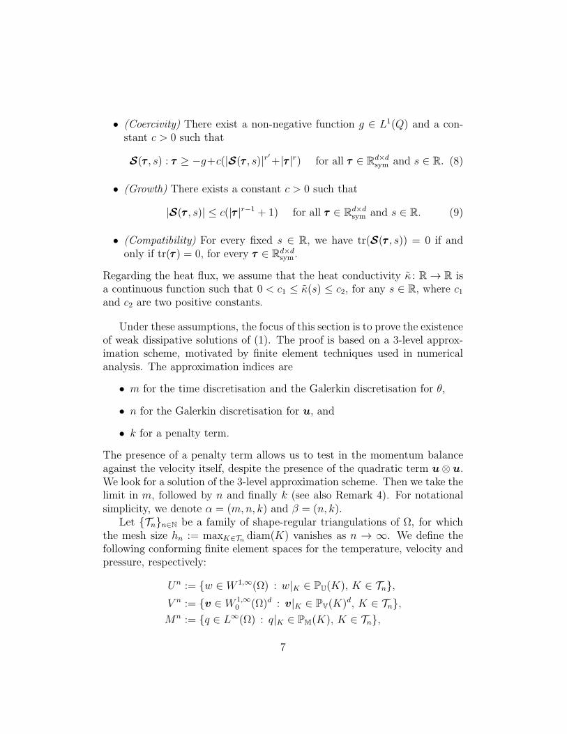
• (Coercivity) There exist a non-negative function g ∈ L1(Q) and a con-stant c > 0 such that
S(τττ , s) : τττ ≥ −g+c(|S(τττ , s)|r′
+|τττ |r) for all τττ ∈ Rd×dsym and s ∈ R. (8)
• (Growth) There exists a constant c > 0 such that
|S(τττ , s)| ≤ c(|τττ |r−1 + 1) for all τττ ∈ Rd×dsym and s ∈ R. (9)
• (Compatibility) For every fixed s ∈ R, we have tr(S(τττ , s)) = 0 if andonly if tr(τττ ) = 0, for every τττ ∈ R
d×dsym.
Regarding the heat flux, we assume that the heat conductivity κ : R → R isa continuous function such that 0 < c1 ≤ κ(s) ≤ c2, for any s ∈ R, where c1and c2 are two positive constants.
Under these assumptions, the focus of this section is to prove the existenceof weak dissipative solutions of (1). The proof is based on a 3-level approx-imation scheme, motivated by finite element techniques used in numericalanalysis. The approximation indices are
• m for the time discretisation and the Galerkin discretisation for θ,
• n for the Galerkin discretisation for u, and
• k for a penalty term.
The presence of a penalty term allows us to test in the momentum balanceagainst the velocity itself, despite the presence of the quadratic term u⊗ u.We look for a solution of the 3-level approximation scheme. Then we take thelimit in m, followed by n and finally k (see also Remark 4). For notationalsimplicity, we denote α = (m,n, k) and β = (n, k).
Let Tnn∈N be a family of shape-regular triangulations of Ω, for whichthe mesh size hn := maxK∈Tn diam(K) vanishes as n → ∞. We define thefollowing conforming finite element spaces for the temperature, velocity andpressure, respectively:
Un := w ∈ W 1,∞(Ω) : w|K ∈ PU(K), K ∈ Tn,
V n := v ∈ W 1,∞0 (Ω)d : v|K ∈ PV(K)d, K ∈ Tn,
Mn := q ∈ L∞(Ω) : q|K ∈ PM(K), K ∈ Tn,
7

where PU(K), PV(K), and PM(K) denote spaces of polynomials on the ele-ment K ∈ Tn. These must be chosen in such a way that certain stabilityproperties are satisfied (see Assumption 2 below). We also introduce thefollowing useful subspace of discretely divergence free functions of V n:
V ndiv :=
v ∈ V n :
∫
Ω
q div v = 0 for all q ∈Mn
.
Although the formulation (6) does not include the pressure, in practice theincompressibility constraint is enforced at the discrete level by means of aLagrange multiplier, which could be interpreted as a discrete pressure. Forthis reason, we also introduce appropriate assumptions on the pressure spacein what follows.
Assumption 2. The finite element spaces Un, V n, and Mn satisfy the fol-lowing properties.
• (Approximability) For an arbitrary s ∈ [1,∞), one has that
infw∈Un
‖w − w‖W 1,s(Ω) → 0 as n→ ∞ ∀w ∈ W 1,s(Ω),
infv∈V n
‖v − v‖W 1,s(Ω) → 0 as n→ ∞ ∀v ∈ W 1,s(Ω)d,
infq∈Mn
‖q − q‖Ls(Ω) → 0 as n→ ∞ ∀ q ∈ Ls(Ω).
• (Fortin Projector ΠnV ) For every n ∈ N, there exists Πn
V : W 1,10 (Ω)d →
V n, a linear projector, that satisfies the usual stability and divergencepreservation properties. That is, for any v ∈ W 1,1
0 (Ω)d, we have
∫
Ω
q div v =
∫
Ω
q div(ΠnV v) ∀ q ∈Mn,
and
‖ΠnV v‖W 1,s(Ω) ≤ c‖v‖W 1,s(Ω),
where s ∈ [1,∞) is arbitrary and c > 0 is a constant that is independentof n.
8

• (Projectors ΠnU , Πn
M) For every n ∈ N, we assume that there existΠn
U : W1,1(Ω) → Un and Πn
M : L1(Ω) →Mn, linear projectors, such that
‖ΠnUw‖W 1,s(Ω) ≤ c‖w‖W 1,s(Ω) ∀w ∈ W 1,s(Ω),
‖ΠnMq‖Ls(Ω) ≤ c‖q‖Ls(Ω) ∀ q ∈ Ls(Ω),
where s ∈ [1,∞) is arbitrary and c > 0 is a constant, independent of n.
In the discretisation scheme, we employ the skew-symmetric form of theconvective term. More precisely, the trilinear forms meant to represent theconvective terms in the momentum and temperature equations are defined,respectively, as
B(u, v,w) :=
−
∫
Ω
u⊗ v : ∇w dx if V ndiv ⊂W 1,1
0,div(Ω)d,
1
2
∫
Ω
u⊗w : ∇v − u⊗ v : ∇w dx otherwise,
and
C(u, θ, η) :=
−
∫
Ω
uθ · ∇η dx if V ndiv ⊂W 1,1
0,div(Ω)d,
1
2
∫
Ω
uη · ∇θ − uθ · ∇η dx otherwise.
The advantage of this choice is that we recover the skew-symmetry propertythat is valid for the original convective term at the continuous level. Indeed,we have B[u, v, v] = 0 and C[v, η, η] = 0 for any u, v ∈ V n
div and η ∈ Um,regardless of whether the discretely divergence free velocities are also point-wise divergence free or not. This is crucial to obtaining a priori estimates onthe sequence of approximate solutions.
For the time discretisation, we take a sequence of time steps τmm∈N
such that T/τm ∈ N and τm → 0 as m → ∞. For each time step τm, we
work on the equidistant grid tjT/τmj=0 where we define tj := tmj := jτm for
0 ≤ j ≤ T/τm.
Given a sequence of functions vjT/τmj=0 belonging to some Banach space
X , we define the piecewise constant interpolant v ∈ L∞(0, T ;X) by
v(t) := vj for t ∈ (tj−1, tj], j ∈ 1, . . . , T/τm. (10a)
9

The piecewise linear interpolant v ∈ C([0, T ];X) is defined by
v(t) :=t− tj−1
τmvj +
tj − t
τmvj−1 for t ∈ [tj−1, tj ], j ∈ 1, . . . , T/τm.
(10b)Additionally, we define the time averages of a given function g ∈ Lp(0, T ;X)by
gj(·) :=1
τm
∫ tj
tj−1
g(t, ·) dt. (10c)
It is possible to then prove that the piecewise constant interpolant gm definedby (10a) for the sequence (gj)
T/τmj=0 satisfies ‖gm‖Lp(0,T ;X) ≤ ‖g‖Lp(0,T ;X) and
gm → g strongly in Lp(0, T ;X) as m→ ∞ [26].The formulation of the discrete problem with parameters α = (m,n, k)
and corresponding existence result is as follows.
Proposition 1. Let r > 2dd+2
and let α = (m,n, k) be fixed approximation
parameters. Suppose that the data f ∈ Lr′(0, T ;W−1,r′(Ω)d), u0 ∈ L2div(Ω)
d
and θ0 ∈ L1(Ω) are given, such that θ0 ≥ c∗ > 0 for a constant c∗. We definethe initialisations
uα0 = P n
Vu0, θα0 = PmU θ
n0 ,
where P nV , P
mU are the L2-projection operators onto V n
div, Um, respectively,
and θn0 is defined as follows. We extend θ0 by c∗ outside of Ω and define θn0 =ρ 1
n∗ θ0, where ρ 1
nis a mollification kernel of radius 1
n. Let fm
j ∈ W−1,r′(Ω)d
be the sequence of time averages associated to f . Define r⊛ to be an arbitrarybut fixed number that is greater than max2r′, 5.
For every j ∈ 1, . . . , m, defining solutions recursively, there exist uαj ∈
V ndiv and θαj ∈ Um such that∫
Ω
δuαj ·v+
∫
Ω
S(DDDuαj , θ
αj ) : DDDv+
1
k
∫
Ω
|uαj |
r⊛−2uαj ·v+B[uα
j ,uαj , v] = 〈fm
j , v〉,
(11)and∫
Ω
δθαj ψ +
∫
Ω
κ(θαj )∇θαj · ∇ψ + C[uα
j , θαj , ψ] =
∫
Ω
DDDuαj : S(DDDuα
j , θαj )ψ, (12)
for every v ∈ V ndiv and ψ ∈ Um. Here δ denotes the backwards difference
quotient of order 1, namely,
δuαj :=
uαj − uα
j−1
τm, δθαj :=
θαj − θαj−1
τ.
10

Proof. The proof makes use of the following corollary to Brouwer’s fixedpoint theorem [27, Cor. 1.1]. The problem of finding a z ∈ X such thatF (z) = 0 where F : X → X is a function defined on a finite dimensionalHilbert space X has a solution z∗ if there exists a λ > 0 such that 〈F (z), z〉 >0 for every z ∈ X with ‖z‖ = λ. Furthermore, the solution satisfies ‖z∗‖ ≤ λ.
Suppose uαj−1 ∈ V n
div is given, for a j ∈ 1, . . . , T/τm. For fixed (u, θ) ∈V ndiv × Um, consider the problem of finding u ∈ V n
div such that F1(u) = 0where F1 is defined by
〈F1(u), v〉 :=
∫
Ω
u− uαj−1
τm· v + S(DDDu, θ) : DDDv +
1
k|u|r
⊛−2u · v
+ B[u,u, v]− 〈fmj , v〉,
(13)
for v ∈ V ndiv. Testing in (13) with v = u and using the fact that S(DDD(u), θ) :
DDD(u) ≥ 0 alongside the skew-symmetry of B, we find that
〈F1(u),u〉 ≥1
τm‖u‖2L2(Ω) −
∫
Ω
1
τmuα
j−1 · u dx− 〈fmj ,u〉
≥1
τm‖u‖2L2(Ω) − ε(‖u‖2L2(Ω) + ‖u‖2W 1,r(Ω))
− C(ε)
(
1
τ 2m‖uα
j−1‖2L2(Ω) + ‖fm
j ‖2W−1,r′(Ω)
)
,
where in the last step we use Young’s inequality. Choosing ε sufficientlysmall and using the equivalence of norms in finite dimensional spaces, theaforementioned corollary to Brouwer’s fixed point theorem guarantees thatthe solution operator H1 : V
ndiv × Um → V n
div given by H1(u, θ) := u is welldefined. Furthermore, the solution satisfies ‖u‖W 1,r(Ω) ≤ K1 where K1 =
K1(m,n) > 0 is independent of u and θ.Similarly, we define H2 : V
ndiv × Um → Um to be the solution operator
associated to the function
〈F2(θ), ψ〉 :=
∫
Ω
θ − θαj−1
τmψ+
∫
Ω
κ(θ)∇θ ·∇ψ+C[u, θ, ψ]−
∫
Ω
DDDu : S(DDDu, θ)ψ.
(14)Indeed, we set θ := H2(u, θ) if a solution θ exists to F2(θ) = 0. Using asimilar reasoning as above, we see that, if ‖u‖W 1,r(Ω) ≤ K1, the solution θexists and satisfies ‖θ‖H1(Ω) ≤ K2 where K2 > 0 depends on K1, m, and n,
but is independent of θ.
11

We observe that a fixed point of the operator H : V ndiv ×Um → V n
div ×Um
defined by H(u, θ) := (H1(u, θ), H2(u, θ)) is precisely a solution of (11) and(12). By the arguments above, we see that the operator H maps BV
K1×BU
K2
back into itself, where BVK1
⊂ V ndiv and BU
K2⊂ Um are the balls of radii
K1 and K2, respectively. Thus, if we can verify the continuity of H1 andH2, Brouwer’s fixed point theorem guarantees the existence of a solution,completing the proof of the proposition.
Let us examine H2 first. We take arbitrary (u, θ), (w, η) ∈ BVK1
×BUK2
andsubtract the equations for H2(u, θ) and H2(w, η). Testing in the resultingequation against the difference ψ = H2(u, θ)−H2(w, η) yields (recalling thatthe heat flux is monotone)
1
τm‖H2(u, θ)−H2(w, η)‖
2L2(Ω)
≤ C[w, H2(w, η), H2(u, θ)−H2(w, η)]− C[u, H2(u, θ), H2(u, θ)−H2(w, η)]
+
∫
Ω
(S(DDDu, θ) : DDDu− S(DDDw, η) : DDDw)(H2(u, θ)−H2(w, η)) dx
≤ C[u−w, H2(u, θ), H2(w, η)]
+
∫
Ω
(S(DDDu, θ) : DDDu− S(DDDw, η) : DDDw)(H2(u, θ)−H2(w, η)) dx
≤ cn‖u−w‖W 1,r(Ω)‖H2(u, θ)‖H1(Ω)‖H2(w, η)‖H1(Ω)
+ ‖S(DDDu, θ) : DDDu− S(DDDw, η) : DDDw‖L2(Ω)‖H2(u, θ)−H2(w, η)‖L2(Ω),
which, recalling the boundedness of H2, implies that H2(u, θ) → H2(w, η) as(u, θ) → (w, η). In the above, we note that we rely heavily on the equivalenceof norms in finite dimensional spaces. In a similar fashion but reasoning forH1, we have that
1
τm‖H1(u, θ)−H1(w, η)‖
2L2(Ω)
≤ B[u−w, H1(u, θ), H1(w, η)]
+
∫
Ω
(S(DDDH1(w, η), η)− S(DDDH1(u, θ), θ)) : (DDDH1(u, θ)−DDDH1(w, η)) dx
≤ B[u−w, H1(u, θ), H1(w, η)]
+
∫
Ω
(S(DDDH1(u, θ), η)− S(DDDH1(u, θ), θ)) : (DDDH1(u, θ)−DDDH1(w, η)) dx,
12

where in the first inequality we use that the operator u 7→ 1k|u|r
⊛−2u ismonotone, since it is the derivative of a convex function. In the second in-equality, we employ the monotonicity of S. Reasoning as above, this impliesthat H1 is continuous, concluding the proof of the assertion.
The first step towards obtaining a dissipative solution of the originalproblem is to take the limit in the discretisation parameter m while keepingβ = (n, k) fixed.
Lemma 2. Let the assumptions of Proposition 1 hold and let (uαj , θ
αj )
mj=1
be the sequence of solutions constructed there. There exist a constant C1,independent of α, and a constant C2 = C2(n), independent of k and m, suchthat
‖uα‖2L∞(0,T ;L2(Ω)) + τm‖∂tuα‖2L2(Q) + ‖uα‖rLr(0,T ;W 1,r(Ω))
+1
k‖uα‖r
⊛
Lr⊛(Q)+ ‖S(DDDuα, θ
α)‖r
′
Lr′(Q)≤ C1,
and
‖θα‖L∞(0,T ;L2(Ω)) + τm‖∂tθ
α‖2L2(Q) + ‖∇θα‖2L2(Q) ≤ C2.
Proof. Testing in (11) against uαj , we see that
1
2τm
(
‖uαj ‖
2L2(Ω) − ‖uα
j−1‖2L2(Ω) + ‖uα
j − uαj−1‖
2L2(Ω)
)
+
∫
Ω
S(DDDuαj , θ
αj ) : DDDu
αj
+1
k‖uα
j ‖r⊛
Lr⊛(Ω)= 〈fm
j ,uαj 〉 ≤ C(ε)‖fm
j ‖r′
W−1,r′(Ω)+ ε‖uα
j ‖rW 1,r(Ω),
where ε > 0 is to be fixed sufficiently small later. By the coercivity conditionsand making use of the Korn–Poincare inequality, we deduce that
‖uαj ‖
2L2(Ω) − ‖uα
j−1‖2L2(Ω) + τ 2m‖δu
αj ‖
2L2(Ω) + τm‖u
αj ‖
rW 1,r(Ω)
+ τm‖S(DDDuαj , θ
αj )‖
r′
Lr′(Ω)+τmk‖uα
j ‖r⊛
Lr⊛(Ω)
≤ C(r, ε)‖fm‖r
′
Lr′(tj−1,tj ;W−1,r′(Ω))+ c‖g‖L1(Qj
j−1)+ ετm‖u
αj ‖
rW 1,r(Ω),
(15)
where the function g comes from the coercivity assumption on S and Qjj−1 =
(tj−1, tj) × Ω for 1 ≤ j ≤ T/τm. Choosing ε sufficiently small, we absorbthe final term on the right-hand side into the left-hand side. Summing (15)
13

over the indices j = 1, . . . , l for an l ∈ 1, . . . , T/τm and maximising theresulting left-hand side, it follows that
τm
T/τm∑
j=1
[
τm‖δuαj ‖
2L2(Ω) + ‖uα
j ‖rW 1,r(Ω) + ‖S(DDDuα
j , θαj )‖
r′
Lr′(Ω)
]
+ max1≤j≤T/τm
‖uαj ‖
2L2(Ω) +
τmk
T/τm∑
j=1
‖uαj ‖
r⊛
Lr⊛(Ω)
≤ C(‖f‖r′
Lr′(0,T ;W−1,r′(Ω))+ ‖g‖L1(Q) + ‖u0‖
2L2(Ω)),
using the stability property
‖P nVu0‖L2(Ω) ≤ ‖u0‖L2(Ω). (16)
Similarly, testing in (12) against θαj yields
1
2τm
(
‖θαj ‖2L2(Ω) − ‖θαj−1‖
2L2(Ω) + ‖θαj − θαj−1‖
2L2(Ω)
)
+
∫
Ω
κ(θαj )|∇θαj |
2 dx
=
∫
Ω
S(DDDuαj , θ
αj ) : DDDu
αj θ
αj dx
≤ C
∫
Ω
(|DDDuαj |
r−1 + 1)|DDDuαj |θ
αj dx,
where we use Assumption 1 concerning the growth of S. However, using thefact that norms on finite-dimensional spaces are equivalent, we see that∫
Ω
(|DDDuαj |
r−1 + 1)|DDDuαj |θ
αj dx ≤ C
(
‖DDDuαj ‖
rL2r(Ω) + ‖DDDuα
j ‖L2(Ω)
)
‖θαj ‖L2(Ω)
≤ C(n)(
‖uαj ‖
rL2(Ω) + ‖uα
j ‖L2(Ω)
)
‖θαj ‖L2(Ω).
However, from the above, we know for instance that
max1≤j≤T/τm
‖uαj ‖
rL2(Ω) ≤ C
r21 ,
where C1 is the constant from the first bound and is independent of α. Itfollows that
1
2τm
(
‖θαj ‖2L2(Ω) − ‖θαj−1‖
2L2(Ω) + ‖θαj − θαj−1‖
2L2(Ω)
)
14

+
∫
Ω
κ(θαj )|∇θαj |
2 ≤ C(n)‖θαj ‖L2(Ω).
Hence, for an arbitrary l ∈ 1, . . . , T/τm, we have
‖θαl ‖2L2(Ω) + τm
l∑
j=1
[
τm‖δθαj ‖
2L2(Ω) + ‖∇θαj ‖
2L2(Ω)
]
≤ C(n)τm
l∑
j=1
‖θαj ‖L2(Ω) + ‖θα0 ‖2L2(Ω)
≤ C(n)
(
τm
l∑
j=1
‖θαj ‖2L2(Ω) + 1
)
.
The result follows by a discrete version of Gronwall’s inequality and thenrecalling the definition of the piecewise constant and piecewise linear inter-polants.
Using the a priori bounds of Lemma 2, standard weak compactness resultsand Simon’s lemma, the following convergence results are immediate (cf.[28]).
Corollary 3. There exists a limiting triple (uβ, θβ, SSSβ) such that the follow-
ing convergence results hold, up to a subsequence in m that we do not relabel:
uα ∗ uβ weakly-* in L∞(0, T ;L2(Ω)d);
uα uβ weakly in Lr(0, T ;W 1,r(Ω)d);
1
k|uα|r
⊛−2uα 1
k|uβ|r
⊛−2uβ weakly in L(r⊛)′(Q)d;
S(DDDuα, θα) SSS
βweakly in Lr′(Q)d×d;
θα ∗ θβ weakly-* in L∞(0, T ;L2(Ω));
θα θβ weakly in L2(0, T ;W 1,2(Ω)).
Furthermore, we have the following strong convergence results:
θα→ θβ strongly in L2(Q);
uα → uβ strongly in L2(Q)d.
15

Passing to the limit in the time discrete formulation, we see that thecouple (uβ, θβ) is a solution of the following semi-discrete problem. For everyφ ∈ C∞
0 ([0, T )), we have the momentum balance
−
∫
Q
uβ ·(
v∂tφ)
−
∫
Ω
P nVu0 ·
(
vφ(0))
+1
k
∫
Q
|uβ|r⊛−2uβ · (vφ)
+
∫ T
0
B[uβ,uβ, v]φ+
∫
Q
SSSβ: DDD(vφ) =
∫ T
0
〈f , v〉φ,
(17)
for every v ∈ V ndiv, and the temperature balance
−
∫
Q
θβψ∂tφ dx dt−
∫
Ω
θn0ψφ dx+
∫
Q
κ(θβ)∇θβ · ∇(
ψφ)
dx dt
+
∫ T
0
C[uβ, θβ, ψ]φ dt =
∫
Q
SSSβ: DDD(uβ)ψφ dx dt,
(18)
for every ψ ∈ W 1,∞(Ω). Furthermore, as a result of the strong convergence,
we can identify SSSβ= S(DDDuβ, θβ) a.e. in Q. Hence the triple (uβ, θβ, SSS
β)
is a solution of a suitable approximation of the original problem (1). Nowwe search for appropriate a priori bounds that allow us to take the limit asn→ ∞.
Lemma 4. Let (uβ, θβ, SSSβ) be the solution triple constructed in Corollary 3.
There exists a positive constant C1, independent of β, such that
‖uβ‖2L∞(0,T ;L2(Ω))+‖uβ‖rLr(0,T ;W 1,r(Ω))+1
k‖uβ‖r
⊛
Lr⊛(Q)+‖SSS
β‖r
′
Lr′(Q)≤ C1. (19)
Furthermore, there exists a positive constant C2, independent of β, such that
‖uβ‖L
r(d+2)d (Q)
≤ C2. (20)
Proof. The first bound (19) follows immediately from Lemma 2 and theweak lower semi-continuity of norms. The estimate (20) is a standard parabolicembedding, which is a consequence of the Gagliardo–Nirenberg inequality(see, for example, [26, Lm. 7.8]).
Lemma 5. Let (uβ, θβ, SSSβ) be the solution triple constructed in Corollary 3.
There exists a constant c∗ > 0, independent of β, such that
θβ ≥ c∗ > 0 a.e. in Q. (21)
16

There exists a constant C3 > 0, independent of β, such that
‖θβ‖L∞(0,T ;L1(Ω)) + ‖θβ‖Ls(Q) + ‖θβ‖Lq(0,T ;W 1,q(Ω)) ≤ C3, (22)
for s ∈ [1, 53) and q ∈ [1, 5
4). Moreover, for sufficiently large p, there exists a
positive constant C4 = C4(k), independent of n, such that
‖∂tθβ‖L1(0,T ;W−1,p′(Ω)) ≤ C4. (23)
Proof. For (21) and (22), we reason as in [9]. Although the authors therework in the setting r = 2, the argument is independent of r and so can beused here.
Consequently, we see from (18), (19), (20) and (22) that (23) must alsohold. We note that the exponent r⊛ in the penalty term was chosen to ensurethat the term uβ · ∇θβ , which appears in the modified convective term C,belongs to L1+δ(Q), for some δ > 0.
Similarly as in Corollary 3, the estimates above ensure that there exists
a limiting triple (uk, θk, SSSk) such that the following convergences hold, up to
a subsequence that we do not relabel:
uβ ∗ uk weakly-* in L∞(0, T ;L2(Ω)d);
uβ uk weakly in Lr(0, T ;W 1,r(Ω)d);
1
k|uβ|r
⊛−2uβ 1
k|uk|r
⊛−2uk weakly in L(r⊛)′(Q)d;
uβ → uk strongly in Lq1(Q)d, q1 ∈[
1, r⊛)
;
Sk(DDDuβ, θβ) SSS
kweakly in Lr′(Q)d×d;
θβ θk weakly-* in Lq2(0, T ;W 1,q2(Ω)), q2 ∈[
1,5
4
)
;
θβ → θk strongly in Lq3(Q), q3 ∈[
1,5
3
)
.
These convergence results are sufficient to allow passage to the limit in themomentum equation. Thus we obtain
∫
Ω
∂tuk·v+
∫
Ω
SSSk: DDDv−
∫
Ω
(uk⊗uk) : DDDv+1
k
∫
Ω
|uk|r⊛−2uk·v = 〈f , v〉, (24)
17

for every v ∈ C∞0,div(Ω)
d and a.e. t ∈ (0, T ). The convective term can be
now written in its original form since divuk = 0 pointwise. Furthermore, we
claim that SSSk= S(DDDuk, θk) a.e. in Q. Indeed, since k is fixed, the velocity uk
is an admissible test function in (24). Therefore we have an energy identityavailable (cf. [29, Eq. 4.103]). This makes it straightforward to prove that
lim supn→∞
∫
Q
S(DDDuβ, θβ) : DDDuβ dx dt ≤
∫
Q
SSSk: DDDuk dx dt. (25)
Recalling the growth condition (9), we observe that the dominated conver-gence theorem implies that, for an arbitrary τττ ∈ Lr(Q)d×d, we have
S(τττ , θβ) → S(τττ , θk) strongly in Lr′(Ω)d×d, (26)
as n → ∞. Combining the monotonicity property (7) of S with (25) and(26) yields, for an arbitrary τττ ∈ Lr(Q)d×d,
0 ≤ lim supn→∞
∫
Q
(S(DDDuβ, θβ)− S(τττ , θβ)) : (DDDuβ − τττ ) dx dt
≤
∫
Q
(SSSk− S(τττ , θk)) : (DDDuk − τττ) dx dt.
Choosing τττ = DDDuk ± εσσσ for an arbitrary σσσ ∈ C∞0 (Q)d×d and letting ε → 0
concludes the proof of the claim.In order to pass to the limit in the temperature equation, we need to
investigate the convergence of S(DDDuβ, θβ) : DDDuβ in L1(Q). Firstly, from themonotonicity of S, we see that
∫
Q
SSSk: DDDuk dx dt ≤ lim inf
n→∞
∫
Q
S(DDDuβ, θβ) : DDDuβ dx dt,
and so, by (25), the equality actually holds. In turn, this implies that
(S(DDDuβ, θβ)− S(DDDuk, θk)) : (DDDuβ −DDDuk) → 0 strongly in L1(Q),
noting that the sequence on the left-hand side is non-negative. Writing
S(DDDuβ, θβ) : DDDuβ = S(DDDuβ, θβ) : DDDuk + S(DDDuk, θk) : (DDDuβ −DDDuk)
+ (S(DDDuβ, θβ)− S(DDDuk, θk)) : (DDDuβ −DDDuk),
18

immediately yields that S(DDDuβ, θβ) : DDDuβ S(DDDuk, θk) : DDDuk weakly inL1(Q) as n → ∞. Hence, the limiting functions satisfy the temperaturebalance∫
Ω
∂tθkψ +
∫
Ω
κ(θk)∇θk · ∇ψ −
∫
Ω
ukθk · ∇ψ =
∫
Ω
S(DDDuk, θk) : DDDukψ (27)
for every ψ ∈ W 1,∞(Ω) and a.e. t ∈ (0, T ).Using the weak lower semi-continuity of norms, we obtain the following
estimates:
‖uk‖L∞(0,T ;L2(Ω)) + ‖uk‖Lr(0,T ;W 1,r(Ω)) +1
k‖uk‖r
⊛
Lr⊛(Q)+ ‖S(DDDuk, θk)‖Lr′(Q)
+ ‖uk‖L
r(d+2)d (Q)
+ ‖θk‖L∞(0,T ;L1(Ω)) + ‖θk‖Ls(Q) + ‖θk‖Lq(0,T ;W 1,q(Ω)) ≤ C1,
(28)
for arbitrary s ∈ [1, 53) and q ∈ [1, 5
4), and a constant C1 that is independent
of k. It follows that, up to a subsequence in k that we do not relabel, thefollowing convergence results hold:
uk ∗ u weakly-* in L∞(0, T ;L2(Ω)d);
uk u weakly in Lr(0, T ;W 1,r(Ω)d);
uk → u strongly in Lq1(Q)d, q1 ∈[
1,r(d+ 2)
d
)
;
uk(s, ·) → u(s, ·) strongly in L2(Ω)d, for a.e. s ∈ (0, T );
1
k|uk|r
⊛−2uk → 0 strongly in L1(Q)d;
Sk(DDDuk, θk) SSS weakly in Lr′(Q)d×d;
θk∗ θ weakly-* in Ls(0, T ;W 1,q2(Ω)), q2 ∈
[
1,5
4
)
;
θk → θ strongly in Lq3(Q), q3 ∈[
1,5
3
)
;
θk(s, ·) → θ(s, ·) strongly in L1(Ω), for a.e. s ∈ (0, T ).
The above convergences do not suffice to pass to the limit in the temperatureequation. Hence, at this stage we turn to the entropy balance. The followinglemma states the a priori estimates that are satisfied by the entropy, whichwe use when passing to the limit in k.
19

Lemma 6. Let the assumptions of Proposition 1 hold and let (uk, θk, SSSk) be
the limiting solution of (24), (27) that is constructed by taking the limit asm → ∞, then n → ∞ for the solution triple from Proposition 1. Definethe entropy by Sk = log θk (without loss of generality we set cv ≡ 1). Thereexists a constant C5, independent of k, such that
‖Sk‖L2(0,T ;W 1,2(Ω)) + ‖Sk‖L∞(0,T ;Lq(Ω)) ≤ C5, (29)
for arbitrary q ∈ [1,∞).
Proof. We notice that, for any λ ∈ (−1, 0), the function f(x) = log2 xxλ+1 is
bounded on [1,∞). Assuming that θk ≥ 1, it follows that log2 θk ≤ cθkλ+1
fora constant c > 0. On the other hand, now suppose that c∗ < 1 and considerwhen θk ∈ [c∗, 1). We notice that log2 θk ≤ log2 c∗ and so we can bound
log2 θk
θkλ+1 ≤log2 c∗
cλ+1∗
<∞.
Consequently log2 θk ≤ cθkλ+1
a.e. in Q for some positive constant c that isindependent of k. Furthermore, from the inequality 0 < c∗ ≤ θk, we havethat θk
−2≤ c−1−λ
∗ θkλ−1
. Hence, we deduce that
‖Sk‖L2(0,T ;W 1,2(Ω)) = ‖ log θk‖L2(0,T ;W 1,2(Ω)) ≤ c‖θk1+λ2 ‖L2(0,T ;W 1,2(Ω)) ≤ c.
Using a similar argument but with logq θθ
, we deduce the latter bound in thestatement of the lemma as required.
As a consequence of Lemma 6 we obtain that, up to a subsequence in kthat we do not relabel, we have the convergences
Sk S weakly in L2(0, T ;W 1,2(Ω)),
Sk ∗ S weakly in L∞(0, T ;Lq5(Ω)), q5 ∈ [1,∞).
Additionally, the almost everywhere convergence of θk in Q allows us toidentify S = log θ. We now focus on proving that the limiting functionsconstitute a dissipative weak solution of (1) in the sense of Definition 1.
Theorem 7. Let the assumptions of Proposition 1 hold. Then, the quartet(u, θ,SSS, S) constructed above is a dissipative weak solution of (1) in the senseof Definition 1.
20

Proof. The estimates in (28) and the convergences they induce make itstraightforward to pass to the limit in the momentum equation and deducethat the couple (u,SSS) satisfies (6b).
The constitutive relation (6a) can be identified in the same manner asbefore, assuming that we can prove an estimate that is analogous to (25).Since the velocity u is not an admissible test function in the balance ofmomentum, there is no energy identity available. Hence obtaining such anestimate is not straightforward. Thankfully, this difficulty can be dealt withby testing with a Lipschitz truncation of the error uk − u. In doing so, it ispossible to prove the existence of a nonincreasing sequence of sets Ej ⊂ Qsuch that |Ej | → 0 as j → ∞ and
lim supk→∞
∫
Q\Ej
S(DDDuk, θk) : DDDuk dx dt =
∫
Q\Ej
SSS : DDDu dx dt for any j ∈ N.
(30)The details of this argument can be found, for example, in [30, Thm. 3.3].This implies that SSS = S(DDDu, θ) a.e. in Q \ Ej and that SSSk : DDDuk SSS : DDDuweakly in L1(Q \ Ej) for any j ∈ N. The measure of the sets Ej vanishes asj → ∞ and so identification of the constitutive relation (6a) follows.
Next, we turn to the entropy balance. Testing the temperature equation(27) with ψ/θk, where ψ ∈ C∞
0 ([0, T );C1(Ω)) is an arbitrary function suchthat ψ ≥ 0, we obtain the following equation for the entropy Sk:
−
∫
Q
Sk∂tψ dx−
∫
Ω
ψ(0) log θ0 −
∫
Q
Skuk · ∇ψ +
∫
Q
κ(θk)∇θk
θk· ∇ψ
=
∫
Q
κ(θk)|∇θk|2
θk2ψ +
∫
Q
S(DDDuk, θk) : DDD(uk)
θkψ ≥ 0,
(31)
for every ψ ∈ C∞0 ([0, T );C1(Ω)) such that ψ ≥ 0. Now, cf. [12], we claim
that
lim infk→∞
∫
Q
SSSk : DDDukη dx dt ≥
∫
Q
SSS : DDDuη dx dt, (32)
for any non-negative function η ∈ L∞(Q). Since S(DDDu, θ) : DDDuη is integrable,for every ε > 0 there exists a δ > 0 such that, for any E ⊂ Q with |E| ≤ δ,we have
∫
Q
S(DDDu, θ) : DDDuη dx dt ≤ ε.
21

Noting that S(DDDuk, θk)η is non-negative and choosing j ∈ N sufficiently largeso that |Ej| ≤ δ for the sets Ej described in (30), we have
lim infk→∞
∫
Q
SSSk: DDDukη ≥ lim inf
k→∞
∫
Q\Ej
SSSk: DDDukη
=
∫
Q\Ej
SSS : DDDuη ≥
∫
Q
SSS : DDDuη − ε.
Combining this with the weak lower semi-continuity of the L2-norm alongsidethe convergence of the sequence (
√
ψκ(θk)∇Sk)k, we can take the limit in theequation (31) for Sk and obtain the entropy inequality (6c). The assumptionr > 2d
d+2guarantees the compactness of Skuk in the advective term.
Finally, we consider the balance of total energy. First, we note that, sincethe velocity uk is an admissible test function in (24), the following energyidentity holds for a.e. τ ∈ (0, T ) [29, Eq. 4.103]:
1
2‖uk(τ, ·)‖2L2(Ω) +
∫
Qτ
SSSk : DDDuk +
1
k‖uk‖r
⊛
Lr⊛(Qτ )=
∫ τ
0
〈f ,uk〉+1
2‖u0‖
2L2(Ω).
(33)Testing the balance of temperature with the approximate indicator functionψj of the interval (0, τ) and letting j → ∞, we add the result to (33) toobtain
[
∫
Ω
|uk(t, ·)|2
2+ θk(t, ·) dx
]t=τ
t=0+
1
k‖uk‖r
⊛
Lr⊛(Qτ )=
∫ τ
0
〈f ,uk〉 dt,
which, taking k → ∞, implies the balance of total energy (6d).
Remark 1. So far we have assumed that the constitutive relation is of thespecific form SSS = S(DDDu, θ), but the approach presented here can be almostidentically applied to models of the form DDDu = D(SSS, θ), which include forinstance Glen’s model for ice dynamics [31]. In fact, this is true also forimplicit models in which the constitutive relation is written as
GGG(·,SSS,DDDu) = 0 a.e. in Q, (34)
where GGG : Q×Rd×dsym×R
d×dsym → R
d×dsym is a function defining a maximal monotone
r-graph (see [30] for an in-depth discussion of these models). An important
22

example of a model that can be described in such manner is the Herschel–Bulkley model for viscoplastic flow:
|SSS| ≤ τ∗ ⇐⇒ DDDu = 0,
|SSS| > τ∗ ⇐⇒ SSS = K|DDDu|r−2DDDu+τ∗
|DDDu|DDDu,
(35)
where τ∗, K > 0 are parameters. We note that this model can also bedescribed using the implicit function
GGG(SSS,DDDu) := (|SSS| − τ∗)+SSS−K|DDDu|r−2(τ∗ + (|SSS| − τ∗)
+)DDDu. (36)
For the model with r = 2, the model with temperature dependent activationparameters can also be included (cf. [12]). When tackling the question ofexistence of dissipative weak solutions for implicit models one could employa finite element formulation including the stress SSS as an unknown, in ananalogous way to the formulations analysed in [32, 28].
Remark 2. As mentioned in the introduction, the approximation schemeintroduced in Proposition 1 is better suited to numerical analysis than theone proposed in [9], since we do not require the computation of a Helmholtzdecomposition nor a quasi-compressible approximation. The admissibilityproblem of the velocity is instead dealt with by means of a penalty term.
Remark 3. The arguments presented in this Section can be applied almostverbatim to the problem with Navier’s slip boundary conditions, in whichcase one obtains also the existence of an integrable pressure p ∈ L1(Q).Assuming that r > 3d
d+2, the results from [11] guarantee even that a weak
version of the energy balance (3) holds. The results from this paper thenconstitute an extension to the regime r ∈ ( 2d
d+2, 3dd+2
] for problems with suchboundary conditions.
Remark 4. The proof of Theorem 7 is based on a 3-level approximationscheme that in practice could be very likely simplified. The reason for con-sidering two discretisation indices m and n is to simplify the argument forobtaining the positivity of the temperature (21) and the estimates (22), sinceotherwise these properties would have to be obtained at the finite elementlevel. The index k associated to the penalty term can very likely also beavoided, but a discrete version of a parabolic Lipschitz truncation would beneeded, which although very plausible, is not available at the time of thispublication (a steady version was developed in [33]).
23
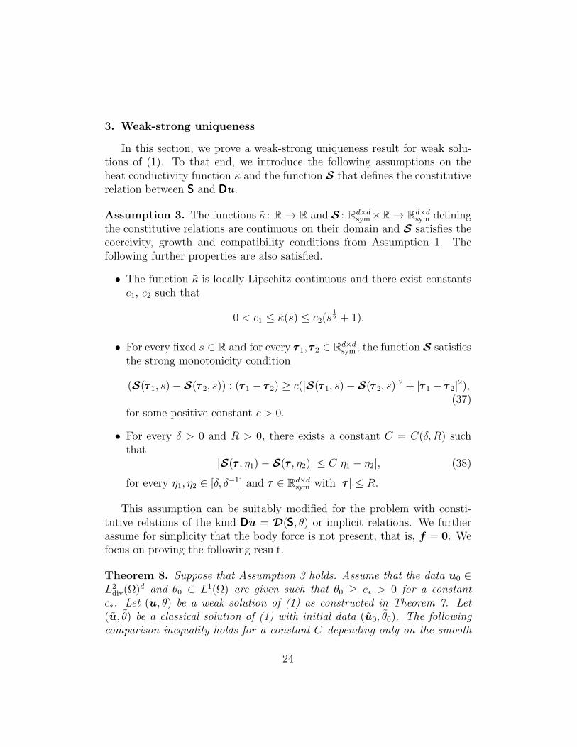
3. Weak-strong uniqueness
In this section, we prove a weak-strong uniqueness result for weak solu-tions of (1). To that end, we introduce the following assumptions on theheat conductivity function κ and the function S that defines the constitutiverelation between SSS and DDDu.
Assumption 3. The functions κ : R → R and S : Rd×dsym×R → R
d×dsym defining
the constitutive relations are continuous on their domain and S satisfies thecoercivity, growth and compatibility conditions from Assumption 1. Thefollowing further properties are also satisfied.
• The function κ is locally Lipschitz continuous and there exist constantsc1, c2 such that
0 < c1 ≤ κ(s) ≤ c2(s12 + 1).
• For every fixed s ∈ R and for every τττ 1, τττ 2 ∈ Rd×dsym , the function S satisfies
the strong monotonicity condition
(S(τττ 1, s)− S(τττ 2, s)) : (τττ 1 − τττ 2) ≥ c(|S(τττ 1, s)− S(τττ 2, s)|2 + |τττ 1 − τττ 2|
2),(37)
for some positive constant c > 0.
• For every δ > 0 and R > 0, there exists a constant C = C(δ, R) suchthat
|S(τττ , η1)− S(τττ , η2)| ≤ C|η1 − η2|, (38)
for every η1, η2 ∈ [δ, δ−1] and τττ ∈ Rd×dsym with |τττ | ≤ R.
This assumption can be suitably modified for the problem with consti-tutive relations of the kind DDDu = D(SSS, θ) or implicit relations. We furtherassume for simplicity that the body force is not present, that is, f = 0. Wefocus on proving the following result.
Theorem 8. Suppose that Assumption 3 holds. Assume that the data u0 ∈L2div(Ω)
d and θ0 ∈ L1(Ω) are given such that θ0 ≥ c∗ > 0 for a constantc∗. Let (u, θ) be a weak solution of (1) as constructed in Theorem 7. Let(u, θ) be a classical solution of (1) with initial data (u0, θ0). The followingcomparison inequality holds for a constant C depending only on the smooth
24
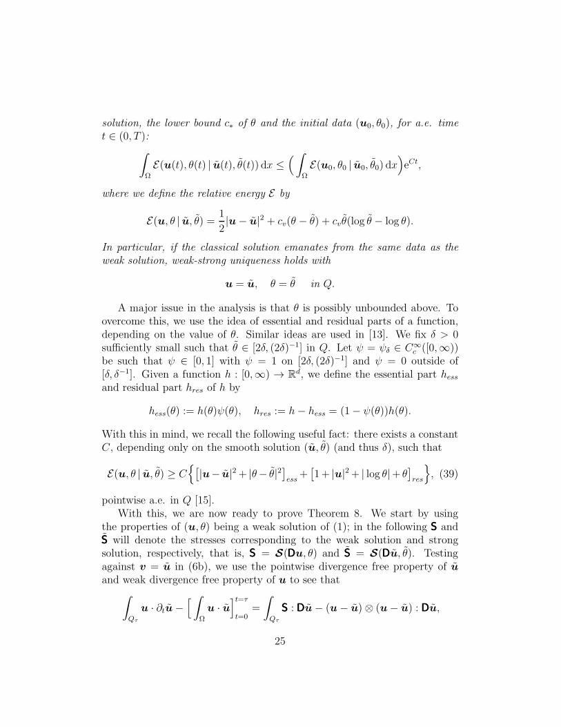
solution, the lower bound c∗ of θ and the initial data (u0, θ0), for a.e. timet ∈ (0, T ):
∫
Ω
E(u(t), θ(t) | u(t), θ(t)) dx ≤(
∫
Ω
E(u0, θ0 | u0, θ0) dx)
eCt,
where we define the relative energy E by
E(u, θ | u, θ) =1
2|u− u|2 + cv(θ − θ) + cvθ(log θ − log θ).
In particular, if the classical solution emanates from the same data as theweak solution, weak-strong uniqueness holds with
u = u, θ = θ in Q.
A major issue in the analysis is that θ is possibly unbounded above. Toovercome this, we use the idea of essential and residual parts of a function,depending on the value of θ. Similar ideas are used in [13]. We fix δ > 0sufficiently small such that θ ∈ [2δ, (2δ)−1] in Q. Let ψ = ψδ ∈ C∞
c ([0,∞))be such that ψ ∈ [0, 1] with ψ = 1 on [2δ, (2δ)−1] and ψ = 0 outside of[δ, δ−1]. Given a function h : [0,∞) → R
d, we define the essential part hessand residual part hres of h by
hess(θ) := h(θ)ψ(θ), hres := h− hess = (1− ψ(θ))h(θ).
With this in mind, we recall the following useful fact: there exists a constantC, depending only on the smooth solution (u, θ) (and thus δ), such that
E(u, θ | u, θ) ≥ C
[
|u− u|2+ |θ− θ|2]
ess+[
1+ |u|2+ | log θ|+ θ]
res
, (39)
pointwise a.e. in Q [15].With this, we are now ready to prove Theorem 8. We start by using
the properties of (u, θ) being a weak solution of (1); in the following SSS andSSS will denote the stresses corresponding to the weak solution and strongsolution, respectively, that is, SSS = S(DDDu, θ) and SSS = S(DDDu, θ). Testingagainst v = u in (6b), we use the pointwise divergence free property of uand weak divergence free property of u to see that
∫
Qτ
u · ∂tu−[
∫
Ω
u · u]t=τ
t=0=
∫
Qτ
SSS : DDDu− (u− u)⊗ (u− u) : DDDu,
25

where we denote Qτ = (0, τ)× Ω. It follows that
[
∫
Ω
|u− u|2
2dx]t=τ
t=0=[
∫
Ω
|u|2
2dx]t=τ
t=0+
∫
Qτ
u · ∂tu dx dt−[
∫
Ω
u · udx]t=τ
t=0
=[
∫
Ω
|u|2
2dx]t=τ
t=0−
∫
Qτ
(u− u) · ∂tudx dt
+
∫
Qτ
SSS : DDDu− (u− u)⊗ (u− u) : DDDu dx dt.
Using the total energy balance for the weak solution, we replace the firstterm on the right-hand side to deduce that
[
∫
Ω
|u− u|2
2+ cvθ dx
]t=τ
t=0−
∫
Qτ
SSS : DDDudx dt
≤ −
∫
Qτ
(u− u) · ∂tu+ (u− u)⊗ (u− u) : DDDu dx dt.
(40)
Using the fact that (u, θ) is a classical solution and, in particular, satisfies(1b) pointwise, we rewrite the first term on the right-hand side of (40) as
∫
Qτ
(u− u) · ∂tu dx dt =
∫
Qτ
(u− u) · div(SSS− u⊗ u) dx dt. (41)
Applying the appropriate divergence-free properties of u and u, it followsthat
∫
Qτ
(u− u) · div(u⊗ u) dx dt
=
∫
Qτ
(u− u) · u div(u) + (u− u)⊗ u : ∇u dx dt
=1
2
∫
Qτ
(u− u) : ∇(|u|2) dx dt
= 0.
(42)
Substituting (41) and (42) into (40) yields
[
∫
Ω
|u− u|2
2+ cvθ dx
]t=τ
t=0+
∫
Qτ
−SSS : DDDu− SSS : DDDu+ SSS : DDDu dx dt
≤ −
∫
Qτ
(u− u)⊗ (u− u) : DDDu dx dt.
(43)
26

Next, we need to use of the entropy inequality for the weak solution andentropy balance for the classical solution. Testing in the entropy inequality(6c) against θ and using the idenitifcation S = cv log θ, we obtain
[
∫
Ω
cvθ log θ dx]t=τ
t=0−
∫
Qτ
cv log θ∂tθ + cv log θu · ∇θ + q · ∇θ dx dt
≥
∫
Qτ
θq ·∇θ
θdx dt +
∫
Qτ
SSS : DDDu
θθ dx dt.
Adding this to (43), we get
[
∫
Ω
|u− u|2
2+ cvθ − cvθ log θ dx
]t=τ
t=0+
∫
Qτ
−θ
θq ·
∇θ
θ+θ
θq ·
∇θ
θdx dt
+
∫
Qτ
θ
θSSS : DDDu− SSS : DDDu+ SSS : DDDu+ SSS : DDDu dx dt
≤ −
∫
Qτ
(u− u)⊗ (u− u) : DDDu+ cv log θ∂tθ + cv log θu · ∇θ dx dt.
(44)We want to add terms to the left-hand side of (44) in order to have a terminvolving the relative energy. Recalling the definition of the relative energyE(u, θ | u, θ), we consider
[
∫
Ω
−cvθ + cvθ log θ dx]t=τ
t=0=
∫
Qτ
cv∂tθ log θ dx dt.
Adding this into (44), we deduce that
[
∫
Ω
E(u, θ | u, θ)]t=τ
t=0+
∫
Qτ
θ
θSSS : DDDu− SSS : DDDu− SSS : DDDu+ SSS : DDDu
−
∫
Qτ
θ
θq ·
∇θ
θ−θ
θq ·
∇θ
θ
≤ −
∫
Qτ
(u− u)⊗ (u− u) : DDDu+ cv log θ∂tθ + cv log θu · ∇θ − cv∂tθ log θ.
(45)Using the energy balance (1a) for the classical solution, multiplying by log θ−log θ and integrating over Qτ , we see that the second and fourth terms onthe right-hand side of (45) can be rewritten as∫
Qτ
cv∂tθ(
log θ− log θ)
=
∫
Qτ
cv(
log θ− log θ)[
SSS : DDDu− div(θu+ q)]
. (46)
27
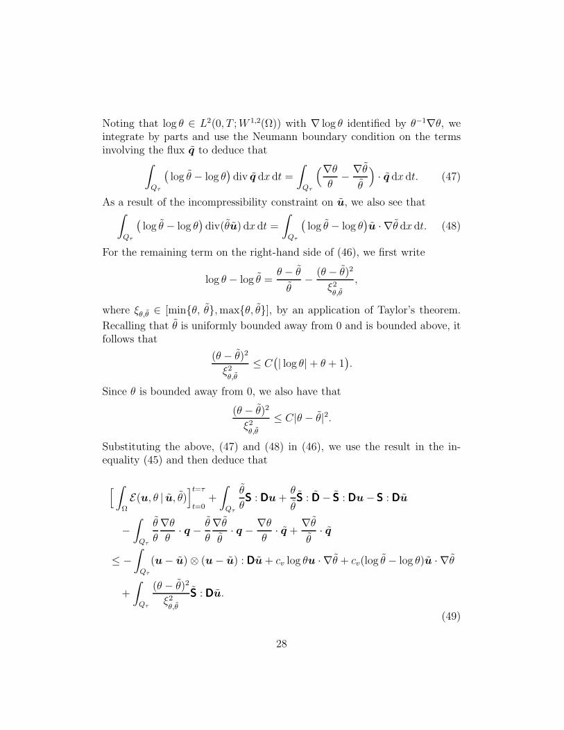
Noting that log θ ∈ L2(0, T ;W 1,2(Ω)) with ∇ log θ identified by θ−1∇θ, weintegrate by parts and use the Neumann boundary condition on the termsinvolving the flux q to deduce that
∫
Qτ
(
log θ − log θ)
div q dx dt =
∫
Qτ
(∇θ
θ−
∇θ
θ
)
· q dx dt. (47)
As a result of the incompressibility constraint on u, we also see that∫
Qτ
(
log θ − log θ)
div(θu) dx dt =
∫
Qτ
(
log θ − log θ)
u · ∇θ dx dt. (48)
For the remaining term on the right-hand side of (46), we first write
log θ − log θ =θ − θ
θ−
(θ − θ)2
ξ2θ,θ
,
where ξθ,θ ∈ [minθ, θ,maxθ, θ], by an application of Taylor’s theorem.
Recalling that θ is uniformly bounded away from 0 and is bounded above, itfollows that
(θ − θ)2
ξ2θ,θ
≤ C(
| log θ|+ θ + 1)
.
Since θ is bounded away from 0, we also have that
(θ − θ)2
ξ2θ,θ
≤ C|θ − θ|2.
Substituting the above, (47) and (48) in (46), we use the result in the in-equality (45) and then deduce that
[
∫
Ω
E(u, θ | u, θ)]t=τ
t=0+
∫
Qτ
θ
θSSS : DDDu+
θ
θSSS : DDD− SSS : DDDu− SSS : DDDu
−
∫
Qτ
θ
θ
∇θ
θ· q −
θ
θ
∇θ
θ· q −
∇θ
θ· q +
∇θ
θ· q
≤ −
∫
Qτ
(u− u)⊗ (u− u) : DDDu+ cv log θu · ∇θ + cv(log θ − log θ)u · ∇θ
+
∫
Qτ
(θ − θ)2
ξ2θ,θ
SSS : DDDu.
(49)
28

For the second and third terms on the right-hand side of (49), we have
−
∫
Qτ
cv log θu · ∇θ + cv(log θ − log θ)u · ∇θ dx dt
= −
∫
Qτ
cv log θ(u− u) · ∇θ + cv log θu · ∇θ dx dt
= −
∫
Qτ
cv log θ(u− u) · ∇θ dx dt
= −
∫
Qτ
cv(
log θ − log θ)
(u− u) · ∇θ dx dt.
Substituting this into (49), we get
[
∫
Ω
E(u, θ | u, θ) dx]t=τ
t=0+
∫
Qτ
θ
θSSS : DDDu+
θ
θSSS : DDDu− SSS : DDDu− SSS : DDDudx dt
−
∫
Qτ
θ
θ
∇θ
θ· q −
θ
θ
∇θ
θ· q −
∇θ
θ· q +
∇θ
θ· q dx dt
≤ −
∫
Qτ
(u− u)⊗ (u− u) : DDDu dx dt
−
∫
Qτ
cv(
log θ − log θ)
(u− u) · ∇θ dx dt +
∫
Qτ
(θ − θ)2
ξ2θ,θ
SSS : DDDudx dt
≤ ‖DDDu‖L∞(Qτ )‖u− u‖2L2(Qτ )+ ‖SSS‖L∞(Qτ )‖DDDu‖L∞(Qτ )
∫
Qτ
|θ − θ|2
ξ2θ,θ
dx dt
+ cv‖∇θ‖L∞(Qτ )‖ log θ − log θ‖L2(Qτ )‖u− u‖L2(Qτ ).
Next, we notice that
‖ log θ − log θ‖2L2(Qτ )=
∫
Qτ
[
| log θ − log θ|2]
ess+[
| log θ − log θ|2]
resdx dt
≤ C
∫
Qτ
[
|θ − θ|2]
ess+[
(log θ)2 + (log θ)2]
res
≤ C
∫
Qτ
[
|θ − θ|2]
ess+ [1 + θ]res dx dt
≤ C
∫
Qτ
E(u, θ | u, θ) dx dt,
29

where we use the fact that θ is uniformly bounded away from 0. Similarly,we have
‖u− u‖2L2(Qτ )≤ C
∫
Qτ
E(u, θ | u, θ) dx dt.
Furthermore, we see that∫
Qτ
|θ − θ|2
ξ2θ,θ
dx dt ≤
∫
Qτ
[ |θ − θ|2
ξ2θ,θ
]
ess+[ |θ − θ|2
ξ2θ,θ
]
resdx dt
≤ C
∫
Qτ
[
|θ − θ|2]
ess+[
1 + θ + | log θ|]
resdx dt
≤ C
∫
Qτ
E(u, θ | u, θ) dx dt.
It follows that[
∫
Ω
E(u, θ | u, θ) dx]t=τ
t=0+
∫
Qτ
θ
θSSS : DDDu+
θ
θSSS : DDDu− SSS : DDDu− SSS : DDDudx dt
−
∫
Qτ
θ
θ
∇θ
θ· q −
θ
θ
∇θ
θ· q −
∇θ
θ· q +
∇θ
θ· q dx dt
≤ C
∫
Qτ
E(u, θ | u, θ) dx dt.
(50)We aim to apply Gronwall’s inequality to (50) to deduce that
∫
Ω
E(u, θ | u, θ)(t) dx ≤(
∫
Ω
E(u0, θ0 | u0, θ0) dx)
eCt, (51)
where C is a constant that is independent of t. The required weak-stronguniqueness follows from this immediately by noticing that the right-handside vanishes when the initial data coincide. However, the second and thirdintegrals on the left-hand side of (50) are not necessarily non-negative. Thuswe cannot apply Gronwall’s inequality at present.
However, Under appropriate assumptions on κ and S as stated in As-sumption 3, we are able to bound the integrals from below in a suitable waysuch that (51) can be obtained. Using Fourier’s law, the constitutive relationconcerning the heat flux term, we see that
−
∫
Qτ
θ
θ
∇θ
θ· q −
θ
θ
∇θ
θ· q −
∇θ
θ· q +
∇θ
θ· q
30

=
∫
Qτ
θ
θ
∇θ
θ· κ(θ)∇θ −
θ
θ
∇θ
θ· κ(θ)∇θ −
∇θ
θ· κ(θ)∇θ +
∇θ
θ· κ(θ)∇θ
=
∫
Qτ
κ(θ)θ∣
∣
∣
∇θ
θ−
∇θ
θ
∣
∣
∣
2
− κ(θ)|∇θ|2
θ+ 2κ(θ)
∇θ
θ· ∇θ + κ(θ)
|∇θ|2
θ
− κ(θ)∇θ
θ· ∇θ − κ(θ)
∇θ
θ· ∇θ
=
∫
Qτ
κ(θ)θ∣
∣
∣
∇θ
θ−
∇θ
θ
∣
∣
∣
2
+|∇θ|2
θ
[
κ(θ)− κ(θ)]
+∇θ
θ· ∇θ
[
κ(θ)− κ(θ)]
=
∫
Qτ
κ(θ)θ∣
∣
∣
∇θ
θ−
∇θ
θ
∣
∣
∣
2
+∇θ ·[∇θ
θ−
∇θ
θ
]
[
κ(θ)− κ(θ)]
≥κ(θ)θ
2
∣
∣
∣
∇θ
θ−
∇θ
θ
∣
∣
∣
2
−|∇θ|2
2κ(θ)θ|κ(θ)− κ(θ)|2
Recalling that κ grows like θ12 for large θ and is locally Lipschitz, and using
the boundedness of θ, we see that
∫
Qτ
|∇θ|2
2κ(θ)θ|κ(θ)− κ(θ)|2 ≤ C
∫
Qτ
[
|κ(θ)− κ(θ)|2]
ess+[
|κ(θ)− κ(θ)|2]
res
≤ C
∫
Qτ
[
|θ − θ|2]
ess+[
1 + θ]
res
≤
∫
Qτ
E(u, θ | u, θ).
Substituting this bound into (50), we deduce that
[
∫
Ω
E(u, θ | u, θ)]t=τ
t=0+
∫
Qτ
θ
θSSS : DDDu+
θ
θSSS : DDDu− SSS : DDDu− SSS : DDDudx dt
+
∫
Qτ
|∇θ|2
2κ(θ)θ|κ(θ)− κ(θ)|2 dx dt
≤ C
∫
Qτ
E(u, θ | u, θ) dx dt.
(52)To deal with the second integral on the left-hand side of (52) we will
now make use of the strong monotonicity condition (37). Considering the
31

integrand in the aforementioned term, we write
θ
θSSS : DDDu+
θ
θSSS : DDDu− SSS : DDDu− SSS : DDDu
=θ
θ(SSS− SSS) : (DDDu−DDDu) + θ
(1
θ−
1
θ
)
SSS : DDDu+ θ(1
θ−
1
θ
)
SSS : DDDu
+ θ(1
θ−
1
θ
)
SSS : DDDu+ θ(1
θ−
1
θ
)
SSS : DDDu
=θ
θ(SSS− S(DDDu, θ)) : (DDDu−DDDu) +
θ
θ(S(DDDu, θ)− SSS) : (DDDu−DDDu)
+ θ(1
θ−
1
θ
)
SSS : (DDDu−DDDu) + θ(1
θ−
1
θ
)
DDDu : (SSS− SSS)
+(1
θ−
1
θ
)
(θ − θ)SSS : DDDu
≥θ
θc(
|SSS− SSS|2 + |DDDu−DDDu|2)
+θ
θ(S(DDDu, θ)− S(DDDu, θ)) : (DDDu−DDDu)
+ θ(1
θ−
1
θ
)
SSS : (DDDu−DDDu) + θ(1
θ−
1
θ
)
DDDu : (SSS− SSS)
+(1
θ−
1
θ
)
(θ − θ)SSS : DDDu.
The second term in the right-hand side can be dealt with by means of Young’sinequality, which yields
θ
θ(S(DDDu, θ)− S(DDDu, θ)) : (DDDu−DDDu) ≤ ǫ
θ
θ|DDDu−DDDu|2
+ C(ǫ)θ
θ|S(DDDu, θ)− S(DDDu, θ)|2,
where ǫ > 0 is a constant to be fixed sufficiently small later on. In a similarmanner, for the third and fourth terms on the right-hand side, we have
θ(1
θ−
1
θ
)
SSS : (DDDu−DDDu) + θ(1
θ−
1
θ
)
DDDu : (SSS− SSS)
=√
θθ(1
θ−
1
θ
)
√
θ
θSSS : (DDDu−DDDu) +
√
θθ(1
θ−
1
θ
)
√
θ
θDDDu : (SSS− SSS)
≤ ǫθ
θ
(
|DDDu−DDDu|2 + |SSS− SSS|2)
+ C(ǫ)(
‖SSS‖L∞(Qτ ) + ‖DDDu‖L∞(Qτ )
) |θ − θ|2
θθ.
32
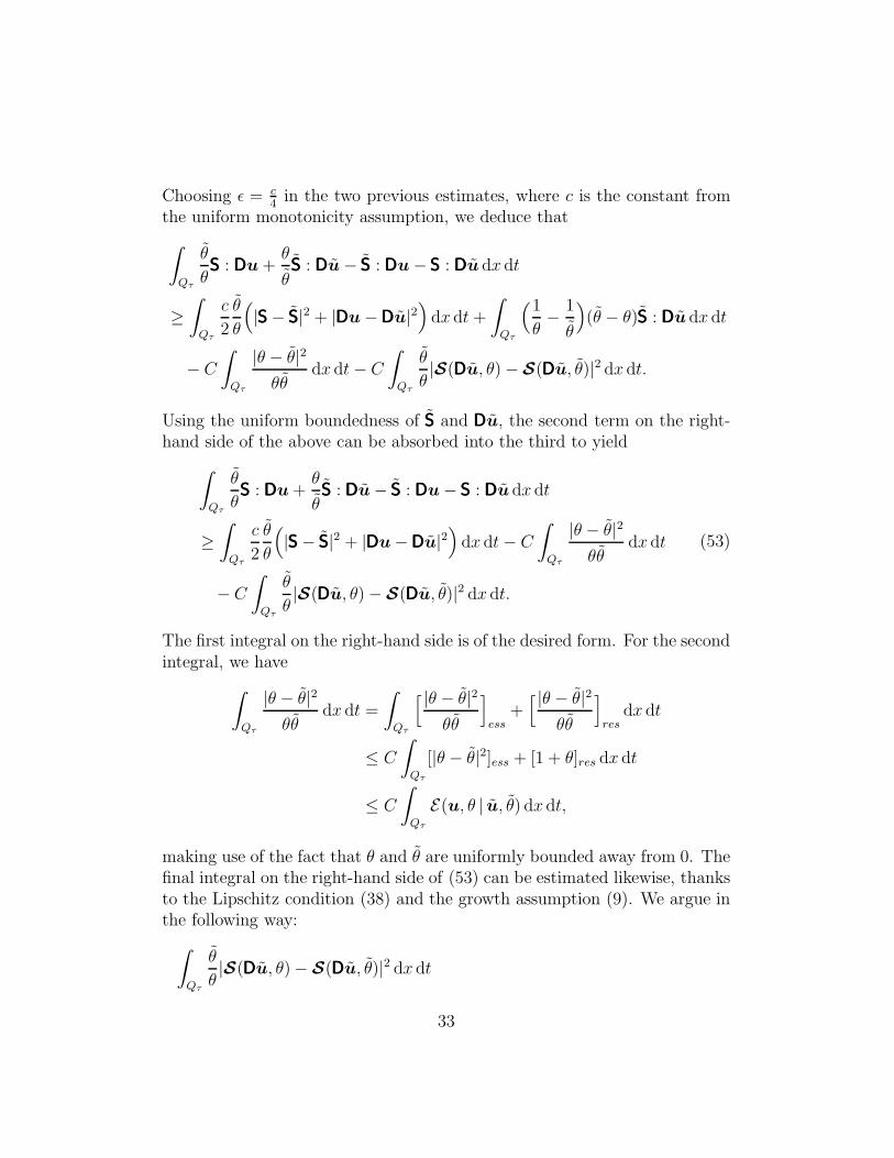
Choosing ǫ = c4in the two previous estimates, where c is the constant from
the uniform monotonicity assumption, we deduce that
∫
Qτ
θ
θSSS : DDDu+
θ
θSSS : DDDu− SSS : DDDu− SSS : DDDu dx dt
≥
∫
Qτ
c
2
θ
θ
(
|SSS− SSS|2 + |DDDu−DDDu|2)
dx dt +
∫
Qτ
(1
θ−
1
θ
)
(θ − θ)SSS : DDDudx dt
− C
∫
Qτ
|θ − θ|2
θθdx dt− C
∫
Qτ
θ
θ|S(DDDu, θ)− S(DDDu, θ)|2 dx dt.
Using the uniform boundedness of SSS and DDDu, the second term on the right-hand side of the above can be absorbed into the third to yield
∫
Qτ
θ
θSSS : DDDu+
θ
θSSS : DDDu− SSS : DDDu− SSS : DDDudx dt
≥
∫
Qτ
c
2
θ
θ
(
|SSS− SSS|2 + |DDDu−DDDu|2)
dx dt− C
∫
Qτ
|θ − θ|2
θθdx dt
− C
∫
Qτ
θ
θ|S(DDDu, θ)− S(DDDu, θ)|2 dx dt.
(53)
The first integral on the right-hand side is of the desired form. For the secondintegral, we have
∫
Qτ
|θ − θ|2
θθdx dt =
∫
Qτ
[ |θ − θ|2
θθ
]
ess+[ |θ − θ|2
θθ
]
resdx dt
≤ C
∫
Qτ
[|θ − θ|2]ess + [1 + θ]res dx dt
≤ C
∫
Qτ
E(u, θ | u, θ) dx dt,
making use of the fact that θ and θ are uniformly bounded away from 0. Thefinal integral on the right-hand side of (53) can be estimated likewise, thanksto the Lipschitz condition (38) and the growth assumption (9). We argue inthe following way:
∫
Qτ
θ
θ|S(DDDu, θ)− S(DDDu, θ)|2 dx dt
33

≤ C
∫
Qτ
[
|S(DDDu, θ)− S(DDDu, θ)|2]
ess+[
|S(DDDu, θ)− S(DDDu, θ)|2]
resdx dt
≤ C(‖DDDu‖L∞(Qτ ))
∫
Qτ
[|θ − θ|2]ess + [1]ess dx dt
≤ C
∫
Qτ
E(u, θ | u, θ) dx dt,
using the Lipschitz property of S to deal with the essential part and growthcondition on S to bound the residual part.
It follows that
[
∫
Ω
E(u, θ | u, θ) dx]t=τ
t=0+
∫
Qτ
θ
θ
(
|SSS− SSS|2 + |DDDu−DDDu|2)
dx dt
+
∫
Qτ
(1
θ−
1
θ
)
(θ − θ)SSS : DDDu dx dt
≤ C
∫
Qτ
E(u, θ | u, θ) dx dt.
Applying Gronwall’s inequality, we conclude the required result. We notethat the existence of strong solutions for small data has been obtained in[34] (see also [35]); under such assumptions we would then have that thenumerical approximations devised in Proposition 1 would converge to thestrong solution.
Some examples of constitutive relations satisfying the assumptions re-quired in this section, in particular the strong monotonicity (37), include theCarreau–Yasuda constitutive relation for r < 2, given by
SSS = α(θ)DDDu+ β(θ)(1 + Γ(θ)|DDDu|2)r−22 DDDu, (54)
where α, β and Γ are locally Lipschitz continuous functions satisfying 0 <c1 ≤ α, β,Γ ≤ c2, for two positive constants c1, c2 > 0. Although theHerschel–Bulkley constitutive relation (35) is not strongly monotone, in prac-tice it is common to regularise it when performing numerical approximations,in order to deal with its non-differentiable character. We mention for exam-ple, that the following regularisation (introduced in [36])
GGG(SSS− εDDDu,DDDu− εSSS) = 0, (55)
which can be applied to the expression (36), leads to a relation satisfying thestrong monotonicity condition (37), even if r 6= 2 [36, Eq. 4.26].
34
Remark 5. The weak-strong uniqueness result for the isothermal systemobtained in [23] only requires that r > 1 and surprisingly does not impose theconstitutive relation pointwise at the level of the dissipative weak solutions.One consequence is that the result has to account for possible concentrationsin the convective term div(u⊗ u). An extension of the results presented inthis paper to a setting with such relaxed assumptions will be the subject offuture work. In the current non-isothermal setting, the assumption r > 1would also lead to potential concentrations in the advective term for theentropy div(Su). On the other hand, since the constitutive relation wouldnot need to be identified pointwise, a discrete parabolic Lipschitz truncationwould not be necessary, which means that the penalty term (and so the indexk) could be dropped from the approximation scheme.
Remark 6. The notion of dissipative weak solution introduced in Definition1 is suitable for energetically isolated systems with u|∂Ω = 0 and q|∂Ω =0. The case of Dirichlet boundary conditions for the temperature θ|∂Ω =θb is therefore excluded; this problem has only recently been solved in thecompressible case in [37]. In this case it was necessary to modify the balanceof total energy (6d) and employ instead the so-called ballistic free energy. Itseems plausible that these arguments carry over to the incompressible settingand will be the subject of future research.
References
[1] Y. Kagei, On weak solutions of nonstationary Boussinesq equations,Differential Integral Equations 6 (3) (1993) 587–611.
[2] J. Malek, M. Ruzicka, G. Thater, Fractal dimension, attractors, andthe Boussinesq approximation in three dimensions, Acta Appl. Math.37 (1-2) (1994) 83–97.
[3] T. Hishida, Y. Yamada, Global solutions for the heat convection equa-tions in an exterior domain, Tokyo J. Math. 15 (1992) 135–151.
[4] J. I. Dıaz, G. Galiano, Existence and uniqueness of solutions of theBoussinesq system with nonlinear thermal diffusion, Topol. MethodsNonlinear Anal. 11 (1) (1998) 59–82.
[5] J. Necas, T. Roubicek, Buoyancy-driven viscous flow with L1-data, Non-linear Anal. 46 (2001) 737–755.
35

[6] J. Naumann, On the existence of weak solutions to the equations ofnon-stationary motion of heat-conducting incompressible viscous fluids,Mathematical methods in the applied sciences 29 (16) (2006) 1883–1906.
[7] T. Clopeau, A. Mikelic, Nonstationary flows with viscous heating effects,in: Elasticite, viscoelasticite et controle optimal, ESAIM Proc., vol. 2,1997, pp. 55–63.
[8] L. Consiglieri, Weak solutions for a class of non-Newtonian fluids withenergy transfer, J. Math. Fluid Mech. 2 (3) (2000) 267–293.
[9] M. Bulıcek, E. Feireisl, J. Malek, A Navier-Stokes-Fourier system forincompressible fluids with temperature dependent material coefficients,Nonlinear Anal. Real World Appl. 10 (2009) 992–1015.
[10] E. Feireisl, J. Malek, On the Navier–Stokes equations with temperature-dependent transport coefficients, Differ. Equ. Nonlinear Mech. (90616)(2006) 1–14.
[11] M. Bulıcek, J. Malek, K. R. Rajagopal, Mathematical analysis of un-steady flows of fluids with pressure, shear-rate, and temperature depen-dent material moduli that slip at solid boundaries, SIAM J. Math. Anal.41 (2) (2009) 665–707.
[12] E. Maringova, J. Zabensky, On a Navier–Stokes–Fourier-like systemcapturing transitions between viscous and inviscid fluid regimes andbetween no-slip and perfect-slip boundary conditions, Nonlinear Anal.Real World Appl. 41 (2018) 152–178.
[13] E. Feireisl, A. Novotny, Weak-strong uniqueness property for the fullNavier–Stokes–Fourier system, Arch. Ration. Mech. Anal. 204 (2012)683–706.
[14] E. Feireisl, B. J. Jin, A. Novotny, Relative entropies, suitable weak so-lutions, and weak-strong uniqueness for the compressible Navier–Stokessystem, J. Math. Fluid Mech. 14 (4) (2012) 717–730.
[15] J. Brezina, E. Feireisl, A. Novotny, Stability of strong solutions to theNavier–Stokes–Fourier system, SIAM J. Math. Anal. 52 (2) (2020) 1761–1785.
36
[16] L. Saint-Raymond, Hydrodynamic limits: some improvements of therelative entropy method, Annal. I. H. Poincare - AN 26 (3) (2009) 705–744.
[17] S. Demoulini, D. M. A. Stuart, A. E. Tzavaras, Weak-strong uniquenessof dissipative measure-valued solutions for polyconvex elastodynamics,Arch. Ration. Mech. Anal. 205 (3) (2012) 927–961.
[18] C. Lattanzio, A. E. Tzavaras, Relative entropy in diffusive relaxation,SIAM J. Math. Anal. 45 (3) (2013) 1563–1584.
[19] A. Abbatiello, E. Feireisl, A. Novotny, Generalized solutions to modelsof compressible viscous fluids, ArXiv Preprint: 1912.12896 (2019).
[20] G. Prodi, Un teorema di unicita per le equazioni di Navier–Stokes, Ann.Mat. Pura Appl. 48 (1959) 173–182.
[21] J. Serrin, On the interior regularity of weak solutions of the Navier–Stokes equations, Arch. Ration. Mech. Anal. 9 (1962) 187–195.
[22] E. Wiedemann, Weak-strong uniqueness in fluid dynamics. Partial Dif-ferential Equations in fluid mechanics, Vol. 452 of London Math. Soc.Lecture Note Ser., Cambridge Univ. Press, 2018, pp. 289–326.
[23] A. Abbatiello, E. Feireisl, On a class of generalized solutions to equationsdescribing incompressible viscous fluids, Ann. di Mat. Pura ed Appl. 199(2020) 1183–1195. doi:10.1007/s10231-019-00917-x.
[24] E. Feireisl, M. Lukacova-Medvid’ova, H. Mizerova, B. She, Convergenceof a finite volume scheme for the compressible Navier–Stokes system,ESAIM: M2AN 53 (6) (2019) 1957–1979.
[25] Y. Li, B. She, On convergence of numerical solutions for the compress-ible MHD system with exactly divergence-free magnetic field, ArXivPreprint: 2107.01369 (2021).
[26] T. Roubicek, Nonlinear Partial Differential Equations with Applications,2nd Edition, Birkhauser, 2013.
[27] V. Girault, P. A. Raviart, Finite Element Methods for Navier-StokesEquations: Theory and Algorithms, Springer Verlag, 1986.
37

[28] P. E. Farrell, P. A. Gazca-Orozco, E. Suli, Numerical analysis of un-steady implicitly constituted incompressible fluids: 3-field formulation,SIAM J. Numer. Anal. 58 (1) (2020) 757–787. arXiv:1904.09136.
[29] E. Suli, T. Tscherpel, Fully discrete finite element approximation ofunsteady flows of implicitly constituted incompressible fluids, IMA J.Numer. Anal. dry097 (2019). doi:10.1093/imanum/dry097.
[30] J. Blechta, J. Malek, K. R. Rajagopal, On the classification of in-compressible fluids and a mathematical analysis of the equations thatgovern their motion, SIAM J. Math. Anal. 52 (2) (2020) 1232–1289.doi:10.1137/19M1244895.
[31] J. W. Glen, The creep of polycrystalline ice, Proc. R. Soc. A-Math.Phys. Eng. Sci. 228 (1175) (1955) 519–538.
[32] P. E. Farrell, P. A. Gazca-Orozco, E. Suli, Finite element approxi-mation and augmented Lagrangian preconditioning for anisothermalimplicitly-constituted non-Newtonian flow, Math. Comp. (in press).ArXiv Preprint: 2011.03024 (2021).
[33] L. Diening, C. Kreuzer, E. Suli, Finite element approximationof steady flows of incompressible fluids with implicit power-law-like rheology, SIAM J. Numer. Anal. 51 (2) (2013) 984–1015.doi:10.1137/120873133.
[34] H. Amann, Heat-conducting incompressible viscous fluids, Navier–Stokes Equations and Related Nonlinear Problems, Plenum Press, NewYork, 1995, pp. 231–243.
[35] M. Benes, Strong solutions to non-stationary channel flows of heat-conducting viscous incompressible fluids with dissipative heating, ActaAppl. Math. 116 (3) (2011) 237–254.
[36] M. Bulıcek, J. Malek, E. Maringova, On nonlinear problems of parabolictype with implicit constitutive equations involving flux, ArXiv Preprint:2009.06917 (2020).
[37] N. Chaudhuri, E. Feireisl, Navier–Stokes–Fourier system with Dirichletboundary conditions, ArXiv Preprint: 2106.05315 (2021).
38