wealth and poverty revisited - senate

by

Richard K. Vedder andLowell E. Gallaway

Distinguished Professors of Economics,Ohio University

Joint Economic Committee1537 Longworth House Office BuildingWashington, DC 20515Phone: 202-226-3234Fax: 202-226-3950

Internet Address:http://www.house.gov/jec

WEALTH AND POVERTY REVISITED

Prepared for theJoint Economic Committee

Jim Saxton (R-NJ), Chairman

May 2001

G-01 Dirksen Senate Office BuildingWashington, DC 20510Phone: 202-224-5171Fax: 202-224-0240

Executive Summary

There are compelling arguments for promoting moderation in the growth of governmental expenditures over time. A potentially politically viable policy for promoting economic growth would be to allow government expenditures to rise modestly over time, but by less than the growth rate in GDP, leading in time to some reduction in governmental expenditures as a percent of GDP. In effect, this has been the experience of the past several years. In addition, the benefits of moderating inflation observed in recent times are arguments for the Federal Reserve continuing to follow its stated objective of promoting price stability. Since taxes tend to automatically rise over time as a percent of GDP (in large part, because of the progressive nature of the income tax), and since tax reduction also tends to reduce the propensity of policy-makers to increase expenditure, a very strong case can be made for a tax cut. Current softness in the economy further supports the case for tax reduction.

WEALTH AND POVERTY REVISITED By Richard Vedder and Lowell Gallaway1

INTRODUCTION

The last two decades of American economic history have been characterized by rising incomes, consumption and wealth, and also by some decline in the rate of poverty. The nation has had the benefit of economic expansion for about 95 percent of the time since 1983, the largest proportion of time devoted to expansion for any 17-18 year period since records are available (1854). While problems of data aggregation, measuring inflation and so forth are real, there is no doubt that the standard of living of Americans is at an historic high, and that the rate of growth of income and consumption per capita after adjusting for inflation compares favorably with much of modern American history.

The modern experience tells us that economic change is often fairly complex, and that uni-causal

theories of economic growth seldom fully explain all the determinants of rising incomes and wealth. At the same time, however, there is strong evidence that large portions of the differences in economic performance between nations are explainable in terms of a few key variables determined by public policy. For example, hardly any one today would disagree that the major reason for the differences in growth between North and South Korea is that the former region has adopted public policies that prohibit private entrepreneurship and thwart the powerful resource allocation capabilities of markets, while South Korea has embraced market capitalism. Similarly, most observers would agree that the economic success in Poland, Hungary and the Czech Republic relative to Russia in the past decade reflects the fact that the smaller nations, with a more recent capitalist past, have been quicker to embrace market capitalism with the attendant institutional protection of property rights coupled with a strong rule of law. Other similar illustrations abound. To cite one last example, the economic success of Thailand, Malaysia and Singapore relative to Myanamar (Burma) or Vietnam again largely reflects differential rates of acceptance of market capitalism, with it being embraced to a large extent in the former countries, but far less so in the latter.

Even within western capitalistic democracies, the degree to which the private capitalistic sector

allocates resources using the market mechanism is an important factor in explaining differential economic performance. Compare, for example, the United States and Sweden. In 1970, per capita total output was by some measures significantly less in the United States than in Sweden.2

Today, output per capita in the U.S. exceeds that in Sweden by 14 to 47 percent, depending on

the measure used.3 This rising differential, we strongly suspect, is a consequence of radically different 1The authors are Distinguished Professors of Economics at Ohio University. 2 For example, in constant 1977 dollars, the 1970 real gross national product per capita in Sweden was $9,012, more than 20 percent higher than the U.S. figure of $7,428. See U.S. Bureau of the Census, Statistical Abstract of the United States:1981, p. 878. These data were computed using the exchange rate method; the use of the purchasing parity power method shows a more favorable U.S. economy relative to Sweden. 3 In 1998, per capita gross national product using the exchange rate method was $29,240 in the U.S. and $25,580 in Sweden; using the purchasing power parity method, the U.S. figure was $29,240, and the Swedish figure was $19,848. See U.S. Bureau of the Census, Statistical Abstract of the United States:2000, p. 831.

A JOINT ECONOMIC COMMITTEE STUDY

public policies. Using government spending as a percent of total output as a measure of state intervention in market processes, in the United States that intervention has increased modestly since 1970, while in Sweden it has soared, with spending now approximating 60 percent of total output compared with 35 percent or so in the United States. Similarly, whereas in Europe, France, Germany, and Italy far outdistanced Great Britain as late as the 1970s by most economic indicators, in the 1990s the reverse was the truth, with the change largely explainable by the much larger growth in state involvement in the economies in the continental countries than in Britain.4

To be sure, rising material success has not meant an end to poverty for all, even in the world’s

richest major nation, the United States. Some would argue that rising per capita income has been accompanied by greater income inequality, so the poor remain numerous and increasingly alienated from society. Yet an objective evaluation of the evidence suggests that attempts to eradicate poverty by interfering with the “invisible hand” of the market economy often are self-defeating.

In this study, we look at the determinants of wealth and poverty in the United States in modern

times. We will argue that the private market economy is a better creator of wealth than the most viable alternative, namely the modern interventionist welfare state. Moreover, the modern historical experience is that the welfare state has severe limitations in doing what many consider its first duty, eliminating poverty. The sharp rise in wealth until recently and the reduction in poverty in recent years reflects in part the retreat of the welfare state, along with relative stability in a critical factor in market resource allocation decisions, namely prices.

GOVERNMENT AND THE CREATION OF WEALTH As Figure 1 indicates, real wealth per capita has grown sharply in the United States over time.

There is no growth from 1945 to 1953, a period during which price indices to calculate real wealth are extremely suspect owing to wartime price controls of World War II and the Korean War. Starting our analysis in 1953, real wealth per capita more than tripled in the next 46 years, rising by 2.57 percent per year - more than the growth in real output per capita, meaning that the wealth-income ratio rose over time.5 If anything, this understates wealth growth because of the general agreement amongst professional economists that the CPI-U used to convert nominal dollars to real constant dollars overstates inflation.

Wealth is created in many ways. People save and accumulate assets in financial institutions, and

they also invest in real property. Since a large proportion of wealth represents ownership interest in corporations and businesses, indirectly business savings impacts household wealth. Finally, the market value of assets deviates from book or historic values in part because of changing expectations as to the

4 From 1976 through 1980, the compounded annual growth rate in real GNP was 4.8 percent in Italy, 3.3 percent in Germany, 3.1 percent in France, and only 1.9 percent in Great Britain. From 1991 through 2000, the annual growth rate in real GDP was 2.6 percent in Britain, 1.8 percent in France, and 1.5 percent in both Germany and Italy. Authors’ calculations from data in the Economic Report of the President: 2001, p. 402, and the Economic Report of the President:1987, p. 368. 5Wealth data are from the Board of Governors, Federal Reserve System, Flow of Funds Accounts, from the balance sheets for households and non-profit organizations. Population data are from the U.S. Bureau of the Census. Data are deflated by the Consumer Price Index for All Urban Consumers (CPI-U). http://www.federalreserve.govhttp://www.bls.gov.

WEALTH AND POVERTY REVISITED PAGE 3

utility of the assets, particularly with respect to the earning power of equity interests of businesses. In periods of prosperity and optimism, wealth rises faster than otherwise, because the anticipated present value of future profits or income increases.

How does public policy impact on wealth creation? Given our earlier discussion, other things

equal, we would a expect a rise in governmental expenditures relative to national output should lead to a decline in wealth. If government spending is growing relative to income or output, the burden of government on the private sector grows, lowering the private rate of return from property. To claim more resources, government crowds out private sector activities, including wealth creation in the form of investment. Moreover, the market price of existing assets should decline as the remuneration to those assets falls because of increased taxes, if government is so financed, or higher inflation or interest rates if it is financed through borrowing.

Public policy can effect wealth through monetary policy and its impact on prices. Inflation is

largely a monetary phenomenon, caused when the money supply grows faster than output. The creation of money is controlled by a public entity, the Federal Reserve System. Secondarily, expansionary fiscal policy financed through borrowing likewise can be inflationary, particularly when it reflects the monetization of debt by the central bank.

In terms of financial markets, inflation lowers the nominal (not to mention real) value of paper

securities. If a person buys a bond for $1000 that has $60 in annual interest payments, the nominal yield is six percent a year. Suppose inflation increases, meaning the real value of the $60 annual interest payment falls. The market price of the bond will fall reflecting its declining attractiveness, raising the nominal yield. As bond prices fall, bonds become more attractive as an investment vehicle than otherwise, and some persons will sell stocks to buy bonds, depressing stock prices as well. Thus inflation should, other things equal, lower real wealth in the form of bonds or stocks, not to mention deposit accounts in financial institutions. Moreover, inflation reduces the efficiency of the market signals which lead to shifts in resource allocation. When prices are stable, rising prices in one sector denote rising demand and/or falling supply for that sector’s goods or services, but when prices are rising throughout the economy, it is less clear that the rising prices in a given sector reflect changing demand or supply for that sector’s products or simply the impact of general inflation. The information that price changes convey for the purpose of resource allocation is reduced or distorted when overall prices are rising. Also, inflation forces scarce human resources to engage in strategies designed to offset inflation’s impact, further lowering output from what otherwise would be the case.

Summarizing, we hypothesize that the wealth of individuals is lowered when government grows

relative to the economy as a whole, and also falls when the rate of inflation rises. An alternative way of stating it is that wealth is enhanced by keeping government limited and prices stable.

STATISTICAL EVIDENCE ON THE WEALTH-INFLATION-GROWTH RELATIONSHIP Data are available allowing for the testing of the hypothesis. As a measure of governmental size,

we used governmental (both federal and state and local) current expenditure as a percent of gross


domestic product, from national income accounts data of the Bureau of Economic Analysis of the U.S. Department of Commerce. In our results below, this is referred to as GOVGDP. Figure 2 shows trends in that data over time. Note that from the mid-1950s to the md-1970s, there was a sharp upward trend. While the movements in the series are more mixed after the mid-1970s, on balance they are upward until a peak is reached at over 32 percent in 1992, before a significant decline begins.

As our measure of inflation, we used the percentage annual change in the CPI-U (CHCPI). As

indicated, the real wealth per capita data (NETWORTH) were derived by dividing the net worth of households and non-profit organizations by population, and then converting numbers to constant dollars using the CPI-U. Because the real-wealth data had a positive trend, causing potential econometric problems of non-stationarity, we report two sets of results, one using the data as indicated, and the second where we converted the numbers to first difference form, relating the percent change in real net worth per capita (CHNETWORTH) to the change in the percent of GDP accounted for by government expenditures (CGOVGDP) and the percentage point change in the growth in the CPI-U (CHCHCPI). In the original model, we introduce as a control variable the level of real gross domestic product, RGDP. We examined the 47 year period 1953 through 1999.

Looking first at the initial results, we obtain: (1) NETWORTH = 30955.59 + 8.68 RGDP - 666.41 GOVGDP - 435.23 CHCPI, (3.54) (11.02) (2.10) (2.66)

_ R2 = .983, D-W = 1.62, F-Statistic = 665.41,

where the numbers in parentheses are t-values of the relevant variables. The results are relatively robust, with the model having a high predictive power and all variables significant in the expected direction at least the five percent level. Higher GOVGDP and CHCPI are associated with lower real net worth per capita. Bigger government and inflation are negatively related to wealth, controlling for the size of aggregate output (RGDP). At the margin, each one percentage point growth in federal spending as a percent of GDP, other things equal, is estimated to reduce per capita wealth by over $666, expressed in dollars of 1982-84 purchasing power, which is well over one thousand dollars today. Similarly, other things equal, a one percent rise in prices is associated with over a $435 wealth decline expressed in 1982-84 dollars, or well over $700 in current dollars.

While the above results are strong, they have some underlying weaknesses econometrically,

weaknesses that are mitigated by the use of the second model discussed above: (2) CHNETWORTH = 5.881 - 1.435 CGOVGDP - 0.475 CHCPI, (8.30) (2.23) (3.22)

_ R2 = .307, D-W = 1.87, F-Statistic = 5.08.


While this alternative model is statistically far less robust, the hypothesized negative

relationships between changes in real wealth and changes in the relative size of government and changing amounts of inflation are maintained and are statistically significant at the five percent level.

It is possible to disaggregate governmental spending data somewhat. For example, does the

conclusion above hold if one confines the analysis exclusively to federal spending as a percent of GDP? What about state and local spending? Replicating regressions (1) and (2) but substituting federal spending as a percent of GDP and then state and local spending as a percent of GDP is interesting. In the two federal regressions, there is a negative relationship observed between federal spending as a percent of GDP and net worth, one statistically significant at the five percent, and the second at the 10 percent level. Only one of the two state regressions is statistically significant and negative. The evidence is stronger that federal spending has an adverse impact on wealth creation than state and local spending.

Wealth seems to be adversely impacted by a growth in the relative size of government or by

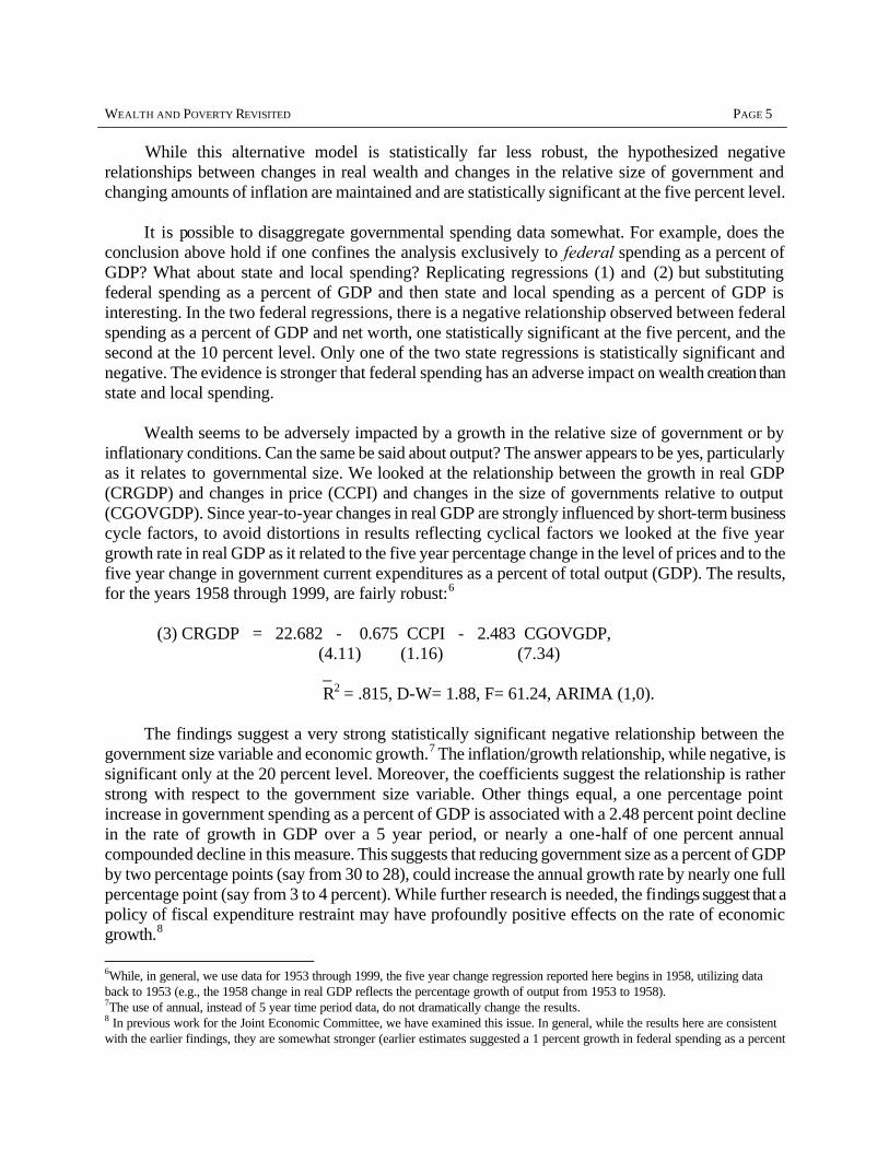
inflationary conditions. Can the same be said about output? The answer appears to be yes, particularly as it relates to governmental size. We looked at the relationship between the growth in real GDP (CRGDP) and changes in price (CCPI) and changes in the size of governments relative to output (CGOVGDP). Since year-to-year changes in real GDP are strongly influenced by short-term business cycle factors, to avoid distortions in results reflecting cyclical factors we looked at the five year growth rate in real GDP as it related to the five year percentage change in the level of prices and to the five year change in government current expenditures as a percent of total output (GDP). The results, for the years 1958 through 1999, are fairly robust:6

(3) CRGDP = 22.682 - 0.675 CCPI - 2.483 CGOVGDP, (4.11) (1.16) (7.34) _ R2 = .815, D-W= 1.88, F= 61.24, ARIMA (1,0). The findings suggest a very strong statistically significant negative relationship between the

government size variable and economic growth.7 The inflation/growth relationship, while negative, is significant only at the 20 percent level. Moreover, the coefficients suggest the relationship is rather strong with respect to the government size variable. Other things equal, a one percentage point increase in government spending as a percent of GDP is associated with a 2.48 percent point decline in the rate of growth in GDP over a 5 year period, or nearly a one-half of one percent annual compounded decline in this measure. This suggests that reducing government size as a percent of GDP by two percentage points (say from 30 to 28), could increase the annual growth rate by nearly one full percentage point (say from 3 to 4 percent). While further research is needed, the findings suggest that a policy of fiscal expenditure restraint may have profoundly positive effects on the rate of economic growth.8

6While, in general, we use data for 1953 through 1999, the five year change regression reported here begins in 1958, utilizing data back to 1953 (e.g., the 1958 change in real GDP reflects the percentage growth of output from 1953 to 1958). 7The use of annual, instead of 5 year time period data, do not dramatically change the results. 8 In previous work for the Joint Economic Committee, we have examined this issue. In general, while the results here are consistent with the earlier findings, they are somewhat stronger (earlier estimates suggested a 1 percent growth in federal spending as a percent


The results to this point suggest that the classical liberal prescription of limited government and

stable prices have much to commend them, both with respect to wealth and income creation. The analysis can be carried one step further. Income or output are flows created in the current time period from existing resources. Wealth is a stock concept, the valuation placed on productive resources, reflecting market perceptions as to the present value of future output (and profits) to be created. Those perceptions may be more volatile than the fluctuations in output itself, a fact confirmed because the coefficient of variation on changes in real net worth is significantly greater than the same coefficient with respect to changes in real gross domestic product.9 Does the volatility in wealth valuations reflect changes in public policy? Can public policies that are perceived as adverse to wealth creation lower expectations about the future and measurably impact on the wealth of citizens?

Before proceeding with empirical analysis, we would note that in recent years the wealth-

income ratio has risen, and is at a postwar high (see Figure 3). Casual empiricism would note that the sharp rise in the wealth-income ratio in the late 1990s was associated with both relatively modest (and stable) rates of inflation and, even more importantly, a significant decline in government expenditures as a percent of GDP (GOVGDP). GOVGDP fell for seven consecutive years, a continuous decline of the longest duration in modern American economic history.

An interesting statistical test can help tell us if public policy in fact influences the wealth-income

ratio as “eyeballing” the data suggests. We would hypothesize that while expansions in the relative size of government and the rate of inflation seem to have adverse effects on both income and wealth creation, the effects are greater on wealth creation, since not only is wealth reduced because of the decline in the present value of future income flows valued at lower amounts of income because of the adverse public policies, but also because excessive government/inflation increases perceived and/or actual risks to investments and thus lowers values of future assets.

To test the hypothesis, we ran four regressions, not reported here for reasons of space. We used

two different measures of the wealth-output (or wealth-income) ratio. First, we looked at the nominal net worth of households divided by nominal gross domestic product, and, second, real net worth per capita divided by real gross domestic product per capita. If the same price index is used to deflate both net worth and GDP, the two series would be the same, but, as is customary, we used the GDP price deflator of the Department of Commerce to obtain real GDP (and then divided it by population), and used the CPI-U of the Department of Labor to obtain real net worth. Since these two price indices are not identical and behave somewhat differently, the trends in the wealth-income ratio are somewhat different, although both measures find that that ratio hit a low in the postwar period in 1974, and a high

of GDP might lower growth by about O.15 percentage points a year, about one-third the magnitude estimate here). See Richard Vedder and Lowell Gallaway, “Government Size and Economic Growth,” (Study, Joint Economic Committee of Congress, December 1998). For another JEC study reaching similar conclusions but using somewhat different methodology, see James Gwartney, Robert Lawson and Randall Holcombe, “The Size and Functions of Government and Economic Growth (Study, Joint Economic Commitee of Congress, April 1998). For earlier work by us on this issue, see Lowell Gallaway and Richard Vedder, “The Impact of he Welfare State on the American Economy,” JEC Study, December 1995. All the above studies are available at the JEC web site: http://www.house.gov/jec. Additionally, we would note that the government spending/economic growth relationship is probably not linear, and that at lower levels of spending, such spending might be growth-enhancing (a positive relationship). See our “Government Size and Economic Growth” for details. 9 In the period 1953-99, the coefficient of variation (standard deviation divided by the arithmetic mean) for percent changes in real gross domestic product was 0.691, compared with 1.091 for percent changes in real net worth.


in 1999. As expected, the two wealth-income series are positively correlated with each other in a statistically significant fashion. We also used two time periods for our analysis: 1953-99, and 1974-99 (the latter period from the postwar low to the postwar high in the wealth-income ratio).

In all four regressions, the hypothesized negative relationship between government spending as a

percent of GDP and the wealth-income ratio was observed, and in three of them it was significant at the 10 percent level, and in two of them at the five percent level. The hypothesized negative relationship between the inflation rate and the wealth-income ratio was observed in all regressions, and was consistently significant at least at the five percent level. This strengthens our conviction that excessive government and inflation have negative effects on both wealth and income, but especially on wealth: investor confidence is shaken by governmental programs (and the taxes that typically finance them) that crowd out private spending, and by inflationary policies.

STOCK MARKET WEALTH AND PUBLIC POLICY A significant part of the rise in real net worth in recent times is attributed to the sharp increases

in stock prices after 1994. In that year, less than 14 percent of household assets were in the form of “corporate equities” or “mutual fund shares.” More than 38 percent of the increase in household assets from 1994 to 1998 were in these two categories, and if the “pension fund reserves” (most of which are typically invested in equities) are included, the proportion rises to well above 60 percent. The rise in the stock market has fueled a majority of the recent upsurge in wealth.

Does stock market wealth respond in the same fashion to public policies relating to government

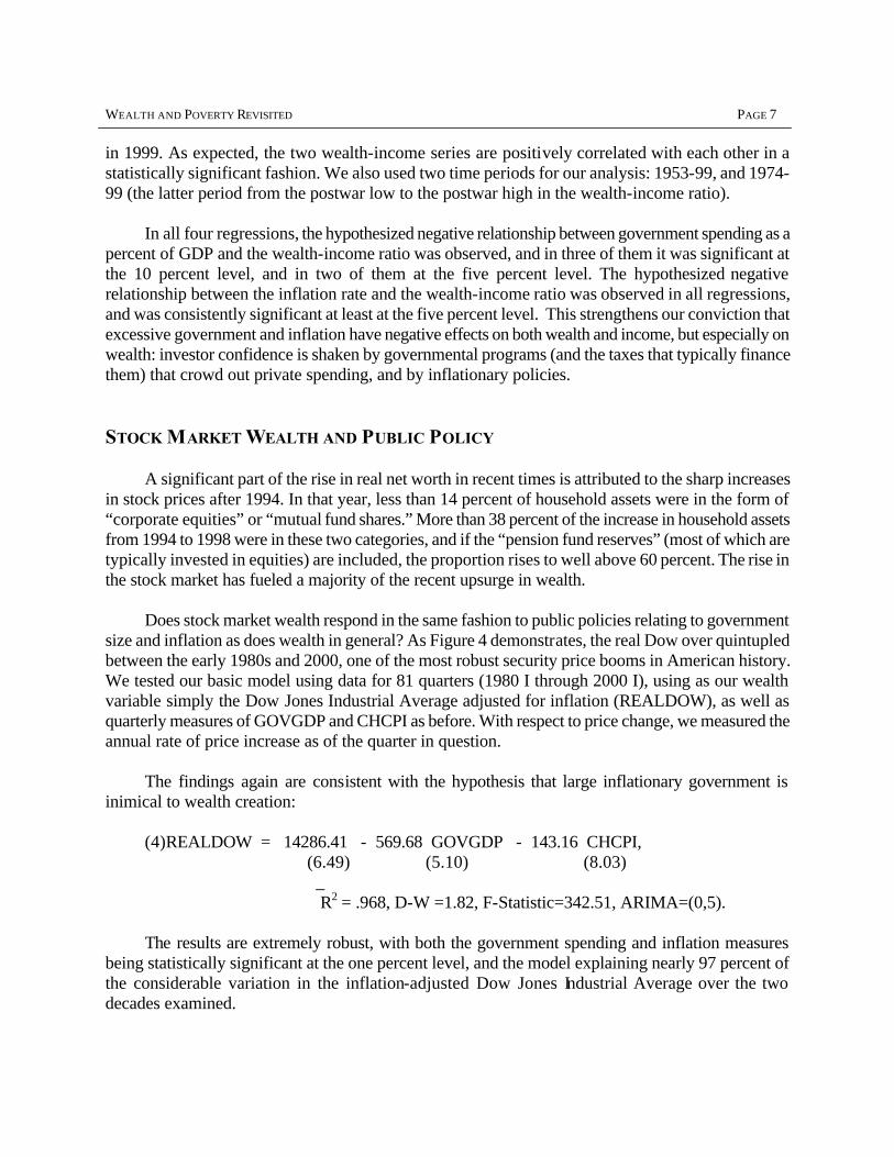
size and inflation as does wealth in general? As Figure 4 demonstrates, the real Dow over quintupled between the early 1980s and 2000, one of the most robust security price booms in American history. We tested our basic model using data for 81 quarters (1980 I through 2000 I), using as our wealth variable simply the Dow Jones Industrial Average adjusted for inflation (REALDOW), as well as quarterly measures of GOVGDP and CHCPI as before. With respect to price change, we measured the annual rate of price increase as of the quarter in question.

The findings again are consistent with the hypothesis that large inflationary government is

inimical to wealth creation: (4)REALDOW = 14286.41 - 569.68 GOVGDP - 143.16 CHCPI, (6.49) (5.10) (8.03) _ R2 = .968, D-W =1.82, F-Statistic=342.51, ARIMA=(0,5). The results are extremely robust, with both the government spending and inflation measures

being statistically significant at the one percent level, and the model explaining nearly 97 percent of the considerable variation in the inflation-adjusted Dow Jones Industrial Average over the two decades examined.


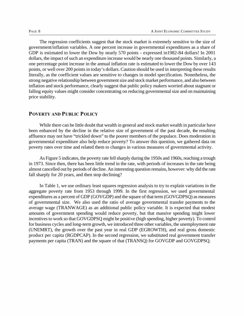
The regression coefficients suggest that the stock market is extremely sensitive to the size of

government/inflation variables. A one percent increase in governmental expenditures as a share of GDP is estimated to lower the Dow by nearly 570 points - expressed in1982-84 dollars! In 2001 dollars, the impact of such an expenditure increase would be nearly one thousand points. Similarly, a one percentage point increase in the annual inflation rate is estimated to lower the Dow by over 143 points, or well over 200 points in today’s dollars. Caution should be used in interpreting these results literally, as the coefficient values are sensitive to changes in model specification. Nonetheless, the strong negative relationship between government size and stock market performance, and also between inflation and stock performance, clearly suggest that public policy makers worried about stagnant or falling equity values might consider concentrating on reducing governmental size and on maintaining price stability.

POVERTY AND PUBLIC POLICY While there can be little doubt that wealth in general and stock market wealth in particular have

been enhanced by the decline in the relative size of government of the past decade, the resulting affluence may not have “trickled down” to the poorer members of the populace. Does moderation in governmental expenditure also help reduce poverty? To answer this question, we gathered data on poverty rates over time and related them to changes in various measures of governmental activity.

As Figure 5 indicates, the poverty rate fell sharply during the 1950s and 1960s, reaching a trough

in 1973. Since then, there has been little trend in the rate, with periods of increases in the rate being almost cancelled out by periods of decline. An interesting question remains, however: why did the rate fall sharply for 20 years, and then stop declining?

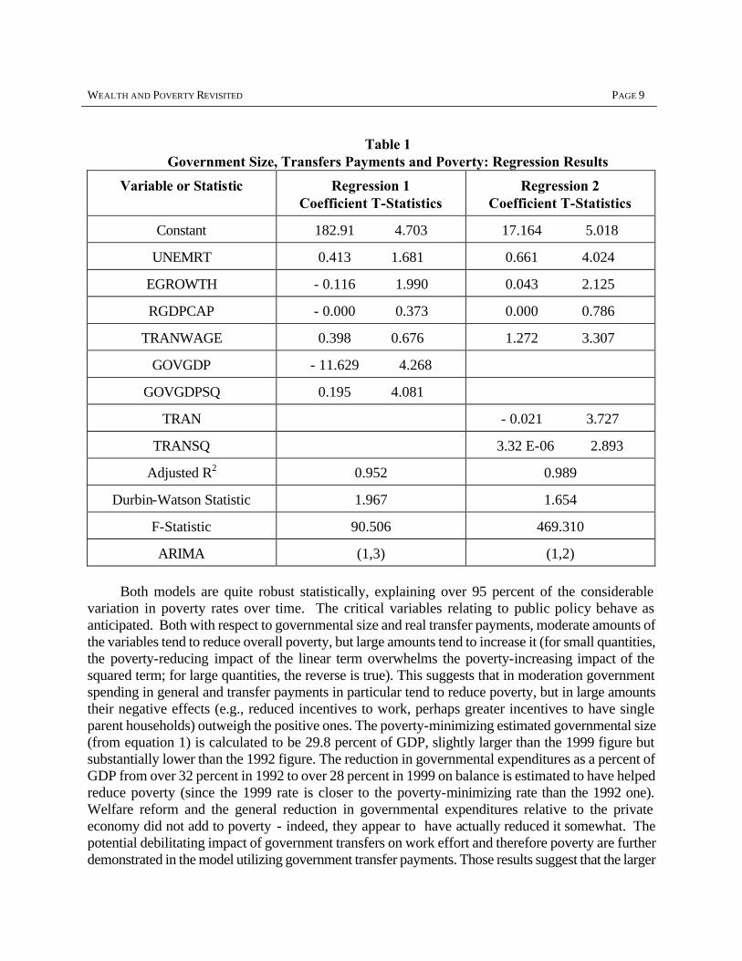
In Table 1, we use ordinary least squares regression analysis to try to explain variations in the

aggregate poverty rate from 1953 through 1999. In the first regression, we used governmental expenditures as a percent of GDP (GOVGDP) and the square of that term (GOVGDPSQ) as measures of governmental size. We also used the ratio of average governmental transfer payments to the average wage (TRANWAGE) as an additional public policy variable. It is expected that modest amounts of government spending would reduce poverty, but that massive spending might lower incentives to work so that GOVGDPSQ might be positive (high spending, higher poverty). To control for business cycles and long-term growth, we introduced three other variables, the unemployment rate (UNEMRT), the growth over the past year in real GDP (EGROWTH), and real gross domestic product per capita (RGDPCAP). In the second regression, we substituted real government transfer payments per capita (TRAN) and the square of that (TRANSQ) for GOVGDP and GOVGDPSQ.


Table 1 Government Size, Transfers Payments and Poverty: Regression Results

Variable or Statistic Regression 1 Coefficient T-Statistics

Regression 2 Coefficient T-Statistics

Constant 182.91 4.703 17.164 5.018

UNEMRT 0.413 1.681 0.661 4.024

EGROWTH - 0.116 1.990 0.043 2.125

RGDPCAP - 0.000 0.373 0.000 0.786

TRANWAGE 0.398 0.676 1.272 3.307

GOVGDP - 11.629 4.268

GOVGDPSQ 0.195 4.081

TRAN - 0.021 3.727

TRANSQ 3.32 E-06 2.893

Adjusted R2 0.952 0.989

Durbin-Watson Statistic 1.967 1.654

F-Statistic 90.506 469.310

ARIMA (1,3) (1,2)

Both models are quite robust statistically, explaining over 95 percent of the considerable

variation in poverty rates over time. The critical variables relating to public policy behave as anticipated. Both with respect to governmental size and real transfer payments, moderate amounts of the variables tend to reduce overall poverty, but large amounts tend to increase it (for small quantities, the poverty-reducing impact of the linear term overwhelms the poverty-increasing impact of the squared term; for large quantities, the reverse is true). This suggests that in moderation government spending in general and transfer payments in particular tend to reduce poverty, but in large amounts their negative effects (e.g., reduced incentives to work, perhaps greater incentives to have single parent households) outweigh the positive ones. The poverty-minimizing estimated governmental size (from equation 1) is calculated to be 29.8 percent of GDP, slightly larger than the 1999 figure but substantially lower than the 1992 figure. The reduction in governmental expenditures as a percent of GDP from over 32 percent in 1992 to over 28 percent in 1999 on balance is estimated to have helped reduce poverty (since the 1999 rate is closer to the poverty-minimizing rate than the 1992 one). Welfare reform and the general reduction in governmental expenditures relative to the private economy did not add to poverty - indeed, they appear to have actually reduced it somewhat. The potential debilitating impact of government transfers on work effort and therefore poverty are further demonstrated in the model utilizing government transfer payments. Those results suggest that the larger


transfer payments are relative to the average wage, the higher the poverty rate is, suggesting large transfer payments lead to a substitution of leisure for work, with a corresponding reduction in income (and increased poverty).

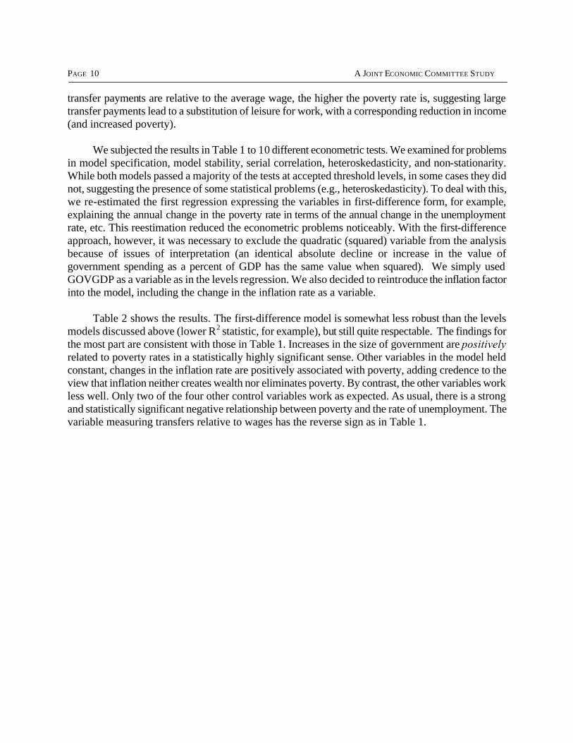
We subjected the results in Table 1 to 10 different econometric tests. We examined for problems

in model specification, model stability, serial correlation, heteroskedasticity, and non-stationarity. While both models passed a majority of the tests at accepted threshold levels, in some cases they did not, suggesting the presence of some statistical problems (e.g., heteroskedasticity). To deal with this, we re-estimated the first regression expressing the variables in first-difference form, for example, explaining the annual change in the poverty rate in terms of the annual change in the unemployment rate, etc. This reestimation reduced the econometric problems noticeably. With the first-difference approach, however, it was necessary to exclude the quadratic (squared) variable from the analysis because of issues of interpretation (an identical absolute decline or increase in the value of government spending as a percent of GDP has the same value when squared). We simply used GOVGDP as a variable as in the levels regression. We also decided to reintroduce the inflation factor into the model, including the change in the inflation rate as a variable.

Table 2 shows the results. The first-difference model is somewhat less robust than the levels

models discussed above (lower R2 statistic, for example), but still quite respectable. The findings for the most part are consistent with those in Table 1. Increases in the size of government are positively related to poverty rates in a statistically highly significant sense. Other variables in the model held constant, changes in the inflation rate are positively associated with poverty, adding credence to the view that inflation neither creates wealth nor eliminates poverty. By contrast, the other variables work less well. Only two of the four other control variables work as expected. As usual, there is a strong and statistically significant negative relationship between poverty and the rate of unemployment. The variable measuring transfers relative to wages has the reverse sign as in Table 1.


Table 2 Determinants of Changes in the Poverty Rate, 1953-98: Regression Results

Variable or Statistic Regression Coefficient T-Statistic

Constant term - 5.293 8.252

Change, Unemployment Rate 0.643 3.497

Change, Real GDP Growth 0.089 1.800

Change, Real GDP Per Capita - 0.001 2.558

Government Spending as % of GDP 0.210 7.486

Change, Transfer Payments as % of Average Wages - 1.356 3.376

Change, % Change, CPI 0.145 2.098

Adjusted R2 0.654

Durbin-Watson Statistic 1.838

ARIMA (0,1)

To further explore the relationship between governmental size, transfer payments and poverty,

we examined some 24 different poverty rates other than the official aggregate rate. We looked at poverty defined by some 11 demographic or social characteristics: poverty of whites, blacks, Hispanics, males, females, full-time workers, families, female-headed families, and persons over 65, under 18, and of working age (18 to 64). We looked at seven different estimates of poverty by location: rural, suburban and central city poverty, and poverty for the four broad Census regions: Northeast, Midwest, South, and West. Finally, we looked at six different definitions of poverty: 125, 150, and 75 percent of the income threshold for the official government poverty definition, definition 15 of the Bureau of Census (producing a low poverty rate because it includes many things in income excluded in the official definition), definition 5 of the Census Bureau (producing a high poverty rate because it excludes some income included in the official definition), and poverty rates calculated using the CPI-U-X1 price index.


Table 3 Summary of 48 Regressions Explaining Poverty Rates in the U.S.

Variable Expected Sign? Significant at 5% Level?

Unemployment Rate 94% 52%

% Real GDP Growth 35 8

Real GDP Per Capita 29 8

Government Spending/GDP 71 38

Gov. Spend/GDP Squared 75 33

Real Tran.Payments/Capita 96 88

Transfer Payments Squared 88 46

% Change, CPI-U 42 2

Transfers As % of Ave.Wage 81 38

Table 3 summarizes the results. We ran 48 regressions, two for each poverty rate. One of those

two regressions used the government size quadratic variables described earlier, while the other used the two transfer payment quadratic variables described above. In general, the results are consistent with earlier findings. The poverty/government spending and poverty-welfare curves were observed in a large majority of regressions, although some of the terms making up the quadratic were statistically significant at the five percent level in only a large minority of regressions. It should be emphasized that the disaggregated poverty rate data are more subject to sampling errors owing to smaller size, and random “noise” in the reported poverty rates makes it more difficult to observe statistically significant relationships with poverty than is the case in the aggregate poverty regressions based on the complete Current Population Survey of typically close to 60,000 households.

While a detailed reporting of the various regressions probably would represent econometric

overkill, below we report the results for one key poverty rate, namely that of people working full-time year-round (WORKPOV) - the working poor. We dropped one control variable that worked the least well (real GDP per capita) in the above table:

(5) WORKPOV = 6.542 + 0.187 UNEM + 0.038 EGROWTH - 0.010 TRAN

(14.247) (4.786) (1.536) (9.024)

+ 1.51E-06 TRANSQ - 0.019 CHCPI + 0.660 TRANWAGE, (4.446) (0.944) (3.758)

_ R2 = .854, F-Statistic = 32.203, ARIMA (0,0),


where CHCPI is the annual percent increase in the CPI, and other variables retain their meaning from Table 1. The model suggests four statistically significant (at the one percent level) determinants of poverty: the unemployment rate, transfers, transfers squared, and transfers as a percent of the average wage. The three transfer variables all work as expected and are robust, as is the unemployment variable. On balance large income transfers are poverty-enhancing, not reducing.10 As indicated above, there is a very strong negative relationship between work effort and poverty.

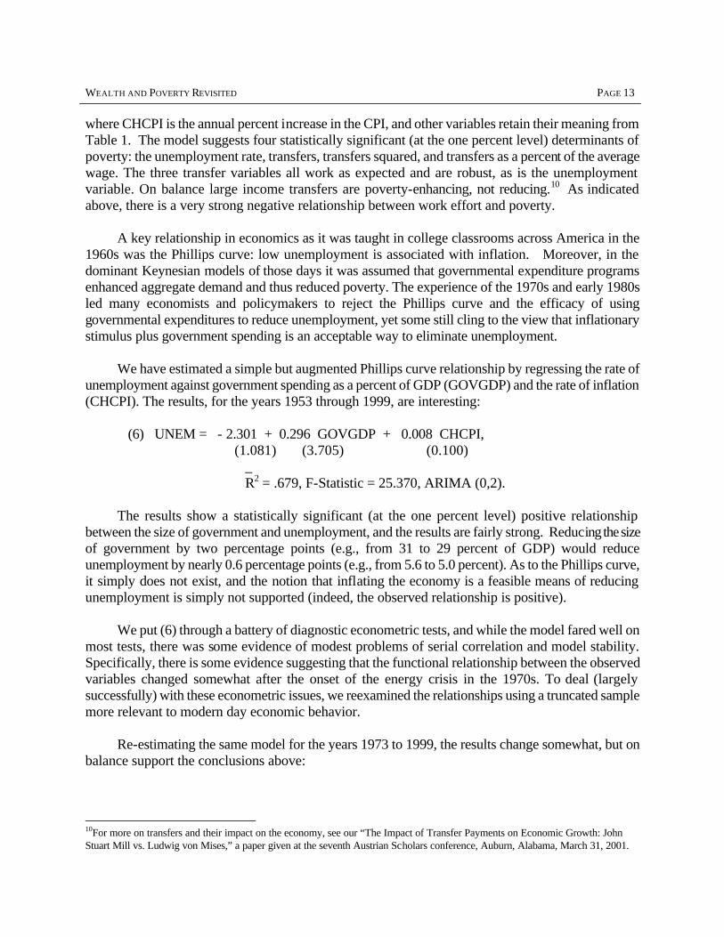
A key relationship in economics as it was taught in college classrooms across America in the

1960s was the Phillips curve: low unemployment is associated with inflation. Moreover, in the dominant Keynesian models of those days it was assumed that governmental expenditure programs enhanced aggregate demand and thus reduced poverty. The experience of the 1970s and early 1980s led many economists and policymakers to reject the Phillips curve and the efficacy of using governmental expenditures to reduce unemployment, yet some still cling to the view that inflationary stimulus plus government spending is an acceptable way to eliminate unemployment.

We have estimated a simple but augmented Phillips curve relationship by regressing the rate of

unemployment against government spending as a percent of GDP (GOVGDP) and the rate of inflation (CHCPI). The results, for the years 1953 through 1999, are interesting:

(6) UNEM = - 2.301 + 0.296 GOVGDP + 0.008 CHCPI,

(1.081) (3.705) (0.100) _

R2 = .679, F-Statistic = 25.370, ARIMA (0,2). The results show a statistically significant (at the one percent level) positive relationship

between the size of government and unemployment, and the results are fairly strong. Reducing the size of government by two percentage points (e.g., from 31 to 29 percent of GDP) would reduce unemployment by nearly 0.6 percentage points (e.g., from 5.6 to 5.0 percent). As to the Phillips curve, it simply does not exist, and the notion that inflating the economy is a feasible means of reducing unemployment is simply not supported (indeed, the observed relationship is positive).

We put (6) through a battery of diagnostic econometric tests, and while the model fared well on

most tests, there was some evidence of modest problems of serial correlation and model stability. Specifically, there is some evidence suggesting that the functional relationship between the observed variables changed somewhat after the onset of the energy crisis in the 1970s. To deal (largely successfully) with these econometric issues, we reexamined the relationships using a truncated sample more relevant to modern day economic behavior.

Re-estimating the same model for the years 1973 to 1999, the results change somewhat, but on

balance support the conclusions above:

10For more on transfers and their impact on the economy, see our “The Impact of Transfer Payments on Economic Growth: John Stuart Mill vs. Ludwig von Mises,” a paper given at the seventh Austrian Scholars conference, Auburn, Alabama, March 31, 2001.


(7) UNEM = - 22.677 + 0.961 GOVGDP - 0.092 CHCPI, (6.351) (11.236) (2.310)

_ R2 = .919, F-Statistic - 83.743, ARIMA (1,1). The relationship between government size and unemployment has actually strengthened

substantially. The model suggests that unemployment rates fall nearly one full percentage point for each one percentage point reduction in government size as a percent of GDP. The relationship is extraordinarily robust, with a double-digit t-statistic. Phillips curves devotees might cheer that the conventional Phillips curve relationship is confirmed at the five percent level of significance. Yet an examination of the coefficient on CHCPI suggests that even if the short-term Phillips relationship exists, it is quite weak. While it would take about a 1.04 percent point reduction in government size relative to GDP to lower the unemployment rate by one percentage point, it would take nearly an 11 percentage point annual increase in the inflation rate to achieve the same effect. Moreover, theoretical advances in economics along with extensive empirical examination suggest that changing expectations work to make the unemployment decline from inflation to be temporary, whereas a decline in governmental size relative to GDP are more likely to improve the operation of labor markets in a manner consistent with a reduction in the “natural rate” of unemployment - that rate of unemployment that is sustainable with price stability. It should be noted that estimating variations of (7) that are not reported here led to consistently powerful and statistically significant relationships between GOVGDP and unemployment, whereas the CHCPI and unemployment relationship observed was often not statistically significant at conventional levels of confidence.11 If the downward Phillips curve exists at all, a dubious proposition based on the mixed evidence, it appears to be very weak and its impact is temporary.

THE KEY TO INCOME AND WEALTH GROWTH: PRODUCTIVITY ADVANCE For the wealth and income of nations to grow on a sustained basis over time, there needs to be an

increase in the output that each worker produces.12 Economic growth and productivity advance are closely and intimately related. Yet the evidence is very clear that large government and inflationary pressures can slow productivity advance. Excessive government lowers the return to private investment (e.g., from the taxes needed to finance government, or from high interest rates arising from deficit-financed government expenditure), reducing capital formation and technological advances that are incorporated in new machines and tools. Inflation distorts the price signals that are key in efficient resource allocation, and increases investment uncertainty; both factors can lower productivity growth.

11 For example, in one estimation, we ran a logarithmic version of (7), with all variables expressed in logarithms. The estimated elasticity of unemployment with respect to government spending as a percent of GDP was a very high 3.97, with a double-digit t-statistic. By contrast, the relationship between the log of inflation and the log of unemployment, while negative, was statistically insignificant at even the 10 percent level. The overall explanatory power of the model was higher than that reported in (7). 12 It is possible for nations to have short-term advances in output per capita without productivity advances, for example by improvements in the terms of trade (e.g., export prices rising relative to import prices), or by increases in the employment-population ratio and/or average hours worked per year. These variables, however, cannot change in a favorable direction indefinitely.


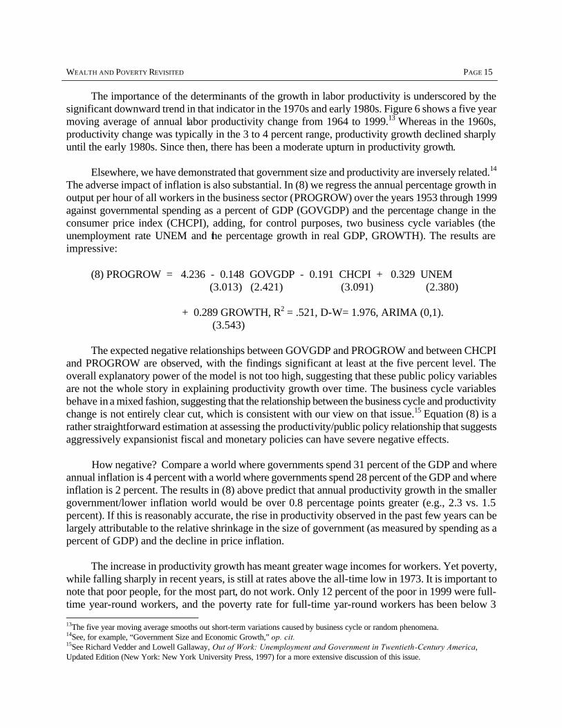
The importance of the determinants of the growth in labor productivity is underscored by the

significant downward trend in that indicator in the 1970s and early 1980s. Figure 6 shows a five year moving average of annual labor productivity change from 1964 to 1999.13 Whereas in the 1960s, productivity change was typically in the 3 to 4 percent range, productivity growth declined sharply until the early 1980s. Since then, there has been a moderate upturn in productivity growth.

Elsewhere, we have demonstrated that government size and productivity are inversely related.14

The adverse impact of inflation is also substantial. In (8) we regress the annual percentage growth in output per hour of all workers in the business sector (PROGROW) over the years 1953 through 1999 against governmental spending as a percent of GDP (GOVGDP) and the percentage change in the consumer price index (CHCPI), adding, for control purposes, two business cycle variables (the unemployment rate UNEM and the percentage growth in real GDP, GROWTH). The results are impressive:

(8) PROGROW = 4.236 - 0.148 GOVGDP - 0.191 CHCPI + 0.329 UNEM (3.013) (2.421) (3.091) (2.380) + 0.289 GROWTH, R2 = .521, D-W= 1.976, ARIMA (0,1). (3.543) The expected negative relationships between GOVGDP and PROGROW and between CHCPI

and PROGROW are observed, with the findings significant at least at the five percent level. The overall explanatory power of the model is not too high, suggesting that these public policy variables are not the whole story in explaining productivity growth over time. The business cycle variables behave in a mixed fashion, suggesting that the relationship between the business cycle and productivity change is not entirely clear cut, which is consistent with our view on that issue.15 Equation (8) is a rather straightforward estimation at assessing the productivity/public policy relationship that suggests aggressively expansionist fiscal and monetary policies can have severe negative effects.

How negative? Compare a world where governments spend 31 percent of the GDP and where

annual inflation is 4 percent with a world where governments spend 28 percent of the GDP and where inflation is 2 percent. The results in (8) above predict that annual productivity growth in the smaller government/lower inflation world would be over 0.8 percentage points greater (e.g., 2.3 vs. 1.5 percent). If this is reasonably accurate, the rise in productivity observed in the past few years can be largely attributable to the relative shrinkage in the size of government (as measured by spending as a percent of GDP) and the decline in price inflation.

The increase in productivity growth has meant greater wage incomes for workers. Yet poverty,

while falling sharply in recent years, is still at rates above the all-time low in 1973. It is important to note that poor people, for the most part, do not work. Only 12 percent of the poor in 1999 were full-time year-round workers, and the poverty rate for full-time yar-round workers has been below 3 13The five year moving average smooths out short-term variations caused by business cycle or random phenomena. 14See, for example, “Government Size and Economic Growth,” op. cit. 15See Richard Vedder and Lowell Gallaway, Out of Work: Unemployment and Government in Twentieth-Century America, Updated Edition (New York: New York University Press, 1997) for a more extensive discussion of this issue.


percent for every year since 1984.16 Productivity advances lift workers out of poverty, but do little to help those not working. The poverty problem thus is largely a problem of employment, not one of inadequate wages, etc.

SOME IMPLICATIONS FOR PUBLIC POLICY While money alone cannot buy happiness, the acquisition of income and wealth contributes to the

well-being of individuals. Given a choice of having a lot of wealth or a little, most people would prefer a lot. The popularity of the television show Who Wants to Be a Millionaire? reflects the human yearning for material affluence. Other things equal, then, public policy should enhance economic growth and promote, not inhibit, the creation of wealth. Similarly, poverty (a lack of income) is a condition that few persons enjoy, and the eradication of poverty is obviously a public goal.

Government can sometimes help in both the creation of income and wealth on the one hand, and

the eradication of poverty on the other. In a world without governmental involvement, the provision of some modest amounts of public assistance for people temporarily destitute would no doubt reduce poverty. In societies with virtually no public services, increases in governmental expenditures to protect property rights, provide for a rule of law, and perhaps provide basic infrastructure will increase income and wealth.17 Government can thus sometimes be a positive force in economic development and poverty eradication.

Having said that, there is strong evidence that much modern public policy to enhance wealth and

eradicate poverty has been self-defeating. Other things equal, increases in governmental spending relative to GDP tend to reduce wealth and income growth in modern American society, and even more so in the welfare states of modern Europe. The moderation that Aristotle called for in human affairs applies to governmental fiscal policy as well. The Aristotelian “golden mean” can literally bring gold - wealth - to nations if practiced with respect to governmental expenditure.

The 1990s were a decade of prosperity to a considerable extent precisely because governmental

spending as a percent of GDP fell. From our statistical estimation above, we would estimate that the net worth of Americans per capita in 1999 would have been nearly $5,000 lower had their been no decline in government spending as a percent of GDP after 1992. Similarly, that moderation in government spending also lowered, not raised, the rate of poverty.

The evidence is moderately strong that for most subsets of the population, governmental activity

reduces poverty when that activity is undertaken in moderation, but increases poverty when spending passes a threshold where the behavioral attributes associated with higher government spending actually increase poverty. Those attributes include reduced work effort and living outside of

16On poverty data, see U.S. Bureau of the Census, Current Population Reports P60-210, Poverty in the United States:1999 (Washington, D.C.: U.S. Government Printing Office, September 2000). Also, see our “The Minimum Wage and Poverty for Full-Time Workers,” Journal of Labor Research, forthcoming. The addition of a minimum wage variable to poverty regressions changes things little, since there is little association between minimum wages and poverty rates. 17See the JEC studies on government size and economic growth by us and by Gwartney, Lawson and Holcombe, op. cit.


traditional marital arrangements. The evidence is even stronger specifically with respect to government spending on transfers, where the evidence of the poverty-welfare curve remains strong.18

Two other variables conform with expectations in a large majority of the regressions discussed

here: the unemployment rate and transfers as a percent of average wages. The evidence is very strong that unemployment creates poverty, and nearly as strong that when government transfer payments become high in relation to wages, the substitution of transfers (e.g., welfare payments) for work leads in some cases to poverty.

Current Policy Initiatives

A major initiative of the new administration is to reduce taxes, particularly on income (especially individual income taxes) and wealth (especially death duties). While the regressions above did not explicitly look at taxes, the correlation between taxes and government expenditures is extremely high. Moreover, numerous other studies confirm that there is an inverse relationship between taxes and economic growth.19 Beyond that, however, the political economy of policy making suggests that a tax cut could have favorable implications for growth. In a much publicized study, we once argued that when tax revenues increase by one dollar, expenditures rise by $1.59. The same principle applies in reverse, although the number may not be precisely $1.59. In other words, reduced budget surpluses will increase the political costs to Members of Congress of increasing government spending faster than inflation.

Moreover, evidence from the postwar era is that budget surpluses tend to be dissipated if they

accumulate for long, with 60 cents of each dollar being spent within a year.20 The historical evidence affirms that lower tax revenues reduce the ability or the political desire of Congress and the Administration to engage in expansionary spending programs. Other things equal, a tax reduction is likely to reduce governmental expenditure.

Moreover, the results here and by other researchers suggest that the economic growth effects of

lower marginal rates of taxation and smaller governmental expenditure are positive, increasing tax revenues more than what relatively static estimates of the Congressional Budget Office or Joint Tax Committee would suggest. Our findings are broadly consistent of those of Martin Feldstein and associates at the National Bureau of Economic Research that suggest that the revenue loss from the Bush tax proposal is likely to be much smaller than officially estimated.

18 An early, but exhaustive empirical demonstration of the existence of the poverty-welfare relationship can be found in our monograph, Poverty, Income Distribution, the Family and Public Policy, study, Joint Economic Committee (Washington, D.C.: Government Printing Office, 1986). 19An early JEC study is Richard K. Vedder, “State and Local Taxes and Economic Development: A Supply-Side Perspective,” (Washington, D.C.: Government Printing Office, 1981). An update of that study published by the JEC is “State and Local Taxes and Economic Growth: Lessons for Federal Tax Reform,” December 1995. Two representative studies reaching simila r conclusions are Alaeddin Mofidi and Joe A. Stone, “Do State and Local Taxes Affect Economic Growth?” Review of Economics and Statistics, November 1990, and Paul Cashin, “Government Spending, Taxes, and Economic Growth,” International Monetary Fund Staff Papers, June 1995. 20See Richard Vedder, Lowell Gallaway and Christopher Frenze, “Taxes and Deficits: New Evidence (“The $1.59 Study”), Joint Economic Committee Study, October 30, 1991; see also Richard Vedder and Lowell Gallaway, “Budget Surpluses, Deficits and Government Spending,” Joint Economic Committee Study, December 1998.


One reason that tax reductions stimulate economic activity is that taxation inevitably imposes

what economists call “deadweight losses” on the population. For example, consumption taxes raise the retail prices of goods, leading to reduced trade and a loss of consumer welfare. Economist call the gains that consumers receive from being able to buy most goods for less than they would have been willing to pay “consumer’s surplus.” If prices rise because of tax increases, those gains decline, and they are only partly offset by the welfare gains associated with tax revenues. Hence the term “deadweight losses.”

The extent to which taxes impose deadweight losses is debatable, but is nearly universally

acknowledged to be sizable. While the pioneering study by Arnold Harberger on this topic found deadweight losses to be around five percent of revenues, studies by Stuart and by Ballard, Shoven and Whalley put them much higher - at least 15 percent of revenues and possibly 50 percent or more.21 The midpoint of the Ballard, Shoven and Whalley estimates is 33 cents. Stuart puts the loss at somewhat over 50 cents. The midpoint of this range of estimates (30 to 50 cents per dollar) is 40 cents. To be sure there are still higher estimates (some of Browning's, Feldstein's), as well as lower ones (e.g., the original Harberger, Goolsbee), but the 40 cent estimate is probably approximately a midpoint estimate of the many serious studies performed. The 1993 increase in the federal income tax had particularly debilitating deadweight loss effects in the highest marginal tax brackets according to Martin Feldstein of Harvard University and the National Bureau of Economic Research, and associates. They estimated that the repeal of $8 billion in taxes on high income individuals would reduce deadweight losses by $24 billion annually - 300 percent!22 This is particularly relevant to current discussions, as President Bush’s tax proposal calls for essentially repealing the 1993 increases in the highest marginal rates as part of a comprehensive rate reduction program.23

Another current argument for tax reduction relates to the current softness in the economy. While

we believe that demand-side macroeconomic stimulus has little or no positive effect on long term economic growth, the proposed supply-side tax cut may nonetheless have some secondary benefits by providing some demand stimulus which could mitigate the current slowdown in GDP growth if it is promptly forthcoming. As the regressions above indicated, high unemployment tends to lead to wealth reduction and poverty increases. To the extent that tax reduction on incomes similar to that proposed by President Bush prevents increases in unemployment, it should reduce the probability of reductions in income and wealth, and the associated increase in the rate of poverty.

One objection to large tax reductions is that somehow this will endanger our ability to meet

Social Security obligations. While this paper is not the place to engage in a detailed discussion of the

21Arnold Harberger, “Taxation, Resource Allocation, and Welfare,” in John Due, ed., The Role of Direct and Indirect Taxes in the Federal Revenue System (Princeton, NJ: Princeton University Press, 1964); Charles Stuart, “Welfare Costs per Dollar of Additional Tax Revenue in the United States” American Economic Review, June 1984; Charles J. Ballard, John Shoven, and J. Whalley, “General Equilibrium Computations of the Marginal Welfare Costs of Taxation in the United States,” American Economic Review, March 1985. 22Martin Feldstein and Daniel Feenberg, “The Effect of Increased Tax Rates on Taxable Income and Economic Efficiency: A Preliminary Analysis of the 1993 Tax Rate Increase,” in Jomes Poterba, ed., Tax Policy and the Economy (Cambridge, MA: MIT Press, 1996); Feldstein, “Tax Avoidance and the Deadweight Loss of the Income Tax,” Cambridge MA: NBER Working Paper W5055, March 1995, and his “How Big Should Government Be?” NBER Working Paper W868, December 1996. 23For a somewhat more extended discussion of the deadweight loss issue with additional references, see our JEC study, “Tax Reduction and Economic Welfare,” April 1999, available at http://www.house.gov/jec/fiscal/tax/reduce.htm.


accounting dimensions of Social Security, the need for or feasibility of a “lockbox” to protect funds, etc., the results above suggest one thing: the higher economic growth likely to result from tax reductions increases the ability of future working age Americans to meet their obligations to the elderly or disabled. If the economic pie gets larger, it becomes less burdensome to offer a given sized piece of that pie to our senior citizens.

An example will illustrate that point. For the sake of simplicity, assume that current output is

equal to 100, that 15 percent (15 units) of that goes for investment, and the remainder (85) for consumption (some of that financed by government). Let us assume of the 85 units for consumption that 75 go for the working age population and their children, and the other 10 go to retirees. For the sake of simplicity, assume all retiree income is financed by Social Security.

Assume that over time that the desire is to provide constant real income per capita for retirees,

and also that the number of retirees is going to grow in a relative as well as an absolute sense as the population ages and medical advances continue. Suppose it will take 20 units of output to finance the consumption of the retirees in 2021, 20 years from now (implying a growth in real obligations of 3.6 percent a year). Suppose that we maintain governmental expenditures at existing levels relative to GDP, have moderate inflation, and have 3 percent annual growth in GDP over the next 20 years. Output will rise to 180.6 by 2021 years (reflecting 3 percent output growth compounded annually for 20 years). With Social Security obligations doubling but output growing only 80 percent, the retirement/Social Security burden will rise from 10 to 11 percent of GDP. Whereas at the present, Social Security obligations are covered by current Social Security taxes, that would possibly not be the case in 20 years under this scenario. In any case, with rising Social Security obligations relative to GDP, at some future date there would be deficits in the Social Security accounts that would exhaust the Social Security Trust Fund.

Suppose that tax reductions prompt some decline in expenditures relative to GDP, and that

monetary policy moves to promote complete price stability. Our regressions above would suggest annual GDP growth would rise, quite plausibly to 3.6 percent. In that case, output will double to 200 in 20 years, and there will be no increase in Social Security’s share of output (20 is still 10 percent of 200), and existing taxes would likely continue to more than cover current obligations. The problem of financing Social Security pensions would be dramatically alleviated.

It is true that current Social Security law adjusts pensions upward with rising real wages, and

that higher economic growth would mean higher real wages and thus pension obligations. If a funding problem looms in the future under a higher economic growth scenario, it reflects a decision to increase real pension benefits of future retirees over current levels. The basic principle that economic growth lowers the burden of any given sized future obligation still holds. A richer nation can do more things.

With respect to poverty, it is worth noting that through most of our modern economic history,

poverty reduction followed from economic growth. The one exception was the era of the 1970s through the early 1990s, when an excessively generous welfare state undermined the sense of individual responsibility and self-help among many of our nation’s poor. The reduction in poverty the last several years will likely continue in the future if the rewards to work continue to increasingly outdistance the rewards of not working in the form of public assistance. Welfare reform in the mid-


1990s was a step in insuring that the eradication of poverty through economic growth will continue in America.

AN EPILOGUE: NEW DATA SHOWING DECLINING WEALTH Since the completion of research for this paper, the Federal Reserve System has released data

for the year 2000 suggesting that household net wealth declined by about two percent from 1999, and by well over five percent on a real per capita basis. This reverses the sharp upward trend shown in Figure 1. Is this wealth decline inconsistent with the earlier discussion? The answer is clearly “no.”

The model discussed in this paper suggested that wealth varies inversely with the growth in

governmental expenditures and the rate of inflation. In the past year, there has been a sharp increase in planned governmental expenditures as a consequence of legislation passed by the Congress and signed by former President Clinton. Because of the lag between legislative action and spending activity, the election year spending spree has not yet shown up yet in a major increase in spending, but there is a widespread anticipation that that will happen. Investors, seeing the possibility of increased crowding out of private sector activity, may have become more wary of purchasing securities and other forms of wealth. The concerns of Federal Reserve Chairman Greenspan and others during the first half of 2000 about potentially renewed inflationary threats, heightened by sharply rising energy prices, also probably contributed to investor wariness. While other factors (e.g., the possibility of a business cycle decline) no doubt also play a role, the rising probability of a rise in the growth of government spending and prices has no doubt contributed to recent market declines and a falling in real personal wealth.

If anything, the decline in wealth in 2000 increases the case for a tax cut. As part of his proposed

budget for fiscal year 2002, President Bush has proposed keeping expenditure growth below the anticipated growth in national output, which should enhance private sector initiatives and the creation of wealth, and offsetting the negative effects of the spending initiatives approved in 2000.

CONCLUSIONS There are compelling arguments for promoting moderation in the growth of governmental

expenditures over time. A potentially politically viable policy for promoting economic growth would be to allow government expenditures to rise modestly over time, but by less than the growth rate in GDP, leading in time to some reduction in governmental expenditures as a percent of GDP. In effect, this has been the experience of the past several years. The benefits of moderating inflation observed in recent times are arguments for the Federal Reserve continuing to follow its stated objective of promoting price stability. Since taxes tend to automatically rise over time as a percent of GDP (in large part, because of the progressive nature of the income tax), and since tax reduction also tends to reduce the propensity of policy-makers to increase expenditure, a very strong case can be made for a tax cut. Current softness in the economy further supports the case for tax reduction.

wealth and poverty revisited - senate

Documents