Sef Meens Eriksson

Spring semester 2017

Bachelor level, 15 ECTS

Politices Bachelor Program

Wealth inequality and

redistribution

Possibilities of redistributive policies with an application to

Sweden, Germany and the UK.

Sef Meens Eriksson

Abstract

The aim of the study is to answer what governments can do to work against increasing wealth

and income inequalities. In a theoretical part I describe how inheritance and income inequality

are important driving factors to wealth inequality and the potential role of the government to

counteract increasing monetary inequalities. The empirical part narrows the scope to income

inequalities and how the governments of Sweden, Germany and the UK have conducted their

redistribution policies between the 80’s and the mid 00’s. The most interesting results from

the empirical part indicate that income inequalities before any income redistribution has risen

in all three countries, income inequality after income redistribution has also risen but not as

much. The UK clearly is the country which redistribute the least and in addition has the

greatest post redistribution income inequality, much greater than both Sweden and Germany

which redistribute about as much of income. Further, it is shown that poor citizens in all three

countries in all years gain relatively more (net gain of redistribution as share of an

individuals’ total income) than wealthy from the redistribution scheme. Due to lack of wealth

data the empirical calculations were based on capital income as a proxy for wealth.

Table of contents

Abstract ...................................................................................................................................... 2

Table of figures .......................................................................................................................... 5

Introduction ................................................................................................................................ 1

Part 1 .......................................................................................................................................... 2

1.1 Research question ............................................................................................................. 2

1.2 Structure of the study ....................................................................................................... 3

1.3 Wealth inequality problematized ..................................................................................... 3

1.3.1 Preferences for income and wealth ........................................................................... 3

1.3.2 Social inheritance ...................................................................................................... 4

1.3.3 Inequality as harmful to society? .............................................................................. 4

1.4 Channels for intergenerational transmission .................................................................... 5

1.4.1 Inheritance ................................................................................................................. 5

1.4.2 Education and health care system ............................................................................. 6

1.4.3 Factors on the macro level......................................................................................... 6

1.5 Role of the government .................................................................................................... 7

1.5.1 Education and health care systems ............................................................................ 8

1.5.2 Taxing unfair wealth inequality ................................................................................ 8

1.6 Income redistribution as a policy tool .............................................................................. 9

1.6.1 Economic arguments ............................................................................................... 10

Part 2 ........................................................................................................................................ 10

2.1 Data ................................................................................................................................ 10

2.2 Method ........................................................................................................................... 11

2.2.1 Selection of variables .............................................................................................. 11

2.2.2 Missing values, top and bottom coding ................................................................... 12

2.2.3 Equivalence scales & weights ................................................................................. 13

2.2.4 The Lorenz curve .................................................................................................... 13

2.2.5 The Gini coefficient ................................................................................................ 15

2.2.6 Redistribution relevance for poor respective wealthy ............................................. 16

2.2.7 Limitation of the study ............................................................................................ 16

Part 3 ........................................................................................................................................ 18

3.1 Empirical results ................................................................................................................. 18

3.1.1 Gini coefficients ...................................................................................................... 18

3.1.2 Lorenz curves .......................................................................................................... 20

3.1.3 Relevance of redistribution for wealthy respective poor......................................... 26

Part 4 ........................................................................................................................................ 30

4.1 Discussion ...................................................................................................................... 30

4.2 Concluding remarks ....................................................................................................... 33

Reference list ............................................................................................................................ 34

Journal papers ....................................................................................................................... 34

Books .................................................................................................................................... 35

Websites ............................................................................................................................... 35

Appendix 1 ............................................................................................................................... 36

Appendix 2 ............................................................................................................................... 37

Table of Lorenz curves for Sweden ..................................................................................... 37

Pre redistribution .............................................................................................................. 37

Post redistribution ............................................................................................................ 38

Table of Lorenz curves for Germany ................................................................................... 40

Pre redistribution .............................................................................................................. 40

Post redistribution ............................................................................................................ 41

Table of Lorenz curves for the UK ...................................................................................... 43

Pre redistribution .............................................................................................................. 43

Post redistribution ............................................................................................................ 44

Table of figures

Figure 1, Basic Lorenz curve, reproduced from Ray (1998, pp. 178-184) .............................. 14

Figure 2, Graphic derivation of the Gini coefficient ............................................................... 15

Figure 3, Different Lorenz but the same Gini .......................................................................... 16

Figure 4, Pre and post Gini coefficients ................................................................................... 19

Figure 5, Pre redistribution Lorenz curves, Sweden ................................................................ 21

Figure 6, Post redistribution Lorenz curves, Sweden ............................................................... 21

Figure 7, Overview table of redistribution trends, Sweden ...................................................... 22

Figure 8, Pre redistribution Lorenz curves, the UK ................................................................. 23

Figure 9, Post redistribution Lorenz curves, the UK ................................................................ 23

Figure 10, Overview table on redistribution trends, the UK .................................................... 24

Figure 11, Pre redistribution Lorenz curves, Germany ............................................................ 25

Figure 12, Post redistributioin Lorenz curces, Germany ......................................................... 25

Figure 13, Overview table on redistribution trends, Germany ................................................. 26

Figure 14, Redistribution relevance along the capital income distribution, Sweden ............... 27

Figure 15, Redistribution relevance along the capital income distribution, Germany ............. 28

Figure 16, Redistribution relevance along the capital income distribution, the UK ................ 29

1

Introduction

The distribution of wealth has varied a lot over time but also between countries, still the

trends have been similar in most advanced western economies during the last 150 years. The

19th century was characterized by great wealth inequalities where small groups advantaged

extremely by the industrial revolution. This concentration of wealth declined significantly as a

result of the two world wars which destroyed capital but also brought about high taxes

targeted on the wealthy in order to fund the wars (Piketty and Saez, 2014; Saez and Zucman,

2016). In the time after the Second World War, especially since the 70’s, wealth concentration

once again increased which is a development recognized and perceived as problematic by

both academics and policy institutions like the World Bank and the OECD (Förster and delle

Politiche Sociali, 2011; “Poverty and Shared Prosperity 2016,” n.d.).

This concentration of wealth must be perceived and interpreted in the context of other societal

developments as well as a phenomenon interconnected to wealth concentration in previous

periods. Moreover, a dimension and understanding of fairness should be applied when wealth

inequalities are to be analyzed. One cannot ignore that people do not share equal preferences

for wealth, hence there will be wealth inequalities around which must be considered as fair.

The unfair inequality on the other hand stems from factors beyond reach of individuals. Most

important is the existence of inheritance, both monetary and social, and how it positions

children with unequal opportunities to prosper in an economic sense. There are several ways a

society can correct for wealth inequality which is not related to variation in individuals’

efforts, how these potential policy tools are used varies between countries. What all countries

share though, is some level of preference for income redistribution, but how they are

formulated and acted out into policies varies a lot. In the empirical part of this study I

examine how the governments of Sweden, Germany and the UK in 1979-2005 have used the

policy instrument of income redistribution. This empirical approach will give a deepened

understanding of one of many policy tools that are used to counteract increasing wealth and

income inequalities.

I will initiate the study with a broad theoretical perspective on wealth inequality and the major

driving factors and mechanisms that affect wealth inequality. The broader perspective will

successively be narrowed down for the empirical part which focus on income redistribution as

2

a crucial driving factor for wealth inequality. To study wealth and income inequalities is

important due to the broad audience it speaks to. Not only policy makers have an interest in

understanding driving factors and inequality trends but also the broader public, Emmanuel

Saez formulates it neatly; “People have a sense of fairness and have views on whether the

distribution of economic resources is fair” (2017, pp. 8).

Part 1

Wealth inequality does not appear from a blue sky, it is a phenomenon which must be

understood in the context of other societal trends and developments. To start with wealth

inequality of today’s society is an obvious consequence of yesterday’s society due to the

presence of inheritance. Due to the social and legal norms that inheritance comprises do

individuals’ wealth depend on the wealth of other individuals, their parents. Another

important driving factor to wealth inequality is income inequalities since a person with higher

income probably will accumulate more wealth compared to a low-income earner, equal tax

circumstances and preferences assumed. Understanding the close connections between wealth

inequality, income inequality and inheritance inequality is crucial and will also be in the scope

of this study.

1.1 Research question The research question I will try to answer in the study is how can government policies

counteract increasing wealth and income inequality? To start with I will establish a

theoretical perspective on the issue; of why wealth and income inequalities at all should be

cared about and how policy instruments could be used to decrease wealth and income

inequality. Moreover, the empirical part will contribute to the research question by focusing

on trends in income redistribution in three different countries. By narrowing the scope to

income redistribution trends across countries, I will be able to determine whether the

countries have kept income inequalities stable over time, or not. Furthermore, income

redistribution and inequality obviously is interesting when we aim to understand wealth

inequalities, due to the importance of income inequality as a determinant of wealth

inequalities.

The empirical application is conducted on three countries with different characteristics;

Sweden, which is a country perceived to have high monetary equality, the UK with a tradition

3

of great monetary inequality, and Germany which is a country that in many cases has taken a

middle position between the previous two countries. The three countries are studied for the

period of 1979-2005, the limited time studied is due to limitations in the data.

1.2 Structure of the study Onwards Part 1 will unfold as follows; In chapter 1.3 I will discuss fairness of wealth

inequality and potential negative effects of wealth inequality to a society. In Chapter 1.4

drivers to wealth inequality, which are out of reach for the individual, will be described.

Further is chapter 1.5 connecting to chapter 1.4, the role of the government is explained and

how it can use policy implementation to affect wealth inequality. Last in Part 1 (chapter 1.6) I

will narrow the scope to the topic of the empirical application of the study; income

redistribution as a policy tool available for a government. Moreover, I describe the data and

method used in the study in Part 2, also limitations of the study are included here. In Part 3 I

describe the empirical results and last, in Part 4, I will have a discussion and concluding

remarks.

1.3 Wealth inequality problematized

1.3.1 Preferences for income and wealth

Clearly, great wealth inequalities exist in most countries and have been doing so for a long

time, but could these inequalities possibly be considered as fair? To put is simple, is it not fair

that a doctor earns more than a cashier in the local supermarket? With certainty, the doctor

has invested much more time, effort and money in his or her choice of occupation. Hence one

could argue that it is fair by the society to reward such a person which has strong preferences

for income. Whether a person accumulate wealth or not is further dependent on preferences

for saving and consumption. A population with a variety of preferences consequently will

become unequal, both regarding income and wealth, therefore some degree of monetary

inequality should be perceived as fair (Piketty and Saez, 2012). Now add another generation

(equally many people as the previous) to the context where all wealth has been transmitted to

the latter generation through inheritance. The wealth inequality will be the same in the latter

generation as it was in the previous but there is an important difference to have in mind. The

matter of preferences for saving and consumption as a determinant of personal wealth is now

replaced by the factor inheritance, a benefit the inheritor is not responsible for. This simple

4

example reveals that inheritance is problematic from a fairness perspective. Studies also

support this; less acceptance is shown by people towards wealth inequalities when preferences

for wealth or savings are not the underlying factors (Björklund et al., 2012; Piketty and Saez,

2012). This shows that some degree of wealth inequality can be fair, or at least perceived as

far which is of greater relevance for policy makers in the field of redistribution policies.

1.3.2 Social inheritance

The phenomenon of inheritance has a social aspect as well, where preferences for wealth also

are inherited to some extent, this complicates the question about fairness quite a lot which I

will explain in this paragraph. An individual who inherits great ambitions for school results

for instance, is more probable to reach a high paid job. To draw a distinction whether this is

fair or not could be tricky. Other cases where societies actually do correct for inequalities

considering ability to prosper in life, is when individuals are caused by disabilities, mental

retardation or congenital disease etc. Societies perceive such circumstances as random

misfortune and hence should be corrected for (Roemer, 1993), at least to some extent. In

theory, this could be applied to all random misfortunes happening to individuals, but a clear

distinction of random vs non-random factors is difficult. An objective assessment appears to

be difficult and hence is the debate on social inheritance and fairness often driven by

ideological beliefs. Liberal parties emphasize the responsibility of personal choices, and less

the importance of social inheritance. Left-wing parties on the other hand, stresses the

influence of structural forces leading people into different economic positions. No matter

political belief it seems clear that social inheritance exists and that it influences wealth and

income inequality (Björklund et al., 2012, 2012; Black and Devereux, 2010; Bowles and

Gintis, 2002), hence it is important to be aware of.

1.3.3 Inequality as harmful to society?

Beliefs and emphasis on social inheritance apparently constitute political differences, but even

more interesting is how ideas go apart regarding how wealth inequality is harmful to society or

not in a wider perspective (Finnie et al., 2006, pp. 150-151). Some researchers appreciate

inequality as a necessity since it would create economic incentives for people to work harder

which could be desirable for a countries’ economy. The opposite arguments stresses how both

wealth and income inequality is a hotbed for criminality, distrust and an unhealthy societal

climate which neither benefits rich or poor in the long run (Diamond, 2005; Fajnzylber et al.,

5

2002). Another consequence of increased wealth inequality is lower intergeneration mobility

through the income and wealth distribution, i.e. that children of poor parents are less likely to

become wealthy compared to children of wealthy parents. Inheritance is an important factor for

this negative effect since it positions individuals with varying wealth irrespective that

individuals’ preference for wealth (Finnie et al., 2006). Decreasing intergenerational mobility

through the income and wealth distribution will not only concentrate wealth in the upper tail of

the wealth distribution even more, also power will concentrate which adds another dimension

into the discussion of fairness (Glaeser, 2005).

1.4 Channels for intergenerational transmission

In the previous chapter the role of individual preferences, fairness and potential harm to

societies were described. Now I will move away from factors that the individual can affect to

some extent. Instead I will describe three major factors influencing individuals’ equal

opportunity to prosper monetarily in life; inheritance, welfare systems and macro shocks. This

chapter broadens the picture of what really affects wealth inequality and it becomes apparent

that individual preferences cannot be perceived as the sole driving factor of wealth inequality.

1.4.1 Inheritance

While each individual bear at least some responsibility for its occupation this is certainly not

the case when it comes to inheritance (Ohlsson and Nordblom, 2002). Inheritance is an

important channel for intergenerational wealth transmission (Elinder et al., 2016; Piketty and

Zucman, 2014; Saez, 2017) but there are disagreements on how to look upon the

phenomenon. One line of argumentation follow the ideas of Roemer (1993); inheritance is

unfair simply because it gives individuals different endowments which they have not earned

themselves, hence this inequality should be corrected for. The opposite stand is rather liberal

and emphasizes the importance of individual freedom. If parents want to bequest their wealth

to their children nothing must stop them from doing so. What is worth remembering though is

that parents’ taste for bequest is not the single determinant for how much their children will

inherit. Also the parents’ labor income and the inheritance of their parents have an impact on

how large inheritance the children will receive in the end (Piketty and Saez, 2012). To

summarize, it is clear that individuals’ preferences for wealth is only one of many factors

determining the probability of an individual to become wealthy.

6

1.4.2 Education and health care system

Moving beyond individually varying factors like inheritance the importance of educational

structure should be acknowledged and how this certainly has an impact on whether

individuals are offered equal opportunities in life. An educational system with low entry

barriers will naturally decrease future income inequalities since human capital plays an

important role for future income levels (Björklund and Jäntti, 2009) and consequently also the

wealth inequalities. Moreover, the educational system can have a direct redistributive effect,

high income earners contribute more to the welfare system than low income earners through

taxes, still both groups could advantage equally from the educational system. An additional

redistributive effect is reached if wealthy or high earners pay higher fees than poor, less

redistributive effects occur if the subsides are low and uniform for the whole population.

Similar mechanisms for equal opportunities and redistributive effects are relevant for the

health care system.

1.4.3 Factors on the macro level

Both inheritance and welfare systems are issues within reach for legislators to affect, however

that is not true for all macro shocks that certainly also could have an impact on wealth

inequality in a country. In Sweden for instance the financial crisis in 2008 caused a significant

concentration of wealth as a direct consequence of a price boom on the housing market, a

market of assets mainly held by the upper middle class (Lundberg and Waldenström, 2016,

pp. 2–3). Another example is how national financial market can boom; in the 80’s the average

real price on the Stockholm stock market increased by 13% annually and by 16% during the

90’s. The same numbers for the New York stock market was 3 respective 6% (Roine and

Waldenström, 2012). First of all, such a rapid growth of financial values can increase wealth

inequalities within a country, dependent on tax structures, since the wealthier part of

populations normally holds the majority of financial assets. Moreover, this can offer relevant

clues on why wealth inequality within different countries may diverge.

Now let us look beyond shocks caused by financial crises, tax policies or other general

economic fluctuations. Then structural patterns related to net rate of return, population growth

and growth rate of an economy also have an impact on wealth inequality. The period before

the industrial revolution was characterized by growth rates just above zero percent while the

net rate of return was around 5%. This relation led to drastic increases of wealth inequalities

7

in many industrializing countries. According to the same logic did a decreasing gap between

net rate of return and growth rates in the first half of the 20th century serve as a great equalizer

together with the two world wars. Predictions of the century ahead of us suggests that

increased competition for capital will push up net rates of return, in addition projections

indicate that both population growth as well as economic growth rates will decrease.

Following the same logic as previous, this will push for increased wealth inequalities (Piketty

and Zucman, 2014) and probably increase the gap between GDP growth and net rate of return

after taxes. This will constitute a force pushing for increasing wealth inequalities (Piketty and

Zucman, 2014, pp. 842).

In this chapter I have shown that wealth and income inequality in many aspects are beyond

control of individuals and sometimes even beyond control of national legislators. A study by

Emmanuel Saez (2017) confirms this description, at the same time he is really clear on the

relevance of domestic legislation. As an example, he shows that the increase in income

concentration since the 70’s was much lower in France and Sweden compared to the US,

although all three countries have been “subject to the same forces of globalization” (Saez,

2017). The governments seem to, at least to some degree, carry the capacity of determining

the paths of inequality and this is also what will be problematized and described in the

following chapter.

1.5 Role of the government

From the previous chapter, we learned that legislators have power to affect the wealth

inequality, which raises the question on which political path to choose. Hence, the aim of the

government must be defined; to emphasize the freedom of choice for all individuals or to

correct for circumstances which creates unequal possibilities to prosper in life. In this chapter

I will describe possible government actions in accordance with the second approach; to offer

equal opportunities and decrease wealth inequalities derived from factors which cannot be

derived to individual variation in efforts or preferences. Since there are a range of potential

policy tools available to legislators there are as many empirical approaches possible. Due to

the restrictions of this study I will focus the empirical part of the study to one prominent

policy instrument, the income redistribution. But before scrutinizing that further a brief

coverage of the other most important policy tools used will be done.

8

1.5.1 Education and health care systems

Welfare systems are a crucial factor for equal opportunities in a society, though the potential

paths of policies are many. In general, the education systems in Germany and the UK are

leaning more towards a conservative idea that individuals are suited for different professions

and hence should be offered that specific schooling from a young age. Even though the

Swedish school has moved in the direction of Germany and the UK for the last 15 years, it is

still rather uniform up in higher ages in comparison. However, to make changes in major

welfare systems like educational or health care programs is not an easy task due to their

complexity and magnitude. Status quo is therefore relatively persistent and legislators are to

some extent constrained, at least in the short run, to improve equal opportunities for all

through the channels of welfare systems. Other, easier adjustable, policies are taxes which I

will describe below.

1.5.2 Taxing unfair wealth inequality

Wealth inequality does indeed both have its fair and unfair share and by using direct tax

policies the unfair share of the wealth inequality could be decreased. But as was seen in the

previous section all policy instruments have their drawbacks, the taxes described here are no

exceptions. In this section will I describe pros and cons with three tax policies; inheritance

tax, wealth tax and capital income tax.

To tax inheritance is according to Piketty & Saez (2012) desirable in a normative perspective

since individuals are not responsible for the size of their inheritance. Sceptics towards

inheritance taxation argue that it is inefficient since it is easy to circumvent by so called inter

vivo gifts, i.e. monetary transfers previous the day of death which potentially are not subject to

taxation (Elinder et al., 2016; Ohlsson and Nordblom, 2002; Piketty and Zucman, 2014).

Similar problems of tax avoidance exist in the case of wealth taxation, assets are placed

outside the country which makes it difficult for the tax authorities to collect the tax. A third

option is to tax capital income which is held by the wealthy to a greater extent. This should be

more appealing to legislators for the simple reason that it is socially more acceptable to tax

capital during the life time of the owner compared to after his or her death (Piketty and Saez,

2012). However, in a globalized world with low transaction costs do also high capital taxation

has it disadvantages (Roine and Waldenström, 2012). High capital taxation could easily make

9

the capital move abroad as the capital is highly mobile, a risk also emphasized by the present

Swedish Social Democratic Minister of Finance (Hellquist, 2017).

This chapter briefly covered some of the potential policy tools a government can use to tackle

unequal opportunities to prosper monetarily in life. In addition to the policies mentioned above

there is a crucial policy instrument available to a government which has not been described in

detail; income redistribution. So far Part 1 has set a broad perspective, but in this ending section

the scope will be narrowed to focus on income redistribution, and the mechanism and drivers

behind this policy tool, since this function as an important driving factor to wealth inequality

(Atkinson et al., 2011). In addition, income redistribution is affecting most people and hence

do many people have a political opinion on the topic (Saez, 2017). These factors make income

inequality and income redistribution a highly relevant issue to build an empirical analysis on,

as one of many pieces in the understanding of wealth inequality. In the last chapter in Part 1

will go through political as well as economical aspects related to income redistribution. This

knowledge will be useful for later analyzing potential reasons to trends in income redistribution.

1.6 Income redistribution as a policy tool

In the following short chapter I will briefly describe how income redistribution is formulated

politically and the role of economic arguments as well as status quo as an inertia in the

political system. As we know, preferences on income redistribution do function as a

watershed in the political landscape where socialistic parties generally advocate more

redistribution of income compared to conservative or liberal parties. However, these clear

differences seem to vanish partially when the political parties enter governments and it is time

to conduct policy changes. One reason for this might be that political parties need to govern in

coalitions to get a majority government (not the case in the UK electoral system though),

obviously this will extort compromises which certainly are not as drastic as initial preferences

would advocate (Zoutman et al., 2016). A second explanation has its foundations in classic

convergence theory, i.e. that political preferences will converge towards the median voter

(Meltzer and Richard, 1981; Roberts, 1977; Romer, 1975). The core argument for the

convergence theory is that parties simply could attract more voters in the future by taking a

positioning in the center of the political spectra (Persson and Tabellini, 2002; Zoutman et al.,

2016). Irrespective the relevance of each possible explanation it seems clear that promises for

income redistribution policies (in any policy direction) tend to decrease when parties enter

10

into governance (Piguillem and Riboni, 2012; Zoutman et al., 2016), the power of status quo

certainly is present.

1.6.1 Economic arguments

Moving beyond ideological beliefs on redistribution, one find the economic arguments which

often disfavor active redistribution of income. The reasoning is quite straightforward; the aim

of income redistribution is to raise the disposable income of a certain income group which is

achieved by reducing the tax burden for the same group. Consequently the groups with higher

incomes get a greater incentive to work less and hence reduce their income since it will be

rewarded with a lower tax burden (Bastani and Lundberg, 2016; Saez, 2017). However,

previous tax increases for the top income earners in the US and the UK seems to not have

resulted according the previous reasoning (Saez, 2017). No matter what one believes there are

studies suggesting different political directions which offers a variety of arguments which

probably could strengthen the persistence of status quo.

Part 1 has been structured along theoretical reasoning trying to answer the question of what a

government can do to counteract increasing wealth and income inequalities. Further, I will

formulate the empirical approach in Part 2 where trends in income redistribution will be studied

for three countries over a 25-year period.

Part 2 This part will explain for the data and method I have used for the study and also limitation of

the study which must be acknowledged

2.1 Data

In this study, I will use a vast data set from the Luxemburg Income Study (LIS). LIS is a non-

government organization headquartered in Luxembourg since its founding year 1983. LIS

express their aim as following; “Our mission is to enable, facilitate, promote, and conduct

cross-national comparative research on socio-economic outcomes and on the institutional

factors that shape those outcomes.” Its major funding comes from the Luxembourg Ministry

of Culture, Higher Education and Research. Also a range of institutions in most European

countries together with international institutions like the World Bank, IMF and OECD fund

LIS (“LIS Cross-National Data Center in Luxembourg,” n.d.).

11

The LIS offer harmonized micro data gathered from surveys conducted in 48 countries

spanning over 50 years, however, I do only consider three countries. Since I deal with survey

data the tails of the income distribution will be under sampled (Saez, 2017). This is especially

relevant for the very top of the income distribution (those who earn the most), which are

difficult to capture when surveys are used instead of register data. The data is twofold with

one individual data set and one household data set. For this study, the household data is used

since it contains information on capital income which later is used as an indicator of wealth.

Throughout the study I have deleted all observations on household heads with an age below

18 and above 65. By doing this I have isolated two groups (children and retired) which are not

working but gain large transfers from the government. In redistribution measures these two

groups are extreme and not relevant for this study’s focus on income redistribution.

In LIS is capital income measured as "Monetary payments from property and capital

(including financial and non-financial assets)” (“LIS Cross-National Data Center in

Luxembourg,” n.d.). Most important to note is that this excludes capital gains and inheritance.

Capital gain is by LIS defined as an economic situation where the value of a financial asset

has increased/decreased but the gain is not realized, i.e. the asset is not sold. The optimal data

would, in addition to realized capital gains, also account for unrealized capital gains since

several circumstances will affect when a capital gain is realized, i.e. it could be advantageous

to postpone realization of capital gains as a means of tax avoidance (Armour et al., 2014;

Auerbach, 1989; Roine and Waldenström, 2012).

2.2 Method

In this part I will explain the method used for the study, in addition limitation and potential

drawbacks of the study will be described. First, I will go through the choice of variables and

statistical adjustments done to the data. Second, I will describe the Lorenz curve and the Gini

coefficient, two inequality measures I use in the study. Lastly, I will explain how wealth is

measured with an alternative approach since the LIS lack data on wealth.

2.2.1 Selection of variables

To be able to examine redistribution within the samples observed I have generated two

income concepts, pre and post taxes and government transfers. The income before any

government intervention comprises labor income (paid employment income and self-

12

employed income) and capital income. Capital income covers all gains from interest,

dividends, rental income and royalties. The income concepts after government intervention

comprises labor income, capital income, social security income minus income taxes and

social security contributions. These two income measures are used throughout the study,

which makes it possible to determine and analyze trends in redistribution of income.

There are also some other tax variables in the data which unfortunately are not containing

information for all countries at all years. Moreover, these taxes are of minor relevance due to

the relatively small size compared to the variable social security contribution which is used in

the study. Still this is a drawback which must be accepted in order to make comparison

between countries possible. Worth to notice is that private transfers, inter-household transfer,

donations to charity as well as interest payments are not included in any of the income

concepts explained previously. The reason is that I just want to examine the effect of the

governmental tool of redistribution. Therefore, all other factors that potentially could affect

the income distribution must be isolated.

2.2.2 Missing values, top and bottom coding

All data sets used for this study have been controlled for missing values but no observations

had to be dropped for this reason. Furthermore, all samples face a risk of containing extreme

values which possibly can bias the results. Such a risk is even more important to consider

when income inequality measures are calculated since these measures often are sensitive to

extreme values. Top and bottom coding is used to minimize this risk. The top and bottom

coding I use converts all negative values to zero and all values greater than 50 times the

median in the sample down to 50 times the median. Observe that the top and bottom coding is

not made on any single variable but only on the different income concept variables. Similar

top and bottom coding methods are used by LIS itself in their summary statistics (“LIS Cross-

National Data Center in Luxembourg,” n.d.). In this study, different datasets are used for each

country and period, hence the original top and bottom coding can differ. The application of

equal top and bottom coding techniques that I do for all datasets makes comparisons between

countries possible and minimizes any bias. The actual recoding appeared to be subject to very

few (almost neglectable) observations.

13

2.2.3 Equivalence scales & weights

In order to compare incomes across households directly equivalence scales are typically used

to correct for the household size. Imagine three levels of income in the following order of

magnitude X>Y>Z. Now assume that these income levels correspond to three households of

different size, and it becomes hard to tell which household is better off. Even if a household

has income X we cannot assume they are better off another household with income Y if the

first household have more household members compared to the other household. Another

potential bias are disproportionate samples which accordingly fail to represent the full

population, which is called sample bias. To adjust for this, I have used statistical weights

which comes with the LIS data1. The function of the weights is to adjust for groups in the

sample which happen to be underrepresented and make the sample representative for the full

population (“LIS Cross-National Data Center in Luxembourg,” n.d.). Both equivalence scales

and weights are applied throughout the study to enable comparison between different samples

and correct for sampling bias.

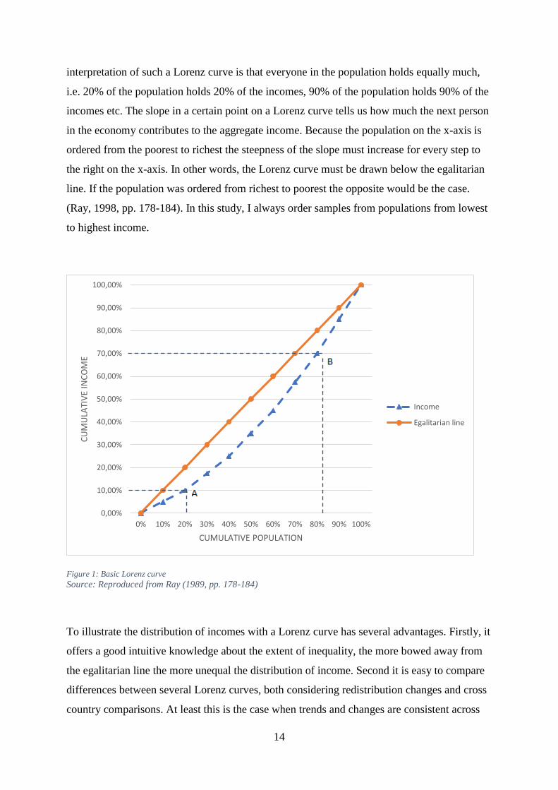
2.2.4 The Lorenz curve

The Lorenz curve is a convenient graphic illustration presenting how income is distributed

across a population, the description in the following section follow the work of Debraj Ray

(1998, pp. 178-184). Along the x-axis in Figure 1 the population is sorted in increasing order

of income. Along the y-axis the cumulative income is ordered, i.e. a scale from 0-100% where

each point represents a percentage share of the total aggregate income of the population. Now

let us have a look at point A in Figure 1, this point indicates 10% on the income-axis and 20%

on the population-axis which tells us that the 20% of the population with the lowest income

holds 10% of the aggregate incomes. Further, point B contains the information that the lower

80% in the income distribution holds 70% of the aggregate incomes. Another way to interpret

the first point (point A) is that the top 80% in the income distribution holds 90% of the

aggregate incomes and for point B that the top 20% in the income distribution holds 30% of

the aggregate incomes. The more data points the more accurate income distribution is possible

to create, still no matter how many data points that are included the far end points of the

Lorenz curve will origin at the end of the y- and x-axis. This should be interpreted as if 0% of

the population holds 0% of the aggregate incomes and that 100% of the population holds

100% of all incomes. A straight line between these two points creates the egalitarian line. The

1 Analytical weights provided in STATA were used.

14

interpretation of such a Lorenz curve is that everyone in the population holds equally much,

i.e. 20% of the population holds 20% of the incomes, 90% of the population holds 90% of the

incomes etc. The slope in a certain point on a Lorenz curve tells us how much the next person

in the economy contributes to the aggregate income. Because the population on the x-axis is

ordered from the poorest to richest the steepness of the slope must increase for every step to

the right on the x-axis. In other words, the Lorenz curve must be drawn below the egalitarian

line. If the population was ordered from richest to poorest the opposite would be the case.

(Ray, 1998, pp. 178-184). In this study, I always order samples from populations from lowest

to highest income.

Figure 1: Basic Lorenz curve

Source: Reproduced from Ray (1989, pp. 178-184)

To illustrate the distribution of incomes with a Lorenz curve has several advantages. Firstly, it

offers a good intuitive knowledge about the extent of inequality, the more bowed away from

the egalitarian line the more unequal the distribution of income. Second it is easy to compare

differences between several Lorenz curves, both considering redistribution changes and cross

country comparisons. At least this is the case when trends and changes are consistent across

0,00%

10,00%

20,00%

30,00%

40,00%

50,00%

60,00%

70,00%

80,00%

90,00%

100,00%

0% 10% 20% 30% 40% 50% 60% 70% 80% 90% 100%

CU

MU

LATI

VE

INC

OM

E

CUMULATIVE POPULATION

Income

Egalitarian line

15

the whole distribution. All points of a Lorenz curve must be below another if the first should

be considered more unequal than the first distribution. This criterion for comparison is called

the Lorenz Criterion (Ray, 1998, pp. 181). In the cases when two Lorenz curves cross each

other a general conclusion that one distribution is more unequal is not possible. Still it is

possible to draw conclusions on inequality trends for certain parts of the distribution which

fulfil the Lorenz criterion.

2.2.5 The Gini coefficient

The Gini coefficient is due to its simplicity a rather convenient measure on inequality which is

used by both researchers and policy makers. I will explain how it is calculated and hopefully

this will bring a better understanding also about the coefficient’s drawbacks. There are two

ways to explain how the Gini coefficient is calculated, one pure mathematical and a more

graphic explanation. I will only describe the graphic since it conveniently connects to the

Lorenz curve. Recall that the Lorenz graph both had the egalitarian line and the Lorenz curve

which is bowed out south east from the egalitarian line (see Figure 2). By simply calculating

the ratio of the area between the egalitarian line and the Lorenz curve (bright area in Figure

2), to the full area below the egalitarian line (dark plus bright area in Figure 2), the Gini

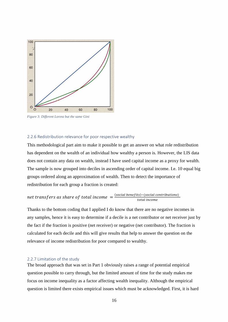
coefficient is created2 (Ray, 1998, pp.188-191). An obvious drawback with the Gini

coefficient though is that a single Gini in theory could represent infinite many different

distributions since the Gini is a product of two areas (Figure 3).

Figure 2: Graphic derivation of the Gini coefficient Source: Own illustration

2 For the empirical part of this study the Stata commando ineqdec0 was used.

16

2.2.6 Redistribution relevance for poor respective wealthy

This methodological part aim to make it possible to get an answer on what role redistribution

has dependent on the wealth of an individual how wealthy a person is. However, the LIS data

does not contain any data on wealth, instead I have used capital income as a proxy for wealth.

The sample is now grouped into deciles in ascending order of capital income. I.e. 10 equal big

groups ordered along an approximation of wealth. Then to detect the importance of

redistribution for each group a fraction is created:

𝑛𝑒𝑡 𝑡𝑟𝑎𝑛𝑠𝑓𝑒𝑟𝑠 𝑎𝑠 𝑠ℎ𝑎𝑟𝑒 𝑜𝑓 𝑡𝑜𝑡𝑎𝑙 𝑖𝑛𝑐𝑜𝑚𝑒 =(𝑠𝑜𝑐𝑖𝑎𝑙 𝑏𝑒𝑛𝑒𝑓𝑖𝑡𝑠)−(𝑠𝑜𝑐𝑖𝑎𝑙 𝑐𝑜𝑛𝑡𝑟𝑖𝑏𝑢𝑡𝑖𝑜𝑛𝑠)

𝑡𝑜𝑡𝑎𝑙 𝑖𝑛𝑐𝑜𝑚𝑒

Thanks to the bottom coding that I applied I do know that there are no negative incomes in

any samples, hence it is easy to determine if a decile is a net contributor or net receiver just by

the fact if the fraction is positive (net receiver) or negative (net contributor). The fraction is

calculated for each decile and this will give results that help to answer the question on the

relevance of income redistribution for poor compared to wealthy.

2.2.7 Limitation of the study

The broad approach that was set in Part 1 obviously raises a range of potential empirical

question possible to carry through, but the limited amount of time for the study makes me

focus on income inequality as a factor affecting wealth inequality. Although the empirical

question is limited there exists empirical issues which must be acknowledged. First, it is hard

Figure 3: Different Lorenz but the same Gini

17

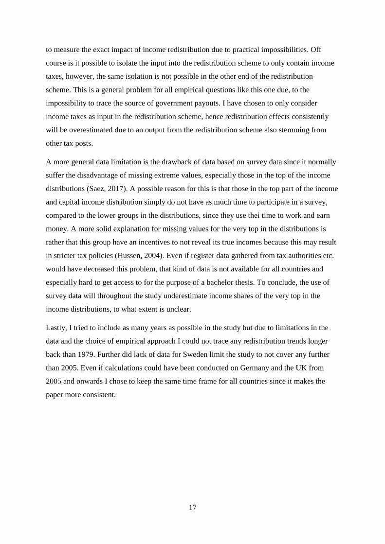
to measure the exact impact of income redistribution due to practical impossibilities. Off

course is it possible to isolate the input into the redistribution scheme to only contain income

taxes, however, the same isolation is not possible in the other end of the redistribution

scheme. This is a general problem for all empirical questions like this one due, to the

impossibility to trace the source of government payouts. I have chosen to only consider

income taxes as input in the redistribution scheme, hence redistribution effects consistently

will be overestimated due to an output from the redistribution scheme also stemming from

other tax posts.

A more general data limitation is the drawback of data based on survey data since it normally

suffer the disadvantage of missing extreme values, especially those in the top of the income

distributions (Saez, 2017). A possible reason for this is that those in the top part of the income

and capital income distribution simply do not have as much time to participate in a survey,

compared to the lower groups in the distributions, since they use thei time to work and earn

money. A more solid explanation for missing values for the very top in the distributions is

rather that this group have an incentives to not reveal its true incomes because this may result

in stricter tax policies (Hussen, 2004). Even if register data gathered from tax authorities etc.

would have decreased this problem, that kind of data is not available for all countries and

especially hard to get access to for the purpose of a bachelor thesis. To conclude, the use of

survey data will throughout the study underestimate income shares of the very top in the

income distributions, to what extent is unclear.

Lastly, I tried to include as many years as possible in the study but due to limitations in the

data and the choice of empirical approach I could not trace any redistribution trends longer

back than 1979. Further did lack of data for Sweden limit the study to not cover any further

than 2005. Even if calculations could have been conducted on Germany and the UK from

2005 and onwards I chose to keep the same time frame for all countries since it makes the

paper more consistent.

18

Part 3 Part 3 contains a careful examination of the results from the empirical application on income

redistribution trends in Germany, Sweden and the UK in 1979-2005.

3.1 Empirical results In this section, the most relevant graphs will be shown for trends and developments of the

Gini coefficient and the Lorenz curve. Consistently distribution measures will be shown, both

before and after government intervention, thereby the redistribution effect is documented.

Last, I will extract the most relevant finding concerning the question on redistribution

relevance for different groups in the wealth distribution. For the readers’ convenience, some

linguistic simplifications are used; income inequality is referred to as inequality, pre

redistribution income inequality is referred to as pre inequality, post redistribution income

inequality is referred to as post inequality. Hence pre and post redistribution only will be

referred to as pre and post. These simplifications will be used throughout the rest of the study.

Note that wealth inequality is never shortened.

3.1.1 Gini coefficients

As can be seen in Figure 4 the samples for each country do not coincide on the same years,

hence are specific comparison between years and countries unsuitable. Instead, focus will be

on trends and interesting changes in the Gini, i.e. an increase of the Gini indicates increased

income inequality and a decreasing Gini indicate decreasing income inequality. Before I

present the results, some reference points will be given, this will make the interpretations of

Gini changes easier. Among the OECD countries do the post Ginis vary a lot, e.g. Denmark

had the lowest post Gini at 0,25 in 2012 while the US had a post Gini at 0,40 for the same

year. Only Turkey, Mexico and Chile had a higher post Gini than the US. An average post

Gini for the whole OECD in 2012 was at 0,32. Hopefully these reference points are helpful in

understanding the following part.

The most dramatic increase happened in the UK between 1979 and 1986 when the pre Gini

rose from 0,42 up to 0,51. Except of a clear increase by 0,03 points 1991-1994 the pre Gini

has been at a stable level and even decreased slightly 1994-2004. In line with the UK has

Sweden also faced a steady increase in their pre Gini with 0,09 points up until 1995. Similar

to the UK did Germany also experience a distinct increase of the pre Gini during the first half

of the 80’s. Further, a slight increase is observed in 1989-2000, a period covering the German

reunification and hence inclusion of East Germany in the data. From 2000 is the increase once

19

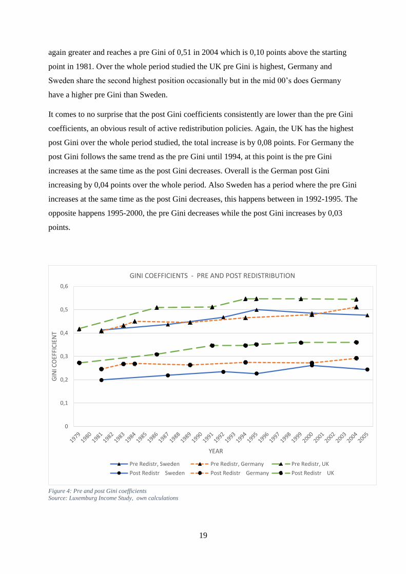
again greater and reaches a pre Gini of 0,51 in 2004 which is 0,10 points above the starting

point in 1981. Over the whole period studied the UK pre Gini is highest, Germany and

Sweden share the second highest position occasionally but in the mid 00’s does Germany

have a higher pre Gini than Sweden.

It comes to no surprise that the post Gini coefficients consistently are lower than the pre Gini

coefficients, an obvious result of active redistribution policies. Again, the UK has the highest

post Gini over the whole period studied, the total increase is by 0,08 points. For Germany the

post Gini follows the same trend as the pre Gini until 1994, at this point is the pre Gini

increases at the same time as the post Gini decreases. Overall is the German post Gini

increasing by 0,04 points over the whole period. Also Sweden has a period where the pre Gini

increases at the same time as the post Gini decreases, this happens between in 1992-1995. The

opposite happens 1995-2000, the pre Gini decreases while the post Gini increases by 0,03

points.

0

0,1

0,2

0,3

0,4

0,5

0,6

GIN

I CO

EFFI

CIE

NT

YEAR

GINI COEFFICIENTS - PRE AND POST REDISTRIBUTION

Pre Redistr, Sweden Pre Redistr, Germany Pre Redistr, UK

Post Redistr Sweden Post Redistr Germany Post Redistr UK

Figure 4: Pre and post Gini coefficients

Source: Luxemburg Income Study, own calculations

20

To summarize; The Swedish pre Gini increased by 0,07 points, the post Gini increased by

0,04 points. The German pre Gini increased by 0,10 points, the post Gini increased by 0,05

points. In the UK did the pre Gini increase by 0,12 points, the post Gini increased by 0,09

points. Finally did the UK experience the highest pre and post Gini for all periods while

Sweden had the lowest post Gini for all periods, since the 90’s was the German post Gini

closer to the Swedish than the post Gini for the UK. Exact numbers of the pre and post Gini

coefficients for each country and years is presented in Appendix 1.

3.1.2 Lorenz curves

In this section I present two types of Lorenz curves for each country and year, one for pre-

redistribution data and one for post redistribution data. In addition to the graphs, tables are

presented containing information of changes in income share of the total income for three

groups in the income distribution, the bottom 20%, the bottom 50% and the bottom 70%.

These will be stand-alone tables that are not commented in the text but function as an

underpinning to the Lorenz curves. More detailed tables on pre and post inequality for each

country during all years studied, are presented in Appendix2.

Sweden

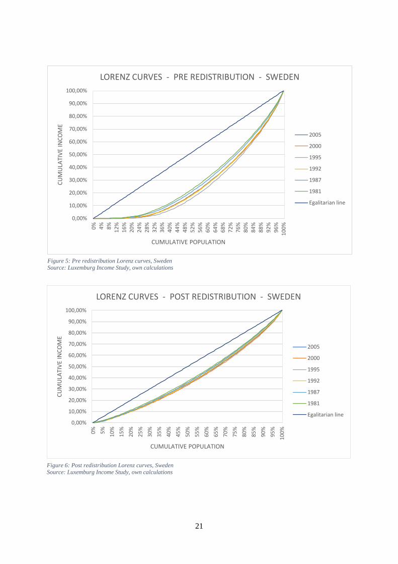
The pre curves for Sweden show that the income inequality overall has increased in the period

1981-2005 although fluctuations are observed. The greatest increase in pre inequality

happened in 1981-1995 where the income share of the bottom half of the income distribution

dropped by 6,88% points, the greatest share of the decrease were in 1992-1995. In 1995-2000

are pre inequality decreasing to the level of 1992, it stays at this level also in 2005.

Similar to the results on the Gini coefficients the trend for the Lorenz curves is that the post

inequality follows the trend of the pre inequality. Nevertheless, the post inequality decreases

in 1992-1995 at the same time as the pre inequality increases. In the next period studied

(1995-2000) the post inequality increases though. Finally, the ending five years between 2000

and 2005 show a slight decrease in post inequality. Dependent on the year studied there are 2-

7% of the population who gain zero income on their own (the trend indicates more zero

income earners over time), all receive positive income after income redistribution.

21

0,00%

10,00%

20,00%

30,00%

40,00%

50,00%

60,00%

70,00%

80,00%

90,00%

100,00%

0%

5%

10

%

15

%

20

%

25

%

30

%

35

%

40

%

45

%

50

%

55

%

60

%

65

%

70

%

75

%

80

%

85

%

90

%

95

%

10

0%

CU

MU

LATI

VE

INC

OM

E

CUMULATIVE POPULATION

LORENZ CURVES - POST REDISTRIBUTION - SWEDEN

2005

2000

1995

1992

1987

1981

Egalitarian line

0,00%

10,00%

20,00%

30,00%

40,00%

50,00%

60,00%

70,00%

80,00%

90,00%

100,00%0

%

4%

8%

12

%

16

%

20

%

24

%

28

%

32

%

36

%

40

%

44

%

48

%

52

%

56

%

60

%

64

%

68

%

72

%

76

%

80

%

84

%

88

%

92

%

96

%

10

0%

CU

MU

LATI

VE

INC

OM

E

CUMULATIVE POPULATION

LORENZ CURVES - PRE REDISTRIBUTION - SWEDEN

2005

2000

1995

1992

1987

1981

Egalitarian line

Figure 5: Pre redistribution Lorenz curves, Sweden Source: Luxemburg Income Study, own calculations

Figure 6: Post redistribution Lorenz curves, Sweden Source: Luxemburg Income Study, own calculations

22

United Kingdom

The pre inequality has increased quite a lot in the UK over the period studied. The greatest

increases occurred 1979-1986 and 1991-1994 when the bottom half of the income distribution

lost 7,30 respective 2,77% points of the total income share. From 1994 to 2004 the pre

inequality is generally stable, the bottom half of the income distribution gain a slight income

share. The increased inequality over time which is observed before government redistribution,

re-appears after redistribution if not to the same extent. The increased post inequality is

mainly driven during the years of 1979-1991. At last is the inequality relatively stable

between 1991 and 2004, still there are some variations for certain groups in the income

distribution. In several sample years more than 10% of the population do not gain any income

before redistribution, this is clearly higher than for both Germany and Sweden, nevertheless

almost all gain positive income after government redistribution.

SWEDEN PRE-REDISTRIBUTION SHARE OF

TOTAL INCOME (%)

POST-REDISTRIBUTION

SHARE OF TOTAL INCOME (%)

CHANGE FROM PRE TO POST

REDISTR. (%-POINTS)

POP. SHARE 20% 50% 70% 20% 50% 70% 20% 50% 70%

1981 1,33 20,92 44,42 11,22 36,67 57,82 +9,89 +15,75 +13,4

2005 0,35 16,97 40,00 10,15 34,21 55,07 +9,80 +17,24 +15,07

CHANGE (%-

POINTS)

-0,98 -3,95 -4,42 -1,07 -2,46 -2,75

Figure 7: Overview table of redistribution trends, Sweden Source: Luxemburg Income Study, own calculations

23

Figure 9: Post redistribution Lorenz curves, the UK Source: Luxemburg Income Study, own calculations

0,00%

10,00%

20,00%

30,00%

40,00%

50,00%

60,00%

70,00%

80,00%

90,00%

100,00%

0%

5%

10

%

15

%

20

%

25

%

30

%

35

%

40

%

45

%

50

%

55

%

60

%

65

%

70

%

75

%

80

%

85

%

90

%

95

%

10

0%

CU

MU

LATI

VE

INC

OM

E

CUMULATIVE POPULATION

LORENZ CURVE - POST REDISTRIBUTION - UNITED KINGDOM

2004

1999

1995

1994

1991

1986

1979

Egalitarian line

0,00%

10,00%

20,00%

30,00%

40,00%

50,00%

60,00%

70,00%

80,00%

90,00%

100,00%0

%

5%

10

%

15

%

20

%

25

%

30

%

35

%

40

%

45

%

50

%

55

%

60

%

65

%

70

%

75

%

80

%

85

%

90

%

95

%

10

0%

CU

MU

LATI

VE

INC

OM

E

CUMULATIVE POPULATION

LORENZ CURVES - PRE REDISTRIBUTION - UNITED KINGDOM

2004

1999

1995

1994

1991

1986

1979

Egalitarian line

Figure 8: Pre redistribution Lorenz curves, the UK Source: Luxemburg Income Study, own calculations

24

Germany

In the period studied the pre inequality in general is clearly increasing, one exception is a

decreases in pre inequality 1984-1989. Otherwise are three major increases in pre inequality

observed; 1981-1983, 1989-1994 and 2000-2004. Worth to notice are the shifts in the lower

part of the income distribution; in 1981 17% of the population gain no income before

redistribution, a number which lies at approximately 5% all other years included in the study.

Irrespective of year observed all individuals gain positive income after redistribution.

In the post graph are smaller shifts observed in the Lorenz curves. Still there is a small

increase in inequality between 1981 and 1983, thereafter is the inequality relatively stable

until 2000, except of a clear increase in income share for the bottom half of the income

distribution in 1994-2000. Finally, post inequality increased slightly 2000-2004.

UK. PRE-REDISTRIBUTION SHARE

OF TOTAL INCOME (%)

POST-REDISTRIBUTION

SHARE OF TOTAL INCOME (%)

CHANGE FROM PRE TO

POST REDISTR. (%-POINTS)

POP. SHARE 20% 50% 70% 20% 50% 70% 20% 50% 70%

1979 0,82 21,18 43,64 8,89 31,62 52,51 +8,07 +10,44 +8,87

2004 0,05 12,14 34,21 7,48 27,50 47,12 +7,43 +15,36 +12,91

CHANGE (%-

POINTS)

-0,77 -9,04 -9,43 -1,41 -4,12 -5,39

Figure 10: Overview table on redistribution trends, the UK Source: Luxemburg Income Study, own calculations

25

Figure 11: Pre redistribution Lorenz curves, Germany Source: Luxemburg Income Study, own calculations

Figure 12: Post redistributioin Lorenz curces, Germany Source: Luxemburg Income Study, own calculations

0,00%

10,00%

20,00%

30,00%

40,00%

50,00%

60,00%

70,00%

80,00%

90,00%

100,00%

0%

4%

8%

12

%

16

%

20

%

24

%

28

%

32

%

36

%

40

%

44

%

48

%

52

%

56

%

60

%

64

%

68

%

72

%

76

%

80

%

84

%

88

%

92

%

96

%

10

0%

CU

MU

LATI

VE

INC

OM

E

CUMULATIVE POPULATION

LORENZ CURVES - PRE REDISTRIBUTION - GERMANY

2004

2000

1994

1989

1984

1983

1981

Egalitarian line

0,00%

10,00%

20,00%

30,00%

40,00%

50,00%

60,00%

70,00%

80,00%

90,00%

100,00%

0%

5%

10

%

15

%

20

%

25

%

30

%

35

%

40

%

45

%

50

%

55

%

60

%

65

%

70

%

75

%

80

%

85

%

90

%

95

%

10

0%

CU

MU

LATI

VE

INC

OM

E

CUMULATIVE POPULATION

LORENZ CURVES - POST REDISTRIBUTION - GERMANY

2004

2000

1994

1989

1984

1983

1981

Egalitarian line

26

To summarize this section it is clear that all countries execute comprehensive income

redistribution where almost no individuals have zero incomes after redistribution. Sweden has

throughout the period studied had the lowest share of people with no income and the UK does

generally have more people with no income (Germany has one extreme year with high share

of people with no income, otherwise the income concentration is lower). At last is it clear that

the Swedish and the German governments have kept post inequality relatively stable towards

the background that both countries (especially Germany) have experienced distinct increases

in pre inequality. The UK has over the period studied redistributed the least and Sweden the

most, a result which per se do not say anything of which country that has the most equal

income distribution. However, in the case of this study it happens to be that the country which

redistributes the most, Sweden, also has the lowest income inequalities and the UK has the

greatest income inequality.

3.1.3 Relevance of redistribution for wealthy respective poor

The underlying assumption for this section is that capital income is a proper proxy for wealth,

capital income then has been ordered along the x-axis in ascending order, i.e. wealthier to the

right and poor to the left in the graphs presented. Note that there are no negative incomes

present in the data underlying the graphs, this guarantees that all positive values represent net

receivers and all negative values represent net contributors. With that in mind a negative

sloped curve would imply that wealthier contribute (to the redistribution scheme) with a

greater share of their total income than is the case for poor. However, the results from this

study points in another direction which will be explained below, similar as was done for the

Lorenz curves, each country will be examined separately.

GERMANY PRE-REDISTR. SHARE OF TOTAL

INCOME (%)

POST-REDISTR. SHARE OF

TOTAL INCOME (%)

CHANGE FROM PRE TO

POST REDISTR. (%-POINTS)

POP. SHARE 20% 50% 70% 20% 50% 70% 20% 50% 70%

1981 0,61 22,27 44,98 10,30 33,71 54,34 +9,69 +11,24 +9,36

2004 0,24 14,81 36,72 8,96 31,74 51,95 +8,72 +16,93 +15,23

CHANGE (%-

POINTS)

-0,37 -7,46 -8,26 -1,34 -1,97 -2,39

Figure 13: Overview table on redistribution trends, Germany Source: Luxemburg Income Study, own calculations

27

Sweden

Clearly, the Swedish graph (Figure 14) does not correspond to a steady negative slope which

would indicate wealthier (high capital income) to contribute relatively more than poor (low

capital income). The first surprising result is that almost all deciles during all years (except of

3 deciles 1987) have positive values, i.e. are net receivers. I will discuss the credibility of

these results more in the discussion section under Part 4. More expected is that the poorest in

almost all years gain relatively more of redistribution compared to the wealthier groups.

Another interesting result is the u-shape present for most years, which implies that the gains

from redistribution increases with wealth. This relationship is true for most years between the

5th and 9th decile, but for the 10th decile the gain from redistribution as share of total income

decreases a lot. To conclude, there are three important results to emphasize; The poor gain the

most of redistribution in relative measures (redistribution gain as share of total income), the

middle deciles gain relatively less than the wealthier deciles, and the very top decile receive

relatively less than the 9th decile.

Figure 14: Redistribution relevance along the capital income distribution, Sweden Source: Luxemburg Income Study, own calculations

-0,1

-0,05

0

0,05

0,1

0,15

0,2

0,25

0,3

0 1 2 3 4 5 6 7 8 9 10

NET

TR

AN

SFER

S A

S SH

AR

E O

F TO

TAL

INC

OM

E

DECILES

REDISTRIBUTION GAINS AS SHARE OF TOTAL INCOME, PICTURED ACROSS THE CAPITAL INCOME DISTRIBUTION - SWEDEN

2005

2000

1995

1992

1987

1981

28

Germany

In the case of Germany there is only one decile one year that is a net contributor (Figure 15),

otherwise all deciles are net receivers similar as it was for Sweden. The poorest group in all

years receives relatively more than all wealthier groups, except of this clear difference any

obvious patterns are difficult to find. The U-shape that we saw in the graph for Sweden is not

as clear for Germany in all years, instead there is a peak in the 6th and 7th decile for Germany.

Interestingly the top decile is never taking on the lowest value for any year in Germany, i.e.

that the relative importance of redistribution gains always has been higher for the richest

group compared to other groups in the wealth distribution.

Figure 15: Redistribution relevance along the capital income distribution, Germany

Source: Luxemburg Income Study, own calculations

United Kingdom

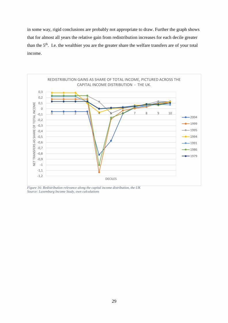
The graph for the UK (Figure 16) differ considerably from the other countries in two aspects.

First it has way more deciles that are net contributors, e.g. the poorest 60% of the population

are net contributors in 2004 according to these results. Secondly three years (1986, 1999,

2004) are characterized by extremely low values for the 4th decile, even below minus 1 for

1986 and 1999. This implies that the 4th decile in 1986 and 1999 contribute more than they

have as total income. This result is extreme and brings worries that the results might be biased

-0,05

0

0,05

0,1

0,15

0,2

0,25

0,3

0 1 2 3 4 5 6 7 8 9 10

NET

TR

AN

SFER

S A

S SH

AR

E O

F TO

TAL

INC

OM

E

DECILES

REDISTRIBUTION GAINS AS SHARE OF TOTAL INCOME, PICTURED ACROSS THE CAPITAL INCOME DISTRIBUTION - GERMANY

2004

2000

1994

1989

1984

1983

29

in some way, rigid conclusions are probably not appropriate to draw. Further the graph shows

that for almost all years the relative gain from redistribution increases for each decile greater

than the 5th. I.e. the wealthier you are the greater share the welfare transfers are of your total

income.

Figure 16: Redistribution relevance along the capital income distribution, the UK Source: Luxemburg Income Study, own calculations

-1,2

-1,1

-1

-0,9

-0,8

-0,7

-0,6

-0,5

-0,4

-0,3

-0,2

-0,1

0

0,1

0,2

0,3

0 1 2 3 4 5 6 7 8 9 10

NET

TR

AN

SFER

S A

S SH

AR

E O

F TO

TAL

INC

OM

E

DECILES

REDISTRIBUTION GAINS AS SHARE OF TOTAL INCOME, PICTURED ACROSS THE CAPITAL INCOME DISTRIBUTION - THE UK.

2004

1999

1995

1994

1991

1986

1979

30

Part 4

4.1 Discussion The results from both the Gini coefficients and the Lorenz curves are unambiguous, both pre

and post inequality have increased in the UK, Sweden and Germany from the 80’s until the

mid 00’s. The UK experienced the greatest increase in pre inequality while Sweden had the

smallest increase. Also, the post inequality increased the most in the UK while Sweden and

Germany had about the same increase. Further do my results on absolute inequality numbers

confirm the perception, formulated by Piketty and Zucman (2014), of the UK as a country

characterized by high post inequalities and Sweden as a country with less post inequality.

Throughout the whole period subject to the study Sweden and Germany redistributed about as

much if one look at the change in pre and post inequality for the 20th, 50th and 70th percentile,

still Sweden has the least unequal post income distribution of the three countries in all years

included in the study.

The varying results on post inequalities in the three countries give support to the argument by

Saez (2017) that governments indeed can affect the post inequality levels. Still there is a

dominant trend apparent in all three countries; post inequality follow the trend of pre

inequality almost without exceptions, something that has been observed in several other

studies as well (Förster and delle Politiche Sociali, 2011; “Poverty and Shared Prosperity

2016,” n.d.). The dominance of pre inequality trends being reflected in post inequality raises

several questions on the role of the governments in the three countries; are they not capable or

maybe not even interested in keeping the post inequality stable? Possible explanations may be

that governments have a great concern for negative economic effects, described by Bastani

and Lundberg (2016) and Saez (2017), as a result of more progressive redistribution policies,

and less concerns for negative effects which Finnie et al. (2006) argue can arise from great

income and wealth inequalities. Certainly, varying perceptions on fairness could be another

possible explanation for the acceptance Sweden, the UK and Germany show towards

increased post inequality. It is needless to say that it is out of scope of this study to bring

clarity in the importance of each factor, but the range of potential factors affecting post

inequality is quite telling considering the wide range of empirical questions that are

interesting to study further.

However, what is rather sure is that the role and persistence of status quo, which Zoutman et

al. (2016) discusses, indeed makes it harder to incorporate a desire to keep post inequalities

stable simultaneous to increasing pre inequalities. In order to succeed with such a desire, the

31

legislators would be required to implement a more progressive income redistribution each

time the pre inequality increases. Obviously, this will disadvantage high income earner which

constitutes an important voting group to legislators. Consequently, policy changes considering

redistribution are hard to implement and status quo function as an inertia in the political

system (Zoutman et al., 2016).

Now imagine a scenario where a government has the ambition and is able to keep post

inequalities at a stable level while the pre inequality continued increasing, could that be a

sustainable development considering the risk of societal tension? Again, the answer is likely

to be found in peoples’ perception of fairness. If the group who gain an increased income

share, of the total income, perceive themselves worthy the gain then problem will occur when

a strong redistribution scheme redistributes the gains. Societal tension should therefore be

probable to appear from “above” if these income groups believe the development to be a

result of their own efforts rather than a result of structural changes on the labor market or

inheritance inequality which leads to increased income shares for some groups.

Something worth coming back to is that income redistribution is not the sole driving factor to

wealth inequality and opportunities for individual monetary prosperity. For instance, policy

changes related to welfare systems in respective country could possibly make the welfare

carrying a larger redistributive capacity. A post redistribution inequality trend should

therefore not be treated as a complete indicator on whether wealth inequality has increased or

not, an idea also shared by the current Swedish Minister of Finance Magdalena Andersson

(Hellquist, 2017).

The empirical part of the study was twofold; the first part considered trends in redistribution

which have been discussed above, the second part asked the question how relevant the

redistribution effect is for wealthy respective poor. This second part of the empirical part

brought two quite surprising results. First, that almost all deciles in all years for all three

countries were net receivers, i.e. they received more monetary social benefits than they

contributed with to the redistribution scheme. An obvious question then is how a country

could be run where all are net receivers of monetary transfers and nobody are net contributors.

Part of the answer could possibly be that the state receives monetary means through a variety

of channels except income taxes, i.e. consumption taxes and revenues from public enterprises

etc. Still these results are very surprising and potentially not accurate, conclusion should

therefore be conducted with caution. The second surprising indication from my results was

that the wealthier groups, i.e. people with higher capital income, in general received more

32

social benefits (as a share of their total income) compared to the groups in the middle of the

wealth distribution. A possible explanation for this could be the existence of inheritance

delay, i.e. that some parents die young and consequently children at the same age will inherit

at different points in time. Individuals inheriting at an early age obviously are more likely to

earn capital income since they have capital to administer, hence they are categorized as

wealthy in this study. Now add that those groups with parents dying at young age to a greater

extent are low income earners and hence are more probable to receive more benefits from the

government. These factors in combination possibly could explain that the wealthiest also gain

relatively more from redistribution than the deciles in the middle of the wealth distribution.

Moreover, the grouping from poor to wealthy is possibly close to an ordering of people from

young to old since elderly naturally have had more time to accumulate wealth, which

potentially could generate capital income, compared to young people. By perceiving the

wealth distribution (estimated with capital income as a proxy for wealth) like an age

distribution the shape of the graphs can be better understood; The young are to a greater

extent studying instead of working compared to the elderly, i.e. they receive study grants from

the state but contribute little through income taxation. Further, the middle-aged groups work

relatively much and cost little to the society, and the elderly in the samples used (age 18-65)

are probably starting to cost society due to early pensions, health care costs etc. This

demographic aspect could also serve as a potential explanation to the U-shape tendency that

could be seen in all graphs on the relative gain from redistribution (Figure 14-16). To be able

to isolate for the mentioned factors a narrower age group to study could have been an

rewarding complement. The relative gain of redistribution across a wealth distribution with

similar background variables would then had been possible to observe.

The pre and post redistribution data for each country also brought clarity in how great share of

the population that had zero income before government intervention. This number roughly

should correspond to the unemployment rate for the country for a specific period, also the

share of students and other non-paid workers as housewives etc. should be reflected in the

same number. The results of my study in general are not dubious, however, the data for

Germany 1981 indicates that 17% of the population were without income. That the

unemployed, students and other non-paid workers constitutes 17% of the population is

surprising and rise doubts due to the sharp decrease of the zero income group the following

period studied (below 10% in 1983). All other years for the three countries show more

33

realistic numbers of zero income earners and the results should therefore be acknowledged as

reliable.

4.2 Concluding remarks With this study, I try to answer the research question how government policies can counteract

increasing wealth and income inequality. This research question is relevant towards the

background of studies suggesting wealth and income inequalities to increase in western

industrialized countries (Förster and delle Politiche Sociali, 2011; Piketty and Saez, 2014;

“Poverty and Shared Prosperity 2016,” n.d.; Saez and Zucman, 2016), and that such

developments are in the interest of both policy makers as well as for the public. The broad

interest in the matter is rooted in both strong perceptions of fairness (Saez, 2017) but also in a

fear that large monetary inequalities are harmful to society (Finnie et al., 2006). To answer the

research question a theoretical and an empirical approach was useful to apply. In the

theoretical part I describe the close interconnectedness between income inequality, wealth

inequality and how inheritance is problematic from a fairness perspective. Due to the great

importance of income inequality as a driving factor to wealth inequality I narrow the focus for

the empirical part to only consider the policy enforcement of income redistribution. An

application is conducted to Sweden, Germany and the UK in 1979-2005. This approach also

brought about some limitation of for the study, most important is the complexity to isolate

income redistribution from other redistribution channels controlled by a state. Therefore, the

income redistribution results consistently are overestimated. Although limitations are present,

I still find clear results from the empirical application; both pre redistribution income

inequality and post redistribution income inequality have increased in all three countries from

the beginning of the 80’s to the mid 00’s, although the magnitude vary between the countries.

The UK redistributes the least income and Sweden the most, in addition the income inequality

is the highest in the UK and the lowest in Sweden. Last, even if domestic policies generates

varying post income inequalities, no country has kept their post redistribution income

inequality at a stable level; a trend of increasing pre redistribution income inequality have,

almost without exceptions, been reflected in increasing post redistribution income inequality.

This is a worrying result for those advocating more progressive income redistribution as a

policy tool to counteract increasing income inequalities and wealth inequalities.

34

Reference list

Journal papers Armour, P., Burkhauser, R.V., Larrimore, J., 2014. Levels and Trends in US Income and its

Distribution: A Crosswalk from Market Income towards a Comprehensive Haig-

Simons Income Approach. South. Econ. J. 81, 271–293.

Atkinson, A.B., Piketty, T., Saez, E., 2011. Top incomes in the long run of history. J. Econ.

Lit. 49, 3–71.

Auerbach, A.J., 1989. Capital gains taxation and tax reform. Natl. Tax J. 42, 391–401.

Bastani, S., Lundberg, J., 2016. Political preferences for redistribution in Sweden.

Björklund, A., Jäntti, M., 2009. Intergenerational income mobility and the role of family

background. Oxf. Handb. Econ. Inequal. Oxf. Univ. Press Oxf. 491–521.

Björklund, A., Roine, J., Waldenström, D., 2012. Intergenerational top income mobility in

Sweden: Capitalist dynasties in the land of equal opportunity? J. Public Econ. 96,

474–484.

Black, S.E., Devereux, P.J., 2010. Recent developments in intergenerational mobility.

National Bureau of Economic Research.

Bowles, S., Gintis, H., 2002. The inheritance of inequality. J. Econ. Perspect. 16, 3–30.

Elinder, M., Erixson, O., Waldenström, D., 2016. Inheritance and wealth inequality: Evidence

from population registers.

Fajnzylber, P., Lederman, D., Loayza, N., 2002. What causes violent crime? Eur. Econ. Rev.

46, 1323–1357.

Finnie, R., Irvine, I., others, 2006. Mobility and gender at the top tail of the earnings

distribution. Econ. Soc. Rev. 37, 149.

Förster, M., delle Politiche Sociali, O.-D., 2011. Divided We Stand: Why inequality keeps

rising–. OECD.

Lundberg, J., Waldenström, D., 2016. DP11246 Wealth inequality in Sweden: What can we

learn from capitalized income tax data?

Meltzer, A.H., Richard, S.F., 1981. A rational theory of the size of government. J. Polit. Econ.

89, 914–927.

Ohlsson, H., Nordblom, K., 2002. Bequests, gifts, and education swedish evidence on parents

transfer behavior. Rapp. Nr Work. Pap. Econ.

Persson, T., Tabellini, G.E., 2002. Political economics: explaining economic policy. MIT

press.

Piguillem, F., Riboni, A., 2012. Dynamic bargaining over redistribution in legislatures.

35

Piketty, T., Saez, E., 2014. Inequality in the long run. Science 344, 838–843.

Piketty, T., Saez, E., 2012. A theory of optimal capital taxation. National Bureau of Economic

Research.

Piketty, T., Zucman, G., 2014. Wealth and inheritance in the long run.

Roberts, K.W., 1977. Voting over income tax schedules. J. Public Econ. 8, 329–340.

Roemer, J.E., 1993. A pragmatic theory of responsibility for the egalitarian planner. Philos.

Public Aff. 146–166.

Roine, J., Waldenström, D., 2012. On the role of capital gains in Swedish income inequality.

Rev. Income Wealth 58, 569–587.

Romer, T., 1975. Individual welfare, majority voting, and the properties of a linear income

tax. J. Public Econ. 4, 163–185.

Saez, E., 2017. Income and Wealth Inequality: Evidence and Policy Implications. Contemp.

Econ. Policy 35, 7–25.

Saez, E., Zucman, G., 2016. Wealth inequality in the United States since 1913: Evidence from

capitalized income tax data. Q. J. Econ. 131, 519–578.

Zoutman, F.T., Jacobs, B., Jongen, E.L., 2016. Redistributive politics and the tyranny of the

middle class.

Books Diamond, J., 2005. Collapse: How societies choose to fail or succeed. Penguin.

Hussen, A.M., 2004. Principles of environmental economics. Psychology Press.

Ray, D., 1998. Development economics. Princeton University Press.

Websites LIS Cross-National Data Center in Luxembourg, n.d.

Hellquist, A., 2017. Magdalena Andersson: ”Vi ska öka skatterna för de med högst

inkomster” [WWW Document]. ETC. URL http://www.etc.se/inrikes/magdalena-

andersson-vi-ska-oka-skatterna-de-med-hogst-inkomster (accessed 5.25.17).

Poverty and Shared Prosperity 2016 [WWW Document], n.d. . World Bank. URL

http://www.worldbank.org/publication/poverty-and-shared-prosperity/en (accessed

4.10.17).

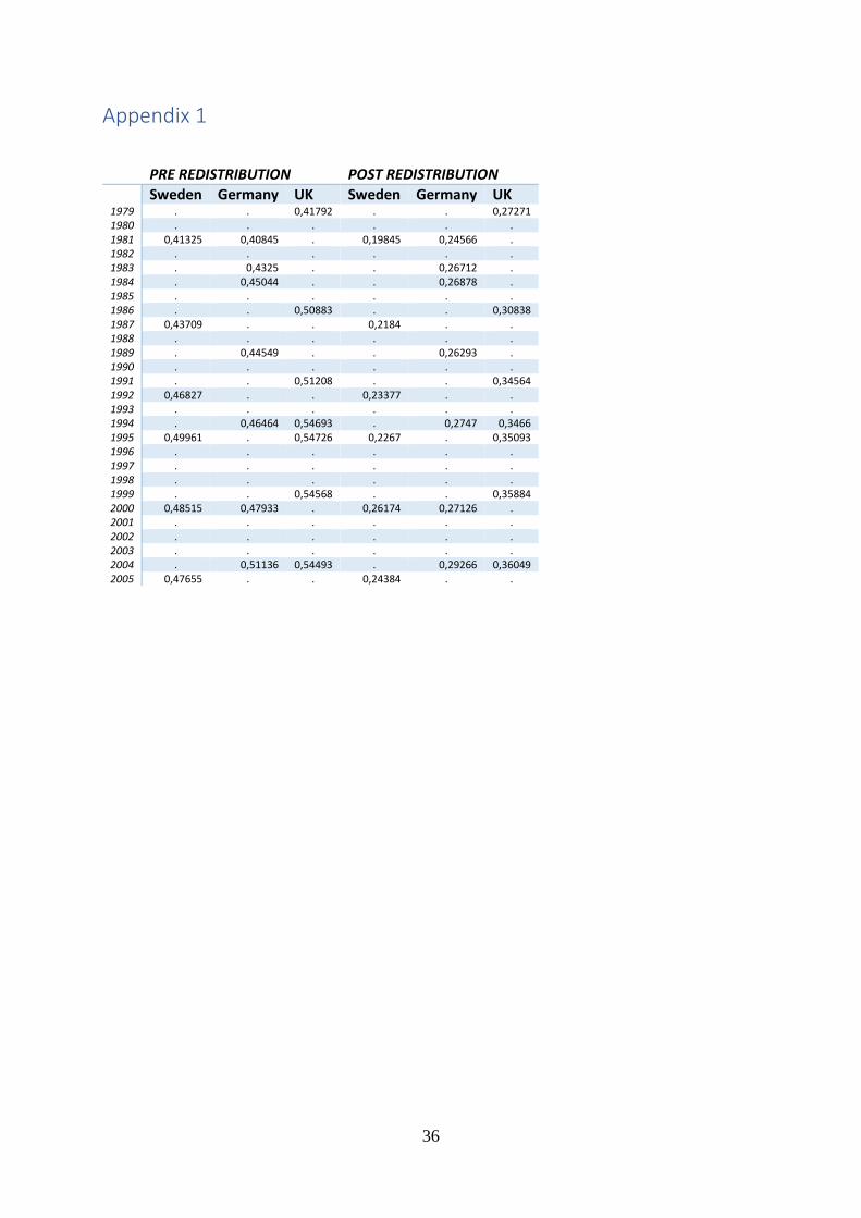
36

Appendix 1

PRE REDISTRIBUTION POST REDISTRIBUTION Sweden Germany UK Sweden Germany UK

1979 . . 0,41792 . . 0,27271 1980 . . . . . . 1981 0,41325 0,40845 . 0,19845 0,24566 . 1982 . . . . . . 1983 . 0,4325 . . 0,26712 . 1984 . 0,45044 . . 0,26878 . 1985 . . . . . . 1986 . . 0,50883 . . 0,30838 1987 0,43709 . . 0,2184 . . 1988 . . . . . . 1989 . 0,44549 . . 0,26293 . 1990 . . . . . . 1991 . . 0,51208 . . 0,34564 1992 0,46827 . . 0,23377 . . 1993 . . . . . . 1994 . 0,46464 0,54693 . 0,2747 0,3466 1995 0,49961 . 0,54726 0,2267 . 0,35093 1996 . . . . . . 1997 . . . . . . 1998 . . . . . . 1999 . . 0,54568 . . 0,35884 2000 0,48515 0,47933 . 0,26174 0,27126 . 2001 . . . . . . 2002 . . . . . . 2003 . . . . . . 2004 . 0,51136 0,54493 . 0,29266 0,36049 2005 0,47655 . . 0,24384 . .

37

Appendix 2

Table of Lorenz curves for Sweden

Pre redistribution Cumulative

population 2005 2000 1995 1992 1987 1981

0% 0.00% 0.00% 0.00% 0.00% 0.00% 0.00% 1% 0.00% 0.00% 0.00% 0.00% 0.00% 0.00% 2% 0.00% 0.00% 0.00% 0.00% 0.00% 0.00% 3% 0.00% 0.00% 0.00% 0.00% 0.00% 0.00% 4% 0.00% 0.00% 0.00% 0.00% 0.00% 0.00% 5% 0.00% 0.00% 0.00% 0.00% 0.01% 0.00% 6% 0.00% 0.00% 0.00% 0.01% 0.02% 0.01% 7% 0.00% 0.00% 0.00% 0.02% 0.04% 0.02% 8% 0.00% 0.00% 0.00% 0.03% 0.07% 0.04% 9% 0.00% 0.00% 0.01% 0.04% 0.10% 0.08% 10% 0.00% 0.01% 0.01% 0.07% 0.15% 0.12% 11% 0.01% 0.01% 0.02% 0.10% 0.19% 0.18% 12% 0.01% 0.02% 0.03% 0.14% 0.25% 0.24% 13% 0.02% 0.03% 0.05% 0.18% 0.32% 0.32% 14% 0.04% 0.05% 0.07% 0.23% 0.39% 0.42% 15% 0.06% 0.07% 0.10% 0.29% 0.48% 0.53% 16% 0.09% 0.10% 0.13% 0.36% 0.58% 0.65% 17% 0.13% 0.13% 0.17% 0.43% 0.68% 0.79% 18% 0.19% 0.18% 0.22% 0.52% 0.81% 0.95% 19% 0.26% 0.25% 0.28% 0.62% 0.95% 1.13% 20% 0.35% 0.33% 0.34% 0.73% 1.10% 1.33% 21% 0.47% 0.43% 0.42% 0.86% 1.28% 1.55% 22% 0.60% 0.56% 0.51% 1.01% 1.48% 1.81% 23% 0.77% 0.71% 0.61% 1.17% 1.72% 2.09% 24% 0.96% 0.89% 0.73% 1.35% 1.97% 2.41% 25% 1.19% 1.10% 0.86% 1.55% 2.27% 2.76% 26% 1.44% 1.35% 1.01% 1.77% 2.59% 3.16% 27% 1.74% 1.64% 1.19% 2.02% 2.95% 3.58% 28% 2.06% 1.95% 1.38% 2.30% 3.35% 4.04% 29% 2.43% 2.30% 1.61% 2.62% 3.78% 4.55% 30% 2.83% 2.69% 1.86% 2.97% 4.24% 5.10% 31% 3.27% 3.12% 2.13% 3.36% 4.73% 5.67% 32% 3.75% 3.59% 2.45% 3.78% 5.26% 6.26% 33% 4.26% 4.10% 2.79% 4.23% 5.81% 6.89% 34% 4.80% 4.63% 3.18% 4.72% 6.39% 7.53% 35% 5.37% 5.20% 3.61% 5.25% 7.00% 8.19% 36% 5.97% 5.80% 4.07% 5.80% 7.64% 8.88% 37% 6.60% 6.42% 4.57% 6.38% 8.31% 9.59% 38% 7.25% 7.07% 5.11% 6.99% 9.00% 10.33% 39% 7.93% 7.75% 5.68% 7.62% 9.71% 11.10% 40% 8.63% 8.45% 6.29% 8.28% 10.46% 11.89% 41% 9.36% 9.17% 6.93% 8.96% 11.22% 12.70% 42% 10.12% 9.92% 7.61% 9.68% 12.01% 13.53% 43% 10.89% 10.70% 8.32% 10.42% 12.82% 14.39% 44% 11.69% 11.50% 9.05% 11.19% 13.66% 15.26% 45% 12.52% 12.32% 9.81% 12.00% 14.52% 16.15% 46% 13.36% 13.16% 10.61% 12.82% 15.40% 17.07% 47% 14.23% 14.03% 11.42% 13.67% 16.31% 18.00% 48% 15.13% 14.91% 12.27% 14.55% 17.24% 18.95% 49% 16.04% 15.82% 13.14% 15.46% 18.19% 19.92% 50% 16.97% 16.75% 14.04% 16.39% 19.17% 20.92% 51% 17.93% 17.70% 14.97% 17.35% 20.17% 21.92% 52% 18.90% 18.67% 15.92% 18.34% 21.18% 22.95% 53% 19.90% 19.66% 16.91% 19.35% 22.22% 23.99% 54% 20.91% 20.69% 17.91% 20.39% 23.27% 25.05% 55% 21.95% 21.73% 18.94% 21.44% 24.34% 26.13% 56% 23.01% 22.79% 20.00% 22.52% 25.44% 27.22% 57% 24.09% 23.86% 21.09% 23.61% 26.55% 28.33% 58% 25.19% 24.96% 22.20% 24.73% 27.68% 29.46% 59% 26.31% 26.09% 23.35% 25.88% 28.83% 30.61% 60% 27.45% 27.23% 24.51% 27.05% 30.00% 31.77% 61% 28.61% 28.39% 25.70% 28.24% 31.19% 32.96% 62% 29.79% 29.58% 26.92% 29.45% 32.40% 34.15%

38

63% 30.99% 30.78% 28.15% 30.69% 33.63% 35.36% 64% 32.21% 32.00% 29.41% 31.94% 34.87% 36.59% 65% 33.46% 33.25% 30.70% 33.22% 36.14% 37.85% 66% 34.73% 34.51% 32.01% 34.52% 37.42% 39.12% 67% 36.01% 35.79% 33.34% 35.83% 38.73% 40.41% 68% 37.32% 37.09% 34.70% 37.17% 40.05% 41.72% 69% 38.65% 38.41% 36.09% 38.53% 41.39% 43.06% 70% 40.00% 39.75% 37.50% 39.91% 42.75% 44.42% 71% 41.37% 41.12% 38.93% 41.31% 44.13% 45.79% 72% 42.77% 42.51% 40.40% 42.74% 45.54% 47.19% 73% 44.19% 43.92% 41.89% 44.19% 46.97% 48.59% 74% 45.64% 45.36% 43.40% 45.66% 48.42% 50.02% 75% 47.12% 46.82% 44.95% 47.16% 49.89% 51.47% 76% 48.62% 48.30% 46.52% 48.69% 51.38% 52.94% 77% 50.15% 49.82% 48.12% 50.25% 52.90% 54.43% 78% 51.71% 51.36% 49.76% 51.84% 54.45% 55.95% 79% 53.29% 52.93% 51.42% 53.46% 56.02% 57.50% 80% 54.91% 54.54% 53.11% 55.11% 57.62% 59.07% 81% 56.56% 56.18% 54.84% 56.79% 59.25% 60.66% 82% 58.24% 57.85% 56.59% 58.50% 60.91% 62.29% 83% 59.96% 59.55% 58.39% 60.24% 62.60% 63.94% 84% 61.71% 61.29% 60.22% 62.02% 64.31% 65.61% 85% 63.50% 63.08% 62.09% 63.83% 66.06% 67.32% 86% 65.33% 64.91% 64.00% 65.68% 67.84% 69.06% 87% 67.20% 66.77% 65.96% 67.57% 69.66% 70.83% 88% 69.11% 68.69% 67.98% 69.51% 71.52% 72.64% 89% 71.07% 70.65% 70.05% 71.51% 73.42% 74.51% 90% 73.08% 72.69% 72.18% 73.56% 75.36% 76.42% 91% 75.15% 74.77% 74.37% 75.67% 77.35% 78.38% 92% 77.29% 76.94% 76.63% 77.86% 79.40% 80.38% 93% 79.52% 79.19% 78.97% 80.12% 81.51% 82.44% 94% 81.83% 81.53% 81.39% 82.45% 83.70% 84.57% 95% 84.24% 83.98% 83.93% 84.89% 85.97% 86.76% 96% 86.79% 86.60% 86.60% 87.45% 88.36% 89.05% 97% 89.50% 89.41% 89.43% 90.15% 90.87% 91.46% 98% 92.45% 92.42% 92.46% 93.08% 93.53% 94.01% 99% 95.81% 95.80% 95.85% 96.31% 96.51% 96.78% 100% 100.00% 100.00% 100.00% 100.00% 100.00% 100.00%

Post redistribution Cumulative population 2005 2000 1995 1992 1987 1981 0% 0.00% 0.00% 0.00% 0.00% 0.00% 0.00% 1% 0.20% 0.18% 0.09% 0.13% 0.16% 0.20% 2% 0.52% 0.44% 0.25% 0.35% 0.41% 0.50% 3% 0.89% 0.76% 0.49% 0.64% 0.74% 0.87% 4% 1.31% 1.13% 0.81% 1.00% 1.14% 1.31% 5% 1.75% 1.53% 1.20% 1.41% 1.57% 1.78% 6% 2.21% 1.97% 1.63% 1.85% 2.03% 2.28% 7% 2.70% 2.43% 2.10% 2.33% 2.52% 2.81% 8% 3.19% 2.92% 2.61% 2.83% 3.02% 3.37% 9% 3.71% 3.41% 3.15% 3.35% 3.55% 3.94% 10% 4.23% 3.93% 3.71% 3.89% 4.09% 4.54% 11% 4.77% 4.46% 4.29% 4.44% 4.66% 5.15% 12% 5.33% 5.00% 4.89% 5.01% 5.24% 5.77% 13% 5.89% 5.55% 5.51% 5.58% 5.83% 6.41% 14% 6.47% 6.11% 6.15% 6.17% 6.44% 7.06% 15% 7.06% 6.69% 6.80% 6.77% 7.06% 7.73% 16% 7.65% 7.27% 7.46% 7.39% 7.69% 8.40% 17% 8.26% 7.87% 8.14% 8.01% 8.34% 9.09% 18% 8.88% 8.48% 8.82% 8.65% 8.99% 9.79% 19% 9.51% 9.10% 9.52% 9.30% 9.66% 10.50% 20% 10.15% 9.73% 10.24% 9.96% 10.33% 11.22% 21% 10.80% 10.37% 10.96% 10.64% 11.02% 11.94% 22% 11.47% 11.02% 11.69% 11.32% 11.72% 12.68% 23% 12.14% 11.68% 12.43% 12.01% 12.44% 13.43% 24% 12.83% 12.36% 13.18% 12.72% 13.16% 14.18% 25% 13.52% 13.04% 13.95% 13.44% 13.90% 14.95% 26% 14.23% 13.74% 14.71% 14.17% 14.64% 15.72%

39

27% 14.95% 14.45% 15.49% 14.91% 15.39% 16.50% 28% 15.67% 15.17% 16.28% 15.65% 16.16% 17.28% 29% 16.41% 15.90% 17.07% 16.41% 16.94% 18.08% 30% 17.16% 16.64% 17.87% 17.18% 17.73% 18.89% 31% 17.92% 17.39% 18.68% 17.96% 18.53% 19.70% 32% 18.69% 18.15% 19.50% 18.75% 19.34% 20.52% 33% 19.47% 18.92% 20.32% 19.55% 20.16% 21.35% 34% 20.26% 19.70% 21.15% 20.36% 20.99% 22.19% 35% 21.06% 20.50% 21.99% 21.17% 21.83% 23.04% 36% 21.87% 21.30% 22.84% 22.00% 22.68% 23.89% 37% 22.69% 22.11% 23.70% 22.84% 23.54% 24.75% 38% 23.52% 22.92% 24.56% 23.68% 24.40% 25.62% 39% 24.35% 23.75% 25.43% 24.54% 25.28% 26.49% 40% 25.20% 24.59% 26.31% 25.41% 26.17% 27.38% 41% 26.06% 25.44% 27.19% 26.28% 27.06% 28.27% 42% 26.93% 26.29% 28.08% 27.17% 27.96% 29.17% 43% 27.81% 27.16% 28.98% 28.07% 28.87% 30.08% 44% 28.69% 28.04% 29.89% 28.97% 29.79% 30.99% 45% 29.59% 28.92% 30.80% 29.88% 30.72% 31.92% 46% 30.49% 29.82% 31.72% 30.80% 31.66% 32.85% 47% 31.41% 30.72% 32.65% 31.72% 32.61% 33.80% 48% 32.34% 31.63% 33.58% 32.66% 33.56% 34.75% 49% 33.27% 32.55% 34.52% 33.60% 34.53% 35.70% 50% 34.21% 33.48% 35.48% 34.55% 35.50% 36.67% 51% 35.16% 34.42% 36.44% 35.51% 36.49% 37.64% 52% 36.12% 35.36% 37.41% 36.48% 37.48% 38.62% 53% 37.09% 36.32% 38.38% 37.46% 38.48% 39.61% 54% 38.06% 37.29% 39.36% 38.44% 39.49% 40.61% 55% 39.05% 38.26% 40.36% 39.44% 40.51% 41.61% 56% 40.05% 39.25% 41.36% 40.45% 41.54% 42.62% 57% 41.06% 40.25% 42.37% 41.46% 42.57% 43.64% 58% 42.07% 41.25% 43.39% 42.49% 43.62% 44.67% 59% 43.10% 42.27% 44.41% 43.52% 44.67% 45.72% 60% 44.13% 43.30% 45.45% 44.57% 45.74% 46.77% 61% 45.18% 44.34% 46.50% 45.62% 46.81% 47.83% 62% 46.23% 45.38% 47.55% 46.69% 47.90% 48.90% 63% 47.30% 46.44% 48.61% 47.76% 48.99% 49.99% 64% 48.38% 47.51% 49.68% 48.85% 50.10% 51.08% 65% 49.46% 48.59% 50.76% 49.95% 51.21% 52.18% 66% 50.56% 49.68% 51.85% 51.06% 52.33% 53.29% 67% 51.67% 50.78% 52.95% 52.18% 53.46% 54.40% 68% 52.79% 51.90% 54.06% 53.32% 54.60% 55.53% 69% 53.92% 53.03% 55.18% 54.46% 55.75% 56.67% 70% 55.07% 54.17% 56.30% 55.62% 56.91% 57.82% 71% 56.22% 55.32% 57.44% 56.78% 58.08% 58.97% 72% 57.39% 56.48% 58.59% 57.96% 59.26% 60.14% 73% 58.57% 57.67% 59.76% 59.15% 60.45% 61.31% 74% 59.76% 58.86% 60.93% 60.36% 61.66% 62.50% 75% 60.98% 60.07% 62.12% 61.58% 62.88% 63.70% 76% 62.20% 61.29% 63.33% 62.80% 64.11% 64.91% 77% 63.44% 62.53% 64.54% 64.04% 65.36% 66.13% 78% 64.70% 63.79% 65.78% 65.30% 66.62% 67.36% 79% 65.97% 65.07% 67.03% 66.57% 67.89% 68.61% 80% 67.26% 66.37% 68.29% 67.85% 69.18% 69.87% 81% 68.56% 67.68% 69.57% 69.16% 70.48% 71.15% 82% 69.88% 69.01% 70.86% 70.48% 71.80% 72.44% 83% 71.23% 70.36% 72.18% 71.81% 73.13% 73.76% 84% 72.58% 71.73% 73.51% 73.17% 74.48% 75.09% 85% 73.96% 73.13% 74.86% 74.54% 75.84% 76.45% 86% 75.37% 74.56% 76.24% 75.94% 77.22% 77.82% 87% 76.79% 76.01% 77.64% 77.36% 78.62% 79.21% 88% 78.25% 77.49% 79.06% 78.81% 80.03% 80.61% 89% 79.73% 79.00% 80.51% 80.28% 81.47% 82.04% 90% 81.24% 80.55% 82.00% 81.78% 82.93% 83.48% 91% 82.79% 82.13% 83.51% 83.32% 84.42% 84.94% 92% 84.37% 83.76% 85.06% 84.88% 85.93% 86.43% 93% 85.99% 85.43% 86.64% 86.48% 87.48% 87.96% 94% 87.67% 87.16% 88.27% 88.13% 89.06% 89.51% 95% 89.39% 88.96% 89.94% 89.83% 90.68% 91.09% 96% 91.19% 90.85% 91.68% 91.60% 92.36% 92.71% 97% 93.07% 92.83% 93.49% 93.45% 94.08% 94.38%

40

98% 95.09% 94.94% 95.43% 95.44% 95.88% 96.12% 99% 97.32% 97.25% 97.53% 97.58% 97.83% 97.95% 100% 100.00% 100.00% 100.00% 100.00% 100.00% 100.00%

Table of Lorenz curves for Germany

Pre redistribution Cumulative population 2004 2000 1994 1989 1984 1983 1981 0% 0.00% 0.00% 0.00% 0.00% 0.00% 0.00% 0.00% 1% 0.00% 0.00% 0.00% 0.00% 0.00% 0.00% 0.00% 2% 0.00% 0.00% 0.00% 0.00% 0.00% 0.00% 0.00% 3% 0.00% 0.00% 0.00% 0.00% 0.00% 0.00% 0.00% 4% 0.00% 0.00% 0.00% 0.00% 0.00% 0.00% 0.00% 5% 0.00% 0.00% 0.00% 0.00% 0.00% 0.01% 0.00% 6% 0.00% 0.00% 0.00% 0.00% 0.00% 0.01% 0.00% 7% 0.00% 0.00% 0.00% 0.01% 0.00% 0.02% 0.00% 8% 0.01% 0.01% 0.01% 0.01% 0.01% 0.03% 0.00% 9% 0.01% 0.01% 0.01% 0.02% 0.01% 0.05% 0.00% 10% 0.02% 0.02% 0.02% 0.02% 0.02% 0.07% 0.00% 11% 0.02% 0.03% 0.03% 0.03% 0.02% 0.09% 0.00% 12% 0.03% 0.04% 0.04% 0.04% 0.03% 0.13% 0.00% 13% 0.04% 0.05% 0.05% 0.05% 0.04% 0.19% 0.00% 14% 0.05% 0.06% 0.07% 0.07% 0.06% 0.27% 0.00% 15% 0.07% 0.08% 0.10% 0.09% 0.07% 0.36% 0.00% 16% 0.09% 0.11% 0.13% 0.12% 0.09% 0.47% 0.00% 17% 0.11% 0.14% 0.18% 0.16% 0.12% 0.59% 0.00% 18% 0.15% 0.19% 0.24% 0.22% 0.16% 0.73% 0.09% 19% 0.19% 0.25% 0.33% 0.31% 0.23% 0.89% 0.28% 20% 0.24% 0.34% 0.45% 0.45% 0.33% 1.06% 0.61% 21% 0.32% 0.45% 0.59% 0.61% 0.47% 1.26% 0.98% 22% 0.41% 0.58% 0.76% 0.84% 0.65% 1.49% 1.41% 23% 0.52% 0.74% 0.98% 1.12% 0.88% 1.75% 1.89% 24% 0.66% 0.93% 1.22% 1.47% 1.19% 2.04% 2.39% 25% 0.82% 1.17% 1.50% 1.86% 1.56% 2.38% 2.94% 26% 1.00% 1.44% 1.82% 2.31% 1.99% 2.78% 3.51% 27% 1.22% 1.76% 2.18% 2.79% 2.45% 3.22% 4.10% 28% 1.46% 2.12% 2.58% 3.32% 2.95% 3.71% 4.70% 29% 1.75% 2.52% 3.01% 3.86% 3.49% 4.25% 5.32% 30% 2.05% 2.95% 3.49% 4.44% 4.06% 4.83% 5.97% 31% 2.40% 3.41% 4.00% 5.04% 4.66% 5.44% 6.64% 32% 2.78% 3.89% 4.54% 5.66% 5.28% 6.07% 7.33% 33% 3.21% 4.42% 5.10% 6.31% 5.93% 6.73% 8.03% 34% 3.66% 4.97% 5.69% 6.98% 6.60% 7.41% 8.74% 35% 4.14% 5.54% 6.30% 7.67% 7.28% 8.11% 9.47% 36% 4.66% 6.14% 6.93% 8.37% 7.98% 8.82% 10.21% 37% 5.22% 6.77% 7.58% 9.09% 8.70% 9.56% 10.98% 38% 5.81% 7.42% 8.25% 9.84% 9.43% 10.31% 11.75% 39% 6.41% 8.09% 8.95% 10.60% 10.18% 11.08% 12.54% 40% 7.05% 8.79% 9.67% 11.39% 10.95% 11.86% 13.36% 41% 7.71% 9.51% 10.41% 12.19% 11.75% 12.66% 14.19% 42% 8.40% 10.25% 11.16% 13.01% 12.56% 13.48% 15.03% 43% 9.12% 11.01% 11.94% 13.84% 13.39% 14.31% 15.89% 44% 9.87% 11.80% 12.73% 14.69% 14.24% 15.16% 16.76% 45% 10.63% 12.61% 13.54% 15.56% 15.11% 16.03% 17.65% 46% 11.42% 13.44% 14.37% 16.44% 16.00% 16.91% 18.54% 47% 12.23% 14.29% 15.23% 17.34% 16.90% 17.81% 19.46% 48% 13.07% 15.16% 16.10% 18.25% 17.82% 18.72% 20.38% 49% 13.93% 16.05% 16.99% 19.18% 18.76% 19.65% 21.32% 50% 14.81% 16.96% 17.91% 20.13% 19.71% 20.59% 22.27% 51% 15.72% 17.88% 18.83% 21.09% 20.68% 21.55% 23.25% 52% 16.65% 18.83% 19.79% 22.06% 21.66% 22.53% 24.23% 53% 17.61% 19.79% 20.76% 23.05% 22.65% 23.52% 25.23% 54% 18.59% 20.78% 21.75% 24.06% 23.67% 24.53% 26.26% 55% 19.58% 21.79% 22.76% 25.09% 24.71% 25.56% 27.29% 56% 20.59% 22.81% 23.79% 26.13% 25.76% 26.60% 28.34%

41

57% 21.63% 23.86% 24.84% 27.19% 26.82% 27.66% 29.41% 58% 22.67% 24.92% 25.90% 28.26% 27.90% 28.73% 30.51% 59% 23.74% 26.01% 26.99% 29.35% 29.01% 29.82% 31.62% 60% 24.82% 27.11% 28.09% 30.45% 30.13% 30.93% 32.74% 61% 25.93% 28.24% 29.22% 31.58% 31.26% 32.06% 33.88% 62% 27.06% 29.38% 30.37% 32.72% 32.42% 33.20% 35.04% 63% 28.21% 30.54% 31.53% 33.88% 33.59% 34.36% 36.21% 64% 29.39% 31.73% 32.72% 35.06% 34.79% 35.54% 37.41% 65% 30.58% 32.93% 33.94% 36.26% 36.00% 36.73% 38.62% 66% 31.80% 34.15% 35.17% 37.48% 37.23% 37.95% 39.84% 67% 33.05% 35.40% 36.43% 38.72% 38.48% 39.18% 41.10% 68% 34.31% 36.67% 37.72% 39.98% 39.76% 40.43% 42.38% 69% 35.60% 37.96% 39.02% 41.26% 41.05% 41.70% 43.67% 70% 36.92% 39.28% 40.35% 42.56% 42.36% 43.00% 44.98% 71% 38.26% 40.62% 41.71% 43.90% 43.69% 44.31% 46.31% 72% 39.63% 41.99% 43.08% 45.26% 45.05% 45.66% 47.65% 73% 41.03% 43.38% 44.48% 46.64% 46.42% 47.02% 49.03% 74% 42.45% 44.79% 45.92% 48.04% 47.82% 48.41% 50.42% 75% 43.90% 46.23% 47.38% 49.48% 49.25% 49.82% 51.83% 76% 45.38% 47.70% 48.87% 50.93% 50.70% 51.25% 53.26% 77% 46.89% 49.20% 50.38% 52.42% 52.17% 52.72% 54.73% 78% 48.44% 50.73% 51.92% 53.93% 53.67% 54.21% 56.21% 79% 50.04% 52.29% 53.49% 55.47% 55.19% 55.72% 57.73% 80% 51.68% 53.88% 55.10% 57.02% 56.74% 57.26% 59.27% 81% 53.36% 55.51% 56.74% 58.61% 58.31% 58.84% 60.83% 82% 55.08% 57.18% 58.41% 60.22% 59.93% 60.44% 62.41% 83% 56.85% 58.88% 60.12% 61.88% 61.58% 62.07% 64.02% 84% 58.67% 60.62% 61.87% 63.57% 63.26% 63.74% 65.66% 85% 60.52% 62.40% 63.66% 65.31% 64.97% 65.45% 67.33% 86% 62.44% 64.23% 65.49% 67.08% 66.72% 67.19% 69.03% 87% 64.40% 66.11% 67.37% 68.88% 68.52% 68.97% 70.77% 88% 66.43% 68.05% 69.31% 70.73% 70.38% 70.79% 72.54% 89% 68.51% 70.04% 71.28% 72.62% 72.29% 72.67% 74.35% 90% 70.65% 72.10% 73.31% 74.54% 74.25% 74.59% 76.21% 91% 72.87% 74.23% 75.39% 76.53% 76.26% 76.58% 78.13% 92% 75.17% 76.45% 77.55% 78.58% 78.34% 78.63% 80.10% 93% 77.58% 78.74% 79.80% 80.71% 80.49% 80.76% 82.14% 94% 80.08% 81.14% 82.15% 82.90% 82.71% 82.95% 84.26% 95% 82.69% 83.67% 84.60% 85.19% 85.01% 85.25% 86.49% 96% 85.47% 86.34% 87.19% 87.58% 87.44% 87.68% 88.86% 97% 88.51% 89.17% 89.92% 90.12% 90.10% 90.26% 91.29% 98% 91.82% 92.23% 92.87% 92.90% 92.93% 93.05% 93.89% 99% 95.43% 95.79% 96.13% 96.04% 96.13% 96.20% 96.69% 100% 100.00% 100.00% 100.00% 100.00% 100.00% 100.00% 100.00%

Post redistribution Cumulative population 2004 2000 1994 1989 1984 1983 1981 0% 0.00% 0.00% 0.00% 0.00% 0.00% 0.00% 0.00% 1% 0.17% 0.18% 0.14% 0.15% 0.15% 0.16% 0.23% 2% 0.43% 0.42% 0.37% 0.40% 0.41% 0.42% 0.55% 3% 0.73% 0.73% 0.65% 0.72% 0.72% 0.74% 0.92% 4% 1.07% 1.07% 0.99% 1.11% 1.08% 1.10% 1.33% 5% 1.43% 1.44% 1.35% 1.52% 1.46% 1.48% 1.78% 6% 1.82% 1.84% 1.75% 1.96% 1.88% 1.90% 2.26% 7% 2.22% 2.27% 2.18% 2.43% 2.31% 2.34% 2.75% 8% 2.64% 2.71% 2.62% 2.91% 2.77% 2.80% 3.26% 9% 3.08% 3.17% 3.08% 3.40% 3.25% 3.28% 3.78% 10% 3.54% 3.65% 3.56% 3.91% 3.74% 3.78% 4.32% 11% 4.01% 4.15% 4.05% 4.44% 4.25% 4.29% 4.87% 12% 4.51% 4.67% 4.57% 4.98% 4.77% 4.82% 5.43% 13% 5.01% 5.20% 5.10% 5.54% 5.31% 5.37% 6.01% 14% 5.54% 5.75% 5.64% 6.10% 5.85% 5.92% 6.60% 15% 6.07% 6.31% 6.20% 6.68% 6.41% 6.49% 7.19% 16% 6.63% 6.89% 6.77% 7.26% 6.99% 7.07% 7.79% 17% 7.19% 7.48% 7.34% 7.86% 7.58% 7.67% 8.41% 18% 7.77% 8.07% 7.94% 8.47% 8.18% 8.27% 9.03% 19% 8.36% 8.69% 8.54% 9.09% 8.79% 8.88% 9.66%

42

20% 8.96% 9.31% 9.15% 9.72% 9.40% 9.50% 10.30% 21% 9.57% 9.94% 9.78% 10.36% 10.03% 10.14% 10.96% 22% 10.19% 10.59% 10.41% 11.01% 10.67% 10.78% 11.62% 23% 10.82% 11.25% 11.06% 11.67% 11.32% 11.44% 12.29% 24% 11.47% 11.92% 11.71% 12.34% 11.98% 12.10% 12.97% 25% 12.13% 12.60% 12.38% 13.02% 12.66% 12.77% 13.65% 26% 12.79% 13.29% 13.05% 13.70% 13.34% 13.46% 14.35% 27% 13.47% 13.99% 13.74% 14.40% 14.04% 14.15% 15.06% 28% 14.15% 14.70% 14.43% 15.12% 14.74% 14.85% 15.78% 29% 14.85% 15.41% 15.14% 15.84% 15.46% 15.55% 16.50% 30% 15.55% 16.14% 15.85% 16.57% 16.18% 16.27% 17.23% 31% 16.27% 16.88% 16.58% 17.30% 16.92% 17.00% 17.97% 32% 17.00% 17.63% 17.32% 18.05% 17.66% 17.73% 18.73% 33% 17.73% 18.38% 18.06% 18.81% 18.42% 18.48% 19.49% 34% 18.48% 19.14% 18.81% 19.58% 19.18% 19.23% 20.26% 35% 19.24% 19.91% 19.57% 20.35% 19.95% 19.99% 21.04% 36% 20.01% 20.68% 20.34% 21.14% 20.73% 20.77% 21.82% 37% 20.79% 21.47% 21.12% 21.94% 21.52% 21.55% 22.62% 38% 21.58% 22.26% 21.91% 22.74% 22.32% 22.34% 23.42% 39% 22.37% 23.07% 22.71% 23.56% 23.14% 23.14% 24.22% 40% 23.18% 23.88% 23.51% 24.38% 23.96% 23.95% 25.04% 41% 23.99% 24.70% 24.33% 25.22% 24.79% 24.77% 25.87% 42% 24.81% 25.53% 25.15% 26.06% 25.64% 25.60% 26.71% 43% 25.64% 26.37% 25.99% 26.91% 26.49% 26.44% 27.55% 44% 26.49% 27.22% 26.83% 27.77% 27.35% 27.28% 28.40% 45% 27.34% 28.08% 27.68% 28.64% 28.22% 28.14% 29.27% 46% 28.20% 28.95% 28.54% 29.52% 29.10% 29.00% 30.14% 47% 29.07% 29.82% 29.42% 30.41% 30.00% 29.88% 31.02% 48% 29.95% 30.71% 30.30% 31.30% 30.90% 30.76% 31.91% 49% 30.84% 31.60% 31.19% 32.21% 31.81% 31.66% 32.81% 50% 31.74% 32.51% 32.09% 33.12% 32.73% 32.56% 33.71% 51% 32.65% 33.42% 33.00% 34.04% 33.66% 33.48% 34.63% 52% 33.57% 34.34% 33.92% 34.96% 34.60% 34.40% 35.56% 53% 34.50% 35.27% 34.86% 35.90% 35.55% 35.34% 36.51% 54% 35.44% 36.21% 35.81% 36.85% 36.51% 36.29% 37.46% 55% 36.39% 37.16% 36.76% 37.82% 37.48% 37.24% 38.43% 56% 37.34% 38.11% 37.73% 38.79% 38.47% 38.21% 39.41% 57% 38.31% 39.08% 38.71% 39.78% 39.46% 39.19% 40.40% 58% 39.29% 40.07% 39.70% 40.77% 40.47% 40.18% 41.40% 59% 40.28% 41.06% 40.70% 41.78% 41.48% 41.19% 42.41% 60% 41.28% 42.07% 41.71% 42.80% 42.51% 42.20% 43.44% 61% 42.30% 43.09% 42.73% 43.83% 43.55% 43.23% 44.47% 62% 43.32% 44.12% 43.76% 44.87% 44.61% 44.27% 45.52% 63% 44.35% 45.17% 44.81% 45.92% 45.67% 45.32% 46.58% 64% 45.40% 46.22% 45.87% 46.99% 46.75% 46.38% 47.65% 65% 46.45% 47.29% 46.94% 48.06% 47.84% 47.45% 48.74% 66% 47.52% 48.37% 48.02% 49.15% 48.93% 48.54% 49.84% 67% 48.61% 49.47% 49.12% 50.25% 50.04% 49.64% 50.94% 68% 49.71% 50.57% 50.23% 51.37% 51.16% 50.75% 52.06% 69% 50.82% 51.69% 51.36% 52.50% 52.30% 51.88% 53.19% 70% 51.95% 52.83% 52.50% 53.64% 53.44% 53.02% 54.34% 71% 53.09% 53.97% 53.66% 54.80% 54.60% 54.17% 55.51% 72% 54.25% 55.14% 54.83% 55.96% 55.77% 55.34% 56.68% 73% 55.42% 56.32% 56.01% 57.14% 56.96% 56.52% 57.87% 74% 56.61% 57.51% 57.21% 58.34% 58.17% 57.72% 59.07% 75% 57.82% 58.72% 58.42% 59.56% 59.39% 58.94% 60.28% 76% 59.04% 59.95% 59.65% 60.79% 60.63% 60.18% 61.52% 77% 60.29% 61.20% 60.90% 62.04% 61.88% 61.43% 62.77% 78% 61.56% 62.46% 62.17% 63.31% 63.15% 62.70% 64.04% 79% 62.85% 63.74% 63.46% 64.59% 64.44% 63.99% 65.32% 80% 64.16% 65.05% 64.78% 65.89% 65.73% 65.29% 66.62% 81% 65.49% 66.37% 66.12% 67.21% 67.05% 66.62% 67.94% 82% 66.84% 67.71% 67.48% 68.54% 68.38% 67.96% 69.28% 83% 68.21% 69.07% 68.86% 69.89% 69.74% 69.33% 70.63% 84% 69.62% 70.46% 70.28% 71.26% 71.12% 70.73% 72.00% 85% 71.04% 71.88% 71.71% 72.66% 72.53% 72.15% 73.39% 86% 72.51% 73.32% 73.17% 74.08% 73.97% 73.59% 74.81% 87% 74.00% 74.79% 74.67% 75.52% 75.42% 75.07% 76.24% 88% 75.53% 76.30% 76.21% 76.99% 76.90% 76.58% 77.71% 89% 77.09% 77.85% 77.78% 78.50% 78.43% 78.12% 79.22% 90% 78.71% 79.43% 79.39% 80.04% 79.99% 79.69% 80.75%

43

91% 80.37% 81.06% 81.05% 81.62% 81.59% 81.31% 82.31% 92% 82.08% 82.74% 82.75% 83.25% 83.23% 82.97% 83.90% 93% 83.86% 84.47% 84.51% 84.93% 84.92% 84.69% 85.53% 94% 85.71% 86.26% 86.34% 86.66% 86.67% 86.47% 87.21% 95% 87.64% 88.11% 88.27% 88.45% 88.50% 88.32% 88.95% 96% 89.67% 90.08% 90.27% 90.33% 90.43% 90.27% 90.79% 97% 91.85% 92.17% 92.35% 92.30% 92.45% 92.33% 92.75% 98% 94.16% 94.45% 94.58% 94.48% 94.59% 94.56% 94.88% 99% 96.80% 96.97% 97.13% 96.97% 97.01% 97.03% 97.31% 100% 100.00% 100.00% 100.00% 100.00% 100.00% 100.00% 100.00%

Table of Lorenz curves for the UK

Pre redistribution Cumulative

population 2004 1999 1995 1994 1991 1986 1979 0% 0.00% 0.00% 0.00% 0.00% 0.00% 0.00% 0.00% 1% 0.00% 0.00% 0.00% 0.00% 0.00% 0.00% 0.00% 2% 0.00% 0.00% 0.00% 0.00% 0.00% 0.00% 0.00% 3% 0.00% 0.00% 0.00% 0.00% 0.00% 0.00% 0.00% 4% 0.00% 0.00% 0.00% 0.00% 0.00% 0.00% 0.00% 5% 0.00% 0.00% 0.00% 0.00% 0.00% 0.00% 0.00% 6% 0.00% 0.00% 0.00% 0.00% 0.00% 0.00% 0.00% 7% 0.00% 0.00% 0.00% 0.00% 0.00% 0.00% 0.00% 8% 0.00% 0.00% 0.00% 0.00% 0.00% 0.00% 0.00% 9% 0.00% 0.00% 0.00% 0.00% 0.00% 0.00% 0.00% 10% 0.00% 0.00% 0.00% 0.00% 0.00% 0.00% 0.01% 11% 0.00% 0.00% 0.00% 0.00% 0.00% 0.00% 0.01% 12% 0.00% 0.00% 0.00% 0.00% 0.00% 0.00% 0.03% 13% 0.00% 0.00% 0.00% 0.00% 0.00% 0.00% 0.05% 14% 0.00% 0.00% 0.00% 0.00% 0.00% 0.00% 0.08% 15% 0.00% 0.00% 0.00% 0.00% 0.01% 0.00% 0.12% 16% 0.00% 0.00% 0.00% 0.00% 0.02% 0.00% 0.19% 17% 0.01% 0.00% 0.00% 0.00% 0.03% 0.01% 0.27% 18% 0.02% 0.01% 0.00% 0.01% 0.05% 0.02% 0.40% 19% 0.03% 0.01% 0.01% 0.02% 0.08% 0.03% 0.58% 20% 0.05% 0.02% 0.02% 0.03% 0.12% 0.05% 0.82% 21% 0.08% 0.04% 0.03% 0.05% 0.18% 0.08% 1.10% 22% 0.13% 0.07% 0.05% 0.08% 0.26% 0.12% 1.44% 23% 0.20% 0.11% 0.07% 0.11% 0.36% 0.17% 1.82% 24% 0.29% 0.17% 0.11% 0.16% 0.48% 0.25% 2.24% 25% 0.41% 0.25% 0.16% 0.21% 0.64% 0.35% 2.71% 26% 0.55% 0.35% 0.23% 0.28% 0.82% 0.49% 3.20% 27% 0.72% 0.48% 0.31% 0.37% 1.03% 0.67% 3.73% 28% 0.92% 0.64% 0.42% 0.49% 1.28% 0.88% 4.28% 29% 1.15% 0.82% 0.55% 0.63% 1.56% 1.13% 4.86% 30% 1.40% 1.03% 0.70% 0.81% 1.88% 1.41% 5.45% 31% 1.69% 1.28% 0.89% 1.02% 2.24% 1.73% 6.07% 32% 2.01% 1.56% 1.10% 1.26% 2.63% 2.08% 6.71% 33% 2.36% 1.87% 1.35% 1.55% 3.05% 2.47% 7.38% 34% 2.74% 2.22% 1.63% 1.87% 3.51% 2.89% 8.06% 35% 3.15% 2.60% 1.95% 2.23% 4.00% 3.36% 8.75% 36% 3.59% 3.02% 2.30% 2.64% 4.52% 3.85% 9.46% 37% 4.06% 3.47% 2.70% 3.09% 5.07% 4.39% 10.19% 38% 4.55% 3.96% 3.13% 3.56% 5.65% 4.95% 10.94% 39% 5.08% 4.48% 3.60% 4.08% 6.25% 5.55% 11.70% 40% 5.63% 5.04% 4.11% 4.63% 6.89% 6.18% 12.49% 41% 6.21% 5.63% 4.66% 5.20% 7.54% 6.84% 13.29% 42% 6.82% 6.24% 5.25% 5.81% 8.22% 7.52% 14.10% 43% 7.46% 6.89% 5.86% 6.45% 8.92% 8.24% 14.93% 44% 8.13% 7.56% 6.51% 7.11% 9.64% 8.98% 15.78% 45% 8.82% 8.26% 7.19% 7.80% 10.39% 9.74% 16.64% 46% 9.54% 8.99% 7.89% 8.52% 11.16% 10.52% 17.52% 47% 10.28% 9.74% 8.63% 9.27% 11.94% 11.33% 18.41% 48% 11.05% 10.52% 9.38% 10.05% 12.76% 12.16% 19.32% 49% 11.84% 11.32% 10.17% 10.85% 13.59% 13.01% 20.24%

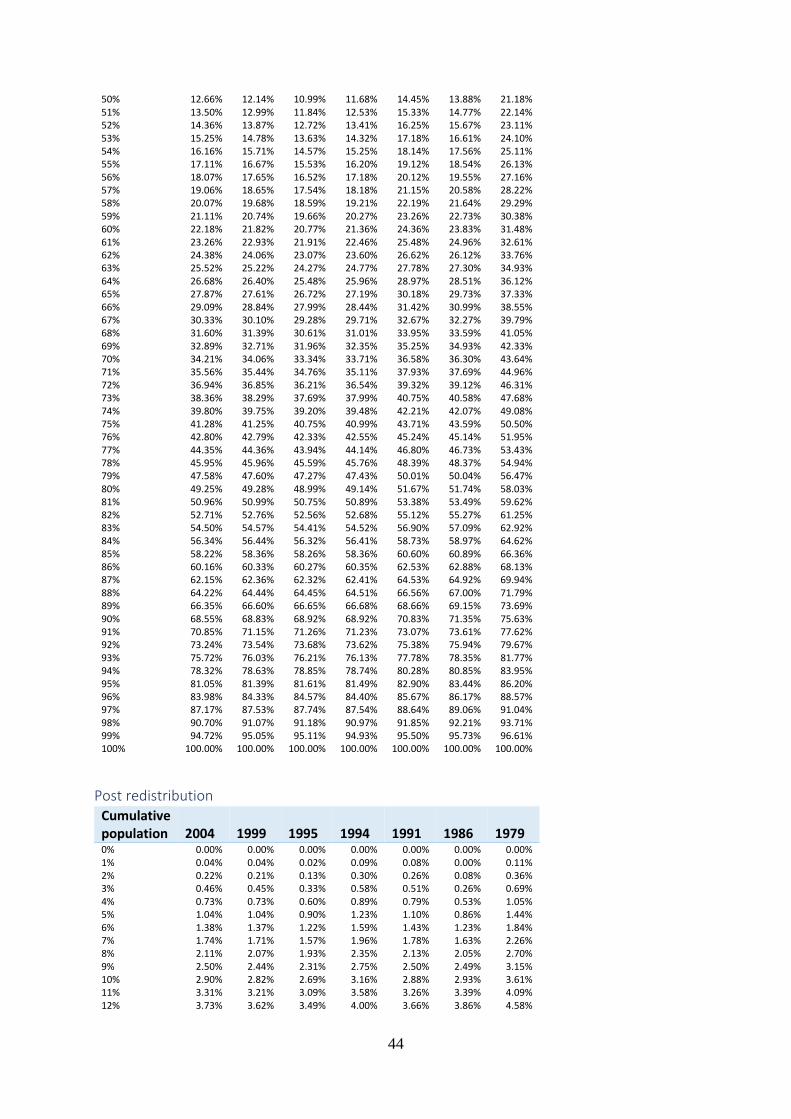
44

50% 12.66% 12.14% 10.99% 11.68% 14.45% 13.88% 21.18% 51% 13.50% 12.99% 11.84% 12.53% 15.33% 14.77% 22.14% 52% 14.36% 13.87% 12.72% 13.41% 16.25% 15.67% 23.11% 53% 15.25% 14.78% 13.63% 14.32% 17.18% 16.61% 24.10% 54% 16.16% 15.71% 14.57% 15.25% 18.14% 17.56% 25.11% 55% 17.11% 16.67% 15.53% 16.20% 19.12% 18.54% 26.13% 56% 18.07% 17.65% 16.52% 17.18% 20.12% 19.55% 27.16% 57% 19.06% 18.65% 17.54% 18.18% 21.15% 20.58% 28.22% 58% 20.07% 19.68% 18.59% 19.21% 22.19% 21.64% 29.29% 59% 21.11% 20.74% 19.66% 20.27% 23.26% 22.73% 30.38% 60% 22.18% 21.82% 20.77% 21.36% 24.36% 23.83% 31.48% 61% 23.26% 22.93% 21.91% 22.46% 25.48% 24.96% 32.61% 62% 24.38% 24.06% 23.07% 23.60% 26.62% 26.12% 33.76% 63% 25.52% 25.22% 24.27% 24.77% 27.78% 27.30% 34.93% 64% 26.68% 26.40% 25.48% 25.96% 28.97% 28.51% 36.12% 65% 27.87% 27.61% 26.72% 27.19% 30.18% 29.73% 37.33% 66% 29.09% 28.84% 27.99% 28.44% 31.42% 30.99% 38.55% 67% 30.33% 30.10% 29.28% 29.71% 32.67% 32.27% 39.79% 68% 31.60% 31.39% 30.61% 31.01% 33.95% 33.59% 41.05% 69% 32.89% 32.71% 31.96% 32.35% 35.25% 34.93% 42.33% 70% 34.21% 34.06% 33.34% 33.71% 36.58% 36.30% 43.64% 71% 35.56% 35.44% 34.76% 35.11% 37.93% 37.69% 44.96% 72% 36.94% 36.85% 36.21% 36.54% 39.32% 39.12% 46.31% 73% 38.36% 38.29% 37.69% 37.99% 40.75% 40.58% 47.68% 74% 39.80% 39.75% 39.20% 39.48% 42.21% 42.07% 49.08% 75% 41.28% 41.25% 40.75% 40.99% 43.71% 43.59% 50.50% 76% 42.80% 42.79% 42.33% 42.55% 45.24% 45.14% 51.95% 77% 44.35% 44.36% 43.94% 44.14% 46.80% 46.73% 53.43% 78% 45.95% 45.96% 45.59% 45.76% 48.39% 48.37% 54.94% 79% 47.58% 47.60% 47.27% 47.43% 50.01% 50.04% 56.47% 80% 49.25% 49.28% 48.99% 49.14% 51.67% 51.74% 58.03% 81% 50.96% 50.99% 50.75% 50.89% 53.38% 53.49% 59.62% 82% 52.71% 52.76% 52.56% 52.68% 55.12% 55.27% 61.25% 83% 54.50% 54.57% 54.41% 54.52% 56.90% 57.09% 62.92% 84% 56.34% 56.44% 56.32% 56.41% 58.73% 58.97% 64.62% 85% 58.22% 58.36% 58.26% 58.36% 60.60% 60.89% 66.36% 86% 60.16% 60.33% 60.27% 60.35% 62.53% 62.88% 68.13% 87% 62.15% 62.36% 62.32% 62.41% 64.53% 64.92% 69.94% 88% 64.22% 64.44% 64.45% 64.51% 66.56% 67.00% 71.79% 89% 66.35% 66.60% 66.65% 66.68% 68.66% 69.15% 73.69% 90% 68.55% 68.83% 68.92% 68.92% 70.83% 71.35% 75.63% 91% 70.85% 71.15% 71.26% 71.23% 73.07% 73.61% 77.62% 92% 73.24% 73.54% 73.68% 73.62% 75.38% 75.94% 79.67% 93% 75.72% 76.03% 76.21% 76.13% 77.78% 78.35% 81.77% 94% 78.32% 78.63% 78.85% 78.74% 80.28% 80.85% 83.95% 95% 81.05% 81.39% 81.61% 81.49% 82.90% 83.44% 86.20% 96% 83.98% 84.33% 84.57% 84.40% 85.67% 86.17% 88.57% 97% 87.17% 87.53% 87.74% 87.54% 88.64% 89.06% 91.04% 98% 90.70% 91.07% 91.18% 90.97% 91.85% 92.21% 93.71% 99% 94.72% 95.05% 95.11% 94.93% 95.50% 95.73% 96.61% 100% 100.00% 100.00% 100.00% 100.00% 100.00% 100.00% 100.00%

Post redistribution Cumulative population 2004 1999 1995 1994 1991 1986 1979 0% 0.00% 0.00% 0.00% 0.00% 0.00% 0.00% 0.00% 1% 0.04% 0.04% 0.02% 0.09% 0.08% 0.00% 0.11% 2% 0.22% 0.21% 0.13% 0.30% 0.26% 0.08% 0.36% 3% 0.46% 0.45% 0.33% 0.58% 0.51% 0.26% 0.69% 4% 0.73% 0.73% 0.60% 0.89% 0.79% 0.53% 1.05% 5% 1.04% 1.04% 0.90% 1.23% 1.10% 0.86% 1.44% 6% 1.38% 1.37% 1.22% 1.59% 1.43% 1.23% 1.84% 7% 1.74% 1.71% 1.57% 1.96% 1.78% 1.63% 2.26% 8% 2.11% 2.07% 1.93% 2.35% 2.13% 2.05% 2.70% 9% 2.50% 2.44% 2.31% 2.75% 2.50% 2.49% 3.15% 10% 2.90% 2.82% 2.69% 3.16% 2.88% 2.93% 3.61% 11% 3.31% 3.21% 3.09% 3.58% 3.26% 3.39% 4.09% 12% 3.73% 3.62% 3.49% 4.00% 3.66% 3.86% 4.58%

45

13% 4.16% 4.03% 3.91% 4.44% 4.08% 4.35% 5.07% 14% 4.60% 4.45% 4.33% 4.89% 4.50% 4.84% 5.58% 15% 5.06% 4.89% 4.77% 5.34% 4.93% 5.34% 6.11% 16% 5.52% 5.33% 5.21% 5.80% 5.37% 5.85% 6.64% 17% 5.99% 5.78% 5.67% 6.28% 5.82% 6.38% 7.19% 18% 6.48% 6.25% 6.13% 6.76% 6.28% 6.91% 7.74% 19% 6.97% 6.72% 6.61% 7.26% 6.74% 7.45% 8.31% 20% 7.48% 7.20% 7.09% 7.76% 7.22% 8.00% 8.89% 21% 7.99% 7.69% 7.59% 8.27% 7.71% 8.56% 9.49% 22% 8.52% 8.20% 8.10% 8.79% 8.22% 9.12% 10.09% 23% 9.05% 8.71% 8.61% 9.32% 8.73% 9.70% 10.71% 24% 9.60% 9.23% 9.14% 9.85% 9.25% 10.29% 11.34% 25% 10.15% 9.77% 9.67% 10.40% 9.79% 10.89% 11.99% 26% 10.72% 10.31% 10.22% 10.96% 10.33% 11.49% 12.64% 27% 11.29% 10.87% 10.77% 11.52% 10.89% 12.11% 13.31% 28% 11.87% 11.43% 11.33% 12.10% 11.46% 12.74% 13.98% 29% 12.47% 12.01% 11.91% 12.69% 12.05% 13.38% 14.67% 30% 13.07% 12.60% 12.50% 13.29% 12.65% 14.02% 15.37% 31% 13.68% 13.20% 13.09% 13.90% 13.25% 14.68% 16.08% 32% 14.31% 13.81% 13.71% 14.52% 13.88% 15.35% 16.80% 33% 14.94% 14.43% 14.34% 15.15% 14.51% 16.03% 17.53% 34% 15.59% 15.07% 14.98% 15.79% 15.16% 16.72% 18.27% 35% 16.25% 15.72% 15.63% 16.45% 15.82% 17.43% 19.02% 36% 16.91% 16.38% 16.29% 17.11% 16.49% 18.14% 19.79% 37% 17.59% 17.05% 16.97% 17.79% 17.18% 18.87% 20.56% 38% 18.28% 17.74% 17.65% 18.48% 17.88% 19.60% 21.35% 39% 18.98% 18.44% 18.35% 19.18% 18.60% 20.35% 22.15% 40% 19.70% 19.14% 19.05% 19.89% 19.33% 21.11% 22.96% 41% 20.42% 19.87% 19.77% 20.61% 20.07% 21.88% 23.78% 42% 21.16% 20.60% 20.51% 21.35% 20.83% 22.67% 24.61% 43% 21.91% 21.35% 21.25% 22.10% 21.60% 23.47% 25.45% 44% 22.68% 22.11% 22.02% 22.86% 22.38% 24.28% 26.29% 45% 23.45% 22.88% 22.80% 23.64% 23.17% 25.10% 27.15% 46% 24.24% 23.66% 23.59% 24.42% 23.98% 25.94% 28.02% 47% 25.03% 24.46% 24.40% 25.22% 24.80% 26.78% 28.91% 48% 25.84% 25.27% 25.22% 26.04% 25.64% 27.64% 29.80% 49% 26.66% 26.10% 26.05% 26.86% 26.49% 28.51% 30.71% 50% 27.50% 26.94% 26.90% 27.70% 27.35% 29.39% 31.62% 51% 28.34% 27.79% 27.76% 28.55% 28.23% 30.29% 32.55% 52% 29.20% 28.66% 28.64% 29.42% 29.12% 31.20% 33.49% 53% 30.07% 29.54% 29.54% 30.30% 30.03% 32.12% 34.43% 54% 30.95% 30.44% 30.44% 31.20% 30.95% 33.06% 35.39% 55% 31.85% 31.35% 31.36% 32.11% 31.88% 34.01% 36.37% 56% 32.76% 32.28% 32.30% 33.03% 32.82% 34.97% 37.35% 57% 33.69% 33.22% 33.25% 33.97% 33.79% 35.95% 38.35% 58% 34.63% 34.17% 34.21% 34.92% 34.77% 36.94% 39.37% 59% 35.58% 35.14% 35.20% 35.89% 35.76% 37.95% 40.39% 60% 36.55% 36.13% 36.20% 36.87% 36.77% 38.96% 41.43% 61% 37.54% 37.13% 37.21% 37.87% 37.79% 40.00% 42.47% 62% 38.53% 38.15% 38.24% 38.89% 38.83% 41.05% 43.53% 63% 39.55% 39.19% 39.29% 39.92% 39.88% 42.12% 44.60% 64% 40.58% 40.24% 40.36% 40.97% 40.95% 43.20% 45.69% 65% 41.63% 41.31% 41.44% 42.04% 42.05% 44.29% 46.79% 66% 42.69% 42.39% 42.54% 43.12% 43.15% 45.39% 47.91% 67% 43.77% 43.50% 43.66% 44.22% 44.28% 46.51% 49.03% 68% 44.87% 44.63% 44.80% 45.34% 45.42% 47.66% 50.18% 69% 45.98% 45.77% 45.95% 46.48% 46.58% 48.81% 51.34% 70% 47.12% 46.94% 47.12% 47.65% 47.76% 49.99% 52.51% 71% 48.27% 48.12% 48.31% 48.83% 48.97% 51.19% 53.71% 72% 49.44% 49.33% 49.53% 50.02% 50.19% 52.41% 54.92% 73% 50.64% 50.56% 50.76% 51.24% 51.44% 53.65% 56.15% 74% 51.85% 51.80% 52.02% 52.48% 52.71% 54.91% 57.39% 75% 53.09% 53.07% 53.30% 53.73% 54.00% 56.18% 58.66% 76% 54.35% 54.37% 54.60% 55.02% 55.32% 57.48% 59.94% 77% 55.63% 55.68% 55.92% 56.32% 56.66% 58.79% 61.24% 78% 56.94% 57.02% 57.26% 57.65% 58.02% 60.13% 62.56% 79% 58.28% 58.40% 58.62% 59.00% 59.42% 61.49% 63.90% 80% 59.63% 59.80% 60.01% 60.38% 60.84% 62.88% 65.26% 81% 61.02% 61.23% 61.42% 61.79% 62.29% 64.30% 66.64% 82% 62.44% 62.68% 62.86% 63.23% 63.77% 65.75% 68.03% 83% 63.89% 64.17% 64.33% 64.71% 65.28% 67.22% 69.45%

46

84% 65.38% 65.69% 65.85% 66.21% 66.83% 68.72% 70.89% 85% 66.91% 67.25% 67.39% 67.76% 68.41% 70.24% 72.36% 86% 68.47% 68.84% 68.98% 69.33% 70.02% 71.79% 73.86% 87% 70.08% 70.49% 70.60% 70.94% 71.67% 73.38% 75.38% 88% 71.74% 72.17% 72.28% 72.60% 73.35% 75.02% 76.93% 89% 73.44% 73.91% 74.01% 74.29% 75.08% 76.68% 78.51% 90% 75.20% 75.69% 75.77% 76.04% 76.85% 78.39% 80.13% 91% 77.01% 77.54% 77.60% 77.84% 78.66% 80.13% 81.79% 92% 78.90% 79.44% 79.47% 79.71% 80.53% 81.92% 83.49% 93% 80.85% 81.41% 81.42% 81.66% 82.48% 83.77% 85.23% 94% 82.90% 83.48% 83.46% 83.68% 84.49% 85.68% 87.02% 95% 85.05% 85.62% 85.61% 85.79% 86.58% 87.67% 88.88% 96% 87.35% 87.93% 87.91% 88.02% 88.78% 89.75% 90.81% 97% 89.84% 90.42% 90.35% 90.41% 91.10% 91.95% 92.83% 98% 92.58% 93.12% 92.98% 93.04% 93.65% 94.30% 94.96% 99% 95.77% 96.16% 96.04% 96.08% 96.51% 96.91% 97.30% 100% 100.00% 100.00% 100.00% 100.00% 100.00% 100.00% 100.00%