weather prediction by numerical process - ucd school of...

1

Weather Prediction by Numerical Process

Perhaps some day in the dim future it will be possible to advance thecomputations faster than the weather advances and at a cost less thanthe saving to mankind due to the information gained. But that is a dream.(WPNP, p. vii; Dover Edn., p. xi)

Lewis Fry Richardson’s extraordinary book Weather Prediction by Numerical Pro-cess, published in 1922, is a strikingly original scientific work, one of the mostremarkable books on meteorology ever written. In this book—to which we will re-fer briefly as WPNP—Richardson constructed a systematic mathematical methodfor predicting the weather and demonstrated its application by carrying out a trialforecast. History has shown that his innovative ideas were fundamentally sound:the methodology proposed by him is essentially that used in practical weather fore-casting today. However, the method devised by Richardson was utterly impracticalat the time of its publication and the results of his trial forecast appeared to belittle short of outlandish. As a result, his ideas were eclipsed for decades and hiswonderful opus gathered dust and was all but forgotten.

1.1 The problem

Imagine you are standing by the ocean shore, watching the sea rise and fall as waveupon wave breaks on the rocks. At a given moment the water is rising at a rate ofone metre per second—soon it will fall again. Is there an ebb or a flood tide?Suppose you use the observed rate of change and extrapolate it over the six hoursthat elapse between tidal extremes; you will obtain an extraordinary prediction:the water level should rise by some

��km, twice the height of Mt Everest. This

forecast is meaningless! The water level is governed by physical processes witha wide range of time-scales. The tidal variations, driven by lunar gravity, havea period of around twelve hours, linked to the Earth’s rotation. But wind-driven

1

2 Weather Prediction by Numerical Process

0 3 6 9 12 15 18 21 241008

1010

1012

1014

1016

1018

1020

1022 PRESSURE v. TIME

Fig. 1.1. Schematic illustration of pressure variation over a 24 hour period. The thick lineis the mean, long-term variation, the thin line is the actual pressure, with high frequencynoise. The dotted line shows the rate of change, at 12 hours, of the mean pressure and thedashed line shows the corresponding rate of change of the actual pressure (after Phillips,1973).

waves and swell vary on a time-scale of seconds. The instantaneous change inlevel due to a wave is no guide to the long-term tidal variations: if the observedrise is extrapolated over a period much longer than the time-scale of the wave, theresulting forecast will be calamitous.

In 1922 Richardson presented such a forecast to the world. He calculated achange of atmospheric pressure, for a particular place and time, of �� hPa in6 hours. This was a totally unrealistic value, too large by two orders of magni-tude. The prediction failed for reasons similar to those that destroy the hypothet-ical tidal forecast. The spectrum of motions in the atmosphere is analogous tothat of the ocean: there are long-period variations dominated by the effects of theEarth’s rotation—these are the meteorologically significant rotational modes—andshort-period oscillations called gravity waves, having speeds comparable to that ofsound. The interaction between the two types of variation is weak, just as is theinteraction between wind-waves and tidal motions in the ocean; and, for many pur-poses, the gravity waves, which are normally of small amplitude, may be treatedas irrelevant noise.

1.1 The problem 3

Although they have little effect on the long-term evolution of the flow, gravitywaves may profoundly influence the way it changes on shorter time-scales. Fig. 1.1(after Phillips, 1973) schematically depicts the pressure variation over a period ofone day. The smooth curve represents the variation due to meteorological effects;its gentle slope (dotted line) indicates the long-term change. The rapidly varyingcurve represents the actual pressure changes when gravity waves are superimposedon the meteorological flow: the slope of the oscillating curve (dashed line) is pre-cipitous and, if used to determine long-range variations, yields totally misleadingresults. What Richardson calculated was the instantaneous rate of change in pres-sure for an atmospheric state having gravity wave components of large amplitude.This tendency, ��

, was a sizeable but not impossible value. Suchvariations are observed over short periods in intense, localized weather systems.1

The problem arose when Richardson used the computed value in an attempt todeduce the long-term change. Multiplying the calculated tendency by a time stepof six hours, he obtained the unacceptable value quoted above. The cause of thefailure is this: the instantaneous pressure tendency does not reflect the long-termchange.

This situation looks hopeless: how are we to make a forecast if the tendenciescalculated using the basic equations of motion do not guide us? There are severalpossible ways out of the dilemma; their success depends crucially on the decou-pling between the gravity waves and the motions of meteorological significance—we can distort the former without seriously corrupting the latter.

The most obvious approach is to construct a forecast by combining many timesteps which are short enough to enable accurate simulation of the detailed high fre-quency variations depicted schematically in Fig. 1.1. The existence of these highfrequency solutions leads to a stringent limitation on the size of the time step foraccurate results; this limitation or stability criterion was discovered in a differentcontext by Hans Lewy in Gottingen in the 1920s (see Reid, 1976), and was firstpublished in Courant et al. (1928). Thus, although these oscillations are not ofmeteorological interest, their presence severely limits the range of applicability ofthe tendency calculated at the initial time. Small time steps are required to rep-resent the rapid variations and ensure accuracy of the long-term solution. If suchsmall steps are taken, the solution will contain gravity-wave oscillations about anessentially correct meteorological flow. One implication of this is that, if Richard-son could have extended his calculations, taking a large number of small steps, hisresults would have been noisy but the mean values would have been meteorolog-ically reasonable (Phillips, 1973). Of course, the attendant computational burdenmade this impossible for Richardson.

1 For example, Loehrer & Johnson (1995) reported a surface pressure drop of 4 hPa in five minutes in amesoscale convective system, or ��! ��#" $!%!&�')(+* .


The second approach is to modify the governing equations in such a way thatthe gravity waves no longer occur as solutions. This process is known as filteringthe equations. The approach is of great historical importance. The first successfulcomputer forecasts (Charney, et al., 1950) were made with the barotropic vorticityequation (see Ch. 10) which has low frequency but no high frequency solutions.Later, the quasi-geostrophic equations were used to construct more realistic filteredmodels and were used operationally for many years. An interesting account of thedevelopment of this system appeared in Phillips (1990). The quasi-geostrophicequations are still of great theoretical interest (Holton, 2004) but are no longerconsidered to be sufficiently accurate for numerical prediction.

The third approach is to adjust the initial data so as to reduce or eliminate thegravity wave components. The adjustments can be small in amplitude but largein effect. This process is called initialization, and it may be regarded as a formof smoothing. Richardson realized the requirement for smoothing the initial dataand devoted a chapter of WPNP to this topic. We will examine several methodsof initialization in this work, in particular in Chapter 8, and will show that thedigital filtering initialization method yields realistic tendencies when applied toRichardson’s data.

The absence of gravity waves from the initial data results in reasonable initialrates of change, but it does not automatically allow the use of large time steps.The existence of high frequency solutions of the governing equations imposes asevere restriction on the size of the time step allowable if reasonable results areto be obtained. The restriction can be circumvented by treating those terms ofthe equations that govern gravity waves in a numerically implicit manner; thisdistorts the structure of the gravity waves but not of the low frequency modes.In effect, implicit schemes slow down the faster waves thus removing the cause ofnumerical instability (see � 5.2 below). Most modern forecasting models avoid thepitfall that trapped Richardson by means of initialization followed by semi-implicitintegration.

1.2 Vilhelm Bjerknes and scientific forecasting

At the time of the First World War, weather forecasting was very imprecise andunreliable. Observations were scarce and irregular, especially for the upper air andover the oceans. The principles of theoretical physics played a relatively minorrole in practical forecasting: the forecaster used crude techniques of extrapolation,knowledge of climatology and guesswork based on intuition; forecasting was morean art than a science. The observations of pressure and other variables were plottedin symbolic form on a weather map and lines were drawn through points withequal pressure to reveal the pattern of weather systems—depressions, anticyclones,

1.2 Vilhelm Bjerknes and scientific forecasting 5

Fig. 1.2. A recent painting (from photographs) of the Norwegian scientist Vilhelm Bjerk-nes (1862–1951) standing on the quay in Bergen ( c

�Geophysical Institute, Bergen. Artist:

Rolf Groven).

troughs and ridges. The concept of fronts, surfaces of discontinuity between warmand cold airmasses, had yet to emerge. The forecaster used his experience, memoryof similar patterns in the past and a menagerie of empirical rules to produce aforecast map. Particular attention was paid to the reported pressure changes ortendencies; to a great extent it was assumed that what had been happening up tonow would continue for some time. The primary physical process attended to bythe forecaster was advection, the transport of fluid characteristics and properties bythe movement of the fluid itself.

The first explicit analysis of the weather prediction problem from a scientificviewpoint was undertaken at the beginning of the twentieth century when the Nor-wegian scientist Vilhelm Bjerknes set down a two-step plan for rational forecasting(Bjerknes, 1904):

If it is true, as every scientist believes, that subsequent atmospheric states de-velop from the preceding ones according to physical law, then it is apparent thatthe necessary and sufficient conditions for the rational solution of forecastingproblems are the following:


1. A sufficiently accurate knowledge of the state of the atmosphere at the initialtime.

2. A sufficiently accurate knowledge of the laws according to which one state of theatmosphere develops from another.

Bjerknes used the medical terms diagnostic and prognostic for these two steps(Friedman, 1989). The diagnostic step requires adequate observational data to de-fine the three-dimensional structure of the atmosphere at a particular time. Therewas a severe shortage of observations, particularly over the seas and for the upperair, but Bjerknes was optimistic:

We can hope . . . that the time will soon come when either as a daily routine, orfor certain designated days, a complete diagnosis of the state of the atmospherewill be available. The first condition for putting forecasting on a rational basiswill then be satisfied.

In fact, such designated days, on which upper air observations were made through-out Europe, were organised around that time by the International Commission forScientific Aeronautics.

The second or prognostic step was to be taken by assembling a set of equations,one for each dependent variable describing the atmosphere. Bjerknes listed sevenbasic variables: pressure, temperature, density, humidity and three components ofvelocity. He then identified seven independent equations: the three hydrodynamicequations of motion, the continuity equation, the equation of state and the equa-tions expressing the two laws of thermodynamics. (As pointed out by Eliassen(1999), Bjerknes was in error in listing the second law of thermodynamics; heshould instead have specified a continuity equation for water substance.) Bjerk-nes knew that an exact analytical integration was beyond our ability. His idea wasto represent the initial state of the atmosphere by a number of charts giving thedistribution of the variables at different levels. Graphical or mixed graphical andnumerical methods, based on the fundamental equations, could then be applied toconstruct a new set of charts describing the state of the atmosphere, say, three hourslater. This process could be repeated until the desired forecast length was reached.Bjerknes realized that the prognostic procedure could be conveniently separatedinto two stages, a purely hydrodynamic part and a purely thermodynamic part; thehydrodynamics would determine the movement of an airmass over the time inter-val and thermodynamic considerations could then be used to deduce changes in itsstate. He concluded:

It may be possible some day, perhaps, to utilise a method of this kind as the basisfor a daily practical weather service. But however that may be, the fundamentalscientific study of atmospheric processes sooner or later has to follow a methodbased upon the laws of mechanics and physics.

Bjerknes’ speculations are reminiscent of Richardson’s ‘dream’ of practical scien-tific weather forecasting.


Fig. 1.3. Top: Exner’s calculated pressure change between 8 p.m. and midnight, 3 January,1895. Bottom: Observed pressure change for the same period [Units: Hundreths of an inchof mercury. Steigt=rises; Fallt=falls] (Exner, 1908).

A tentative first attempt at mathematically forecasting synoptic changes by theapplication of physical principles was made by Felix Exner, working in Vienna.His account (Exner, 1908) appeared only four years after Bjerknes’ seminal paper.Exner makes no reference to Bjerknes’ work, which was also published in Meteo-


rologische Zeitschrift. Though he may be presumed to have known about Bjerknes’ideas, Exner followed a radically different line: whereas Bjerknes proposed thatthe full system of hydrodynamic and thermodynamic equations be used, Exner’smethod was based on a system reduced to the essentials. He assumed that the atmo-spheric flow is geostrophically balanced and that the thermal forcing is constant intime. Using observed temperature values, he deduced a mean zonal wind. He thenderived a prediction equation representing advection of the pressure pattern withconstant westerly speed, modified by the effects of diabatic heating. It yielded a re-alistic forecast in the case illustrated in Exner’s paper. Fig. 1.3 shows his calculatedpressure change (top) and the observed change (bottom) over the four hour periodbetween 8 p.m. and midnight on 3 January, 1895; there is reasonable agreementbetween the predicted and observed changes. However, the method could hardlybe expected to be of general utility. Exner took pains to stress the limitations ofhis method, making no extravagant claims for it. But despite the very restrictedapplicability of the technique devised by him, the work is deserving of attentionas a first attempt at systematic, scientific weather forecasting. Exner’s numericalmethod was summarized in his textbook (Exner, 1917, � 70). The only reference byRichardson to the method was a single sentence (WPNP, p. 43) ‘F. M. Exner haspublished a prognostic method based on the source of air supply.’ It would appearfrom this that Richardson was not particularly impressed by it!

In 1912 Bjerknes became the first Director of the new Geophysical Institute inLeipzig. In his inaugural lecture he returned to the theme of scientific forecasting.He observed that ‘physics ranks among the so-called exact sciences, while one maybe tempted to cite meteorology as an example of a radically inexact science.’ Hecontrasted the methods of meteorology with those of astronomy, for which predic-tions of great accuracy are possible, and described the programme of work uponwhich he had already embarked: to make meteorology into an exact physics of theatmosphere. Considerable advances had been made in observational meteorologyduring the previous decade, so that now the diagnostic component of his two-stepprogramme had become feasible.

. . . now that complete observations from an extensive portion of the free air arebeing published in a regular series, a mighty problem looms before us and we canno longer disregard it. We must apply the equations of theoretical physics notto ideal cases only, but to the actual existing atmospheric conditions as they arerevealed by modern observations. These equations contain the laws according towhich subsequent atmospheric conditions develop from those that precede them.It is for us to discover a method of practically utilising the knowledge containedin the equations. From the conditions revealed by the observations we must learnto compute those that will follow. The problem of accurate pre-calculation thatwas solved for astronomy centuries ago must now be attacked in all ernest formeteorology (Bjerknes, 1914a).

Bjerknes expressed his conviction that the acid test of a science is its utility in fore-


casting: ‘There is after all but one problem worth attacking, viz., the precalculationof future conditions.’ He recognised the complexity of the problem and realizedthat a rational forecasting procedure might require more time than the atmosphereitself takes to evolve, but concluded:

If only the calculation shall agree with the facts, the scientific victory will bewon. Meteorology would then have become an exact science, a true physics ofthe atmosphere. When that point is reached, then the practical results will soondevelop.

It may require many years to bore a tunnel through a mountain. Many alabourer may not live to see the cut finished. Nevertheless this will not preventlater comers from riding through the tunnel at express-train speed.

At Leipzig Bjerknes instigated the publication of a series of weather charts basedon the data that were collected during the internationally-agreed intensive obser-vation days and compiled and published by Hugo Hergesell in Strasbourg (thesecharts are discussed in detail in Chapter 6 below). One such publication (Bjerknes,1914b), together with the ‘raw data’ in Hergesell (1913), was to provide Richard-son with the initial conditions for his forecast.

Richardson first heard of Bjerknes’ plan for rational forecasting in 1913, whenhe took up employment with the Meteorological Office. In the Preface to WPNPhe writes

The extensive researches of V. Bjerknes and his School are pervaded by the ideaof using the differential equations for all that they are worth. I read his volumeson Statics and Kinematics soon after beginning the present study, and they haveexercised a considerable influence throughout it.

Richardson’s book opens with a discussion of then-current practice in the Met Of-fice. He describes the use of an Index of Weather Maps, constructed by classifyingold synoptic charts into categories. The Index (Gold, 1919) assisted the forecasterto find previous maps resembling the current one and therewith to deduce the likelydevelopment by studying the evolution of these earlier cases:

The forecast is based on the supposition that what the atmosphere did then, itwill do again now. There is no troublesome calculation, with its possibilities oftheoretical or arithmetical error. The past history of the atmosphere is used, soto speak, as a full-scale working model of its present self (WPNP, p. vii; DoverEdn., p. xi).

Bjerknes had contrasted the precision of astronomical prediction with the ‘radicallyinexact’ methods of weather forecasting. Richardson returned to this theme in hisPreface:

—the Nautical Almanac, that marvel of accurate forecasting, is not based onthe principle that astronomical history repeats itself in the aggregate. It wouldbe safe to say that a particular disposition of stars, planets and satellites neveroccurs twice. Why then should we expect a present weather map to be exactlyrepresented in a catalogue of past weather? . . . This alone is sufficient reasonfor presenting, in this book, a scheme of weather prediction which resemblesthe process by which the Nautical Almanac is produced, in so far as it is founded


upon the differential equations and not upon the partial recurrence of phenomenain their ensemble.

Richardson’s forecasting scheme amounts to a precise and detailed implementationof the prognostic component of Bjerknes’ programme. It is a highly intricate proce-dure: as Richardson observed, ‘the scheme is complicated because the atmosphereis complicated.’ It also involved an enormous volume of numerical computationand was quite impractical in the pre-computer era. But Richardson was undaunted,expressing his dream that ‘some day in the dim future it will be possible to advancethe computations faster than the weather advances’. Today, forecasts are preparedroutinely on powerful computers running algorithms that are remarkably similar toRichardson’s scheme — his dream has indeed come true.

Before discussing Richardson’s forecast in more detail, we will digress brieflyto consider his life and work from a more general viewpoint.

1.3 Outline of Richardson’s life and work

Richardson’s life and work are discussed in a comprehensive and readable biogra-phy (Ashford, 1985). The Royal Society Memoir of Gold (1954) provides a moresuccinct description and the Collected Papers of Richardson, edited by Drazin(LFR I) and Sutherland (LFR II), include a biographical essay by Hunt (1993);see also Hunt (1998). Brief introductions to Richardson’s work in meteorology(by Henry Charnock), in numerical analysis (by Leslie Fox) and on fractals (byPhilip Drazin) are also included in Volume 1 of the Collected Papers. The articleby Chapman (1965) is worthy of attention and some fascinating historical back-ground material may be found in the review by Platzman (1967). In a recent popu-lar book on mathematics, Korner (1996) devotes two chapters (69 pages) to variousaspects of Richardson’s mathematical work. The National Cataloguing Unit for theArchives of Contemporary Scientists has produced a comprehensive catalogue ofthe papers and correspondence of Richardson, which were deposited by OliverAshford in Cambridge University Library (NCUACS, 1993). The following sketchof Richardson’s life is based primarily on Ashford’s book.

Lewis Fry Richardson was born in 1881, the youngest of seven children of DavidRichardson and Catherine Fry, both of whose families had been members of the So-ciety of Friends for generations. He was educated at Bootham, the Quaker schoolin York, where he showed an early aptitude for mathematics, and at Durham Col-lege of Science in Newcastle. He entered King’s College, Cambridge in 1900 andgraduated with a First Class Honours in the Natural Science Tripos in 1903. In1909 he married Dorothy Garnett. They had no offspring but adopted two sons anda daughter, Olaf (1916–1983), Stephen (b. 1920) and Elaine (b. 1927).

Over the ten years following his graduation, Richardson held several short re-

1.3 Outline of Richardson’s life and work 11

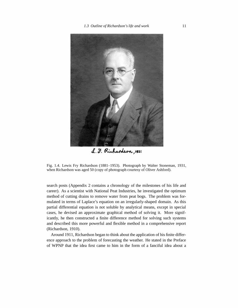
Fig. 1.4. Lewis Fry Richardson (1881–1953). Photograph by Walter Stoneman, 1931,when Richardson was aged 50 (copy of photograph courtesy of Oliver Ashford).

search posts (Appendix 2 contains a chronology of the milestones of his life andcareer). As a scientist with National Peat Industries, he investigated the optimummethod of cutting drains to remove water from peat bogs. The problem was for-mulated in terms of Laplace’s equation on an irregularly-shaped domain. As thispartial differential equation is not soluble by analytical means, except in specialcases, he devised an approximate graphical method of solving it. More signif-icantly, he then constructed a finite difference method for solving such systemsand described this more powerful and flexible method in a comprehensive report(Richardson, 1910).

Around 1911, Richardson began to think about the application of his finite differ-ence approach to the problem of forecasting the weather. He stated in the Prefaceof WPNP that the idea first came to him in the form of a fanciful idea about a


forecast factory, to which we will return in the final chapter. Richardson beganserious work on weather prediction in 1913 when he joined the Met Office and wasappointed Superintendent of Eskdalemuir Observatory, at an isolated location inDumfrieshire in the Southern Uplands of Scotland. In May 1916 he resigned fromthe Met Office in order to work with the Friends Ambulance Unit (FAU) in France.There he spent over two years as an ambulance driver, working in close proxim-ity to the fighting and on occasions coming under heavy shell fire. He returned toEngland after the cessation of hostilities and was employed once again by the MetOffice to work at Benson, between Reading and Oxford, with W. H. Dines. Theconditions of his employment included experiments with a view to forecasting bynumerical process. He also developed several ingenious instruments for makingupper air observations. However, he was there only one year when the Office cameunder the authority of the Air Ministry, which also had responsibility for the RoyalAir Force and, as a committed pacifist, he felt obliged to resign once more.

Richardson then obtained a post as a lecturer in mathematics and physics atWestminister Training College in London. His meteorological research now fo-cussed primarily on atmospheric turbulence. Several of his publications duringthis period are still cited by scientists. In one of the most important — The supplyof energy from and to atmospheric eddies (Richardson, 1920) — he derived a crite-rion for the onset of turbulence, introducing what is now known as the RichardsonNumber. In another, he investigated the separation of initially proximate tracersin a turbulent flow, and arrived empirically at his ‘four-thirds law’: the rate of dif-fusion is proportional to the separation raised to the power 4/3. This was laterestablished more rigourously by Kolmogorov (1941) using dimensional analysis.Bachelor (1950) showed the consistency between Richardson’s four-thirds law andKolmogorov’s similarity theory. A simple derivation of the four-thirds law usingdimensional analysis is given by Korner (1996).

In 1926 Richardson was elected a Fellow of the Royal Society. Around that timehe made a deliberate break with meteorological research. He was distressed thathis turbulence research was being exploited for military purposes. Moreover, hehad taken a degree in psychology and wanted to apply his mathematical knowl-edge in that field. Among his interests was the quantitative measurement of humansensation such as the perception of colour. He established for the first time a log-arithmic relationship between the perceived loudness and the physical intensity ofa stimulus. In 1929 he was appointed Principal of Paisley Technical College, nearGlasgow, and he worked there until his retirement in 1940.

From about 1935 until his death in 1953, Richardson thrust himself energeticallyinto peace studies, developing mathematical theories of human conflict and thecauses of war. Once again he produced ideas and results of startling originality. Hepioneered the application of quantitative methods in this extraordinarily difficult

1.3 Outline of Richardson’s life and work 13

area. As with his work in numerical weather prediction, the value of his effortswas not immediately appreciated. He produced two books, Arms and Insecurity(1947), a mathematical theory of arms races, and Statistics of Deadly Quarrels(1950) in which he amassed data on all wars and conflicts between 1820 and 1949in a systematic collection. His aim was to identify and understand the causes ofwar, with the ultimate humanitarian goal of preventing unnecessary waste of life.However, he was unsuccessful in finding a publisher for these books (the datesrefer to the original microfilm editions). The books were eventually publishedposthumously in 1960, thanks to the efforts of Richardson’s son Stephen. Thesestudies continue to be a rich source of ideas. A recent review of Richardson’stheories of war and peace has been written by Hess (1995).

Richardson’s genius was to apply quantitative methods to problems that hadtraditionally been regarded as beyond ‘mathematicization’, and the continuing rel-evance and usefulness of his work confirms the value of his ideas. He generallyworked in isolation, moving frequently from one subject to another. He lackedconstructive collaboration with colleagues and, perhaps as a result, his work hadgreat individuality but was also somewhat idiosyncratic. G. I. Taylor (1959) spokeof him as ‘a very interesting and original character who seldom thought on thesame lines as his contemporaries and often was not understood by them’. Just asfor his work in meteorology, Richardson’s mathematical studies of the causes ofwar were ahead of their time. In a letter to Nature (Richardson, 1951) he posedthe question of whether an arms race must necessarily lead to warfare. Reviewingthis work, his biographer (Ashford, 1985, p. 223) wrote ‘Let us hope that beforelong history will show that an arms race can indeed end without fighting.’ Just fouryears later the collapse of the Soviet Union brought the nuclear arms race to anabrupt end.2

Richardson’s Quaker background and pacifist convictions profoundly influencedthe course of his career. Late in his life, he wrote of the ‘persistent influence of theSociety of Friends, with its solemn emphasis on public and private duty’. Becauseof his pacifist principles, he resigned twice from the Met Office, first to face battle-field dangers in the Friends Ambulance Unit in France and again when the Officecame under the Air Ministry. He destroyed some of his research results to preventtheir use for military purposes (Brunt, 1954) and even ceased meteorological re-search for a time: he published no papers in meteorology between 1930 and 1948.He retired early on a meagre pension to devote all his energies to peace studies. Hiswork was misunderstood by many but his conviction and vision gave him courageto persist in the face of the indifference and occasional ridicule of his contempo-raries.

2 Stommel (1985) noted that the only purchaser of the book Arms and Insecurity, which Richardson was offeringfor sale on microfilm in 1948, was the Soviet Embassy in London!


Richardson made important contributions in several fields, the most importantbeing atmospheric diffusion, numerical analysis, quantitative psychology and themathematical study of the causes of war. He is remembered by meteorologiststhrough the Richardson Number, a fundamental quantity in turbulence theory, andfor his extraordinary vision in formulating the process of numerical forecasting.The approximate methods that he developed for the solution of differential equa-tions are extensively used in the numerical treatment of physical problems.

Richardson’s pioneering work in studying the mathematical basis of human con-flict has led to the establishment of a large number of university departments de-voted to this area. In the course of his peace studies, he digressed to consider thelengths of geographical borders and coastlines, and discovered the scaling proper-ties such that the length increases as the unit of measurement is reduced. This workinspired Benoit Mandelbrot’s development of the theory of fractals (Mandelbrot,1982). In a tribute to Richardson shortly after his death, his wife Dorothy recalledthat one of his sayings was ‘Our job in life is to make things better for those whofollow us. What happens to ourselves afterwards is not our concern.’ Richardsonhad the privilege to make contributions to human advancement in several areas.The lasting value of his work is a testimony of his wish to serve his fellow man.

1.4 The origin of Weather Prediction by Numerical Process

Richardson first applied his approximate method for the solution of differentialequations to investigate the stresses in masonry dams (Richardson, 1910), a prob-lem on which he had earlier worked with the statistician Karl Pearson. But themethod was completely general and he realized that it had potential for use in awide range of problems. The idea of numerical weather prediction appears to havegerminated in his mind for several years. In a letter to Pearson dated 6 April 1907he wrote in reference to the method that ‘there should be applications to meteorol-ogy one would think’ (Ashford, 1985, p. 25). This is the first inkling of his interestin the subject. In the Preface to WPNP he wrote that the investigation of numericalprediction

grew out of a study of finite differences and first took shape in 1911 as the fantasywhich is now relegated to Ch. 11/2. Serious attention to the problem was begunin 1913 at Eskdalemuir Observatory, with the permission and encouragement ofSir Napier Shaw, then Director of the Met Office, to whom I am greatly indebtedfor facilities, information and ideas.

The fantasy was that of a forecast factory, which we will discuss in detail in thefinal chapter. Richardson had had little or no previous experience of meteorologywhen he took up his position as Superintendent of the Observatory in what Gold(1954) described as ‘the bleak and humid solitude of Eskdalemuir’. Perhaps it wasthis lack of formal training in the subject that enabled him to approach the prob-

1.4 The origin of Weather Prediction by Numerical Process 15

Fig. 1.5. Eskdalemuir Observatory in 1911. Office and Computing Room, where Richard-son’s dream began to take shape (Photograph from MC-1911).

lem of weather forecasting from such a breathtakingly original and unconventionalangle. His plan was to express the physical principles that govern the behaviourof the atmosphere as a system of mathematical equations and to solve this systemusing his approximate finite difference method. The basic equations had alreadybeen identified by Bjerknes (1904) but with the error noted above: the secondlaw of thermodynamics was specified instead of conservation of water substance.The same error was repeated in Bjerknes’ inaugural address at Leipzig (Bjerknes,1914a). While this may seem a minor matter it proves that, while Bjerknes outlineda general philosophical approach, he did not attempt to formulate a detailed proce-dure, or algorithm, for applying his method. Indeed, he felt that such an approachwas completely impractical. The complete system of fundamental equations was,for the first time, set down in a systematic way in Ch. 4 of WPNP. The equationshad to be simplified, using the hydrostatic assumption, and transformed to renderthem amenable to approximate solution. Richardson also introduced a plethora ofextra terms to account for various physical processes not considered by Bjerknes.

By the time of his resignation in 1916, Richardson had completed the formu-lation of his scheme and had set down the details in the first draft of his book,then called Weather Prediction by Arithmetic Finite Differences. But he was not


concerned merely with theoretical rigour and wished to include a fully workedexample to demonstrate how the method could be put to use. This example

was worked out in France in the intervals of transporting wounded in 1916–1918.During the battle of Champagne in April 1917 the working copy was sent to therear, where it became lost, to be re-discovered some months later under a heapof coal (WPNP, p. ix; Dover Edn., p. xiii).

One may easily imagine Richardson’s distress at this loss and the great relief thatthe re-discovery must have brought him.3 It is a source of wonder that in the ap-palling conditions prevailing at the front he had the buoyancy of spirit to carry outone of the most remarkable and prodigious feats of calculation ever accomplished.

Richardson assumed that the state of the atmosphere at any point could be spec-ified by seven numbers: pressure, temperature, density, water content and velocitycomponents eastward, northward and upward. He formulated a description of at-mospheric phenomena in terms of seven differential equations. To solve them,Richardson divided the atmosphere into discrete columns of extent 3 � east-westand 200 km north-south, giving � �� columns to cover the globe.Each of these columns was divided vertically into five cells. The values of thevariables were given at the centre of each cell, and the differential equations wereapproximated by expressing them in finite difference form. The rates of changeof the variables could then be calculated by arithmetical means. Richardson calcu-lated the initial changes in two columns over central Europe, one for mass variablesand one for winds. This was the extent of his ‘forecast’.

How long did it take Richardson to make his forecast? It is generally believedthat he took six weeks for the task but, given the volume of results presented onhis 23 computing forms, it is difficult to understand how the work could have beenexpedited in so short a time. The question was discussed in Lynch (1993), whichis reproduced in Appendix 4. The answer is contained in � 11/2 of WPNP, but isexpressed in a manner that has led to confusion. On page 219, under the heading‘The Speed and Organization of Computing’, Richardson wrote

It took me the best part of six weeks to draw up the computing forms and to workout the new distribution in two vertical columns for the first time. My officewas a heap of hay in a cold rest billet. With practice the work of an averagecomputer might go perhaps ten times faster. If the time-step were 3 hours, then32 individuals could just compute two points so as to keep pace with the weather.

Could Richardson really have completed his task in six weeks? Given that 32computers4 working at ten times his speed would require 3 hours for the job, hehimself must have taken some 960 hours — that is 40 days or ‘the best part ofsix weeks’ working flat-out at 24 hours a day! At a civilized 40-hour week theforecast would have extended over six months. It is more likely that Richardson

3 In an obituary notice, Brunt (1954) stated that the manuscript was lost not once but twice.4 Richardson’s ‘computers’ were made not of silicon but of flesh and blood.

1.4 The origin of Weather Prediction by Numerical Process 17

spent perhaps ten hours per week at his chore and that it occupied him for abouttwo years, the greater part of his stay in France.

In 1919 Richardson added an introductory example (WPNP, Ch 2) in which heintegrated a system equivalent to the linearized shallow water equations, startingfrom idealised initial conditions defined by a simple analytic formula. This wasdone at Benson where he had ‘the good fortune to be able to discuss the hypotheseswith Mr W. H. Dines’. The chapter ends with an acknowledgement to Dines forhaving read and criticised it. It seems probable that the inclusion of this examplewas suggested by Dines, who might have been more sensitive than Richardsonto the difficulties that readers of WPNP would likely experience. The book wasthoroughly revised in 1920–21 and was finally published by Cambridge UniversityPress in 1922 at a price of 30 shillings (£1.50), the print run being 750 copies.

Richardson’s book was certainly not a commercial success. Akira Kasahara hastold me that he bought a copy from Cambridge University Press in 1955, more thanthirty years after publication. The book was re-issued in 1965 as a Dover paperbackand the 3,000 copies, priced at $2, about the same as the original hard-back edition,were sold out within a decade. The Dover edition was identical to the originalexcept for a six-page introduction by Sydney Chapman. Following its appearance,a retrospective appraisal of Richardson’s work by George Platzman was publishedin the Bulletin of the American Meteorological Society (Platzman, 1967; 1968).This scholarly review has been of immense assistance in the preparation of thepresent work.

The initial response to WPNP was unremarkable and must have been disap-pointing to Richardson. The book was widely reviewed with generally favourablecomments—Ashford (1985) includes a good coverage of reactions—but the im-practicality of the method and the abysmal failure of the solitary sample forecastinevitably attracted adverse criticism. Napier Shaw, reviewing the book for Na-ture, wrote that Richardson ‘presents to us a magnum opus on weather prediction’.However, in regard to the forecast, he observed that the wildest guess at the pressurechange would not have been wider of the mark. More importantly for our purposes,he questioned Richardson’s conclusion that wind observations were the real causeof the error, and also his dismissal of the geostrophic wind. Edgar W. Woolard, ameteorologist with the U.S. Weather Bureau, wrote

The book is an admirable study of an eminently important problem . . . a firstattempt in this extraordinarily difficult and complex field . . . it indicates a lineof attack on the problem, and invites further study with a view to improvementand extension. . . . It is sincerely to be hoped that the author will continue hisexcellent work along these lines, and that other investigators will be attracted tothe field which he has opened up. The results cannot fail to be of direct practicalimportance as well as of immense scientific value.

However, other investigators were not attracted to the field, perhaps because the


forecast failure acted as a deterrent, perhaps because the book was so difficult toread, with its encyclopædic but distracting range of topics. Alexander McAdie,Professor of Meteorology at Harvard, wrote ‘It can have but a limited number ofreaders and will probably be quickly placed on a library shelf and allowed to restundisturbed by most of those who purchase a copy’ (McAdie, 1923). Indeed, thisis essentially what happened to the book.

A most perceptive review by F. J. W. Whipple of the Met Office came closest tounderstanding Richardson’s unrealistic forecast, postulating that rapidly-travellingwaves contributed to its failure:

The trouble that he meets is that quite small discrepancies in the estimate of thestrengths of the winds may lead to comparatively large errors in the computedchanges of pressure. It is very doubtful whether sufficiently accurate results willever be arrived at by the straightforward application of the principle of conserva-tion of matter. In nature any excess of air in one place originates waves which arepropagated with the velocity of sound, and therefore much faster than ordinarymeteorological phenomena.

One of the difficulties in the mathematical analysis of pressure changes onthe Earth is that the great rapidity of these adjustments by the elasticity of the airhas to be allowed for. The difficulty does not crop up explicitly in Mr Richard-son’s work, but it may contribute to the failure of his method when he comes toclose quarters with a numerical problem.

The hydrostatic approximation used by Richardson eliminates vertically propagat-ing sound waves, but gravity waves and also horizontally propagating sound waves(Lamb waves) are present as solutions of his equations. These do indeed travel‘much faster than ordinary meteorological phenomena’. Nowhere in his book doesRichardson allude to this fact. Whipple appears to have had a far clearer under-standing of the causes of Richardson’s forecast catastrophe that did Richardsonhimself. The consideration of these causes is a central theme of the present work.

A humourist has observed that publishing a book of verse is like dropping afeather down the Grand Canyon and awaiting the echo. Richardson’s work was nottaken seriously and his book failed to have any significant impact on the practiceof meteorology during the decades following its publication. But the echo finallyarrived and continues to resound around the world to this day: Richardson’s bril-liant and prescient ideas are now universally recognised among meteorologists andhis work is the foundation upon which modern forecasting is built.

1.5 Outline of the contents of WPNP

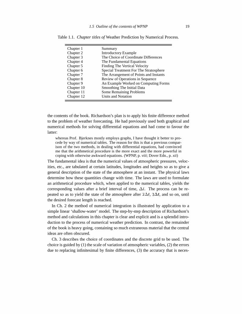
We will examine Richardson’s numerical forecast in considerable detail in thechapters that follow. For now, it is useful to present a broad outline — a synopticview — of his book. The chapter titles are given in Table 1.1. Ch. 1 is a summary of

1.5 Outline of the contents of WPNP 19

Table 1.1. Chapter titles of Weather Prediction by Numerical Process.

Chapter 1 SummaryChapter 2 Introductory ExampleChapter 3 The Choice of Coordinate DifferencesChapter 4 The Fundamental EquationsChapter 5 Finding The Vertical VelocityChapter 6 Special Treatment For The StratosphereChapter 7 The Arrangement of Points and InstantsChapter 8 Review of Operations in SequenceChapter 9 An Example Worked on Computing FormsChapter 10 Smoothing The Initial DataChapter 11 Some Remaining ProblemsChapter 12 Units and Notation

the contents of the book. Richardson’s plan is to apply his finite difference methodto the problem of weather forecasting. He had previously used both graphical andnumerical methods for solving differential equations and had come to favour thelatter:

whereas Prof. Bjerknes mostly employs graphs, I have thought it better to pro-cede by way of numerical tables. The reason for this is that a previous compar-ison of the two methods, in dealing with differential equations, had convincedme that the arithmetical procedure is the more exact and the more powerful incoping with otherwise awkward equations. (WPNP, p. viii; Dover Edn., p. xii)

The fundamental idea is that the numerical values of atmospheric pressures, veloc-ities, etc., are tabulated at certain latitudes, longitudes and heights so as to give ageneral description of the state of the atmosphere at an instant. The physical lawsdetermine how these quantities change with time. The laws are used to formulatean arithmetical procedure which, when applied to the numerical tables, yields thecorresponding values after a brief interval of time,

� � . The process can be re-peated so as to yield the state of the atmosphere after

� � � , �� , and so on, until

the desired forecast length is reached.In Ch. 2 the method of numerical integration is illustrated by application to a

simple linear ‘shallow-water’ model. The step-by-step description of Richardson’smethod and calculations in this chapter is clear and explicit and is a splendid intro-duction to the process of numerical weather prediction. In contrast, the remainderof the book is heavy going, containing so much extraneous material that the centralideas are often obscured.

Ch. 3 describes the choice of coordinates and the discrete grid to be used. Thechoice is guided by (1) the scale of variation of atmospheric variables, (2) the errorsdue to replacing infinitesimal by finite differences, (3) the accuracy that is neces-


sary to satisfy public requirements, (4) the cost, which increases with the numberof points in space and time that have to be dealt with’ (WPNP, p. 16). Richardsonconsidered the distribution of observing stations in the British Isles, which wereseparated, on average, by a distance of 130 km. Over the oceans, observations were‘scarce and irregular’. He concluded that a grid with 128 equally spaced meridiansand 200 km in latitude would be a reasonable choice. In the vertical he chose fivelayers, or conventional strata, separated by horizontal surfaces at 2.0, 4.2, 7.2 and11.8 km, corresponding approximately to the mean heights of the 800, 600, 400and 200 hPa surfaces. The alternative of using isobaric coordinates was consideredbut dismissed. The time interval chosen by Richardson was six hours, but this cor-responds to

� � � for the leapfrog method of integration; in modern terms, we have� � � �� . The cells of the horizontal grid were coloured alternately red and white,like the checkers of a chess-board. The grid was illustrated on the frontispiece ofWPNP, reproduced in Fig. 1.6.5

The next three chapters, comprising half the book, are devoted to assembling asystem of equations suitable for Richardson’s purposes. In Ch. 4

the fundamental equations are collected from various sources, set in order andcompleted where necessary. Those for the atmosphere are then integrated withrespect to height so as to make them apply to the mean values of the pressure,density, velocity, etc., in the several conventional strata.

As hydrostatic balance is assumed, there is no prognostic equation for the verticalvelocity. Ch. 5 is devoted to the derivation of a diagnostic equation for this quantity.Platzman (1967) wrote that Richardson’s vertical velocity equation ‘is the princi-pal, substantive contribution of the book to dynamic meteorology.’ Ch. 6 considersthe special measures which must be taken for the uppermost layer, the stratosphere,a region later described as ‘a happy hunting-ground for meteorological theorists’(Richardson and Munday, 1926).

Ch. 7 gives details of the finite difference scheme, explaining the rationale forthe choice of a staggered grid. Richardson considers several possible time-steppingtechniques, including a fully implicit scheme, but opts for the simple leapfrog or‘step-over’ method. Here can also be found a discussion of variable grid resolutionand the special treatment of the polar caps. In Ch. 8 the forecasting ‘algorithm’ ispresented in detail. It is carefully constructed so as to be, in Richardson’s words,lattice reproducing; that is, where a quantity is known at a particular time andplace, the algorithm enables its value at a later time to be calculated at the sameplace. The description of the method is sufficiently detailed and precise to enablea computer program based on it to be written, so that Richardson’s results can bereplicated (without the toil of two year’s manual calculation).

5 Richardson used 120 meridians, giving a 3 � east-west distance, for his actual forecast, later realizing that 128meridians (or � " � � �� ) would more conveniently facilitate sub-division near the poles.


Fig. 1.6. Richardson’s idealized computational grid (Frontispiece of WPNP).

Ch. 9 describes the celebrated trial forecast and its unfortunate results. Thepreparation of the initial data is outlined—the data are tabulated on page 185 ofWPNP. The calculations themselves are presented on a set of 23 Computer Forms.These were completed manually: ‘multiplications were mostly worked by a 25centim slide rule’ (WPNP, p. 186). The calculated changes in the primary variables


over a six hour period are compiled on page 211. It is characteristic of Richardson’swhimsical sense of humour that, on the heading of this page, the word “prediction”is enclosed in quotes; the results certainly cannot be taken literally. Richardsonexplains the chief result thus:

The rate of rise of surface pressure, �� , is found on Form �� as 145millibars in 6 hours, whereas observations show that the barometer was nearlysteady. This glaring error is examined in detail below in Ch. 9/3, and is traced toerrors in the representation of the initial winds.

(Here, �� is the surface pressure). Richardson described his forecast as ‘a fairlycorrect deduction from a somewhat unnatural initial distribution’ (WPNP, p. 211).We will consider this surprising claim in detail in the ensuing chapters.

The following chapter is given short shrift by Richardson in his summary: ‘InCh. 10 the smoothing of observations is discussed.’ The brevity of this resumeshould not be taken to reflect the status of the chapter. In its three pages, Richardsondiscusses five alternative smoothing techniques. Such methods are crucial for thesuccess of modern computer forecasting models. In a sense, Ch. 10 contains thekey to solving the difficulties with Richardson’s forecast. He certainly appreciatedits importance for he stated, at the beginning of the following chapter,

The scheme of numerical forecasting has developed so far that it is reasonableto expect that when the smoothing of Ch. 10 has been arranged, it may giveforecasts agreeing with the actual smoothed weather.

This chapter considers ‘Some Remaining Problems’ relating to observations andto eddy diffusion, and also contains the oft-quoted passage depicting the forecastfactory.

Finally, Ch. 12 deals with units and notation and contains a full list of symbols,giving their meanings in English and in Ido, a then-popular international language.Richardson had considered such a vast panoply of physical processes that the Ro-man and Greek alphabets were inadequate. His array includes several Coptic lettersand a few specially-constructed symbols, such as a little leaf indicating evapora-tion from vegetation. As a tribute to Richardson’s internationalism, the presentbook contains a similar table, giving the modern equivalents of Richardson’s ar-chaic notation, with meanings in English and Esperanto (see Appendix 1).

The emphasis laid by Richardson on different topics may be gauged from apage count of WPNP. Roughly half the book is devoted to discussions of a vastrange of physical processes, some having a negligible effect on the forecast. Theapproximate budget in Table 1.2 is based on an examination of the contents ofWPNP and on the earlier analyses of Platzman (1967) and Hollingsworth (1994).Due to the imprecision of the attribution process, the figures should be interpretedonly in a qualitative sense.

The 23 computing forms on which the results of the forecast were presented,were designed and arranged in accordance with the systematic algorithmic proce-


Table 1.2. Page-count of Weather Prediction by Numerical Process.

Dynamics Momentum Equations 11Vertical Velocity 10The Stratosphere 24

Total Dynamics 45Numerics Finite Differences 12

Numerical Algorithm 25Total Numerics 37

Dynamics+Numerics 82

Physics Clouds and Water 12Energy and Entropy 8

Radiation 19Turbulence 36

Surface, Soil, Sea 23Total Physics 98

Miscellaneous Summary 3Initial Data 7

Analysis of Results 5Smoothing 3

Forecast Factory 1Computing Forms 23

Notation and Index 14Total Miscellaneous 56

Total Pages 236

dure that Richardson had devised for calculating the solution of the equations. Thecompleted forms appear on pages 188–210 of WPNP so that the arithmetical workcan be followed in great detail. Richardson arranged, at his own expense, for setsof blank forms to be printed to assist intrepid disciples to carry out experimentalforecasts with whatever observational data were available. It is not known if theseforms, which cost two shillings per set, were ever put to their intended use.6

The headings of the computing forms (see Table 1.3) indicate the scope of thecomputations. ‘The forms are divided into two groups marked P and M accordingas the point on the map to which they refer is one where pressure � or momenta �are tabulated’ (WPNP, p. 186). This arrangement of the computations is quite anal-ogous to a modern spread-sheet program such as Excel, where the data are enteredand the program calculates results according to prescribed rules. The first threeforms contain input data and physical parameters. The forms may be classified asfollows (Platzman, 1967):

6 I am grateful to Oliver Ashford for providing me with a set of blank forms; they remain to be completed.


Table 1.3. Headings of the 23 computing forms designed and used by Richardson.Copies were available separately from his book as Forms whereon to write the

numerical calculations described in Weather Prediction by Numerical Process byLewis F Richardson. Cambridge University Press, 1922. Price two shillings.

ComputingForm Title

P Pressure, Temperature, Density, Water and Continuous CloudP � Gas constant. Thermal capacities. Entropy derivativesP � � Stability, Turbulence, Heterogeneity, Detatched CloudP �� For Solar Radiation in the grouped ranges of wave-lengths known as

BANDSP � For Solar Radiation in the grouped ranges of wave-lengths known as

REMAINDERP � For Radiation due to atmospheric and terrestrial temperatureP � � Evaopration at the interfaceP � � � Fluxes of Heat at the interfaceP � For Temperature of Radiating Surface. Part I,

Numerator of Ch. 8/2/15#20P � For Temperature of Radiating Surface. Part II

Denominator of Ch. 8/2/15#20P �� Diffusion produced by eddies. See Ch. 4/8. Ch. 8/2/13P �� Summary of gains of entropyand of water, both per mass of atmosphere

during� �

P �� Divergence of horizontal momentum-per-area. Increase of pressureP �� Stratosphere. Vertical Velocity by Ch. 6/6#21 Temperature Change by

Ch. 6/7/3#8P �� For Vertical Velocity in general, by equation Ch. 8/2/23#1. PreliminaryP �� For Vertical Velocity. ConclusionP �� For the transport of water and its increase in a fixed element of volumeP �� For water in soil ��

�� , which is equation Ch. 4/10/2#5

P �� For Temperature in soil. The equation is Ch. 4/10/2, namely ��

M For Stresses due to Eddy ViscosityM � Stratosphere. Horizontal velocities and special terms in dynamical equa-

tionsM � � For the Dynamical Equation for the Eastward ComponentM �� For the Dynamical Equation for the Northward Component


� Hydrodynamic calculations (11 forms)

– Input data and physical parameters:��

–��

– Mass tendency and pressure tendency:��

– Vertical velocity:��

–��

– Momentum tendency: �

– ��

� Thermodynamic and hydrologic calculations (12 forms)

– Radiation:��

–��

– Ground surface and subsurface:��

–��

– Free air:��

The hydrodynamic calculations are by far the more important. In repeating theforecast we will omit the thermodynamic and hydrological calculations, whichprove to have only a minor effect on the computed tendencies. The results onForm

��are of particular interest and include the calculated surface pressure

change of �� hPa/6 h (the observed change in pressure over the period was lessthan one hPa).

Throughout his career, Richardson continued to consider the possibility of asecond edition of WPNP. He maintained a file in which he kept material for thispurpose and added to it from time to time, the last entry being in 1951. Platz-man (1967) stressed the importance of this Revision File and discussed severalitems in it. The file contained an unbound copy of WPNP, on the sheets ofwhich Richardson added numerous annotations. Interleaved among the printedpages were manuscript notes and correspondence relating to the book. In 1936,C. L. Godske, an assistant of Bjerknes, visited Richardson in Paisley to discuss thepossibility of continuing his work using more modern observational data. Richard-son gave him access to the Revision File and, after the visit, wrote to CambridgeUniversity Press suggesting Godske as a suitable author if a second edition shouldbe called for at a later time (Ashford, 1985, p. 157). After Richardson’s death, theRevision File passed to Oliver Ashford who in 1967 deposited it in the archivesof the Royal Meteorological Society. The file was misplaced, along with otherRichardson papers, when the Society moved its head-quarters from London toBracknell in 1971. Ashford expressed a hope that ‘perhaps it too will turn up someday “under a heap of coal”.’ The file serendipitously re-appeared around 2000 andAshford wrote in a letter to Weather that ‘there is still something of a mystery’about where the file had been (Ashford, 2001). The file has now been transferredto the National Meteorological Archive of the Met Office in Exeter. We will referrepeatedly in the sequel to this peripatetic file.


1.6 Preview of remaining chapters

The fundamental equations of motion are introduced in Chapter 2. The prognosticequations, which follow from the physical conservation laws, are presented and anumber of diagnostic relationships necessary to complete the system are derived.In the case of small amplitude horizontal flow the equations assume a particularlysimple form, reducing to the linear shallow water equations or Laplace tidal equa-tions. These are discussed in Chapter 3, and an analysis of their normal modesolutions is presented. The numerical integration of the linear shallow water equa-tions is dealt with in Chapter 4. Richardson devoted a chapter of his book to thisbarotropic case, with the aim of verifying that his finite difference method couldyield results of acceptable accuracy. We consider his use of geostrophic initialwinds and show how the noise in his forecast may be filtered out.

The transformation of the full system of differential equations into algebraicform is undertaken in Chapter 5. This is done by the method of finite differencesin which continuous variables are represented by their values at a discrete set ofgrid-points in space and time, and derivatives are approximated by differences be-tween the values at adjacent points. The vertical stratification of the atmosphere isconsidered: the continuous variation is averaged out by integration through eachof five layers and the equations for the mean values in each layer are derived. Acomplete system of equations suitable for numerical solution is thus obtained. Adetailed step-by-step description of Richardson’s solution procedure is given in thischapter.

The preparation of the initial conditions is described in Chapter 6. The sourcesof the initial data are discussed, and the transformations required to produce theneeded initial values are outlined. There is also a brief description of the instru-ments used in 1910 in the making of these observations. In Chapter 7 the initialtendencies produced by the numerical model are presented. They are in excellentagreement with the values that Richardson obtained. The reasons for the smalldiscrepancies are explained. The results are unrealistic: the reasons for this areanalysed and we begin to consider ways around the difficulties.

The process of initialization is discussed in Chapter 8. We review early attemptsto define a balanced state for the initial data. The ideas of normal mode initializa-tion, filtered equations and the slow manifold are introduced by consideration of aparticularly simple mechanical system, an elastic pendulum or ‘swinging spring’.These concepts are examined in greater detail in the remaining sections of thechapter. Finally, the digital filter initialization technique, which is later applied toRichardson’s forecast, is presented.

In Chapter 9 we discuss the initialization of Richardson’s forecast. Richardson’sdiscussion on smoothing the initial data is re-examined. When appropriate smooth-

1.6 Preview of remaining chapters 27

ing is applied to the initial data, using a simple digital filter, the initial tendency ofsurface pressure is reduced from the unrealistic �� to a reasonable valueof less than � � �� . The forecast is shown to be in good agreement with theobserved pressure change. The rates of change of temperature and wind are alsorealistic. To extend the forecast, smoothing in space is found to be necessary. Theresults of a 24 hour forecast with such smoothing are presented.

Chapter 10 considers the development of NWP in the 1950s, when high-speedelectronic computers first came into use. The first demonstration that computerforecasting might be practically feasible was carried out by the Princeton Group(Charney, et al., 1950). These pioneers were strongly impressed by Richardson’swork as presented in his book. With the benefit of advances in understanding of at-mospheric dynamics made since Richardson’s time, they were able to devise meansof avoiding the problems that had ruined his forecast. The ENIAC integrations aredescribed in detail. There follows a description of the development of primitiveequation modelling. The chapter concludes with a discussion of general circula-tion models and climate modelling.

The state of numerical weather prediction today is summarized in Chapter 11.The global observational system is reviewed, and methods of objectively analysingthe data are described. The exponential growth in computational power is illus-trated by considering the sequence of computers at the Met Office. To present thestate of the art of NWP, the operations of the European Centre for Medium-RangeWeather Forecasts (ECMWF) are reviewed. There follows a brief outline of cur-rent meso-scale modelling. The implications of chaos theory for atmospheric pre-dictability are considered, and probabilistic forecasting using ensemble predictionsystems is described.

In Chapter 12 we review Richardson’s understanding of the causes of the failureof his forecast. His wonderful fantasy about a forecast factory is then re-visited. Aparallel between this fantasy and modern massively parallel computers is drawn.Finally, we arrive at the conclusion that modern weather prediction systems pro-vide a spectacular realization of Richardson’s dream of practical numerical weatherforecasting.

weather prediction by numerical process - ucd school of...

Documents