Web application performance

A Lecture for LinuxDays 2017

by

Ing. Tomáš Vondra

Cloud Architect at

Capacity planning

• Marketing gives you: estimate of the

number of customers and its trend

– > You need to translate it to the technical view

• How many clicks per second does a user produce?

• How much is it in number of connections?

• What is it written in?

• How much power does it need?

• How much power do the servers have?

• Will there be room for usage spikes? And growth?

– > How many servers do we need

– (or) how much will the cloud cost

Theoretical approach

• Queueing theory (T. hromadné obsluhy)

– Founded by Erlang, beginning of 20. century

– Models problems in telecom, traffic, industry

– Service system:

• Request sources – s

• Input process – intensity A, rate λ [1/s]

• Queue – Q – if none -> system with loss

• Service process – N servers, service demand D [s]

• Output stream – intensity Y, rate μ [1/s]

• Rejected stream – intensity R – if queue full

– Intensity = rate * service demand; [erl = mostly minutes / hour]

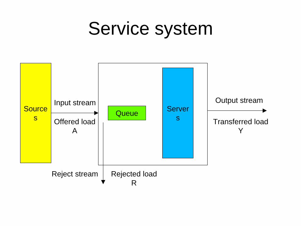
Service system

Source

s

Input stream

Queue Server

s

Output stream

Reject stream

Offered load

A

Transferred load

Y

Rejected load

R

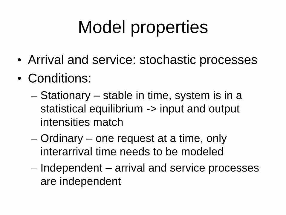
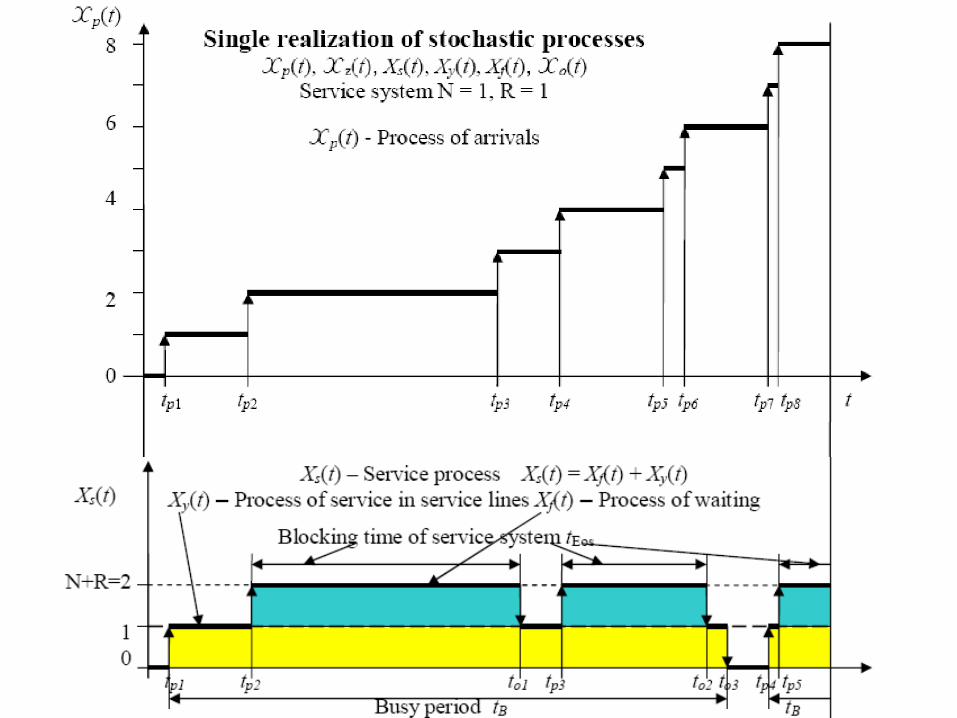
Model properties

• Arrival and service: stochastic processes

• Conditions:

– Stationary – stable in time, system is in a

statistical equilibrium -> input and output

intensities match

– Ordinary – one request at a time, only

interarrival time needs to be modeled

– Independent – arrival and service processes

are independent

Kendall’s classification

• Kendall introduced A/B/N(/M) notation

– A: statistical distribution of arrival process

– B: statistical distribution of service process

– N: number of service lines

– M: size of queue - not compulsory

• Where A and B may be:

– M: Markovian, Poisson process, exp. Dist

– D: Deterministic or Uniform

– G: General

– Ek: Erlang with parameter k

Poisson process

• Mostly M for Markovian is used.

• Assumes a Poisson process – Memoryless – arrival of one request is independent of

others. Modelled by exp dist. of interarrival times. • Then the input rate [req/s] will have Poisson dist.

• The load [busy time/hour] will have Erlang dist.

• If there the request are more grouped – i.e. the distribution has higher dispersion

– In simulation, use Pareto or Weibull dist.

• Then with the same average arrival rate, the average waiting time will be higher.

Exponential distribution

CDF: f(t;λ) = λ e- λ t PDF: F(t; λ) = 1 - e -λ t

Poisson distribution

System types

• Open system

– Number of customers not known

– Characterized by arrival rate

System types

• Closed system

– Fixed number of customers

– Alternating between two states

• Thinking, Requesting service

Operational Analysis

• Analyzing (part of) a queuing system as a "black box", with one input for jobs and one output for jobs

• The internal structure of the system (queuing network) is unknown

– The distribution of inter-arrival times is unknown

– The service times distribution is unknown

• Can be used to derive simple relationships, mostly between mean values of the system’s parameters (not distributions of e.g. que.lengths)

Utilization

• U = b / T – Utilization is the fraction of busy time to total

• Dimensionless [s/s]

• λ = X = a / T = d / T – Arrival rate=throughput is the number of

arriving=departing jobs per time [1/s]

• s = b / d – Service time is busy time per job [s]

• U = λs = Xs

• also s = 1 / μ -> U = λ / μ – If λ > μ – utilization/intensity > 1, system unstable

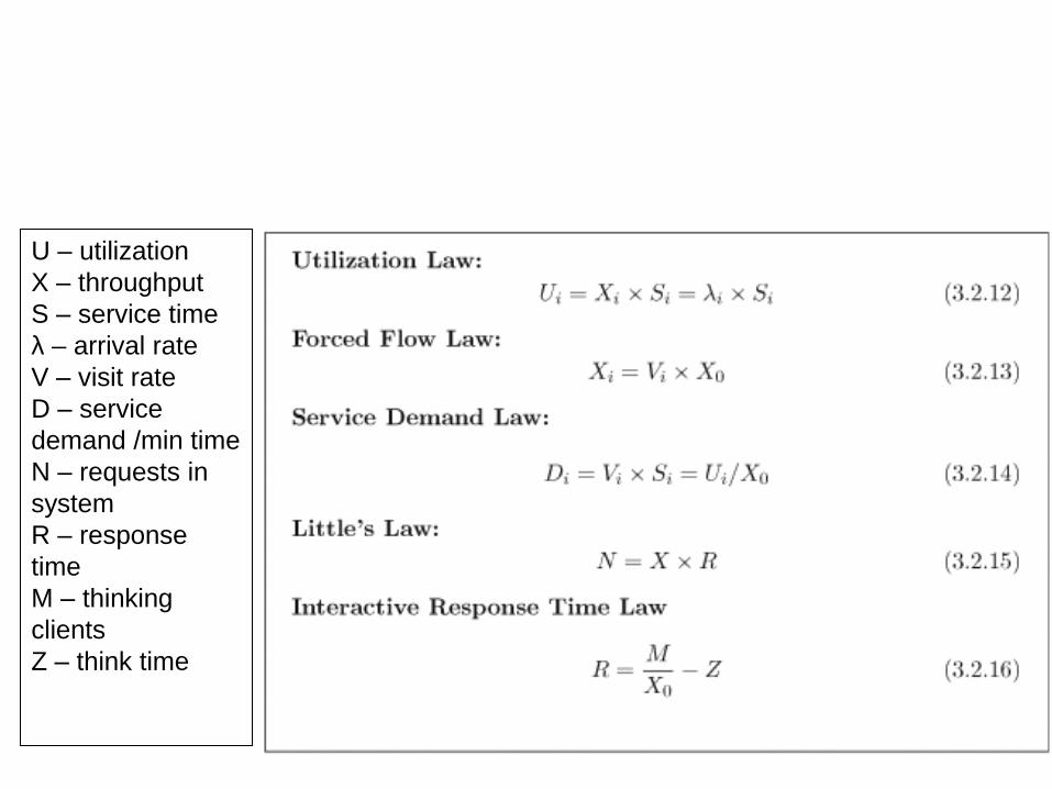
U – utilization

X – throughput

S – service time

λ – arrival rate

V – visit rate

D – service

demand /min time

N – requests in

system

R – response

time

M – thinking

clients

Z – think time

Little’s Law

Little’s Law

• Works with averages -> any steady-state

• On server only -> utilization law

• On server+queue -> computes queue length

Interactive Response Time Law

Latency vs. throughput (Z=0)

• In previous graph, vertical line – optimum

• To the left – light load – underutilized

– Throughput scales linearly by number of users, limited by sum of demands

– Latency constant

• To the right – heavy load – overutilized

– Throughput constant, limited by bottleneck resource

– Latency scales linearly

Asymptotics

Open system latency/throughput

M/M/1

• No longer operational analysis (G/G/*)

– We need the memoryless property of exp.dist.

– PASTA: Poisson Arrivals See Time Averages

• Distribution of the residual time until the next arrival is also exponentially distributed with the same parameter l as the time between consecutive arrivals.

• Distribution of the residual service time is the same as that of the service time.

• R = QS + S – avg. response time is avg. service time of jobs in the queue + the job being served

– Arriving job sees Q jobs ahead, no matter how much of the service time remains for the job(s) being served

M/M/1

• Using Little’s law on Q

– R = (λR)S + S

– > R = S / (1 - λS) • Using Little’s law on λS

– > R = S / (1 - U)

– Residence time depends on utilization.

• Stretch factor: (on basic service demand)

– F = R / S = 1 / (1 - S) = Q / mU

• Where Q is Unix load average, m number of CPUs, U percent CPU busy

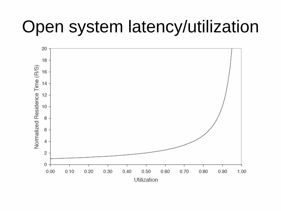
Open system latency/utilization

Multiserver latency/utilization

Markov chains

• Why does the queue behave like this?

– Birth-death Markov process

• States 0..J+1 (J - queue capacity)

– Last state blocking

– Arrival changes state to n+1, departure to n-1

– Probability of n jobs in the system pn=(1-U)Un

– Utilization U = 1 – p0

– Mean queue length E[n] = ΣnJnpn = U / (1-U)

PASTA and splitting

• The memoryless property allows splitting

and joining of request flows

– Each flow is a series of totally random events

– Splits defined by probabilities

• Jackson’s theorem translates to visit rates

– Allows construction of product-form queueing

networks

Queueing networks

• Basis of QN solving tools

•

• Qi(n) – average number in queue I with N

total jobs

• Nth job upon arrival sees the system with

N-1 jobs

– > Iterative algorithm

– Starts with Qi(0)=0, n=1 until n=N

Mean Value Analysis

Practical possibilities

• Profiling from server logs

– Also called Performance Monitoring

– Shows server load in the past (CPU, RAM,

network, number of processes, ..)

– Shows its periodicity, can do trend predictions

– Useful for existing applications to be migrated

to the cloud

– or as an estimate when done on a similar

application

A CPU utilization graph

Web server statistics

• Apache has mod_status

– Reports concurrency and throughput

– Combined with CPU utilization

• Allows to compute service demand, i.e. LATENCY

• And to estimate maximum throughput

– (service demand should be constant unless overloaded)

Tools

• Estimation of load profile from search

engine statistics

– Useful when marketing estimates the number

of users and you need to know when they'll be

accessing the site

– It will give you the time profile, but not the

actual amount of load

– Available from search engine term statistics or

some click counter providers

A graph from Google Insights

Load testing

• Good if you already have the application

– Or a prototype, or something similar to test

• Will give you the answer to:

– How much CPU/RAM does an app this complex written in this language need?

– How many requests per second does it give on this particular server?

• Will give you the possibility to optimize the server

• You'll need to know the app's usage scenarios

– To construct a good testing script/walk through the site

– To be able to translate numbers of users to requests/s

Load testing tools

• httperf – made by HP, quite old – Simulates an open system

• You give number of requests/s and a script

• Returns number of failures and timeouts – When low enough, the system can sustain the offered load

– Timeout needs to be set reasonably

» max 8s for whole page load is recommended

– Used by ramping up load until failure

• siege – Simulates a closed system

• You give number of users and think time (+ script)

• Returns measured response times – If below threshold (see above), system can sustain the load

Load testing tools

• JMeter – closed system (I think) – Strong side: proxy to capture scenarios – Weak side: written in Java :-E

• better than using scenarios is to test indiv. request types and construct a multiflow QN

• Tsung – my favorite

– closed system, but can be convinced to do open

– written in Erlang - very accurate

– also has a proxy

– automatic ramp-up scripts possible

– integrated graphical reporting with GnuPlot

Queueing network tools

• JMT (Java Modelling Tools) – Can do several models, graphical, parametric or script input – Logfile extraction, Markov Chain simulation, and Asymptotics – Best for quick analyses, manual usage

• PDQ (Pretty Damn Quick) – Core is in C

– Is a library with binding for several languages

– Only script input

– Best for integration in your programs

Conclusion – What to use

• Small company – Webhosting or VM rent

• Medium – Colocation + virtualization

• Medium with good conditions – Own

servers + virtualization

• Large – private or hybrid IaaS

• Web App. Startup – PaaS and have an

escape plan, or public IaaS

• Batch processing – public IaaS

Literature

http://www.elektrorevue.cz/clanky/02019/index.html

Daniel A. Menascé, Virgilio A.F. Almeida, Lawrence W. Dowdy: Performance by Design: Computer Capacity Planning by Example.

Neil J. Gunther: Analyzing Computer System Performance with Perl::PDQ Second Edition.

Tomáš Kalibera, Vlastimil Babka: Modeling in Performance Evaluation, lecture for Performance Evaluation, D3S MFF CUNI, 2013.

František Křížovský: Materiály k předmětu Teorie provozního zatížení, kat. telekomunikací FEL ČVUT, 2012.