Overhead Treatment

Overhead costs are significant for many manufacturing companies. Overhead costs are indirect manufacturing costs. Accountants use a cost allocation process to assign overhead costs to products. This chapter explores the underlying reasons for cost allocation, the use of predetermined overhead rates, the separation of mixed costs into their fixed and variable components, and capacity measures used to compute predetermined overhead rates. Regardless of the method the company uses to assign overhead to production, the company must dispose of the underapplied or overapplied overhead at the end of the year.

Overhead includes any indirect production cost incurred in manufacturing a product or providing a service. Indirect material and indirect labor are a part of overhead. Direct labor cost has been declining while overhead costs have been increasing. At many manufacturing companies, direct labor accounts for only 10 to 15 percent of the cost of production. This trend is due to the increased used of automation.

Overhead costs can be fixed or variable. Variable overhead costs include indirect material, lubricants, and the variable portion of electricity. Indirect labor paid on an hourly basis is a variable overhead cost. Depreciation using the units-of-production method or service-life method is another example of a variable overhead cost. Fixed overhead costs include straight-line depreciation on factory equipment, factory license fees, and factory insurance and property taxes. Indirect labor paid on a salary basis is a fixed overhead cost. The fixed portion of mixed overhead costs such as maintenance is also included in fixed overhead costs.

o Quality costs are an important category of overhead costs. Managers are concerned about quality at two levels. First, they are concerned about the customer’s perception of quality. Second, managers are concerned about the quality of the production process. Quality costs often amount to 20 to 25 percent of sales. Quality costs can be variable, step fixed, or fixed.

Two major categories of quality costs are (1) the cost of control and (2) the cost of failure to control. The cost to control includes prevention costs and appraisal costs. The cost of failure to control includes internal failure costs and external failure costs.

Prevention costs include employee training, improved production equipment, and researching customers’ needs.

Appraisal costs are the costs of inspection and monitoring.

Internal failure costs include the costs of scrap and rework.

1

External failure costs include handling customers’ returns due to poor quality, warranty costs, and handling customers’ complaints.

A company must accumulate overhead costs over a period and allocate the overhead costs to the products manufactured or services rendered during the period. Cost allocation is assigning indirect costs to one or more cost objects using some reasonable basis. Cost allocations are involved in a number of accounting procedures. In cost accounting, the accountant must allocate overhead costs to products using predictors or cost drivers. This process reflects the cost principle, which requires that all production costs attach to the products manufactured.

Three primary reasons for allocating overhead costs to products are as follows: (1) to calculate a full cost of the product, (2) to motivate the manager to manage costs efficiently, and (3) to analyze alternative courses of action for planning, controlling, and decision making. The first reason relates to financial accounting standards that require that full cost must include the indirect costs of production. Nonfactory overhead costs are not usually allocated to products under generally accepted accounting principles. The other two reasons for overhead allocation relate to internal purposes. A company may use different methods to allocate overhead for different purposes.

Companies can use either an actual cost system or a normal cost system to allocate overhead costs to production. In an actual cost system all production costs are actual costs.

o An actual cost system does not provide actual overhead costs until the end of the period. Managers need timely cost information to make good operating decisions. Therefore, many companies use a normal cost system.

o A normal cost system uses actual costs for direct material and direct labor and a predetermined overhead rate for overhead costs. The accountant computes the predetermined overhead rate by dividing the budgeted overhead costs for the period by the budgeted activity level for the same period. The period generally used to determine the overhead rate is one year. The overhead charged to work in process is the predetermined rate multiplied by the actual activity level. This is known as the applied overhead. Applied overhead thus is the amount of overhead assigned to Work in Process Inventory. Applied overhead is equal to the predetermined rate multiplied by the actual activity. The company could use separate accounts to record actual overhead and applied overhead or use a single account. Additionally, the company could use separate accounts for fixed and variable overhead or multiple overhead accounts by

2

activity or department. If the company uses separate accounts for fixed and variable overhead, the accountant must separate mixed costs.

Three reasons exist for using a predetermined overhead rate. First, a predetermined overhead rate allows the company to charge overhead costs to products during the period rather than at the end of the period. Second, predetermined overhead rates compensate for changes in actual overhead costs unrelated to the activity level. Third, predetermined overhead rates can overcome the problem of changes in the activity level that do not affect actual fixed overhead costs. Changes in the activity level do not affect fixed overhead costs, but changes in the activity level cause actual fixed overhead costs to vary on a per-unit basis. Using a predetermined overhead rate reduces such per-unit cost fluctuations.

The activity base the company uses to apply overhead cost should bear a logical relationship to the overhead cost incurred. Using production volume as the activity base makes sense if the company makes only one product. To allocate overhead cost to multiple products, the company must use an activity measure common to all the products. Preferably, the base should be a cost driver. Historically, many companies have used direct labor hours or direct labor cost to allocate overhead cost to production. Using direct labor hours or direct labor cost in highly-automated plants results in extremely high overhead rates and distorted product costs. The high overhead rate occurs because overhead costs are higher in automated plants while direct labor hours and direct labor cost are lower. Machine hours may be a more reliable base in automated plants. Also, some companies use activities such as machine setups, number of defects, and material handling time to assign certain overhead costs to products.

 

A company debits Manufacturing Overhead for actual overhead costs and credits various accounts as appropriate. A company applies overhead by debiting Work in Process Inventory and crediting Manufacturing Overhead. The Manufacturing Overhead account will have a balance at the end of the period. If actual overhead is greater than the applied overhead, then overhead is underapplied and the Manufacturing Overhead account will have a debit balance. If actual overhead is less than the applied overhead, then overhead is overapplied and the Manufacturing Overhead account will have a credit balance. A company must close the balance in the Manufacturing Overhead account. If the balance is not

3

material, the accountant closes it to Cost of Goods Sold. If the balance is material, the accountant must allocate it pro rata among Work in Process Inventory, Finished Goods Inventory, and Cost of Goods Sold.

o Two causes of underapplied and overapplied overhead are (1) a difference between actual and budgeted costs and (2) a difference between actual activity and activity or capacity used to compute the fixed overhead application rate.

 

To compute the per-unit fixed overhead costs, management must specify the capacity level used for the denominator. Capacity is a measure of production volume or some other activity base.

o Possible capacity measures are theoretical capacity, practical capacity, normal capacity, and expected capacity.

Theoretical capacity is the maximum potential activity for a particular period assuming that everything works perfectly.

Practical capacity is the production the company could achieve taking regular operating interruptions into consideration.

Normal capacity is the long-run average capacity considering cyclical fluctuations.

Expected capacity is the anticipated activity level for the upcoming period based on the current budget. Management often uses expected capacity in computing the predetermined overhead rate.

Appendix

Some companies use a single overhead rate for the entire plant, but a single rate is often not adequate for management’s needs. Departmental overhead rates usually provide better information to management because departments have different manufacturing processes and cost drivers. Some departments are more labor intensive than other departments, and some departments are more machine intensive than others.

Least squares regression analysis is a statistical method that analyzes the relationship between dependent and independent variables. Least squares regression analysis helps in developing an equation to predict an unknown value of a dependent variable from the known values of one or more independent variables. If multiple independent variables exist, least squares regression analysis can be used to determine the independent variable that is the best predictor of the dependent variable.

4

Simple regression analysis uses only one independent variable to predict the dependent variable. If more than one independent variable exists, the process is called multiple regression. Simple regression uses the linear formula y = a + bX. Least squares regression analysis determines the fixed costs (a) and the per-unit variable cost (b). The company then uses this formula to predict total mixed costs for any activity level within the relevant range.

Least squares regression analysis determines the line that best fits the data points. This line is called the regression line. The regression line minimizes the sum of the squares of the deviations between the data points and the line. Accountants can use least squares regression analysis to separate mixed costs into their fixed and variable components and predict total mixed costs at a different activity level within the relevant range.

Cost driverLet's start with an example. Suppose you and your friend established a company that produces valves used in automotive industry and named this company Friends Corporation. How much should you charge for one valve in order to stay in business? How many valves should be sold in a given month at a given price to cover your costs?

These questions can be answered with the aid of cost information. Cost information can support managers in decision-making. Let us define a cost.

Cost is a payment of cash or its equivalent for the purpose of generating revenues.

In case of the valve production business we have purchased materials cost, labor costs, depreciation costs, rent costs, insurance costs, etc. All these costs are incurred for the purpose of generating profit from the product sales.

In financial accounting, costs and expenses are used interchangably. In managerial accounting, costs differ from expenses. Cost is the amount of resources given up in order to receive some good or service and represents future economic benefit to a company. An asset is a cost. As future economic benefit of an asset decreases, the original cost of the asset expires and the cost becomes an expense. Expenses are matched with revenues on the income statement. A good example for understanding a cost and expense would be a fixed asset. When it is purchased, it is a cost to an entity and is shown on the balance sheet. When the fixed asset is used, it is depreciated and a portion of the cost becomes a depreciation expense, which is included in the income statement and matched with the revenue generated during the period.

Costs are determined by the manufacturing process and primarily depend on the volume of production. Some costs change in proportion to units produced, some only slighly react to changes in production, and others don't change at all. The factors impacting changes in costs are cost drivers defined as follows:

5

Cost driver is any activity that causes change of costs over a given period of time. These activities are also called activity bases or activity drivers.

In our example of valve production, we would like to know how much material to buy to ensure uninterrupted production process. Common sense suggests that amount of material we will need to purchase is driven by the number of valves we produce. Therefore, the production level is the cost driver for material costs. Other examples of costs and their cost drivers are maintenance expense and number of hours equipment is used, or hourly labor costs and how many hours employees work per day.

2. Cost behavior. Reaction of costs to changes in activityIn the previous section we discussed costs and cost drivers. We will continue by discussing in more detail how costs react to changes in activity.

For successful planning, managers must be able to predict how cost will behave under certain circumstances.

Cost behavior is the manner in which a cost changes in relation to changes in the related activity.

Understanding of how costs behave in a particular situation is crucial for decision-making process in an organization. Cost behavior information allows managers:

To prepare budgets To predict cash flows

To plan dividend payments

To establish selling prices

Depending on the cost behaviors, there are four common cost types, which are variable, fixed, mixed, and step-variable costs.

Methods for separating mixed costsManagement usually needs to know what fixed and variable costs are included into mixed costs. This is required for budgeting and planning purposes, among others. Using the total costs and the associated activity level, it is possible to break out the fixed and variable components. There are three methods for separating a mixed cost into its fixed and variable components:

High-low method Scatter-graph method

Method of least squares

6

High-low methodWhen using the high-low method, the highest point and the lowest point are used to create the cost formula. The high point is defined as the point with the highest activity and the low point is defined as the point with the lowest activity. Using the lowest and highest activity levels it is possible to estimate the variable cost per unit and the fixed cost component of mixed costs.

Illustration 14: Total costs of Friends Corporation over the last six months

Month Vales Production

Total Cost

July 10,000 $44,000August 15,000 $60,000September 23,000 $85,000October 21,000 $75,000November 19,000 $70,000December 28,000 $98,000

The lowest level of production was in July and the highest level of production was in December. The difference between the number of units produced and the difference between the total cost at the highest and lowest levels of production are shown below:

  Production Total CostHighest Level 28,000 units $98,000Lowest Level 10,000 units $44,000Difference 18,000 units $54,000

As the total fixed cost does not change with changes in volume of production, the difference in the total cost is the change in the total variable cost. So, if we divide the difference in total cost by difference in production, we will have an estimate of the variable cost per unit:

Variable Cost per Unit = $54,000 / 18,000 units = $3

The variable cost per unit is $3. The fixed cost will be the same at both the highest and the lowest levels of production because fixed costs stay constant. In order to estimate the fixed cost, we have to subtract the estimated total variable cost from the total cost:

Total Cost = Variable Cost per Unit x Units of Production + Fixed Cost

Highest level:

$98,000 = $3 x 28,000 + Fixed cost

7

Fixed cost = $14,000

Lowest level:

$44,000 = $3 x 10,000 + Fixed cost

Fixed cost = $14,000

The fixed cost is equal to $14,000. Now, knowing the fixed cost and variable cost per unit we can estimate total cost for the planned production level using the formula below:

T = F + V x N,

where T is Total Cost, F is Fixed Cost, V is Variable Cost per Unit and N is number of units to be produced.

The above methodology is the high-low method of separating mixed costs. The advantage of this method is its simplicity. However, this method ignores all data points other than the highest and the lowest activity levels. The highest and the lowest activity point often do not represent the rest of the points, which leads to possible inaccuracy of the final results. It is the main disadvantage of this method.

In order to get more precise results, it is better to use the scatter-graph method or the method of least squares.

Scatter-graph methodThe scatter graph method (also called scatter plot or scatter chart method) involves estimating the fixed and variable elements of a mixed cost visually on a graph.

The scatter-graph method requires that all recent, normal data observations be plotted on a cost (Y-axis) versus activity (X-axis) graph. Vertical axis of graph represents total costs and horizontal axis shows the volume of related activity.

Let us again use the example of Friends Corporation and review their activities for the last six months (see Illustration 14 from the previous section). First step is to plot the points, according to given data. Then a line that most closely represents a straight line composed of all the data points should be drawn. The graph using data points from Illustration 14 is shown on Illustration 15.

Illustration 15: Scatter graph

8

The point where this line intersects the vertical axis is the fixed costs, or $14,000 in our case. The angle (slope) of the line can be calculated to give a fairly accurate estimate of the variable cost per unit. We can see from the graph that production of 20,000 valves will cost Friends Corporation $75,000 and production of 25,000 valves will cost $90,000. Knowing this information we can calculate the variable cost per unit.

X2-X1 = 

$90,000 - $75,000 = 

$15,000 =  $3

Y2-Y1 25,000 - 20,000 5,000

When two variables are known, we may use them in the cost formula:

Y = F + V x X,

where F is fixed costs, V is variable cost per unit, and X is production level (may be different values).

So, the cost formula looks like this:

Y = $14,000 + $3 x X

Using this formula we can predict the total cost of activity in the range of 10,000 to 28,000 valves per month and then separate them into fixed and variable components. For example, assume that production of 24,000 valves is planned for the next period. Using the formula we can predict that total costs would be:

Y = $14,000 + $3 x 24,000 = $86,000

9

Of this total cost, $14,000 is fixed and $72,000 is variable, for a total of $86,000 ($14,000 + $72,000).

This method is simple to use and provides clear representation of correlation between costs and volume of activity. However, the disadvantage of this method is difficulties that may appear when determining the location of the best-fit line.

Method of least squaresThe most robust method of separating mixed costs is the least-squares regression method. This method requires the use of thirty or more past data observations for both the activity level (in units) and the total cost. The method of least squares identifies the line that best fits the data points (the sum of the squared deviations is minimized). This method is the most sophisticated and provides the user with a measure of the goodness of fit, which can be used to assess the usefulness of the cost formula. Usually this method requires the use of software packages, and therefore, will not be discussed in this lecture.

Fixed costsFixed costs remain constant within a relevant range of time or activity.

However, fixed costs per unit usually change with changes in the activity base. Insurance costs, rent costs, salaries of accounting personnel are typical fixed costs.

For example, Friends Corporation pays property insurance in amount of $50,000 per year. It is a fixed cost that does not vary with the number of produced valves; whether we produce 10,000 or 50,000 valves, our plant will still be assessed $50,000 in property insurance per year. Although the total fixed cost remains the same as the number of valves produced changes, the fixed cost per valve changes. The more valves are produced, the less the fixed cost per unit is. Illustration 5 shows this relationship.

Illustration 5: Fixed cost of property insurance at different production levels

Valves Produced

Property Insurance

Property Insurance per Valve

Calculation

10,000 $50,000 $5.00 $50,000 / 10,000 20,000 $50,000 $2.50 $50,000 / 20,000 30,000 $50,000 $1.67 $50,000 / 30,000 40,000 $50,000 $1.25 $50,000 / 40,000 50,000 $50,000 $1.00 $50,000 / 50,000

The data from the table above can also be presented in a graph. Illustration 6 demonstrates how the property insurance cost behaves when total production changes.

10

Illustration 6: Total fixed cost graph

Note that the property insurance cost line starts at $50,000 and does not change with the increase in the number of units produced. That is because fixed cost remains constant within a relevant range.

Illustration 7 shows how the fixed cost of property insurance behaves on per-unit basis as production changes.

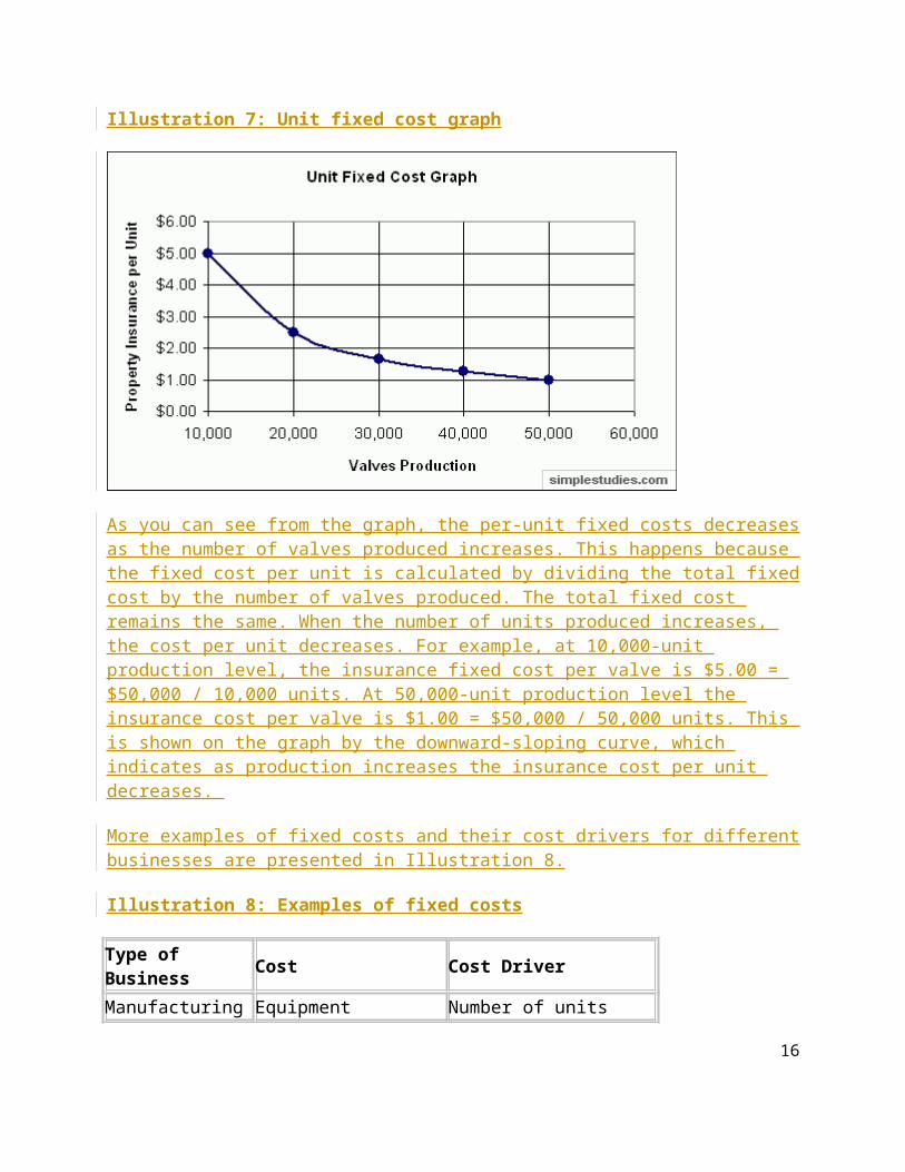
Illustration 7: Unit fixed cost graph

11

As you can see from the graph, the per-unit fixed costs decreases as the number of valves produced increases. This happens because the fixed cost per unit is calculated by dividing the total fixed cost by the number of valves produced. The total fixed cost remains the same. When the number of units produced increases, the cost per unit decreases. For example, at 10,000-unit production level, the insurance fixed cost per valve is $5.00 = $50,000 / 10,000 units. At 50,000-unit production level the insurance cost per valve is $1.00 = $50,000 / 50,000 units. This is shown on the graph by the downward-sloping curve, which indicates as production increases the insurance cost per unit decreases.

More examples of fixed costs and their cost drivers for different businesses are presented in Illustration 8.

Illustration 8: Examples of fixed costs

Type of Business Cost Cost DriverManufacturing Equipment depreciation Number of units producedRestaurant Rent cost Number of clients Taxi Insurance Number of miles drivenHotel Property tax Number of rooms occupiedPrint house Advertising costs Number of printed out pages Hospital Property Insurance Number of patients

Fixed costs can be classified as avoidable (discretionary) fixed costs and unavoidable (committed) fixed costs.

Avoidable (discretionary) fixed costs are costs that are not required to be incurred.

In other words, you will stay in business if you do not incur such costs. For instance, Friends Corporation may spend $5,000 per year on advertising. This is a fixed cost.  However, it is avoidable because the company can stop advertising and still stay in business (although sales volume may suffer).

Unavoidable (committed) fixed costs are costs you have to incur if you want to stay in business.

For example, the property tax, office rent, and depreciation expenses are unavoidable fixed costs. Friends Corporation will not be able to continue its business if the company does not pay property tax (authorities will take action to collect), does not have an office from which it runs the business, or does not buy equipment (and incurs depreciation expenses) to produce valves.

Step-variable costs

12

We have defined two basic types of costs which are variable costs and fixed costs. Another cost type is a step-variable cost which is defined as follows:

Step-variable costs are costs that stay fixed over a range of activity, and then change after this range is overcome. In other words, these costs change in increments.

Step-variable costs include characteristic of both variable and fixed costs in a way that (a) step-variable costs do change as production level changes, althrough (b) step-variable costs change only when a production level (range of activity) is overcome. Within that range of activity, step-variable costs remain fixed. The major differences between step-variable costs and fixed costs are that step-variable costs are changed by activity (rather than by a management decision) and step-variable costs are more easily changed compared to fixed costs.

To illustrate step-variable costs, let us return to our example with valve production. One employee can operate equipment to produce 100 valves per day. If 320 valves need to be produced, Friends Corporation would hire four employees (three employees won't be enough because three employees can only produce 300 valves). If the valves production requirement is increased to 400 units, four workers will still be able to cope with the load. However, for 410 valves, an additional, fifth employee would be needed. Thus, the payroll costs change in steps, from costs for four employees for 320 units and 400 units, to payroll costs for five employees for 410 units.

Illustration 9: Step-variable cost graph

Illustration 9 describes a step-variable payroll cost, where the width of each step represents the volume of activity (valves production) needed before the step-variable cost increases to the next level (an additional employee is hired). Once the next level is achieved, the payroll costs increase

13

and remain constant until the next level is achieved again. Narrow width means that cost is sensitive to fairly small fluctuations in related activity.

Other examples of step-variable costs and their cost drivers are provided in the Illustration 10.

Illustration 10: Examples of step-variable costs

Type of Business Cost Cost DriverManufacturing Number of workers Number of units producedRestaurant Number of waiters Number of clients Hotel Number of housekeepers Number of rooms occupiedHospital Number of nurses Number of patients

Mixed costsMixed costs contain components of both variable and fixed cost behavior patterns. Mixed costs are sometimes called semivariable or semifixed costs.

The fixed component of a mixed cost is a minimum cost of supplying a resource, and the variable component is the costs that fluctuate depending on changes of activity levels.

Suppose Friends Corporation uses rented machinery. The rental charges are $1,000 per year, plus $1 for each machine hour used. If the machinery is used for 1,000 hours, then the total rental charge is $2,000 ($1,000 + 1,000 hrs x $1). The table below shows the relationship between the variable and fixed costs, total cost and machine hours.

Illustration 11: Mixed cost table

Number of Machine Hours

Variable Cost per Hour

Variable Cost

Fixed Cost

Total Costs

Total Costs Calculation

500 $1.00 $500 $1,000 $1,500 $500 + $1,0001,000 $1.00 $1,000 $1,000 $2,000 $1,000 + $1,0001,500 $1.00 $1,500 $1,000 $2,500 $1,500 + $1,0002,000 $1.00 $2,000 $1,000 $3,000 $2,000 + $1,0002,500 $1.00 $2,500 $1,000 $3,500 $2,500 + $1,0003,000 $1.00 $3,000 $1,000 $4,000 $3,000 + $1,000

The following formula is used in the table:

Mixed Cost = Fixed Cost + Variable Cost

14

Illustration 12 graphically demonstrates this relationship. You can see that the mixed cost line starts at the fixed-cost point of the vertical axis ($1,000 in our case) and then increases to the right. The minimal value of the mixed cost is equal to its fixed part and is applicable when machinery is not used at all; therefore, only fixed portion of the cost is incurred and equals $1,000. When machinery is used, the variable cost ($1 per hour) is added to the fixed cost to arrive at total (mixed) cost.

Illustration 12: Mixed costs graph

More examples of mixed costs and their cost drivers are provided in the Illustration 13.

Illustration 13: Examples of mixed costs

Type of Business Cost Cost DriverManufacturing Equipment rental Number of machine hoursConsulting Company Consultant's wage Number of clients Hotel Maid wages Number of rooms cleanedPrint house Photocopier rental Number of pages printed out

Relevant rangeWe have mentioned a relevant range before when we talked about step-variable costs:

Relevant range is the volume of activity, over which cost behavior stays valid.

15

Friends Corporation can produce from 10,000 to 50,000 valves per year. So, the relevant range for Friends Corporation is the range of normal activity from 10,000 to 50,000. Within this relevant range all fixed costs, such as rent, equipment depreciation, and administrative salaries remain constant. If Friends Corporation decides to produce more valves, they have to hire additional staff and rent more equipment, which will result in an increase of fixed costs. On the contrary, if production level is reduced, Friends Corporation has to reduce staff and rental expenses, so fixed costs will decrease.

Methods for separating mixed costsManagement usually needs to know what fixed and variable costs are included into mixed costs. This is required for budgeting and planning purposes, among others. Using the total costs and the associated activity level, it is possible to break out the fixed and variable components. There are three methods for separating a mixed cost into its fixed and variable components:

High-low method Scatter-graph method

Method of least squares

High-low methodWhen using the high-low method, the highest point and the lowest point are used to create the cost formula. The high point is defined as the point with the highest activity and the low point is defined as the point with the lowest activity. Using the lowest and highest activity levels it is possible to estimate the variable cost per unit and the fixed cost component of mixed costs.

Let us assume that Friends Corporation incurred the following costs during the last six months:

Illustration 14: Total costs of Friends Corporation over the last six months

Month Vales Production

Total Cost

July 10,000 $44,000August 15,000 $60,000September 23,000 $85,000October 21,000 $75,000November 19,000 $70,000December 28,000 $98,000

The lowest level of production was in July and the highest level of production was in December. The difference between the number of units produced and the difference between the total cost at the highest and lowest levels of production are shown below:

16

  Production Total CostHighest Level 28,000 units $98,000Lowest Level 10,000 units $44,000Difference 18,000 units $54,000

As the total fixed cost does not change with changes in volume of production, the difference in the total cost is the change in the total variable cost. So, if we divide the difference in total cost by difference in production, we will have an estimate of the variable cost per unit:

Variable Cost per Unit = $54,000 / 18,000 units = $3

The variable cost per unit is $3. The fixed cost will be the same at both the highest and the lowest levels of production because fixed costs stay constant. In order to estimate the fixed cost, we have to subtract the estimated total variable cost from the total cost:

Total Cost = Variable Cost per Unit x Units of Production + Fixed Cost

Highest level:

$98,000 = $3 x 28,000 + Fixed cost

Fixed cost = $14,000

Lowest level:

$44,000 = $3 x 10,000 + Fixed cost

Fixed cost = $14,000

The fixed cost is equal to $14,000. Now, knowing the fixed cost and variable cost per unit we can estimate total cost for the planned production level using the formula below:

T = F + V x N,

where T is Total Cost, F is Fixed Cost, V is Variable Cost per Unit and N is number of units to be produced.

The above methodology is the high-low method of separating mixed costs. The advantage of this method is its simplicity. However, this method ignores all data points other than the highest and the lowest activity levels. The highest and the lowest activity point often do not represent the rest of the points, which leads to possible inaccuracy of the final results. It is the main disadvantage of this method.

17

In order to get more precise results, it is better to use the scatter-graph method or the method of least squares.

Statistics Tutorial: A Simple Regression ExampleIn this lesson, we apply regression analysis to some fictitious data, and we show how to interpret the results of our analysis.Note: Regression computations are usually handled by a software package or a graphing calculator. For this example, however, we will do the computations "manually", since the gory details have educational value.

Problem StatementLast year, five randomly selected students took a math aptitude test before they began their statistics course. The Statistics Department has three questions.

What linear regression equation best predicts statistics performance, based on math aptitude scores?

If a student made an 80 on the aptitude test, what grade would we expect her to make in statistics?

How well does the regression equation fit the data?

How to Find the Regression EquationIn the table below, the xi column shows scores on the aptitude test. Similarly, the yi column shows statistics grades. The last two rows show sums and mean scores that we will use to conduct the regression analysis.

Student xi yi (xi - x) (yi - y) (xi - x)2 (yi - y)2 (xi - x)(yi - y)

1 95 85 17 8 289 64 136

2 85 95 7 18 49 324 126

3 80 70 2 -7 4 49 -14

4 70 65 -8 -12 64 144 96

5 60 70 -18 -7 324 49 126

Sum 390 385 730 630 470

Mean 78 77

The regression equation is a linear equation of the form: ŷ = b0 + b1x . To conduct a regression analysis, we need to solve for b0 and b1. Computations are shown below.

18

b1 = Σ [ (xi - x)(yi - y) ] / Σ [ (xi - x)2] b1 = 470/730 = 0.644

b0 = y - b1 * x

b0 = 77 - (0.644)(78) = 26.768

Therefore, the regression equation is: ŷ = 26.768 + 0.644x .

How to Use the Regression EquationOnce you have the regression equation, using it is a snap. Choose a value for the independent variable (x), perform the computation, and you have an estimated value (ŷ) for the dependent variable.

In our example, the independent variable is the student's score on the aptitude test. The dependent variable is the student's statistics grade. If a student made an 80 on the aptitude test, the estimated statistics grade would be:

ŷ = 26.768 + 0.644x = 26.768 + 0.644 * 80 = 26.768 + 51.52 = 78.288

Warning: When you use a regression equation, do not use values for the independent variable that are outside the range of values used to create the equation. That is called extrapolation, and it can produce unreasonable estimates.

In this example, the aptitude test scores used to create the regression equation ranged from 60 to 95. Therefore, only use values inside that range to estimate statistics grades. Using values outside that range (less than 60 or greater than 95) is problematic.

How to Find the Coefficient of DeterminationWhenever you use a regression equation, you should ask how well the equation fits the data. One way to assess fit is to check the coefficient of determination, which can be computed from the following formula.

R2 = { ( 1 / N ) * Σ [ (xi - x) * (yi - y) ] / (σx * σy ) }2

where N is the number of observations used to fit the model, Σ is the summation symbol, xi is the x value for observation i, x is the mean x value, yi is the y value for observation i, y is the mean y value, σx is the standard deviation of x, and σy is the standard deviation of y. Computations for the sample problem of this lesson are shown below.

σx = sqrt [ Σ ( xi - x )2 / N ] σx = sqrt( 730/5 ) = sqrt(146) = 12.083

σy = sqrt [ Σ ( yi - y )2 / N ] σy = sqrt( 630/5 ) = sqrt(126) = 11.225

19

R2 = { ( 1 / N ) * Σ [ (xi - x) * (yi - y) ] / (σx * σy ) }2 R2 = [ ( 1/5 ) * 470 / ( 12.083 * 11.225 ) ]2 = ( 94 / 135.632 )2 = ( 0.693 )2 = 0.48

A coefficient of determination equal to 0.48 indicates that about 48% of the variation in statistics grades (the dependent variable) can be explained by the relationship to math aptitude scores (the independent variable). This would be considered a good fit to the data, in the sense that it would substantially improve an educator's ability to predict student performance in statistics class.

Correlation coefficientFrom Wikipedia, the free encyclopedia

Jump to: navigation, search

Correlation Coefficient may refer to:

Pearson product-moment correlation coefficient , also known as r, R, or Pearson's r, a measure of the strength of the linear relationship between two variables that is defined in terms of the (sample) covariance of the variables divided by their (sample) standard deviations

Correlation and dependence , a broad class of statistical relationships between two or more random variables or observed data values

Goodness of fit , which refers to any of several measures that measure how well a statistical model fits observations by summarizing the discrepancy between observed values and the values expected under the model in question

Coefficient of determination , a measure of the proportion of variability in a data set that is accounted for by a statistical model; often called R2; equal in linear regression to the square of Pearson's product-moment correlation coefficient

Intraclass correlation , a descriptive statistic that can be used when quantitative measurements are made on units that are organized into groups; describes how strongly units in the same group resemble each other.

Rank correlation , the study of relationships between different rankings on the same set of items

o Spearman's rank correlation coefficient , which measures how well the relationship between two variables can be described by a monotonic function

o Kendall tau rank correlation coefficient , which measures the portion of ranks that match between two data sets.

In statistics, the Pearson product-moment correlation coefficient (sometimes referred to as the PMCC, and typically denoted by r) is a measure of the correlation (linear dependence) between two variables X and Y, giving a value between +1 and −1 inclusive. It is widely used in the sciences as a measure of the strength of linear dependence between two variables. It was developed by Karl Pearson from a similar

20

but slightly different idea introduced by Francis Galton in the 1880s.[1][2] The correlation coefficient is sometimes called "Pearson's r."

Interpretation of the size of a correlation

Several authors have offered guidelines for the interpretation of a correlation coefficient. Cohen (1988), has observed, however, that all such criteria are in some ways arbitrary and should not be observed too strictly. The interpretation of a correlation coefficient depends on the context and purposes. A correlation of 0.9 may be very low if one is verifying a physical law using high-quality instruments, but may be regarded as very high in the social sciences where there may be a greater contribution from complicating factors.

21

Correlation Negative Positive

None −0.09 to 0.0 0.0 to 0.09

Small −0.3 to −0.1 0.1 to 0.3

Medium −0.5 to −0.3 0.3 to 0.5

Large −1.0 to −0.5 0.5 to 1.0