mohdruhaizie.commohdruhaizie.com/hs223/hs223finalyear/fyp/fypsitimasha… · web viewthe main...

CHAPTER ONE

INTRODUCTION

1.1 Introduction

Among several type of pollution, the most observed and largely distributed pollution

is air pollution, either ambient air pollution (which always related to the industry,

vehicle and agricultural activities) or indoor air quality (related to the household

properties and air change). Natural sources of pollution such as emission from

volcanoes may hugely pollute the air we breathe but in instance. However,

anthropogenic sources, although pollute the atmosphere in small portion compared

to natural sources done, but when it is done for every seconds, the impact may be

larger. Annually, it is estimated from human activities itself there are two billion metric

tonnes of pollution released to the earth’s sky, which is in the end this pollution is

trapped up there, thus overwarm the earth surface back then. There are traces of

human-made contaminants found everywhere in the globe, including remnants of the

two billion metric tons of pollutions emitted into the atmosphere by human activities

annually (Cunningham et-al, 2012).

Air pollution has been an issue which arise not only among modern economic

countries such as United States and countries in the European block, but also to the

developed countries and the third world countries. Even the developed countries,

which most of the economic sources are depend on manufacturing industry and

agriculture are more concern about air pollution matter recently and they’re struggle

to overcome this issue. In some cases this requires lifestyle changes or different

ways of doing things to bring about progress, but as the Chinese Philosopher Lao

Tsu wrote, “A journey of a thousand miles must begin with a single step”.

As mentioned before, the source of air pollution can be either natural or man-made.

Both can be divided specifically into two which is stationary or mobile sources. One

of the most significant mobile sources of air pollution in many urban areas worldwide,

including in Malaysia is due to vehicular emission.

1

Nitrogen oxides (NOX), sulphur dioxides (SO2), and carbon monoxides (CO) are

some examples of pollutant properties in the emission. Carbon monoxides are

caused by the incomplete burning process in the vehicle engine and both nitrogen

oxides and sulphur dioxides occurred from the evaporation of the fuel. Other than

these three, particulate matter (PM) and ozone (O3) are also culprits from motor

vehicle emission.

There are many factors that contribute to the concentration and relative mixture of

the pollutants. It was depends on vehicle speed, acceleration, deceleration, the

amount of time vehicles spend idling, stopping and waiting, especially at major

junction in urban area. The pollutants also related to vehicle type (e.g., light or heavy-

duty vehicles) and age, operating and maintenance condition, exhaust treatment,

type and quality of fuel, wear of part and engine lubricant used.

1.2 Problem Statement

The main sources of air pollution in Malaysia are emissions from stationary sources,

motor vehicles and open burning. According to the Compendium of Environment

Statistics 2012, motor vehicles contributed 68.5% of the emission to the atmosphere.

Stationary sources and other sources accounted for 26.4% and 5.1% respectively.

There are increases in emission of all type of pollutant from motor vehicle between

2011 and 2012. Emission of carbon monoxide increased by 6.5% followed by sulphur

dioxide (5.1%) and 4.5% increment for each nitrogen dioxide and particulate matter.

In 1997, there were roughly 8.5 million registered motor vehicles in Malaysia,

climbing at the rate of more than 10% every year. According to 1997 figures, the

estimated quantities of air pollutants released by these vehicles were 1.9 million tons

of carbon dioxide, 224,000 tons of nitrogen oxide, 101,000 tons of hydrocarbons,

36,000 tons of sulphur dioxide and 16,000 tons of particulate matter. Mean values for

the years 1993 to 1997 show that the amount of air pollutants from mobile emission

sources accounts for about 81% of all air pollution occurring in Malaysia. The

problem will clearly become even more critical as the number of motor vehicles

keeps on increasing.

This situation is afraid can influence the human health condition especially those who

work or live near traffic environment such as traffic police, toll gate staff, road

2

construction worker as well as enforcement officer from Custom, Immigration &

Quarantine at ground crossing check-point, either between Malaysia-Thailand in

Bukit Kayu Hitam (Kedah), Padang Besar (Perlis), Pengkalan Hulu (Perak), Rantau

Panjang and Pengkalan Kubor (Kelantan) or Malaysia-Singapore (Johor Causeway

in Johor Bahru and Secondlink Causeway in Gelang Patah) in Peninsular Malaysia.

Motor vehicle emissions can cause numerous health problems and aggravate

chronic respiratory conditions (e.g. asthma, lung disease, cancer). Carbon monoxide

emissions can cause dizziness, confusion, headaches and in high concentrations

lead to death. Nitrogen oxide can restrict the respiratory system in humans, and can

contribute to the formation of acid rain when combined with water vapour in the air.

Volatile organic compounds can react with nitrogen oxides and sunlight and forming

ozone, which can also cause respiratory conditions in people (e.g. coughing, chest

tightness). Particulate matter, either inhalable particles, fine particles or ultrafine

particles which emitted from vehicles can be inhaled into the lungs, which can have

negative health impacts. Air toxicants (e.g. benzene, poly-aromatic hydrocarbon)

include substances that can cause cancer and organ damage in humans, and have

toxic impacts on natural environments. (California Air Resources Board, 2005).

1.3 Study justification

Indoor Air Quality Assessment in Entry Point Terminal is one of the indicators set by

World Health Organization to recognize Designated Point of Entry, which fulfil the

requirements in Annex 1B of International Health Regulations 2005. Sultan Abu

Bakar (CIQ) Complex located at Tanjung Kupang, Johor is one of the Designated

Point of Entry recognized by WHO, but without completely fulfil the requirement of

indoor air quality.

Therefore, studying a part of emission that may threat indoor air quality in this Entry

Point not only beneficial to gain baseline data, but also to trigger awareness among

Enforcement Officer regarding hazardous substances which they may inhale or

indoor air condition they faced while on duty.

This study is done to identify whether the indoor air quality in the immigration station

is in the hazardous level or not. This study also aims to identify the location that

mostly problem with the indoor air pollution.

3

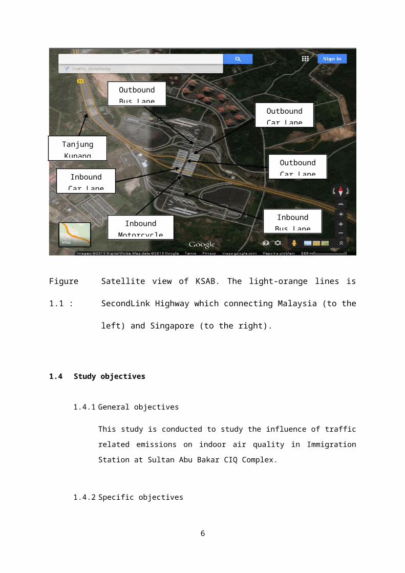
Figure 1.1 : Satellite view of KSAB. The light-orange lines is SecondLink Highway

which connecting Malaysia (to the left) and Singapore (to the right).

1.4 Study objectives

1.4.1 General objectives

This study is conducted to study the influence of traffic related emissions on

indoor air quality in Immigration Station at Sultan Abu Bakar CIQ Complex.

1.4.2 Specific objectives

1.4.2.1 To identify the level of pollutant (carbon monoxide (CO), carbon

dioxide (CO2), particulate matter (PM10) and relative humidity

(%RH)) at the Immigration Station.

4

Outbound Car Lane

Outbound Car Lane

Outbound Bus Lane

Tanjung Kupang

Inbound Car Lane

Inbound Motorcycle Lane

Inbound Bus Lane

1.4.2.2 To compare pollutant concentration at the Immigration Station with

Industry Code of Practice on Indoor Air Quality (ICOP IAQ) 2010.

1.4.2.3 To determine the correlation between pollutant, number of vehicle

and day.

1.5 Study hypothesis

1.5.1 There are non-compliances of several parameters with the ICOP IAQ 2010.

1.5.2 There are strong correlations between pollutant and number of vehicle and

day.

1.6 Conceptual framework

Figure 1.2 : Conceptual Framework of the study

5

AIR POLLUTION

NATURAL ANTROPHOGENIC

STATIONARY MOBILE SOURCE

VEHICLE EMISSION

VOC RESPIRABLE PARTICULATE

PM10

COMBUSTION PRODUCT

SULFUR DIOXIDE

NITROGEN OXIDE

CARBON DIOXIDE

CARBON MONOXIDE

1.6.1 Conceptual definitions

a) Air Pollution

The introduction of particulates, biological molecules, or other harmful materials

into the atmosphere which they can be a source of adverse effect on human,

animal, plant, built environment and the entire ecosystem (World Health

Organization).

Meanwhile, the air pollutants are substances, either in form of solid particles,

liquid droplets or gases, both sourced from either anthropogenic activities or

natural fates. Both of the sources could be in form of stationary or in form of

mobile (U.S. Environmental Protection Agency)

b) Mobile source

Both natural and anthropogenic pollution source could be mobile source of

pollution. The example of natural mobile pollution source is sand storm which

bursting coarse particles into the air, while there are too many man-made

mobile pollution source, one of the major is from vehicle. Source of vehicular

pollutions are (1) coming from inside the engine caused by the combustion

processes, released through the exhaust pipeline; (2) coming from the wear of

tyre (friction between tyre and road surface); (3) substances that the vehicle

bring on it body/surface unintentionally such as dust; and (4) friction between

paint molecules and air velocity (U.S. Environmental Protection Agency)

c) Adverse impact

In year 2000, 6% of the annual total deaths among Austria, Switzerland and

France residents were due to air pollution, where half of it is sourced from

vehicle and traffic related air pollution. Bronchitis and asthma are among major

initial sickness that lastly results the damage of respiratory organs, followed by

death (Kunzli et al 2000).

6

1.6.2 Operational Definitions

a) Immigration Station

This study will be covering Immigration Station inside Sultan Abu Bakar CIQ

Complex compound, which located at

i. Motorcycle lane either inbounds to Malaysia from Singapore or outbound

to Singapore from Malaysia (the station is one-man booth which using

split unit air conditioning system, one unit per booth). Motorcyclist just

need to passed their passport through the opening of a small sliding

window while they’re on their bike for travel clearance etc. For each

bound, the number of motorcycle lane booth is 10. During very heavy

peak hour, a car lane may be converted it function as motorcycle lane as

well;

ii. Car lane (which included van, multipurpose vehicle (MPV), sport utilities

vehicle (SUV) and four wheels drive (4WD) etc.) either inbound to

Malaysia from Singapore or outbound to Singapore from Malaysia (the

station is one-man booth which using split unit air conditioning system,

one unit per booth). Driver and passengers just need to pass their

passports through the opening of a small sliding window while they’re in

the vehicle for travel clearance; and

iii. Bus lane (in this study, only one bus lane is selected which is the one

inbounds to Malaysia from Singapore). It is located in a building such as

in other public transport terminal, where there are 12 immigration

counters, 4 of it is for Malaysian Passport Holder, other for International

Passport Holder. There are queue hall where travellers, coming out from

the bus along with their carriage, walking to the queue hall and waiting

their turn to pass their passport to the on duty Immigration Officer for

travel clearance. The hall use centralized outdoor coil cooling air

conditioning system.

7

b) In-situ Measurement

This study is conducted by measuring a real-time 30-minutes averaged data

using suitable measurement and monitoring device. The data may be logged

into data logging memory of the device, but for the safety of the data

collected, the data is manually copied into a written form. The detail regarding

measurement techniques and methodologies is discussed in Chapter 3:

Methodology.

c) Day

Based on the information from Immigration Department regarding the volume

and trend of movement crossing the terminal:

i. Weekday or working day is based on Singapore’s weekday or working

day (from Monday to Friday). Weekday for Johor residents is from

Sunday until Thursday (since January 1, 2014).

ii. Weekend or non-working day is also based on Singapore’s weekend or

non-working day (public holiday) which is from Saturday to Sunday.

Weekend for Johor residents is from Sunday until Thursday (since

January 1, 2014).

d) Peak hours

Peak hours are defined as period in a day where the volume of vehicles or

travellers is higher compared to the other period within a day. In Sultan Abu

Bakar CIQ Complex, the weekday peak hours are when vehicles or travellers

(by all modes of vehicle: motorcycle, car or bus) crossing outbound from

Malaysia to Singapore (mostly due to the working purpose) which is usually

starting from 4.00 am until 10.00 am, and when they’re crossing inbound from

Singapore to Malaysia which is usually starting from 4.00 pm until 10.00 pm.

8

CHAPTER TWO

LITERATURE REVIEW

2.1 Introduction

The following literature review is an analysis on the existing body of knowledge in

these areas of work, based on legal requirements, journals, articles, agency reports

and others information sources.

2.1.1 Source of pollution

Air pollution is contamination of the indoor or outdoor environment by any chemical,

physical or biological agent that modifies the natural characteristics of the

atmosphere. Household combustion devices, motor vehicles, industrial facilities and

forest fire are common sources of air pollution.

Air pollution happens due to the presence of anthropogenic pollutants and non-point

source pollutants in the air. Non-point source pollutants come from sources that

cannot be accurately identified. These pollutants have diffusively and indirectly

contributed towards the degradation of environment. According to Callan and

Thomas (2004), several researches have validated the identified determinants of the

world’s air pollution. For example, in the investigation done by Zhu (2012), it is found

that the vehicle emissions and industrial waste from nearby Pearl River Delta

degrade the quality of the air in Hong Kong. Marco (2011) posits that air pollution is

majorly caused by combustion engine vehicles such as cars, trucks and planes. Air

pollution from cars and trucks is split into primary and secondary pollution, which is

the primary pollution is emitted directly into the atmosphere and secondary pollution

results from chemical reactions between pollutants in the atmosphere.

9

2.1.2 Parameter contributed

i. Temperature and Relative Humidity ASHREA 55(2004), defines thermal comfort as “that condition of mind

which expresses satisfaction with the thermal comfort environment”.

The perception of thermal comfort is affected by body temperature

that is interactively influenced by personal activity, clothing, and the

environmental factors of air temperature, air movement, and RH.

ASHRAE 55(2004), standard for relative humidity of 30-60% and

Temperature of 20-26°C. According to ASHRAE 62 (2007) humidity is

not a major concern in ventilation system design. Humidity has only a

small effect on thermal sensation and perceived air quality in the

rooms of sedentary occupancy, however, long-term high-humidity

indoors may cause microbial growth, and very low humidity (15-20 per

cent) with increase temperature may cause dryness and irritation of

eyes and airways (Cheong et al, 2005).

ii. Carbon Dioxide (CO2)

A study carried out by Mui et al, (2005) shown a correlation

determining the average concentration in the occupied period for a

ventilated space could be significantly increased with increasing

number of sampling points in the space. The results shown of the

spatial mean indoor CO2 concentration in the office, it was found that

when the number of sampling points required for IAQ measurement

was reduced by 50%, the probability of obtaining the sample-spatial

average concentration at the same confidence level would be

decreased by 10%. It can be conclude that the selection of the

sampling location in a space allows relatively expedient evaluations of

IAQ.

iii. Carbon Monoxide (CO)

A survey on the status of indoor air pollution in residential buildings

using different fuels in China (Z.Wang et al, 2004) indicate that the

concentrations of four indoor pollutants resulting from gas combustion

were less than those resulting from coal combustion. This can be

conclude as combustion issue in the indoor environment is not

10

significant in this office area as the sources only comes from the

ambient air environment supply to the AHU system.

iv. Total Volatile Organic Compound (TVOC)

Sources of VOC in the building could be from the painting, furniture,

glue or air refresher. Indoor pollution caused by VOCs is an important

aspect of IAQ which raises particular concern since many organic

indoor pollutants are either known, or are suspected to be allergic,

carcinogenic, neurotoxin, immunotoxic, irritant or indicative of SBS. It

may derive from the human activities and interior building materials in

tight building design. Study found that off-gassing chemicals would

adsorb onto another building material and re-emit at a later time (AIHA

1993). Study by Lundgren (1994) show the chemical pollutant

emissions may affect the indoor environment in several ways: affect

health and well-beings, give rise to troublesome odors, contaminate

other materials, result in discoloration of adjacent materials, and

condense on electronic equipment and result in mal-operation.

v. Particulate Matter (PM)

PM is a combination of fine solids and aerosols that are suspended in

the air. Particles come from different sources. PM can be solid, like

dust, ash or soot. PM can also be liquid, aerosols or solids suspended

in liquid mixtures. There are different sizes of particles. The ones of

most concern are small enough to lodge deep in the lungs where they

can do serious damage. They are measured in microns. The largest of

concern are 10 microns in diameter (PM10). The group of most

concern is 2.5 microns in diameter or smaller (PM2.5). Some of these

are small enough to pass from the lung into the bloodstream, just like

oxygen molecules. High levels of particle pollution have been found to

cause or are likely to cause many serious health effects, including:

death from respiratory and cardiovascular causes, higher risk of heart

attacks and strokes, increased hospital admissions and emergency

room visits for cardiovascular and respiratory diseases, and increased

severity of asthma attacks in children. Breathing high levels over a

long time may decrease the development of the function of the lungs

as children grow and may cause lung cancer.

11

2.2 Legal requirements

There are several Malaysian standards regarding the IAQ start from the legislative

requirement of Occupational Safety & Health Act 1994 (OSHA 1994) to Industry

Code Of Practice On Indoor Air Quality 2010 (ICOP-IAQ 2010). The parameters

including six chemicals which are Carbon Dioxide (CO2), Carbon Monoxide (CO),

Total Volatile Organic Compounds (TVOC), Formaldehyde, Respirable Particulates

(PM10) and Ozone and three physicals which are Temperature, Humidity (RH) and

Air Movements.

2.3 Regulations / Guidelines / Methods

i. Industry Code of Practice on Indoor Air Quality 2010.

2.4 Journals / articles

2.4.1 Air pollution from motor vehicles

Atmospheric pollutants are responsible for both acute and chronic effects on

human health (WHO, 2000). Motor vehicle emission has been recognized as

one of the major source of air pollution, particularly in highly urbanized areas.

Based on 1992 study by the Japan International Cooperation Agency (1993),

it was concluded that the air pollution problem in Kuala Lumpur is relatively

serious when compares with accepted air quality standards. The annual and

daily readings for CO, Ozone and PM10 have exceeded the standard.

Unfortunately follow-up studies in 1994 continued to shows serious problem

and motor vehicles again found to be the main source of air pollution (Walsh

et al, 1997).

Studies around the world have indicated that CO is the most abundant

pollutant per annum with practically 70% of all CO gas produces solely by

motor transport vehicles (Kiely, 1997). According to Davis and Cornwell in

1998, CO is a colourless, odourless, tasteless and non-irritating gas but can

12

be lethal to human beings within minutes at high concentrations exceeding

12,800 parts per million (ppm).

In urban environments and especially in those areas where population and

traffic density are relatively high, human exposure to hazardous substances is

expected to be significantly increased. This is often the case near busy traffic

points in city center where urban situation may contribute to the creation of

poor air dispersion conditions giving rise to contamination hotspots (Sotiris et

al, 2003).

2.4.2 Vehicle related air pollutants

Engine exhaust, from diesel, gasoline, and other combustion engines, is a

complex mixture of particles and gases, with collective and individual

toxicological characteristics. Vehicle tailpipe emissions includes criteria air

pollutants such as particulate matter and carbon monoxide, ozone precursor

compounds such as nitrogen oxides (NOx) and other hazardous air pollutants

(e.g., air toxics) not regulated by EPA as criteria pollutants.

Particulate matter represents a heterogeneous group of physical entities.

Based on toxicological and epidemiological research, smaller particles and

those associated with traffic appear more closely related to health effects. PM

characteristics that may contribute to toxicity include metal content, presence

of polycyclic aromatic hydrocarbons and other toxic organic components.

Other particulate matter characteristics that may be important to human health

effects include mass concentration, number concentration, acidity, particle

surface chemistry, metals, carbon composition and origin. Collectively

exposure fine particles are strongly associated with mortality, respiratory

diseases and lung development in children, and other endpoints such as

hospitalization for cardiopulmonary disease.

Motor vehicles also emit air toxics. EPA has identified six priority mobile

source air toxics, including benzene, 1,3-butadiene, formaldehyde,

acetaldehyde, acrolein, naphthalene and diesel exhaust. Similarly, the

California Air Resources Board (CARB) has identified 10 air toxics of concern,

five of which are emitted by on-road mobile sources: benzene, 1,3-butadiene,

13

formaldehyde, acetaldehyde, and diesel PM (California Air Resources Board,

2001).

Mobile source air toxics are known or suspected to cause cancer or other

serious health or environmental effects. Benzene is of particular concern

because it is a known carcinogen and most of the nation’s benzene emissions

come from mobile sources. Diesel exhaust particulate matter (DPM) is a toxic

air contaminant and known lung carcinogen resulting from combustion of

diesel fuel in heavy duty trucks and heavy equipment. People who live or work

near major roads or spend a large amount of time in vehicles are likely to

have higher exposures and higher risks.

2.4.3 Roadway air pollutants in infiltration into indoor environments

Research shows consistent strong correlations between outdoor and indoor

concentrations of traffic related air pollutants including constituents of

particulate matter such as benzene and PAHs, and Volatile Organic

Compounds. In one study, exposure in indoor environments to particulates,

measured via light absorption was 19-26% higher even when accounting for

indoor sources such as appliances for cooking and heating.

2.4.4 Health and traffic-related pollution

There is a higher prevalence of respiratory symptoms among children living

near motorways or freeways, and also a higher prevalence of chronic

coughing, wheezing, asthma attacks and rhinitis in areas with higher truck

traffic density (Oosterlee et al 1996; van Vliet et al 1997; van Der See et al

1999; Venn et al 2001; Lin et al 2002). Other studies have also found a strong

association between decreased lung function of children living near

motorways and increased air pollution levels from truck and motor vehicle

traffic (Brunekreef et al 1997; Nakai et al 1999).

A cross-sectional survey of children's health was undertaken in New South

Wales between October and December 1993 to investigate the relationship

between outdoor air pollution and the respiratory health of children aged 8–10

years (Lewis et al 1998). This cross-sectional study of primary school children

showed an important association between relatively low levels of particulate

14

air pollution and respiratory symptoms. This is consistent with similar cross-

sectional studies from other countries.

Prasanthi and Rajeswari (2003) conducted a survey at major traffic points in

Kurnool town to investigate the effect of vehicular emissions on the health of

53 traffic policemen. It was found that these personnel were directly exposed

to vehicular emissions for nearly 8 hours per day. The main symptoms

observed were cough 80%, breathlessness 20%, headache and dizziness

30% and passage of black sputum in the morning 3%and also conducted

pulmonary function test (PFT) on these personnel. Some of them exhibited

normal pulmonary function test. About 60% showed mild to moderate

obstruction, out of which 65% were non-smokers and 35% were smokers. In

case of 20% of smokers the obstruction was severe .It was concluded that

traffic policemen were suffering from respiratory disorders due to exposure to

vehicular pollution.

Results from clinical, epidemiological and animal studies are converging to

indicate that short-term and long-term exposures to traffic-related pollution

especially particulates have adverse cardiovascular effects. Short-term

exposure to fine particulate pollution exacerbates existing pulmonary and

cardiovascular disease and long-term repeated exposures increases the risk

of cardiovascular disease and death.

Traffic density in school districts in Munich was associated with decreases in

forced vital capacity (FVC), forced expiratory volume in 1 second (FEV1),

FEV1/FVC and other measures although the 2-kilometer (km) areas the use

of sitting position for spirometry and problems with translation for non-German

children were limitations. Brunekreef et al used distance from major roadways

considered wind direction and measured black smoke and NO2 inside

schools. They found the largest decrements in lung function in girls living

within 300m of the roadways.

15

CHAPTER THREE

METHODOLOGY

3.1 Study Location

Sultan Abu Bakar CIQ Complex is located in Bukit Kucing, Mukim Tanjung Kupang,

at the western region of Johor Bahru District, which is about 15 kilometres from

Gelang Patah Town; 25 kilometres from Johor State New Administrative Centre

(JSNAC) in Kota Iskandar, Nusajaya; 40 kilometres from the centre of Johor Bahru

metropolitan; and 50 kilometres from the Senai Airport. The GPS coordinate is

1.378066, 103.599218.

This complex can be accessed via the inner route of Jalan Tanjung Kupang – Gelang

Patah or via SecondLink Highway (E3). However, as this complex is restricted area,

the entrance connected with the inner route can only be accessed by authorised

personnel.

Historically, this complex and SecondLink Highway were developed in 1990s to ease

the traffic problems between Malaysia and Singapore at Tanjung Puteri CIQ Complex

(Johor Causeway). It’s a new link between Malaysia (at Kampung Tanjung Kupang)

and Singapore (at Tuas).

As the climate in Malaysia is wet and dry throughout all over the year, the same goes

here. However, as this location is out the hilly area of Peninsular Malaysia, it’s open

to both Western and Eastern Monsoon. As December is a season peak for Eastern

Monsoon, raining and storm will be more frequent here.

16

3.2 Study Design

This is a cross-sectional study in which the data is collected from several samples at

one point in time and then by comparing the difference between characteristic found

in all samples, a conclusion is made of (Leslie G.P. and Mary P.W., 2009).

3.3 Study Variables

3.3.1 Independent Variable

a) Location of sampling either at the Motorcycle lane, Car lane or Bus lane

b) Number of vehicle passed the sampling location

c) Time of sampling either morning, noon, afternoon, evening or night

d) Days either it is on Singapore’s weekdays (working days) and weekends

(non-working days).

3.3.2 Dependent Variable

a) In-situ parameters of indoor air quality including temperature, relative

humidity percentage, carbon monoxide concentration, carbon dioxide

concentration, ozone concentration, total volatile organic compound

concentration and particulate matter concentration.

3.3.3 Confounding Variable

a) Ambient air quality parameters, which may penetrate/flow into the

sampling location.

b) Pressure status of the sampling location either positive pressure or

negative pressure. Positive pressure area will let the air from inside flow-

out thus contaminant properties maybe push out to the outside of the

area. Negative pressure area will let the air from outside flow-in thus

contaminant properties maybe pull in from the outside of the area.

17

c) Number of vehicle at the other nearby lane may also effect the

measurement.

3.4 Sampling and data collection

3.4.1 Sampling locations are selected randomly from a total of 20 booths in

Motorcycle lane (inbound and outbound) (6 booths selected, three for each

bound), 44 booths in Car lane (inbound and outbound) (6 booths selected,

three for each bound) and 4 halls in Bus lane (inbound and outbound) (only

one hall is selected, for the inbound). All measurement devices are placed at

the centre in each location during sampling activity, which may not disturbed

the activities of the Immigration Officer on duty as well as the traveller

movement. This is also a measure to protect the safety of the instrument.

3.4.2 All probes are set to be at the same height as breathing area in sitting position

(approximately 1 metre height from the floor level).

3.4.3 Each sampling is done for average 30-minutes at each sampling location

where the duration of sampling is set for 30-minutes, with data is logged for

every 2 minutes and time constant is 3 seconds, except for pbbRAE 3000.

3.4.4 Prior to each sampling, all devices will be set to zero calibration using Zero

Filter, except for pbbRAE 3000.

3.4.5 The data log is downloaded into the computer for analysis.

3.4.6 The analysis is done using SPSS Version 16.0

3.5 Instrumentation

3.5.1 TSI® DustTrakTM II Model 8530 with Zero Filter

3.5.2 TSI® QTrakTM Model 7575-X with Indoor Air Quality Probe

3.5.3 Tripod or Moveable Cabinet

18

3.5.4 TSI® TrakProTM Software

3.5.6 Microsoft Excel 2010

3.5.7 IBM SPSS 16.0

3.5.8 Equipment & What-to-do Checklist

3.5.9 Simple Interview Question Checklist

3.5.10 Camera

3.6 Data Analysis

3.6.1 Graph manipulation – Microsoft Excel 2010

3.6.2 Statistical analysis – IBM SPSS 16.0

3.7 Study Limitation

3.7.1 Time limitation for to get the equipment, study execution (short time

permission given), analysis and report writing

3.7.2 Monitoring equipment limitation: only managed to get a set of instrument,

does limit the simultaneously reading.

19

CHAPTER FOUR

RESULT

4.1 Specific objective (1) :To identify the level of pollutants (CO2, CO, PM10 & %RH) at Immigration Station

The measurement activities has been done from 03/12/2014 until 07/12/2014, where

on 03/12/2014 and 07/12/2014 measurement is done in Immigration Station (Cars &

Motorcycles – Both Outbound to Singapore and Inbound to Malaysia) while on

04/12/2014 and 06/12/2014 measurement is done in Immigration Station (Bus –

Inbound to Malaysia).

The measurement is done to monitor the concentration of carbon dioxide (CO2),

carbon monoxide (CO), particulate matter (PM10), and relative humidity (%RH).

In total, there are 37 measurements have been done during this study (N=37).

Among this, the total number of measurement on Immigration Station at the lane of

Motorcycle bound to Singapore (Motor-Out) and at the lane of Motorcycle bound to

Malaysia (Motor-In) are 11 (N=11) while the total number of measurement on

Immigration Station at the lane of Car bound to Singapore (Car-Out) and at the lane

of Car bound to Malaysia (Car-In) is 10 (N=10). The number of measurement done in

Immigration Station at the Bus lane bound to Malaysia is 16 (N=16) and no

measurement done in Bus lane bound to Singapore.

Immigration Station Motorcycle Lane

Car Lane Bus Lane

Day

Weekday (Working Day) 6 6 8

Weekend (Non-Working Day) 5 4 8

Total 11 10 16

Table 4.1 : Number of measurement done by day and immigration station

20

motor-o

ut

motor-o

ut

motor-o

ut

motor-i

n

motor-i

n

motor-i

nbus-i

nbus-i

nbus-i

nbus-i

nbus-i

nbus-i

nbus-i

nbus-i

n

motor-i

n

motor-i

n

motor-o

ut

car-o

ut

1033

218

623

138

133

7155

415

094

016

752

499

16 7 10 5 9 8 15 12 13 10 12 12 20 6 12 8 41 67 36 59 67 47 8733

Figure 4.1 : Number of motorcycle (motor), car and bus passing the Immigration Station

which were assigned as sampling point during study measurement

Figure 4-1 above shows the number of motorcycle (motor), car and bus which

passing the Immigration Station which were been assigned as sampling point lane

during measurement done. The background panel colour is to differentiate the day

when was the measurement been conducted. The yellow panel indicate that the

measurements were done at 30-minutes averaged at each lane on weekdays or

working days (which were on December 3, 2014 for each motorcycle lane and car

lane; and on December 4, 2014 for the bus lane). The white background panel

indicate that the measurements were done at 30-minutes averaged at each lane on

weekends or non-working days (which were on December 6, 2014 for bus lane and

on December 4, 2014 for each motorcycle lane and car lane).

Result for measurement done in the Immigration Station at Motorcycle Lane (both

bounds)

a) Number of motorcycles crossed the check point during weekday and weekend

Figure 4-1 above shown that the number of motorcycle passed the Immigration

Station at the motorcycle lane (outbound to Singapore and inbound to

Singapore) are 3,807 (95.56%) on the weekday (working day) and 177 (4.44%)

on weekend (non-working day). This difference is influenced by the number of

Malaysian who works in Singapore on every weekday, or Singaporean who lives

21

in Malaysia but riding back to Singapore for works on every weekday, whose

preferred travelling across both countries is easier by riding motorcycles. As

observed, most of the motorcycles crossing this entry point terminal on weekend

are purposely due to leisure and vacation (source: Immigration Department).

From the Table 4-2 in the next page, it is found that the mean for number of

motorcycle crossing the Immigration Station during study period is 634.5 (SD

323.251) with median is 588.50 (IQR 537) and skewness of the distribution curve

is -.322 (negative distribution, skewed to the left) for weekday and 66.0 (SD

13.675) with median is 67.00 (IQR 22.0) and skewness of the distribution curve

is .786 (positive distribution, skewed to the right) for weekend.

The ratio of the mean number of motorcycle crossing the Immigration Station in

weekday and weekend is 9.61. The number of motorcycle across this entry point

terminal is almost 10 times greater during weekday compared to the weekend.

Total mean for the number of motorcycle crossing the check-point (N=11) is

376.09 (SD 374.785) where the median is 133.00 and skewness is .749.

Figure 4.2 : The histogram and distribution curve regarding the descriptive statistic for

number of motorcycle cross the Immigration Station during weekdays and

weekends

22

Based on the figure above, it’s found that the frequencies of motorcycle number

which crossing the terminal during weekday and weekend is not normally

distributed, where the distribution curve is positively skewed.

Descriptives

Day Statistic Std. Error

No. of Motorcycle passed

the Imig. Station

Weekday Mean 634.50 131.967

95% Confidence Interval

for Mean

Lower Bound 295.27

Upper Bound 973.73

5% Trimmed Mean 640.22

Median 588.50

Variance 1.045E5

Std. Deviation 323.251

Minimum 133

Maximum 1033

Range 900

Interquartile Range 537

Skewness -.322 .845

Weekend Mean 66.00 6.116


for Mean

Lower Bound 49.02

Upper Bound 82.98


Median 67.00

Variance 187.000


Minimum 50

Maximum 87

Range 37


Skewness .786 .913

Table 4.2 : SPSS output for descriptive statistic regarding number of motorcycle cross

the Immigration Station during weekdays and weekends

23

b) Carbon monoxide (CO) concentration measurement

0

5

10

1520

25

30

35

4045

38.3

3.7 0.700000000000001

5.59.4

14

1.3 0.8 1.9 3.5

11.1

CO (motorcycle lane)

CO WEEK-DAYS

CO WEEK-ENDS

Time

conc

entr

ation

(ppm

)

Figure 4-3 (a) : CO concentration accumulated in the Immigration Station at motorcycle

lane during weekdays and weekends

Based on the Figure 4-3(a) above, it is shown that in most of the measurement

for CO which is done in Immigration Station at motorcycle lane were not

exceeding the acceptable limit of CO (ceiling limit of 10 ppm, indicated by

straight red line) on both weekday and weekend, except in two points for

weekday (each at CO concentration of 38.3 ppm and 14.0 ppm, respectively)

and another one point in the weekday which is the CO concentration nearly

exceed the limit (CO concentration 9.4 ppm), while for weekend, the only reading

over the acceptable limit is 11.1 ppm.

Based on the Table 4-3 below, for all CO concentration measured in motorcycle

lane, the mean of CO concentration is 8.2 ppm (SD 10.94 ppm) and median 3.7

ppm.

Based on Figure 4-3(b) below, from all 11 sampling done (N=11), it’s found that

the frequencies of CO concentration which is accumulated in the Immigration

Station at motorcycle lane is not normally distributed, where the distribution

curve is positively skewed.

24

Statistics

Carbon Monoxide

N Valid 11

Missing 0

Mean 8.200

Std. Error of Mean 3.2994

Median 3.700

Mode .7a


Variance 119.744

Skewness 2.413

Std. Error of Skewness .661

Range 37.6

Minimum .7

Maximum 38.3

Percentiles 25 1.300

50 3.700

75 11.100

a. Multiple modes exist. The smallest value is shown

Table 4.3 and Figure 4.3 (b) :

25

SPSS output for descriptive statistic regarding level of CO concentration during

measurement done in the Immigration Station at the motorcycle lane for both outbound and

inbound during weekday and weekend

c) Carbon dioxide (CO2) concentration measurement

0

200

400

600

800

1000

1200

619

466 471

834

537549

488

459

651594

477

CO2 (motorcycle lane)

CO2 WEEKDAYS

CO2 WEEKENDS

Time

Conc

entr

ation

(ppm

)

Figure 4.4 (a) : CO2 concentration which is accumulated in the Immigration Station at

motorcycle lane during weekdays and weekends

Based on the Figure 4-4(a) above, it is shown that all of the CO2 concentration

measured in Immigration Station at motorcycle lane were below the acceptable

limit of CO2 (ceiling limit of C1000 ppm, indicated by straight red line) on both

days. The highest recorded concentration of CO2 is 834 ppm during weekday

and 651 ppm during weekend.

As shown in Table 4-4 and Figure 4-4 (b) in the next page, for all CO2

measurement in motorcycle lane, the mean of CO2 concentration is 558.64 ppm

(SD 112.984 ppm) and median 537 ppm.

From all 11 sampling done (N=11), it’s found that the frequencies of CO2

concentration accumulated in the Immigration Station at motorcycle lane is not

normally distributed, where the distribution curve is positively skewed.

26

Statistics

Carbon Dioxide

N Valid 11

Missing 0

Mean 558.64


Median 537.00

Mode 459a


Variance 1.277E4

Skewness 1.573


Range 375

Minimum 459

Maximum 834


50 537.00

75 619.00


Table 4.4 and Figure 4.4 (b):

27

SPSS output for descriptive statistic regarding level of CO2 concentration during



d) Particulate matter (PM10) concentration measurement

0

0.02

0.04

0.06

0.08

0.1

0.12

0.14

0.16

0.086

0.044

0.033

0.0240.036

0.057

0.028 0.0320.035

0.0250.04900000000000

01

PM10 (motorcycle lane)

WEEKDAYS

WEEKENDS

Time

Conc

entr

ation

(mg/

kg)

Figure 4.5 (a) : PM10 concentration which is accumulated in the Immigration Station at

motorcycle lane during weekdays and weekends

Based on the Figure 4-5(a) above, it is shown that all of the PM10 concentration

measured in Immigration Station at motorcycle lane were below the acceptable

limit of PM10 (ceiling limit of 0.15 mg/m3, indicated by straight red line) on both

days. The highest recorded concentration of PM10 is 0.086 mg/kg during

weekday and 0.049 mg/kg during weekend. The conversion formula between

mg/m3 and mg/kg is that 1 mg/kg is equal to 1 mg/m3.

As shown in Table 4-5 and Figure 4-5 (b) in the next page, for all PM10

measurement in motorcycle lane, the mean of PM10 concentration is 0.0482

mg/kg (SD 0.018093 mg/kg) and median 0.03500.

28

From all 11 sampling done (N=11), it’s found that the frequencies of PM10

concentration accumulated in the Immigration Station at motorcycle lane is not

normally distributed, where the distribution curve is positively skewed.

Statistics

Particulate Matter

N Valid 11

Missing 0

Mean .04082

Std. Error of Mean .005455

Median .03500

Mode .024a

Std. Deviation .018093

Variance .000

Skewness 1.749


Range .062

Minimum .024

Maximum .086

Percentiles 25 .02800

50 .03500

75 .04900


29

Table 4.5 and Figure 4.5 (b):

SPSS output for descriptive statistic regarding level of PM10 concentration during



e) Relative humidity (%RH) measurement

0

10

20

30

40

50

60

70

80

90

100

76.8 74.469.7

61.967.9 69.8

60.5 60.653.3

71.1

92.6

%RH (motorcycle lane)

%RH WEEKDAYS

%RH WEEKENDS

Time

%

Figure 4-6 (a) : Relative humidity percentage which is accumulated in the Immigration

Station at motorcycle lane during weekdays and weekends

Based on the Figure 4-6(a) above, it is shown that all of the %RH measured in

Immigration Station at motorcycle lane were below the acceptable range of

(ceiling limit of 70% and floor limit at 40%, indicated by straight red line) on both

days. None of the reading found to be below than the lower limit of the range,

however several measurement found that it’s exceed or nearly exceed the upper

limit of the range. The highest recorded concentration of %RH is 76.8% during

weekday and 92.6% during weekend.

As shown in Table 4-6 and Figure 4-6 (b) in the next page, for all %RH

measurement in motorcycle lane, the mean of %RH is 68.964% (SD 10.4566%)

and median 69.700%.

30

From all 11 sampling done (N=11), it’s found that the frequencies of %RH

concentration accumulated in the Immigration Station at motorcycle lane is near

to the normal distribution. However the distribution curve is positively skewed.

Statistics

% Relative Humidity

N Valid 11

Missing 0

Mean 68.964


Median 69.700

Mode 53.3a


Variance 109.341

Skewness .905


Range 39.3

Minimum 53.3

Maximum 92.6


50 69.700

75 74.400


31


SPSS output for descriptive statistic regarding level of relative humidity percentage during



Result for measurement done in the Immigration Station at Car Lane (both bounds)

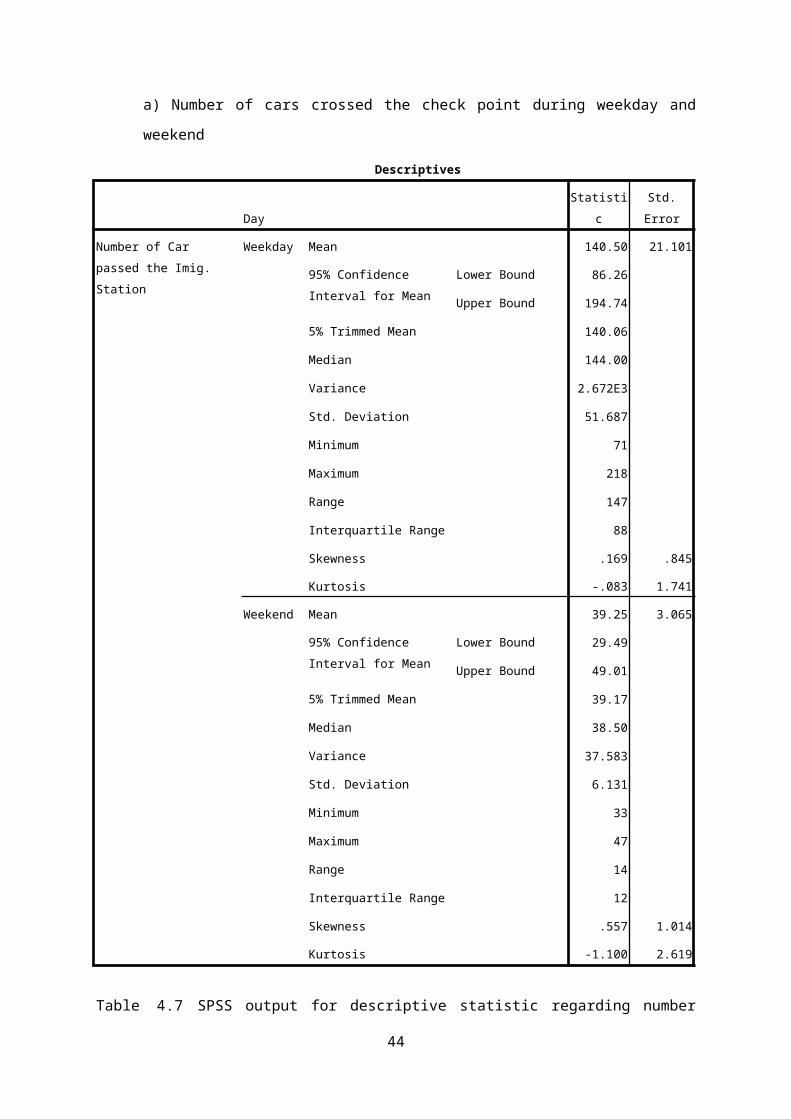
a) Number of cars crossed the check point during weekday and weekend

Descriptives


Number of Car passed the

Imig. Station



for Mean

Lower Bound 86.26

Upper Bound 194.74


Median 144.00

Variance 2.672E3


Minimum 71

Maximum 218

Range 147


Skewness .169 .845

Kurtosis -.083 1.741

32



for Mean

Lower Bound 29.49

Upper Bound 49.01


Median 38.50

Variance 37.583


Minimum 33

Maximum 47

Range 14


Skewness .557 1.014

Kurtosis -1.100 2.619

Table 4.7 : SPSS output for descriptive statistic regarding number of car across the

Immigration Station during weekdays and weekends

Figure 4-1 above shown that the number of car passed the Immigration Station

at the motorcycle lane (outbound to Singapore and inbound to Singapore) are

834 (76.32%) on the weekday (working day) and 260 (23.77%) on weekend

(non-working day). As in the motorcycle lane, this difference is influenced by the

number of Malaysian who works in Singapore, or Singaporean who lives in

Malaysia but driving back to Singapore for works.

From the Table 4-7 in the previous page, it is found that the mean for number of

car crossing the Immigration Station during study period is 140.50 (SD 51.687)

with median is 144.00 (IQR 88) and skewness of the distribution curve is .169

(positive distribution, skewed to the right) for weekday and 39.25 (SD 6.131) with

median is 38.50 (IQR 12) and skewness of the distribution curve is .557 (positive

distribution, skewed to the right) for weekend.

The ratio of the mean number of car crossing the Immigration Station in weekday

and weekend is 3.58. The number of car across this entry point terminal is

almost 3.6 times greater during weekday compared to the weekend.

33

Total mean for the number of car crossing the check-point (N=10) is 100.00 (SD

65.042) where the median is 85.00 and skewness is .597.

Figure 4.7 The histogram and distribution curve regarding the descriptive statistic for

number of car crossing the Immigration Station during weekdays and

weekends

Based on the figure above, it’s found that the frequencies of car number which

across the terminal during weekday and weekend is near to the normal

distribution, however the distribution curve is positively skewed.


0

5

10

15

20

25

30

3.2

0.1 0.11.2

3 2.40.1

0.700000000000001 1.6

25.3

CO (car lane)

CO WEEK-DAYS

CO WEEK-ENDS

Time

Conc

entr

ation

(ppm

)

34

Figure 4.8 (a) : CO concentration which is accumulated in the Immigration Station at the

car lane during weekdays and weekends

Based on the Figure 4-8(a) above, it is shown that in most of the measurement

for CO done in Immigration Station at car lane were not exceeding the

acceptable limit of CO (ceiling limit of 10 ppm, indicated by straight red line) on

both days except in one point at the weekend where the concentration of CO is

25.3 ppm.

Based on the Table 4-8 below, for all CO measurement in car lane, the mean of

CO concentration is 8.77 ppm (SD 7.6557 ppm) and median 1.4 ppm.


the frequencies of CO concentration accumulated in the Immigration Station at

car lane is not normally distributed, where the distribution curve is positively

skewed.

Statistics

Carbon Monoxide

N Valid 10

Missing 27

Mean 3.770

Median 1.400

Mode .1


Variance 58.609

Skewness 3.025


Range 25.2

Minimum .1

Maximum 25.3

Percentiles 25 .100

50 1.400

75 3.050

35

Table 4.8 and Figure 4.8(b)


measurement done in the Immigration Station at the car lane for both outbound and inbound

during weekday and weekend


0100

200300400

500600700

800900

1000

652

481403

572613

528558466

696

591

CO2 (car lane)

CO2 WEEKDAYS

CO2 WEEKENDS

Time

Conc

entr

ation

(ppm

)

Figure 4.9 (a) : CO2 concentration which is accumulated in the Immigration Station at car

lane during weekdays and weekends

36


measured in Immigration Station at car lane were below the acceptable limit of

CO2 (ceiling limit of C1000 ppm, indicated by straight red line) on both days. The

highest recorded concentration of CO2 is 652 ppm during weekday and 696 ppm

during weekend.


measurement in car lane, the mean of CO2 concentration is 558.64 ppm (SD

112.984 ppm) and median 537 ppm.


concentration accumulated in the Immigration Station at car lane is not normally


Statistics

Carbon Dioxide

N Valid 10

Missing 27

Mean 556.00

Median 565.00

Mode 403a


Variance 7.941E3

Skewness -.175


Range 293

Minimum 403

Maximum 696


50 565.00

37

75 622.75


Table 4.9 and Figure 4.9(b)


measurement done in the Immigration Station at the car lane for both outbound and inbound



0.000

0.020

0.040

0.060

0.080

0.100

0.120

0.140

0.160

0.0400.030 0.033

0.0260.040 0.0410.041 0.038

0.023 0.043

PM10 (car lane)

PM10 WEEKDAYS

PM10 WEEKENDS

Time

Conc

entr

ation

(mg/

kg)

38


car lane during weekdays and weekends


measured in Immigration Station at car lane were below the acceptable limit of

PM10 (ceiling limit of 0.15 mg/m3, indicated by straight red line) on both days. The

highest recorded concentration of PM10 is 0.043 mg/kg during weekend and

0.041 mg/kg during weekday. The conversion formula between mg/m3 and

mg/kg is that 1 mg/kg is equal to 1 mg/m3.


measurement in car lane, the mean of PM10 concentration is 0.03550 mg/kg (SD

0.007044 mg/kg) and median 0.03900.


concentration accumulated in the Immigration Station at car lane is not normally


Statistics

Particulate Matter

N Valid 10

Missing 27

Mean .03550

Median .03900

Mode .040a


Variance .000

Skewness -.811


Range .020

Minimum .023

Maximum .043


50 .03900

39

75 .04100




measurement done the Immigration Station at the car lane for both outbound and inbound



0

20

40

60

80

100

120

77.4 75.3 75.365.1

69

69.961.0 64.3

69.2

99.0

%RH (car lane)

%RH WEEKDAYS

%RH WEEKENDS

Time

%

40

Figure 4.11 (a) : Relative humidity percentage which is accumulated in the Immigration

Station at car lane during weekdays and weekends

Based on the Figure 4-11(a) above, it is shown that most of the relative humidity

measured in Immigration Station at car lane is above or nearly the acceptable

range of (ceiling limit of 70% and floor limit at 40%, indicated by straight red line)

on both days. None of the reading found to be below than the lower limit of the

range, however several measurement found that it’s exceed or nearly exceed the

upper limit of the range. The highest recorded concentration of %RH is 75.3%

during weekday and 99.0% during weekend.


measurement in car lane, the mean of %RH is 72.550% (SD 10.6774%) and

median 69.550%.


concentration accumulated in the Immigration Station at car lane is near to the

normal distribution. However the distribution curve is positively skewed.

Statistics

% Relative Humidity

N Valid 10

Missing 27

Mean 72.550

Median 69.550

Mode 75.3


Variance 114.007

Skewness 1.830


Range 38.0

Minimum 61.0

Maximum 99.0


50 69.550

41

75 75.825



measurement which is done in the Immigration Station at the car lane for both outbound and


Result for measurement done in the Immigration Station at Bus Lane

a) Number of bus crossed the check point during weekday and weekend

Descriptives


Number of Bus passed the

Imig. Station



for Mean

Lower Bound 7.04

Upper Bound 13.46


Median 9.50

Variance 14.786


Minimum 5

Maximum 16

Range 11

42


Skewness .369 .752



for Mean

Lower Bound 8.17

Upper Bound 15.08


Median 12.00

Variance 17.125


Minimum 6

Maximum 20

Range 14


Skewness .968 .752

Table 4.12 : SPSS output for descriptive statistic regarding number of bus across the

Immigration Station during weekdays and weekends

Figure 4-1 above shown that the number of bus passed the Immigration Station

at the bus lane (outbound to Singapore and inbound to Singapore) are 82

(46.86%) on the weekday (working day) and 93 (53.14%) on weekend (non-

working day). As in the bus lane, this difference is influenced by the number of

Malaysian who works in Singapore, or Singaporean who lives in Malaysia but

driving back to Singapore for works.

From the Table 4-12 in the previous page, it is found that the mean for number of

bus crossing the Immigration Station during study period is 10.25 (SD 3.845)

with median is 9.50 (IQR 7) and skewness of the distribution curve is .369

(positive distribution, skewed to the right) for weekday and 11.62 (SD 4.138) with

median is 12.00 (IQR 4) and skewness of the distribution curve is .968 (positive

distribution, skewed to the right) for weekend.

The ratio of the mean number of bus crossing the Immigration Station in

weekday and weekend is 88.21. The number of bus crossing this entry point

terminal during weekday is almost 90% rather than during weekend.

43

Total mean for the number of bus crossing the check-point (N=10) is 10.94 (SD

3.924) where the median is 11.00 and skewness is .636.

Figure 4.12 : The histogram and distribution curve regarding the descriptive statistic for

number of bus crossing the Immigration Station during weekdays and

weekends

Based on the figure above, it’s found that the frequencies of bus number which

crossing the terminal during weekday and weekend is near to the normal

distribution, however the distribution curve is positively skewed.


0123456789

10

0.2

0.2

0.1

0.1

0.1

0.1

0.1

0.10.

7000

0000

000

0001

0.5

0.5 0.70

0000

0000

000

01

0.8

0.60

0000

0000

000

01

0.70

0000

0000

000

01

0.60

0000

0000

000

01

CO (bus lane)

CO WEEKDAYS

CO WEEKENDS

Time

Conc

entr

ation

(ppm

)

44

Figure 4-13(a) CO concentration which is accumulated in the Immigration Station at

the bus lane during weekdays and weekends

Based on the Figure 4-13(a) above, it is shown that all of the measurement for

CO done in Immigration Station at bus lane were not exceeding the acceptable

limit of CO (ceiling limit of 10 ppm, indicated by straight red line) on both days.

The highest CO concentration is captured at 0.8 ppm for weekends and 0.2 ppm

for weekdays.

Based on the Table 4-13 below, for all CO measurement in bus lane, the mean

of CO concentration is 0.381 ppm (SD 0.2762 ppm) and median 0.350 ppm.


the frequencies of CO concentration accumulated in the Immigration Station at

bus lane is not normally distributed, where the distribution curve is positively

skewed.

Statistics

Carbon Monoxide

N Valid 16

Missing 0

Mean .381


Median .350

Mode .1


Variance .076

Skewness .179


Range .7

Minimum .1

Maximum .8

Percentiles 25 .100

50 .350

75 .675

45



measurement done in the Immigration Station at the bus lane for both outbound and inbound



0

100

200

300

400

500

600

700

800

900

1000

511459

428 416 437 438 453 434

529 553 531 526

862

496 519461

CO2 (bus lane)

CO2 WEEKDAYS

CO2 WEEKENDS

Time

Conc

entr

ation

(ppm

)

46

Figure 4.14 (a) : CO2 concentration which is accumulated in the Immigration Station at

bus lane during weekdays and weekends


measured in Immigration Station at bus lane were below the acceptable limit of

CO2 (ceiling limit of C1000 ppm, indicated by straight red line) on both days. The

highest recorded concentration of CO2 is 862 ppm during weekend and 511 ppm

during weekday.


measurement in bus lane, the mean of CO2 concentration is 503.31 ppm (SD

105.348 ppm) and median 478.50 ppm.


concentration accumulated in the Immigration Station at bus lane is not normally


Statistics

Carbon Dioxide

N Valid 16

Missing 0

Mean 503.31


Median 478.50

Mode 416a


Variance 1.110E4

Skewness 2.870


Range 446

Minimum 416

Maximum 862


50 478.50

75 528.25


47



measurement done in the Immigration Station at the bus lane for both outbound and inbound



0

0.02

0.04

0.06

0.08

0.1

0.12

0.14

0.16

0.0370.024 0.017 0.021 0.021

0.042

0.02 0.023

0.0550.039 0.033 0.037 0.04

0.0210.03 0.032

PM 10 (bus lane)

PM10 WEEKDAYS

PM10 WEEKENDS

Time

Conc

entr

ation

(mg/

kg)


bus lane during weekdays and weekends


measured in Immigration Station at bus lane were below the acceptable limit of

PM10 (ceiling limit of 0.15 mg/m3, indicated by straight red line) on both days. The

48

highest recorded concentration of PM10 is 0.055 mg/kg during weekend and

0.037 mg/kg during weekday. The conversion formula between mg/m3 and

mg/kg is that 1 mg/kg is equal to 1 mg/m3.


measurement in bus lane, the mean of PM10 concentration is 0.03550 mg/kg (SD

0.007044 mg/kg) and median 0.03900.


concentration accumulated in the Immigration Station at bus lane is not normally


Statistics

Particulate Matter

N Valid 16

Missing 0

Mean .03075


Median .03100

Mode .021


Variance .000

Skewness .670


Range .038

Minimum .017

Maximum .055


50 .03100

75 .03850

49



measurement done the Immigration Station at the bus lane for both outbound and inbound



0

102030405060708090

77.8 78 77.8 82.4 82.2 80.1 80.7 79.8

82.2 79.5 80.7

81.3

78.4 80.9 80.6

81.2

%RH (bus lane)

%RH WEEKDAYS

%RH WEEKENDS

Time

%

Figure 4.16 (a) : Relative humidity percentage which is accumulated in the Immigration

Station at bus lane during weekdays and weekends

Based on the Figure 4-16(a) above, it is shown that all of the relative humidity

measured in Immigration Station at bus lane is above the acceptable range of

(ceiling limit of 70% and floor limit at 40%, indicated by straight red line) on both

days. The highest recorded concentration of %RH is 82.4% during weekday and

82.2% during weekend.

50


measurement in bus lane, the mean of %RH is 80.225% (SD 1.5588%) and

median 80.650%.


concentration accumulated in the Immigration Station at bus lane is near to the

normal distribution. However the distribution curve is positively skewed.

Statistics

% Relative Humidity

N Valid 16

Missing 0

Mean 80.225


Median 80.650

Mode 77.8a


Variance 2.430

Skewness -.355


Range 4.6

Minimum 77.8

Maximum 82.4


50 80.650

75 81.275


51



measurement which is done in the Immigration Station at the bus lane for both outbound and


4.2 Specific objective (2):To compare pollutant concentration at Immigration Station with Industry Code of Practice on Indoor Air Quality 2010

Previously, several figures in this chapter have shown the compliance mark or

acceptable limit/ranges using the red horizontal line. From the figures, we’ve found

which parameter is complying with the standard and which is not. However, the value

in the figures doesn’t represent the 8-hours averages of exposures (time weighted

average, TWA8hrs), as required for comparison with the limit stipulates in the Industry

Code of Practice on Indoor Air Quality 2010.

According to Peter B. (n.d) and Patrick N.B. & Peter S.J.L (2005), the formula to

obtain the time weighted average 8-hours (TWA8hrs) is as follow:

TWA8hrs =C1T1 + C2T2 + ..... +CnTn

T1 + T2 + ..... +Tn

Where, C is the concentration collected

T is time (in hour), which totally equal to 8 as for 8 hours

52

Therefore, using Microsoft Excel to calculate the above formula, the TWA8hrs for CO2,

CO, PM10 and %RH is shown in the table as follow:

Day Type of Lane

∑ (Cn.T), where in this study, T = T1 = T2 = ... = Tn, therefore

∑ (Cn.T) = (∑Cn).T[(∑Cn).T]/8

CO2 CO PM10 %RH CO2 CO PM10 %RH

Wee

kday

Motorcycle 1738 35.8 0.140 210.3 217 4.5 0.018 26.3

Car 1625 5.0 0.105 216.0 203 0.6 0.013 27.0

Bus 1788 0.5 0.103 319.4 224 0.1 0.013 39.9

Wee

kend

Motorcycle 1335 9.3 0.085 169.1 169 1.2 0.011 21.1

Car 1156 13.9 0.073 146.8 144 1.7 0.009 18.3

Bus 2239 2.6 0.144 322.4 280 0.3 0.018 40.3

Table 4-17(a) Calculation of TWA8hrs

The comparison values (acceptable limit/ranges) are as follow:

Parameter Acceptable Range

(a) Air temperature 23 – 26 ⁰C

(b) Relative humidity 40 – 70 %

(c) Air movement 0.15 – 0.50 m/s

Table 4.17 (b) : Acceptable range for specific physical parameters as stipulate in the

Industry Code of Practice Indoor Air Quality 2010

Indoor Air Contaminant Acceptable Limit

Chemical Contaminant

(a) Carbon monoxide 10 ppm

(b) Formaldehyde 0.1 ppm

(c) Ozone 0.05 ppm

(d) Respirable particulate 0.15 mg/m3

(e) Total volatile organic compound (TVOC) 3.0 ppm

53

Biological contaminant

(a) Total bacteria count 500 cfu/m3

(b) Total fungal count 1000 cfu/m3

Ventilation performance indicator

(a) Carbon dioxide C1000

Table 4-17 (c) Acceptable limit for air contaminant as stipulate in the Industry Code of

Practice Indoor Air Quality 2010. Conversion rate between mg/m3 and

mg/kg is 1. Therefore 1 mg/m3 is equal to 1 mg/kg

Motorcycle Car Bus Motorcycle Car BusWeekday Weekend

0

50

100

150

200

250

300

TWA8hrs CO2

Figure 4.17 (a) : Concentration of time weighted average 8-hours for carbon dioxide

54

Acceptable upper limit: C1000 ppm


00.5

11.5

22.5

33.5

44.5

5

TWA8hrs CO

Figure 4.17 (b) : Concentration of time weighted average 8-hours for carbon monoxide


00.0020.0040.0060.008

0.010.0120.0140.0160.018

0.02

TWA8hrs PM10

Figure 4.17 (c) : Concentration of time weighted average 8-hours for particulate matter

55

Acceptable upper limit: 10 ppm

Acceptable upper limit: 0.15 ppm


05

1015202530354045

TWA8hrs %RH

Figure 4.17 (d) : Concentration of time weighted average 8-hours for relative humidity

4.3 Specific objective (3)To determine the correlation between pollutant, number of vehicle and day

Before correlation analysis is begins, the analysis is started in purpose to gain

understanding either they have statistically significant difference by chance or by

independent variables manipulations.

Although the total sampling data is 37 (>30), most of the data in each variable is not

normally distributed. The curves obtained may be skewed either positively or

negatively.

Thus, the t-test may not be suitable in determining the significant different when

comparing variables. Therefore, non-parametric inferential statistic test (non-

parametric test) is used. Non-parametric test is also known as distribution free test

because they are not based on any distribution assumption, thus making the used of

this type of test is more flexible.

56

Acceptable upper range40% - 70%

In parametric test, to compare two means, independent t-test is used, while to

compare more than 2 means, one-way ANOVA test is used. However in non-

parametric test, to compare between 2 means, Mann-Whitney test is used while

Kruskall-Wallis test is used to compare more than 2 means.

Comparing concentration of pollutants with day (weekday and weekend)

Ranks

Day NMean Rank Day N Mean Rank

Number of Vehicle Passed the Imig. Station

Weekday 20 21.92 Particulate Matter

Weekday 20 17.95

Weekend 17 15.56 Weekend 17 20.24

Total 37 Total 37

Carbon Dioxide Weekday 20 16.25 % Relative Humidity

Weekday 20 18.05

Weekend 17 22.24 Weekend 17 20.12

Total 37 Total 37

Carbon Monoxide

Weekday 20 17.70

Weekend 17 20.53

Total 37

Table 4.18 (a) : Table of ranks produced in Kruskal-Wallis Test (group of variable: day)

Test Statisticsa,b

Number of

Vehicle Passed

the Imig. Station Carbon Dioxide Carbon Monoxide Particulate Matter

% Relative

Humidity

Chi-Square 3.183 2.810 .639 .410 .335

df 1 1 1 1 1

Asymp. Sig. .074 .094 .424 .522 .562

a. Kruskal Wallis Test

b. Grouping Variable: Day

Table 4.18 (b) : Table of test statistic produced in Kruskal-Wallis Test (group of variable:day)

Reporting format

Variable Day n Median (IQR) X2 statistic (df)a P valuea

57

Number of Vehicle Passed the Immigration Station

Weekday 20 116 (437) 3.183 (1) .074

Weekend 17 33 (42)

Carbon Dioxide Weekday 20 476 (129) 2.810 (1) .094

Weekend 17 529 (110)

Carbon Monoxide

Weekday 20 0.450 (3.5) 0.639 (1) .424

Weekend 17 0.700 (1.2)

Particulate Matter

Weekday 20 0.03300 (0.018) 0.410 (1) .522

Weekend 17 0.03500 (0.012)

Relative Humidity

Weekday 20 76.050 (9.6) 0.335 (1) .562

Weekend 17 79.500 (18.6)

aKruskal-Wallis Test

Table 4.18 (c) : Reporting format for the result of test statistic produced in Kruskal-Wallis

Test (group of variable: day)

Comparing concentration of pollutants with type of lane (type of vehicle passed the

Immigration Station)

Ranks

Type of

Vehicle pas.. N

Mean

Rank

Type of

Vehicle pas.. N Mean Rank

Number of

Vehicle Passed

the Imig. Station

Motorcycle 11 29.00 Particulate

Matter

Motorcycle 11 22.27

Car 10 24.80 Car 10 21.80

Bus 16 8.50 Bus 16 15.00

Total 37 Total 37

Carbon Dioxide Motorcycle 11 22.09 % Relative

Humidity

Motorcycle 11 11.36

Car 10 23.25 Car 10 13.80

Bus 16 14.22 Bus 16 27.50

Total 37 Total 37

Carbon

Monoxide

Motorcycle 11 29.23

Car 10 20.10

Bus 16 11.28

Total 37

58

Table 4.18 (d) : Table of ranks produced in Kruskal-Wallis Test (group of variable: type of

vehicle passed the Immigration Station)

Test Statisticsa,b

Number of

Vehicle Passed

the Imig. Station Carbon Dioxide

Carbon

Monoxide

Particulate

Matter

% Relative

Humidity

Chi-Square 27.357 5.562 18.373 3.868 17.657

df 2 2 2 2 2

Asymp. Sig. .000 .062 .000 .145 .000

a. Kruskal Wallis Test

b. Grouping Variable: Type of Vehicle Passed the Imig. Station

Table 4.18 (e) : Table of test statistic produced in Kruskal-Wallis Test (group of variable:

Type of vehicle passed the Immigration Station)

Reporting format

Variable Day n Median (IQR) X2 statistic (df)a P valuea

Number of Vehicle Passed the Immigration Station

Motorcycle 11 133.00 (556) 27.357 (2) .000

Car 10 85.00 (114)

Bus 16 11.00 (5)

Carbon Dioxide Motorcycle 11 537.00 (148) 5.562 (2) .062

Car 10 565.00 (146)

Bus 16 478.5 (91)

Carbon Monoxide Motorcycle 11 3.700 (9.8) 18.373 (2) .000

Car 10 1.400 (2.9)

Bus 16 0.350 (0.6)

Particulate Motorcycle 11 0.03500 (0.021) 3.868 (2) .145

59

Matter Car 10 0.03900 (0.012)

Bus 16 0.03100 (0.017)

Relative Humidity Motorcycle 11 69.700 (13.8) 17.657 (2) .000

Car 10 69.550 (10.9)

Bus 16 80.650 (2.6)

aKruskal-Wallis Test

Table 4.18 (f) : Reporting format for the result of test statistic produced in Kruskal-Wallis

Test (group of variable: type of vehicle passed the Immigration Station)

Determining correlation and relationship between variables

Using SPSS, a correlation test is executed to meet the objective of this study. The

result is as shown in Table 4-19.

60

Correlations

Day

Type of Vehicle

Passed the Imig.

Station

Number of Vehicle

Passed the Imig. Station Carbon Dioxide Carbon Monoxide Particulate Matter

% Relative

Humidity

Day Pearson Correlation 1 .045 -.401* .200 -.073 .024 .028

Sig. (2-tailed) .791 .014 .236 .669 .890 .868

N 37 37 37 37 37 37 37

Type of Vehicle

Passed the Imig.

Station

Pearson Correlation .045 1 -.597** -.237 -.432** -.332* .533**

Sig. (2-tailed) .791 .000 .158 .008 .045 .001

N 37 37 37 37 37 37 37

Number of Vehicle

Passed the Imig.

Station

Pearson Correlation -.401* -.597** 1 .258 .653** .540** -.219

Sig. (2-tailed) .014 .000 .123 .000 .001 .193

N 37 37 37 37 37 37 37

Carbon Dioxide Pearson Correlation .200 -.237 .258 1 .240 .195 -.247

Sig. (2-tailed) .236 .158 .123 .153 .247 .140

N 37 37 37 37 37 37 37

Carbon Monoxide Pearson Correlation -.073 -.432** .653** .240 1 .717** .226

Sig. (2-tailed) .669 .008 .000 .153 .000 .179

N 37 37 37 37 37 37 37

61

Correlations

Day

Type of Vehicle

Passed the Imig.

Station

Number of Vehicle

Passed the Imig. Station Carbon Dioxide Carbon Monoxide Particulate Matter

% Relative

Humidity

Particulate Matter Pearson Correlation .024 -.332* .540** .195 .717** 1 .092

Sig. (2-tailed) .890 .045 .001 .247 .000 .588

N 37 37 37 37 37 37 37

% Relative Humidity Pearson Correlation .028 .533** -.219 -.247 .226 .092 1

Sig. (2-tailed) .868 .001 .193 .140 .179 .588

N 37 37 37 37 37 37 37

*. Correlation is significant at the 0.05 level (2-tailed).

**. Correlation is significant at the 0.01 level (2-tailed).

Table 4.19 : Correlation table

62

CHAPTER FIVE

DISCUSSION

5.1 Density of the traffic in Sultan Abu Bakar CIQ Complex

This study has been executed within four days (from December 3, 2014 until

December 7, 2014 but no monitoring done on December 5, 2014), where two days

were used to run the monitoring in the Immigration Station at the Motorcycle lane and

the Car lane, while another two days were used to run the monitoring in the

Immigration Station at the Bus lane. Every set of two days comprise a weekday (a

working day) and a weekend (a non-working day).

Based on Figure 4-1, the density of traffic for motorcycle and car is obvious during

both morning session and evening session of the first day of the monitoring

(weekday), compared to the fourth day of the study (weekend). Meanwhile the

density of bus traffic (inbound to Malaysia) in both weekday and weekend seems do

not have obvious different.

In the first day (weekday), the total number of motorcycle outbound to Singapore is

1789 in the morning monitoring session while in the evening monitoring session, the

total number of motorcycle inbound to Malaysia is 2018. The ratio of motorcycle

outbound compared to the inbound is 1789:2018, which is equal to 1:0.887 (the

outbound motorcycle traffic is 88.7% of the inbound motorcycle traffic in weekday).

Meanwhile, for the weekday, the total number of car outbound to Singapore is 427

and the inbound traffic for car is 416. The ratio between outbound and inbound traffic

of car is 1.03:1 (the number of vehicle outbound is greater for about 3% from the

amount of car traffic inbound to Malaysia in the weekday).

In the fourth day (weekend), the total number of motorcycle outbound to Singapore is

100 (evening session) while the total number of motorcycle inbound to Malaysia is

77. The amount of motorcycle traffic inbound is 77% from the density of the

motorcycle outbound in weekend. Meanwhile the total number of car inbound in

weekend is 126 compared to the total outbound to Singapore is 134 (ratio of inbound

versus outbound is 1:1.06).

63

The ratio of total traffic for both bounds between the weekday and the weekend, for

motorcycle is 21.5:1. For each 1 motorcycle crossed the entry point complex in

weekend, another 21-22 motorcycles crossed this checkpoint in the weekday. For

car, the ratio between weekday and weekend is 843/260 which is equal to 3.24:1.

For inbound bus lane, the total number of traffic is 95 for weekday and 93 for

weekend. The comparison ratio between weekdays inbounds bus traffic and

weekend inbound bus traffic is 1.02:1.

Therefore, the number of motorcycle traffic is dominated the car traffic, followed by

bus traffic, with the obvious traffic is on the weekday for both type of vehicle

compared to the weekend. For bus traffic, the traffic between weekday and weekend

is most likely similar in each other.

5.2 30-minutes averaged carbon monoxide (CO) concentration

The concentration of CO is fluctuated in the first reading, as the large number of

motorcycle passed the sampling location is also fluctuated (Figure 4-1 and Figure 4-

3(a)). The mathematically averaged between CO concentration in weekday,

compared to the CO concentration in weekend is 11.9 ppm / 3.72 ppm. From the

Table 4-17(a) & Figure 4-17(a), the TWA8hrs for CO concentration for each vehicle

type and day is not violating the acceptable limit 10 ppm in Industry Code of Practice

on Indoor Air Quality 2010.

Based on Table 4-18(a) and Table 4-18(b), a Kruskal-Wallis H test showed that there

was no statistically significant difference between the concentrations of CO

and day (weekday or weekend), X2(1) = 0.639, p = 0.424, with mean rank CO score

of 17.70 for weekday and 20.53 for weekend.

In Table 4-18(d) and (e), a Kruskal-Wallis H test showed that there was statistically significant difference between the concentrations of CO and type of vehicle

passed the Immigration Station, X2(2) = 18.373, p = 0.000, with mean rank CO

score of 29.23 for motorcycle, 20.10 for car and 11.28 for bus.

64

Based on Table 4-19, a Pearson product-moment correlation was run to determine

the relationship between CO concentration and type of vehicle passed the

Immigration Station. There was a moderate, negative correlation between CO

concentration and type of vehicle passed the Immigration Station, which was

statistically significant (r = -.432, n=37, p < .01 (Sig. 2-tailed)). This negative

relationship represent CO concentration is higher in Immigration Station where

motorcycle passed through the lane and declining through the vehicle lane type to

car and then lower in the in bus lane (COmotorcyclelane > COcarlane > CObuslane). The same

pattern of correlation is found by Kirchstetter et al (1999). According to Kirchstetter,

the fuel volume and the work load of the heavy duty vehicle which is moving in a

tunnel may emit a large volume of CO concentration, however, in open air condition

the concentration may be vary and it’s most likely depend on the number of the

pollutant contributor. The numbers of motorcycles which are much greater than the

number of cars or buses also influence this result of correlation, thus the relationship

between

The Pearson correlation also found that there was a strong, positive correlation

between CO concentration and number of vehicle passed the Immigration Station,

which was statistically significant (r = .653, n=37, p < .001 (Sig. 2-tailed)).This

therefore support what Kirchstetter et al findings, as stated above.

The Pearson correlation also indicates that there was a strong, positive correlation

between CO concentration and particulate matter (PM10) concentration, which was

statistically significant (r = .717, n=37, p < .001 (Sig. 2-tailed)). According to

Westerholm & Egeback (1994), the emission from vehicle exhaust not only produced

gases such as CO, nitrogen oxides (NOx) and sulphur dioxide (SO2), but also black

carbon, a particle (debris) like an ash due to the penetrated or unfiltered combustion

by-product. Therefore, the positive and strong correlation between CO concentration

and particulate matter emission is supported.

5.3 30-minutes averaged carbon dioxide (CO2) concentration

Concentration of CO2 at motorcycle lane doesn’t exceed the acceptable limit

stipulated at C1000 ppm. The highest concentration is during weekday (834 ppm).

However there are two times where the CO2 concentration in weekend is greater than

65

CO2 concentration in the weekday. For monitoring in Immigration Station at the car

lane, no reading is exceeding the acceptable limit however at most of the times CO2

concentration in weekend is higher than during weekday. In bus lane, all data shows

the reading during weekend is higher than reading during weekday where the

obviously fluctuate data is in the same pattern of CO2 concentration in Immigration

Station at motorcycle lane.

Table 4-17 (a) indicates once the TWA8hrs is calculated, the concentration of CO2 is

far from exceeding the acceptable limit of C1000 ppm.


was no statistically significant difference between the concentrations of CO2

and day (weekday or weekend), X2(1) = 2.81, p = 0.094, with mean rank CO2 score

of 16.25 for weekday and 22.24 for weekend.

In Table 4-18(d) and Table 4-18(e), a Kruskal-Wallis H test showed that there was no statistically significant difference between the concentrations of CO2 and type

of vehicle passed the Immigration Station, X2(2) = 5.562, p = 0.062, with mean

rank CO2 score 22.09 for motorcycle, 23.25 (car) and 14.22 (bus).

Table 4-19 shows that there are no significant relationship and correlation between

CO2 and other variables (p > 0.005). The Pearson correlation indicates that | r |

between CO2 and other variables is less than 0.3, which means the correlation is

weak either positively or negatively. The positive relationship is formed between CO2

and variable “day”, “number of vehicle passed the Immigration Station”, “carbon

monoxide” and “particulate matter”; while negative relationship is between CO2 and

“type of vehicle passed the Immigration Station” and “%Relative Humidity”.

5.4 30-minutes averaged particulate matter (PM10) concentration

In motorcycle lane, car lane and bus lane, all reading measured are not exceeding

the PM10 concentration acceptable limit of 0.15 mg/m3.The highest PM10

concentration at motorcycle lane is 0.086 mg/kg during weekday and 0.049 mg/kg

during weekend (Figure 4-5(a)). In Figure 4-10 (a), the highest PM10 concentration

66

recorded is 0.041 mg/kg (weekday) and 0.043 mg/kg (weekend). In bus lane, the

highest PM10 concentration found is 0.042 mg/kg in weekday and 0.055 in weekend.

Based on the result of TWA8hrs calculation for PM10, the highest concentration during

weekdays is found at motorcycle lane with the amount of 0.018 mg/kg while the

highest concentration during weekend is found at bus lane at the same amount of the

highest concentration found during weekday. Both are too far from exceeding the

acceptable limit.


was no statistically significant difference between the concentrations of PM10

and day (weekday or weekend), X2(1) = 0.410, p = 0.522, with mean rank PM10

score of 17.95 for weekday and 20.24 for weekend.

In Table 4-18(d) and Table 4-18(e), a Kruskal-Wallis H test showed that there was no statistically significant difference between the concentrations of PM10 and type


rank PM10 score 22.27 for motorcycle, 21.80 for car and 15.00 for bus.

There are significant correlation between PM10 and type of vehicle passed the

Immigration Station, however it’s negative relationship and the | r | = 0.332 value

represent that the correlation is very close to the weak region (p < 0.05). The

correlation between PM10 and number of vehicle passed the Immigration Station is

moderate but strong between PM10 and carbon monoxide. Both correlations are

significant (p ≤ 0.001) and have positive relationship.

5.5 30-minutes averaged relative humidity (%RH)

During monitoring done at motorcycle lane, no relative humidity found to be lower

than the floor limit of the acceptable range (40%). At most of the time, the %RH value

for weekdays are either exceed the upper limit of the range or closely to the upper

limit (range from 69.7% to 76.8%) and during weekend, two readings are found to be

over the upper limit with 71.1% and 92.6%, respectively.

67

At the car lane, among six readings done in weekday, five out of it are exceeding or

closely near to the upper limit with range of the reading are between 69.0% and

77.4%. During weekend, there is one reading which is closely near the upper limit

(69.2%) and another one is over the limit (99.0%).

In the Immigration Station at bus lane, all of the readings are found to be over the

upper limit of the acceptable range, where the lowest %RH found in weekday is

77.8% and in weekend 78.4%.

The TWA8hrs however shows that the cumulative of %RH in motorcycle lane and car

lane during both weekday and weekend is below than the lower limit of the

acceptable range while in bus lane, the %RH is closely near to the lower limit (39.9%)

during weekday and inside the acceptable range during weekend (40.3%).


was no statistically significant difference between the concentrations of %RH

and day (weekday or weekend), X2(1) = 0.335, p = 0.562, with mean rank %RH

score of 18.05 for weekday and 20.12 for weekend.

In Table 4-18(d) and Table 4-18(e), a Kruskal-Wallis H test showed that there was

statistically significant difference between the concentrations of %RH and type


rank %RH score 11.36 for motorcycle, 13.80 for car and 27.50 for bus.

68

CHAPTER SIX

RECOMMENDATION AND CONCLUSION

6.1 Recommendation

Based on the hierarchy of control (OSHA), below are recommendations regarding the

findings as stipulate in this report:

1. Implement the automatic process such as using the “passport self scan” should

be minimized the pollutant exposure to the Immigration Officer. As travel

document such as passport today use the same technology such as be

implemented in Touch n Go card system (a toll payment system), thus it’s not

impossible to place more passport self scan at each lane. Immigration Officer

needs to only attend if any problem at the counter occurred.

2. In the bus lane, separate the “passenger drop off zone” with Immigration Station

can avoid the pollutant.

3. Rotation job in different station should reduce the pollutant exposure.

4. The indoor air monitoring should be made regularly and Immigration Officer

should do the health screening to detect the effect from daily exposure to the

pollutant.

5. Regular cleanliness and maintenance on air-conditioning system can provide the

clean fresh air.

6. A campaign must be made to ensure public a well educated on the air pollution

and change the vehicle fuel into environmental friendly based fuel.

69

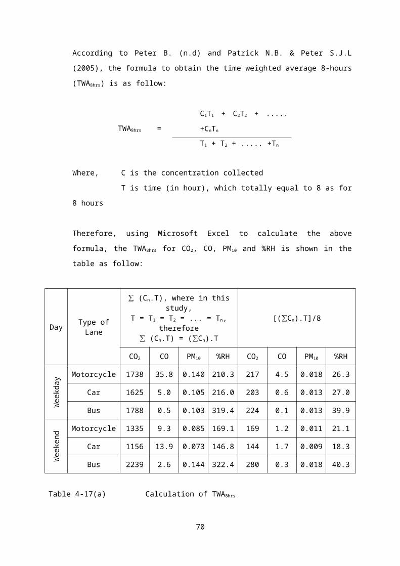
6.2 Conclusion

There are strong correlations between the numbers of vehicle with the pollutant. So

from this study it can conclude that the number of vehicle was influence the level of

pollutant at Immigration Station which means the emission from vehicle can move

into the inner setting of the station. However, reducing the number of vehicle crossing

this terminal wouldn’t bring any good especially to the economic sector. Engineering

controls such as installing passport self scanner at motorcycle and car lane,

separating drop off zone from the main entrance at the bus lane and regularly

maintain the cleanliness and efficiency of the mechanical ventilation air conditioning

(MVAC) operation not only reduced the amount of pollutant concentration in

Immigration Station but also enhance economic benefit and services value as this

can reduce the time lost of the operation and over paid to the substituted officer as

well as repairing the mechanical failure of the MVAC system. The control measure by

implementing administrative approach such as regulate the engine switched off for

motorcycle when arrive 50 meter from the passport examination booth like what have

been done in Singapore’s entry point, job rotation to reduce the exposure on single

person and awareness campaign of using personal protective equipment when

necessary.

70

REFERENCES

Ahmad Fadzil A.S., et-al. (2013). Air Pollution Study of Vehicles Emission In High Volume

Traffic: Selangor, Malaysia As A Case Study. WSEAS Transactions on Systems , 12

(2).

Asif F., et-al. (1996). Air Pollution from Motor Vehicles: Standards and Technologies for

Controlling Emissions. Washington: The World Bank.

Automobile Emission: An Overview. (n.d.).

Azliyana, A., et-al. (2011). Polycyclic Aromatic Hydrocarbons (PAHs) pollution from vehicle

emission in the environment of highway roadside in Johor, Malaysia. International

Conference on Biotechnology and Environment Management. 18. IACSIT Press,

Singapore.

Compedium of Environment Statistics Malaysia 2011. Department of Statistics Malaysia.

Compedium of Environment Statistics Malaysia 2013. Department of Statistics Malaysia.

Fisher, G.W., et-al. (2002). Health effect due to motor vehicle air pollution in New Zealand:

Report to the Ministry of Transport.

Guideline for Statistical Analysis of Occupationl Exposure Data. (1994). Retrieved from U.S.

Environmental Protection Agency:

http://www.epa.gov/oppt/exposure/pubs/stat_guide_occ.pdf

Harish, M. (2012). A study on air pollution by automobiles in Bangalore City. Management

Reaserch & Practice , 4 (3), 25-36.

Heinsohn R.J. & Cimbala J.M. (2003). Indoor Air Quality Engineering: Environmental Health

and Control of Indoor Pollutants. New York: Marcel Dekker.

71

Kirchstetter T.W. et al. (1999). On-road measurement of fine particles and nitrogen oxide

emission from light- and heavy-duty motor vehicles. Atmospheric Environment , 33

(18), 2955-2968.

Lund Research Ltd. (2013). Kruskal-Wallis H Test using SPSS Statistics. Retrieved from

Laerd Statistics: https://statistics.laerd.com/spss-tutorials/kruskal-wallis-h-test-using-

spss-statistics.php

Lund Research Ltd. (2013). Pearson's Product-Moment Correlation using SPSS. Retrieved

from Laerd Statistics: https://statistics.laerd.com/spss-tutorials/pearsons-product-

moment-correlation-using-spss-statistics.php

Malaysia Environmental Quality Report 2012. Department of Environment Malaysia.

Oliver L.H.L., et-al. (2012). Urban Air Environmental Health Indicators for Kuala Lumpur City.

Sains Malaysiana , 41 (2), 179-191.

Subramani, T. (2012). Study of air pollution due to vehicle emission in tourism centre.

International Journal of Engineering Research and Applications , 2 (3), 1753-1763.

Susanto, S. & Erni, S.T. (2005). Study on correlation between motor vehicle emission and

public health. Proceedings of the Eastern Asia Society for Transportation Studies , 5,

1841-1856.

Wan Hashim, W.I., & Nor Azam, R. A case study of mitigating air pollution emissions at

traffic light junctions. Human Settlement Development , II.

World Health Organization. (n.d.). Retrieved from Household (Indoor) Air Pollution:

http://www.who.int/indoorair/en/

World Health Organization. (2014, March). Retrieved from Ambient (outdoor) air quality and

health: http://www.who.int/mediacentre/factsheets/fs313/en/

72

mohdruhaizie.commohdruhaizie.com/hs223/hs223finalyear/fyp/fypsitimasha… · web viewthe main...

Documents