webinar11 network integration slides-with-notes2
TRANSCRIPT
8/10/2019 Webinar11 Network Integration Slides-With-Notes2
http://slidepdf.com/reader/full/webinar11-network-integration-slides-with-notes2 1/102
Page 1
Activity-Based Modeling
Session 11: Network Integration
Speakers: Joe Castiglione and Peter Vovsha August 30, 2012
TMIP Webinar Series
8/10/2019 Webinar11 Network Integration Slides-With-Notes2
http://slidepdf.com/reader/full/webinar11-network-integration-slides-with-notes2 2/102
Page 2
Activity-Based Modeling: Network Integration
AcknowledgmentsThis presentation was prepared through the collaborative efforts
of Resource Systems Group, Inc. and Parsons Brinckerhoff.
– Presenters
• Joe Castiglione and Peter Vovsha
– Moderator
• John Gliebe
– Content Development, Review and Editing • Joe Castiglione, Peter Vovsha, John Gliebe, Jason Chen, Joel
Freedman, Rosella Picado, John Bowman, Mark Bradley
– Media Production
• Bhargava Sana
2
Resource Systems Group and Parsons Brinckerhoff have developed these webinars
collaboratively, and we will be presenting each webinar together. Here is a list of the persons
involved in producing today’s session.
Joe Castiglione and Peter Vovsha are co-presenters. They were also primarily responsible
for preparing the material presented in this session.
John Gliebe is the session moderator.
Content development was also provided by John Gliebe, Jason Chen, Joel Freedman, and
Rosella Picado. John Bowman and Mark Bradley provided review. Bhargava Sana was responsible for media production, including setting up and managing
the webinar presentation

8/10/2019 Webinar11 Network Integration Slides-With-Notes2
http://slidepdf.com/reader/full/webinar11-network-integration-slides-with-notes2 3/102
Page 3
Activity-Based Modeling: Network Integration
2012 Activity-Based Modeling Webinar Series
Executive and Management Sessions
Executive Perspective February 2
Institutional Topics for Managers February 23
Technical Issues for Managers March 15
Technical Sessions
Activity-Based Model Framework April 5
Population Synthesis and Household Evolution April 26 Accessibility and Treatment of Space May 17
Long-Term and Medium Term Mobility Models June 7
Activity Pattern Generation June 28
Scheduling and Time of Day Choice July 19
Tour and Trip Mode, Intermediate Stop Location August 9
Network Integration August 30
Forecasting, Performance Measures and Software September 20
3
For your reference, here is a list of all of the webinars topics and dates that have been planned.
As you can see, we are presenting a different webinar every three weeks. Three weeks ago, we
covered the tenth topic in the series — Tour and Trip Mode, Intermediate Stop Location. This
session covered some of the key mode and destination choice components of the activity-based
model system.
Today’s session is the eighth of nine technical webinars, where we will cover the details of
activity-based model design and implementation. In today’s session, we will describe how
different activity-based model systems are integrated with network or supply models, and key
considerations of this linkage.
8/10/2019 Webinar11 Network Integration Slides-With-Notes2
http://slidepdf.com/reader/full/webinar11-network-integration-slides-with-notes2 4/102
Page 4
Activity-Based Modeling: Network Integration
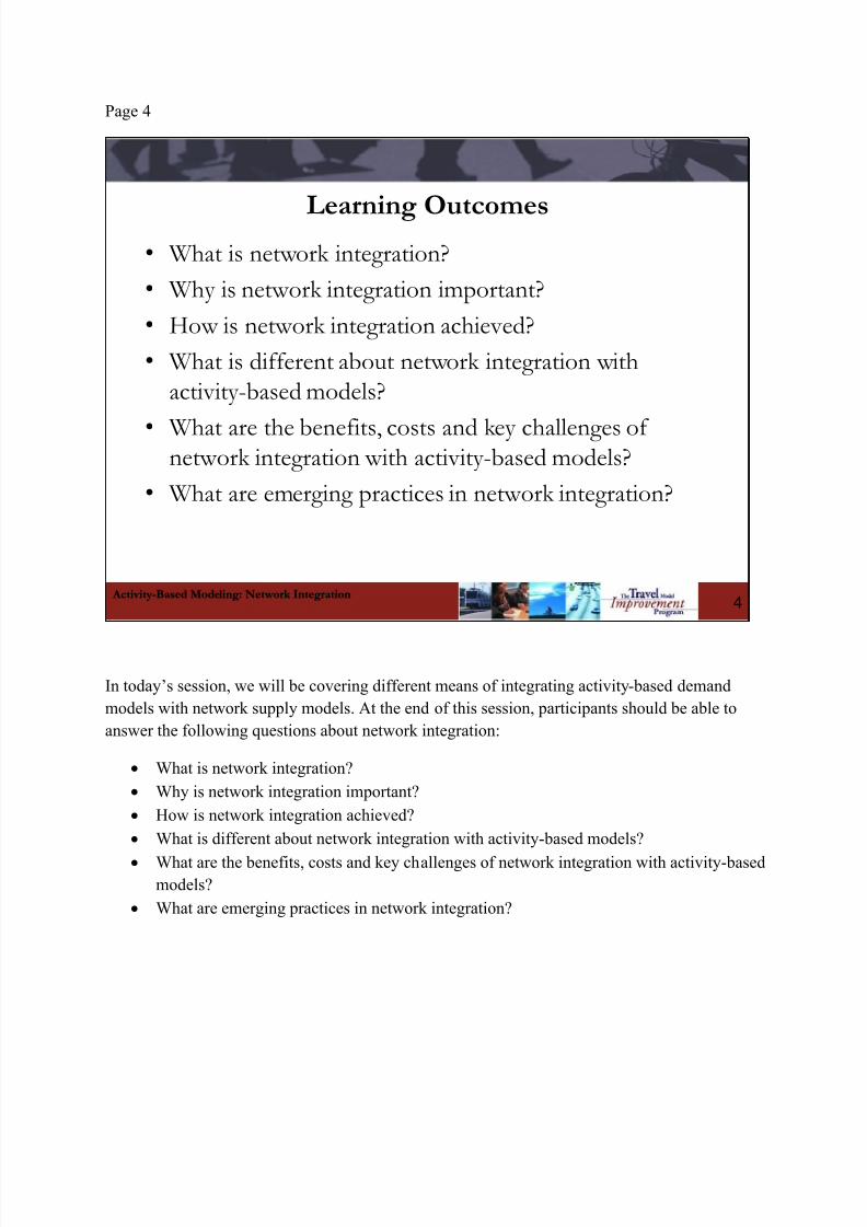
Learning Outcomes• What is network integration?
• Why is network integration important?
• How is network integration achieved?
• What is different about network integration with
activity-based models?
• What are the benefits, costs and key challenges ofnetwork integration with activity-based models?
• What are emerging practices in network integration?
4
In today’s session, we will be covering different means of integrating activity-based demand
models with network supply models. At the end of this session, participants should be able to
answer the following questions about network integration:
What is network integration?
Why is network integration important?
How is network integration achieved?
What is different about network integration with activity-based models?
What are the benefits, costs and key challenges of network integration with activity-basedmodels?
What are emerging practices in network integration?

8/10/2019 Webinar11 Network Integration Slides-With-Notes2
http://slidepdf.com/reader/full/webinar11-network-integration-slides-with-notes2 5/102
Page 5
Activity-Based Modeling: Network Integration
What do we mean by network integration?• A desired outcome:
– Network-derived level of service variables used to predict
destination, mode, and trip timing decisions are consistent
with the level of service predicted by the network assignment
• A system of program structures carefully designed to
achieve this outcome
– Decision modules, variable specifications, data structures,procedures
5
There are two senses in which we can use the term “network integration” First, the term can
refer to a condition or an outcome that is achieved when the network-derived level of service
variables used to predict activity generation, destination, mode, and trip timing decisions are
consistent with the level of service that results when these trips are loaded onto networks during
the network assignment steps. Second, the term can refer to the data structures and procedures
that are used to achieve this outcome.
8/10/2019 Webinar11 Network Integration Slides-With-Notes2
http://slidepdf.com/reader/full/webinar11-network-integration-slides-with-notes2 6/102
Page 6
Activity-Based Modeling: Network Integration
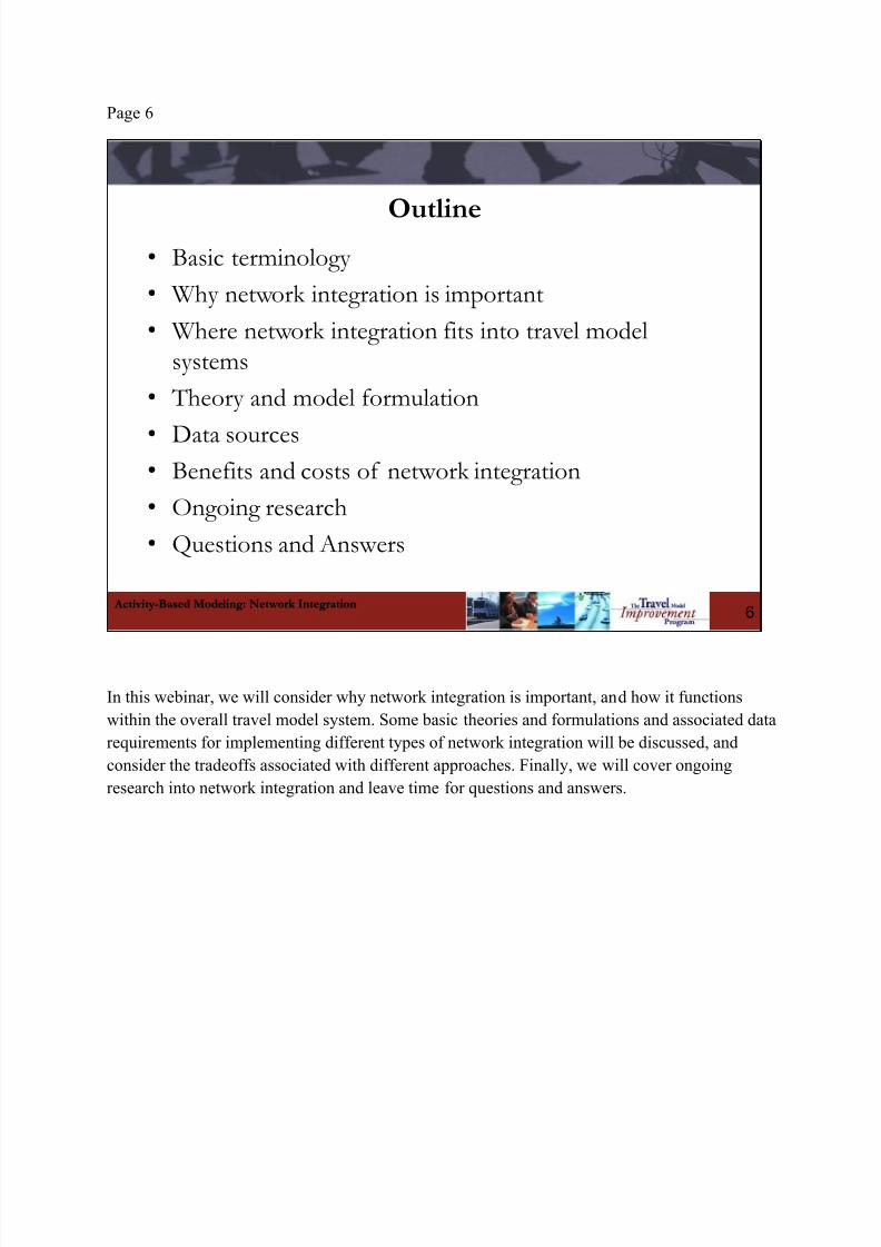
Outline• Basic terminology
• Why network integration is important
• Where network integration fits into travel model
systems
• Theory and model formulation
•Data sources
• Benefits and costs of network integration
• Ongoing research
• Questions and Answers
6
In this webinar, we will consider why network integration is important, and how it functions
within the overall travel model system. Some basic theories and formulations and associated data
requirements for implementing different types of network integration will be discussed, and
consider the tradeoffs associated with different approaches. Finally, we will cover ongoing
research into network integration and leave time for questions and answers.
8/10/2019 Webinar11 Network Integration Slides-With-Notes2
http://slidepdf.com/reader/full/webinar11-network-integration-slides-with-notes2 7/102
Page 7
Activity-Based Modeling: Network Integration
Terminology• Demand Models
• Supply Models
• Feedback
• Convergence
• Equilibrium
7
This slide shows basic terminology for that will be used in this session and other sessions.
Demand Models: Tools used to generate estimates of the type, amount, locations, mode
and timing of the demand for travel. Typically, this refers to the dimensions of travel that
are predicted by the first three steps of a traditional 4-step model (as distinct from the
final assignment step) or that predicted by an activity-based demand model. Demand
models can be basic or extremely complex.
Supply Models: Tools used to generate estimates network performance measures (such
as link flows and congested travel times) which are used as key inputs to demand models.Like demand models, supply models can be quite basic in their formulation or
significantly more complex.
Feedback: Refers to the process through which information generated “lower” in the
model system (such as congested travel times from network assignment) is used as direct
or indirect input the models “higher” in the model system (such as activity generation).

8/10/2019 Webinar11 Network Integration Slides-With-Notes2
http://slidepdf.com/reader/full/webinar11-network-integration-slides-with-notes2 8/102
The purpose of feedback is to ensure that the final model outputs are consistent with the
model system inputs and assumptions.
Convergence: The condition when the impedances or level-of-service measurements
used as the basis for accessibility measures and as key inputs to the destination and mode
choice models are approximately equal to the travel times and costs produced by the final
network assignment process. Convergence is necessary in order to ensure the behavioral
integrity of the model system, as is considered both with the context of the network
assignment process, as well the overall model system.
Equilibrium: Equilibrium typically refers to the condition where during the network
assignment no traveler can decrease travel effort by shifting to a new path. This is known
as user equilibrium, although other conditions such as system optimum can also be
pursued.
8/10/2019 Webinar11 Network Integration Slides-With-Notes2
http://slidepdf.com/reader/full/webinar11-network-integration-slides-with-notes2 9/102
Page 8
Activity-Based Modeling: Network Integration
Demand Models• Predict dimensions of travel demand (activity generation,
destination, mode)
• Comprised of linked demand model components
• May be applied at aggregate (zones) or disaggregate levels
(persons, HHs)
• Transportation supply availability and network performance
variables derived from supply model may appear in the utilityexpressions of any of these components
• Accessibility variables (simplified log-sums) typically used to
represent complex hierarchical travel choices
• Model components interact, causing second-order effects on
model components that do not use network variables directly
8
Demand models are tools used to generate estimates of the type, amount, locations, mode and
timing of the demand for travel. Typically, this refers to the dimensions of travel that are
predicted by the first three steps of a traditional 4-step model (as distinct from the final
assignment step) or that predicted by an activity-based demand model. Demand models can be
extremely basic (such a simple cross-classification trip generation model) or extremely complex
(such as an intra-household activity generation/coordination model). There are usually a series of
individual model sub-components that we refer to collectively as a single demand model – for
example, the trip or activity generation model component is distinct from the destination choice
or distribution model component, which is distinct from the mode choice model component.
These and other components are executed in sequence.
Demand models can be applied at an aggregate level, such as zones, as is in most traditional trip-
based models, or may be applied at the level of individual persons or households, as is the case in
activity-based models. Critical inputs to demand models are measures of transportation supply
availability and transportation system performance that are derived from the supply model. In

8/10/2019 Webinar11 Network Integration Slides-With-Notes2
http://slidepdf.com/reader/full/webinar11-network-integration-slides-with-notes2 10/102
some cases, these measures are used directly in the demand model components, while in other
cases the measures may be incorporated into accessibility measures and used indirectly in
demand model components.

8/10/2019 Webinar11 Network Integration Slides-With-Notes2
http://slidepdf.com/reader/full/webinar11-network-integration-slides-with-notes2 11/102
Page 9
Activity-Based Modeling: Network Integration
Network / Supply Models• Represent system capacity and level of service under
different levels of congestion
• Require details of demand (location, timing, mode)from demand model
• Network structures composed of links and nodes, withdemand loading points
• Link performance functions estimate congested traveltimes
• Tolls – convert monetary cost to travel time using valueof time estimates and add to link travel times
9
Tools used to generate estimates network performance (such as link flows and congested travel
times), which are used as key inputs to demand models. Supply models can be basic (such a
simple aggregate static equilibrium model) or more complex (such as a DTA or traffic micro-
simulation model that incorporates detailed operation attributes such as signal timing). Supply
models require as input information about travel demand, such as the locations, timing, and
modes used for travel. These estimates of demand are applied to representations of network
structures comprised at minimum of links and nodes but sometimes incorporating additional
network attributes which are used to predict the paths through the network that will be used to
satisfy this demand. In traditional static assignment supply models, mathematical functions are
used to estimate congested travel times given supply and demand inputs, although more recent
supply modeling techniques rely less on these “volume delay functions.” Because travelers’
choices are influenced not only by travel times but also by monetary costs, supply models should
be configured to convert these costs into travel times so that they can be incorporated into the
path-building procedure.

8/10/2019 Webinar11 Network Integration Slides-With-Notes2
http://slidepdf.com/reader/full/webinar11-network-integration-slides-with-notes2 12/102
Page 10
Activity-Based Modeling: Network Integration
Feedback • Use of outputs from a later (“lower”) model
component as input into an earlier (“higher”) modelcomponent
• Intended to ensure that the final model outputs areconsistent with the model system inputs andassumptions
• Extent of feedback and equilibration rules relate tostructure of model
• Necessary in both traditional trip-based models as wellas activity-based models
10
Feedback refers to the process through which information generated “lower” in the model system
(such as congested travel times from network assignment) is used as direct or indirect input the
models “higher” in the model system (such as activity generation). Feedback is important in both
traditional trip-based models as well as activity-based models in order to ensure that the final
model outputs are consistent with the model system inputs and assumptions. The exact nature of
this feedback is related to the structure of the model. For example, if in an activity-based model
system the activity generation component uses accessibility measures that reflect network
performance then the supply model outputs should be fed back to update these accessibility
measures before running any subsequent model components. However, if a traditional trip-based
model system incorporates no network performance measures or network-based accessibility
measures in trip generation or trip distribution, then it may only be necessary to feed-back
network performance information through the mode choice step.
8/10/2019 Webinar11 Network Integration Slides-With-Notes2
http://slidepdf.com/reader/full/webinar11-network-integration-slides-with-notes2 13/102
Page 11
Activity-Based Modeling: Network Integration
Convergence & Equilibrium• Convergence necessary to
– Ensure behavioral integrity of the model system
– Achieve consistent and repeatable results
• Two types of convergence in model system
– …to an equilibrium condition (network convergence)
– …to a stable condition (system convergence)
• System convergence is predicated on networkconvergence
11
Model convergence is necessary to ensure the behavioral integrity of the model system, and to
ensure that the results will be useful in a policy context. The network performance or level-of-
service measurements used as the basis for accessibility measures and as key inputs to demand
model components must be approximately equal to the travel times and costs produced by the
final network assignment process. In a travel model system, there are at least two types of
convergence that we need to consider: network convergence and system convergence. When we
talk about convergence, we are implicitly talking about convergence “to” something. Typically
this means for networks that we are converging to an equilibrium condition (usually a
deterministic user equilibrium where, for each time period-origin-destination combination all
used routes have equal travel times, and no unused route has a lower travel time). For the overall
model system, this usually means that we are converging to a stable solution (rather than an
optimal solution as in the network context). It should be noted that in the context of an integrated
demand and network simulation model system, an essential precondition for pursuing overall
model system convergence is establishing network assignment convergence.
8/10/2019 Webinar11 Network Integration Slides-With-Notes2
http://slidepdf.com/reader/full/webinar11-network-integration-slides-with-notes2 14/102
Page 12
Activity-Based Modeling: Network Integration
Importance of Network Integration• Behavioral
– Demand patterns produce supply cost
– Supply costs influence demand patterns
• Structural
– Demand models results are input to supply model
– Supply model results are input to demand model
• Practical
– Policy/investment choices must be informed by stable, repeatable results
– Exchange of consistent information required to produce stable,
repeatable results
12
Proper network integration is critical in trip-based model systems as well as in activity-based
model systems because in both types of model systems the “demand models” and the “supply
models” are mutually dependent. The demand model generates information about the origins,
destinations, modes, and timing of travel based, in part, on transportation network performance
indicators as such as travel times and costs and provides this travel information to the supply
model. The supply model assigns travel to transportation model networks and generates
information on network performance, which is then in turn fed back to the demand model.
This consistency and feedback between the demand and the supply components of the modelsystem is essential to ensuring that the model system is useful as a policy and investment
analysis tool. For example, attempts to assess the impacts of road-pricing strategies for
congestion relief will be misleading if the model system doesn’t accurately represent the
location, timing and intensity of delays – these delays arise both from the individual travel
choices predicted by the demand model as well as from the network performance predicted by
the supply model.
8/10/2019 Webinar11 Network Integration Slides-With-Notes2
http://slidepdf.com/reader/full/webinar11-network-integration-slides-with-notes2 15/102
Page 13
Activity-Based Modeling: Network Integration
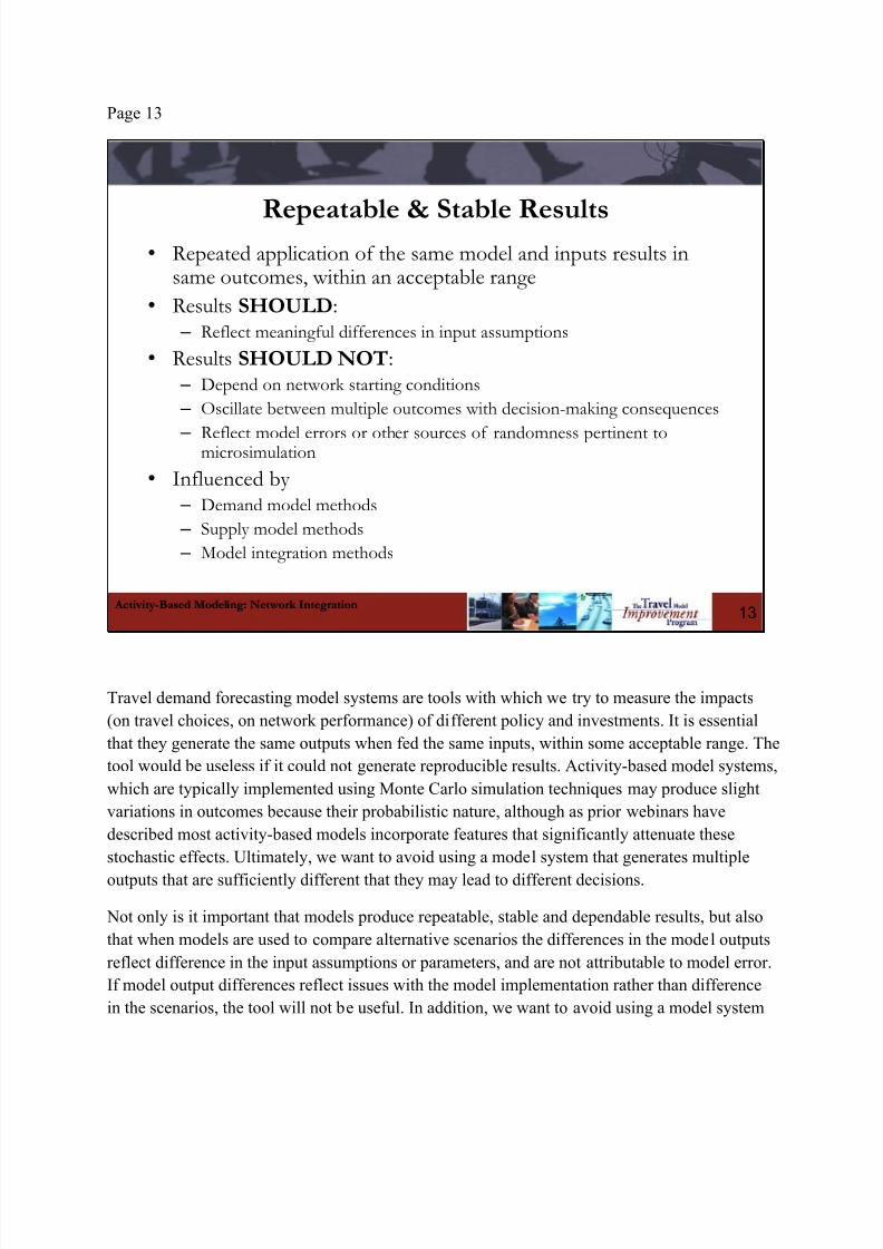
Repeatable & Stable Results• Repeated application of the same model and inputs results in
same outcomes, within an acceptable range
• Results SHOULD: – Reflect meaningful differences in input assumptions
• Results SHOULD NOT: – Depend on network starting conditions
– Oscillate between multiple outcomes with decision-making consequences
–
Reflect model errors or other sources of randomness pertinent tomicrosimulation
• Influenced by – Demand model methods
– Supply model methods
– Model integration methods
13
Travel demand forecasting model systems are tools with which we try to measure the impacts
(on travel choices, on network performance) of different policy and investments. It is essential
that they generate the same outputs when fed the same inputs, within some acceptable range. The
tool would be useless if it could not generate reproducible results. Activity-based model systems,
which are typically implemented using Monte Carlo simulation techniques may produce slight
variations in outcomes because their probabilistic nature, although as prior webinars have
described most activity-based models incorporate features that significantly attenuate these
stochastic effects. Ultimately, we want to avoid using a model system that generates multiple
outputs that are sufficiently different that they may lead to different decisions.
Not only is it important that models produce repeatable, stable and dependable results, but also
that when models are used to compare alternative scenarios the differences in the model outputs
reflect difference in the input assumptions or parameters, and are not attributable to model error.
If model output differences reflect issues with the model implementation rather than difference
in the scenarios, the tool will not be useful. In addition, we want to avoid using a model system

8/10/2019 Webinar11 Network Integration Slides-With-Notes2
http://slidepdf.com/reader/full/webinar11-network-integration-slides-with-notes2 16/102
that is dependent on the specifics of the network starting conditions, as this may thwart efforts to
produce repeatable results. For example, we want to our model system to produce similar final
results regardless of the “seed” impedances that we may use in the model systems initial
iteration. We also want to avoid using a model system where the results oscillate between
multiple outcomes in ways that may be consequential to decision making.
Our ability to produce repeatable and stable results is influenced by the resolution of the methods
used within both the demand and supply models, but is perhaps most crucially affected by the
methods we use to integrate our demand and supply models.

8/10/2019 Webinar11 Network Integration Slides-With-Notes2
http://slidepdf.com/reader/full/webinar11-network-integration-slides-with-notes2 17/102
Page 14
Activity-Based Modeling: Network Integration
Consistent Representation of Choices• Complex policy questions require simultaneous consideration of
demand and supply conditions
– Capacity improvements (release latent demand?)
– HOV lanes, tolling, and time-varying congesting pricing
– TDM policies, such as flexible work schedules
– Transit-oriented land use / compact growth
• Need to ensure that
– Change in network performance produces a theoreticallyplausible response in demand
– Change in demand produces a theoretically plausibleresponse in network performance
• Requires consistent representation of choices
14
When travel demand forecasting first emerged, the questions that practitioners asked of travel
models were simpler, such as how to size a given facility given the expected locations of future
populations and jobs. These days, decision-makers rely on travel demand models for answers to
more complex policy questions, and expect that these models are appropriately sensitive to the
complex behavioral responses.
For example, adding capacity to a roadway segment may not only result in diversion of traffic as
people seek reduced travel times, but might release latent demand that was suppressed due to
exiting congestion. Similarly, a pricing scenario might influence not only the use of specificroutes, but also timing and mode choices, destination choices, and even the generation of
activities.
And the complex policy questions are not strictly limited to transportation investments.
Decision-makers want travel models that are appropriately sensitive to the effects of compact,
mixed use, and transit-oriented land use. They want models that can help inform travel demand

8/10/2019 Webinar11 Network Integration Slides-With-Notes2
http://slidepdf.com/reader/full/webinar11-network-integration-slides-with-notes2 18/102
management strategies such as flexible work schedules. And (ideally) they want models that can
tell them who is impacted by these transportation and land use policy and investment decisions.
The complex questions necessitate models that appropriately and consistently capture the
relationship between travel demand and supply. If network pricing is to change by time-of-day,
then ideally network information (times, costs) at a time resolution consistent with this pricingscenario can be fed back from supply model to demand model. Similarly, if value-of-time
distribution information is used when predicting demand, then ideally this segmentation would
be reflected in the configuration of the supply model.

8/10/2019 Webinar11 Network Integration Slides-With-Notes2
http://slidepdf.com/reader/full/webinar11-network-integration-slides-with-notes2 19/102
Page 15
Activity-Based Modeling: Network Integration
Maintain Budgets & Constraints• No “extreme” behavior prevails
• Examples to avoid
– many people coming home really late… or working very
short days
– transferring 3 times… or walking long distances afterdisembarking from transit
– leaving young children stranded at school… or home alone
• Faithful to calibration targets
15
Related to the notion maintaining a consistent representation of choices between the demand and
network supply components of the model system is the issue of respecting temporal and spatial
constraints. Activity-based models contain intrinsic logic that already constrains individual travel
choices. For example, members of household that don’t own cars typically aren’t allowed to use
“drive alone” modes. People don’t drive home from work alone if they haven’t driven to their
work location. Travelers aren’t allowed to depart from a location that wasn’t the destination of
the prior trip.
Ideally, the supply component of the model system can reflect these constraints. For example,transit skims should have sufficient temporal detail that they can reflect the fact that after a
certain time transit service is significantly less frequent, and thus shouldn’t be considered as an
alternative. The transit network processing should discourage extreme behavior such as making
three or more transfers, or assuming long-walk egress.

8/10/2019 Webinar11 Network Integration Slides-With-Notes2
http://slidepdf.com/reader/full/webinar11-network-integration-slides-with-notes2 20/102
Maintaining budgets and constraints is not usually considered one of the primary challenges in
integrating activity-based demand models with current network supply models. However, as
network supply models incorporate ever increasing levels of temporal, spatial and behavioral
detail (such as the linked nature of trips on a tour), these issues may become more pronounced.

8/10/2019 Webinar11 Network Integration Slides-With-Notes2
http://slidepdf.com/reader/full/webinar11-network-integration-slides-with-notes2 21/102
Page 16
Activity-Based Modeling: Network Integration
Bridge Expansion Example• No Build Alternative
– 4 lanes (2 in each direction, no occupancy restrictions)
– No tolls
– Regional transit prices do not change by time of day
• Build Alternative(s)
– Add 1 lane in each direction (total of 6)
– New lanes will be HOV (peak period or all day?)
– Tolling (flat rate or time/congestion-based)
– Regional transit fares priced higher during peak periods
16
To understand the impacts of network integration, let’s revisit the example bridge expansion
transportation planning and policy project.
For this scenario analysis, we will be considering a number of alternatives: a no-build alternative
and a various configurations of the build alternative. In the no-build alternative the bridge has 4
lanes (2 in each direction), there are no tolls, and the transit fare stays the same all day. In the
various build alternatives, there are 6 lanes on the bridge. In some alternatives the two additional
lanes will be HOV lanes all day, while in other alternatives the two additional lanes will be HOV
lanes only during peak periods. In addition, in some build alternatives there will be a new tollthat is the same across the entire day, while in other build alternatives there will be a toll that will
be only applied during peak periods, or when certain levels of congestion occur. Finally, in the
build alternatives regional transit fares will be higher during peak periods.
How would the analysis of these alternatives be impacted by different network integration
schemes?

8/10/2019 Webinar11 Network Integration Slides-With-Notes2
http://slidepdf.com/reader/full/webinar11-network-integration-slides-with-notes2 22/102
Page 17
Activity-Based Modeling: Network Integration
Bridge Expansion Mobility Effects
17
Work location may
change due to tolls or
new HOV and transitlanes
New school locations may be
possible due to changes in
traffic using the new bridgeVehicle ownership may
decrease with tolls or new
HOV and transit options
Vehicle type may change to
take advantage of fuel
efficient vehicle toll
reductions
Owning a transponder may
encourage more use of the
bridge
Owning a
transit pass
may increase
with new
transit lanes
Previous presentations have described the potential long-term and medium-term effects of the
bridge expansion, such as changes in the usual work and school locations, changes in levels of
vehicle ownership, and the types of vehicles owned, and changes in the transit pass or toll
transponder adoption.
8/10/2019 Webinar11 Network Integration Slides-With-Notes2
http://slidepdf.com/reader/full/webinar11-network-integration-slides-with-notes2 23/102
Page 18
Activity-Based Modeling: Network Integration
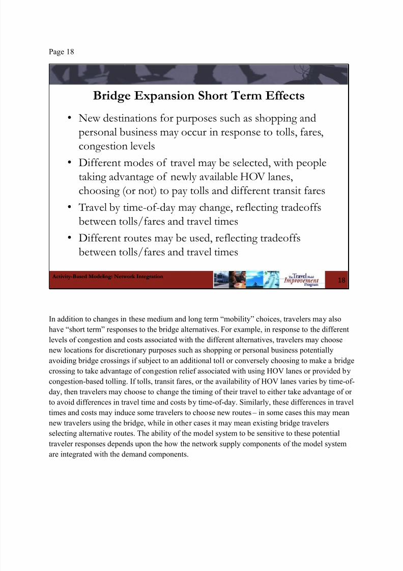
Bridge Expansion Short Term Effects• New destinations for purposes such as shopping and
personal business may occur in response to tolls, fares,congestion levels
• Different modes of travel may be selected, with peopletaking advantage of newly available HOV lanes,choosing (or not) to pay tolls and different transit fares
• Travel by time-of-day may change, reflecting tradeoffsbetween tolls/fares and travel times
• Different routes may be used, reflecting tradeoffsbetween tolls/fares and travel times
18
In addition to changes in these medium and long term “mobility” choices, travelers may also
have “short term” responses to the bridge alternatives. For example, in response to the different
levels of congestion and costs associated with the different alternatives, travelers may choose
new locations for discretionary purposes such as shopping or personal business potentially
avoiding bridge crossings if subject to an additional toll or conversely choosing to make a bridge
crossing to take advantage of congestion relief associated with using HOV lanes or provided by
congestion-based tolling. If tolls, transit fares, or the availability of HOV lanes varies by time-of-
day, then travelers may choose to change the timing of their travel to either take advantage of or
to avoid differences in travel time and costs by time-of-day. Similarly, these differences in travel
times and costs may induce some travelers to choose new routes – in some cases this may mean
new travelers using the bridge, while in other cases it may mean existing bridge travelers
selecting alternative routes. The ability of the model system to be sensitive to these potential
traveler responses depends upon the how the network supply components of the model system
are integrated with the demand components.
8/10/2019 Webinar11 Network Integration Slides-With-Notes2
http://slidepdf.com/reader/full/webinar11-network-integration-slides-with-notes2 24/102
Page 19
Activity-Based Modeling: Network Integration
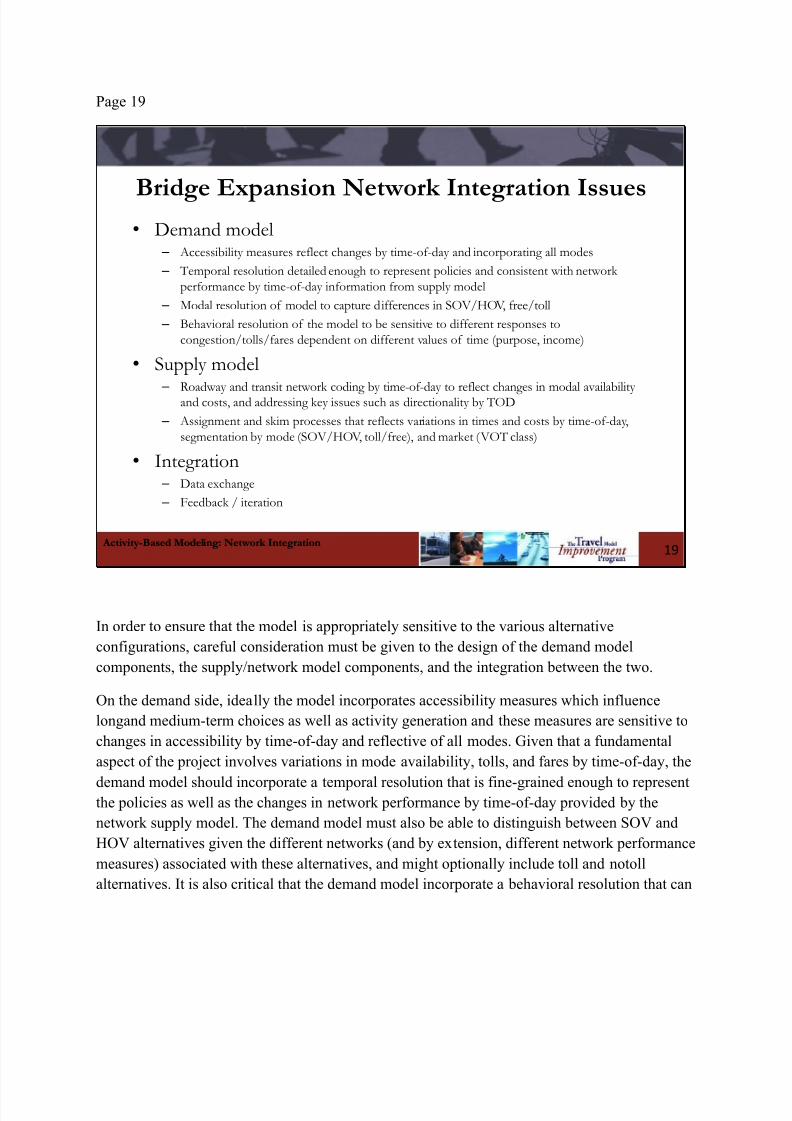
Bridge Expansion Network Integration Issues• Demand model
– Accessibility measures reflect changes by time-of-day and incorporating all modes
– Temporal resolution detailed enough to represent policies and consistent with network
performance by time-of-day information from supply model
– Modal resolution of model to capture differences in SOV/HOV, free/toll
– Behavioral resolution of the model to be sensitive to different responses to
congestion/tolls/fares dependent on different values of time (purpose, income)
• Supply model –
Roadway and transit network coding by time-of-day to reflect changes in modal availabilityand costs, and addressing key issues such as directionality by TOD
– Assignment and skim processes that reflects variations in times and costs by time-of-day,
segmentation by mode (SOV/HOV, toll/free), and market (VOT class)
• Integration – Data exchange
– Feedback / iteration
19
In order to ensure that the model is appropriately sensitive to the various alternative
configurations, careful consideration must be given to the design of the demand model
components, the supply/network model components, and the integration between the two.
On the demand side, ideally the model incorporates accessibility measures which influence
longand medium-term choices as well as activity generation and these measures are sensitive to
changes in accessibility by time-of-day and reflective of all modes. Given that a fundamental
aspect of the project involves variations in mode availability, tolls, and fares by time-of-day, the
demand model should incorporate a temporal resolution that is fine-grained enough to representthe policies as well as the changes in network performance by time-of-day provided by the
network supply model. The demand model must also be able to distinguish between SOV and
HOV alternatives given the different networks (and by extension, different network performance
measures) associated with these alternatives, and might optionally include toll and notoll
alternatives. It is also critical that the demand model incorporate a behavioral resolution that can

8/10/2019 Webinar11 Network Integration Slides-With-Notes2
http://slidepdf.com/reader/full/webinar11-network-integration-slides-with-notes2 25/102
reflect different sensitivities to congestion, tolls and fares depending on the traveler, travel
purpose and other travel attributes.
On the supply side, the roadway and transit networks should incorporate information about
modal availability (such as HOV lanes) as well as about how the network configurations and
costs change by time of day, consistent with the policies to be evaluated – will tolls or fares varyonly by broad multi-hour time period, or will they vary by finer time periods such as individual
hours? A key aspect of this is directionality, especially for transit transit networks need to be
coded to reflect the true level of service provided by direction. In order to exploit the modal and
time period information coded in the networks and provide relevant information to the demand
model, it is also critical to ensure that the network assignment and network skim methods reflect
the variations in times and costs by time-of-day, mode and potentially other dimensions such as
value of time.
Finally, the core issues of integration also need to be considered – what information is being
exchanged between the demand and supply components, and how are the demand and supplycomponents interacting in an iterative feedback framework in order to ensure consistent and
reasonable results? The demand model must provide information about travel demand that is
sufficiently segmented by mode, time-of-day, traveler class and other attributes, while the
supply model must provide information about network performance that is similarly segmented.
8/10/2019 Webinar11 Network Integration Slides-With-Notes2
http://slidepdf.com/reader/full/webinar11-network-integration-slides-with-notes2 26/102
Page 20
Activity-Based Modeling: Network Integration
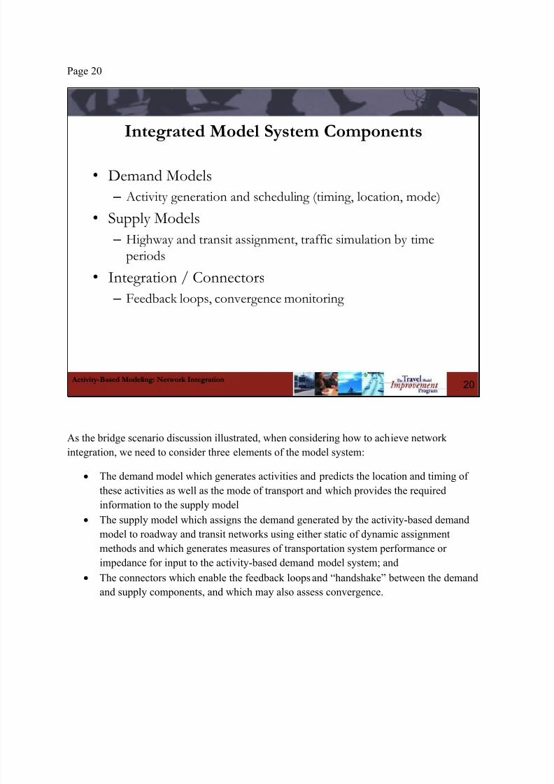
Integrated Model System Components
• Demand Models
– Activity generation and scheduling (timing, location, mode)
• Supply Models
– Highway and transit assignment, traffic simulation by timeperiods
• Integration / Connectors – Feedback loops, convergence monitoring
20
As the bridge scenario discussion illustrated, when considering how to achieve network
integration, we need to consider three elements of the model system:
The demand model which generates activities and predicts the location and timing of
these activities as well as the mode of transport and which provides the required
information to the supply model
The supply model which assigns the demand generated by the activity-based demand
model to roadway and transit networks using either static of dynamic assignment
methods and which generates measures of transportation system performance orimpedance for input to the activity-based demand model system; and
The connectors which enable the feedback loops and “handshake” between the demand
and supply components, and which may also assess convergence.

8/10/2019 Webinar11 Network Integration Slides-With-Notes2
http://slidepdf.com/reader/full/webinar11-network-integration-slides-with-notes2 27/102
Page 21
Activity-Based Modeling: Network Integration
Typical Integrated Model System Flow
21
Demand Model
Estimates of
demand by
location, time
period, mode,
etc.
Supply Model
Estimates of
network
performance by
location, time
period, mode, etc.
Are skims and
demand
consistent or
max iteration
reached?
Feedback Process
Revised estimates
of network
performance by
location, time
period, mode, etc.
END
NO
YES
This figure illustrates the relationships amongst the three types of components in the integrated
model system. Note that this figure is relevant regardless of whether the demand model is a more
typical aggregate, trip-based model or a disaggregate activity based model. It illustrates that the
demand model uses travel time and cost information in the form of skims, in addition to other
attributes associated with travelers (such as income) and locations (such as the amount of
employment) to predict activity-travel events.
The network supply models then apply this demand to roadway and transit networks to estimate
volumes and associated times and costs. This new time and cost information is then used todevelop updated skims. These new skims are then used to rerun the demand model to predict a
revised set of activity-travel events and again this demand is assigned to roadway and transit
networks to develop revised estimates of volumes, times and costs. The convergence of the
model system to a stable solution is assessed, typically using measures that consider changes in
the demand flows by geography or by changes in the skims, and if a pre-specified threshold is
met, the process terminates.

8/10/2019 Webinar11 Network Integration Slides-With-Notes2
http://slidepdf.com/reader/full/webinar11-network-integration-slides-with-notes2 28/102
If the threshold is not met, then the demand and network supply models are run again,
convergence is checked, and the process repeats until either the threshold is met or the system
reaches a maximum number of iterations.
8/10/2019 Webinar11 Network Integration Slides-With-Notes2
http://slidepdf.com/reader/full/webinar11-network-integration-slides-with-notes2 29/102
Page 22
Activity-Based Modeling: Network Integration
More Choice Dimensions• More model system components
– Activity generation
– Tour and stop location
– Tour and trip mode
– Time-of-day
• System components are more complex
– Incorporate constraints (time of day, mode)
– Incorporate fine-grained resolution (behavioral, temporal, spatial)
• Linkages amounted system components are more detailed
– Types of information
– Amount of information
22
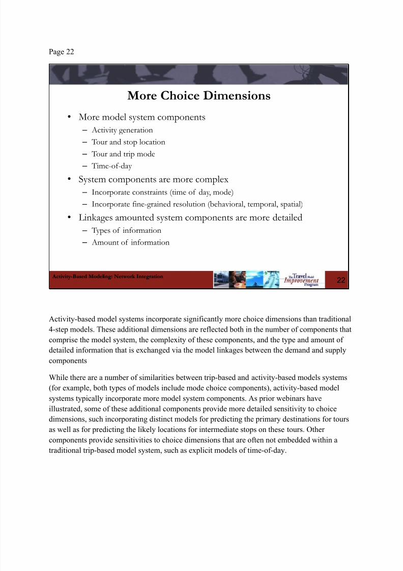
Activity-based model systems incorporate significantly more choice dimensions than traditional
4-step models. These additional dimensions are reflected both in the number of components that
comprise the model system, the complexity of these components, and the type and amount of
detailed information that is exchanged via the model linkages between the demand and supply
components
While there are a number of similarities between trip-based and activity-based models systems
(for example, both types of models include mode choice components), activity-based model
systems typically incorporate more model system components. As prior webinars haveillustrated, some of these additional components provide more detailed sensitivity to choice
dimensions, such incorporating distinct models for predicting the primary destinations for tours
as well as for predicting the likely locations for intermediate stops on these tours. Other
components provide sensitivities to choice dimensions that are often not embedded within a
traditional trip-based model system, such as explicit models of time-of-day.

8/10/2019 Webinar11 Network Integration Slides-With-Notes2
http://slidepdf.com/reader/full/webinar11-network-integration-slides-with-notes2 30/102
Activity-based model components are also typically more complex than traditional trip-based
model systems. For example, AB model components may explicitly incorporate information
about constraints, such as the time windows available to individuals to participate in activities, or
the maximum distance than can be travelled within an available time window. And of course,activity-based models systems employ higher levels of behavioral, temporal and even spatial
detail, using individual persons and householders as decision-makers, representing time in small
time slices such as one-hour, half-hour, or even continuously.
The fine-grained behavioral, temporal, and spatial resolution of activity-based demand models
and the complexity of the models that exploit this detail require that significant consideration be
given to the coding the linkages between demand model system components. There are two
primary linkages in an activity-based model system: from the demand model to the network
supply model, and from the network supply model to the demand model.
8/10/2019 Webinar11 Network Integration Slides-With-Notes2
http://slidepdf.com/reader/full/webinar11-network-integration-slides-with-notes2 31/102
Page 23
Activity-Based Modeling: Network Integration23
Trip generation
Trip distribution
Mode choice
Time-of-day factoring
Network assignment
s k i m s
Long-term choices(vehavl, work/school location)
Destination choices
Mode choice
Time-of-day choices
Network assignment
S k i m s / l o g s um s
Mobility choices(transit pass ownership)
Activity generation
Demand Model Network Supply ModelTrip-Based Model Activi ty-Based Model
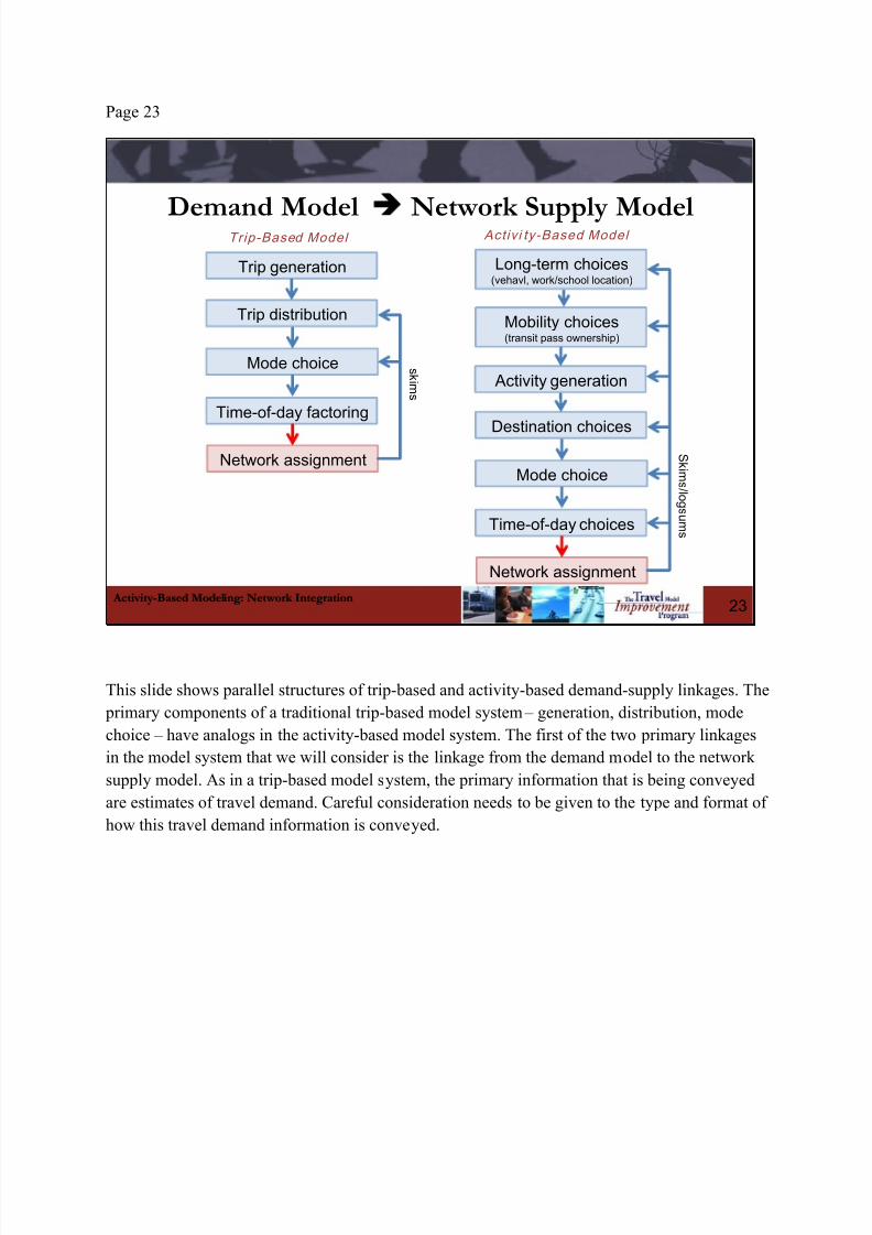
This slide shows parallel structures of trip-based and activity-based demand-supply linkages. The
primary components of a traditional trip-based model system – generation, distribution, mode
choice – have analogs in the activity-based model system. The first of the two primary linkages
in the model system that we will consider is the linkage from the demand model to the network
supply model. As in a trip-based model system, the primary information that is being conveyed
are estimates of travel demand. Careful consideration needs to be given to the type and format of
how this travel demand information is conveyed.
8/10/2019 Webinar11 Network Integration Slides-With-Notes2
http://slidepdf.com/reader/full/webinar11-network-integration-slides-with-notes2 32/102
Page 24
Activity-Based Modeling: Network Integration
Market Segmentation• Overall travel market is comprised of submarkets
• Activity-based models provide more flexibility andefficiency in handling market segmentation
• Submarkets are differentiated by key attributes, such as:
– Mode
– Time-period
– Value-of-time
24
Trip Rate
Low IncomeHousehold
0 VehicleVehicle Less
than Workers
Drive alone Shared Ride Walk to Bus…
Vehicle morethan Workers
MediumIncome
Household
0 Vehicle…
High IncomeHousehold
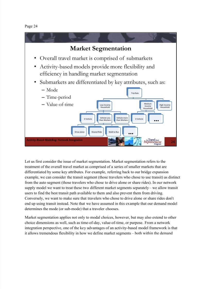
Let us first consider the issue of market segmentation. Market segmentation refers to the
treatment of the overall travel market as comprised of a series of smaller markets that are
differentiated by some key attributes. For example, referring back to our bridge expansion
example, we can consider the transit segment (those travelers who chose to use transit) as distinct
from the auto segment (those travelers who chose to drive alone or share rides). In our network
supply model we want to treat these two different market segments separately – we allow transit
users to find the best transit path available to them and also prevent them from driving.
Conversely, we want to make sure that travelers who chose to drive alone or share rides don’t
end up using transit instead. Note that we have assumed in this example that our demand model
determines the mode (or sub-mode) that a traveler chooses.
Market segmentation applies not only to modal choices, however, but may also extend to other
choice dimensions as well, such as time-of-day, value-of-time, or purpose. From a network
integration perspective, one of the key advantages of an activity-based model framework is that
it allows tremendous flexibility in how we define market segments – both within the demand

8/10/2019 Webinar11 Network Integration Slides-With-Notes2
http://slidepdf.com/reader/full/webinar11-network-integration-slides-with-notes2 33/102
model, within the network supply model, and in the linkages between these two components. In a
trip-based model system we have less flexibility to define market segments, primarily due to the
fact that as we increase the number of market segments there is a combinatorial effect that may
lead to the proliferation of a huge number of segments, each of which may require the
maintenance of multiple matrices regardless of how “big” the market segment truly is.

8/10/2019 Webinar11 Network Integration Slides-With-Notes2
http://slidepdf.com/reader/full/webinar11-network-integration-slides-with-notes2 34/102
Page 25
Activity-Based Modeling: Network Integration
Activity Trip Lists & Segmentation
25
• Trip tables not produced until assignment step, more flexibly specified
• Trip lists may be converted to trip tables by aggregating over multiple dimensions
– Time of day
– Activity types
– Person types
– occupancy class
– Transit submode /access mode
– Other… EZ pass, transit and parking pass holders, etc.
In contrast to the proliferation of matrices and all the associated computation and storage
challenges that results from increased market segmentation in a traditional matrix-based and trip-
based model system, activity-based model systems support much more flexible market
segmentation due to the “list- based” nature of the activity-based demand model simulation. One
of the outputs from the activity-based demand model is a list of trips that contains all the detailed
spatial, temporal, behavioral, and socio-demographic information associated with the trip and
traveler.
When assigning travel, most network supply models require as input a set of origin-destinationmatrices segmented by mode and time-of-day. The detailed information contained in the list-
based activity-based demand model can be aggregated to virtually any market segmentation. For
example, if a user wanted to transition from using a three hour peak period assignment to 3
separate 1-hour peak hour assignments or to assign by value of time class, they only need to
revise the aggregation process and make associated changes to the network supply model
assignment and skim scripts.
8/10/2019 Webinar11 Network Integration Slides-With-Notes2
http://slidepdf.com/reader/full/webinar11-network-integration-slides-with-notes2 35/102
Page 26
Activity-Based Modeling: Network Integration
Highway Market Segmentation
26
Choice
Auto
Drive
alone
GP(1)
Pay(2)
Shared
ride 2
GP(3)
HOV(4)
Pay(5)
Shared
ride 3+
GP(6)
HOV(7)
Pay(8)
Non-
motorized
Walk(9)
Bike(10)
Transit
Walk
access
Local
bus(11)
Express
bus(12)
BRT(13)
LRT(14)
Commuter
rail(15)
PNR
access
Local
bus(16)
Express
bus(17)
BRT(18)
LRT(19)
Commuter
rail(20)
KNR
access
Local
bus(21)
Express
bus(22)
BRT(23)
LRT(24)
Commuter
rail(25)
School
Bus(26)
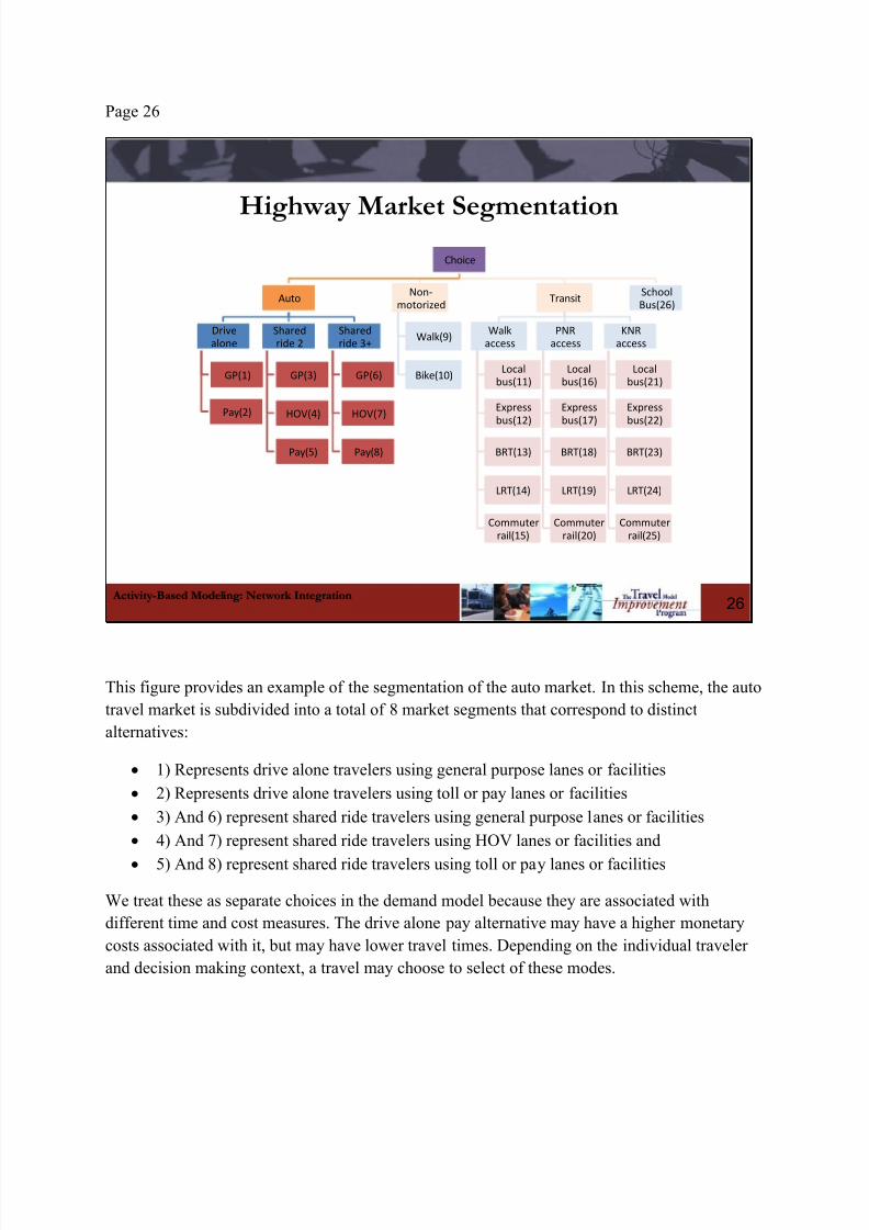
This figure provides an example of the segmentation of the auto market. In this scheme, the auto
travel market is subdivided into a total of 8 market segments that correspond to distinct
alternatives:
1) Represents drive alone travelers using general purpose lanes or facilities
2) Represents drive alone travelers using toll or pay lanes or facilities
3) And 6) represent shared ride travelers using general purpose lanes or facilities
4) And 7) represent shared ride travelers using HOV lanes or facilities and
5) And 8) represent shared ride travelers using toll or pay lanes or facilities
We treat these as separate choices in the demand model because they are associated with
different time and cost measures. The drive alone pay alternative may have a higher monetary
costs associated with it, but may have lower travel times. Depending on the individual traveler
and decision making context, a travel may choose to select of these modes.

8/10/2019 Webinar11 Network Integration Slides-With-Notes2
http://slidepdf.com/reader/full/webinar11-network-integration-slides-with-notes2 36/102
In establishing the integration with the network supply model, we want to consider this as a
separate market segment because each choice may be subject to different opportunities or
constraints. For example, if the mode chose for a given trip is “drive alone- pay” then when we
assign this using the network supply model we can allow the trip to use pay/toll facilities as well
as general purpose lanes. However, we also want to restrict this trip from using HOV lanes.
8/10/2019 Webinar11 Network Integration Slides-With-Notes2
http://slidepdf.com/reader/full/webinar11-network-integration-slides-with-notes2 37/102
Page 27
Activity-Based Modeling: Network Integration
Transit Market Segmentation
27
Choice
Auto
Drive alone
GP(1)
Pay(2)
Shared ride
2
GP(3)
HOV(4)
Pay(5)
Shared ride
3+
GP(6)
HOV(7)
Pay(8)
Non-
motorized
Walk(9)
Bike(10)
Transit
Walk
access
Local
bus(11)
Express
bus(12)
BRT(13)
LRT(14)
Commuter
rail(15)
PNR
access
Local
bus(16)
Express
bus(17)
BRT(18)
LRT(19)
Commuter
rail(20)
KNR
access
Local
bus(21)
Express
bus(22)
BRT(23)
LRT(24)
Commuter
rail(25)
School
Bus(26)
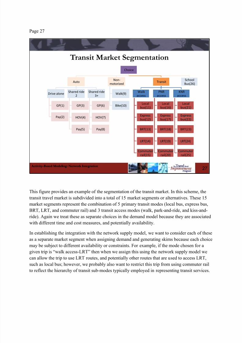
This figure provides an example of the segmentation of the transit market. In this scheme, the
transit travel market is subdivided into a total of 15 market segments or alternatives. These 15
market segments represent the combination of 5 primary transit modes (local bus, express bus,
BRT, LRT, and commuter rail) and 3 transit access modes (walk, park-and-ride, and kiss-and-
ride). Again we treat these as separate choices in the demand model because they are associated
with different time and cost measures, and potentially availability.
In establishing the integration with the network supply model, we want to consider each of these
as a separate market segment when assigning demand and generating skims because each choicemay be subject to different availability or constraints. For example, if the mode chosen for a
given trip is “walk access-LRT” then when we assign this using the network supply model we
can allow the trip to use LRT routes, and potentially other routes that are used to access LRT,
such as local bus; however, we probably also want to restrict this trip from using commuter rail
to reflect the hierarchy of transit sub-modes typically employed in representing transit services.
8/10/2019 Webinar11 Network Integration Slides-With-Notes2
http://slidepdf.com/reader/full/webinar11-network-integration-slides-with-notes2 38/102
Page 28
Questions and Answers
28

8/10/2019 Webinar11 Network Integration Slides-With-Notes2
http://slidepdf.com/reader/full/webinar11-network-integration-slides-with-notes2 39/102
Page 29
Activity-Based Modeling: Network Integration
Network Supply Model Demand Model
29
Trip generation
Trip distribution
Mode choice
Time-of-day factoring
Network assignment
s k i m s
Long-term choices(vehavl, work/school location)
Destination choices
Mode choice
Time-of-day choices
Network assignment
S k i m s / l o g s um s
Mobility choices(transit pass ownership)
Activity generation
This slide shows parallel structures of trip-based and activity-based supply-demand linkages. The
second key linkage in the activity-based model system that we will consider is the linkage from
the network supply model back to the demand model.
As in a trip-based model system, the primary information that is being conveyed are estimates of
network performance such as travel times and costs, often referred to as network “skims”. This
feedback of skims is critical to achieving the converged or stable model results that are necessary
for the model to be useful as an analytic tool. As with the demand model to network supply
model linkage, careful consideration needs to be given to how this network performanceinformation is fed back and incorporated into the activity-based demand model component.
8/10/2019 Webinar11 Network Integration Slides-With-Notes2
http://slidepdf.com/reader/full/webinar11-network-integration-slides-with-notes2 40/102
Page 30
Activity-Based Modeling: Network Integration
Network Performance (LOS) Measures in Activity-Based Model Components
• Auto ownership and other mobility attributes
• Activity pattern generation
• Destination and mode/occupancy choice
• Time of day choice
• Intra-household joint tour frequency choice
30
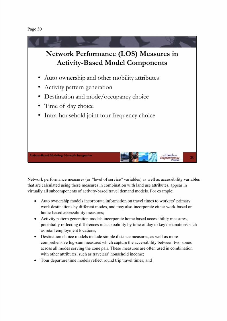
Network performance measures (or “level of service” variables) as well as accessibility variables
that are calculated using these measures in combination with land use attributes, appear in
virtually all subcomponents of activity-based travel demand models. For example:
Auto ownership models incorporate information on travel times to workers’ primary
work destinations by different modes, and may also incorporate either work-based or
home-based accessibility measures;
Activity pattern generation models incorporate home based accessibility measures,
potentially reflecting differences in accessibility by time of day to key destinations suchas retail employment locations;
Destination choice models include simple distance measures, as well as more
comprehensive log-sum measures which capture the accessibility between two zones
across all modes serving the zone pair. These measures are often used in combination
with other attributes, such as travelers’ household income;
Tour departure time models reflect round trip travel times; and

8/10/2019 Webinar11 Network Integration Slides-With-Notes2
http://slidepdf.com/reader/full/webinar11-network-integration-slides-with-notes2 41/102
Intra-household joint tour frequency models have incorporated retail accessibility
measures.
8/10/2019 Webinar11 Network Integration Slides-With-Notes2
http://slidepdf.com/reader/full/webinar11-network-integration-slides-with-notes2 42/102
Page 31
Activity-Based Modeling: Network Integration
Trip-based Assignment/Skim Time Periods• Minimum assignment periods (small urban areas)
– AM Peak and/or PM Peak highway assignment (2-3 hours ofdemand)
• Sometimes transposing one to represent the other
– Mid-day off-peak highway assignment (5-6 hours of demand) – Often no transit assignment, or AM Peak only – No non-motorized assignment
• More typical assignment periods (medium-large urban
areas) – AM Peak, PM Peak, Mid-day off-peak highway assignment – Sometimes evening off-peak highway assignment – Peak/Off-peak transit assignment
• AM peak transposed to represent PM peak
– No non-motorized assignment
31
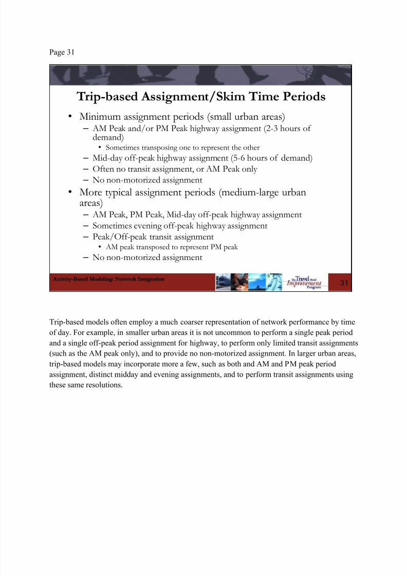
Trip-based models often employ a much coarser representation of network performance by time
of day. For example, in smaller urban areas it is not uncommon to perform a single peak period
and a single off-peak period assignment for highway, to perform only limited transit assignments
(such as the AM peak only), and to provide no non-motorized assignment. In larger urban areas,
trip-based models may incorporate more a few, such as both and AM and PM peak period
assignment, distinct midday and evening assignments, and to perform transit assignments using
these same resolutions.
8/10/2019 Webinar11 Network Integration Slides-With-Notes2
http://slidepdf.com/reader/full/webinar11-network-integration-slides-with-notes2 43/102
Page 32
Activity-Based Modeling: Network Integration
Assignment /Skim Time Periods• Ideally, want time period resolution to be consistent across
demand and network supply components, but challenges with:
• Generating, storing, accessing large LOS matrices• Using small time periods with static assignment (DTA better)
• More detailed assignment and skim periods provide bettermodel sensitivity
•
Time period definitions should reflect potential policyapplications• Consideration of variable tolls, reversible lanes, transit service differentials
• Function of network size, complexity, population/demand• Larger areas, more complex systems – congestion spreading across
longer time periods
32
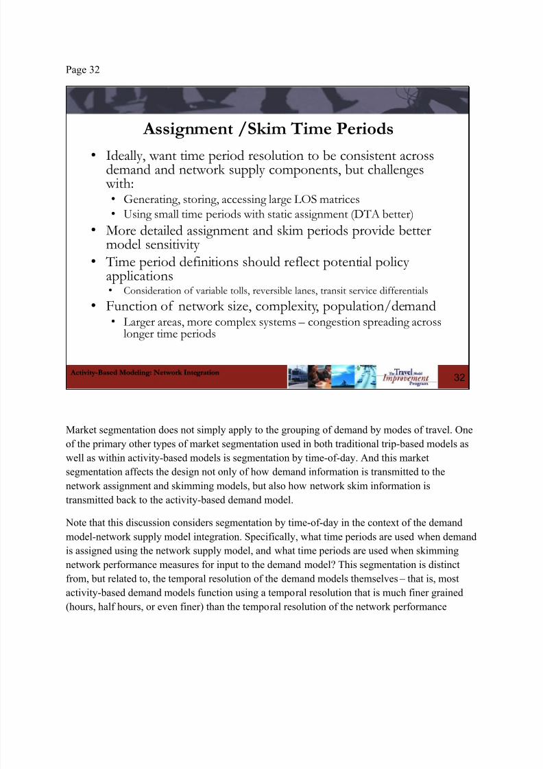
Market segmentation does not simply apply to the grouping of demand by modes of travel. One
of the primary other types of market segmentation used in both traditional trip-based models as
well as within activity-based models is segmentation by time-of-day. And this market
segmentation affects the design not only of how demand information is transmitted to the
network assignment and skimming models, but also how network skim information is
transmitted back to the activity-based demand model.
Note that this discussion considers segmentation by time-of-day in the context of the demand
model-network supply model integration. Specifically, what time periods are used when demandis assigned using the network supply model, and what time periods are used when skimming
network performance measures for input to the demand model? This segmentation is distinct
from, but related to, the temporal resolution of the demand models themselves – that is, most
activity-based demand models function using a temporal resolution that is much finer grained
(hours, half hours, or even finer) than the temporal resolution of the network performance
8/10/2019 Webinar11 Network Integration Slides-With-Notes2
http://slidepdf.com/reader/full/webinar11-network-integration-slides-with-notes2 44/102
indicators input to the models. Achieving consistency in temporal resolution across demand and
supply models is a key current research topic.
Ideally, in order to have the greatest sensitivity in the integrated demand-network supply model
system, we would input to the demand model information about network performance generated
by the supply model that is consistent with the temporal resolution of the demand model, and wewould assign this demand to model networks using this same temporal resolution. However,
theoretical and practical concerns necessitate simplification – the runtimes and hardware
requirements associated with generating, storing, and accessing network skims for detailed time
periods quickly become onerous, and the using static assignment methods for short time periods
may be problematic. Some of these issues may be addressed by using DTA, which we will
discuss later in this presentation.
Practically, we need to consider a few issues:
Our assignment time periods and assignment skim periods should be consistent; More detailed assignment and skim periods provide better model system sensitivity,
particularly to changes by time of day and mode;
Time period definitions should reflect potential policy applications – it won’t be possible
to test the impacts of hourly changes in tolls, fares, reversible lanes unless information at
this level of temporal detail can be generated by the network supply model for input to
the demand model; and
Time period definitions should reflect the regional context – larger regions with more
complex transportation systems may be more subject to phenomena such as peak
spreading, or may have more diverse modal alternatives with service differential by
detailed time of day.
8/10/2019 Webinar11 Network Integration Slides-With-Notes2
http://slidepdf.com/reader/full/webinar11-network-integration-slides-with-notes2 45/102
Page 33
Activity-Based Modeling: Network Integration
Modules & Feedback Pathways – 4 Step
33
Trip generation
Trip distribution
Mode choice
Time-of-day factoring
Network assignment
s k i m
s
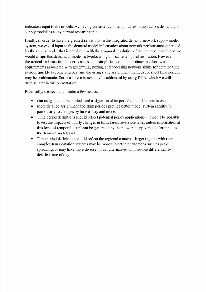
Most typical 4-step travel model systems do not incorporate explicit time-of-day models. Rather,
a set of fixed factors (potentially segmented by purpose and mode) are applied post-mode choice
that transform daily production-attraction format trip matrices into origin-destination trip
matrices by time period.
Applying time-of-day factors to the trip tables at this point in the model system is a
simplification that makes it possible to generate assignment results by time-of-day, but without
requiring the proliferation of matrices that would result from incorporating time of day choice
models, or even from applying fixed time of day factors earlier in the model stream.
However, the use of time-of-day factors represents a significant compromise in the sensitivity of
the model system. For example, the model would be unable to respond to the time-of-day
changes that might result from the expansion or reduction of capacity in a congested corridor.
The model would also not be sensitive to the fact that as congesting increases, travelers start to
use the “shoulders” of the peak – known as peak spreading. And perhaps most significantly,

8/10/2019 Webinar11 Network Integration Slides-With-Notes2
http://slidepdf.com/reader/full/webinar11-network-integration-slides-with-notes2 46/102
there is no information on how these factors should change in the future given more demand. In
this last example, the use of fixed base year factors in the future year might significantly over-
estimate the amount of congestion encountered by travelers, and thus lead to unrealistic
responses by other model system components.
Some trip-based models do incorporate peak spreading models that begin to capture some of thesensitivity of travelers to changing the timing of their trips. However, such features are not
“typical” components of 4-step trip-based model.

8/10/2019 Webinar11 Network Integration Slides-With-Notes2
http://slidepdf.com/reader/full/webinar11-network-integration-slides-with-notes2 47/102
Page 34
Activity-Based Modeling: Network Integration
Modules & Feedback Pathways – ABM
34
Long-term choices(vehavl, work/school location)
Destination choices
Mode choice
Time-of-day choices
Network assignment
S k i m s / l o g s um s
Mobility choices(transit pass ownership)
Activity generation
In contrast to trip-based models, most activity-based models employ more detailed time period
information when integrating the demand and network supply components of the model system.
Some of the earliest activity-based models systems implemented in the United States used
relatively aggregate time periods for skimming and assignment, even when the demand models
operating using quite detailed time-of-day models.

8/10/2019 Webinar11 Network Integration Slides-With-Notes2
http://slidepdf.com/reader/full/webinar11-network-integration-slides-with-notes2 48/102
Page 35
Activity-Based Modeling: Network Integration
Assignment/Skim Segmentation Examples• SFCTA
– 6 time periods used in skimming and assignment (temporal resolution ofthe demand component are same broad time periods)
– Detailed auto and transit sub-modes
– Detailed zone structure
• CMAP – 8 time periods used in assignment and skimming (temporal resolution of
demand component is half-hour) – Detailed auto and transit sub-modes
• SACOG – 12 time periods in skimming and assignment (temporal resolution of
model is half-hour)
– Detailed auto and transit submodes
– Network skimming and assignment at zone level, enhanced with parcel-level geographic information
35
In contrast to trip-based models, most activity-based models employ more detailed time period
information when integrating the demand and network supply components of the model system.
Some of the earliest activity-based models systems implemented in the United States used
relatively aggregate time periods for skimming and assignment, even when the demand models
operating using quite detailed time-of-day models.
For example, the MORPC demand model uses 1-hour time periods when generating and
scheduling activities, but only employs two time periods when feeding back skim information to
the demand model. In contrast, the SFCTA integrated model system uses a consistent set of time periods for generating and scheduling activities, and for network assignment and skimming, but
these time periods are much broader than one hour. The recent updates to the SACOG model
have resulted in an implementation in which the demand model uses half-hour time periods for
generating and scheduling activities, and uses 12 time periods for network assignment and
skimming (hourly during the peaks, and broader time periods during the midday and
evening/night).

8/10/2019 Webinar11 Network Integration Slides-With-Notes2
http://slidepdf.com/reader/full/webinar11-network-integration-slides-with-notes2 49/102
All of the models described above incorporated fairly detailed auto and transit sub-model
alternatives in the demand model, and an analogous market segmentation in the demand and
network supply model linkages. In a sense, we can also consider the representation of space in
the model system as a type of geographic segmentation.
8/10/2019 Webinar11 Network Integration Slides-With-Notes2
http://slidepdf.com/reader/full/webinar11-network-integration-slides-with-notes2 50/102
Page 36
Activity-Based Modeling: Network Integration
More Assignment Strategies• Multiple time periods representing AM/PM Peaks,
shoulders before and after peaks, evening off-peaks,overnight off-peaks – CMAP (8 time periods)
• Multiple transit assignment periods--AM Peak, PM Peak,Mid-day – NYMTC (4 periods parallel to highway assignments)
– CMAP (8 periods parallel to highway assignments)
• Non-motorized assignment first attempts: – SFCTA & Portland
• VOT classes in addition to vehicle type and occupancy – CMAP Pricing ABM
36
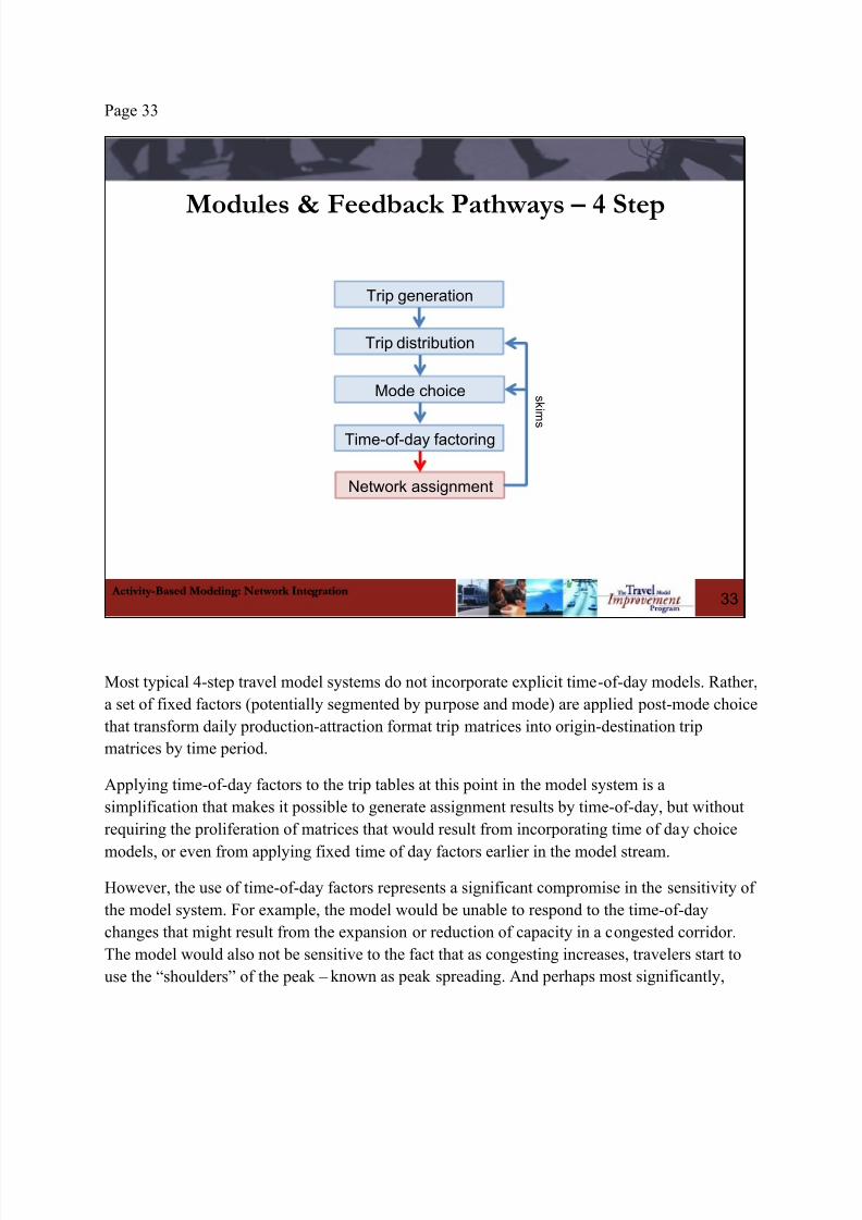
In general, there is a pronounced move towards incorporating greater levels of temporal detail in
both roadway and transit assignment and skimming, as evidenced by recent work in Chicago,
New York, Sacramento, and other regions.
In addition to the detailed segmentation by time of day, some advanced activity-based demand
and network supply model integration efforts are incorporating more advanced assignment and
skimming approaches that included non-motorized modes such as bikes, or that include roadway
assignments and skimming that incorporate value-of-time segmentation to capture different time
and cost tradeoffs.
8/10/2019 Webinar11 Network Integration Slides-With-Notes2
http://slidepdf.com/reader/full/webinar11-network-integration-slides-with-notes2 51/102
Page 37
Activity-Based Modeling: Network Integration
CMAP Multi-Class Assignment ClassesVehicle Type &
Value-Of-Time
Non-
toll
SOV
Non-toll
HOV2
Non-toll
HOV3+
Toll
SOV
Toll HOV2 Toll
HOV3+
Auto + external +
airport low VOT
1 3 5 2 4 6
Auto + external +
airport high VOT
7 9 11 8 10 12
Commercial 13 14
Light truck 15 16
Medium truck 17 18
Heavy truck 19 20
37
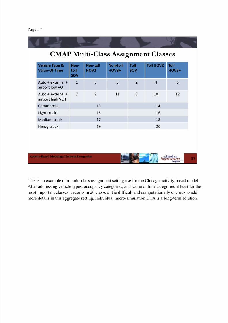
This is an example of a multi-class assignment setting use for the Chicago activity-based model.
After addressing vehicle types, occupancy categories, and value of time categories at least for the
most important classes it results in 20 classes. It is difficult and computationally onerous to add
more details in this aggregate setting. Individual micro-simulation DTA is a long-term solution.
8/10/2019 Webinar11 Network Integration Slides-With-Notes2
http://slidepdf.com/reader/full/webinar11-network-integration-slides-with-notes2 52/102
Page 38
Activity-Based Modeling: Network Integration
Differences in Accessing Skim Information• Trip-based models access skims in limited ways-usually just
destination and mode choice; time of day choice if present
– Matrix processing enables efficient access of skim values for large
batches of trips in a single operation (full OD loop)
• Activity-based models are based on individual micro-simulation
–
Rather than looping on all ODs for skim access and use, needselected skims within the loop over millions of individual records
– Many more model components use skims
– Computationally challenging
• Much greater memory requirements with efficient random access
• Some pre-computing of accessibility log-sums necessary
38
An interesting implementation issue relates to differences in the way that activity-based models
access and use skims relative to trip-based models. First, trip based models do not typically use
skims as comprehensively throughout the model system as activity-based models. Of course,
mode choice models use skims, and distribution models typically do as well. In the rare instances
where a trip-based model incorporates a time-of-day component then this model will also use
skims. But trip-based models are implemented within a matrix framework, looping first on
origins and then over destinations. This approach allows for efficient access to skim values for
large batches of trips in a single operation.
In contrast, activity-based models incorporate skim information throughout virtually all
components of the entire model system – destination choice, mode choice, time of day choice,
and in the generation of accessibility measures used as input to activity generation. Due to the
agent-based micro-simulation framework in which the activity-based model is applied, random
access of skims during the simulation is required. This is computationally challenging, and
necessitates much greater memory requirements, and efficient means of retrieving the skim data.
8/10/2019 Webinar11 Network Integration Slides-With-Notes2
http://slidepdf.com/reader/full/webinar11-network-integration-slides-with-notes2 53/102
Page 39
Activity-Based Modeling: Network Integration
Input Data Source Needs• Consistent treatment of time and space in ABMs reflects realistic
availability constraints
• Need data on changes in network supply by time-of-day – HOV lane status
– Reversible lanes – Variable road pricing – Transit service headways, fares and coverage
• Maintaining roadway supply by time-of-day is relatively
straightforward• Maintaining transit supply by time-of-day can be onerous, and
simplifying assumptions frequently made (i.e. PM supplyimpedances are a transpose of AM)
• New promising sources of network information andtechnologies (NavTech, GoogleTransit)
39
The input network supply data needed to integrate with an activity-based model system are not
significantly different than required to integrate with a traditional trip based model, but more
temporal and modal detail is typically required. A key advantage of activity-based models is that
they provide a framework for the consistent treatment of time and space and reflect realistic
availability constraints. To maintain consistency with and provide good information to the
activity-based demand model, the network supply model should ideally also incorporate detailed
information on network supply, particularly by time-of-day. This should include information on
changes in capacity by time-of-day, such as the presence of HOV and reversible lanes, and
transit service headways fares and coverage. Coding and maintaining information about roadway
supply by time of day is relatively straightforward as this information can usually be simply
coded as an attribute on a common base network. Coding and maintaining information on transit
supply by time-of-day can be considerably more onerous due to the significant numbers of
variations in transit route alignments and service levels. For example, a single transit route may
have a number of patterns with different termini and service frequencies. In some cases, agencies

8/10/2019 Webinar11 Network Integration Slides-With-Notes2
http://slidepdf.com/reader/full/webinar11-network-integration-slides-with-notes2 54/102
have developed detailed transit network by time of day, while in other instances simplifying
assumptions are made, such as PM transit service as a transpose of AM service.
8/10/2019 Webinar11 Network Integration Slides-With-Notes2
http://slidepdf.com/reader/full/webinar11-network-integration-slides-with-notes2 55/102
8/10/2019 Webinar11 Network Integration Slides-With-Notes2
http://slidepdf.com/reader/full/webinar11-network-integration-slides-with-notes2 56/102
Page 41
Activity-Based Modeling: Network Integration
Transit Network Structures
41
transit access linkstransit route
zone/centroid
connectors
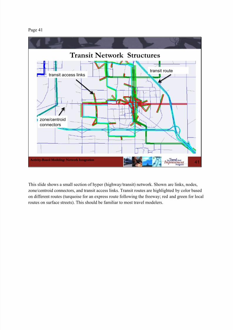
This slide shows a small section of hyper (highway/transit) network. Shown are links, nodes,
zone/centroid connectors, and transit access links. Transit routes are highlighted by color based
on different routes (turquoise for an express route following the freeway; red and green for local
routes on surface streets). This should be familiar to most travel modelers.

8/10/2019 Webinar11 Network Integration Slides-With-Notes2
http://slidepdf.com/reader/full/webinar11-network-integration-slides-with-notes2 57/102
Page 42
Activity-Based Modeling: Network Integration
Network Validation Needs• Network supply model outputs
• Level of service skims• Link volumes / speeds / times
• Calibration / validation needs• Good data coverage critical• More temporal detail, possibly more spatial, vehicle class, facility
type detail
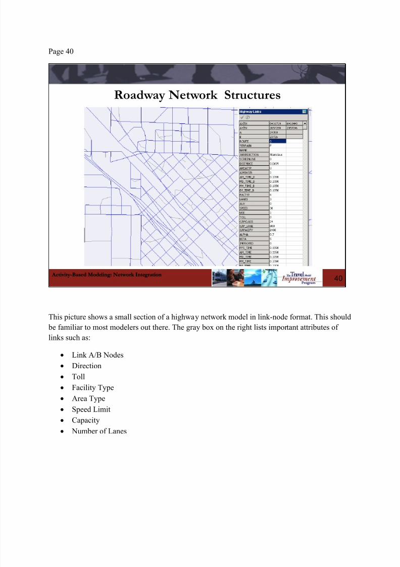
• Similar measures to trip-based models• Counts, screenlines• VMT / VHT• Speeds, travel times – archived ITS data
• Transit boardings / alightings• Transit ridership by line
• Parking lot utilization rates
42
We’ve been discussing the network skims as a critical output of the network supply model
because it is the information contained within these skims that make the model system truly
integrated, where each component is informing the other. However, most practitioners are also
interested in other key outputs from the network supply model, link and segment-based volumes
and speeds. To assess how well both the network supply model as well as the overall demand-
supply model system are performing, it is critical to have a robust model validation dataset. In
general, the types of measures used to validate an integrated activity-based travel demand model
systems are very similar to those used to validate a traditional trip-based models: a distribution
of counts and speeds across different locations, facility types and vehicle classes, as well as
transit boardings, alightings, and loads. The most significant difference is that these validation
data are ideally available at a level of temporal detail that are consistent with the time periods
used in the network assignment model. This may presents a minor additional burden as the time
period detail is greater than that used in most trip-based models. In addition, there are also some
validation data related to model components unique to the activity-based model system, such as
park-and-ride lot utilization.
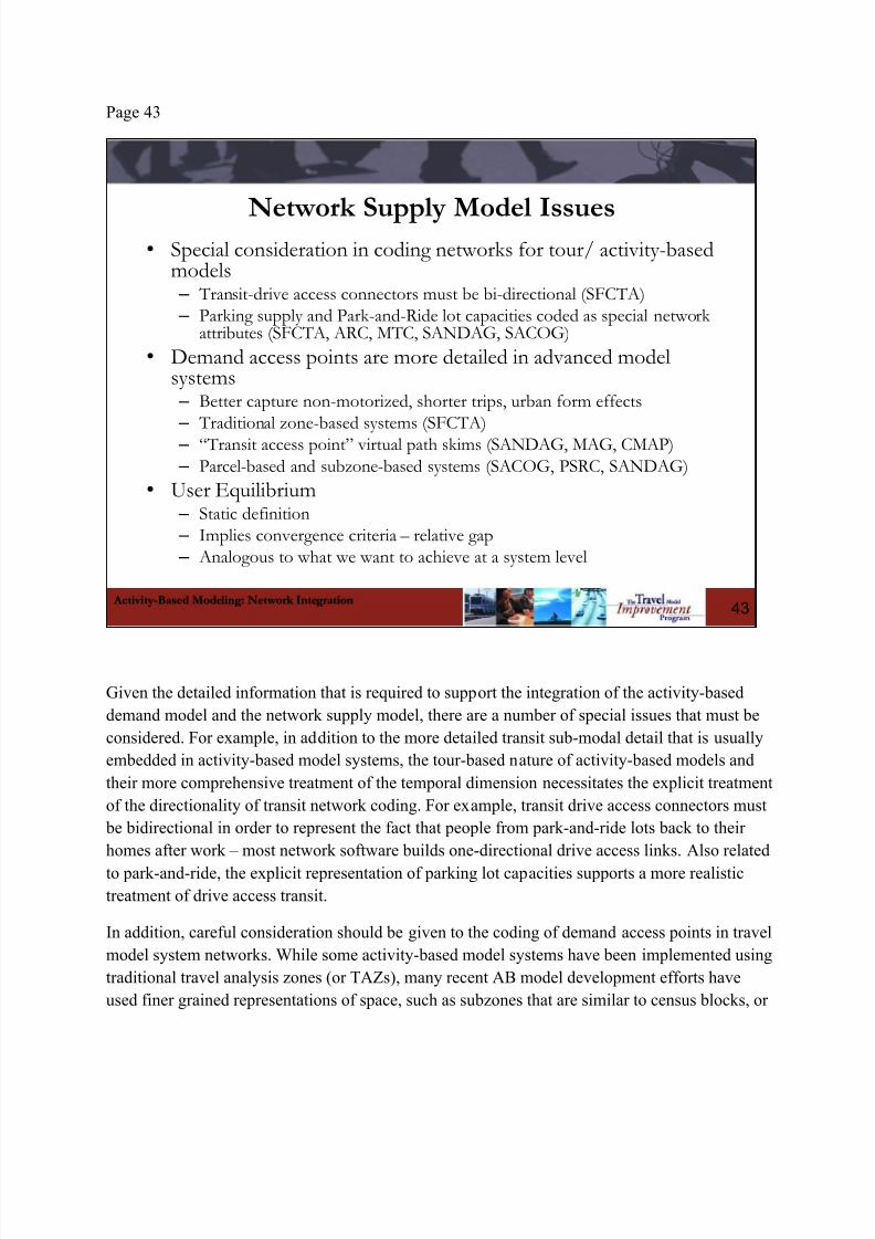
8/10/2019 Webinar11 Network Integration Slides-With-Notes2
http://slidepdf.com/reader/full/webinar11-network-integration-slides-with-notes2 58/102
Page 43
Activity-Based Modeling: Network Integration
Network Supply Model Issues• Special consideration in coding networks for tour/ activity-based
models – Transit-drive access connectors must be bi-directional (SFCTA)
– Parking supply and Park-and-Ride lot capacities coded as special networkattributes (SFCTA, ARC, MTC, SANDAG, SACOG)
• Demand access points are more detailed in advanced modelsystems – Better capture non-motorized, shorter trips, urban form effects
– Traditional zone-based systems (SFCTA)
– “Transit access point” virtual path skims (SANDAG, MAG, CMAP)
– Parcel-based and subzone-based systems (SACOG, PSRC, SANDAG)
• User Equilibrium – Static definition
– Implies convergence criteria – relative gap
– Analogous to what we want to achieve at a system level
43
Given the detailed information that is required to support the integration of the activity-based
demand model and the network supply model, there are a number of special issues that must be
considered. For example, in addition to the more detailed transit sub-modal detail that is usually
embedded in activity-based model systems, the tour-based nature of activity-based models and
their more comprehensive treatment of the temporal dimension necessitates the explicit treatment
of the directionality of transit network coding. For example, transit drive access connectors must
be bidirectional in order to represent the fact that people from park-and-ride lots back to their
homes after work – most network software builds one-directional drive access links. Also related
to park-and-ride, the explicit representation of parking lot capacities supports a more realistic
treatment of drive access transit.
In addition, careful consideration should be given to the coding of demand access points in travel
model system networks. While some activity-based model systems have been implemented using
traditional travel analysis zones (or TAZs), many recent AB model development efforts have
used finer grained representations of space, such as subzones that are similar to census blocks, or

8/10/2019 Webinar11 Network Integration Slides-With-Notes2
http://slidepdf.com/reader/full/webinar11-network-integration-slides-with-notes2 59/102
actual parcels. In addition, some model systems simultaneously use multiple levels of geography
that reflect transit, roadway and non-motorized impedances; however, in most cases the network
components of these model systems do not directly used this same detailed geography. The
relationships between different levels of spatial resolution in the model system should be
explicit.
Finally, most of the following discussion assumes the use of an activity-based model system
integrated with a traditional static network assignment model that converges to a static user
equilibrium solution. Other assignment methodologies may also be used in connection with
activity-based models, and the final section of this webinar considers current research linking
activity-based model systems with dynamic traffic assignment models.
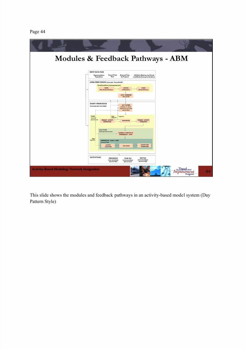
8/10/2019 Webinar11 Network Integration Slides-With-Notes2
http://slidepdf.com/reader/full/webinar11-network-integration-slides-with-notes2 60/102
Page 44
Activity-Based Modeling: Network Integration
Modules & Feedback Pathways - ABM
44
INPUT DATA FILES
LONG-TERM CHOICE (once per household)
SHORT-TERM CHOICE
(once per pe rson-day)
OUTPUT FILES
Usual Locations (once per person)
WORK
(Non-Student Workers)
SCHOOL
(All Students)
WORK
(Student Workers)
AUTO OWNERSHIP
(Household)
DAY PATTERN
(activities & home-
based tours for eachperson-day)
PRIMARY ACTIVITY
DESTINATION
MAIN MODE PRIMARY ACTIVITY
SCHEDULING
NUMBER & PURPOSE OF
INTERMEDIATE STOPS
ACTIVITY
LOCATIONTRIP MODE
ACTIVITY/TRIP
SCHEDULING
TOURS
(once per
person-tour)
Aggr.Logsums
Aggr.Logsums
Logsums
HALF-TOURS
(twice per person-tour)
INTERMEDIATE STOPS & TRIPS
(once per trip)
RepresentativePopulation
Parcel/PointData
External Tripsby Purpose
LOS Skim Matrices, by Periodand Mode (from prior iteration)
TRIP FILE(one record per
person-trip)
TOUR FILE(one record per
person-tour
PERSON FILE(one record per
person-day
This slide shows the modules and feedback pathways in an activity-based model system (Day
Pattern Style)
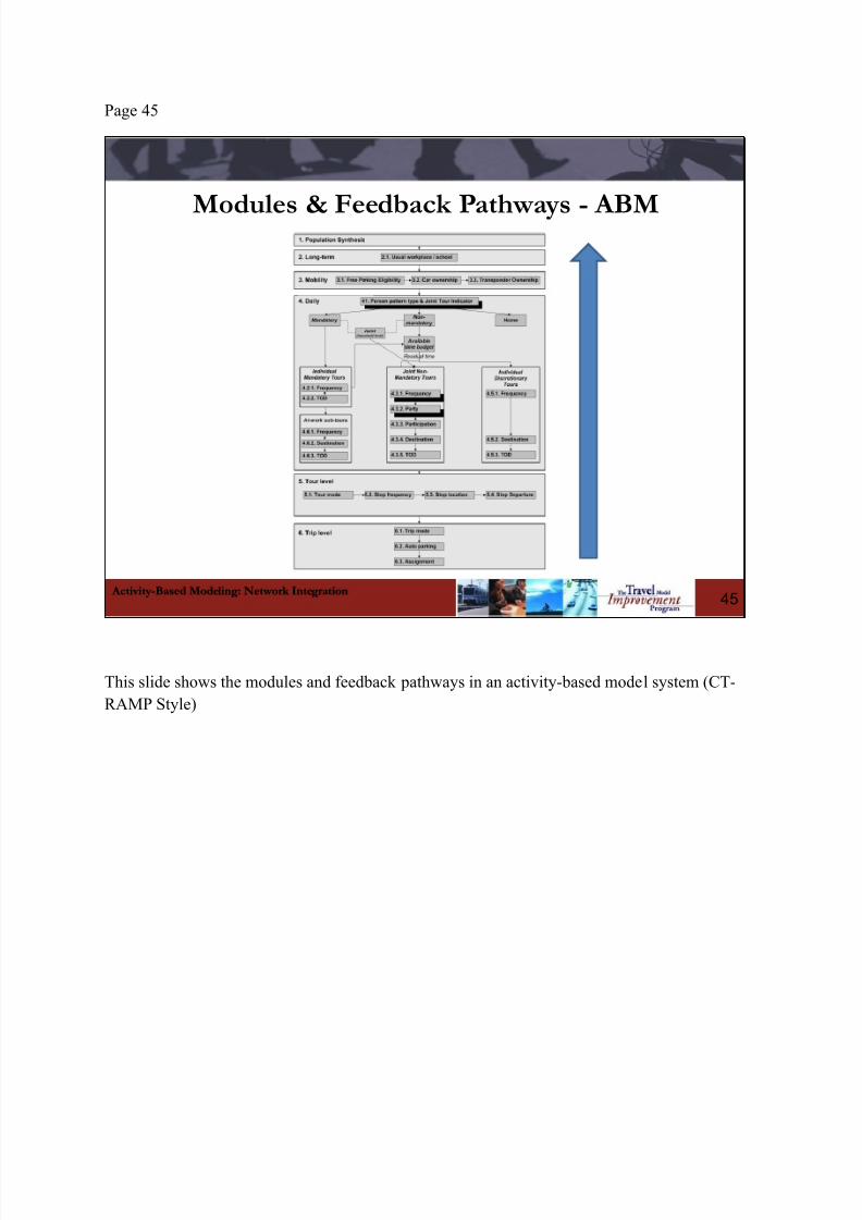
8/10/2019 Webinar11 Network Integration Slides-With-Notes2
http://slidepdf.com/reader/full/webinar11-network-integration-slides-with-notes2 61/102
Page 45
Activity-Based Modeling: Network Integration
Modules & Feedback Pathways - ABM
45
This slide shows the modules and feedback pathways in an activity-based model system (CT-
RAMP Style)
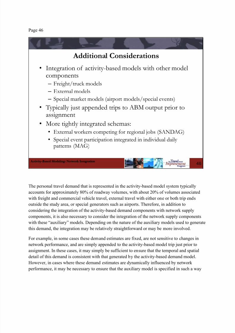
8/10/2019 Webinar11 Network Integration Slides-With-Notes2
http://slidepdf.com/reader/full/webinar11-network-integration-slides-with-notes2 62/102
Page 46
Activity-Based Modeling: Network Integration
Additional Considerations• Integration of activity-based models with other model
components – Freight/truck models
– External models
– Special market models (airport models/special events)
• Typically just appended trips to ABM output prior to
assignment• More tightly integrated schemas:
• External workers competing for regional jobs (SANDAG)
• Special event participation integrated in individual dailypatterns (MAG)
46
The personal travel demand that is represented in the activity-based model system typically
accounts for approximately 80% of roadway volumes, with about 20% of volumes associated
with freight and commercial vehicle travel, external travel with either one or both trip ends
outside the study area, or special generators such as airports. Therefore, in addition to
considering the integration of the activity-based demand components with network supply
components, it is also necessary to consider the integration of the network supply components
with these “auxiliary” models. Depending on the nature of the auxiliary models used to generate
this demand, the integration may be relatively straightforward or may be more involved.
For example, in some cases these demand estimates are fixed, are not sensitive to changes in
network performance, and are simply appended to the activity-based model trip just prior to
assignment. In these cases, it may simply be sufficient to ensure that the temporal and spatial
detail of this demand is consistent with that generated by the activity-based demand model.
However, in cases where these demand estimates are dynamically influenced by network
performance, it may be necessary to ensure that the auxiliary model is specified in such a way

8/10/2019 Webinar11 Network Integration Slides-With-Notes2
http://slidepdf.com/reader/full/webinar11-network-integration-slides-with-notes2 63/102
that it will be sensitive to changes in network performance, and that the outputs can also be
integrated with the demand generated by the activity-based model component.
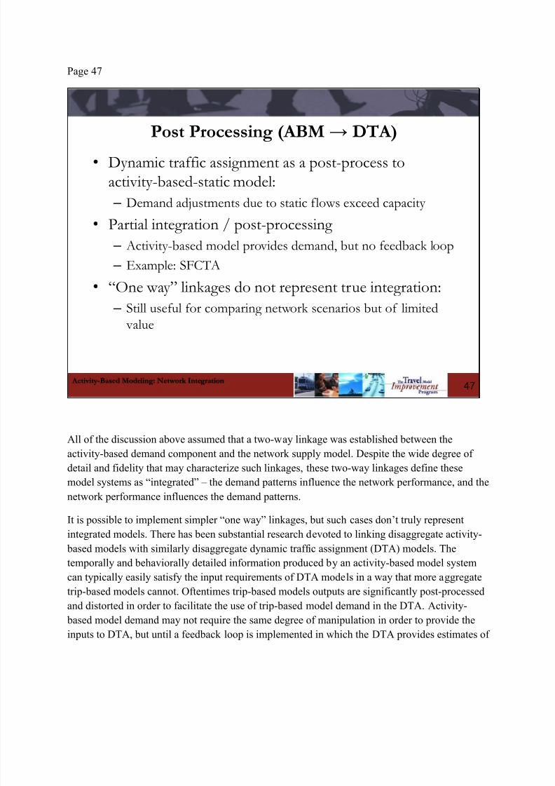
8/10/2019 Webinar11 Network Integration Slides-With-Notes2
http://slidepdf.com/reader/full/webinar11-network-integration-slides-with-notes2 64/102
Page 47
Activity-Based Modeling: Network Integration
Post Processing (ABM → DTA)• Dynamic traffic assignment as a post-process to
activity-based-static model:
– Demand adjustments due to static flows exceed capacity
• Partial integration / post-processing
– Activity-based model provides demand, but no feedback loop
– Example: SFCTA
• “One way” linkages do not represent true integration:
– Still useful for comparing network scenarios but of limited value
47
All of the discussion above assumed that a two-way linkage was established between the
activity-based demand component and the network supply model. Despite the wide degree of
detail and fidelity that may characterize such linkages, these two-way linkages define these
model systems as “integrated” – the demand patterns influence the network performance, and the
network performance influences the demand patterns.
It is possible to implement simpler “one way” linkages, but such cases don’t truly represent
integrated models. There has been substantial research devoted to linking disaggregate activity-
based models with similarly disaggregate dynamic traffic assignment (DTA) models. Thetemporally and behaviorally detailed information produced by an activity-based model system
can typically easily satisfy the input requirements of DTA models in a way that more aggregate
trip-based models cannot. Oftentimes trip-based models outputs are significantly post-processed
and distorted in order to facilitate the use of trip-based model demand in the DTA. Activity-
based model demand may not require the same degree of manipulation in order to provide the
inputs to DTA, but until a feedback loop is implemented in which the DTA provides estimates of

8/10/2019 Webinar11 Network Integration Slides-With-Notes2
http://slidepdf.com/reader/full/webinar11-network-integration-slides-with-notes2 65/102
network performance for input to the activity-based model, an integrated model has not been
established.
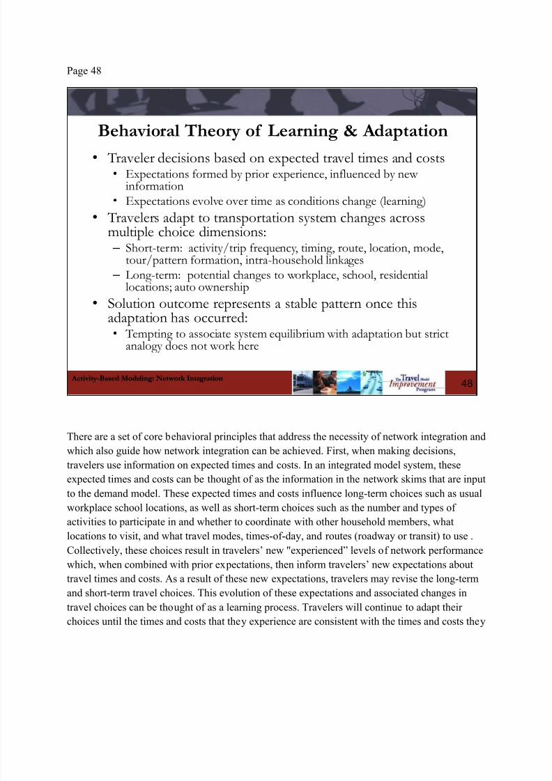
8/10/2019 Webinar11 Network Integration Slides-With-Notes2
http://slidepdf.com/reader/full/webinar11-network-integration-slides-with-notes2 66/102
Page 48
Activity-Based Modeling: Network Integration
Behavioral Theory of Learning & Adaptation• Traveler decisions based on expected travel times and costs
• Expectations formed by prior experience, influenced by newinformation
• Expectations evolve over time as conditions change (learning)
• Travelers adapt to transportation system changes acrossmultiple choice dimensions: – Short-term: activity/trip frequency, timing, route, location, mode,
tour/pattern formation, intra-household linkages
– Long-term: potential changes to workplace, school, residentiallocations; auto ownership
• Solution outcome represents a stable pattern once thisadaptation has occurred:• Tempting to associate system equilibrium with adaptation but strict
analogy does not work here
48
There are a set of core behavioral principles that address the necessity of network integration and
which also guide how network integration can be achieved. First, when making decisions,
travelers use information on expected times and costs. In an integrated model system, these
expected times and costs can be thought of as the information in the network skims that are input
to the demand model. These expected times and costs influence long-term choices such as usual
workplace school locations, as well as short-term choices such as the number and types of
activities to participate in and whether to coordinate with other household members, what
locations to visit, and what travel modes, times-of-day, and routes (roadway or transit) to use .
Collectively, these choices result in travelers’ new "experienced” levels of network performance
which, when combined with prior expectations, then inform travelers’ new expectations about
travel times and costs. As a result of these new expectations, travelers may revise the long-term
and short-term travel choices. This evolution of these expectations and associated changes in
travel choices can be thought of as a learning process. Travelers will continue to adapt their
choices until the times and costs that they experience are consistent with the times and costs they

8/10/2019 Webinar11 Network Integration Slides-With-Notes2
http://slidepdf.com/reader/full/webinar11-network-integration-slides-with-notes2 67/102
expected, at which point their choices will become stable. This overall iterative travel model
system may be considered an analog for this learning process.
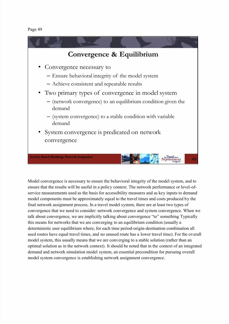
8/10/2019 Webinar11 Network Integration Slides-With-Notes2
http://slidepdf.com/reader/full/webinar11-network-integration-slides-with-notes2 68/102
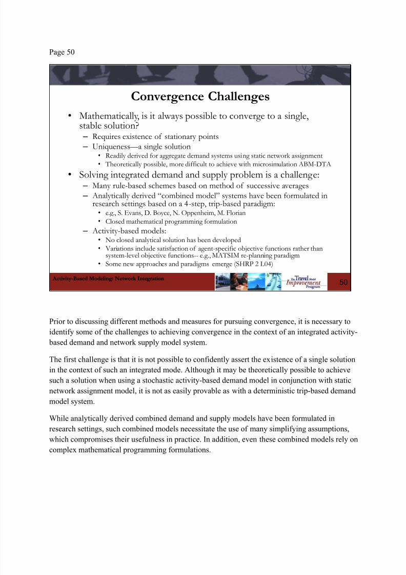
8/10/2019 Webinar11 Network Integration Slides-With-Notes2
http://slidepdf.com/reader/full/webinar11-network-integration-slides-with-notes2 69/102
Page 50
Activity-Based Modeling: Network Integration
Convergence Challenges• Mathematically, is it always possible to converge to a single,
stable solution? – Requires existence of stationary points
– Uniqueness — a single solution• Readily derived for aggregate demand systems using static network assignment• Theoretically possible, more difficult to achieve with microsimulation ABM-DTA
• Solving integrated demand and supply problem is a challenge: – Many rule-based schemes based on method of successive averages
– Analytically derived “combined model” systems have been formulated inresearch settings based on a 4-step, trip-based paradigm:
• e.g., S. Evans, D. Boyce, N. Oppenheim, M. Florian• Closed mathematical programming formulation
– Activity-based models:• No closed analytical solution has been developed• Variations include satisfaction of agent-specific objective functions rather than
system-level objective functions-- e.g., MATSIM re-planning paradigm• Some new approaches and paradigms emerge (SHRP 2 L04)
50
Prior to discussing different methods and measures for pursuing convergence, it is necessary to
identify some of the challenges to achieving convergence in the context of an integrated activity-
based demand and network supply model system.
The first challenge is that it is not possible to confidently assert the existence of a single solution
in the context of such an integrated mode. Although it may be theoretically possible to achieve
such a solution when using a stochastic activity-based demand model in conjunction with static
network assignment model, it is not as easily provable as with a deterministic trip-based demand
model system.
While analytically derived combined demand and supply models have been formulated in
research settings, such combined models necessitate the use of many simplifying assumptions,
which compromises their usefulness in practice. In addition, even these combined models rely on
complex mathematical programming formulations.

8/10/2019 Webinar11 Network Integration Slides-With-Notes2
http://slidepdf.com/reader/full/webinar11-network-integration-slides-with-notes2 70/102
In the context of activity-based models systems, no tractable analytical solution shave been
developed. Instead, both researchers and practitioners have primarily relied on heuristics such as
the method of successive averages in order to achieve stable results, although some agent-based
satisficing objective functions rather than system-level objective functions have been
successfully implemented.
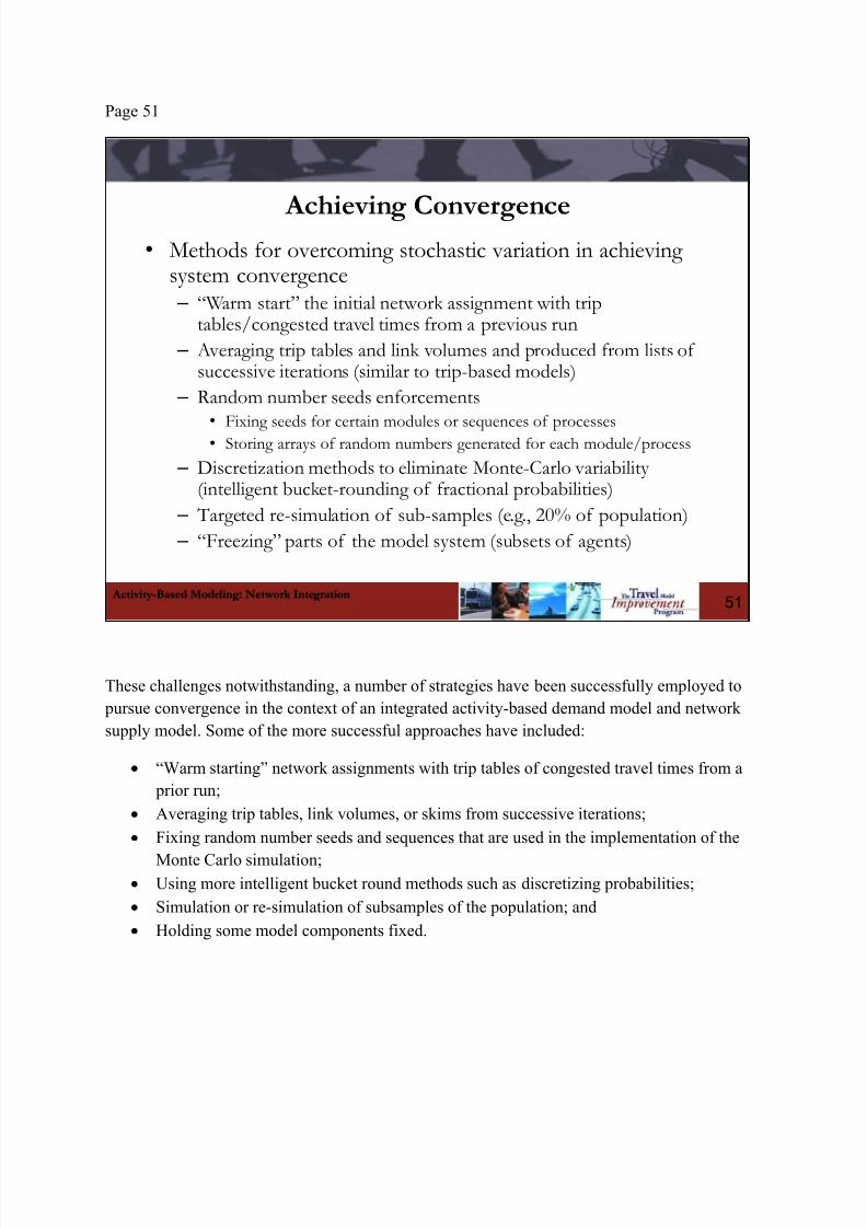
8/10/2019 Webinar11 Network Integration Slides-With-Notes2
http://slidepdf.com/reader/full/webinar11-network-integration-slides-with-notes2 71/102
Page 51
Activity-Based Modeling: Network Integration
Achieving Convergence• Methods for overcoming stochastic variation in achieving
system convergence – “Warm start” the initial network assignment with trip
tables/congested travel times from a previous run
– Averaging trip tables and link volumes and produced from lists ofsuccessive iterations (similar to trip-based models)
– Random number seeds enforcements•
Fixing seeds for certain modules or sequences of processes• Storing arrays of random numbers generated for each module/process
– Discretization methods to eliminate Monte-Carlo variability(intelligent bucket-rounding of fractional probabilities)
– Targeted re-simulation of sub-samples (e.g., 20% of population)
– “Freezing” parts of the model system (subsets of agents)
51
These challenges notwithstanding, a number of strategies have been successfully employed to
pursue convergence in the context of an integrated activity-based demand model and network
supply model. Some of the more successful approaches have included:
“Warm starting” network assignments with trip tables of congested travel times from a
prior run;
Averaging trip tables, link volumes, or skims from successive iterations;
Fixing random number seeds and sequences that are used in the implementation of the
Monte Carlo simulation; Using more intelligent bucket round methods such as discretizing probabilities;
Simulation or re-simulation of subsamples of the population; and
Holding some model components fixed.
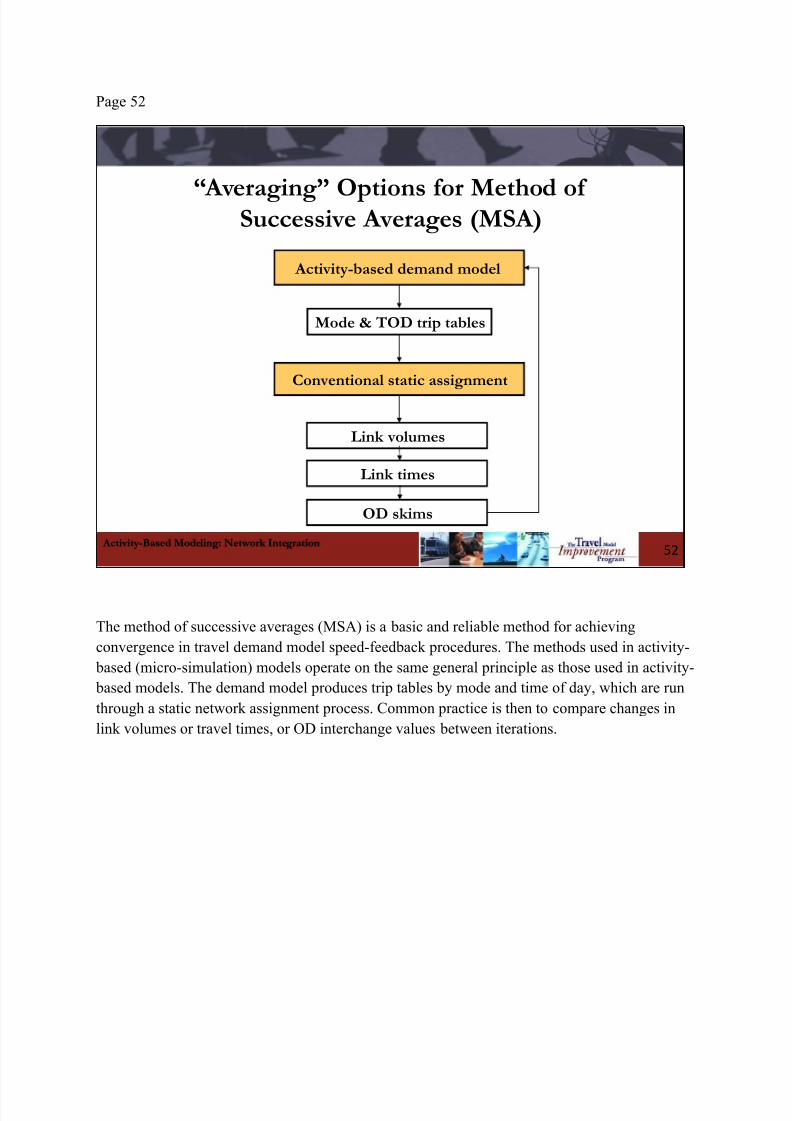
8/10/2019 Webinar11 Network Integration Slides-With-Notes2
http://slidepdf.com/reader/full/webinar11-network-integration-slides-with-notes2 72/102
Page 52
Activity-Based Modeling: Network Integration
“Averaging” Options for Method ofSuccessive Averages (MSA)
52
Activity-based demand model
Conventional static assignment
Mode & TOD trip tables
Link volumes
Link times
OD skims
The method of successive averages (MSA) is a basic and reliable method for achieving
convergence in travel demand model speed-feedback procedures. The methods used in activity-
based (micro-simulation) models operate on the same general principle as those used in activity-
based models. The demand model produces trip tables by mode and time of day, which are run
through a static network assignment process. Common practice is then to compare changes in
link volumes or travel times, or OD interchange values between iterations.
8/10/2019 Webinar11 Network Integration Slides-With-Notes2
http://slidepdf.com/reader/full/webinar11-network-integration-slides-with-notes2 73/102
Page 53
Activity-Based Modeling: Network Integration
Stopping Criteria• Based on either changes to link volumes and/or trip
tables… usually both
• Comparisons made for each relevant demand segment – E.g., SOV, HOV, Large trucks, Small/Medium trucks
• Link volume criteria example – Stop when 90% of link volumes change by less than 5%
– Often limited to higher-level facilities (e.g., freeways andarterials)
• Trip table criteria example – Stop when 80% of table cells change by less than 10%
– Often limited to minimum number of trips per cell (e.g., 100)
53
In addition to established methods for achieving convergence, it is also necessary to establish
measures for assessing model system convergence. Thus far, many of the convergence stopping
criteria used with integrated activity-based network supply models are similar to those used in
more traditional trip-based model systems. Many stopping criteria are based on looking at
changes in link volumes, or changes in trip table flows. The changes can be assessed in aggregate
across all demand segments, or may be considered for each segment independently. The specific
criterion can vary, but typically involves establishing that a significant share of link or cell
elements change less than an established threshold; for example, that 90% of link volumes
change by less than 5%. These criteria may also impose minimum size requirements, such as to
exclude all low volume links or low demand zone pairs.
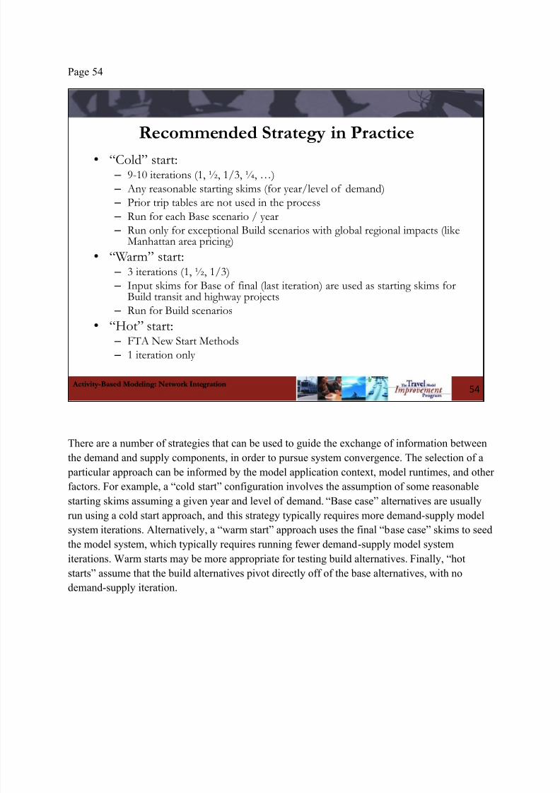
8/10/2019 Webinar11 Network Integration Slides-With-Notes2
http://slidepdf.com/reader/full/webinar11-network-integration-slides-with-notes2 74/102
Page 54
Activity-Based Modeling: Network Integration
Recommended Strategy in Practice• “Cold” start:
– 9-10 iterations (1, ½, 1/3, ¼, …)
– Any reasonable starting skims (for year/level of demand)
– Prior trip tables are not used in the process
– Run for each Base scenario / year – Run only for exceptional Build scenarios with global regional impacts (like
Manhattan area pricing)
• “Warm” start: –
3 iterations (1, ½, 1/3) – Input skims for Base of final (last iteration) are used as starting skims for
Build transit and highway projects
– Run for Build scenarios
• “Hot” start: – FTA New Start Methods
– 1 iteration only
54
There are a number of strategies that can be used to guide the exchange of information between
the demand and supply components, in order to pursue system convergence. The selection of a
particular approach can be informed by the model application context, model runtimes, and other
factors. For example, a “cold start” configuration involves the assumption of some reasonable
starting skims assuming a given year and level of demand. “Base case” alternatives are usually
run using a cold start approach, and this strategy typically requires more demand-supply model
system iterations. Alternatively, a “warm start” approach uses the final “base case” skims to seed
the model system, which typically requires running fewer demand-supply model system
iterations. Warm starts may be more appropriate for testing build alternatives. Finally, “hot
starts” assume that the build alternatives pivot directly off of the base alternatives, with no
demand-supply iteration.
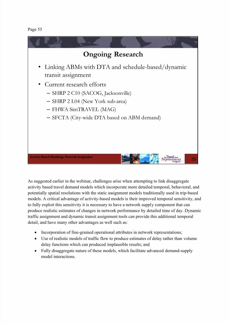
8/10/2019 Webinar11 Network Integration Slides-With-Notes2
http://slidepdf.com/reader/full/webinar11-network-integration-slides-with-notes2 75/102
Page 55
Activity-Based Modeling: Network Integration
Ongoing Research• Linking ABMs with DTA and schedule-based/dynamic
transit assignment
• Current research efforts
– SHRP 2 C10 (SACOG, Jacksonville)
– SHRP 2 L04 (New York sub-area)
– FHWA SimTRAVEL (MAG)
– SFCTA (City-wide DTA based on ABM demand)
55
As suggested earlier in the webinar, challenges arise when attempting to link disaggregate
activity based travel demand models which incorporate more detailed temporal, behavioral, and
potentially spatial resolutions with the static assignment models traditionally used in trip-based
models. A critical advantage of activity-based models is their improved temporal sensitivity, and
to fully exploit this sensitivity it is necessary to have a network supply component that can
produce realistic estimates of changes in network performance by detailed time of day. Dynamic
traffic assignment and dynamic transit assignment tools can provide this additional temporal
detail, and have many other advantages as well such as:
Incorporation of fine-grained operational attributes in network representations;
Use of realistic models of traffic flow to produce estimates of delay rather than volume
delay functions which can produced implausible results; and
Fully disaggregate nature of these models, which facilitate advanced demand-supply
model interactions.

8/10/2019 Webinar11 Network Integration Slides-With-Notes2
http://slidepdf.com/reader/full/webinar11-network-integration-slides-with-notes2 76/102

8/10/2019 Webinar11 Network Integration Slides-With-Notes2
http://slidepdf.com/reader/full/webinar11-network-integration-slides-with-notes2 77/102
Page 56
Activity-Based Modeling: Network Integration
Dynamic Traffic Assignment (DTA)• Advantages: capture time-varying network and demand
interactions in a more realistic way
• Sensitive to… – Time-varying demand
– Operational attributes (signal coordination, optimization,priorities)
–
Traffic dynamics (car following, queuing) – True capacity constraints
• Deployment scales – Project/corridor-level
– Regional-level (supports integration with regional demandmodel)
56
Dynamic traffic and transit assignment models are intended to provide more detailed means to
represent the interaction between travel choices, traffic flows, and time and cost measures in a
temporally consistent and behaviorally sound framework. More traditional static assignments
have a number of limitations, most critically their reliance of volume delay functions (VDFs).
Volume delay functions may be unreliable predictors of network performance because of their
dependence on volume/capacity ratios, which may counter-intuitively exceed 1.0, do not
incorporate critical operational attributes, do not reflect actual traffic phenomena such as
queuing, and do not reflect changes in impedances over time
In contrast, dynamic traffic assignment methods seek to explicitly represent the time-varying
nature of travel demand. This is achieved by implementing a number of fundamental departures
from static assignment methods, such as the incorporation of operational attributes which change
over time (for example, signal coordination) as well as the explicit representation of detail such
as the lane configurations. In addition, DTA models rely on traffic flow theory such as car
following and queuing to estimate delays, rather than using volume delay functions based on

8/10/2019 Webinar11 Network Integration Slides-With-Notes2
http://slidepdf.com/reader/full/webinar11-network-integration-slides-with-notes2 78/102
assumed capacities. This detailed modeling of traffic flows can provide better estimates of the
true capacity and performance of different facilities based on realistic operational constraints.
At present, DTA methods are increasingly used to support project-level analyses. However, such
applications typically represent “one way” linkages between the demand model and the DTA
model, and in fact demand model outputs are often extensively post-processed prior to use by theDTA model. The projects cited on the prior page represent some of cutting edge attempts to
deploy DTA approaches at a regional scale. Such a deployment is necessary in order to truly
provide useful information and integration with a regional activity-based model system.

8/10/2019 Webinar11 Network Integration Slides-With-Notes2
http://slidepdf.com/reader/full/webinar11-network-integration-slides-with-notes2 79/102
Page 57
Activity-Based Modeling: Network Integration
Dynamic Network Assignment Algorithms• Do away with V/C ratios — capacity constraints strictly
enforced through queuing and car following
• Intersection signal timing, lane geometries exert control
• Queuing behavior emerges
• Analytical solutions possible but difficult to implementdue to computational costs (memory and run-time)
• Heuristic solutions more practical, common in practice – Simulation of flows plus successive averaging
– Convergence not as “sure” as static assignment--difficult toachieve small relative gaps (2% considered “good”, 5%“acceptable”)
57
As described on the previous slides, DTA methods offer a number of compelling advantages
over traditional static assignment methodologies, such as more realistic representations of true
capacity constraints, operational attributes, and driver behavior. However, integration of DTA
models with regional activity-based demand models in order to achieve a fully disaggregate and
detailed travel demand models system is fraught with a number of challenges. Perhaps the most
significant challenge is that model system convergence is predicated on network supply model
convergence, but that network convergence using DTA methods is challenging. Although
analytic solutions are possible, they are extremely difficult to realize given the high computation
costs and runtimes. In practice, heuristic methods have proven to be more practical, but have not
been widely embraced by either the practitioner or research communities. And even the most
effective heuristic methods are unable to achieve levels of convergence that are easily achieved
using static methods. For example, convergence to a 2%-5% gap is typically considered good by
the DTA community, while convergence of 0.01% is usually easily achieved using static
methods.
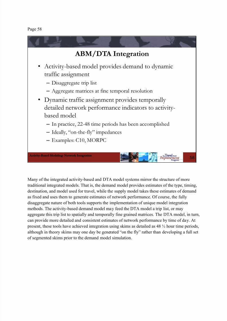
8/10/2019 Webinar11 Network Integration Slides-With-Notes2
http://slidepdf.com/reader/full/webinar11-network-integration-slides-with-notes2 80/102
Page 58
Activity-Based Modeling: Network Integration
ABM/DTA Integration• Activity-based model provides demand to dynamic
traffic assignment
– Disaggregate trip list
– Aggregate matrices at fine temporal resolution
• Dynamic traffic assignment provides temporallydetailed network performance indicators to activity-based model
– In practice, 22-48 time periods has been accomplished
– Ideally, “on-the-fly” impedances
– Examples: C10, MORPC
58
Many of the integrated activity-based and DTA model systems mirror the structure of more
traditional integrated models. That is, the demand model provides estimates of the type, timing,
destination, and model used for travel, while the supply model takes these estimates of demand
as fixed and uses them to generate estimates of network performance. Of course, the fully
disaggregate nature of both tools supports the implementation of unique model integration
methods. The activity-based demand model may feed the DTA model a trip list, or may
aggregate this trip list to spatially and temporally fine grained matrices. The DTA model, in turn,
can provide more detailed and consistent estimates of network performance by time of day. At
present, these tools have achieved integration using skims as detailed as 48 ½ hour time periods,
although in theory skims may one day be generated “on the fly” rather than developing a full set
of segmented skims prior to the demand model simulation.

8/10/2019 Webinar11 Network Integration Slides-With-Notes2
http://slidepdf.com/reader/full/webinar11-network-integration-slides-with-notes2 81/102
Page 59
Activity-Based Modeling: Network Integration
Conventional Integration Scheme
59
4-step demand model
Static assignment
Trip tables
LOS skims
for all
possible
trips
This is a reminder of the essence of conventional integration scheme in a 4-step model. Note that
trip tables and LOS skims are in exactly the same matrix format.
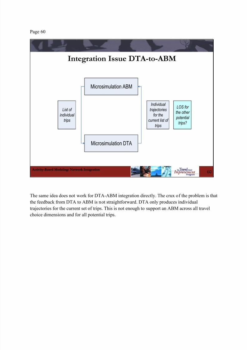
8/10/2019 Webinar11 Network Integration Slides-With-Notes2
http://slidepdf.com/reader/full/webinar11-network-integration-slides-with-notes2 82/102
Page 60
Activity-Based Modeling: Network Integration
Integration Issue DTA-to-ABM
60
Microsimulation ABM
Microsimulation DTA
List of
individual
trips
Individual
trajectories
for the
current list oftrips
LOS for
the other
potential
trips?
The same idea does not work for DTA-ABM integration directly. The crux of the problem is that
the feedback from DTA to ABM is not straightforward. DTA only produces individual
trajectories for the current set of trips. This is not enough to support an ABM across all travel
choice dimensions and for all potential trips.
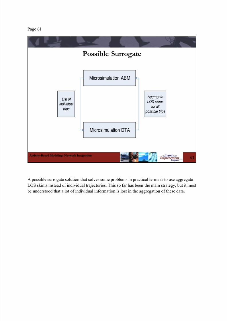
8/10/2019 Webinar11 Network Integration Slides-With-Notes2
http://slidepdf.com/reader/full/webinar11-network-integration-slides-with-notes2 83/102
Page 61
Activity-Based Modeling: Network Integration
Possible Surrogate
61
Microsimulation ABM
Microsimulation DTA
List of
individual
trips
Aggregate
LOS skims
for all
possible trips
A possible surrogate solution that solves some problems in practical terms is to use aggregate
LOS skims instead of individual trajectories. This so far has been the main strategy, but it must
be understood that a lot of individual information is lost in the aggregation of these data.
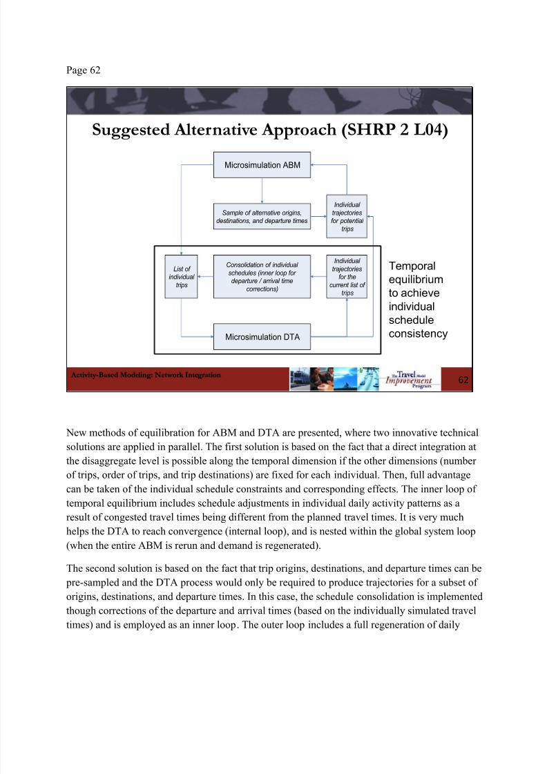
8/10/2019 Webinar11 Network Integration Slides-With-Notes2
http://slidepdf.com/reader/full/webinar11-network-integration-slides-with-notes2 84/102
Page 62
Activity-Based Modeling: Network Integration
Suggested Alternative Approach (SHRP 2 L04)
62
Microsimulation ABM
Microsimulation DTA
List ofindividual
trips
Individual
trajectoriesfor the
current list oftrips
Consolidation of individual
schedules (inner loop fordeparture / arrival time
corrections)
Sample of alternative origins,destinations, and departure times
Individual
trajectoriesfor potential
trips
Temporalequilibrium
to achieve
individual
schedule
consistency
New methods of equilibration for ABM and DTA are presented, where two innovative technical
solutions are applied in parallel. The first solution is based on the fact that a direct integration at
the disaggregate level is possible along the temporal dimension if the other dimensions (number
of trips, order of trips, and trip destinations) are fixed for each individual. Then, full advantage
can be taken of the individual schedule constraints and corresponding effects. The inner loop of
temporal equilibrium includes schedule adjustments in individual daily activity patterns as a
result of congested travel times being different from the planned travel times. It is very much
helps the DTA to reach convergence (internal loop), and is nested within the global system loop
(when the entire ABM is rerun and demand is regenerated).
The second solution is based on the fact that trip origins, destinations, and departure times can be
pre-sampled and the DTA process would only be required to produce trajectories for a subset of
origins, destinations, and departure times. In this case, the schedule consolidation is implemented
though corrections of the departure and arrival times (based on the individually simulated travel
times) and is employed as an inner loop. The outer loop includes a full regeneration of daily

8/10/2019 Webinar11 Network Integration Slides-With-Notes2
http://slidepdf.com/reader/full/webinar11-network-integration-slides-with-notes2 85/102
activity patterns and schedules but with a sub-sample of locations for which trajectories are
available.

8/10/2019 Webinar11 Network Integration Slides-With-Notes2
http://slidepdf.com/reader/full/webinar11-network-integration-slides-with-notes2 86/102
Page 63
Activity-Based Modeling: Network Integration
Individual Schedule Consistency
63
0 24
Activity i =0 Activity i =1 Activity i =2
Trip i =1 Trip i =2 Trip i =3
Activity i =3
Departure
Arrival
Duration
Travel
id
iT
i
i
Schedule
i
Individual schedule consistency means that for each person, the daily schedule (i.e., a sequence
of trips and activities) is formed without gaps or overlaps as shown on the slide. In this way, any
change in travel time would affect activity durations and vice versa.

8/10/2019 Webinar11 Network Integration Slides-With-Notes2
http://slidepdf.com/reader/full/webinar11-network-integration-slides-with-notes2 87/102
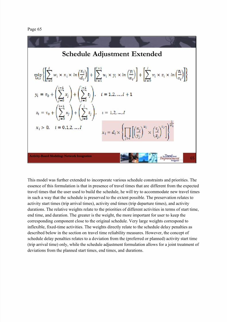
8/10/2019 Webinar11 Network Integration Slides-With-Notes2
http://slidepdf.com/reader/full/webinar11-network-integration-slides-with-notes2 88/102
Page 65
Activity-Based Modeling: Network Integration
Schedule Adjustment Extended
65
This model was further extended to incorporate various schedule constraints and priorities. The
essence of this formulation is that in presence of travel times that are different from the expected
travel times that the user used to build the schedule, he will try to accommodate new travel times
in such a way that the schedule is preserved to the extent possible. The preservation relates to
activity start times (trip arrival times), activity end times (trip departure times), and activity
durations. The relative weights relate to the priorities of different activities in terms of start time,
end time, and duration. The greater is the weight, the more important for user to keep the
corresponding component close to the original schedule. Very large weights correspond to
inflexible, fixed-time activities. The weights directly relate to the schedule delay penalties as
described below in the section on travel time reliability measures. However, the concept of
schedule delay penalties relates to a deviation from the (preferred or planned) activity start time
(trip arrival time) only, while the schedule adjustment formulation allows for a joint treatment of
deviations from the planned start times, end times, and durations.

8/10/2019 Webinar11 Network Integration Slides-With-Notes2
http://slidepdf.com/reader/full/webinar11-network-integration-slides-with-notes2 89/102
Page 66
Activity-Based Modeling: Network Integration
Weights for Schedule AdjustmentActivity type Duration Trip departure
(to activity)
Trip arrival (at
activity location)
Work (low income) 5 1 20
Work (high income) 5 1 5
School 20 1 20
Last trip to activity at home 1 1 3
Trip after work to NHB activity 1 5 1
Trip after work to NHB activity 1 10 1
NHB activity on at-work sub-tour 1 5 5
Medical 5 1 20
Escorting 1 1 20
Joint discretionary, visiting, eating out 5 5 10
Joint shopping 3 3 5
Any first activity of the day 1 5 1
Other activities 1 1 1
66
This is an example of typical weights applied in the schedule consolidation algorithm. These
weights can be further individualized. Note the extreme cases with high weights that correspond
to fixed schedule components. Lower weights correspond to flexible schedule components.

8/10/2019 Webinar11 Network Integration Slides-With-Notes2
http://slidepdf.com/reader/full/webinar11-network-integration-slides-with-notes2 90/102
Page 67
Activity-Based Modeling: Network Integration
Pre-Sampling of Trip Destinations• Primary destinations are pre-sampled:
– 300 out of 30,000 for each origin and travel segment,
– 30 out of 300 for each individual and travel segment
• Stop locations are pre-sampled: – 300 out of 30,000 for each OD pair and travel segment
– 30 out of 300 for each individual and travel segment
• Importance sampling w/o replacement from expandedset of destinations 300×30,000 and 30×300 to ensureuniform unbiased samples
• Efficient accumulation of individual trajectories inmicrosimulation process
67
This method is intended to resolve one of the fundamental problems associated with integration
of micro-simulation ABM and DTA – the calculation of individual LOS variables for non-
observed destinations and times of days (i.e. for trips that were not simulated at the previous
global iterations). It is also behaviorally more appealing to assume that an individual does not
always scan all possible location in the region for each activity but rather operate within a certain
spatial domain where he explores options over time and make choice based on the past
experience.

8/10/2019 Webinar11 Network Integration Slides-With-Notes2
http://slidepdf.com/reader/full/webinar11-network-integration-slides-with-notes2 91/102
Page 68
Activity-Based Modeling: Network Integration
LOS Skims for Outer Loop• (1st choice) Individual trajectories by departure time
period for the same driver (personal learningexperience), if not:
– (2nd choice) Individual trajectories by departure time periodacross individuals (what driver can hear from other people
through social networks), if not:
•
(3rd
choice) Aggregate OD skims by departure time period (advicefrom navigation device)
68
Pre-sampling of destination constrains the variation of destinations for each individual and
allows for an efficient accumulation of individual trajectories in the micro-simulation process.
With this technique, the LOS variables will be defined at each subsequent iteration as follows:
First, individual trajectories to the same destination by departure time period for the same
driver (or some other driver from the same household) are used if present in the previous
simulation; behaviorally, this corresponds to personal learning experience; having only
30 possible destinations enhances this probability for each individual; if not:
Individual trajectories to the same destination by departure time period across allindividuals are used if present in the previous simulation (if several of them are available,
the average can be used); behaviorally this corresponds to social networking when the
driver can hear from other people about their experience; having only 300 possible
destinations for each origin MAZ enhances this probability, if not:
Aggregate LOS skims by departure time period will be used as the last remaining option;
behaviorally it can be thought of as using an Advice from an advanced navigation device.

8/10/2019 Webinar11 Network Integration Slides-With-Notes2
http://slidepdf.com/reader/full/webinar11-network-integration-slides-with-notes2 92/102
Page 69
Activity-Based Modeling: Network Integration
Mode Choice Refinement for ABM-DTAIntegration: Driver vs. Passenger for HOV
Mode
Auto
SOV
Non-toll, GeneralPurpose lane
Toll, Managedlane
HOV2 driver, joint travel party
Non-toll, GeneralPurpose lane
Non-toll,Managed lane
Toll, Managedlane
HOV3+ driver, joint travel party
Non-toll, GeneralPurpose lane
Non-toll,Managed Lane
Toll, Managedlane
HOV2 passenger(not assigned)
Non-toll, GeneralPurpose lane
Non-toll,Managed lane
Toll, Managedlane
HOV3 passenger(not assigned)
Non-toll, GeneralPurpose lane
Non-toll,Managed lane
Toll, Managedlane
Transit
…
….
69
An advanced ABM incorporates intra-household carpools explicitly (joint travel by household
members is a separate travel segment) and inter-household carpools implicitly in the mode
choice process. This provides the necessary background for the refinement of mode choice that
should include both car occupancy and driver-passenger roles explicitly. In this way, the ABM
output in terms of person trips will be fully compatible with the DTA input required vehicle trips
by occupancy. Moreover, for more advanced integration schemes, the individual driver and
travel party characteristics including VOT and VOR can be carried over from the ABM to DTA.

8/10/2019 Webinar11 Network Integration Slides-With-Notes2
http://slidepdf.com/reader/full/webinar11-network-integration-slides-with-notes2 93/102
Page 70
Activity-Based Modeling: Network Integration
Trip Departure Time Choice Refinement (5 minresolution)• Tour TOD choice model:
– bi-directional and has 841 departure-arrival alternatives with30 min resolution
– Number of alternatives will quadruple with 15 min resolution
• Trip departure time choice model:
– One-directional
– 5 min resolution is feasible and results in under 100 ordered
alternatives
– Multiple Discrete-Continuous approach is being tested for
MAG ABM (ASU)
70
In order to make the ABM compatible with the temporal resolution of DTA, we suggest an
enhancement of the temporal resolution of the trip departure time choice model to 5 min. The
tour-level time-of-day choice model is characterized by a complicated two-dimensional choice of
outbound and inbound times that results in approximately 1,000 alternatives with 30-min
resolution. This choice dimension is difficult to further improve in terms of temporal resolution.
Also, in behavioral terms, there is no need in too much temporal detail in tour-level scheduling
anyway, since it does not yet have full information on the number/location of destinations visited
along the tour, so the exact timing and LOS information is only indicative at this point in the
simulation. However, trip-level choice of departure time that is conditional upon the entire-tour
time-of-day choice can be refined to 5 min, since the choice structure is one-dimensional and
more details about each particular trip origin and destination can be used.

8/10/2019 Webinar11 Network Integration Slides-With-Notes2
http://slidepdf.com/reader/full/webinar11-network-integration-slides-with-notes2 94/102
Page 71
Activity-Based Modeling: Network Integration
Integration - Continuous Exchange of Data• Linking an ABM with dynamic traffic and transit
assignment
• FHWA SimTRAVEL research project (Arizona State,U. Arizona, U.C. Berkeley)
• Assumes travelers have complete information and reactaccordingly in real time
• Would require fully integrated demand and supplymodels in a single program structure
71
One of the more ambitions research efforts currently underway is the FHWA sponsored
SimTravel project. This wide-ranging project is developing integrated models of the entire urban
system including location choices of households and firms, activity and travel patterns of
passengers and freight, and emergent traffic flows on time-dependent networks. Unlike
integrated models which seek to achieve an equilibrium condition by the repeated exchange of
demand and supply data, much of the early SimTravel work around demand and supply
integration is focused on “real time” interactions between the demand and supply components.
Ultimately, such an approach seems as though it may require fully integrated demand and supply
models in a single program structure. However, such an approach may also offer compelling
application and analysis capabilities.

8/10/2019 Webinar11 Network Integration Slides-With-Notes2
http://slidepdf.com/reader/full/webinar11-network-integration-slides-with-notes2 95/102
Page 72
Activity-Based Modeling: Network Integration
Schedule-based/Dynamic Transit Assignment• FHWA SimTRAVEL project
• Use actual/realistic transit schedules in conjunction withactivity-based models and dynamic traffic assignment – Drive access times affected by dynamic traffic assignment
– Bus transit operating in mixed traffic affected by surroundingtraffic stream
• Boarding and alighting times, crowding affect level of service
•Capacity constraints may result in bus bunching, travelers having to waitfor next bus
– Fixed guideway transit relatively simple if no-congestion effectmodeled
– Fixed guideway transit with capacity constraints affects boardingand alighting times
72
There have been several recent initial attempts to use actual/realistic transit schedules in
conjunction with activity-based models and dynamic traffic assignment. Specific efforts have
included attempts to model the following behavior:
Drive access times affected by dynamic traffic assignment;
Bus transit operating in mixed traffic affected by surrounding traffic stream;
Boarding and alighting times, crowding affect level of service;
Capacity constraints may result in bus bunching, travelers having to wait for another bus;
Fixed guideway transit relatively simple if no-congestion effect modeled; and Fixed guideway transit with capacity constraints affects boarding and alighting times.
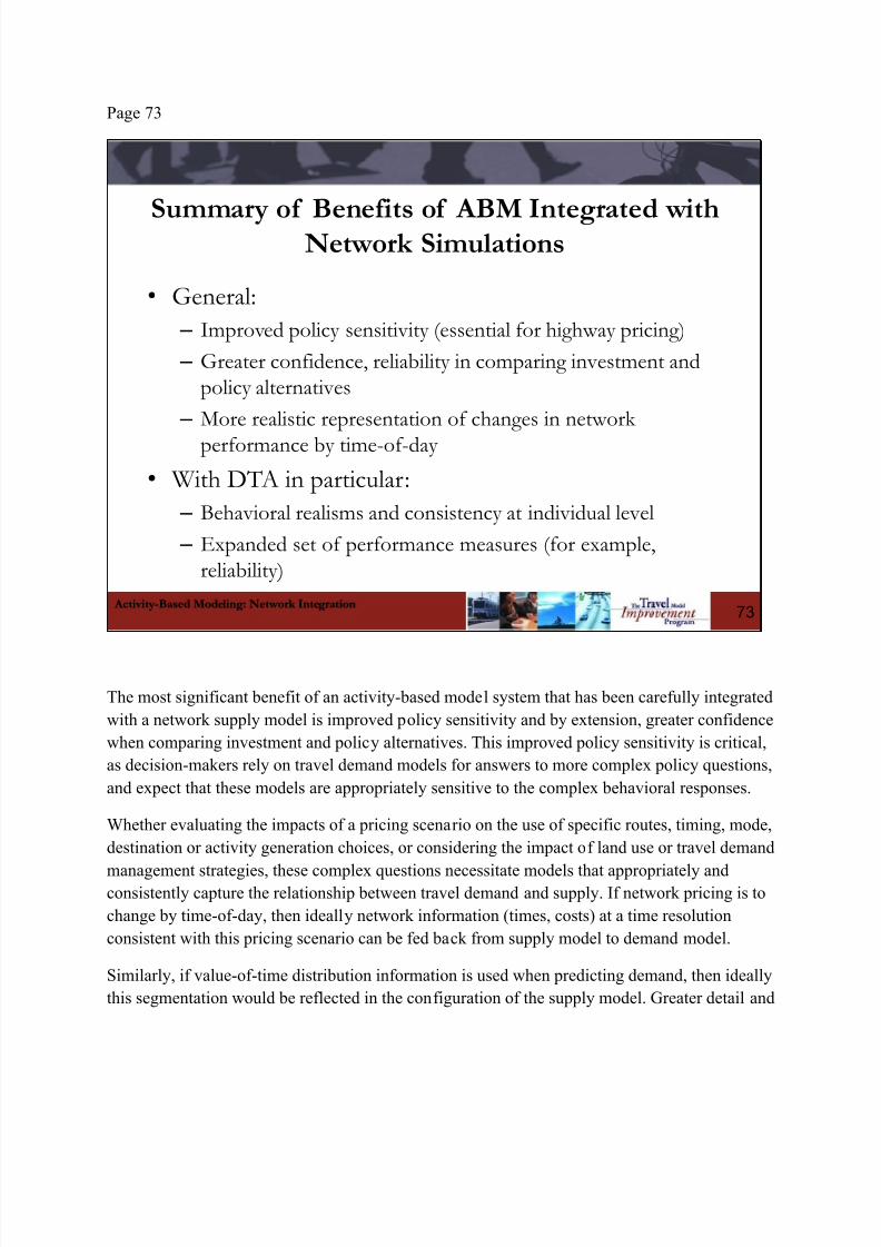
8/10/2019 Webinar11 Network Integration Slides-With-Notes2
http://slidepdf.com/reader/full/webinar11-network-integration-slides-with-notes2 96/102
Page 73
Activity-Based Modeling: Network Integration
Summary of Benefits of ABM Integrated withNetwork Simulations
• General:
– Improved policy sensitivity (essential for highway pricing)
– Greater confidence, reliability in comparing investment andpolicy alternatives
– More realistic representation of changes in network
performance by time-of-day
• With DTA in particular:
– Behavioral realisms and consistency at individual level
– Expanded set of performance measures (for example,reliability)
73
The most significant benefit of an activity-based model system that has been carefully integrated
with a network supply model is improved policy sensitivity and by extension, greater confidence
when comparing investment and policy alternatives. This improved policy sensitivity is critical,
as decision-makers rely on travel demand models for answers to more complex policy questions,
and expect that these models are appropriately sensitive to the complex behavioral responses.
Whether evaluating the impacts of a pricing scenario on the use of specific routes, timing, mode,
destination or activity generation choices, or considering the impact of land use or travel demand
management strategies, these complex questions necessitate models that appropriately andconsistently capture the relationship between travel demand and supply. If network pricing is to
change by time-of-day, then ideally network information (times, costs) at a time resolution
consistent with this pricing scenario can be fed back from supply model to demand model.
Similarly, if value-of-time distribution information is used when predicting demand, then ideally
this segmentation would be reflected in the configuration of the supply model. Greater detail and

8/10/2019 Webinar11 Network Integration Slides-With-Notes2
http://slidepdf.com/reader/full/webinar11-network-integration-slides-with-notes2 97/102
greater consistency between the demand and network supply components of the model system
lead to improved behavioral realism. In addition, this greater detail in both the demand and
supply components supports an expanded set of performance measures.

8/10/2019 Webinar11 Network Integration Slides-With-Notes2
http://slidepdf.com/reader/full/webinar11-network-integration-slides-with-notes2 98/102
Page 74
Activity-Based Modeling: Network Integration
Costs of Network Integrated ABM• Data and process development and maintenance:
– Network inputs
– Calibration / validation
• Runtime: – Stochastic variation may necessitate multiple demand
simulations
–
When ABM is integrated with static UE assignment, moredetail/resolution means longer runtimes• More time periods to assign
• More market segments to assign
– In DTA, no additional runtime costs due to demand detail,but assignment runtimes are extremely long to begin with
74
However, this improved policy sensitivity comes at a cost. From a data management perspective,
the development and maintenance of network inputs does require additional effort, and more
fine-grained calibration and validation efforts are also associated with this additional detail.
From a production standpoint, the additional time period and market segmentation results in
longer runtimes when using static assignment methods, although these runtimes differences
become less significant with improvements in network software and increases in hardware
computing power. Within the context of DTA, these runtime differences associated with
additional may detail become even less relevant. Depending on the specific application context,
stochastic variation associated with the use of the Monte Carlo simulation based activity model
may also necessitate multiple simulations and additional runtime, although the demand
components of most activity-based model systems typically account for only a small fraction of
total model runtimes.
8/10/2019 Webinar11 Network Integration Slides-With-Notes2
http://slidepdf.com/reader/full/webinar11-network-integration-slides-with-notes2 99/102
Page 75
Questions and Answers
75

8/10/2019 Webinar11 Network Integration Slides-With-Notes2
http://slidepdf.com/reader/full/webinar11-network-integration-slides-with-notes2 100/102
Page 76
Next Webinar
Executive and Management Sessions
Executive Perspective February 2
Institutional Topics for Managers February 23
Technical Issues for Managers March 15
Technical Sessions
Activity-Based Model Framework April 5
Population Synthesis and Household Evolution April 26
Accessibility and Treatment of Space May 17Long-Term and Medium Term Mobility Models June 7
Activity Pattern Generation June 28
Scheduling and Time of Day Choice July 19
Tour and Trip Mode, Intermediate Stop Location August 9
Network Integration August 30
Forecasting, Performance Measures and Software September 20
76

8/10/2019 Webinar11 Network Integration Slides-With-Notes2
http://slidepdf.com/reader/full/webinar11-network-integration-slides-with-notes2 101/102
Session 11 Questions and Answers
On slides 32 & 33 there was a depiction of a trip-based model with feedback and an activity-
based model and all of its components. Is it because we are working with travel behavior of
individuals in the synthetic population that the feedback can occur in any of these model steps?
Joe: No, I wouldn’t say it is because we are working with a synthetic population that all of this
feedback is possible. You could incorporate accessibility measures in a trip-based model, going
all the way back to auto ownership and trip generation. There are generally more components in
an activity-based model, and a conscious attempt to ensure upward and downward consistency
by incorporating feedback. But, it is not intrinsic to using a synthetic population. That being said,
by using individual agents, you can include more person-level and household-level attributes that
may be related to accessibility, so the structure does facilitate a more focused use of those
variables.
You mentioned some of the dangers of models that do not converge. Could you mention some
possible model simplifications to help an un-converging model find convergence?
Peter: There are methods to analyze the entire model system and identify trouble-makers. There
are specific components such as traffic assignment and mode choice for which we have very
good strategies for achieving convergence. What might be a problem is an attempt to make trip
generation or daily activity pattern, time of day, or destination choice over-sensitive, causing
oscillation and difficulty reaching convergence. The first important step is to diagnose which
model components are contributing to the lack of convergence, and there are diagnostic tests that
can be performed to identify the source. Secondly, one of the best ways to deal with non-convergence is to apply differential averaging strategies. Many people use a simple MSA
strategy or a naïve equilibration scale. These might need to be adjusted to achieve a better
convergence. Normally if you observe wild behavior, it’s likely that one of the model
components needs fixing before worrying about convergence.
Could one assume that demand and supply convergence go hand in hand? Are there
circumstances where one converges and the other does not?
Joe: It is dependent on the specific assignment method that is being used and the methods that
are used in the specific activity-based model. On the assignment side, if we are using a
traditional static-user-equilibrium method, and exposing the model to the same, converged
demand matrix, you should see convergence in the traffic assignment. As we get into advanced
network models such as dynamic traffic assignment, then it becomes more complicated, and it
might be found that you don’t see the same convergence. We might even need to reconsider how
we define convergence. Another issue is the Monte Carlo simulation in the demand models.
There are methods to hold the random seeds fixed, so that if you expose the activity-based model
to the same skims, you will see exactly the same trips. Then there issues in the specific issues in

8/10/2019 Webinar11 Network Integration Slides-With-Notes2
http://slidepdf.com/reader/full/webinar11-network-integration-slides-with-notes2 102/102
the way the models are interacted with each other. So, while you do expect the convergence to
go hand in hand, there are instances where it can’t be assumed, depending on the nature of the
implementation of the model.
This question concerns the potential of using DTA instead of static assignment, and what we do
if we are not using volume-to-capacity (V/C) ratios. Could V/C ratios be capped during staticassignment to better represent capacity constraints? If we are doing away with V/C ratios, what
criteria do we use to establish level of service?
Peter: This goes back to better understanding the differences between static assignment and
volume delay functions versus the simulation techniques such as car-following and queuing rules
in a dynamic assignment. There have been many publications showing that V/C ratios cannot
reliably establish travel time estimates, especially when V/C goes over one. This mechanism is
replaced by simulation in a DTA, and when volume approaches capacity, a variety of things
happen such as gridlock and queue spillback that more realistically address reality and do not
allow V/C to rise above one. The publications show that the DTA methods more accuratelyestimate travel times during congestion. Whenever you try to just cap V/C to get more accurate
travel times or stronger volume-delay functions, which we have tried to do, it doesn’t work. The
right way to go is have a tool such as DTA that actually represents the physical situation on the
road. We need a new approach, but I do understand the concern for simplified practical solutions.
While I don’t recommend capping V/C, you can scale time estimates from static assignment
based on observed values to provide a better matrix. But this is a temporary, surrogate solution,
and I think we need to take DTA seriously. This is the way to go.