week 1 review - university of oxfordpeople.maths.ox.ac.uk/griffit4/math_alive/1/stats...landon vs....
TRANSCRIPT

Naima Hammoud
Feb 14, 2017
Week 1 Review
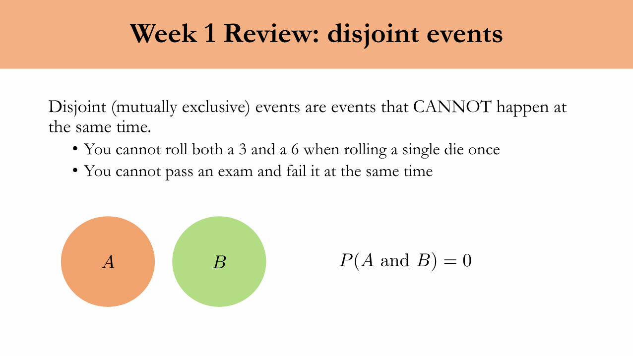
Disjoint (mutually exclusive) events are events that CANNOT happen at the same time.
• You cannot roll both a 3 and a 6 when rolling a single die once• You cannot pass an exam and fail it at the same time
A B P (A and B) = 0
Week 1 Review: disjoint events

Non-disjoint events are events that CAN happen at the same time.• You can pass a math exam and fail an English exam at the same time
A B
Week 1 Review: disjoint events
P (A and B) 6= 0

Probability of disjoint events:• Example: the probability of rolling a 3 OR a 6 on a single die roll
Probability of non-disjoint events:• Example: the probability of drawing a queen or a diamonds suit in a deck
of cards
Week 1 Review: disjoint events
P (3 or 6) = P (3) + P (6) =
1
6
+
1
6
=
1
3
Rolling 3
Rolling 6

P (Queen or diamond) = P (Queen) + P (diamond)� P (Queen and diamond)
=4
52+
13
52� 1
52⇡ 0.31

Week 1 Review: independence
Independent events: two events are independent if the outcome of the first event does not affect the outcome of the secondexample: if you toss a coin and get heads, you still have a 50% chance of getting heads on the second toss
Dependent events: Two events are dependent if the outcome of the first event affects the outcome of the secondexample: the probability of drawing a queen is 4/52. If you draw a queen, then the probability becomes 3/51.
P (A and B) = P (A)⇥ P (B)

Week 1 Review: conditional probability
Conditional Probability:
Bayes’ Theorem:
P (A|B) =P (A and B)
P (B)
P (A|B) =P (B|A)P (A)
P (B)

Week 1 Review: Basic Counting
26 26 26 10 10 10 10
Total number of choices = 26⇥ 26⇥ 26⇥ 10⇥ 10⇥ 10⇥ 10
If repetition is allowed

Week 1 Review: Basic Counting
If repetition is prohibited
26 25 24 10 9 8 7
Total number of choices = 26⇥ 25⇥ 24⇥ 10⇥ 9⇥ 8⇥ 7
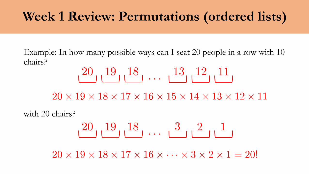
Week 1 Review: Permutations (ordered lists)
Example: In how many possible ways can I seat 20 people in a row with 10 chairs?
with 20 chairs?
. . .20 19 18 3 2 1
. . .20 19 18 13 12 11
20⇥ 19⇥ 18⇥ 17⇥ 16⇥ · · ·⇥ 3⇥ 2⇥ 1 = 20!
20⇥ 19⇥ 18⇥ 17⇥ 16⇥ 15⇥ 14⇥ 13⇥ 12⇥ 11

Week 1 Review: Combinations
How to choose k elements out of a total of n elements? (n and k are integers, with k less than or equal n)
Example: We toss a coin 10 times, in how many possible ways can we get 2 heads?
✓n
k
◆=
n!
k!(n� k)!0! = 1
✓10
2
◆=
10!
2!⇥ 8!=
10⇥ 9⇥ 8!
2⇥ 1⇥ 8!= 45
Naima Hammoud
Feb 14, 2017
Statistics: Part 1

What is it useful for?
• Surveys and polls: for example, we can conduct polls to see who people are voting for in the US presidential election. Then, using the data from the polls, we can make statements about who is more likely to win the election.
• Understanding the relation between two variables: for example, in a given neighborhood, how is the price of a house related to the number of rooms in the house?
• Inferring causal relations: for example, does cigarette smoking cause cancer?
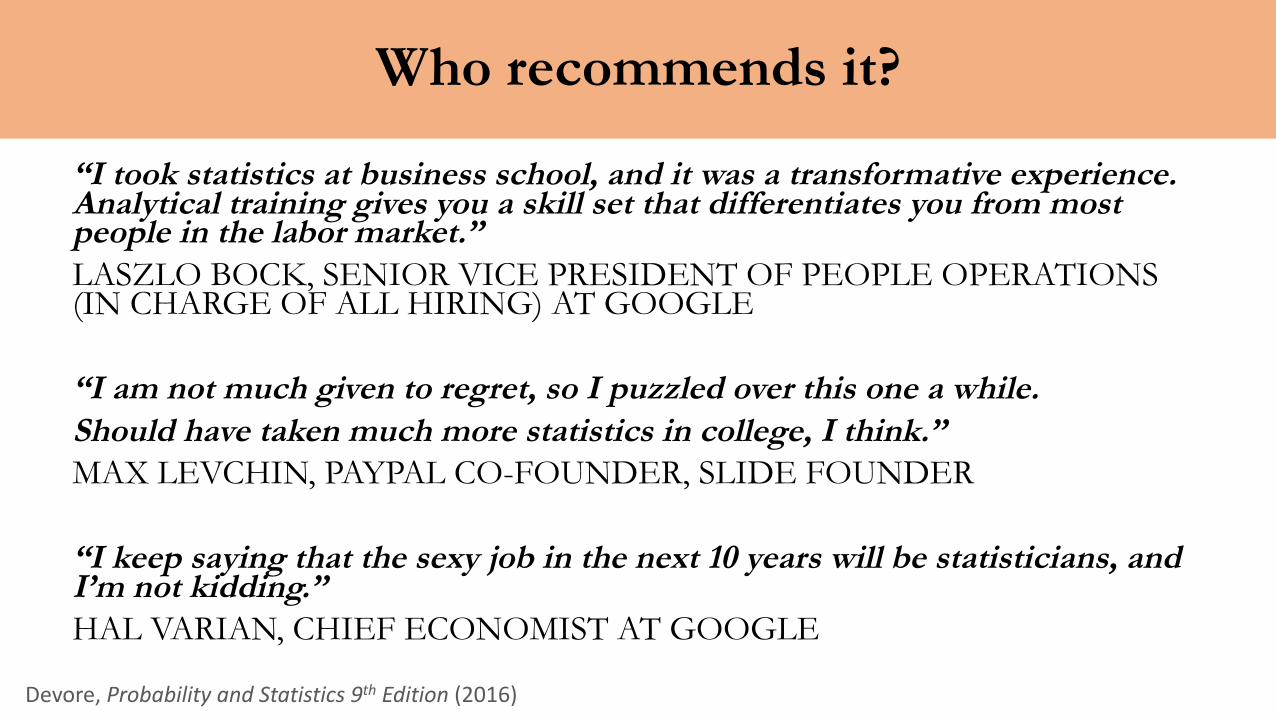
Who recommends it?
“I took statistics at business school, and it was a transformative experience. Analytical training gives you a skill set that differentiates you from most people in the labor market.” LASZLO BOCK, SENIOR VICE PRESIDENT OF PEOPLE OPERATIONS (IN CHARGE OF ALL HIRING) AT GOOGLE
“I am not much given to regret, so I puzzled over this one a while. Should have taken much more statistics in college, I think.” MAX LEVCHIN, PAYPAL CO-FOUNDER, SLIDE FOUNDER
“I keep saying that the sexy job in the next 10 years will be statisticians, and I’m not kidding.” HAL VARIAN, CHIEF ECONOMIST AT GOOGLE
Devore,ProbabilityandStatistics9th Edition(2016)

Introduction to Data
• Kinds of variables: numerical categorical
continuous discrete regular ordinal
Male Female
Very satisfiedSatisfiedNeutralDissatisfiedVery dissatisfied
Number of books you own
Your height

Correlation vs. Causation
observational study experiment
Want to study the effects of sleeping habits on energy levels
Study group of people who sleep and wake up at the same hour every day
Study a group of people who do do not have regular sleeping/waking up schedules
Randomly sample a group of people and assign them to sleep and wake up at the same hour every day
Randomly sample a group of people and assign them to sleep and wake up at different hours every day

Correlation vs. Causation
observational study experiment
Want to study the effects of sleeping habits on general health
wecanONLYestablishcorrelations

Correlation vs. Causation
observational study experiment
Want to study the effects of sleeping habits on general health
wecanONLYestablishcorrelations
wecanestablishcausalconnections
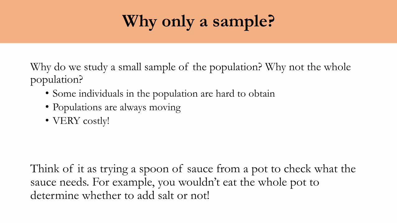
Why only a sample?
Why do we study a small sample of the population? Why not the whole population?
• Some individuals in the population are hard to obtain• Populations are always moving• VERY costly!
Think of it as trying a spoon of sauce from a pot to check what the sauce needs. For example, you wouldn’t eat the whole pot to determine whether to add salt or not!
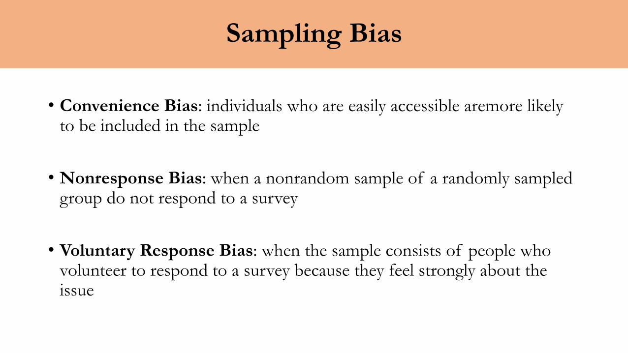
Sampling Bias
• Convenience Bias: individuals who are easily accessible aremore likely to be included in the sample
• Nonresponse Bias: when a nonrandom sample of a randomly sampled group do not respond to a survey
• Voluntary Response Bias: when the sample consists of people who volunteer to respond to a survey because they feel strongly about the issue

Sampling Bias: Historical ExamplesLandon vs. FDR
In 1936, the American Literary Digest magazine collected over two million surveys and predicted that the Republican nominee, Alf Landon, would beat Franklin Roosevelt 62% to 48%. The exact opposite happened!

Dewey vs. Truman
On election night in1948, the Chicago Tribune printed the headline
DEWEY DEFEATS TRUMAN
Survey was conducted via telephone

Data Visualization
Videofromwww.gapminder.com

Data visualization: Scatter Plot
This plot is useful when we want to study the relation between two variables. For example, life expectancy as a function of GDP per capita
Datasetfromwww.gapminder.comGDP per capita
lifeexpectancy
0
22.5
45
67.5
90
0 15000 30000 45000 60000

Data visualization: Histogram
Consider determining both the time to run the first 5 km and the time to run between the 35-km and 40-km points, and then subtracting the former time from the latter time.
Devore,ProbabilityandStatistics9th Edition(2016)

Skew
symmetric right skewedleft skewedno skew

Modality
unimodal
Devore,ProbabilityandStatistics9th Edition(2016)

Modality
multi-modal
Devore,ProbabilityandStatistics9th Edition(2016)

Modality
uniform
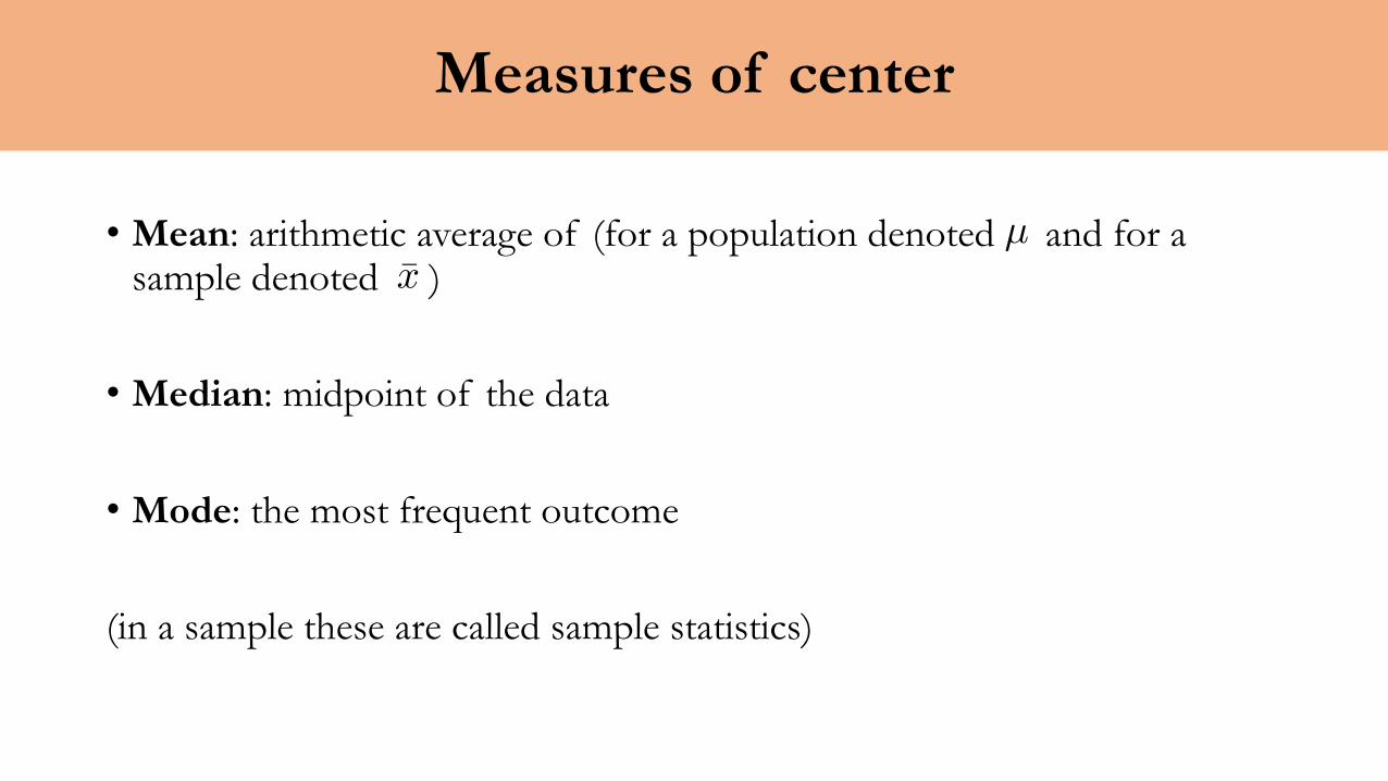
Measures of center
• Mean: arithmetic average of (for a population denoted and for a sample denoted )
• Median: midpoint of the data
• Mode: the most frequent outcome
(in a sample these are called sample statistics)
µx̄

Measures of center
9 scores on a homework (maximum score is 50): 38, 45, 35, 47, 42, 41, 50, 42, 39
mode : 42
median : 35, 38, 39, 41, 42, 42, 45, 47, 50
mean : x̄ =38 + 45 + 35 + 47 + 42 + 41 + 50 + 42 + 39
9= 42.1

Measures of center
10 scores on a homework (maximum score is 50): 35, 38, 39, 40, 41, 42, 42, 45, 47, 50
median =41 + 42
2= 41.5

Mean, median and skew
mean < median mean median⇡ mean > median

Measures of variability
• The easiest measure is the range: max – min (not a very useful measure)
• Variance: s2 for a population, s2 for a sample
• Standard deviation: s for a population, s for a sample
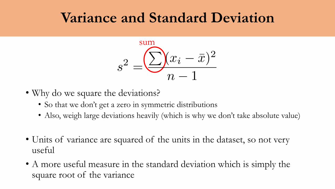
Variance and Standard Deviation
• Why do we square the deviations?• So that we don’t get a zero in symmetric distributions• Also, weigh large deviations heavily (which is why we don’t take absolute value)
• Units of variance are squared of the units in the dataset, so not very useful
• A more useful measure in the standard deviation which is simply the square root of the variance
sum
s
2 =
P(xi � x̄)2
n� 1

Example
The May 1, 2009, issue of The Montclarian reported the following home sale amounts for a sample of homes in Alameda, CA that were sold the previous month (1000s of $):
590, 815, 575, 608, 350, 1285, 408, 540, 555, 679
350, 408, 540, 555, 575, 590, 608, 679, 815, 1285
x̄ =590 + 815 + 575 + 608 + 350 + 1285 + 408 + 540 + 555 + 679
10= 640.5
Devore,ProbabilityandStatistics9th Edition(2016)median :
575 + 590
2= 582.5

Example
The May 1, 2009, issue of The Montclarian reported the following home sale amounts for a sample of homes in Alameda, CA that were sold the previous month (1000s of $):
590, 815, 575, 608, 350, 1285, 408, 540, 555, 679
So, a house in Alameda, CA costs on average thousand $
s2 =(590� 640.5)2 + (815� 640.5)2 + · · ·+ (555� 640.5)2 + (679� 640.5)2
9⇡ 67896
s =p67896 = 260.6
640.5± 260.6Devore,ProbabilityandStatistics9th Edition(2016)

Introduction to Inference
Case study on gender discrimination in 1972
48 bank supervisors (all male) were given the same personnel file and asked whether the person should be promoted or not. The files were identical, except that 24 of the files were assigned to belong to male employees, and 24 to females. Of the 48 files, 35 were promoted, 21 of which belonged to males, and the rest to females.
B.Rosen and T. Jerdee (1974), ``Influence of sex role stereotypes on personnel decisions", J.Applied Psychology

Data from case study
The percentage of men promoted is
The percentage of women promoted is
So there is a 30% difference between men and women promoted. Could this have been due to chance? Or, is there something going on?
21
24⇥ 100 = 88%
14
24⇥ 100 = 58%

Hypothesis Testing
• We will define a null hypothesis which says that nothing is going on, and this difference is merely due to chance
• Then we will introduce an alternative hypothesis which says that something is going on, that discrimination is actually happening, and that the difference could not have occurred due to chance
The null hypothesis is the status quo. We will stick to it unless we have evidence to favor the alternative hypothesis
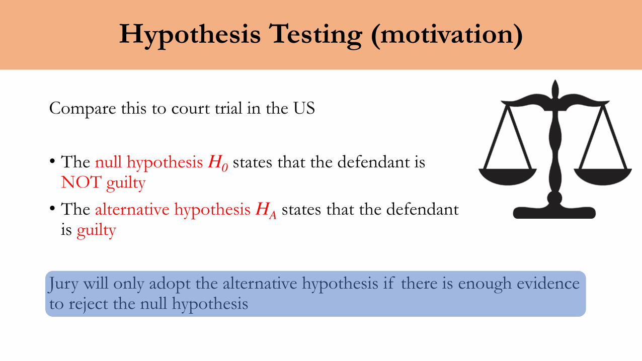
Hypothesis Testing (motivation)
Compare this to court trial in the US
• The null hypothesis H0 states that the defendant is NOT guilty
• The alternative hypothesis HA states that the defendant is guilty
Jury will only adopt the alternative hypothesis if there is enough evidence to reject the null hypothesis

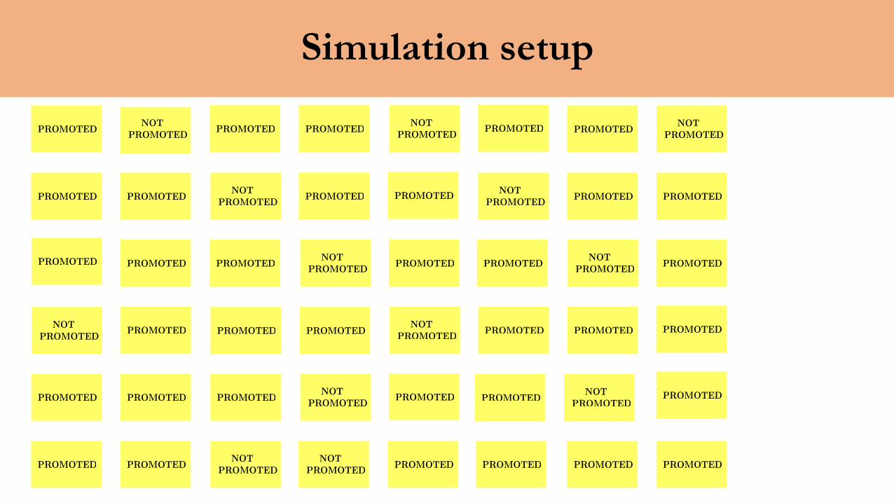
Simulation setup
We conduct 100 simulations using a computer, and we obtain the following results:
PROMOTEDNOT
PROMOTED
35 cards 13 cards

Simulation setup
PROMOTED PROMOTED PROMOTED PROMOTED PROMOTED PROMOTED PROMOTED PROMOTED
PROMOTED
PROMOTED
PROMOTED PROMOTED PROMOTED PROMOTED PROMOTED PROMOTED PROMOTED PROMOTED
PROMOTED PROMOTED
PROMOTED PROMOTED PROMOTED PROMOTED PROMOTED PROMOTED PROMOTED
PROMOTED PROMOTED PROMOTED
PROMOTED PROMOTED PROMOTED PROMOTED PROMOTED
NOTPROMOTED
NOTPROMOTED
NOTPROMOTED
NOTPROMOTED
NOTPROMOTED
NOTPROMOTED
NOTPROMOTED
NOTPROMOTED
NOTPROMOTED
NOTPROMOTED
NOTPROMOTED
NOTPROMOTED
NOTPROMOTED
Simulation setup
PROMOTEDNOT
PROMOTEDPROMOTED PROMOTED
NOTPROMOTED
NOTPROMOTED
PROMOTED PROMOTED PROMOTED PROMOTEDNOT
PROMOTED
PROMOTED PROMOTED
PROMOTED PROMOTED
NOTPROMOTED
NOTPROMOTED
PROMOTED PROMOTEDNOT
PROMOTEDPROMOTED PROMOTED
NOTPROMOTED
PROMOTEDPROMOTED
PROMOTED PROMOTED PROMOTEDNOT
PROMOTEDPROMOTED PROMOTED PROMOTED
PROMOTED PROMOTED PROMOTEDNOT
PROMOTEDPROMOTED PROMOTED
NOTPROMOTED
PROMOTED
NOTPROMOTED
PROMOTED PROMOTED PROMOTEDPROMOTEDNOT
PROMOTEDPROMOTED PROMOTED
women
men

Simulation setup
PROMOTEDNOT
PROMOTEDPROMOTED PROMOTED
NOTPROMOTED
NOTPROMOTED
PROMOTED PROMOTED PROMOTED PROMOTEDNOT
PROMOTED
PROMOTED PROMOTED
PROMOTED PROMOTED
NOTPROMOTED
NOTPROMOTED
PROMOTED PROMOTEDNOT
PROMOTEDPROMOTED PROMOTED
NOTPROMOTED
PROMOTEDPROMOTED
PROMOTED PROMOTED PROMOTEDNOT
PROMOTEDPROMOTED PROMOTED PROMOTED
PROMOTED PROMOTED PROMOTEDNOT
PROMOTEDPROMOTED PROMOTED
NOTPROMOTED
PROMOTED
NOTPROMOTED
PROMOTED PROMOTED PROMOTEDPROMOTEDNOT
PROMOTEDPROMOTED PROMOTED
men
women

Simulation setup
PROMOTEDNOT
PROMOTEDPROMOTED PROMOTED
NOTPROMOTED
NOTPROMOTED
PROMOTED PROMOTED PROMOTED PROMOTEDNOT
PROMOTED
PROMOTED PROMOTED
PROMOTED PROMOTED
NOTPROMOTED
NOTPROMOTED
PROMOTED PROMOTEDNOT
PROMOTEDPROMOTED PROMOTED
NOTPROMOTED
PROMOTEDPROMOTED
PROMOTED PROMOTED PROMOTEDNOT
PROMOTEDPROMOTED PROMOTED PROMOTED
PROMOTED PROMOTED PROMOTEDNOT
PROMOTEDPROMOTED PROMOTED
NOTPROMOTED
PROMOTED
NOTPROMOTED
PROMOTED PROMOTED PROMOTEDPROMOTEDNOT
PROMOTEDPROMOTED PROMOTED
women
men
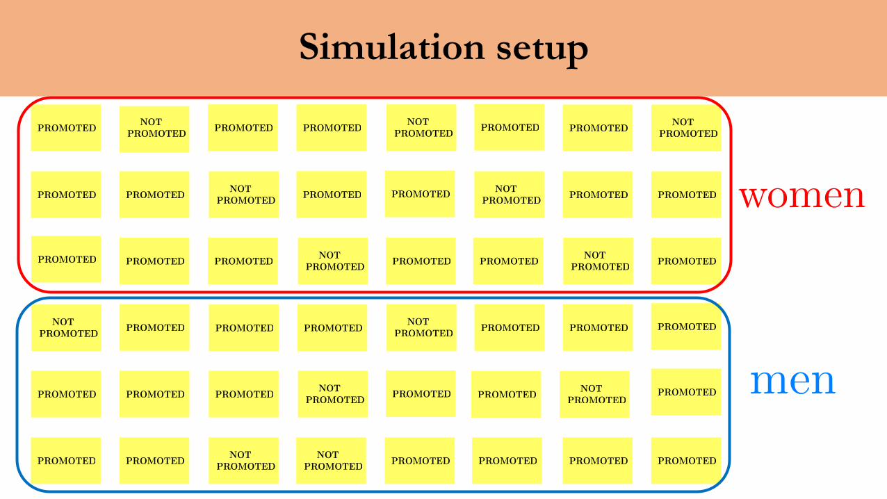
17 promoted

Simulation setup
PROMOTEDNOT
PROMOTEDPROMOTED PROMOTED
NOTPROMOTED
NOTPROMOTED
PROMOTED PROMOTED PROMOTED PROMOTEDNOT
PROMOTED
PROMOTED PROMOTED
PROMOTED PROMOTED
NOTPROMOTED
NOTPROMOTED
PROMOTED PROMOTEDNOT
PROMOTEDPROMOTED PROMOTED
NOTPROMOTED
PROMOTEDPROMOTED
PROMOTED PROMOTED PROMOTEDNOT
PROMOTEDPROMOTED PROMOTED PROMOTED
PROMOTED PROMOTED PROMOTEDNOT
PROMOTEDPROMOTED PROMOTED
NOTPROMOTED
PROMOTED
NOTPROMOTED
PROMOTED PROMOTED PROMOTEDPROMOTEDNOT
PROMOTEDPROMOTED PROMOTED
women
men
17 promoted

Simulation setup
PROMOTEDNOT
PROMOTEDPROMOTED PROMOTED
NOTPROMOTED
NOTPROMOTED
PROMOTED PROMOTED PROMOTED PROMOTEDNOT
PROMOTED
PROMOTED PROMOTED
PROMOTED PROMOTED
NOTPROMOTED
NOTPROMOTED
PROMOTED PROMOTEDNOT
PROMOTEDPROMOTED PROMOTED
NOTPROMOTED
PROMOTEDPROMOTED
PROMOTED PROMOTED PROMOTEDNOT
PROMOTEDPROMOTED PROMOTED PROMOTED
PROMOTED PROMOTED PROMOTEDNOT
PROMOTEDPROMOTED PROMOTED
NOTPROMOTED
PROMOTED
NOTPROMOTED
PROMOTED PROMOTED PROMOTEDPROMOTEDNOT
PROMOTEDPROMOTED PROMOTED
women
men18 promoted
17 promoted
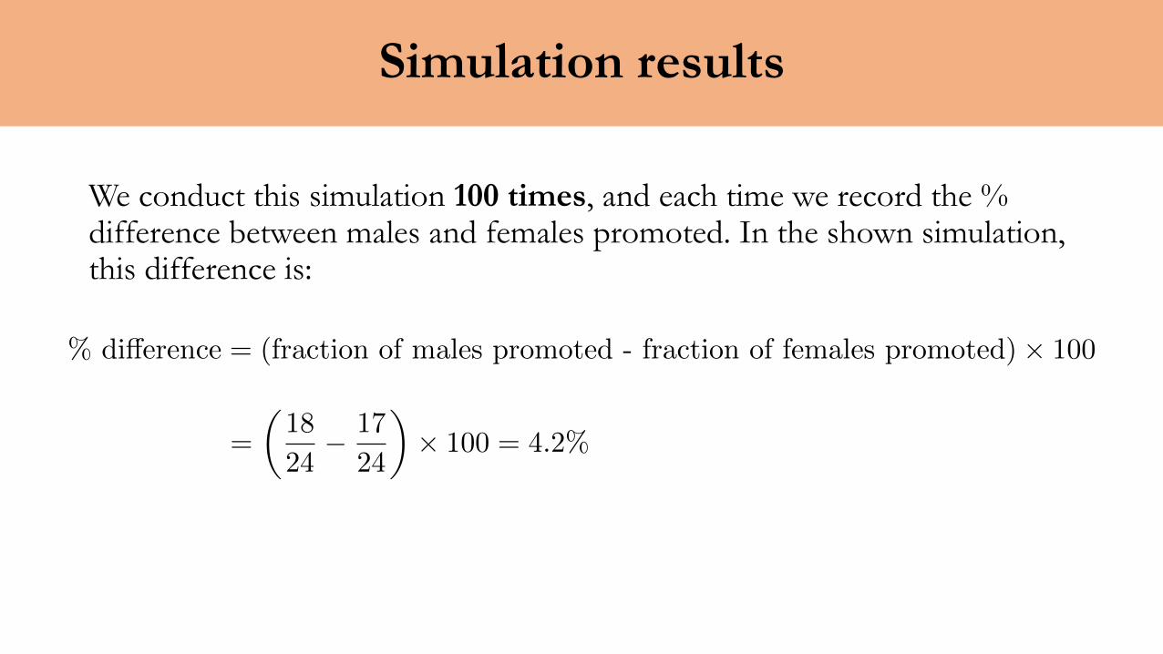
Simulation results
We conduct this simulation 100 times, and each time we record the % difference between males and females promoted. In the shown simulation, this difference is:
% di↵erence = (fraction of males promoted - fraction of females promoted)⇥ 100
=
✓18
24� 17
24
◆⇥ 100 = 4.2%

# of experiments Males promoted Femalespromoted
% difference inpromotion rates
1 13 22 -37.5%2 14 21 -29.2%6 15 20 -20.8%17 16 19 -12.5%25 17 18 -4.2%27 18 17 4.2%13 19 16 12.5%7 20 15 20.8%1 21 14 29.2%1 22 13 37.5%

Simulation results
percentage di↵erence in promotion rates
frequen
cy
0
7.5
15
22.5
30
-37.5% -29.2% -20.8% -12.5% -4.2% 4.2% 12.5% 20.8% 29.2% 37.5%
What is the probability to obtain a 30% or larger difference in promotion rates?
So there is a 1% chance that the results from the data are a matter of chance. What can we conclude?
1/100 = 0.01

Simulation conclusion
• If the test results do not provide convincing evidence for the alternative hypothesis, we stick with the null hypothesis.
• If there is enough evidence, we reject the null hypothesis in favor of the alternative hypothesis
Since there is only 1% chance the results could have occurred by chance, we can reject the null hypothesis in favor of the alternative hypothesis, and we conclude than indeed there is gender discrimination.

Hypothesis Testing Example
Amy has two roommates: Ryan and Hugo. Every week, Amy draws a name out of a bucket to randomly select which of the roommates is to take the trash out that week. Hugo suspects that Amy is cheating, so he starts keeping track of the draws, and he finds that out of 12 draws, Amy didn’t get picked even once!
Let’s perform a hypothesis testing that each of the roommates gets picked 1/3 of the time.
H0 : Amy is not cheating so each roommate gets picked 1/3 of the timeHA : Amy is cheating

Hypothesis Testing Example
H0 : Amy is not cheating so each roommate gets picked 1/3 of the timeHA : Amy is cheating
What is the probability that Amy doesn’t get picked a single time in 12 draws?
So there is a 0.7% chance that Amy doesn’t get picked 12 weeks in a row! Do you think this is by chance?
P (Amy not picked in 12 consecutive draws) =
P (Amy not picked in a given draw) =
2
3✓2
3
◆12
= 0.0077