NBER WORKING PAPER SERIES

WEEKENDS AND SUBJECTIVE WELL-BEING

John F. HelliwellShun Wang

Working Paper 17180http://www.nber.org/papers/w17180

NATIONAL BUREAU OF ECONOMIC RESEARCH1050 Massachusetts Avenue

Cambridge, MA 02138July 2011

This paper is part of the ‘Social Interactions, Identity and Well-Being’ research program of the CanadianInstitute for Advanced Research, and is also supported by grants from the Social Sciences and HumanitiesResearch Council of Canada. This support is gratefully acknowledged. We are grateful to the GallupCorporation for access to the Gallup/Healthways US daily poll. We thank Kevin Milligan and otherparticipants of the empirical lunch at the University of British Columbia for their comments. The viewsexpressed herein are those of the authors and do not necessarily reflect the views of the National Bureauof Economic Research.

NBER working papers are circulated for discussion and comment purposes. They have not been peer-reviewed or been subject to the review by the NBER Board of Directors that accompanies officialNBER publications.

© 2011 by John F. Helliwell and Shun Wang. All rights reserved. Short sections of text, not to exceedtwo paragraphs, may be quoted without explicit permission provided that full credit, including © notice,is given to the source.

Weekends and Subjective Well-BeingJohn F. Helliwell and Shun WangNBER Working Paper No. 17180July 2011JEL No. D69,J28,J81,Z19

ABSTRACT

This paper exploits the richness and large sample size of the Gallup/Healthways US daily poll to illustratesignificant differences in the dynamics of two key measures of subjective well-being: emotions andlife evaluations. We find that there is no day-of-week effect for life evaluations, represented here bythe Cantril Ladder, but significantly more happiness, enjoyment, and laughter, and significantly lessworry, sadness, and anger on weekends (including public holidays) than on weekdays. We then findstrong evidence of the importance of the social context, both at work and at home, in explaining thesize and likely determinants of the weekend effects for emotions. Weekend effects are twice as largefor full-time paid workers as for the rest of the population, and are much smaller for those whose worksupervisor is considered a partner rather than a boss and who report trustable and open work environments.A large portion of the weekend effects is explained by differences in the amount of time spent withfriends or family between weekends and weekdays (7.1 vs. 5.4 hours). The extra daily social timeof 1.7 hours in weekends raises average happiness by about 2%.

John F. HelliwellCanadian Institute for Advanced Researchand Department of EconomicsUniversity of British Columbia997-1873 East MallVancouver BC V6T 1Z1CANADAand NBERjohn.helliwell@ubc.ca

Shun WangDepartment of Economics,University of British Columbia997-1873 East MallVancouver B.C. V6T 1Z1 CANADAswangubc@hotmail.com

An online appendix is available at:http://www.nber.org/data-appendix/w17180

1

1. Introduction

Within and across nations, the search is on for better ways to measure how well

individuals, neighbourhoods, and societies are faring. Measures of subjective well-being

are at the centre of this search, and there are many initiatives to extend and improve local

and national accounts of subjective well-being. Central to the success of any such

ventures is the need to clarify what questions to ask, and to ensure that different measures

either tell the same or consistently different stories. An important distinction has been

made between life evaluations and reports of current emotions. One aspect of this is the

distinction between current and retrospective reports; a second is the contrast between

cognitive evaluations and emotional reports, and a third is related to long-running

philosophical discussions about the sources of good lives. Central to the latter is the

debate between those who emphasize the maximization of current pleasures (or the

excess of pleasures over pains) and those agreeing with the stoics that a good life is all

about doing the right thing. For those who adopt the epicurean, or more recently

Benthamite, view, the best measures of the quality of life would be given by summing

momentary evaluations, with as little retrospection as possible, of current pleasures and

pains. For those who follow a strong stoic position, the essence of a good life can be

assessed by the virtue it permits, and the capacities available to individuals. In this case,

subjective assessments of the quality of life are less important, or possibly even

misleading.

The middle ground on this issue is best exemplified by Aristotle, who argued that

neither the pleasure principle nor the stoic alternative was sufficient, and that a judicious

mix was required. He argued that the best way of seeing whether a good mix was

2

achieved would be to ask people to assess the quality of their lives. He hypothesized that

those who were most satisfied with their lives were those whose lives reflected doing

well for others as well as themselves, in ways that showed social engagement and a sense

of broader purpose.

Much of modern research on subjective well-being relies on some form of life

evaluation. The most common measure is the answer, often on a scale of zero to ten, of

how satisfied respondents are with their lives as a whole. Another, which is found in the

Gallup World Poll and in the Gallup/Healthways US daily poll data we use here, asks

respondents to think of their lives as a ladder, with the best possible life for them being

the top step, or a ten, and the worst possible as a zero. They are then asked to rate their

own current lives on this scale, and are sometimes also asked to assess in the same terms

their lives five years ago, and to forecast five years into the future. A third possibility has

been to ask people how happy they are with their lives as a whole. Some have argued that

both satisfaction and happiness are emotions, and that this will colour the answers given,

even if the focus is on life as a whole. It is to be expected that answers to questions about

a person’s state of happiness at the current moment, or yesterday, will vary from day to

day. If they do, how are the differences to be understood?

If answers to questions about positive and negative emotions are systematically

different from life evaluations, does that threaten the whole exercise? On the contrary, we

argue that the systematic differences increase the value and validity of both measures.

Both philosophy and psychology lead us to expect that the answers will differ in very

particular ways. If they do differ in the theoretically expected ways, then both types of

measure gain validity. The Gallup/Healthways US daily poll provides perhaps the best

3

data available to test some key hypotheses about the differences between current

emotions and life evaluations by seeing to what extent they vary according to temporary

circumstances. This is made possible by the size of the sample and frequency of

observations. The poll includes 1,000 observations each day on a wide range of variables

including a life evaluation (the Cantril Self-Anchoring Striving Scale, henceforth the

Cantril Ladder) and a range of questions asking about emotions felt during the previous

day. This focus on a particular day, combined with the large size of the sample, permits

the best chance of identifying day-of-week or weekend effects. Is there evidence to

support the storied ‘Blue Monday’ effect often appearing in song and stories, and studies

of the stock market (Pettengill 2003)? Are weekends happier or less happy, and why?

Rossi and Rossi (1977) show that positive emotions are more frequent on

weekends, but negative ones are not. Stone et al. (1985) find a significant weekend effect

rather than “Blue Monday” effect for moods. Egloff et al. (1995) find that pleasantness

peaks on weekends in a survey of college students. Kennedy-Moore et al. (1992) find that

both positive and negative affect show weekend effects. Csikszentmihalyi and Hunter

(2003) find that happiness peaks on weekends based on a survey for US school students

in the 6th, 8th, 10th and 12th grades. Most of these results, although they give relatively

consistent findings of weekend effects for emotions, have limited statistical power

because of their small sample sizes. There has been much less study of day-of-week

effects for life evaluations. The only one we located is Akay and Martinsson (2009) who

find a very small negative life satisfaction effect for Sunday using the German Socio-

Economic Panel data. The studies listed above are not able to compare weekend effects

for emotions with those for life evaluations. By using the Gallup/Healthways US daily

4

poll, we are able to harness the statistical power of sample sizes including more than half

a million respondents, randomly assigned by day of week, and containing answers for

one life evaluation and six emotions, of which three are positive and three negative.

Our first hypothesis is that if there are systematic day-of-week effects for emotions,

they will show up in the Gallup/Healthways daily data. Furthermore, and more

fundamentally, if there are significant day-of-week effects for emotions, they will be

smaller or absent for life evaluations, which we think to be more heavily dependent on

the overall circumstances of life. The latter part of the hypothesis has already been

shown: life evaluations are much more significantly determined by social and economic

life circumstances than are emotions. But now we are able to make a strong test of the

first part of the hypothesis: that short-term conditions of life will affect current emotions

much more than they affect life evaluations.

We find that US respondents are significantly happier, have more enjoyment, and

laugh more, while feeling less worry, sadness, and anger, on weekends (including public

holidays) than on weekdays. By contrast, there is no evidence supporting day-of-week

effects for the Cantril Ladder. The size of the weekend effects for emotions is seen to

depend on variables reflecting some aspects of the relative attractiveness of life at home

and at work.

When we turn to explain the size and potential determinants of weekend effects,

previous studies provide some clues. Kennedy-Moore et al. (1992) show that the greater

relative frequency of desirable events, and the reverse for undesirable ones, on weekends

compared to weekdays can partially explain the weekend effects. Csikszentmihalyi and

Hunter (2003) show that students spending more time in school and in social activities

5

are happier than those who spend less. We hypothesize that the size of weekend effects

for emotions is determined primarily by the extent and quality of the respondent’s social

connections on the weekend compared to those during the week. Our analysis shows that

most of the weekend effects is due to the greater time respondents are able to spend in

valued social interactions with friends or family. While social time is at least as valuable

to them on weekdays as it is on weekends, the additional 1.7 hours per day they spend in

the company of friends or family during the weekend explains a large part of the

weekend effects, especially for positive emotions.

In concluding, we will argue that our research shows the importance of measuring

both life evaluations and emotions, and the need to do so in comparable ways in the same

surveys. It will also be important to see if and to what extent our findings carry over to

other countries. The weekend effects show that working life has emotional costs for

typical US respondents, and yet the United States has the longest working hours among

all comparable countries. Are weekend effects smaller in countries with shorter working

hours and weeks? Or is there too much else in play by way of international differences in

intra-week variations in emotions? Is the social context of well-being equally important

in other countries, and are the resulting impacts on weekend happiness replicated in other

countries?

The rest of the paper is organized as follows. Section 2 describes the data. Section 3

presents the day-of-week effects for life evaluations and emotions. Section 4 explores the

likely sources of the weekend effects by sub-group analysis and Oaxaca (1973)-Blinder

(1973) decomposition. Section 5 concludes.

6

2. Data

This study uses data from the Gallup/Healthways US daily poll. Currently we have

the data from January 2, 2008 to June 30, 2009. The survey method for the poll relies on

live interviewers conducting telephone interviews with randomly sampled respondents

aged 18 and older, including cell phone users and Spanish-speaking respondents from all

50 states and the District of Columbia. It covers around 1,000 survey respondents each

day, and 527,281 respondents in total.

The poll contains answers for one life evaluation and six emotions. The life

evaluation measure used in the poll is the Cantril Ladder, a zero to ten scale response to

the question “On which step of the ladder would you say you personally feel you stand at

this time?” There are three positive emotions including happiness, enjoyment, and

laughter, and three negative ones including worry, sadness, and anger. The emotions are

zero to one scale responses to the question “Did you experience the following feelings

during a lot of the day yesterday?” Laughter is a zero to one scale response to the

question “Did you smile or laugh a lot yesterday?”

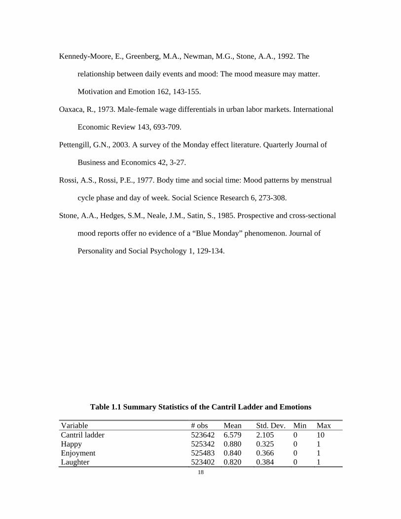
Table 1.1 presents summary statistics for the Cantril Ladder and emotions. The

average Cantril Ladder score is 6.6. The proportions of respondents reporting positive

emotions are much higher than those reporting negative emotions. Specifically, the

average values for happiness, enjoyment, and laughter are 88.0%, 84.0%, and 82.0%,

while those for worry, sadness, and anger are 32.3%, 18.1%, and 14.0%, respectively.

The survey includes many socio-demographic variables, including gender, age,

marital status, number of children under 18, education, employment status, monthly

household income, importance of religion in life, and social time spent with friends and

7

families. The monthly household income means the before-tax income including income

from wages and salaries, remittances from family members living elsewhere, farming,

and all other sources. The original response to the income question is on a zero to ten

scale, in which zero to ten stands for no income, under $60, $60 to $499, $500 to $999,

$1,000 to $1,999, $2,000 to $2,999, $3,000 to $3,999, $4,000 to $4,999, $5,000 to $7,499,

$7,500 to $9,999, and $10,000 and over, respectively. We then replace the categorical

response by the mean of each corresponding category to construct a numerical income

variable. The social hours variable is a response to the question “Approximately, how

many hours did you spend, socially, with friends or family yesterday? Please include

telephone or e-mail or other online communication.” The answer to this question ranges

between 0 and 24. About 5% of respondents report more than 16 social hours. To make

this social hours variable more reliable, we recode the values between 16 and 24 as 16.

The survey contains also two workplace environment questions and one job satisfaction

question for those in the working population. One is “Does your supervisor at work treat

you more like he or she is your boss or your partner?” Another is “Does your supervisor

always create an environment that is trusting and open, or not?” The job satisfaction

question is “Are you satisfied or dissatisfied with your job or the work you do?” Table

1.2 presents summary statistics for those variables.

3. Blue Monday or blue all week?

In this section, we explore the day-of-week distributions for the Cantril ladder and

emotions. Table 2 reports the estimated means and standard errors for the Cantil Ladder

and each emotion on each day of week and public holidays. Figure 1 illustrates the mean

8

difference of emotion between on Monday and on other weekdays. If Blue Monday

represented the worst day, then positive emotions would be better and negative emotions

worse than on all of the other days. What do the data show? The data show that there

simply are no day-of-week differences for life evaluations, as represented by the Cantril

Ladder. This adds to the growing weight of evidence that these are cognitive evaluations

principally driven by differences in life circumstances. For all of the daily emotional

reports, there is a significant daily pattern, with emotions being roughly equal every

weekday and significantly better on the weekends and public holidays.

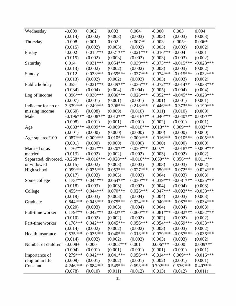
We then conduct OLS regressions for the day-of-week effects for the Cantril

Ladder and the six emotion measures, happiness, enjoyment, laughter, worry, sadness,

and anger, controlling for socio-demographic variables as well as public holidays, month,

year, and state dummies. The results are reported in Table 3 and illustrated in Figure 2.

Overall, the regression results show no day-of-week differences for the Cantril Ladder,

but a very distinctive pattern for emotions with the two weekend days and public holidays

differing from regular weekdays. The holiday effect is not significantly different from the

weekend effect at 5% significant level for each emotion. Thus all of our subsequent

analysis is simplified by the ease with which the daily effects can be compressed into a

weekend effect, where public holidays are treated as weekend days. This permits a much

clearer analysis of their patterns and likely causes. We now proceed to our analysis of the

weekend effects for emotions, having established at the outset the primary result that the

day-of-week effects are strongly present in emotions and absent for life evaluations.

9

4. Sources of weekend effects

In this section we explore the likely sources of weekend effects for emotions. We

first show that the survey date of reporting emotions ‘yesterday’ does not have significant

effect on the emotions. Intuitively respondents surveyed on the eve of or during a public

holiday might show higher positive emotions and lower negative emotions. To examine

whether there exist such effects, we compare the emotions on those weekdays

(specifically Monday to Thursday) followed by public holidays with those not followed

by public holidays by regressing each of the six emotions by a dummy variable equal to

one for those weekdays followed by public holidays and zero otherwise. As shown in

Table 4, there is no significant difference in happiness, worry, sadness, and angry

between the two categories of weekdays but even lower enjoyment and laughter on the

weekdays followed by public holidays. This result supports the conjecture that the report

of emotions is not significantly driven by expectation of impending holidays or by date of

reporting. We next conduct a series of sub-group analyses and Blinder-Oaxaca

decomposition to explore the potential driving forces of weekend effects.

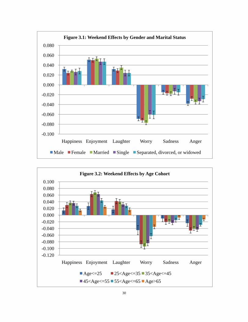
4.1 Weekend patterns by gender, family structure and age

Tables 5.1 and 5.2, and Figures 3.1 and 3.2, provide demographic decompositions

of the weekend effects. These weekend effects are estimated separately for each of the

demographic groups in question. Naturally, all of these demographic variables are also

correlated with other variables with important links to the weekend effect, such as health

and employment status. We shall later use more complete modeling to tease out the

10

separate impacts of a range of contributing factors. But these preliminary results expose

in a useful way some of the patterns to be explained.

We start with Figure 3.1 showing the weekend effects by gender and marital status.

Weekend effects for happiness and anger are significantly larger for males than females,

while for other emotions the gender differences are not significant. Indeed, the average

happiness advantage favouring females is entirely due to the fact that there are more

weekdays than weekends, as males are slightly happier than females on weekends, with

the reverse being true on weekdays. This is consistent with other evidence finding that

women value high trust (and hence happier) workplaces more than men, and are more

likely to find and stay in such jobs (Helliwell and Huang 2010, figures 5 and 6).

For all emotions weekend effects are bigger for the married than for others, and

significantly so for happiness, laughter, and worry. This is probably another sign of the

importance of the social context, as the weekend provides more time for those in well-

functioning family units to have time together. Our later results also show that having

children has a more positive effect on emotions during the weekend than on weekdays,

suggesting that weekends permit more relaxed, or at least less harried, family times. To

some extent this will be revealed by our social hours variables, but the effect apparently

extends further than that, as there is some evidence of it even after weekend social hours

are taken into account. The fact that positive emotions are more frequent, and negative

emotions less prevalent, on the weekends for the married implies that on average family

relations are friendly rather than the reverse.

Figure 3.2 shows a striking age pattern. To a significant extent, the established age

patterns in subjective well-being, whereby life evaluations and positive emotions follow a

11

U-shape with a low point about age 50, is diminished during the weekends. This is

consistent with previous findings that the U-shape was more pronounced, and the mid-

life low-point lower, for those who felt themselves unable to achieve work/life balance.

Since weekends are on average a time when work pressures fade into the background,

then we should expect the U-shape to be less then, especially for full-time workers. The

weekend offsets but does not eliminate the U-shape: we show later that it is about one-

quarter smaller on weekends than on weekdays.

4.2 The importance of trust and the social context at work

From the gender effects in Figure 3.1, we were starting to see hints that the social

context at work might have something to do with the size of weekend effects. Where

workmates are friends and the job is a pleasure, the weekend should make less difference,

since one is simply changing one set of friends for another. However, if the climate of

workplace trust is poisonous, and the job unsatisfying, then we should expect to find

significantly more positive emotions and fewer negative emotions during weekends.

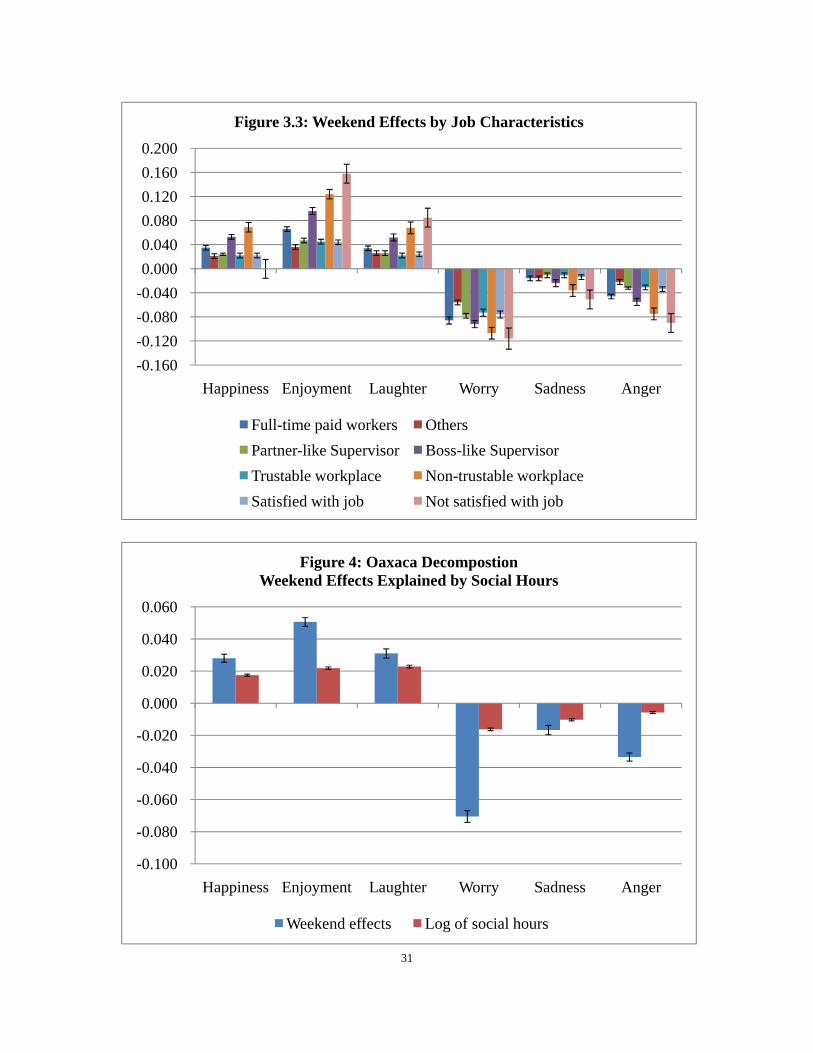
Table 5.3 and Figure 3.3 show four different ways of separating the size of

weekend effects according to job characteristics. First we show that weekdays are a lot

less fun than the weekends for those in full-time employment. The weekend effect is

about twice as large for the full-time employed as for the rest of the population. This does

not mean that people are not happy to have jobs. Our equations show, on the contrary,

that full-time workers are on average happier. What we are showing here is that a

substantial part of this extra happiness shows up during their well-earned weekends. This

12

is consistent with the additional result that part-time workers have weekend effects that

do not differ significantly from those for the non-working population.

Second, the Gallup/Healthways US daily poll asks a substantial fraction of

employed workers whether they consider their immediate work supervisor as a partner

rather than a boss. Figure 3.3 shows that weekend effects are significantly smaller, less

than half as large in the case of happiness, enjoyment, laughter, and sadness, for those

whose supervisors are viewed as partners rather than bosses. Third, we split the employed

samples based on whether the workplace environment is trusting and open. Figure 3.3

shows that weekend effects are approximately two times larger in the case of happiness,

enjoyment, laughter and sadness, one and a half larger in the case of anger, as well as one

half larger in the case of worry, for those who are in low-trust workplaces. The better the

social context of the job, the smaller differences there are between weekday and weekend

emotions. Finally, we split our employed respondents according to whether or not they

are generally satisfied with their jobs. Those who are generally satisfied with their jobs- a

remarkable 90% of the respondents- have weekend effects around one-fourth in the case

of happiness, one-third in the case of enjoyment, laughter, sadness, and angry, as well as

two thirds in the case of worry as large as those with unsatisfactory jobs.

4.3 Whether week or weekend, what matters most is the social context

The primary explanation of the weekend effect we find to be the greater

opportunities the weekend provides for time with friends or family. We show this by

exploiting the binary nature of our daily effects. We can split our overall sample in two,

one comprising all the weekend observations and the other containing all the weekday

13

observations. Our Saturday and Sunday observations for emotions were actually collected

on Sundays and Mondays, since the questions ask about the prevalence of emotions

‘yesterday’. Using this split sample, we can fit separate and pooled models for each

emotion, calculate how much of the weekend difference is explained by differences in the

average levels of the independent variables, and then show how much is related to

different coefficients being applicable for weekdays and weekends. We do this, following

Helliwell and Barrington-Leigh (2010), using the Junn (2008) modeling of the Oaxaca

(1973)-Blinder (1973) decomposition using pooled coefficients. Table 6 and Figure 4

report the key results including the size of weekend effect and the proportion explained

by social time for each emotion. Full regression results for the separate and pooled

models are reported in the on-line appendix.

One feature of the split-sample data is very reassuring. There must always be a

worry, when one is looking for day-of-week effects, that different types of respondents

are responding on different days of the week, and thus that the results may be

contaminated by sample selection bias. Table 7 shows that the means and standard errors

of our variables for the weekend and weekday samples are almost identical in all

respects. The major exception to this is just where we would expect to find it- in the

variable measuring yesterday’s hours of social contacts. This variable is thus the major

candidate to explain weekend effects in terms of circumstantial differences between week

and weekend days. For each of the emotions, the change in social hours, averaging about

a 1.7 hour difference between weekdays and weekend days, explains the largest single

part- about half in the cases of happiness, enjoyment, laughter, and sadness- of the

14

weekend effect. The remaining parts are due to a number of smaller factors, each

represented by coefficient differences between the weekday and weekend samples.

As already noted, the major coefficient changes we find relate to job characteristics,

gender, and age. Table 8 and Figure 5 shows that for all emotions, and especially

happiness and enjoyment, the social context of the job, whether the immediate supervisor

is more like a partner than a boss and whether the work environment is trusting and open,

have much greater impacts on weekday than on weekend emotions. Once again this

shows how emotions respond to immediate circumstances, and especially to the social

context. Having a partner-like supervisor and workplace trust are always important to

subjective well-being, but the emotional consequences are much larger on working days.

Our large weekend and weekday samples also permit us to follow up on the

experiments of Gliebs et al. (2011) who find that the size and significance of income

coefficients increase if data are collected in circumstances where the material aspects of

life are rendered more salient. We have already seen that some workplace characteristics

are more salient during weekdays than on weekends, and we use this to explain their

larger estimated effects on weekdays. We can also see if life evaluation equations

estimated using weekend data show smaller income effects than those estimated using

data collected on weekdays. The results in appendix table A1 show that for life

evaluations the income effects are slightly higher for the weekend sample (0.389 vs.

0.372), but not significantly so. There is a similar pattern for emotions as shown in the

appendix tables A2-A7. In all cases, in the large data samples from the

Gallup/Healthways US daily poll the change in salience is not large enough to materially

change the estimated income effects. This provides a useful confirmation of the direction

15

of the much larger effects found by Gliebs et al. (2011) in their small samples, but also

provides assurance that such day-of-week changes in salience are not materially

influencing income effects estimated in large samples.

5 Conclusions

In this paper we exploit the size and daily frequency of the Gallup/Healthways US

daily poll to make two important points. First, we show that day-of-week effects are

strong for emotions, and non-existent for life evaluations. These results, plus the patterns

of coefficients in the underlying equations explaining both emotions and life evaluations,

confirm that life evaluations are driven mainly by life circumstances, with emotions less

driven by those circumstances (especially material) and more subject to what is

happening in daily life.

Second, when we turn to explain the size and pattern on weekend effects, we find

more positive and fewer negative emotions on weekends, with the patterns and sizes of

the differences varying by gender, age, and especially the social context of life both at

home and on the job. A large portion of the weekend effect is explained by differences in

the amount of time spent with friends or family. Respondents report an extra daily social

time of 1.7 hours on weekends (7.1 vs. 5.4 hours) and this extra social time raises average

happiness by about 2%. Weekend effects are twice as large for full-time paid workers as

for the rest of the population, and are much smaller for those whose work supervisor is

considered a partner rather than a boss and who report trustable and open work

environment.

16

Overall, we think that the Gallup data and our analysis should help to increase

confidence in the content and value of subjective well-being data. It is true, as skeptics

have long noted, that subjective measures of well-being are affected by the structure of

the questions and what is currently going on in the lives of respondents. But we are

finding that these differences are almost exactly of the nature that theory and

experimental results predict, thus increasing the trust that can be placed in the data. For

example, when respondents are asked how happy they were yesterday, their answers

relate a lot to what was going on in their lives yesterday. We find that for these US

respondents, weekends are good for all emotions, happiness included. But when the focus

and content of the question are changed, and people are asked how happy they are with

their lives as a whole, their answers are much more akin to those given by other life

evaluations (Helliwell and Putnam 2004).

When emotions and life evaluations give different relative weights to different

aspects of life, as they do in our equations, the choice of which weights to use for policy

applications remains an open issue. In general, life evaluations give more weight to

income, relative to other determinants of subjective well-being, than do emotional

reports, and hence provide lower estimates of the income-equivalent values

(compensating differentials) for non-economic aspects of life. We would propose, in

order to err if anything on the conservative side, that life evaluations should continue to

be used as the primary source for relative values used in cost-benefit analysis.

References

17

Akay, A., Martinsson, P., 2009. Sundays are blue: Aren’t they? The day-of-the-week

effect on subjective well-being and socio-economic status. IZA DP No. 4563.

Blinder, A.S., 1973. Wage discrimination: Reduced-form and structural estimates.

Journal of Human Resources 84, 436-455.

Csikszentmihalyi, M., Hunter, J., 2003. Happiness in everyday life: The uses of

experience sampling. Journal of Happiness Studies 4, 185-199.

Egloff, B., Tausch, A., Kohlmann, C., Krohne, H., 1995. Relationships between time of

day, day of the week, and positive mood: Exploring the role of the mood measure.

Motivation and Emotion 19, 99-110.

Gliebs, I.H., Morton, T.A., Rabinovitch, A., Haslam, S.A., Helliwell, J.F., 2011.

Unpacking the Hedonic Paradox: A dynamic analysis of the relationships between

financial capital, social capital and life satisfaction. British Journal of Social

Psychology on-line May 27.

Helliwell, J.F., Barrington-Leigh, C.P., 2010. Measuring and understanding subjective

well-being. Canadian Journal of Economics 433, 729-753.

Helliwell, J.F., Huang, H., 2010. Well-being and trust in the workplace. Journal of

Happiness Studies (24 October), 8-14, or an earlier version as NBER Working

Paper No. 14589.

Helliwell, J.F., Putnam, R.D., 2004. The social context of well-being. Philosophical

Transactions of the Royal Society of London B 359, 1435-1446. Reprinted in:

Huppert, F.A., Keverne, B., Baylis, N. (Eds.), The Science of Well-Being. London:

Oxford University Press, 2005, 435-459.

Junn, B., 2008. A Stata implementation of the Blinder-Oaxaca decomposition. The Stata

Journal 8, 453-479.

18

Kennedy-Moore, E., Greenberg, M.A., Newman, M.G., Stone, A.A., 1992. The

relationship between daily events and mood: The mood measure may matter.

Motivation and Emotion 162, 143-155.

Oaxaca, R., 1973. Male-female wage differentials in urban labor markets. International

Economic Review 143, 693-709.

Pettengill, G.N., 2003. A survey of the Monday effect literature. Quarterly Journal of

Business and Economics 42, 3-27.

Rossi, A.S., Rossi, P.E., 1977. Body time and social time: Mood patterns by menstrual

cycle phase and day of week. Social Science Research 6, 273-308.

Stone, A.A., Hedges, S.M., Neale, J.M., Satin, S., 1985. Prospective and cross-sectional

mood reports offer no evidence of a “Blue Monday” phenomenon. Journal of

Personality and Social Psychology 1, 129-134.

Table 1.1 Summary Statistics of the Cantril Ladder and Emotions

Variable # obs Mean Std. Dev. Min Max Cantril ladder 523642 6.579 2.105 0 10 Happy 525342 0.880 0.325 0 1 Enjoyment 525483 0.840 0.366 0 1 Laughter 523402 0.820 0.384 0 1

19

Worry 526526 0.323 0.468 0 1 Sadness 526536 0.181 0.385 0 1 Anger 526768 0.140 0.347 0 1

Table 1.2 Summary Statistics of Explanatory Variables

Variable # obs Mean Std. Dev. Min Max Log of income 527281 6.251 3.524 0 9.393 Indicator for no or missing income 527281 0.232 0.422 0 1 Male 527281 0.483 0.500 0 1 Age 521195 48.022 17.458 18 99 Age-squared/100 521195 26.109 17.803 3.24 98.01 Married or as married 526117 0.581 0.493 0 1 Separated, divorced, or widowed 526117 0.209 0.407 0 1 High school 525170 0.362 0.481 0 1 Some college 525170 0.221 0.415 0 1 College 525170 0.167 0.373 0 1 Graduate 525170 0.130 0.337 0 1 Full-time paid worker 527281 0.462 0.499 0 1 Part-time paid worker 527281 0.109 0.312 0 1 Health insurance 526613 0.847 0.360 0 1 Number of children 526556 0.749 1.174 0 15 Importance of religion in life 525062 0.656 0.475 0 1 Number of social hours with family or friends

523395 5.965 4.633 0 16

Indicator for zero social hour 523395 0.055 0.229 0 1 Indicator for zero to one social hour 523395 0.029 0.169 0 1 Trustable and open workplace 251101 0.644 0.479 0 1 Partner-like supervisor 252275 0.794 0.404 0 1 Satisfied with job 216510 0.895 0.307 0 1

Table 2: The Cantril Ladder and Emotions by Day of Week

Ladder Happiness Enjoyment laughter Worry Sadness Anger Monday 6.592 0.868 0.820 0.804 0.348 0.184 0.148

(0.010) (0.002) (0.002) (0.002) (0.002) (0.002) (0.002) Tuesday 6.586 0.869 0.820 0.808 0.353 0.189 0.153

(0.010) (0.002) (0.002) (0.002) (0.002) (0.002) (0.002)

20

Wednesday 6.577 0.869 0.822 0.807 0.348 0.188 0.152 (0.010) (0.002) (0.002) (0.002) (0.002) (0.002) (0.002)

Thursday 6.582 0.866 0.820 0.809 0.346 0.190 0.154 (0.010) (0.002) (0.002) (0.002) (0.002) (0.002) (0.002)

Friday 6.559 0.881 0.839 0.823 0.332 0.181 0.145 (0.010) (0.002) (0.002) (0.002) (0.002) (0.002) (0.002)

Saturday 6.595 0.898 0.873 0.841 0.274 0.169 0.119 (0.010) (0.001) (0.002) (0.002) (0.002) (0.002) (0.001)

Sunday 6.561 0.901 0.879 0.842 0.274 0.168 0.116 (0.010) (0.001) (0.002) (0.002) (0.002) (0.002) (0.001)

Public Holiday 6.557 0.894 0.863 0.833 0.284 0.175 0.116 (0.033) (0.003) (0.004) (0.004) (0.005) (0.004) (0.003)

Notes: Standard errors clustered at the county level are reported in parentheses.

Table 3: Regression Results for the Canril Ladder and Emotions

(1) (2) (3) (4) (5) (6) (7) Ladder Happiness Enjoyment Laughter Worry Sadness Anger Tuesday -0.003 0.002 0.001 0.005+ 0.005 0.005* 0.005* (0.014) (0.002) (0.003) (0.003) (0.003) (0.003) (0.002)

21

Wednesday -0.009 0.002 0.003 0.004 -0.000 0.003 0.004 (0.014) (0.002) (0.003) (0.003) (0.003) (0.003) (0.003) Thursday -0.008 0.001 0.002 0.007** -0.003 0.005+ 0.006* (0.015) (0.002) (0.003) (0.003) (0.003) (0.003) (0.002) Friday -0.002 0.015*** 0.021*** 0.021*** -0.016*** -0.004 -0.001 (0.015) (0.002) (0.003) (0.003) (0.003) (0.003) (0.002) Saturday 0.014 0.031*** 0.054*** 0.039*** -0.073*** -0.015*** -0.028*** (0.013) (0.002) (0.002) (0.002) (0.003) (0.003) (0.002) Sunday -0.012 0.033*** 0.059*** 0.037*** -0.074*** -0.015*** -0.032*** (0.013) (0.002) (0.002) (0.003) (0.003) (0.003) (0.002) Public holiday 0.055 0.031*** 0.049*** 0.036*** -0.072*** -0.014** -0.033*** (0.034) (0.004) (0.004) (0.004) (0.005) (0.004) (0.004) Log of income 0.396*** 0.030*** 0.036*** 0.026*** -0.052*** -0.045*** -0.023*** (0.007) (0.001) (0.001) (0.001) (0.001) (0.001) (0.001) Indicator for no or missing income

3.339*** 0.249*** 0.306*** 0.218*** -0.446*** -0.373*** -0.190***(0.060) (0.008) (0.009) (0.010) (0.011) (0.010) (0.009)

Male -0.196*** -0.008*** 0.012*** -0.016*** -0.040*** -0.040*** 0.007*** (0.008) (0.001) (0.001) (0.001) (0.002) (0.001) (0.001) Age -0.083*** -0.009*** -0.009*** -0.010*** 0.013*** 0.009*** 0.002*** (0.001) (0.000) (0.000) (0.000) (0.000) (0.000) (0.000) Age-squared/100 0.087*** 0.009*** 0.010*** 0.009*** -0.016*** -0.010*** -0.005*** (0.001) (0.000) (0.000) (0.000) (0.000) (0.000) (0.000) Married or as married

0.176*** 0.037*** 0.020*** 0.030*** 0.007* -0.018*** -0.009***(0.013) (0.002) (0.002) (0.002) (0.003) (0.002) (0.002)

Separated, divorced, or widowed

-0.258*** -0.016*** -0.028*** -0.016*** 0.059*** 0.056*** 0.011*** (0.015) (0.002) (0.003) (0.003) (0.003) (0.003) (0.002)

High school 0.099*** 0.035*** 0.053*** 0.027*** -0.050*** -0.072*** -0.024*** (0.017) (0.003) (0.003) (0.003) (0.004) (0.003) (0.003) Some college 0.173*** 0.044*** 0.064*** 0.030*** -0.039*** -0.081*** -0.025*** (0.018) (0.003) (0.003) (0.003) (0.004) (0.004) (0.003) College 0.455*** 0.044*** 0.070*** 0.026*** -0.047*** -0.093*** -0.038*** (0.019) (0.003) (0.003) (0.004) (0.004) (0.003) (0.003) Graduate 0.644*** 0.043*** 0.075*** 0.024*** -0.040*** -0.087*** -0.034*** (0.020) (0.003) (0.003) (0.004) (0.004) (0.004) (0.003) Full-time worker 0.179*** 0.042*** 0.032*** 0.060*** -0.081*** -0.082*** -0.032*** (0.010) (0.002) (0.002) (0.002) (0.002) (0.002) (0.002) Part-time worker 0.178*** 0.042*** 0.045*** 0.056*** -0.054*** -0.059*** -0.033*** (0.014) (0.002) (0.002) (0.002) (0.003) (0.003) (0.002) Health insurance 0.535*** 0.035*** 0.040*** 0.013*** -0.079*** -0.057*** -0.036*** (0.014) (0.002) (0.002) (0.003) (0.003) (0.003) (0.002) Number of children -0.008+ 0.000 -0.003*** 0.001 0.006*** -0.000 0.009***

(0.004) (0.001) (0.001) (0.001) (0.001) (0.001) (0.001) Importance of religion in life

0.279*** 0.042*** 0.041*** 0.056*** -0.014*** 0.009*** -0.016***(0.009) (0.001) (0.002) (0.001) (0.002) (0.001) (0.001)

Constant 4.246*** 0.684*** 0.549*** 0.693*** 0.702*** 0.536*** 0.407*** (0.078) (0.010) (0.011) (0.012) (0.013) (0.012) (0.011)

22

State dummies Yes Yes Yes Yes Yes Yes Yes Month dummies Yes Yes Yes Yes Yes Yes Yes Year dummy Yes Yes Yes Yes Yes Yes Yes Number of obs. 512328 513881 514035 512084 514960 514964 515153 Adjusted R-squared 0.098 0.035 0.037 0.026 0.058 0.058 0.028 Number of clusters 3123 3123 3123 3123 3123 3123 3123

Notes: The table reports the OLS estimates. The coefficients are reported with standard errors, clustered at the county

level, in parenthesis. +, *, **, and *** indicate significance at the 10, 5, 1, and 0.1% levels.

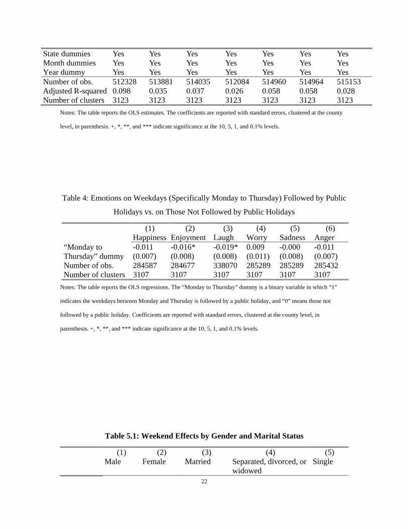
Table 4: Emotions on Weekdays (Specifically Monday to Thursday) Followed by Public

Holidays vs. on Those Not Followed by Public Holidays

(1) (2) (3) (4) (5) (6) Happiness Enjoyment Laugh Worry Sadness Anger “Monday to Thursday” dummy

-0.011 -0.016* -0.019* 0.009 -0.000 -0.011 (0.007) (0.008) (0.008) (0.011) (0.008) (0.007)

Number of obs. 284587 284677 338070 285289 285289 285432 Number of clusters 3107 3107 3107 3107 3107 3107

Notes: The table reports the OLS regressions. The “Monday to Thursday” dummy is a binary variable in which “1”

indicates the weekdays between Monday and Thursday is followed by a public holiday, and “0” means those not

followed by a public holiday. Coefficients are reported with standard errors, clustered at the county level, in

parenthesis. +, *, **, and *** indicate significance at the 10, 5, 1, and 0.1% levels.

Table 5.1: Weekend Effects by Gender and Marital Status

(1) (2) (3) (4) (5) Male Female Married Separated, divorced, or

widowed Single

23

Happiness 0.032*** 0.024*** 0.028*** 0.026*** 0.028*** (0.002) (0.002) (0.001) (0.003) (0.003) Enjoyment 0.051*** 0.050*** 0.053*** 0.047*** 0.047*** (0.002) (0.002) (0.002) (0.003) (0.003) Laughter 0.032*** 0.029*** 0.035*** 0.024*** 0.024*** (0.002) (0.002) (0.002) (0.003) (0.003) Worry -0.069*** -0.072*** -0.077*** -0.060*** -0.061*** (0.002) (0.002) (0.002) (0.004) (0.004) Sadness -0.015*** -0.017*** -0.018*** -0.013** -0.015*** (0.002) (0.002) (0.002) (0.003) (0.003) Anger -0.038*** -0.028*** -0.035*** -0.033*** -0.029*** (0.002) (0.002) (0.002) (0.003) (0.003)

Notes: The table reports the OLS estimates of weekend effects. Each cell of the table presents the weekend effect for a

specific population group and one of the six emotion variables. The control variables in each model include age, age

squared divided by 100, education, employment status, health insurance enrollment status, number of children,

importance of religion in life, as well as state, month and year dummies. Specifically, the marital status is controlled in

the regressions for subpopulations defined by gender, and the gender variable in the regressions for subpopulation

defined by marital status. All the coefficients of these control variables are not reported in the table to save space.

Standard errors, clustered at the county level, are reported in parenthesis. +, *, **, and *** indicate significance at the

10, 5, 1, and 0.1% levels.

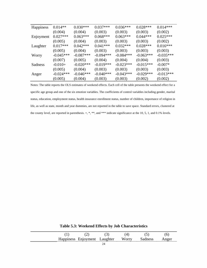
Table 5.2: Weekend Effects by Age Cohort

(1) (2) (3) (4) (5) (6) <=25 26-35 36-45 46-55 56-65 >65

24

Happiness 0.014** 0.030*** 0.037*** 0.036*** 0.028*** 0.014*** (0.004) (0.004) (0.003) (0.003) (0.003) (0.002) Enjoyment 0.027*** 0.063*** 0.068*** 0.063*** 0.044*** 0.025*** (0.005) (0.004) (0.003) (0.003) (0.003) (0.002) Laughter 0.017*** 0.042*** 0.041*** 0.032*** 0.028*** 0.016*** (0.005) (0.004) (0.003) (0.003) (0.003) (0.003) Worry -0.045*** -0.087*** -0.094*** -0.084*** -0.063*** -0.035*** (0.007) (0.005) (0.004) (0.004) (0.004) (0.003) Sadness -0.010+ -0.020*** -0.019*** -0.023*** -0.015*** -0.007* (0.005) (0.004) (0.003) (0.003) (0.003) (0.003) Anger -0.024*** -0.046*** -0.040*** -0.043*** -0.029*** -0.013*** (0.005) (0.004) (0.003) (0.003) (0.002) (0.002)

Notes: The table reports the OLS estimates of weekend effects. Each cell of the table presents the weekend effect for a

specific age group and one of the six emotion variables. The coefficients of control variables including gender, marital

status, education, employment status, health insurance enrollment status, number of children, importance of religion in

life, as well as state, month and year dummies, are not reported in the table to save space. Standard errors, clustered at

the county level, are reported in parenthesis. +, *, **, and *** indicate significance at the 10, 5, 1, and 0.1% levels.

Table 5.3: Weekend Effects by Job Characteristics

(1) (2) (3) (4) (5) (6) Happiness Enjoyment Laughter Worry Sadness Anger

25

Full-time paid worker

0.035*** 0.066*** 0.034*** -0.086*** -0.016*** -0.046*** (0.002) (0.002) (0.002) (0.003) (0.002) (0.002)

Others

0.021*** 0.036*** 0.026*** -0.056*** -0.016*** -0.022*** (0.002) (0.002) (0.002) (0.002) (0.002) (0.002)

Partner-like supervisor

0.024*** 0.047*** 0.026*** -0.078*** -0.011*** -0.032*** (0.001) (0.002) (0.002) (0.002) (0.002) (0.001)

Boss-like supervisor

0.053*** 0.096*** 0.052*** -0.092*** -0.024*** -0.055*** (0.002) (0.003) (0.003) (0.003) (0.003) (0.003)

Trustable workplace

0.022*** 0.045*** 0.022*** -0.073*** -0.011*** -0.031*** (0.002) (0.002) (0.002) (0.003) (0.002) (0.002)

Non-trustable workplace

0.069*** 0.124*** 0.068*** -0.107*** -0.036*** -0.075*** (0.004) (0.004) (0.005) (0.005) (0.005) (0.005)

Satisfied with job

0.022*** 0.044*** 0.024*** -0.076*** -0.014*** -0.034*** (0.002) (0.002) (0.002) (0.003) (0.002) (0.002)

Not satisfied with job

0. 095*** 0.158*** 0.085*** -0.116*** -0.051** -0.090*** (0.008) (0.008) (0.008) (0.009) (0.008) (0.008)

Notes: The table reports the OLS estimates of weekend effects. Each cell of the table presents the weekend effect for a

specific population group and one of the six emotion variables. The coefficients of control variables including age, age

squared divided by 100, gender, marital status, education, employment status, health insurance enrollment status,

number of children, importance of religion in life, as well as state, month and year dummies, are not reported in the

table to save space. Standard errors, clustered at the county level, are reported in parenthesis. +, *, **, and *** indicate

significance at the 10, 5, 1, and 0.1% levels.

Table 6: Weekend Effects Explained by Social Hours

(1) (2) (3) (4) (5) (6)

26

Happiness Enjoyment Laughter Worry Sadness Anger Weekend effects

0.028*** 0.051*** 0.031*** -0.071*** -0.017*** -0.033*** (0.001) (0.001) (0.002) (0.002) (0.001) (0.001)

Log of social hours

0.017*** 0.022*** 0.023*** -0.016*** -0.010*** -0.006*** (0.000) (0.000) (0.000) (0.000) (0.000) (0.000)

Notes: The table reports Blinder-Oaxaca decomposition results. The control variables include age, age squared divided

by 100, gender, marital status, education, employment status, health insurance enrollment status, number of children,

importance of religion in life, log of social hours, indicator for zero social hour, indicator for zero to one social hour,

partner-like supervisor dummy (=1 if supervisor being considered as a partner, and =0 if supervisor being considered as

a boss, value missing or not applicable), boss-like supervisor dummy (=1 if supervisor being considered as a boss, and

=0 if supervisor being considered as a partner, value missing or not applicable), trustable workplace environment (=1 if

reporting trustable workplace environment, =0 if reporting non-trustable workplace environment, value missing or not

applicable), non-trustable workplace environment (=1 if reporting non-trustable workplace environment, =0 if reporting

trustable workplace environment, value missing or not applicable), as well as state, month and year dummies. The

“Weekend effects” indicates the difference of emotions between weekends (including public holidays) and weekdays.

The coefficients of log of social hours are reported with standard errors, clustered at the county level, in parenthesis.

The coefficients of other controls are not reported to save space. +, *, **, and *** indicate significance at the 10, 5, 1,

and 0.1% levels.

Table 7: Sample Means during Weekends and Weekdays

Weekends Weekdays

27

Variables # obs Mean S.E. #obs Mean S.E. Log of income 165060 6.257 (0.011) 362221 6.249 (0.007)Indicator for no or missing income 165060 0.232 (0.001) 362221 0.232 (0.001)Male 165060 0.483 (0.002) 362221 0.483 (0.001)Age 163163 47.972 (0.055) 358032 48.045 (0.037)Age-squared/100 163163 26.047 (0.053) 358032 26.137 (0.036) Married or as married 164699 0.583 (0.002) 361418 0.581 (0.001)Separated, divorced, or windowed 164699 0.208 (0.001) 361418 0.210 (0.001)High school 164449 0.364 (0.002) 360721 0.362 (0.001)Some college 164449 0.220 (0.001) 360721 0.221 (0.001)College 164449 0.167 (0.001) 360721 0.167 (0.002)Graduate 164449 0.130 (0.001) 360721 0.131 (0.001)Full-time paid worker 165060 0.469 (0.002) 362221 0.459 (0.001)Part-time paid worker 165060 0.109 (0.001) 362221 0.109 (0.001)Health insurance 164857 0.849 (0.001) 361756 0.846 (0.001)Number of children 164810 0.750 (0.004) 361746 0.749 (0.003)Importance of religion in life 164373 0.659 (0.001) 360689 0.654 (0.001)Social hours 163996 7.158 (0.015) 359399 5.420 (0.010)Indicator for no social hour 163996 0.051 (0.001) 359399 0.057 (0.000)Indicator for zero to one social hour

163996 0.021 (0.000) 359399 0.033 (0.000)

Partner-like supervisor 81199 0.639 (0.002) 169902 0.646 (0.001)Trustable workplace 81571 0.796 (0.002) 170704 0.793 (0.001)Satisfied with job 70484 0.897 (0.001) 146026 0.894 (0.001)

Note: Standard errors clustered at the county level are reported in parenthesis.

Table 8: Sources of Weekend Effects: Workplace Environment

(1) (2) (3) (4)

28

Partner-like supervisor Trustable and open workplace Weekends Weekdays Weekends Weekdays Panel 1: Sample Means Mean 0.639*** 0.646*** 0.796*** 0.793*** (0.002) (0.001) (0.002) (0.001)

Panel 2: Coefficients Happiness 0.033*** 0.058*** 0.052*** 0.095*** (0.003) (0.002) (0.003) (0.003) Enjoyment 0.042*** 0.083*** 0.070*** 0.144*** (0.003) (0.002) (0.004) (0.003) Laugh 0.051*** 0.076*** 0.074*** 0.117*** (0.003) (0.002) (0.004) (0.003) Worry -0.074*** -0.086*** -0.123*** -0.154*** (0.004) (0.003) (0.005) (0.004) Sadness -0.035*** -0.048*** -0.061*** -0.086*** (0.003) (0.002) (0.004) (0.003) Anger -0.040*** -0.057*** -0.072*** -0.116*** (0.003) (0.003) (0.004) (0.003)

Notes: The table reports the sample means (in panel 1) and marginal effects (in panel 2) of two variables indicating

workplace environment during weekdays and weekends. Each cell of panel 2 in model (1) and (2) presents the marginal

effect of the dummy variable indicating “supervisor being considered a partner rather than a boss” for one of the six

emotion variables. Each cell of panel 2 in model (3) and (4) presents the marginal effect of the dummy variable

indicating “trustable and open workplace environment” for one of the six emotion variables. The control variables in

the regressions include age, age squared divided by 100, gender, marital status, education, employment status, health

insurance enrollment status, number of children, importance of religion in life, as well as state, month and year

dummies. Standard errors clustered at the county level are reported in parenthesis. +, *, **, and *** indicate

significance at the 10, 5, 1, and 0.1% levels.

29

-0.120 -0.100 -0.080 -0.060 -0.040 -0.020 0.000 0.020 0.040 0.060 0.080

Figure 1: The Cantril Ladder and EmotionsMean Differences from Monday

Tue-Mon Wed-Mon Thu-MonFri-Mon Sat-Mon Sun-MonHoliday-Mon

-0.100

-0.050

0.000

0.050

0.100

0.150

Figure 2: The Cantril Ladder and EmotionsDay-of-Week Effects

Tue Wed Thu Fri Sat Sun Public Holiday

30

-0.100

-0.080

-0.060

-0.040

-0.020

0.000

0.020

0.040

0.060

0.080

Happiness Enjoyment Laughter Worry Sadness Anger

Figure 3.1: Weekend Effects by Gender and Marital Status

Male Female Married Single Separated, divorced, or widowed

-0.120 -0.100 -0.080 -0.060 -0.040 -0.020 0.000 0.020 0.040 0.060 0.080 0.100

Happiness Enjoyment Laughter Worry Sadness Anger

Figure 3.2: Weekend Effects by Age Cohort

Age<=25 25<Age<=35 35<Age<=45

45<Age<=55 55<Age<=65 Age>65

31

-0.160

-0.120

-0.080

-0.040

0.000

0.040

0.080

0.120

0.160

0.200

Happiness Enjoyment Laughter Worry Sadness Anger

Figure 3.3: Weekend Effects by Job Characteristics

Full-time paid workers Others

Partner-like Supervisor Boss-like Supervisor

Trustable workplace Non-trustable workplace

Satisfied with job Not satisfied with job

-0.100

-0.080

-0.060

-0.040

-0.020

0.000

0.020

0.040

0.060

Happiness Enjoyment Laughter Worry Sadness Anger

Figure 4: Oaxaca DecompostionWeekend Effects Explained by Social Hours

Weekend effects Log of social hours

32

-0.200

-0.150

-0.100

-0.050

0.000

0.050

0.100

0.150

Happiness Enjoyment Laughter Worry Sadness Anger

Figure 5: Marginal Effect of Workplace Environment on Weekends and Weekdays

Partner-like Supervisor: Weekends

Partner-like Supervisor: Weekdays

Trustable and open workplace: Weekends

Trustable and open workplace: Weekdays