weighted extremal domains and best … extremal domains and best rational approximation laurent...

WEIGHTED EXTREMAL DOMAINS AND BEST RATIONALAPPROXIMATION

LAURENT BARATCHART, HERBERT STAHL, AND MAXIM YATTSELEV

Abstract. Let f be holomorphically continuable over the complex plane except for

finitely many branch points contained in the unit disk. We prove that best rationalapproximants to f of degree n, in the L2-sense on the unit circle, have poles that asymp-

totically distribute according to the equilibrium measure on the compact set outside of

which f is single-valued and which has minimal Green capacity in the disk among allsuch sets. This provides us with n-th root asymptotics of the approximation error. By

conformal mapping, we deduce further estimates in approximation by rational or mero-

morphic functions to f in the L2-sense on more general Jordan curves encompassing thebranch points. The key to these approximation-theoretic results is a characterization of

extremal domains of holomorphy for f in the sense of a weighted logarithmic potential,

which is the technical core of the paper.

List of Symbols

Sets:C extended complex planeT Jordan curve with exterior domain O and interior domain GT unit circle with exterior domain O and interior domain DEf set of the branch points of fK∗ reflected set z : 1/z ∈ KK set of minimal condenser capacity in Kf (G)Γν and Dν minimal set for Problem (f, ν) and its complement in C(Γ)ε z ∈ D : dist(z,Γ) < εγu image of a set γ under 1/(· − u)Collections:Kf (G) admissible sets for f ∈ A(G), Kf = Kf (D)Gf admissible sets in Kf comprised of a finite number of continuaΛ(F ) probability measures on F

2000 Mathematics Subject Classification. 42C05, 41A20, 41A21.Key words and phrases. rational approximation, meromorphic approximation, extremal domains, weak

asymptotics, non-Hermitian orthogonality.The research of first and the third authors was partially supported by the ANR project “AHPI” (ANR-

07-BLAN-0247-01). The research of the second author has been supported by the Deutsche Forschungsge-meinschaft (AZ: STA 299/13-1).

1

2 L. BARATCHART, H. STAHL, AND M. YATTSELEV

Spaces:Pn algebraic polynomials of degree at most nMn(G) monic algebraic polynomials of degree n with n zeros in G, Mn =Mn(D)Rn(G) Rn(G) := Pn−1M−1

n (G), Rn = Rn(D)A(G) holomorphic functions C except for branch-type singularities in GLp(T ) classical Lp spaces, p <∞, with respect to arclength on T and the norm ‖ · ‖p,T‖ · ‖K supremum norm on a set KE2(G) Smirnov class of holomorphic functions in G with L2 traces on TE2n(G) E2

n(G) := E2(G)M−1n (G)

H2 classical Hardy space of holomorphic functions in D with L2 traces on TH2n H2

n := H2M−1n

Measures:ω∗ reflected measure, ω∗(B) = ω(B∗)ω or ω balayage of ω, supp(ω) ⊂ D, onto ∂DωF equilibrium distribution on FωF,ψ weighted equilibrium distribution on F in the field ψω(F,E) Green equilibrium distribution on F relative to C \ ECapacities:cap(K) logarithmic capacity of Kcapν(K) ν-capacity of Kcap(E,F ) capacity of the condenser (E,F )Energies:I[ω] logarithmic energy of ωIψ[ω] weighted logarithmic energy of ω in the field ψID[ω] Green energy of ω relative to DIν [K] ν-energy of a set KDD(u, v) Dirichlet integral of functions u, v in a domain D

Potentials:V ω logarithmic potential of ωV ω∗ spherical logarithmic potential of ωUν spherically normalized logarithmic potential of ν∗

V ωD Green potential of ω relative to DgD(·, u) Green function for D with pole at uConstants:c(ψ;F ) modified Robin constant, c(ψ;F ) = Iψ[ωF,ψ]−

∫ψdωF,ψ

c(ν;D) is equal to∫gD(z,∞)dν(z) if D is unbounded and to 0 otherwise

1. Introduction

Approximation theory in the complex domain has undergone striking developments overthe last years that gave new impetus to this classical subject. After the solution to theGonchar conjecture [39, 44] and the achievement of weak asymptotics in Pade approxima-tion [48, 50, 25] came the disproof of the Baker-Gammel-Wills conjecture [36, 15], and theRiemann-Hilbert approach to the limiting behavior of orthogonal polynomials [18, 31] thatopened the way to unprecedented strong asymptotics in rational interpolation [4, 3, 14] (see[17, 30] for other applications of this powerful device). Meanwhile, the spectral approach tomeromorphic approximation [1], already instrumental in [39], has produced sharp conversetheorems in rational approximation and fueled engineering applications to control systemsand signal processing [23, 41, 38, 40].

RATIONAL APPROXIMANTS TO ALGEBRAIC FUNCTIONS 3

In most investigations involved with non-Hermitian orthogonal polynomials and rationalinterpolation, a central role has been played by certain geometric extremal problems fromlogarithmic potential theory, close in spirit to the Lavrentiev type [32], that were introducedin [49]. On the one hand, their solution produces systems of arcs over which non-Hermitianorthogonal polynomials can be analyzed; on the other hand such polynomials are preciselydenominators of rational interpolants to functions that may be expressed as Cauchy integralsover this system of arcs, the interpolation points being chosen in close relation with the latter.

One issue facing now the theory is to extend to best rational or meromorphic approximantsof prescribed degree to a given function the knowledge that was gained about rationalinterpolants. Optimality may of course be given various meanings. However, in view ofthe connections with interpolation theory pointed out in [35, 11, 12], and granted theirrelevance to spectral theory, the modeling of signals and systems, as well as inverse problems[2, 22, 28, 37, 10, 29, 46], it is natural to consider foremost best approximants in Hardyclasses.

The main interest there attaches to the behavior of the poles whose determination is thenon-convex and most difficult part of the problem. The first obstacle to value interpolationtheory in this context is that it is unclear whether best approximants of a given degreeshould interpolate the function at enough points, and even if they do these interpolationpoints are no longer parameters to be chosen adequately in order to produce convergence butrather unknown quantities implicitly determined by the optimality property. The presentpaper deals with H2-best rational approximation in the complement of the unit disk, forwhich maximum interpolation is known to take place; it thus remains in this case to locatethe interpolation points. This we do asymptotically, when the degree of the approximantgoes large, for functions whose singularities consist of finitely many poles and branch pointsin the disk. More precisely, we prove that the normalized (probability) counting measuresof the poles of the approximants converge, in the weak star sense, to the equilibrium dis-tribution of the continuum of minimum Green capacity, in the disk, outside of which theapproximated function is single-valued. By conformal mapping, the result carries over tobest meromorphic approximants with a prescribed number of poles, in the L2-sense on a Jor-dan curve encompassing the poles and branch points. We also estimate the approximationerror in the n-th root sense, that turns out to be the same as in uniform approximation forthe functions under consideration. Note that H2-best rational approximants on the disk areof fundamental importance in stochastic identification [28] and that functions with branchpoints arise naturally in inverse sources and potential problems [7, 9], so the result may beregarded as a prototypical case of the above-mentioned program.

The paper is organized as follows. In Sections 2 and 3, we fix the terminology andrecall some known facts about H2-best rational approximants and sets of minimal condensercapacity, before stating our main results (Theorems 5 and 7) along with some corollaries.We set up in Section 4 a weighted version of the extremal potential problem introduced in[49] (cf. Definition 9) and stress its main features. Namely, a solution exists uniquely andcan be characterized, among continua outside of which the approximated function is single-valued, as a system of arcs possessing the so-called S-property in the field generated by theweight (cf. Definition 10 and Theorem 12). Section 5 is a brief introduction to multipointPade interpolants, of which H2-best rational approximants are a particular case. Section 6contains the proofs of all the results: first we establish Theorem 12, which is the technicalcore of the paper, using compactness properties of the Hausdorff metric together with thea priori geometric estimate of Lemma 17 to prove existence; the S-property is obtainedby showing the local equivalence of our weighted extremal problem with one of minimal


condenser capacity (Lemma 19); uniqueness then follows from a variational argument usingDirichlet integrals (Lemma 20). After Theorem 12 is established, the proof of Theorem 7 isnot too difficult. We choose as weight (minus) the potential of a limit point of the normalizedcounting measures of the interpolation points of the approximants and, since we now knowthat a compact set of minimal weighted capacity exists and that it possesses the S-property,we can adapt results from [25] to the effect that the normalized counting measures of thepoles of the approximants converge to the weighted equilibrium distribution on this systemof arcs. To see that this is nothing but the Green equilibrium distribution, we appeal to thefact that poles and interpolation points are reflected from each other across the unit circlein H2-best rational approximation. The results carry over to more general domains as inTheorem 5 by a conformal mapping (Theorem 6). The appendix in Section 7 gathers sometechnical results from logarithmic potential theory that are needed throughout the paper.

2. Rational Approximation in L2

In this work we are concerned with rational approximation of functions analytic at in-finity having multi-valued meromorphic continuation to the entire complex plane deprivedof a finite number of points. The approximation will be understood in the L2-norm on arectifiable Jordan curve encompassing all the singularities of the approximated function.Namely, let T be such a curve. Let further G and O be the interior and exterior domains ofT , respectively, i.e., the bounded and unbounded components of the complement of T in theextended complex plane C. We denote by L2(T ) the space of square-summable functions onT endowed with the usual norm

‖f‖22,T :=∫T

|f |2ds,

where ds is the arclength differential. Set Pn to be the space of algebraic polynomials ofdegree at most n and Mn(G) to be its subset consisting of monic polynomials with n zerosin G. Define

(2.1) Rn(G) :=p(z)q(z)

=pn−1z

n−1 + pn−2zn−2 + · · ·+ p0

zn + qn−1zn−1 + · · ·+ q0: p ∈ Pn−1, q ∈Mn(G)

.

That is, Rn(G) is the set of rational functions with at most n poles that are holomorphicin some neighborhood of O and vanish at infinity. Let f be a function holomorphic andvanishing at infinity (vanishing at infinity is a normalization required for convenience only).We say that f belongs to the class A(G) if

(i) f admits holomorphic and single-valued continuation from infinity to an open neigh-borhood of O;

(ii) f admits meromorphic, possibly multi-valued, continuation along any arc in G \Efstarting from T , where Ef is a finite set of points in G;

(iii) Ef is non-empty, the meromorphic continuation of f from infinity has a branchpoint at each element of Ef .

The primary example of functions in A(G) is that of algebraic functions. Every algebraicfunction f naturally defines a Riemann surface. Fixing a branch of f at infinity is equivalentto selecting a sheet of this covering surface. If all the branch points and poles of f on thissheet lie above G, the function f belongs to A(G). Other functions in A(G) are those ofthe form g log(l1/l2) + r, where g is entire and l1, l2 ∈ Mm(G) while r ∈ Rk(G) for somem, k ∈ N. However, A(G) is defined in such a way that it contains no function in Rn(G),n ∈ N, in order to avoid degenerate cases.


With the above notation, the goal of this section is to describe the asymptotic behaviorof

(2.2) ρn,2(f, T ) := inf ‖f − r‖2,T : r ∈ Rn(G) , f ∈ A(G).

This problem is, in fact, a variation of a classical question in Chebyshev (uniform) rationalapproximation of holomorphic functions where it is required to describe the asymptoticbehavior of

ρn,∞(f, T ) := inf ‖f − r‖T : r ∈ Rn(G) ,where ‖ · ‖T is the supremum norm on T . The theory behind Chebyshev approximation israther well established while its L2-counterpart, which naturally arises in system identifi-cation and control theory [5] and serves as a method to approach inverse source problems[7, 9, 10], is not so much developed. In particular, it follows from the techniques of rationalinterpolation devised by Walsh [54] that

(2.3) lim supn→∞

ρ1/nn,∞(f, T ) ≤ exp

− 1

cap(K,T )

for any function f holomorphic outside of K ⊂ G, where cap(K,T ) is the condenser capacity(Section 7.1.3) of a set K contained in a domain G relative to this domain1. On the otherhand, it was conjectured by Gonchar and proved by Parfenov [39, Sec. 5] on simply connecteddomains, also later by Prokhorov [44] in full generality, that

(2.4) lim infn→∞

ρ1/2nn,∞ (f, T ) ≤ exp

− 1

cap(K,T )

.

Notice that only the n-th root is taken in (2.3) while (2.4) provides asymptotics for the2n-th root. Observe also that there are many compacts K which make a given f ∈ A(G)single-valued in their complement. Hence, (2.3) and (2.4) can be sharpened by taking theinfimum over K on the right-hand side of both inequalities. To explore this fact we needthe following definition.

Definition 1. We say that a compact K ⊂ G is admissible for f ∈ A(G) if C \ K isconnected and f has meromorphic and single-valued extension there. The collection of alladmissible sets for f we denote by Kf (G).

As equations (2.3) and (2.4) suggest and Theorem 5 below shows, the relevant admissibleset in rational approximation to f ∈ A(G) is the set of minimal condenser capacity [48, 49,50, 51] relative to G:

Definition 2. Let f ∈ A(G). A compact K ∈ Kf (G) is said to be a set of minimal condensercapacity for f if

(i) cap(K, T ) ≤ cap(K,T ) for any K ∈ Kf (G);(ii) K ⊂ K for any K ∈ Kf (G) such that cap(K,T ) = cap(K, T ).

It follows from the properties of condenser capacity that cap(K, T ) = cap(T,K) =cap(O,K) since K has connected complement that contains T by Definition 1. In otherwords, the set K can be seen as the complement of the “largest” (in terms of capacity)domain containing O on which f is single-valued and meromorphic. In fact, this is exactlythe point of view taken up in [48, 49, 50, 51]. It is known that such a set always exists, is

1In Section 7 the authors provide a concise but self-contained account of logarithmic potential theory.The reader may want to consult this section to get accustomed with the employed notation for capacities,

energies, potentials, and equilibrium measures.


unique, and has, in fact, a rather special structure. To describe it, we need the followingdefinition.

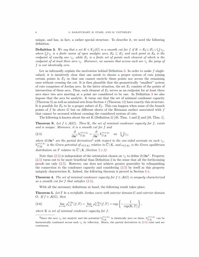
Definition 3. We say that a set K ∈ Kf (G) is a smooth cut for f if K = E0 ∪ E1 ∪⋃γj,

where⋃γj is a finite union of open analytic arcs, E0 ⊆ Ef and each point in E0 is the

endpoint of exactly one γj, while E1 is a finite set of points each element of which is theendpoint of at least three arcs γj. Moreover, we assume that across each arc γj the jump off is not identically zero.

Let us informally explain the motivation behind Definition 3. In order to make f single-valued, it is intuitively clear that one needs to choose a proper system of cuts joiningcertain points in Ef so that one cannot encircle these points nor access the remainingones without crossing the cut. It is then plausible that the geometrically “smallest” systemof cuts comprises of Jordan arcs. In the latter situation, the set E1 consists of the points ofintersection of these arcs. Thus, each element of E1 serves as an endpoint for at least threearcs since two arcs meeting at a point are considered to be one. In Definition 3 we alsoimpose that the arcs be analytic. It turns out that the set of minimal condenser capacity(Theorem S) as well as minimal sets from Section 4 (Theorem 12) have exactly this structure.It is possible for E0 to be a proper subset of Ef . This can happen when some of the branchpoints of f lie above G but on different sheets of the Riemann surface associated with fthat cannot be accessed without crossing the considered system of cuts.

The following is known about the set K (Definition 2) [48, Thm. 1 and 2] and [49, Thm. 1].

Theorem S. Let f ∈ A(G). Then K, the set of minimal condenser capacity for f , existsand is unique. Moreover, it is a smooth cut for f and

(2.5)∂

∂n+Vω(T,K)

C\K =∂

∂n−Vω(T,K)

C\K on⋃γj ,

where ∂/∂n± are the partial derivatives2 with respect to the one-sided normals on each γj,Vω(T,K)

C\K is the Green potential of ω(T,K) relative to C\K, and ω(T,K) is the Green equilibrium

distribution on T relative to C \K (Section 7.1.3).

Note that (2.5) is independent of the orientation chosen on γj to define ∂/∂n±. Property(2.5) turns out to be more beneficial than Definition 2 in the sense that all the forthcomingproofs use only (2.5). However, one does not achieve greater generality by relinquishingthe connection to the condenser capacity and considering (2.5) by itself as this propertyuniquely characterizes K. Indeed, the following theorem is proved in Section 6.4.

Theorem 4. The set of minimal condenser capacity for f ∈ A(G) is uniquely characterizedas a smooth cut for f that satisfies (2.5).

With all the necessary definitions at hand, the following result takes place.

Theorem 5. Let T be a rectifiable Jordan curve with interior domain G and exterior domainO. If f ∈ A(G), then

(2.6) limn→∞

ρ1/2nn,2 (f, T ) = lim

n→∞ρ1/2nn,∞ (f, T ) = exp

− 1

cap(K, T )

,

where K is set of minimal condenser capacity for f .

2Since the arcs γj are analytic and the potential Vω(T,K)

C\Kis identically zero on them, V

ω(T,K)

C\Kcan be

harmonically continued across each γj by reflection. Hence, the partial derivatives in (2.5) exist and are

continuous.


The second equality in (2.6) follows from [25, Thm 1′], where a larger class of functionsthan A(G) is considered (see Theorem GR in Section 6.3). To prove the first equality, weappeal to another type of approximation, namely, meromorphic approximation in L2-normon T , for which asymptotics of the error and the poles are obtained below. This type ofapproximation turns out to be useful in certain inverse source problems [9, 34, 16]. Observethat |T |1/p−1/2‖h‖2,T ≤ ‖h‖p,T ≤ |T |1/p‖h‖T for any p ∈ (2,∞) and any bounded functionh on T by Holder inequality, where ‖ · ‖p,T is the usual p-norm on T with respect to ds and|T | is the arclength of T . Thus, Theorem 5 implies that (2.6) holds for Lp(T )-best rationalapproximants as well when p ∈ (2,∞). In fact, as Vilmos Totik pointed out to the authors[53], with a different method of proof Theorem 5 can be extended to include the full rangep ∈ [1,∞].

Just mentioned best meromorphic approximants are defined as follows. Denote by E2(G)the Smirnov class3 for G [20, Sec. 10.1]. It is known that functions in E2(G) have non-tangential boundary values a.e. on T and thus formed traces of functions in E2(G) belongto L2(T ). Now, put E2

n(G) := E2(G)M−1n (G) to be the set of meromorphic functions in G

with at most n poles there and square-summable traces on T . It is known [10, Sec. 5] thatfor each n ∈ N there exists gn ∈ E2

n(G) such that

‖f − gn‖2,T = inf‖f − g‖2,T : g ∈ E2

n(G).

That is, gn is a best meromorphic approximant for f in the L2-norm on T .

Theorem 6. Let T be a rectifiable Jordan curve with interior domain G and exterior domainO. If f ∈ A(G), then

(2.7) |f − gn|1/2ncap→ exp

Vω(K,T )

G − 1cap(K, T )

in G \K,

where the functions gn ∈ E2n(G) are best meromorphic approximants to f in the L2-norm on

T , K is the set of minimal condenser capacity for f in G, ω(K,T ) is the Green equilibriumdistribution on K relative to G, and

cap→ denotes convergence in capacity (see Section 7.1.1).Moreover, the counting measures of the poles of gn converge weak∗ to ω(K,T ).

3. H20 -Rational Approximation

To prove Theorems 5 and 6, we derive a stronger result in the model case where G is theunit disk, D. The strengthening comes from the facts that in this case L2-best meromorphicapproximants specialize to L2-best rational approximants the latter also turn out to beinterpolants. In fact, we consider not only best rational approximants but also criticalpoints in rational approximation.

Let T be the unit circle and set for brevity L2 := L2(T). Denote by H2 ⊂ L2 the Hardyspace of functions whose Fourier coefficients with strictly negative indices are zero. Thespace H2 can be described as the set of traces of holomorphic functions in the unit diskwhose square-means on concentric circles centered at zero are uniformly bounded above4

[20]. Further, denote by H20 the orthogonal complement of H2 in L2, L2 = H2 ⊕ H2

0 , withrespect to the standard scalar product

〈f, g〉 :=∫

Tf(τ)g(τ)|dτ |, f, g ∈ L2.

3A function h belongs to E2(G) if h is holomorphic in G and there exists a sequence of rectifiable Jordancurves, say Tn, whose interior domains exhaust G, such that ‖h‖2,Tn ≤ const. independently of n.

4Each such function has non-tangential boundary values almost everywhere on T and can be recoveredfrom these boundary values by means of the Cauchy or Poisson integral.


From the viewpoint of analytic function theory, H20 can be regarded as a space of traces

of functions holomorphic in O := C \ D and vanishing at infinity whose square-means onthe concentric circles centered at zero (this time with radii greater then 1) are uniformlybounded above. In what follows, we denote by ‖ · ‖2 the norm on L2 induced by the scalarproduct 〈·, ·〉. In fact, ‖ · ‖2 is a norm on H2 and H2

0 as well.We setMn :=Mn(D) andRn := Rn(D). Observe thatRn is the set of rational functions

of degree at most n belonging to H20 . With the above notation, consider the following H2

0 -rational approximation problem:Given f ∈ H2

0 and n ∈ N, minimize ‖f − rn‖2 over all r ∈ Rn.It is well-known (see [6, Prop. 3.1] for the proof and an extensive bibliography on thesubject) that this minimum is always attained while any minimizing rational function, alsocalled a best rational approximant to f , lies in Rn \ Rn−1 unless f ∈ Rn−1.

Best rational approximants are part of the larger class of critical points in H20 -rational

approximation. From the computational viewpoint, critical points are as important as bestapproximants since a numerical search is more likely to yield a locally best rather than abest approximant. For fixed f ∈ H2

0 , critical points can be defined as follows. Set

(3.1)Ψf,n : Pn−1 ×Mn → [0,∞)

(p, q) 7→ ‖f − p/q‖22.

In other words, Ψf,n is the squared error of approximation of f by r = p/q in Rn. Wetopologically identify Pn−1 ×Mn with an open subset of C2n with coordinates pj and qk,j, k ∈ 0, . . . , n−1 (see (2.1)). Then a pair of polynomials (pc, qc) ∈ Pn−1×Mn, identifiedwith a vector in C2n, is said to be a critical pair of order n, if all the partial derivatives of Ψf,n

do vanish at (pc, qc). Respectively, a rational function rc ∈ Rn is a critical point of order n ifit can be written as the ratio rc = pc/qc of a critical pair (pc, qc) in Pn−1×Mn. A particularexample of a critical point is a locally best approximant. That is, a rational function rl = pl/qlassociated with a pair (pl, ql) ∈ Pn−1 ×Mn such that Ψf,n(pl, ql) ≤ Ψf,n(p, q) for all pairs(p, q) in some neighborhood of (pl, ql) in Pn−1 ×Mn. We call a critical point of order nirreducible if it belongs to Rn \ Rn−1. As we have already mentioned, best approximants,as well as local minima, are always irreducible critical points unless f ∈ Rn−1. In generalthere may be other critical points, reducible or irreducible, which are saddles or maxima. Infact, to give amenable conditions for uniqueness of a critical point it is a fairly open problemof great practical importance, see [5, 11, 13] and the bibliography therein.

One of the most important properties of critical points is the fact that they are “maximal”rational interpolants. More precisely, let f ∈ H2

0 and rn be an irreducible critical point oforder n, then rn interpolates f at the reflection (z 7→ 1/z) of each pole of rn with order twicethe multiplicity that pole [35], [13, Prop. 2], which is the maximal number of interpolationconditions (i.e., 2n) that can be imposed in general on a rational function of type (n− 1, n)(i.e., the ratio of a polynomial of degree n− 1 by a polynomial of degree n).

With all the definitions at hand, we are ready to state our main results concerning thebehavior of critical points in H2

0 -rational approximation for functions in A(D), which willbe proven in Section 6.4.

Theorem 7. Let f ∈ A(D) and rnn∈N be a sequence of irreducible critical points in H20 -

rational approximation for f . Further, let K be the set of minimal condenser capacity forf . Then the normalized counting measures5 of the poles of rn converge weak∗ to the Green

5The normalized counting measure of poles/zeros of a given function is a probability measure havingequal point masses at each pole/zero of the function counting multiplicity.


equilibrium distribution on K relative to D, ω(K,T). Moreover, it holds that

(3.2) |(f − rn)|1/2n cap→ exp−V ω

∗(K,T)

C\K

in C \ (K ∪K∗),

where K∗ and ω∗(K,T) are the reflections6 of K and ω(K,T) across T, respectively, andcap→

denotes convergence in capacity. In addition, it holds that


|(f − rn)(z)|1/2n ≤ exp−V ω

∗(K,T)

C\K (z)

uniformly for z ∈ O.

Using the fact that the Hardy space H2 is orthogonal to H20 , one can show that L2-best

meromorphic approximants discussed in Theorem 6 specialize to L2-best rational approxi-mants when G = D (see the proof of Theorem 6). Moreover, it is shown in Lemma 25 in

Section 7 that −V ω∗(K,T)

C\K ≡ V ω(K,T)

D − 1/cap(K,T) in D. So, formula (2.7) is, in fact, a gener-

alization of (3.2), but only in G \K. Lemma 25 also implies that Vω∗(K,T)

C\K ≡ 1/cap(K,T) onT. In particular, the following corollary to Theorem 7 can be stated.

Corollary 8. Let f , rn, and K be as in Theorem 7. Then

(3.4) limn→∞

‖f − rn‖1/2n2 = limn→∞

‖f − rn‖1/2nT = exp− 1

cap(K,T)

,

where ‖ · ‖T stands for the supremum norm on T.

Observe that Corollary 8 strengthens Theorem 5 in the case when T = T. Indeed,(3.4) combined with (2.6) implies that the critical points in H2

0 -rational approximation alsoprovide the best rate of uniform approximation in the n-th root sense for f on O.

4. Domains of Minimal Weighted Capacity

Our approach to Theorem 7 lies in exploiting the interpolation properties of the criticalpoints in H2

0 -rational approximation. To this end we first study the behavior of rationalinterpolants with predetermined interpolation points (Theorem 14 in Section 5). However,before we are able to touch upon the subject of rational interpolation proper, we need toidentify the corresponding minimal sets. These sets are the main object of investigation inthis section.

Let ν be a probability Borel measure supported in D. We set

(4.1) Uν(z) := −∫

log |1− zu|dν(u).

The function Uν is simply the spherically normalized logarithmic potential of ν∗, the re-flection of ν across T (see (7.1)). Hence, it is a harmonic function outside of supp(ν∗), inparticular, in D. Considering −Uν as an external field acting on non-polar compact subsetsof D, we define the weighted capacity in the usual manner (Section 7.1.2). Namely, for sucha set K ⊂ D, we define the ν-capacity of K by

(4.2) capν(K) := exp −Iν [K] , Iν [K] := minω

(I[ω]− 2

∫Uνdω

),

6For every set K we define the reflected set K∗ as K∗ := z : 1/z ∈ K. If ω is a Borel measure in C,then ω∗ is a measure such that ω∗(B) = ω(B∗) for every Borel set B.


where the minimum is taken over all probability Borel measures ω supported on K (seeSection 7.1.1 for the definition of energy I[·]). Clearly, Uδ0 ≡ 0 and therefore capδ0(·) issimply the classical logarithmic capacity (Section 7.1.1), where δ0 is the Dirac delta at theorigin.

The purpose of this section is to extend results in [48, 49] obtained for ν = δ0. For that,we introduce a notion of a minimal set in a weighted context. This generalization is the keyenabling us to adapt the results of [25] to the present situation, and its study is really thetechnical core of the paper. For simplicity, we put Kf := Kf (D).

Definition 9. Let ν be a probability Borel measure supported in D. A compact Γν ∈ Kf ,f ∈ A(D), is said to be a minimal set for Problem (f, ν) if

(i) capν(Γν) ≤ capν(K) for any K ∈ Kf ;(ii) Γν ⊂ Γ for any Γ ∈ Kf such that cap(Γ) = cap(Γν).

The set Γν will turn out to have geometric properties similar to those of minimal condensercapacity sets (Definition 2). This motivates the following definition.

Definition 10. A compact Γ ∈ Kf is said to be symmetric with respect to a Borel measureω, supp(ω) ∩ Γ = ∅, if Γ is a smooth cut for f (Definition 3) and

(4.3)∂

∂n+V ωC\Γ =

∂

∂n−V ωC\Γ on

⋃γj ,

where ∂/∂n± are the partial derivatives with respect to the one-sided normals on each sideof γj and V ωC\Γ is the Green potential of ω relative to C \ Γ.

Definition 10 is given in the spirit of [49] and thus appears to be different from the S-property defined in [25]. Namely, a compact Γ ⊂ D having the structure of a smooth cut issaid to possess the S-property in the field ψ, assumed to be harmonic in some neighborhoodof Γ, if

(4.4)∂(V ωΓ,ψ + ψ)

∂n+=∂(V ωΓ,ψ + ψ)

∂n−, q. e. on

⋃γj ,

where ωΓ,ψ is the weighted equilibrium distribution on Γ in the field ψ and the normalderivatives exist at every tame point of supp(ωΓ,ψ) (see Section 6.3). It follows from (7.23)and (7.20) that Γ has the S-property in the field −Uν if and only if it is symmetric withrespect to ν∗, taking into account that V ωΓ,−Uν − Uν is constant on the arcs γj which areregular (see Section 7.2.2) hence the normal derivatives exist at every point. This reconcilesDefinition 10 with the one given in [25] in the setting of our work.

The symmetry property (4.3) entails that V ωC\Γ has a very special structure.

Proposition 11. Let Γ = E0 ∪ E1 ∪⋃γj and V ωC\Γ be as in Definitions 3 and 10. Then

the arcs γj possess definite tangents at their endpoints. The tangents to the arcs ending ate ∈ E1 (there are at least three by definition of a smooth cut) are equiangular. Further, set

(4.5) Hω,Γ := ∂zVω

C\Γ, ∂z := (∂x − i∂y)/2.

Then Hω,Γ is holomorphic in C\(Γ∪supp(ω)) and has continuous boundary values from eachside of every γj that satisfy H+

ω,Γ = −H−ω,Γ on each γj. Moreover, H2ω,Γ is a meromorphic

function in C \ supp(ω) that has a simple pole at each element of E0 and a zero at eachelement e of E1 whose order is equal to the number of arcs γj having e as endpoint minus2.


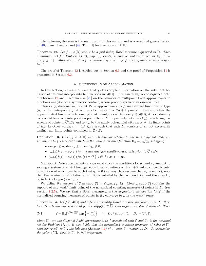
The following theorem is the main result of this section and is a weighted generalizationof [48, Thm. 1 and 2] and [49, Thm. 1] for functions in A(D).

Theorem 12. Let f ∈ A(D) and ν be a probability Borel measure supported in D. Thena minimal set for Problem (f, ν), say Γν , exists, is unique and contained in Dr, r :=maxz∈Ef |z|. Moreover, Γ ∈ Kf is minimal if and only if it is symmetric with respectto ν∗.

The proof of Theorem 12 is carried out in Section 6.1 and the proof of Proposition 11 ispresented in Section 6.2.

5. Multipoint Pade Approximation

In this section, we state a result that yields complete information on the n-th root be-havior of rational interpolants to functions in A(D). It is essentially a consequence bothof Theorem 12 and Theorem 4 in [25] on the behavior of multipoint Pade approximants tofunctions analytic off a symmetric contour, whose proof plays here an essential role.

Classically, diagonal multipoint Pade approximants to f are rational functions of type(n, n) that interpolate f at a prescribed system of 2n + 1 points. However, when theapproximated function is holomorphic at infinity, as is the case f ∈ A(D), it is customaryto place at least one interpolation point there. More precisely, let E = En be a triangularscheme of points in C\Ef and let vn be the monic polynomial with zeros at the finite pointsof En. In other words, E := Enn∈N is such that each En consists of 2n not necessarilydistinct nor finite points contained in C \ Ef .

Definition 13. Given f ∈ A(D) and a triangular scheme E, the n-th diagonal Pade ap-proximant to f associated with E is the unique rational function Πn = pn/qn satisfying:

• deg pn ≤ n, deg qn ≤ n, and qn 6≡ 0;

• (qn(z)f(z)− pn(z)) /vn(z) has analytic (multi-valued) extension to C \ Ef ;

• (qn(z)f(z)− pn(z)) /vn(z) = O(1/zn+1

)as z →∞.

Multipoint Pade approximants always exist since the conditions for pn and qn amount tosolving a system of 2n+ 1 homogeneous linear equations with 2n+ 2 unknown coefficients,no solution of which can be such that qn ≡ 0 (we may thus assume that qn is monic); notethat the required interpolation at infinity is entailed by the last condition and therefore Πn

is, in fact, of type (n− 1, n).We define the support of E as supp(E) := ∩n∈N∪k≥nEk. Clearly, supp(E) contains the

support of any weak∗ limit point of the normalized counting measures of points in En (seeSection 7.2.5). We say that a Borel measure ω is the asymptotic distribution for E if thenormalized counting measures of points in En converge to ω in the weak∗ sense.

Theorem 14. Let f ∈ A(D) and ν be a probability Borel measure supported in D. Further,let E be a triangular scheme of points, supp(E) ⊂ O, with asymptotic distribution ν∗. Then

(5.1) |f −Πn|1/2ncap→ exp

−V ν

∗

Dν

in Dν \ supp(ν∗), Dν = C \ Γν ,

where Πn are the diagonal Pade approximants to f associated with E and Γν is the minimalset for Problem (f, ν). It also holds that the normalized counting measures of poles of Πn

converge weak∗ to ν∗, the balayage (Section 7.2) of ν∗ onto Γν relative to Dν . In particular,the poles of Πn tend to Γν in full proportion.


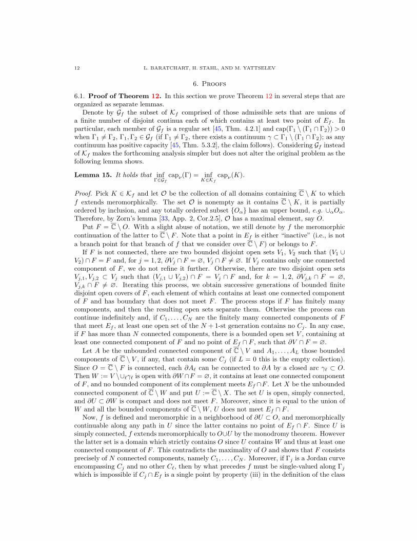
6. Proofs

6.1. Proof of Theorem 12. In this section we prove Theorem 12 in several steps that areorganized as separate lemmas.

Denote by Gf the subset of Kf comprised of those admissible sets that are unions ofa finite number of disjoint continua each of which contains at least two point of Ef . Inparticular, each member of Gf is a regular set [45, Thm. 4.2.1] and cap(Γ1 \ (Γ1 ∩ Γ2)) > 0when Γ1 6= Γ2, Γ1,Γ2 ∈ Gf (if Γ1 6= Γ2, there exists a continuum γ ⊂ Γ1 \ (Γ1 ∩ Γ2); as anycontinuum has positive capacity [45, Thm. 5.3.2], the claim follows). Considering Gf insteadof Kf makes the forthcoming analysis simpler but does not alter the original problem as thefollowing lemma shows.

Lemma 15. It holds that infΓ∈Gf

capν(Γ) = infK∈Kf

capν(K).

Proof. Pick K ∈ Kf and let O be the collection of all domains containing C \K to whichf extends meromorphically. The set O is nonempty as it contains C \ K, it is partiallyordered by inclusion, and any totally ordered subset Oα has an upper bound, e.g. ∪αOα.Therefore, by Zorn’s lemma [33, App. 2, Cor.2.5], O has a maximal element, say O.

Put F = C \ O. With a slight abuse of notation, we still denote by f the meromorphiccontinuation of the latter to C \ F . Note that a point in Ef is either “inactive” (i.e., is nota branch point for that branch of f that we consider over C \ F ) or belongs to F .

If F is not connected, there are two bounded disjoint open sets V1, V2 such that (V1 ∪V2) ∩ F = F and, for j = 1, 2, ∂Vj ∩ F = ∅, Vj ∩ F 6= ∅. If Vj contains only one connectedcomponent of F , we do not refine it further. Otherwise, there are two disjoint open setsVj,1, Vj,2 ⊂ Vj such that (Vj,1 ∪ Vj,2) ∩ F = Vj ∩ F and, for k = 1, 2, ∂Vj,k ∩ F = ∅,Vj,k ∩ F 6= ∅. Iterating this process, we obtain successive generations of bounded finitedisjoint open covers of F , each element of which contains at least one connected componentof F and has boundary that does not meet F . The process stops if F has finitely manycomponents, and then the resulting open sets separate them. Otherwise the process cancontinue indefinitely and, if C1, . . . , CN are the finitely many connected components of Fthat meet Ef , at least one open set of the N + 1-st generation contains no Cj . In any case,if F has more than N connected components, there is a bounded open set V , containing atleast one connected component of F and no point of Ef ∩ F , such that ∂V ∩ F = ∅.

Let A be the unbounded connected component of C \ V and A1, . . . , AL those boundedcomponents of C \ V , if any, that contain some Cj (if L = 0 this is the empty collection).Since O = C \ F is connected, each ∂A` can be connected to ∂A by a closed arc γ` ⊂ O.Then W := V \∪`γ` is open with ∂W ∩F = ∅, it contains at least one connected componentof F , and no bounded component of its complement meets Ef ∩F . Let X be the unboundedconnected component of C \W and put U := C \X. The set U is open, simply connected,and ∂U ⊂ ∂W is compact and does not meet F . Moreover, since it is equal to the union ofW and all the bounded components of C \W , U does not meet Ef ∩ F .

Now, f is defined and meromorphic in a neighborhood of ∂U ⊂ O, and meromorphicallycontinuable along any path in U since the latter contains no point of Ef ∩ F . Since U issimply connected, f extends meromorphically to O∪U by the monodromy theorem. Howeverthe latter set is a domain which strictly contains O since U contains W and thus at least oneconnected component of F . This contradicts the maximality of O and shows that F consistsprecisely of N connected components, namely C1, . . . , CN . Moreover, if Γj is a Jordan curveencompassing Cj and no other C`, then by what precedes f must be single-valued along Γjwhich is impossible if Cj ∩Ef is a single point by property (iii) in the definition of the class


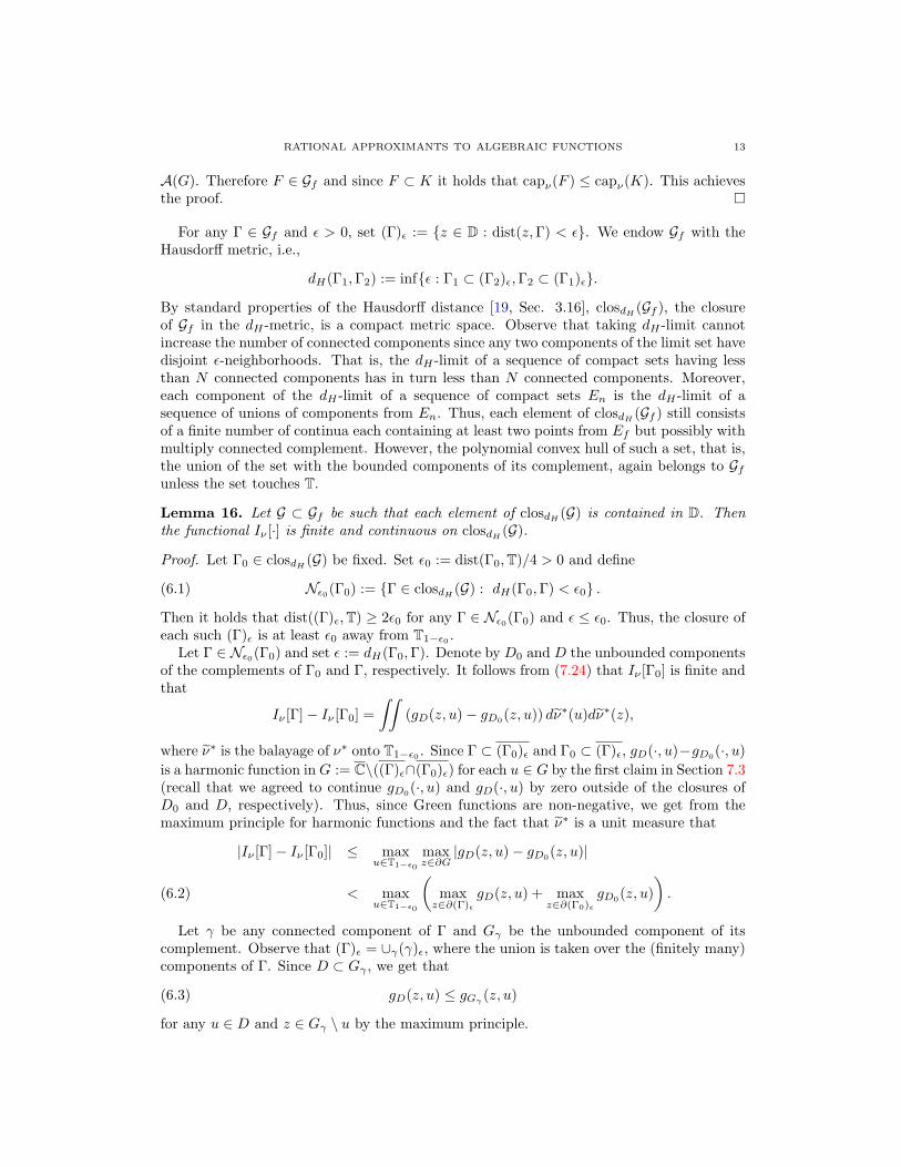
A(G). Therefore F ∈ Gf and since F ⊂ K it holds that capν(F ) ≤ capν(K). This achievesthe proof.

For any Γ ∈ Gf and ε > 0, set (Γ)ε := z ∈ D : dist(z,Γ) < ε. We endow Gf with theHausdorff metric, i.e.,

dH(Γ1,Γ2) := infε : Γ1 ⊂ (Γ2)ε,Γ2 ⊂ (Γ1)ε.

By standard properties of the Hausdorff distance [19, Sec. 3.16], closdH (Gf ), the closureof Gf in the dH -metric, is a compact metric space. Observe that taking dH -limit cannotincrease the number of connected components since any two components of the limit set havedisjoint ε-neighborhoods. That is, the dH -limit of a sequence of compact sets having lessthan N connected components has in turn less than N connected components. Moreover,each component of the dH -limit of a sequence of compact sets En is the dH -limit of asequence of unions of components from En. Thus, each element of closdH (Gf ) still consistsof a finite number of continua each containing at least two points from Ef but possibly withmultiply connected complement. However, the polynomial convex hull of such a set, that is,the union of the set with the bounded components of its complement, again belongs to Gfunless the set touches T.

Lemma 16. Let G ⊂ Gf be such that each element of closdH (G) is contained in D. Thenthe functional Iν [·] is finite and continuous on closdH (G).

Proof. Let Γ0 ∈ closdH (G) be fixed. Set ε0 := dist(Γ0,T)/4 > 0 and define

(6.1) Nε0(Γ0) := Γ ∈ closdH (G) : dH(Γ0,Γ) < ε0 .

Then it holds that dist((Γ)ε,T) ≥ 2ε0 for any Γ ∈ Nε0(Γ0) and ε ≤ ε0. Thus, the closure ofeach such (Γ)ε is at least ε0 away from T1−ε0 .

Let Γ ∈ Nε0(Γ0) and set ε := dH(Γ0,Γ). Denote by D0 and D the unbounded componentsof the complements of Γ0 and Γ, respectively. It follows from (7.24) that Iν [Γ0] is finite andthat

Iν [Γ]− Iν [Γ0] =∫∫

(gD(z, u)− gD0(z, u)) dν∗(u)dν∗(z),

where ν∗ is the balayage of ν∗ onto T1−ε0 . Since Γ ⊂ (Γ0)ε and Γ0 ⊂ (Γ)ε, gD(·, u)−gD0(·, u)is a harmonic function in G := C\((Γ)ε∩(Γ0)ε) for each u ∈ G by the first claim in Section 7.3(recall that we agreed to continue gD0(·, u) and gD(·, u) by zero outside of the closures ofD0 and D, respectively). Thus, since Green functions are non-negative, we get from themaximum principle for harmonic functions and the fact that ν∗ is a unit measure that

|Iν [Γ]− Iν [Γ0]| ≤ maxu∈T1−ε0

maxz∈∂G

|gD(z, u)− gD0(z, u)|

< maxu∈T1−ε0

(maxz∈∂(Γ)ε

gD(z, u) + maxz∈∂(Γ0)ε

gD0(z, u)).(6.2)

Let γ be any connected component of Γ and Gγ be the unbounded component of itscomplement. Observe that (Γ)ε = ∪γ(γ)ε, where the union is taken over the (finitely many)components of Γ. Since D ⊂ Gγ , we get that

(6.3) gD(z, u) ≤ gGγ (z, u)

for any u ∈ D and z ∈ Gγ \ u by the maximum principle.


Set δ :=√

2ε/cap(γ) and L to be the log(1 + δ)-level line of gGγ (·,∞). As Gγ is simplyconnected, L is a smooth Jordan curve.7 Since γ is a continuum, it is well-known thatcap(γ) ≥ diam(γ)/4 [45, Thm. 5.3.2]. Recall also that γ contains at least two points fromEf . Thus, diam(γ) is bounded from below by the minimal distance between the algebraicsingularities of f . Hence, we can assume without loss of generality that δ ≤ 1. We claim thatdist(γ, L) ≥ ε and postpone the proof of this claim until the end of this lemma. The claimimmediately implies that (γ)ε is contained in the bounded component of the complement ofL and that

(6.4) maxz∈∂(γ)ε

gGγ (z,∞) ≤ log(1 + δ) ≤ δ.

It follows from the conformal invariance of the Green function [45, Thm. 4.4.2] and canbe readily verified using the characteristic properties that gGγ (z, u) = gGuγ (1/(z − u),∞),where Guγ is the image of Gγ under the map 1/(· − u). It is also simple to compute that

(6.5) dist(γu, ∂(γ)uε ) ≤ ε

dist(u, γ)dist(u, ∂(γ)ε)≤ ε

ε20, u ∈ T1−ε0 ,

by the remark after (6.1), where γu and (γ)uε have obvious meaning. So, combining (6.5)with (6.4) applied to γu, we deduce that

(6.6) maxz∈∂(γ)ε

gGγ (z, u) = maxz∈∂(γ)uε

gGuγ (z,∞) ≤ maxz∈∂(γu)

ε/ε20

gGuγ (z,∞) ≤ δu, u ∈ T1−ε0 ,

where we put δu :=√

2ε/ε20cap(γu).As we already mentioned, cap(γ) ≥ diam(γ)/4. Hence, it holds that

(6.7) minu∈T1−ε0

cap(γu) ≥ 14

minu∈T1−ε0

maxz,w∈γ

∣∣∣∣ 1z − u

− 1w − u

∣∣∣∣ ≥ diam(γ)16

.

Gathering together (6.3), (6.6), and (6.7), we derive that

maxu∈T1−ε0

maxz∈∂(Γ)ε

gD(z, u) ≤ maxγ

4ε0

√2ε

diam(γ),

where γ ranges over all components of Γ. Recall that each component of Γ contains at leasttwo points from Ef . Thus, 1/diam(γ) is bounded above by a constant that depends onlyon f .

Arguing in a similar fashion for Γ0, we obtain from (6.2) that

|Iν [Γ]− Iν [Γ0]| ≤ const.ε0

√dH(Γ,Γ0) for any Γ ∈ Nε0(Γ0),

where const. is a constant depending only on f . This finishes the proof of the lemma grantedwe prove the claim made before (6.4).

It was claimed that for a continuum γ and the log(1 + δ)-level line L of gGγ (·,∞), δ ≤ 1,it holds that

(6.8) dist(γ, L) ≥ δ2cap(γ)2

,

where Gγ is the unbounded component of the complement of γ. Inequality (6.8) was provedin [42, Lem. 1], however, this work was never published and the authors felt compelled toreproduce this lemma here.

7By conformal invariance of Green functions it is enough to check it for Gγ = O in which case it is

obvious.


Let Φ be a conformal map of O onto Gγ , Φ(∞) =∞. It is well-known that |Φ(z)z−1| →cap(γ) as z → ∞ and that gGγ (·,∞) = log |Φ−1|, where Φ−1 is the inverse of Φ (that is, aconformal map of Gγ onto O, Φ−1(∞) =∞). Then it follows from [24, Thm. IV.2.1] that

(6.9) |Φ′(z)| ≥ cap(γ)(

1− 1|z|2

), z ∈ O.

Let z1 ∈ γ and z2 ∈ L be such that dist(γ, L) = |z1 − z2|. Denote by [z1, z2] the segmentjoining z1 and z2. Observe that Φ−1 maps the annular domain bounded by γ and L ontothe annulus z : 1 < |z| < 1 + δ. Denote by S the intersection of Φ−1((z1, z2)) with thisannulus. Clearly, the angular projection of S onto the real line is equal to (1, 1 + δ). Then

dist(γ, L) =∫

(z1,z2)

|dz| =∫

Φ−1((z1,z2))

|Φ′(z)||dz| ≥ cap(γ)∫

Φ−1((z1,z2))

(1− 1|z|2

)|dz|

≥ cap(γ)∫S

(1− 1|z|2

)|dz| ≥ cap(γ)

∫(1,1+δ)

(1− 1|z|2

)|dz| = δ2cap(γ)

1 + δ,

where we used (6.9). This proves (6.8) since it is assumed that δ ≤ 1.

Set prρ(·) to be the radial projection onto Dρ, i.e., prρ(z) = z if |z| ≤ ρ and prρ(z) = ρz/|z|if ρ < |z| < ∞. Put further prρ(K) := prρ(z) : z ∈ K. In the following lemma we showthat prρ can only increase the value of Iν [·].

Lemma 17. Let Γ ∈ Gf and ρ ∈ [r, 1), r = maxz∈Ef |z|. Then prρ(Γ) ∈ Gf andcapν(prρ(Γ)) ≤ capν(Γ).

Proof. As Ef ⊂ Dr, f naturally extends along any ray tξ, ξ ∈ T, t ∈ (r,∞). Thus, the germf has a representative which is single-valued and meromorphic outside of prρ(Γ). It is alsotrue that prρ is a continuous map on C and therefore cannot disconnect the components ofΓ although it may merge some of them. Thus, prρ(Γ) ∈ Gf .

Set w = expUν and

δwm(Γ) := supz1,...,zm∈Γ

∏1≤j<i≤m

|zi − zj |w(zi)w(zj)

2/m(m−1)

.

It is known [47, Thm. III.1.3] that δwm(Γ) → capν(Γ) as m → ∞. Thus, it is enough toobtain that δwm(prρ(Γ)) ≤ δwm(Γ) holds for any m. In turn, it is sufficient to show that

(6.10) |prρ(z1)− prρ(z2)|w(prρ(z1))w(prρ(z2)) ≤ |z1 − z2|w(z1)w(z2)

for any z1, z2 ∈ D.Assume for the moment that ν = δu for some u ∈ D, i.e., w(z) = 1/|1 − zu|. It can

be readily seen that it is enough to consider only two cases: |z1| ≤ ρ, |z2| = x > ρ and|z1| = |z2| = x > ρ. In the former situation, (6.10) will follow upon showing that

l1(x) :=x2 + |z1|2 − 2x|z1| cosφ1 + x2|u|2 − 2x|u| cosψ

is an increasing function on (|z1|, 1/|u|) for any choice of φ and ψ. Since

l′1(x) = 2x(1− |u|2|z1|2)− |z1| cosφ(1− x2|u|2)− |u| cosψ(x2 − |z1|2)

(1 + x2|u|2 − 2x|u| cosψ)2

> 2(1− |u||z1|)(1− x|u|)(x− |z1|)

(1 + x|u|)4> 0,


l1 is indeed strictly increasing on (|z1|, 1/|u|). In the latter case, (6.10) is equivalent toshowing that

l2(x) := (1/x+ x|u|2 − 2|u| cosφ)(1/x+ x|u|2 − 2|u| cosψ)

is a decreasing function on (ρ, 1/|u|) for any choice of φ and ψ. This is true since

l′2(x) = 2(|u|2 − 1/x2)(1/x+ x|u|2 − |u|(cosφ+ cosψ)) < 0.

Thus, we verified (6.10) for ν = δu.In the general case it holds that

|z1 − z2|w(z1)w(z2) = exp∫

log|z1 − z2|

|1− z1u||1− z2u|dν(u)

.

As the kernel on the right-hand side of the equality above gets smaller when zj is replacedby prρ(zj), j = 1, 2, by what precedes, the validity of (6.10) follows.

Combining Lemmas 15–17, we obtain the existence of minimal sets.

Lemma 18. A minimal set Γν exists and is contained in Dr, r = max|z| : z ∈ Ef.

Proof. By Lemma 15, it is enough to consider only the sets in Gf . Let Γn ⊂ Gf be amaximizing sequence for Iν [·] (minimizing sequence for the ν-capacity), that is, Iν [Γn] tendsto supΓ∈Gf Iν [Γ] as n → ∞. Then it follows from Lemma 17 that prr(Γn) is anothermaximizing sequence for Iν [·] in Gf , and prr(Γn) ∈ Gr := Γ ∈ Gf : Γ ⊆ Dr. AsclosdH (Gr) is a compact metric space, there exists at least one limit point of prr(Γn) inclosdH (Gr), say Γ0, and Γ0 ⊂ Dr. Since Iν [·] is continuous on closdH (Gr) by Lemma 16,Iν [Γ0] = supΓ∈Gf Iν [Γ]. Finally, as the polynomial convex hull of Γ0, say Γ′0, belongs to Gfand since Iν [Γ0] = Iν [Γ′0] (see Section 7.2.4), we may put Γν = Γ′0.

To continue with our analysis we need the following theorem [32, Thm. 3.1]. It describesthe continuum of minimal condenser capacity connecting finitely many given points as aunion of closures of the non-closed negative critical trajectories of a quadratic differential.Recall that a negative trajectory of the quadratic differential q(z)dz2 is a maximally con-tinued arc along which q(z)dz2 < 0; the trajectory is called critical if it ends at a zero or apole of q(z)[32, 43].

Theorem K. Let A = a1, . . . , am ⊂ D be a set of m ≥ 2 distinct points. Then thereuniquely exists a continuum K0, A ⊂ K0 ⊂ D, such that

cap(K0,T) ≤ cap(K,T)

for any other continuum with A ⊂ K ⊂ D. Moreover, there exist m−2 points b1, . . . , bm−2 ∈D such that K0 is the union of the closures of the non-closed negative critical trajectories ofthe quadratic differential

q(z)dz2, q(z) :=(z − b1) · . . . · (z − bm−2)(1− b1z) · . . . · (1− bm−2z)

(z − a1) · . . . · (z − am)(1− a1z) · . . . · (1− amz),

contained in D. There exists only finitely many such trajectories. Furthermore, the equilib-

rium potential Vω(K0,T)

D satisfies(

2∂zVω(K0,T)

D (z))2

= q(z), z ∈ D.

The last equation in Theorem K should be understood as follows. The left-hand side ofthis equality is defined in D\K0 and represents a holomorphic function there, which coincideswith q on its domain of definition. As K0 has no interior because critical trajectories areanalytic arcs with limiting tangents at their endpoints [43], the equality on the whole set D


is obtained by continuity. Note also that D\K0 is connected by unicity claimed in Theorem6.1, for the polynomial convex hull of K0 has the same Green capacity as K0 (cf. section7.1.3). Moreover, it follows from the local theory of quadratic differentials that each bj isthe endpoint of at least three arcs of K0 (because bj is a zero of q(z)) and that each aj isthe endpoint of exactly one arc of K0 (because aj is a simple pole of q(z)).

Having Theorem K at hand, we are ready to describe the structure of a minimal set Γν .

Lemma 19. A minimal set Γν is symmetric (Definition 10) with respect to ν∗.

Proof. Let ν∗ be the balayage of ν∗ onto Tρ with ρ < 1 but large enough to contain Γν inthe interior of Dρ. Let γ be any of the continua constituting Γν . Clearly V := V eν∗

Dν, where

Dν = C \ Γν , is harmonic in Dν \ Tρ and extends continuously to the zero function on Γνsince Γν is a regular set. Moreover, by Sard’s theorem on regular values [27, Sec. 1.7] thereexists δ > 0 arbitrarily small such that Ω, the component of z : V (z) < δ containingγ, is itself contained in Dρ and its boundary is an analytic Jordan curve, say L. Let φ bea conformal map of Ω onto D. Set γ := φ−1(K), where K is the continuum of minimalcondenser capacity8 for φ(Ef ∩ γ). Our immediate goal is to show that γ = γ.

Assume to the contrary that γ 6= γ, i.e., φ(γ) =: K 6= K, and therefore

(6.11) cap(K,T) < cap(K,T).

Set

(6.12) V :=

δcap(K,T)

[Vω(T,fK)

C\ eK φ], z ∈ Ω,

V, z /∈ Ω,

where ω(T, eK) is the Green equilibrium distribution on T relative to C \ K. The functions V

and V are continuous in Ω and equal to δ on L. Furthermore, they are harmonic in Ω \ γand Ω \ γ and equal to zero on γ and γ, respectively. Then it follows from Lemma 24 andthe conformal invariance of the condenser capacity (7.7) that

(6.13)1

2π

∫L

∂V

∂nds = −δcap(K,T) and

12π

∫L

∂V

∂nds = −δcap(K,T),

where ∂/∂n stands for the partial derivative with respect to the inner normal on L. (InLemma 24, L should be contained within the domain of harmonicity of V and V . As Vand V are constant on L, they can be harmonically continued across by reflection. Thus,Lemma 24 does apply.) Moreover, V − V eν∗eD is a continuous function on C that is harmonic

in D \L by the first claim in Section 7.3, where D := (Dν ∪ γ) \ γ, and is identically zero onΓ := C \ D. Thus, we can apply Lemma 23 with V − V eν∗eD and D (smoothness properties of

V − V eν∗eD follow from the fact that V can be harmonically continued across L), which statesthat

(6.14) V = V eν∗−σeD , dσ :=1

2π∂(V − V )

∂nds,

where σ is a finite signed measure supported on L (observe that the outer and inner normalderivatives of V eν∗eD on L are opposite to each other as V eν∗eD is harmonic across L and thereforethey do not contribute to the density of σ; due to the same reasoning the outer normal

8In other words, if we put φ(Ef ∩ γ) = p1, . . . , pm and g(z) := 1/ mpQ

(z − pj), then eK is the set of

minimal condenser capacity for g as defined in Definition 2.


derivative of V is equal to minus the inner normal derivative of V by (6.12)). Hence, onecan easily deduce from (6.13) and (6.11) that

(6.15) σ(L) = δ(

cap(K,T)− cap(K,T))> 0.

Since the components of Γν and Γ contain exactly the same branch points of f and Γ hasconnected complement (for Dν is connected and so is C \ γ because D \ K is connected), itfollows that Γ ∈ Gf by the monodromy theorem. Moreover, we obtain from (7.24), (6.12),and (6.14) that

Iν [Γ]− Iν [Γν ] = I eD[ν∗]− IDν [ν∗] =∫ (

V eν∗eD − V)dν∗ =

∫V σeDdν∗

since supp(ν∗)∩Ω = ∅. Further, applying the Fubini-Tonelli theorem and using (6.14) oncemore, we get that

Iν [Γ]− Iν [Γν ] =∫V eν∗eD dσ =

∫V dσ + I eD[σ] = δσ(L) + I eD[σ] > 0

by (6.15) and since the Green energy of a signed compactly supported measure of finite Greenenergy is positive by [47, Thm. II.5.6]. However, the last inequality clearly contradicts thefact that Iν [Γν ] is maximal among all sets in Gf and therefore γ = γ. Hence, K = K = φ(γ)and V = V .

Observe now that by Theorem K stated just before this lemma and the remarks thereafter,the set K consists of a finite number of open analytic arcs and their endpoints. These fallinto two classes a1, . . . , am and b1, . . . , bm−2, members of the first class being endpoints ofexactly one arc and members of the second class being endpoints of at least three arcs. Thus,the same is true for γ. Moreover, the jump of f across any open arc C ⊂ γ cannot vanish,otherwise excising out this arc would leave us with an admissible compact set Γ′ ⊂ Γν ofstrictly smaller ν-capacity since ωΓν ,−Uν (C) > 0 by (7.23) and the properties of balayage atregular points (see Section 7.2.4). Hence Γν is a smooth cut (Definition 3). Finally, we havethat

∂V

∂n±γ= δcap(φ(γ),T)

(∂

∂n±KVω(T,K)

C\K

)|φ′|

by (6.12) and the conformality of φ, where ∂/∂n±γ and ∂/∂n±K are the partial derivativeswith respect to the one-sided normals at the smooth points of γ and K, respectively. Thus,it holds that

∂V

∂n−γ=

∂V

∂n+γ

on the open arcs constituting γ since the corresponding property holds for V ω(T,K)

C\K by (2.5).As γ was arbitrary continuum from Γν , we see that all the requirements of Definition 10 arefulfilled.

To finish the proof of Theorem 12, it only remains to show uniqueness of Γν , which isachieved through the following lemma:

Lemma 20. Γν is uniquely characterized as a compact set symmetric with respect to ν∗.

Proof. Let Γs ∈ Gf be symmetric with respect to ν∗ and Γν be any set of minimal capacityfor Problem (f, ν). Such a set exists by Lemma 18 and it is symmetric by Lemma 19.Suppose to the contrary that Γs 6= Γν , that is,

(6.16) Γs ∩ (C \ Γν) 6= ∅


(Γs cannot be a strict subset of Γν for it would have strictly smaller ν-capacity as pointedout in the proof of Lemma 19). We want to show that (6.16) leads to

(6.17) Iν [Γs]− Iν [Γν ] > 0.

Clearly, (6.17) is impossible by the very definition of Γν and therefore the lemma will beproven.

By the very definition of symmetry (Definition 10), Γν and Γs are smooth cuts for f . Inparticular, C \ Γν , C \ Γs are connected and we have a decomposition of the form

Γs = Es0 ∪ Es1 ∪⋃γsj and Γν = Eν0 ∪ Eν1 ∪

⋃γνj ,

where Es0 , Eν0 ⊆ Ef , γνj , γ

sj are open analytic arcs, and each element of Es0 , E

ν0 is an endpoint

of exactly one arc from⋃γsj ,

⋃γνj while Es1 , E

ν1 are finite sets of points each elements of

which serving as an endpoint for at least three arcs from⋃γsj ,⋃γνj , respectively. Moreover,

the continuations of f from infinity that are meromorphic outside of Γs and Γν , say fs andfν , are such that the jumps f+

s − f−s and f+ν − f−ν do not vanish on any subset with a limit

point of⋃γsj and

⋃γνj , respectively. Note that Γs ∩ Γν 6= ∅ otherwise C \ (Γν ∪ Γs) would

be connected, so f could be continued analytically over (C \Γν)∪ (C \Γs) = C and it wouldbe identically zero by our normalization.

Write Γs = Γ1s ∪Γ2

s and Γν = Γ1ν ∪Γ2

ν , where Γks (resp. Γkν) are compact disjoint sets suchthat each connected component of Γ1

s (resp. Γ1ν) has nonempty intersection with Γν (resp.

Γs) while Γ2s ∩ Γν = Γ2

ν ∩ Γs = ∅.Now, put, for brevity, Dν := C\Γν and Ds := C\Γs. Denote further by Ω the unbounded

component of Dν ∩Ds. Then

(6.18) Ω ∩ Es0 ∩ Γ1s = Ω ∩ Eν0 ∩ Γ1

ν .

Indeed, assume that there exists e ∈ (Ω∩Es0∩Γ1s)\(Eν0∩Γ1

ν) and let γse be the arc in the union⋃γsj that has e as one of the endpoints. By our assumption there is an open disk W centered

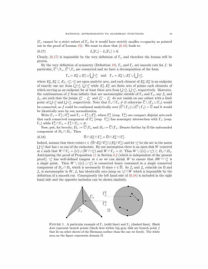
at e such that W ∩ Γs = e ∪ (W ∩ γse) and W ∩ Γν = ∅. Thus W \ (e ∪ γse) ⊂ Dν ∩Ds.Anticipating the proof of Proposition 11 in Section 6.2 (which is independent of the presentproof), γse has well-defined tangent at e so we can shrink W to ensure that ∂W ∩ γse isa single point. Then W \ (e ∪ γse) is connected hence contained in a single connectedcomponent of Dν ∩Ds which is necessarily Ω since e ∈ Ω. As fs and fν coincide on Ω andfν is meromorphic in W , fs has identically zero jump on γse ∩W which is impossible by thedefinition of a smooth cut. Consequently the left hand side of (6.18) is included in the righthand side and the opposite inclusion can be shown similarly.

Ω

Γ2s

Γ3s

Γs

Γν

Figure 1. A particular example of Γs (solid lines) and Γν (dashed lines). Blackdots represent branch points (black dots within big gray disk are branch point fthat lie on other sheets of the Riemann surface than the one we fixed). The whitearea on the figure represents domain Ω.


Next, observe that

(6.19) Γ2s ∩ Ω = ∅.

Indeed, since ∂Ω ⊂ Γs∪Γν and Γ2s, Γ1

s∪Γν are disjoint compact sets, a connected componentof ∂Ω that meets Γ2

s is contained in it. If z ∈ Γ2s ∩ ∂Ω lies on γsj , then by analyticity of the

latter each sufficiently small disk Dz centered at z is cut out by γsj ∩Dz into two connectedcomponents included in Dν ∩ Ds, and of necessity one of them is contained in Ω. Henceγsj ∩Dz is contained in ∂Ω, and in turn so does the entire arc γsj by connectedness. Henceevery component of Γ2

s ∩ ∂Ω consists of a union of arcs γsj connecting at their endpoints.Because Γ2

s has no loop, one of them has an endpoint z1 ∈ Es0 ∪ Es1 belonging to no otherarc. If z1 ∈ Es0 , reasoning as we did to prove (6.18) leads to the absurd conclusion that fshas zero jump across the initial arc. If z1 ∈ Es1 , anticipating the proof of Proposition 11 onceagain, each sufficiently small disk Dz1 centered at z1 is cut out by Γ2

s ∩Dz1 into curvilinearsectors included in Dν ∩Ds, and of necessity one of them is contained in Ω whence at leasttwo adjacent arcs γsj emanating from z1 are included in ∂Ω. This contradicts the fact thatz1 belongs to exactly one arc of the hypothesized component of Γ2

s ∩ ∂Ω, and proves (6.19).Finally, set

Γ3s :=

[Γ1s \ (∂Ω \ Es1)

]∩Dν and Γ4

s :=[Γ1s ∩⋃γsj

]∩ ∂Ω ∩Dν .

Clearly

(6.20)(Γ3s \ Es1

)∩ Ω = ∅.

Moreover, observing that any two arcs γsj , γνk either coincide or meet in a (possibly empty)discrete set and arguing as we did to prove (6.19), we see that

[Γ1s ∩⋃γsj]∩ ∂Ω consists

of subarcs of arcs γsj whose endpoints either belong to some intersection γsj ∩ γνk (in whichcase they contain this endpoint) or else lie in Es0 ∪ Es1 (in which case they do not containthis endpoint). Thus Γ4

s is comprised of open analytic arcs γs` contained in ∂Ω ∩⋃γsj and

disjoint from Γν . Hence for any z ∈ Γ4s, say z ∈ γs` , and any disk Dz centered at z of small

enough radius it holds that Dz ∩ ∂Ω = Dz ∩ γs` and that Dz \ γs` has exactly two connectedcomponents:

(6.21) Dz ∩ Ω 6= ∅ and Dz ∩(C \ Ω

)6= ∅

for if z ∈ γs` was such that Dz \ γs` ⊂ Ω, the jump of fs across γs` would be zero as the jumpof fν is zero there and fs = fν in Ω (see Figure 1).

As usual, denote by ν∗ the balayage of ν∗ onto Tρ with ρ ∈ (r, 1) but large enough sothat Γs and Γν are contained in the interior of Dρ (see Lemma 18 for the definition of r).Then, according to (7.24) and (7.39), it holds that

(6.22) Iν [Γs]− Iν [Γν ] = IDs [ν∗]− IDν [ν∗] = DDs(Vs)−DDν (Vν),

where Vs := V eν∗Ds

and Vν := V eν∗Dν

. Indeed, as ν∗ has finite energy (see Section 7.2.3), theDirichlet integrals of Vs and Vν in the considered domains (see Section 7.4) are well-definedby Proposition 11, which is proven later but independently of the results in this section.

Set D := Dν \ (Γ2s ∪ Γ3

s). Since[Γ1s \ (∂Ω \ Es1)

]consists of piecewise smooth arcs in Γ1

s

whose endpoints either belong to this arc (if they lie in Es1), or to Es0 ∩ Γ1s (hence also to

Γν by (6.18)), or else to some intersection γsj ∩ γνk (in which case they belong to Γν again),we see that D is an open set. As Vν is harmonic across Γ2

s ∪ Γ3s and Vs is harmonic across

Γν \ Γs, we get from (7.38) that

(6.23) DDν (Vν) = DD(Vν) and DDs(Vs) = DD\Γ4s(Vs)


since Ds \ Γν = Dν \ Γs = D \ Γ4s, by inspection on using (6.18).

Now, recall that Γs has no interior and Vs ≡ 0 on Γs, that is, Vs is defined in the wholecomplex plane. So, we can define a function on C by putting

(6.24) V :=

Vs, in Ω,−Vs, otherwise.

We claim that V is superharmonic in D and harmonic in D \ Tρ. Indeed, it is clearlyharmonic in D \ (Γ4

s ∪Tρ) = (Ds ∩Dν) \Tρand superharmonic in a neighborhood of Tρ ⊂ Ωwhere its weak Laplacian is −2πν∗ which is a negative measure. Moreover, Γ4

s is a collectionof open analytic arcs such that ∂Vs/∂n+ = ∂Vs/∂n− by the symmetry of Γs, where n±

are the two-sided normal on each subarc of Γ4s. The equality of the normals means that

Vs can be continued harmonically across each subarc of Γ4s by −Vs. Hence, (6.21) and the

definition of V yield that it is harmonic across Γ4s thereby proving the claim. Thus, using

(7.41) (applied with D′ = Ω) and (7.38), we obtain

(6.25) DD\Γ4s(Vs) = DD\Γ4

s(V ) = DD(V )

hence combining (6.22), (6.23), and (6.25), we see that

(6.26) Iν [Γs]− Iν [Γν ] = DD(V )−DD(Vν).

By the first claim in Section 7.3, it holds that h := V − Vν is harmonic in D. Observethat h is not a constant function, for it tends to zero at each point of Γs ∩Γν ⊂ ∂D whereasit tends to a strictly negative value at each point of Γs ∩ Dν ⊂ D which is nonempty by(6.16). Then

(6.27) DD(V ) = DD(Vν) + DD(h) + 2DD(Vν , h).

Now, Vν ≡ 0 on Γν and it is harmonic across Γ2s ∪ Γ3

s, hence

∂h

∂n++

∂h

∂n−=

∂V

∂n++

∂V

∂n−on Γ2

s ∪ Γ3s.

Consequently, we get from (7.35), since V = −Vs in the neighborhood of Γ2s ∪ Γ3

s by (6.19)and (6.20), that

(6.28) DD(Vν , h) = −∫

Γ2s∪Γ3

s

Vν

(∂V

∂n++

∂V

∂n−

)ds

2π=∫

Γ2s∪Γ3

s

Vν

(∂Vs∂n+

+∂Vs∂n−

)ds

2π≥ 0

because Vν is nonnegative while ∂Vs/∂n+, ∂Vs/∂n− are also nonnegative on Γ2

s ∪ Γ3s as

Vs ≥ 0 vanishes there. Altogether, we obtain from (6.26), (6.27), and (6.28) that

Iν [Γs]− Iν [Γν ] ≥ DD(h) > 0

by (7.40) and since h = V −Vν is a non-constant harmonic function in D. This shows (6.17)and finishes the proof of the lemma.

6.2. Proof of Proposition 11. It is well known that Hω,Γ is holomorphic in the domainof harmonicity of V ωC\Γ, that is, in C\(Γ∪supp(ω)). It is also clear that H±ω,Γ exist smoothlyon each γj since V ωC\Γ can be harmonically continued across each side of γj .

Denote by n±t the one-sided unit normals at t ∈⋃γj and by τt the unit tangent pointing in

the positive direction. Let further n±(t) be the unimodular complex numbers corresponding


to vectors n±t . Then the complex number corresponding to τt is ∓in±(t) and it can bereadily verified that

∂V ωC\Γ

∂n±t= 2Re

(n±(t)H±ω,Γ(t)

)and

∂(V ωC\Γ

)±∂τt

= ∓2Im(n±(t)H±ω,Γ(t)

).

As(V ωC\Γ

)±≡ 0 on Γ, the tangential derivatives above are identically zero, therefore n±H±ω,Γ

is real on Γ. Moreover since n+ = −n− and by the symmetry property (4.3), it holds thatH+ω,Γ = −H−ω,Γ on

⋃γj . Hence, H2

ω,Γ is holomorphic in C\(E0∪E1∪supp(ω)). Since E0∪E1

consists of isolated points around which H2ω,Γ is holomorphic each e ∈ E0 ∪ E1 is either a

pole, a removable singularity, or an essential one. As Hω,Γ is holomorphic on a two-sheetedRiemann surface above the point, it cannot have an essential singularity since its primitivehas bounded real part ±V ωC\Γ. Now, by repeating the arguments in [43, Sec. 8.2], we deduce

that (z− e)je−2H2ω,Γ(z) is holomorphic and non-vanishing in some neighborhood of e where

je is the number of arcs γj having e as an endpoint, that the tangents at e to these arcsexist, and that they are equiangular if je > 1.

6.3. Proof of Theorem 14. The following theorem [25, Thm. 3] and its proof are essen-tial in establishing Theorem 14. Before stating this result, we remind the reader that apolynomial v is said to by spherically normalized if it has the form

(6.29) v(z) =∏

v(e)=0, |e|≤1

(z − e)∏

v(e)=0, |e|>1

(1− z/e).

We also recall from [25] the notions of a tame set and a tame point of a set. A point zbelonging to a compact set Γ is called tame, if there is a disk centered at z whose intersectionwith Γ is an analytic arc. A compact set Γ is called tame, if Γ is non-polar and quasi-everypoint of Γ is tame.

A tame compact set Γ is said to have the S-property in the field ψ, assumed to beharmonic in some neighborhood of Γ, if supp(ωΓ,ψ) forms a tame set as well, every tamepoint of supp(ωΓ,ψ) is also a tame point of Γ, and the equality in (4.4) holds at each tamepoint of supp(ωΓ,ψ).

Whenever the tame compact set Γ has connected complement in a simply connectedregion G ⊃ Γ and g is holomorphic in G \ Γ, we write

∮Γg(t) dt for the contour integral of g

over some (hence any) system of curves encompassing Γ once in G in the positive direction.Likewise, the Cauchy integral

∮Γg(t)/(z − t) dt can be defined at any z ∈ C \ Γ by choosing

the previous system of curves in such a way that it separates z from Γ.If g has limits from each side at tame points of Γ, and if these limits are integrable

with respect to linear measure on Γ, then the previous integrals may well be rewritten asintegrals on Γ with g replaced by its jump across Γ. However, this is not what is meant bythe notation

∮Γ.

Theorem GR. Let G ⊂ D be a simply connected domain and Γ ⊂ G be a tame compactset with connected complement. Let also g be holomorphic in G \ Γ and have continuouslimits on Γ from each side in the neighborhood of every tame point, whose jump across Γ isnon-vanishing q.e. Further, let Ψn be a sequence of functions that satisfy:

(1) Ψn is holomorphic in G and − 12n log |Ψn| → ψ locally uniformly there, where ψ is

harmonic in G;(2) Γ possesses the S-property in the field ψ (see (4.4)).


Then, if the polynomials qn, deg(qn) ≤ n, satisfy the orthogonality relations9

(6.30)∮

Γ

qn(t)ln−1(t)Ψn(t)g(t)dt = 0, for any ln−1 ∈ Pn−1,

then µn∗→ ωΓ,ψ, where µn is the normalized counting measure of zeros of qn. Moreover, if

the polynomials qn are spherically normalized, it holds that

(6.31) |An(z)|1/2n cap→ exp−c(ψ; Γ) in C \ Γ,

where c(ψ; Γ) is the modified Robin constant (Section 7.1.2), and

(6.32) An(z) :=∮

Γ

q2n(t)

(Ψng)(t)dtz − t

=qn(z)ln(z)

∮Γ

(lnqn)(t)(Ψng)(t)dtz − t

,

where ln can be any10 nonzero polynomial of degree at most n.

Proof of Theorem 14. Let En be the sets constituting the interpolation scheme E . Set Ψn tobe the reciprocal of the spherically normalized polynomial with zeros at the finite elementsof En, i.e., Ψn = 1/vn, where vn is the spherical renormalization of vn (see Definition 13and (6.29)). Then the functions Ψn are holomorphic and non-vanishing in C \ supp(E) (inparticular, in D), 1

2n log |Ψn|cap→ Uν in C \ supp(ν∗) by Lemma 21, and this convergence is

locally uniform in D by definition of the asymptotic distribution and since log 1/|z − t| iscontinuous on a neighborhood of supp(E) for fixed z ∈ D. As Uν is harmonic in D, require-ment (1) of Theorem GR is fulfilled with G = D and ψ = −Uν . Further, it follows fromTheorem 12 that Γν is a symmetric set. In particular it is a smooth cut, hence it is tamewith tame points ∪jγj . Moreover, since Γν is regular, we have that supp(ωΓ,ψ) = Γν by(7.18) and properties of balayage (Section 7.2.2). Thus, by the remark after Definition 10,symmetry implies that Γν possesses the S-property in the field −Uν and therefore require-ment (2) of Theorem GR is also fulfilled. Let now Q, deg(Q) =: m, be a fixed polynomialsuch that the only singularities of Qf in D belong to Ef . Then Qf is holomorphic andsingle-valued in D\Γν , it extends continuously from each side on ∪γj , and has a jump therewhich is continuous and non-vanishing except possibly at countably many points. All therequirement of Theorem GR are then fulfilled with g = Qf .

Let L ⊂ D be a smooth Jordan curve that separates Γν and the poles of f (if any) from E .Denote by qn the spherically normalized denominators of the multipoint Pade approximantsto f associated with E . It is a standard consequence of Definition 13 (see e.g. [25, sec.1.5.1]) that

(6.33)∫L

zjqn(z)Ψn(z)f(z)dz = 0, j ∈ 0, . . . , n− 1.

Clearly, relations (6.33) imply that

(6.34)∮

Γν

(lqnΨnfQ)(t)dt = 0, deg(l) < n−m.

Equations (6.34) differ from (6.30) only in the reduction of the degree of polynomials l bya constant m. However, to derive the first conclusion of Theorem GR, namely that µn

∗→ωΓ,ψ, orthogonality relations (6.30) are used solely when applied to a specially constructedsequence ln such that ln = ln,1ln,2, where deg(ln,1) ≤ nθ, θ < 1, and deg(ln,2) = o(n) asn→∞ (see the proof of [25, Thm. 3] in between equations (27) and (28)). Thus, the proof

9Note that the orthogonality in (6.30) is non-Hermitian, that is, no conjugation is involved.10The fact that we can pick an arbitrary polynomial ln for this integral representation of An is a simple

consequence of orthogonality relations (6.30).


is still applicable in our situation, to the effect that the normalized counting measures ofthe zeros of qn converge weak∗ to ν∗ = ωΓν ,−Uν , see (7.23).

For each n ∈ N, let qn,m, deg(qn,m) = n − m, be a divisor of qn. Observe that thepolynomials qn,m have exactly the same asymptotic zero distribution in the weak∗ sense asthe polynomials qn. Put

(6.35) An,m(z) :=∮

(qn,mqn)(t)(ΨnfQ)(t)dt

z − t, z ∈ Dν .

Due to orthogonality relations (6.34), An,m can be equivalently rewritten as

(6.36) An,m(z) :=qn,m(z)ln−m(z)

∮(ln−mqn)(t)

(ΨnfQ)(t)dtz − t

, z ∈ Dν ,

where ln−m is an arbitrary polynomial of degree at most n−m. Formulae (6.35) and (6.36)differ from (6.32) in the same manner as orthogonality relations (6.34) differ from those in(6.30). Examination of the proof of [25, Thm. 3] (see the discussion there between equations(33) and (37)) shows that limit (6.31) is proved using expression (6.32) for An with a choiceof polynomials ln that satisfy some set of asymptotic requirements and can be chosen tohave the degree n−m. Hence it still holds that

(6.37) |An,m(z)|1/2n cap→ exp −c(−Uν ; Γν) in Dν .

Finally, using the Hermite interpolation formula like in [52, Lem. 6.1.2], the error ofapproximation has the following representation

(6.38) (f −Πn)(z) =An,m(z)

(qn,mqnQΨn)(z), z ∈ Dν .

From Lemma 21 we know that log(1/|qn|)/ncap→ V cν∗

∗ = V cν∗ in Dν , since ordinary andspherically normalized potentials coincide for measures supported in D. This fact togetherwith (6.37) and (6.38) easily yield that

|f −Πn|1/2ncap→ exp

−c(−Uν ; Γν) + V bν∗ − Uν in Dν \ supp(ν∗).

Therefore, (5.1) follows from (7.20) and the fact that Uν = V ν∗

∗ by the remark at thebeginning of Section 7.2.4.

6.4. Proof of Theorem 4, Theorem 7, Corollary 8, Theorem 6, and Theorem 5.

Proof of Theorem 4. Let Γ ∈ Kf (G) be a smooth cut for f that satisfies (2.5) and Θ be aconformal map of D onto G. Set K := Θ−1(Γ). Then we get from the conformal invarianceof the condenser capacity (see (7.7)) and the maximum principle for harmonic functions that

cap(Γ, T ) = cap(K,T) and Vω(K,T)

C\K = Vω(Γ,T )

C\Γ Θ in D.

As Θ is conformal in D, it can be readily verified that V ω(K,T)

C\K satisfies (2.5) as well (naturally,

on K). Univalence of Θ also implies that the continuation properties of (f Θ)(Θ′)1/2 in Dare exactly the same as those of f in G. Moreover, this is also true for fΘ, the orthogonalprojection of (f Θ)(Θ′)1/2 from L2 onto H2

0 (see Section 3). Indeed, fΘ is holomorphicin O by its very definition and can be continued analytically across T by (f Θ)(Θ′)1/2

minus the orthogonal projection of the latter from L2 onto H2, which is holomorphic in Dby definition. Thus, fΘ ∈ A(D) and Γ ∈ Kf (G) if and only if K ∈ KfΘ . Therefore, it isenough to consider only the case G = D.


Let Γ ∈ Kf be a smooth cut for f that satisfies (2.5) and K be the set of minimal condensercapacity (cf. Theorem 2). We must prove that Γ = K. Set, for brevity, DΓ := C \ Γ,VΓ := V

ω(T,Γ)

DΓ, DK := C \ K, VK := V

ω(T,K)

DK, and Ω to be the unbounded component of

DK ∩ DΓ. Let also fDΓ and fDK indicate the meromorphic branches of f in DΓ and DK,respectively. Arguing as we did to prove (6.19), we see that no connected component of ∂Ωcan lie entirely in Γ \ K (resp. K \ Γ) otherwise the jump of fDΓ (resp. fDK) across somesubarc of Γ (resp. K) would vanish. Hence by connectedness

(6.39) Γ ∩K ∩ ∂Ω 6= ∅.

First, we deal with the special situation where ω(T,K) = ω(T,Γ). Then VΓ − VK is harmonicin Ω by the first claim in Section 7.3. As both potentials are constant in O ⊂ Ω, we getthat VΓ = VK + const. in Ω. Since K and Γ are regular sets, potentials VΓ and VK extendcontinuously to ∂Ω and vanish at ∂Ω ∩ Γ ∩K which is non-empty by (6.39). Thus, equalityof the equilibrium measures means that VΓ ≡ VK in Ω. However, because VΓ (resp. VK)vanishes precisely on Γ (resp. K), this is possible only if ∂Ω ⊂ Γ ∩K. Taking complementsin C, we conclude that DΓ ∪ DK, which is connected and contains ∞, does not meet ∂Ω.Therefore DΓ ∪DK ⊂ Ω ⊂ DΓ ∩DK, hence DΓ = DK thus Γ = K, as desired.

In the rest of the proof we assume for a contradiction that Γ 6= K. Then ω(T,K) 6= ω(T,Γ)

in view of what precedes, and therefore

(6.40) DDK(VK) = IDK

[ω(T,K)

]< IDK

[ω(T,Γ)

]= DDK(V ω(T,Γ)

DK)

by (7.39) and since the Green equilibrium measure is the unique minimizer of the Greenenergy.

The argument now follows the lines of the proof of Lemma 20. Namely, we write

Γ = EΓ0 ∪ EΓ

1 ∪⋃γΓj , K = EK

0 ∪ EK1 ∪

⋃γKj ,

and we define the sets Γ1, Γ2, Γ3, Γ4 like we did in that proof for Γ1s, Γ2

s, Γ3s, Γ4

s, uponreplacing Ds by DΓ, Dν by DK, Esj by EΓ

j , Eνj by EKj , γsj by γΓ

j and γνj by γKj . The same

reasoning that led to us to (6.19) and (6.20) yields

(6.41) Γ2 ∩ Ω = ∅,(Γ3 \ EΓ

1

)∩ Ω = ∅.

Subsequently we set D := DK \ (Γ2 ∪ Γ3) and we prove in the same way that it is an openset satisfying

(6.42) DDK (V ω(T,Γ)

DK) = DD(V ω(T,Γ)

DK) and DDΓ(VΓ) = DD\Γ4(VΓ)

(compare (6.23)). Defining V as in (6.24) with Vs replaced by VΓ, and using the symmetryof Γ (that is, (2.5) with Γ instead of K, which allows us to continue VΓ harmonically by −VΓ

across each arc γΓj ) we find that V is harmonic in D \ T, superharmonic in D, and that

(6.43) DDΓ\Γ4(VΓ) = DD(V )

(compare (6.25)). Next, we set h := V − V ω(T,Γ)

DKwhich is harmonic in D by the first claim

in Section 7.3, and since h = VΓ − Vω(Γ,T)

DKin Ω ⊃ T. Because V = −VΓ in the neighborhood

of Γ2s ∪ Γ3

s by (6.41), the same computation as in (6.28) gives us

DD(V ω(T,Γ)

DK, h) ≥ 0,


so we get from (7.39), (6.42), (6.43), (7.40) and (6.40) that

IDΓ [ω(T,Γ)] = DDΓ(VΓ) = DD(V ) = DD(V ω(T,Γ)

DK+ h)

= DD(V ω(T,Γ)

DK) + 2DD(V ω(T,Γ)

DK, h) + DD(h)

≥ DDK(V ω(T,Γ)

DK) + DD(h) > DDK(VK) = IDK [ω(T,K)].(6.44)

However, it holds that

IDK [ω(T,K)] = 1/cap(K,T) and IDΓ [ω(T,Γ)] = 1/cap(Γ,T)

by (7.6). Thus, (6.44) yields that cap(Γ,T) < cap(K,T), which is impossible by the verydefinition of K. This contradiction finishes the proof.

Proof of Theorem 7. Let rn be a sequence of irreducible critical points for f . Further, letνn be the normalized counting measures of the poles of rn and ν be a weak∗ limit pointof νn, i.e., νn

∗→ ν, n ∈ N1 ⊂ N. Recall that all the poles of rn are contained in D andtherefore supp(ν) ⊆ D.

By Theorem 12, there uniquely exists a minimal set Γν for Problem (f, ν). Let Zn bethe set of poles of rn, where each pole appears with twice its multiplicity. As mentioned inSection 3, each rn interpolates f at the points of Z∗n, counting multiplicity. Hence, rnn∈N1

is the sequence of multipoint Pade approximants associated with the triangular schemeE = Z∗nn∈N1 that has asymptotic distribution ν∗, where ν∗ is the reflection of ν across T.So, according to Theorem 14 (applied for subsequences), it holds that ν = ν∗, supp(ν) = Γν ,i.e., ν is the balayage of its own reflection across T relative to Dν .

Applying Lemma 25, we deduce that ν is the Green equilibrium distribution on Γν relativeto D, that is, ν = ω(Γν ,T), and ν, the balayage of ν onto T, is the Green equilibriumdistribution on T relative to Dν , that is, ν = ω(T,Γν). Moreover, Lemma 25 yields thatV ν∗

Dν= V eν

Dνin D and therefore V eν

Dνenjoys symmetry property (2.5) by Theorem 12. Hence,

we get from Theorem 4 that Γν = K, the set of minimal condenser capacity for f , and thatν = ω(K,T). Since ν was an arbitrary limit point of νn, we have that νn

∗→ ω(K,T) asn→∞. Finally, observe that (3.2) is a direct consequence of Theorem 14.

To prove (3.3), we need to go back to representation (6.38), where qn ∈ Mn is thedenominator of an irreducible critical point rn and qn,m, deg(qn,m) = n−m, is an arbitrarydivisor of qn, while Ψn = 1/q2

n with qn(z) = znqn(1/z).Denote by bn the Blaschke product qn/qn. It is easy to check that bn(z)bn(1/z) ≡ 1 by

algebraic properties of Blaschke products. Thus, (6.38) yields that

(6.45) (f − rn)(z) = b2n(1/z)(ln,mAn,m/Q)(z), z ∈ O.

where ln,m is the polynomial of degree m such that qn = qn,mln,m. Choose ε > 0 so smallthat K ⊂ D1−ε (see Theorem 12). As ln,m is an arbitrary divisor of qn of degree m, wecan choose it to have zeros only in D1−ε for all n large enough (this is possible since in fullproportion the zeros of qn approach K). Then it holds that

(6.46) limn→∞

|ln,m/Q|1/2n = 1

uniformly on O. Further, by (3.2) and the last claim of Lemma 25, we have that

(6.47) |f − rn|1/2ncap→ exp

− 1

cap(K,T)

on T.


As any Blaschke product is unimodular on the unit circle, we deduce from (6.45)–(6.47)with the help of (6.37) (i.e., An,m goes to a constant) that

|An,m|1/2ncap→ exp

− 1

cap(K,T)

in C \K.

Then we get from Lemma 22 that


|Anm|1/2n ≤ exp− 1

cap(K,T)

uniformly on closed subsets of C \K, in particular, uniformly on O. Set qn,ε for the monicpolynomial whose zeros are those of qn lying in D1−ε. Put nε := deg(qn,ε), qn,ε(z) =znεqn,ε(1/z), and let νn,ε be the normalized counting measure of the zeros of qn,ε. Asνn

∗→ ω(K,T), it is easy to see that nε/n→ 1 and that νn,ε∗→ ω(K,T) when n→ +∞. Thus,

by the principle of descent (Section 7.2.5), it holds that


|qn,ε|1/n = lim supn→∞

|qn,ε|1/nε ≤ exp −V ω(K,T) ,

locally uniformly in C. In another connection, since log |1 − zu| is continuous for (z, u) ∈D1/(1−ε) × D1−ε, it follows easily from the weak∗ convergence of νn,ε that

(6.50) limn→∞

|qn,ε(z)|1/n = limn→∞

|qn,ε(z)|1/nε = exp∫

log |1− zu|dω(K,T)(u),

uniformly in D. Put bn,ε := qn,ε/qn.ε. Since the Green function of D with pole at u is givenby log |(1− zu)/(z − u)|, we deduce from (6.49), (6.50), and a simple majorization that

lim supn→∞

|bn|1/n ≤ lim supn→∞

|bn,ε|1/n ≤ exp−V ω(K,T)

D

uniformly in D. Besides, the Green function of O is still given by log |(1−zu)/(z−u)|, henceV ωD (1/z) = V ω

∗

O (z), z ∈ O, where ω is any measure supported in D. Thus, we derive that


|b2n(1/z)|1/2n ≤ exp−V ω

∗(K,T)

O (z)

holds uniformly on O. Combining (6.45)–(6.51), we deduce that

lim supn→∞

|f − rn|1/2n ≤ exp− 1

cap(K,T)− V ω

∗(K,T)

O

uniformly on O. This finishes the proof of the theorem since V

ω∗(K,T)

C\K = 1cap(K,T) + V

ω∗(K,T)

O in

O by Lemma 25, the maximum principle for harmonic functions applied in O, and the factthat the difference of two Green potentials of the same measure but on different domains isharmonic in a neighborhood of the support of that measure by the first claim in Section 7.3.

Proof of Corollary 8. It follows from (3.3) and Lemma 25 that

lim supn→∞

‖f − rn‖1/2nT ≤ exp− 1

cap(K,T)

.

On the other hand, by (3.2) and the very definition of convergence in capacity, we have forany ε > 0 small enough that

|f − rn| >(

exp− 1

cap(K,T)

− ε)2n

on T \ Sn,ε,


where cap(Sn,ε) → 0 as n → ∞. In particular, it means that |Sn,ε| → 0 by [45, Thm.5.3.2(d)], where |Sn,ε| is the arclength measure of Sn,ε. Hence, we have that

lim infn→∞

‖f − rn‖1/2n2 ≥ limn→∞

(|T \ Sn,ε|

2π

)1/4n(exp

− 1

cap(K,T)

− ε)

= exp− 1

cap(K,T)

− ε.

As ε was arbitrary and since ‖f−rn‖2 ≤ 2π‖f−rn‖T, this finishes the proof of the corollary.

Proof of Theorem 6. Let Θ be the conformal map of D onto G. Observe that Θ′ is a holo-morphic function in D with integrable trace on T since T is rectifiable [20, Thm. 3.12], andthat Θ extends in a continuous manner to T where it is absolutely continuous. Hence,(f Θ)(Θ′)1/2 ∈ L2. Moreover, g lies in E2

n(G) if and only if (g Θ)(Θ′)1/2 lies inH2n := H2M−1

n . Indeed, denote by E∞(G) the space of bounded holomorphic functionsin G and set E∞n (G) := E∞(G)M−1

n (G). It is clear that g ∈ E∞n (G) if and only if it ismeromorphic in G and bounded outside a compact subset thereof. This makes it obviousthat g ∈ E∞n (G) if and only if g Θ ∈ H∞n := H∞M−1

n , where H∞ is the space of boundedholomorphic functions in D. It is also easy to see that E2

n(G) = E2(G)E∞n (G). Since it isknown that g ∈ E2(G) if and only if (g Θ)(Θ′)1/2 ∈ H2 [20, corollary to Thm. 10.1], theclaim follows. Notice also that gn is a best approximant for f from E2

n(G) if and only if(gn Θ)(Θ′)1/2 is a best approximant for (f Θ)(Θ′)1/2 from H2

n. This is immediate fromthe change of variable formula, namely,

‖f − g‖22,T =∫

T|f Θ− g Θ|2|Θ′|dθ = ‖(f Θ)(Θ′)1/2 − (gn Θ)(Θ′)1/2‖22,

where we used the fact that |dΘ(eiθ)| = |Θ′(eiθ)|dθ a.e. on T [20, Thm. 3.11].Now, let gn be a best meromorphic approximants for f from E2

n(G). As L2 = H2 ⊕ H20 ,

it holds that (gn Θ)(Θ′)1/2 = g+n + rn and (f Θ)(Θ′)1/2 = f+ + f−, where g+

n , f+ ∈ H2

and rn, f− ∈ H2

0 . Moreover, it can be easily checked that rn ∈ Rn and, as explained at thebeginning of the proof of Theorem 4, that f− ∈ A(D). Since by Parseval’s relation

‖(f Θ)(Θ′)1/2 − (gn Θ)(Θ′)1/2‖22 = ‖f+ − g+n ‖22 + ‖f− − rn‖22,

we immediately deduce that g+n = f+ and that rn is an H2

0 -best rational approximant for f−.Moreover, by the conformal invariance of the condenser capacity (see (7.7)), cap(K, T ) =cap(Θ−1(K),T). It is also easy to verify that K ∈ Kf (G) if and only if Θ−1(K) ∈ Kf−(D).Hence, we deduce from Theorem 7 and the remark thereafter that

|f− − rn|1/2ncap→ exp

Vω(Θ−1(K),T)

D − 1cap(Θ−1(K),T)

in D \Θ−1(K).

The result then follows from the conformal invariance of the Green equilibrium measures,Green capacity, and Green potentials and the fact that, since Θ is locally Lipschitz-continuousin D, it cannot locally increase the capacity by more than a multiplicative constant [45, Thm.5.3.1].

Proof of Theorem 5. By Theorem S and decomposition (7.16), the set K of minimal con-denser capacity for f is a smooth cut, hence a tame compact set with tame points ∪γj , suchthat

∂

∂n+V bω(T,K)−ω(T,K) =

∂

∂n−V bω(T,K)−ω(T,K) on

⋃γj ,


where ω(T,K) is the balayage of ω(T,K) onto K. As ω(T,K) is the weighted equilibrium dis-tribution on K in the field V −ω(T,K) (see (7.18)), the set K possesses the S-property in thesense of (4.4). If f is holomorphic in C\K and since it extends continuously from both sideson each γj with a jump that can vanish in at most countably many points, we get from [25,Thm. 1′] that

(6.52) limn→∞

ρ1/2nn,∞ (f, T ) = exp

− 1

cap(K, T )

.

However, Theorem 1′ in [25] is obtained as an application of Theorem GR. Since the latteralso holds for functions in A(G), that is, those that are meromorphic in C \ K, (see theexplanation in the proof of Theorem 14), (6.52) is valid for these functions as well. Asρn,2(f, T ) ≤ |T |ρn,∞(f, T ), where |T | is the arclength of T , we get from (6.52) that

lim supn→∞

ρ1/2nn,2 (f, T ) ≤ exp

− 1

cap(K, T )

.

On the other hand, let gn be a best meromorphic approximants for f from E2n(G) as in

Theorem 6. Using the same notation, it was shown that ((f − gn) Θ)(Θ′)1/2 = (f− − rn),where rn is a best H2

0 -rational approximant for f− from Rn. Hence, we deduce from thechain of equalities

‖f − gn‖2,T = ‖(f Θ)(Θ′)1/2 − (gn Θ)(Θ′)1/2‖2 = ‖f− − rn‖2and Corollary 8 that

limn→∞

‖f − gn‖1/2n2,T = exp− 1

cap(Θ−1(K),T)

= exp

− 1

cap(K, T )

.

As ρn,2(f, T ) ≥ ‖f − gn‖2,T by the very definition of gn and the inclusion Rn(G) ⊂ E2n(G),

the lower bound for the limit inferior of ρ1/2nn,2 (f, T ) follows.

7. Some Potential Theory

Below we give a brief account of logarithmic potential theory that was used extensivelythroughout the paper. We refer the reader to the monographs [45, 47] for a thoroughtreatment.

7.1. Capacities. In this section we introduce, logarithmic, weighted, and condenser capac-ities.

7.1.1. Logarithmic Capacity. The logarithmic potential of a finite positive measure ω, com-pactly supported in C, is defined by

V ω(z) := −∫

log |z − u|dω(u), z ∈ C.

The function V ω is superharmonic with values in (−∞,+∞] and is not identically +∞. Thelogarithmic energy of ω is defined by

I[ω] :=∫V ω(z)dω(z) = −

∫∫log |z − u|dω(u)dω(z).

As V ω is bounded below on supp(ω), it follows that I[ω] ∈ (−∞,+∞].Let F ⊂ C be compact and Λ(F ) denote the set of all probability measures supported

on F . If the logarithmic energy of every measure in Λ(F ) is infinite, we say that F is polar.Otherwise, there exists a unique ωF ∈ Λ(F ) that minimizes the logarithmic energy over allmeasures in Λ(F ). This measure is called the equilibrium distribution on F and it is known


that ωF is supported on the outer boundary of F , i.e., the boundary of the unboundedcomponent of the complement of F . Hence, if K and F are two compact sets with identicalouter boundaries, then ωK = ωF .

The logarithmic capacity, or simply the capacity, of F is defined as

cap(F ) = exp−I[ωF ].

By definition, the capacity of an arbitrary subset of C is the supremum of the capacities ofits compact subsets. We agree that the capacity of a polar set is zero. It follows readilyfrom what precedes that the capacity of a compact set is equal to the capacity of its outerboundary.

We say that a property holds quasi everywhere (q.e.) if it holds everywhere except on aset of zero capacity. We also say that a sequence of functions hn converges in capacity toa function h, hn

cap→ h, on a compact set K if for any ε > 0 it holds that

limn→∞

cap (z ∈ K : |hn(z)− h(z)| ≥ ε) = 0.

Moreover, we say that the sequence hn converges in capacity to h in a domain D if itconverges in capacity on each compact subset of D. In the case of an unbounded domain,hn

cap→ h around infinity if hn(1/·) cap→ h(1/·) around the origin.When the support of ω is unbounded, it is easier to consider V ω∗ , the spherical logarithmic

potential of ω, i.e.,

(7.1) V ω∗ (z) =∫k(z, u)dω(u), k(z, u) = −

log |z − u|, if |u| ≤ 1,log |1− z/u|, if |u| > 1.

The advantages of dealing with the spherical logarithmic potential shall become apparentlater in this section.

7.1.2. Weighted Capacity. Let F be a non-polar compact set and ψ be a lower semi-continuousfunction on F such that ψ <∞ on a non-polar subset of F . For any measure ω ∈ Λ(F ), wedefine the weighted energy11 of ω by

Iψ[ω] := I[ω] + 2∫ψdω.

Then there exists a unique measure ωF,ψ, the weighted equilibrium distribution on F , thatminimizes Iψ[ω] among all measures in Λ(F ) [47, Thm. I.1.3]. Clearly, ωF,ψ = ωF whenψ ≡ 0.

The measure ωF,ψ admits the following characterization [47, Thm. I.3.3]. Let ω be apositive Borel measure with compact support and finite energy such that V ω+ψ is constantq.e. on supp(ω) and at least as large as this constant q.e. on F . Then ω = ωF,ψ. The valueof V ω + ψ q.e. on supp(ωF,ψ) is called the modified Robin constant and it can be expressedas

(7.2) c(ψ;F ) = Iψ[ωF,ψ]−∫ψdωF,ψ = I[ωF,ψ] +

∫ψdωF,ψ.

The weighted capacity of F is defined as capψ(F ) = exp −Iψ[ωF,ψ].

11Logarithmic energy with an external field is called weighted as it turns out to be an important objectin the study of weighted polynomial approximation [47, Ch. VI].


7.1.3. Condenser Capacity. Let now D be a domain with non-polar boundary and gD(·, u)be the Green function for D with pole at u ∈ D. That is, the unique function such that

(i) gD(z, u) is a positive harmonic function in D \ u, which is bounded outside eachneighborhood of u;

(ii) gD(z, u) +− log |z|, if u =∞,log |z − u|, if u 6=∞, is bounded near u;

(iii) limz→ξ, z∈D

gD(z, u) = 0 for quasi every ξ ∈ ∂D.

For definiteness, we set gD(z, u) = 0 for any z ∈ C \ D, u ∈ D. Thus, gD(z, u) is definedthroughout the whole extended complex plane.

It is known that gD(z, u) = gD(u, z), z, u ∈ D, and that the subset of ∂D for which (iii)holds does not depend on u. Points of continuity of gD(·, u) on ∂D are called regular, otherpoints on ∂D are called irregular; the latter form Fσ polar set (in particular, it is totallydisconnected). When F is compact and non-polar, we define regular points of F as pointsof continuity of gD(·,∞), where D is the unbounded component of the complement of F . Inparticular, all the inner points of F are regular, i.e., the irregular points of F are containedin the outer boundary of F , that is, ∂D. We call F regular if all the point of F are regular.

It is useful to notice that for a compact non-polar set F the uniqueness of the Greenfunction implies that

(7.3) gC\F (z,∞) ≡ − log cap(F )− V ωF (z), z ∈ C \ F,

by property (ii) in the definition of the Green function and the characterization of theequilibrium potential (see explanation before (7.2)).

In analogy to the logarithmic case, one can define the Green potential and the Greenenergy of a positive measure ω supported in a domain D as

V ωD (z) :=∫gD(z, u)dω(u) and ID[ω] :=

∫∫gD(z, w)dω(z)dω(w).

Exactly as in the logarithmic case, if E is a non-polar compact subset of D, there exists aunique measure ω(E,∂D) ∈ Λ(E) that minimizes the Green energy among all measures inΛ(E). This measure is called the Green equilibrium distribution on E relative to D. Thecondenser capacity of E relative to D is defined as

cap(E, ∂D) := 1/ID[ω(E,∂D)].

It is known that the Green potential of the Green equilibrium distribution satisfies

(7.4) Vω(E,∂D)

D (z) =1

cap(E, ∂D), for q.e. z ∈ E.

Moreover, the equality in (7.4) holds at all the regular points of E. Furthermore, it is knownthat ω(E,∂D) is supported on the outer boundary of E. That is,

(7.5) ω(E,∂D) = ω(∂Ω,∂D),

where Ω is the unbounded component of the complement of E.Let F be a non-polar compact set, D any component of the complement of F , and E a

non-polar subset of D. Then we define ω(E,F ) and cap(E,F ) as ω(E,∂D) and cap(E, ∂D),respectively. It is known that

(7.6) cap(E,F ) = cap(F,E),


where F and E are two disjoint compact sets with connected complements. That is, thecondenser capacity is symmetric with respect to its entries and only the outer boundary ofa compact plays a role in calculating the condenser capacity.

As in the logarithmic case, the Green equilibrium measure can be characterized by theproperties of its potential. Namely, if ω has finite Green energy, supp(ω) ⊆ E, V ωD is constantq.e. on supp(ω) and is at least as large as this constant q.e. on E, then ω = ω(E,∂D) [47, Thm.II.5.12]. Using this characterization and the conformal invariance of the Green function, onecan see that the condenser capacity is also conformally invariant. In other words, it holdsthat

(7.7) cap(E, ∂D) = cap(φ(E), ∂φ(D)),

where φ is a conformal map of D onto its image.

7.2. Balayage. In this section we introduce the notion of balayage of a measure and describesome of its properties.

7.2.1. Harmonic Measure. Let D be a domain with compact boundary ∂D of positive ca-pacity and ωzz∈D, be the harmonic measure for D. That is, ωzz∈D is the collection ofprobability Borel measures on ∂D such that for any bounded Borel function f on ∂D thefunction

PDf(z) :=∫fdωz, z ∈ D,

is harmonic [45, Thm. 4.3.3] and limz→x PDf(z) = f(x) for any regular point x ∈ ∂D atwhich f is continuous [45, Thm. 4.1.5].

The generalized minimum principle [47, Thm. I.2.4] says that if u is superharmonic,bounded below, and lim infz→x,z∈D u(z) ≥ m for q.e. x ∈ ∂D, then u > m in D unless u isa constant. This immediately, implies that

(7.8) PDh = h

for any h which is bounded and harmonic in D and extends continuously to q.e. point of∂D.

For z ∈ C and z 6= w ∈ D \ ∞, set

(7.9) hD(z, w) :=

log |z − w|+ gD(z, w), if D is bounded,log |z − w|+ gD(z, w)− gD(z,∞)− gD(w,∞), otherwise.

Observe that by the properties of Green function hD(z, ·) is harmonic at z. Moreover, itcan be computed using (7.3) that lim|zw|→∞ hD(z, w) = log cap(∂D) when D is unbounded.Therefore, hD(z, w) is defined for all w ∈ D and z ∈ C ∪D. Moreover, for each w ∈ D, thefunction hD(·, w) is bounded and harmonic in D and extends continuously to every regularpoint of ∂D. It is also easy to see that hD(z, w) = hD(w, z) for z, w ∈ D. Hence, we deducefrom (7.8) that

(7.10) hD(z, w) =PD(log |z − ·|)(w), if D is bounded,PD(log |z − ·| − g(z,∞))(w), otherwise,

z ∈ (C ∪D) \ ∂D, for w ∈ D and all regular w ∈ ∂D.


7.2.2. Balayage. Let ν be a finite Borel measure supported in D. The balayage of ν, denotedby ν, is a Borel measure on ∂D defined by

(7.11) ν(B) :=∫ωt(B)dν(t)

for any Borel set B ⊂ ∂D. Since ωz(∂D) = 1, the total mass of ν is equal to the total massof ν. Moreover, it follows immediately from (7.11) that δz = ωz, z ∈ D. In particular, if Dis unbounded, δ∞ = ω∞ = ω∂D (for the last equality see [45, Thm. 4.3.14]). In other words,δ∞ is the logarithmic equilibrium distribution on ∂D.

It is a straightforward consequence of (7.11) that

(7.12)∫fdν =

∫PDfdν

for any bounded Borel function on ∂D. Thus, we can conclude from (7.8) and (7.12) that

(7.13)∫hdν =

∫hdν

for any function h which is bounded and harmonic in D and extends continuously to q.e.point of ∂D.

Assume now that x ∈ ∂D is a regular point and W an open neighborhood of x in ∂D.Let further f ≥ 0 be a continuous function on ∂D which is supported in W and such thatf(x) > 0. Since PDf(z) → f(x) when D 3 z → x, we see from (7.12) that ν(W ) > 0. Inparticular, ∂D \ supp(ν) is polar.

Let D′ be a domain with non-polar compact boundary such that D ⊂ D′ and let ω′zz∈D′be the harmonic measure forD′. For any Borel set B ⊂ ∂D′ it holds that ω′z(B) is a harmonicfunction in D with continuous boundary values on ∂D. Thus,∫

ω′z(B)dν(z) =∫ω′z(B)dν(z)

by (7.13). This immediately implies that

(7.14) ν = ˜ν,where ν is the balayage of ν onto ∂D′. In other words, balayage can be done step by step.

7.2.3. Balayage and Potentials. It readily follows from (7.9), (7.10), and (7.13) that

(7.15)∫hD(z, w)dν(w) =

−V bν(z), if D is bounded,−V bν(z)− gD(z,∞), otherwise,

z ∈ (C ∪D) \ ∂D.

Clearly, the left-hand side of (7.15) extends continuously to q.e. z ∈ ∂D. Thus, the sameis true for the right-hand side. In particular, this means that V bν is bounded on ∂D andcontinuous q.e. on ∂D. Hence, ν has finite energy.

In the case when ν is compactly supported in D, formula (7.15) has even more usefulconsequences. Namely, it holds that

(7.16) V νD(z) = V ν−bν(z) + c(ν;D), z ∈ C,

where c(ν;D) =∫gD(z,∞)dν(z) if D is unbounded and c(ν;D) = 0 otherwise, and where

we used a continuity argument to extend (7.16) to every z ∈ C. This, in turn, yields that

(7.17) V bν(z) = V ν(z) + c(ν;D) for q.e. z ∈ C \D,


where equality holds for all z ∈ C \ D and also at all regular points of ∂D. Moreover,employing the characterization of weighted equilibrium measures, we obtain from (7.17)that

(7.18) ν = ω∂D,−V ν and c(−V ν ; ∂D) = c(ν;D).

If a measure ν is not compactly supported, the logarithmic potential of ν may not be de-fined. However, representations similar to (7.16)–(7.18) can be obtained using the sphericallogarithmic potentials. Indeed, it follows from (7.15) that

(V ν∗ − V bν − V νD)(z) =∫

[k(z, u) + log |z − u| − gD(u,∞)] dν(u)

=∫|u|>1

[log |u| − gD(u,∞)] dν(u)−∫|u|≤1

gD(u,∞)dν(u).

As the right-hand side of the chain of the equalities above is a finite constant and V νD vanishesquasi everywhere on ∂D, we deduce as in (7.16)–(7.18) that this constant is −c(−V ν∗ ; ∂D)and that

(7.19) ν = ω∂D,−V ν∗ .

Moreover, it holds that

(7.20) V νD(z) = V ν∗ (z)− V bν(z) + c(−V ν∗ ; ∂D), z ∈ C.

Let now D be a bounded domain and K be a compact non-polar subset of D. If E ⊆ Kis also non-polar and compact, then

(7.21) |ID[ωE ]− I[ωE ]| ≤ maxz∈K,u∈∂D

| log |z − u||

by integrating both sides of (7.16) against ωE with ν = ωE . This, in particular, yields that

(7.22)∣∣∣∣ 1cap(E, ∂D)

+ log cap(E)∣∣∣∣ ≤ max

z∈K,u∈∂D| log |z − u||.

7.2.4. Weighted Capacity in the Field −Uν . Let ν be a probability Borel measure supportedin D, K ⊂ Dr, r < 1, be a compact non-polar set, and D be the unbounded componentof the complement of K. Further, let Uν(z) = −

∫log |1 − zu|dν(u) as defined in (4.1). It

is immediate to see that Uν = V ν∗

∗ , where, as usual, ν∗ is the reflection of ν across T. Inparticular, it follows from (7.19), (7.20), and the characterization of the weighted equilibriumdistribution that

(7.23) ν∗ = ωK,−Uν ,

where ν∗ is the balayage of ν∗ onto ∂D relative to D. Thus, ωK,−Uν is supported on theouter boundary of K and remains the same for all sets whose outer boundaries coincide upto a polar set. In another connection, it holds that

Uν(z) = −∫

log |1− z/u|dν∗(u) = −∫

log |1− z/u|dν∗(u) = V eν∗(z)− V eν∗(0)

for any z ∈ Dr by (7.13) and harmonicity of log |1− z/u| as a function of u ∈ D∗r , where ν∗

is the balayage of ν∗ onto Tr. It is also true that ν∗ = ν∗ by (7.14). Thus,

Iν [K] = I[ν∗]− 2∫V eν∗dν∗ + 2V eν∗(0),


where Iν [K] was defined12 in (4.2). Using the harmonicity of V bν∗ + gD(·,∞) in D andcontinuity at regular points of ∂D, (7.13), the Fubini-Tonelli theorem, and (7.16), we obtainthat

Iν [K] =∫ (

V bν∗(z) + gD(z,∞))dν∗(z)− 2

∫V bν∗dν∗ + 2V eν∗(0)

=∫ (

V eν∗D (z)− V eν∗(z)− c(ν∗;D) + gD(z,∞)

)dν∗(z) + 2V eν∗(0)

= ID[ν∗]− I[ν∗] + 2V eν∗(0).(7.24)

Equation (7.24), in particular, means that the problem of maximizing Iν [·] among the setsin Dr is equivalent to the problem of maximizing the Green energy of ν∗ among the domainswith boundary in Dr.

7.2.5. Weak∗ Convergence and Convergence in Capacity. By a theorem of F. Riesz, thespace of complex continuous functions on C, endowed with the sup norm, has dual the spaceof complex measures on C normed with the mass of the total variation (the so-called strongtopology for measures). We say that a sequence of Borel measures ωn on C convergesweak∗ to a Borel measure ω if

∫fdωn →

∫fdω for any complex continuous function f on

C. By the Banach-Alaoglu theorem, any bounded sequence of measures has a subsequencethat converges in the weak∗ sense. Conversely, by the Banach-Steinhaus theorem, a weak∗

converging sequence is bounded.We shall denote weak∗ convergence by the symbol ∗→. Weak∗ convergence of measures

implies some convergence properties of logarithmic and spherical logarithmic potentials,which we mention below.

The following statement is known as the Principle of Descent [47, Thm. I.6.8]. Let ωnbe a sequence of probability measures all having support in a fixed compact set. Supposethat ωn

∗→ ω and zn → z, zn, z ∈ C. Then

V ω(z) ≤ lim infn→∞

V ωn(zn) and I[ω] ≤ lim infn→∞

I[ωn].

Weak∗ convergence of measures entails some convergence in capacity of their spherical po-tentials. This is stated rather informally in [25, Sec. 3 and 4], but the result is slightly subtlebecause, as examples show, convergence in capacity generally occurs outside the support ofthe limiting measure only. A precise statement is as follows.

Lemma 21. Let ωn be a sequence of positive Borel measures such that ωn∗→ ω. Then

V ωn∗cap→ V ω∗ in C \ supp(ω). In particular, if ω is the zero measure, then the spherically

normalized potentials V ωn∗ converge to zero in capacity in the whole extended complex plane.

Proof. Suppose first that ωn converges weak∗ to the zero measure. Then the convergence isactually strong. Assume moreover that the measures ωn are supported on a fixed compactset K ⊂ C. Let G be a simply connected domain that contains K, L be a Jordan curvethat contains the closure of G in its interior, and D be a bounded simply connected domainthat contains L. Fix ε > 0 and define En := z ∈ D : V ωnD (z) > ε. By superharmonicityof V ωnD the set En is open, and we can assume En ⊂ G by taking n large enough. If En isempty then cap(En) = 0, otherwise let E ⊂ En be a nonpolar compact set. Then the Greenequilibrium potential V ω(E,∂D)

D is bounded above by 1/cap(E, ∂D) [47, Thm. 5.11] which is

12In (4.2) we slightly changed the notation comparing to Section 7.1.2. Clearly, Iν [·] and capν(·) should

be I−Uν [·] and cap−Uν (·). Even though this change is slightly ambiguous, it greatly alleviates the notation

throughout the paper.


finite. Hence h := V ωnD − εcap(E, ∂D)V ω(E,∂D)

D is superharmonic and bounded below in inD \ E, with lim inf h(z) ≥ 0 as z tends to ∂E ∪ ∂D. By the minimum principle, we thushave

V ωnD ≥ εcap(E, ∂D)V ω(E,∂D)

D in D \ E.Set

m := minu∈G

minz∈L

gD(z, u) > 0.

Clearly, V ω(E,∂D)

D (z) > m, z ∈ L, thus

V ωnD ≥ εmcap(E, ∂D) on L.

Hence, in view of (7.22) applied with K = G, we get

− log cap(En) = − supE⊂En

log cap(E) ≥ εm

supL VωnD

− C

where C is independent of n. Using the uniform convergence to 0 of V ωnD on L, we get thatcap(En) → 0 as n → ∞, that is, V ωnD

cap→ 0 in D. Let, as usual, ωn be the balayage of ωnonto ∂D. Since |ωn| = |ωn| → 0 as n → ∞, we have that V bωn → 0 locally uniformly in D.Combining this fact with (7.16), we get that V ωn

cap→ 0 in D. Let u be an arbitrary point inG. Then V ωn + |ωn| log | ·−u| is a sequence of harmonic functions in C\G. It is easy to seethat this sequence converges uniformly to 0 there. As |ωn| log | · −u| cap→ 0 in C, we deducethat V ωn

cap→ 0 in the whole extended complex plane and so does V ωn∗ = V ωn +∫

log+ |u|dωn(cf. (7.1)) since supp(ωn) ⊂ K.

Next, let ωn be an arbitrary sequence of positive measures that converges to the zeromeasure. As the restriction ωn|D converges to zero, we may assume by the first part of theproof that supp(ωn) ⊂ O. It can be easily seen from the definition of the spherical potential(7.1) that

(7.25) V ωn∗ (1/z) = V ωn∗ (z) + |ωn| log |z|, z ∈ C \ 0,

where ωn is the reciprocal measure of ωn, i.e., ωn(B) = ωn(z : 1/z ∈ B) for any Borel setB. Clearly ωn → 0 and supp(ωn) ⊂ D, thus from the first part of the proof we get V ωn∗

cap→ 0.Since |ωn| → 0, we also see by inspection that |ωn| log |z| cap→ 0. Therefore, by (7.25), weobtain that V ωn∗ (1/z)

cap→ 0 which is equivalent to V ωn∗cap→ 0.

Let now ωn be a sequence of positive measures converging weak∗ to some Borel measureω 6= 0. If supp(ω) = C, there is nothing to prove. Otherwise, to each ε > 0, we setFε := z ∈ C : dc(z, supp(ω)) ≥ ε where dc is the chordal distance on the Riemann sphere.Pick a continuous function f , with 0 ≤ f ≤ 1, which is identically 1 on Fε and supported inFε/2.By the positivity of ωn and its weak∗ convergence to ω, we get

0 ≤ limn→+∞

ωn(Fε) ≤ limn→+∞

∫f dωn =

∫f dω = 0.

From this, it follows easily that if εn → 0 slowly enough, then the restriction ω1n := ωn|Fεn

converges strongly to the zero measure. Therefore V ω1n∗

cap→ 0 in C by the previous part of theproof. Now, put ω2

n := ωn − ω1n = ωn|C\Fεn

. For fixed z ∈ C \ supp(ω), the function k(z, u)from (7.1) is continuous on a neighborhood of C \ Fεn for all n large enough. Redefiningk(z, u) near z to make it continuous does not change its integral against ω nor ω2

n, thereforeV ω∗ (z) − V ω

2n∗ (z) → 0 as n → +∞ since ω2

n∗→ ω. Moreover, it is straightforward to check


from the boundedness of |ω2n| that the convergence is locally uniform with respect to z ∈ C.

Finally, if supp(ω) is bounded, we observe that when z →∞

V ω∗ (z)− V ω2n∗ (z) ∼ log |z|

(ω2n(C)− ω(C)

)+∫

log+ |u| dω −∫

log+ |u| dω2n

which goes to zero in capacity since ω2n(C)→ ω(C) and log+ is continuous in a neighborhood

of both supp(ω) and supp(ω2n) for n large enough. This finishes the proof of the lemma.

The following lemma is needed for the proof of Theorem 7.

Lemma 22. Let D be a domain in C and An be a sequence of holomorphic functions in Dsuch that |An|1/n

cap→ c in D as n→∞ for some constant c. Then lim supn→∞ |An|1/n ≤ cuniformly on closed subsets of D.

Proof. By the maximum principle, it is enough to consider only compact subsets of D andtherefore it is sufficient to consider closed disks. Let z ∈ D and x > 0 be such that the closureof D3x := w : |w−z| < 3x is contained in D. We shall show that lim supn→∞ ‖An‖

1/n

Dx≤ c.

Fix ε > 0. As |An|1/ncap→ c on D3x \D2x, there exists yn ∈ (2x, 3x) such that |An|1/n ≤

c + ε on Ln := w : |w − z| = yn for all n large enough. Indeed, define Sn := w ∈D3x \D2x : ||An(w)|1/n− c| > ε. By the definition of convergence in capacity, we have thatcap(Sn) → 0 as n → ∞. Further, define S′n := |w − z| : w ∈ Sn ⊂ [2x, 3x]. Since themapping w 7→ |w − z| is contractive, cap(S′n) ≤ cap(Sn) by [45, Thm. 5.3.1] and thereforecap(S′n)→ 0 as n→∞. The latter a fortiori implies that |S′n| → 0 as n→∞ by [45, Thm.5.3.2(c)], where |S′n| is the Lebesgue measure of S′n. Thus, yn with the claimed propertiesalways exists for all n large enough. Using the Cauchy integral formula, we get that

‖An‖1/nDx≤(

maxLn |An|2πx

)1/n

≤ c+ εn√

2πx.

As x is fixed and ε is arbitrary, the claim of the lemma follows.

7.3. Green Potentials. In this section, we prove some facts about Green potentials thatwe used throughout the paper. We start from the following useful fact.

Let D1 and D2 be two domains with non-polar boundary and ω be a Borel measuresupported in D1 ∩D2. Then V ωD1

− V ωD2is harmonic in D1 ∩D2.

Clearly, this claim should be shown only on the support of ω. Using the conformalinvariance of Green potentials, it is only necessary to consider measures with compactsupport. Denote by ω and ω the balayages of ω onto ∂D1 and ∂D2, respectively. SinceV ωD1

= V ω−bω +c(ω;D1) and V ωD2= V ω−eω +c(ω;D2) by (7.16) and V bω and V eω are harmonic

on supp(ω), it follows that V ωD1− V ωD2

= V eω−bω + c(ω;D1)− c(ω;D2) is also harmonic there.

7.3.1. Normal derivatives. Throughout this section, ∂/∂ni (resp. ∂/∂no) will stand for thepartial derivative with respect to the inner (resp. outer) normal on the corresponding curve.

Lemma 23. Let L be a C1-smooth Jordan curve in a domain D and V be a continuousfunction in D. If V is harmonic in D \L, extends continuously to the zero function on ∂Dand to C1-smooth functions on each side of L, then V = −V σD , where σ is a signed Borelmeasure on L given by

dσ =1

2π

(∂V

∂ni+∂V

∂no

)ds

and ds is the arclength differential on L.


Proof. As discussed just before this section, the distributional Laplacian of −V σD in D isequal to 2πσ. Thus, according to Weyl’s Lemma and the fact that V = V σD ≡ 0 on ∂D, weonly need to show that ∆V = 2πσ. By the very definition of the distributional Laplacian,it holds that

(7.26)∫∫

D

φ∆V dm2 =∫∫

D

V∆φdm2 =∫∫

O

V∆φdm2 +∫∫

D\OV∆φdm2,

for any infinitely smooth function φ compactly supported in D, where O is the interiordomain of L and dm2 is the area measure. According to Green’s formula (see (7.35) furtherbelow) it holds that

(7.27)∫∫

O

V∆φdm2 =∫∫

O

∆V φdm2+∫L

(φ∂V

∂ni− V ∂φ

∂ni

)ds =

∫L

(φ∂V

∂ni− V ∂φ

∂ni

)ds

as V is harmonic in O. Analogously, we get that

(7.28)∫∫

D\OV∆φdm2 =

∫L

(φ∂V

∂no− V ∂φ

∂no

)ds,

where we also used the fact that φ ≡ 0 in some neighborhood of ∂D. Combining (7.27) and(7.28) with (7.26) and observing that ∂φ/∂ni = −∂φ/∂no yield∫∫

D

φ∆V dm2 =∫L

(∂V

∂ni+∂V

∂no

)ds = 2π

∫L

φdσ.

That is, ∆V = 2πσ, which finishes the proof of the lemma.

Lemma 24. Let F be a regular compact set and G a simply connected neighborhood of F .Let also V be a continuous function in G that is harmonic in G \ F and is identically zeroon F . If L is an analytic Jordan curve in G such that V ≡ δ > 0 on L, then

12π

∫L

∂V

∂nids = −δcap(F ∩ Ω, L),

where Ω is the inner domain of L.

Proof. It follows immediately from the maximum principle for harmonic functions, appliedin Ω \ F , that V = δcap(F ∩ Ω, L)V ωD in Ω, where D := C \ (F ∩ Ω) and ω := ω(L,F∩Ω).Thus, it is sufficient to show that

(7.29)1

2π

∫L

∂V ωD∂ni

ds = −1.

Observe that V ωD can be reflected harmonically across L by the assumption on V and there-fore normal inner derivative of V ωD does exist at each point of L. According to (7.16), itholds that

(7.30)1

2π

∫L

∂V ωD∂ni

ds =1

2π

∫L

∂V ω−bω∂ni

ds,

where ω is the balayage of ω onto F ∩ Ω. By Gauss’ theorem [47, Thm. II.1.1], it is truethat

(7.31)1

2π

∫L

∂V bω∂ni

ds = ω(Ω) = ω(F ∩ Ω) = 1.


Since V ωD ≡ 1/cap(L,F ∩ Ω) outside of Ω and V bω is harmonic across L, we get from (7.31)and the analog of (7.30) with ∂ni replaced by ∂n0, that

(7.32)1

2π

∫L

∂V ω

∂nods =

12π

∫L

∂V bω∂no

ds = − 12π

∫L

∂V bω∂ni

ds = −1.

As ∂V ω/∂ni and ∂V ω/∂no are smooth on L by (7.16), in particular, Lipschitz smooth, weobtain from [47, Thm. II.1.5] that

dω = − 12π

(∂V ω

∂ni+∂V ω

∂no

)ds

and therefore

(7.33)1

2π

∫L

∂V ω

∂nids = −ω(L)− 1

2π

∫L

∂V ω

∂nods = 0

by (7.32). Finally, by plugging (7.31) and (7.33) into (7.30), we see the validity of (7.29).Hence, the lemma follows.

7.3.2. Reflected sets. In the course of the proof of Theorem 7, we used the conclusions ofLemma 25 below. It has to do with the specific geometry of the disk, and we could not findan appropriate reference for it in the literature.

Lemma 25. Let E ⊂ D be a compact set of positive capacity with connected complementD, and E∗ stand for the reflection of E across T. Further, let ω ∈ Λ(E) be such thatω = ω∗, where ω∗ is the reflection of ω across T and ω∗ is the balayage of ω∗ onto E. Thenω = ω(E,T) and ω = ω(T,E), where ω is the balayage of ω onto T relative to D. Moreover, itholds that V ω

∗

D = V eωD = 1/cap(E,T)− V ωD in D.

Proof. Denote by ω and ω∗ the balayage of ω onto T relative to D and the balayage of ω∗

onto T relative to O. It holds that ω = ω∗. Indeed, since gO(z,∞) = log |z|, we get from(7.15) for z ∈ T that

V eω∗(z) =∫

[log |t| − log |z − t|] dω∗(t) =∫

[− log |u| − log |z − 1/u|] dω(u)

= −∫

log |1− zu|dω(u) = V ω(z) = V eω(z),

where we used the fact that z = 1/z for z ∈ T and (7.17) applied to ω. Since both measures,ω and ω∗, have finite energy, the uniqueness theorem [47, Thm. II.4.6] yields that ω = ω∗.

By (7.16), we have that V eωD = V eω−beω + c(ω;D). Since ω = ω∗ = ω∗ = ω and by the

equality ω = ω∗, (7.14), and the conditions of the lemma, it holds that

(7.34) V eωD (z) = V eω−ω(z) + c(ω;D) = c(ω;D)− V ωD (z), z ∈ C,

where we used (7.16) once more. Hence, V ωD = c(ω;D) q.e. on E and the unique char-acterization of the Green equilibrium distribution implies that ω = ω(E,T) and c(ω;D) =1/cap(E,T). Moreover, it also holds that V eω

D = c(ω;D) = 1/cap(E,T) in O and thereforeω = ω(T,E), again by the characterization of the Green equilibrium distribution.

The first part of the last statement of the lemma is independent of the geometry of thereflected sets and follows easily from (7.13) and the fact that for any z ∈ D the functiongD(z, u) is a harmonic function of u ∈ O continuous on T. The second part was shown in(7.34).


7.4. Dirichlet Integrals. Let D be a domain with compact boundary comprised of finitelymany analytic arcs that possess tangents at the endpoints. In this section we only considerfunctions continuous on D whose weak (i.e., distributional) Laplacian in D is a signedmeasure supported in D with total variation of finite Green energy, and whose gradient,which is smooth off the support of the Laplacian, extends continuously to ∂D except perhapsat the corners where its norm grows at most like the reciprocal of the square root of thedistance to the corner. These can be written as a sum of a Green potential of a signedmeasure as above and a harmonic function whose boundary behavior has the smoothnessjust prescribed above. By Proposition 11, the results apply for instance to V ωC\Γ on C \Γ assoon as ω has finite energy.

Let u and v be two such functions. We define the Dirichlet integral of u and v in D by

(7.35) DD(u, v) = − 12π

∫∫D

u∆vdm2 −1

2π

∫∂D

u∂v

∂nds,

where ∆v is the weak Laplacian of v and ∂/∂n is the partial derivative with respect to theinner normal on ∂D. The Dirichlet integral is well-defined since the measure |∆v| has finiteGreen energy and is supported in D while |u∂v/∂n| is integrable on ∂D. Moreover, it holdsthat

(7.36) DD(u, v) = DD(v, u).

Indeed, this follows from Fubini’s theorem if u and v are both Green potentials and fromGreen’s formula when they are both harmonic. Thus, we only need to check (7.36) when vis harmonic and u is a Green potential. Clearly, then it should hold DD(u, v) = 0. Let a bea point in the support of ∆u and ε > 0 be a regular value of gD(., a) which is so small thatthe open set A := z ∈ D : gD(z, a) < ε does not intersect the support of ∆u. By ourchoice of ε, the boundary of A consists of ∂D and a finite union of closed smooth Jordancurves. Write v = v1 + v2 for some C∞-smooth functions v1, v2 such that the support of v2

is included in A (hence v2 is identically zero in a neighborhood of D \A where the closureis taken with respect to D) while the support of v1 is compact in D. Such a decompositionis easily constructed using a smooth partition of unity subordinated to the open covering ofD consisting of A and z ∈ D : gD(z, a) > ε/2. By the definition of the weak Laplacianwe have that

DD(v, u) = − 12π

∫∫D

v1∆udm2 −1

2π

∫∂D

v2∂u

∂nds

= − 12π

∫∫D

u∆v1dm2 −1

2π

∫∂D

v2∂u

∂nds

= − 12π

∫∫D

u∆v1dm2 −1

2π

∫∫D

u∆v2dm2 = 0,

where we used Green’s formula

(7.37)∫∫

A

(v2∆u− u∆v2)dm2 =∫∂A

(u∂v2

∂n− v2

∂u

∂n

)ds.

Note that if γ ⊂ D is an analytic arc which is closed in D and u, v are harmonic acrossγ, then

(7.38) DD(u, v) = DD\γ(u, v)

because the rightmost integral in (7.35) vanishes on γ as the normal derivatives of v fromeach side of γ have opposite signs.


Observe also that if ν is a positive Borel measure supported in D with finite Green’senergy then ∆V νD = −2πν by Weyl’s lemma (see Section 7.3) and so by (7.35)

(7.39) DD(V νD) := DD(V νD, VνD) = ID[ν].

Finally, if v is harmonic in D, it follows from the divergence theorem that

(7.40) DD(v) =∫∫

D

‖∇v‖2dm2,

which is the usual definition for Dirichlet integrals. In particular, if D′ ⊂ D is a subdomainwith the same smoothness as D, and if we assume that supp ∆v ⊂ D′, we get from (7.38)and (7.40) that

(7.41) DD(v) = DD′(v) + DD\D′(v) = DD′(v) +∫∫

D\D′‖∇v‖2dm2.

8. Numerical Experiments

In order to numerically construct rational approximants, we first compute the truncatedFourier series of the approximated function (resulting rational functions are polynomialsin 1/z that converge to the initial function in the Wiener norm) and then use Endymionsoftware (it uses the same algorithm as the previous version Hyperion [26]) to computecritical points of given degree n. The numerical procedure in Endymion is a descent algo-rithm followed by a quasi-Newton iteration that uses a compactification of the set Rn whoseboundary consists of n copies of Rn−1 and n(n − 1)/2 copies of Rn−2 [8]. This allows togenerate several initial conditions leading to a critical point. If the sampling of the bound-ary gets sufficiently refined, the best approximant will be attained. In practice, however,one cannot be absolutely sure the sampling was fine enough. This why we speak below ofrational approximants and do not claim they are best rational approximants. They are,however, irreducible critical points, up to numerical precision.

In the numerical experiments below we approximate functions given by

f1(z) =1

4√

(z − z1)(z − z2)(z − z3)(z − z4)+

1z − z1

,

where z1 = 0.6+0.3i, z2 = −0.8+0.1i, z3 = −0.4+0.8i, z4 = 0.6−0.6i, and z5 = −0.6−0.6i;and

f2(z) =1

3√

(z − z1)(z − z2)(z − z3)+

1√(z − z4)(z − z5)

,

where z1 = 0.6+0.5i, z2 = −0.1+0.2i, z3 = −0.2+0.7i, z4 = −0.4−0.4i, and z5 = 0.1−0.6i.We take the branch of each function such that limz→∞ zfj(z) = 2, j = 1, 2, and use first100 Fourier coefficients for each function.

On the figures diamonds depict the branch points of fj , j = 1, 2, and disks denote thepoles of the corresponding approximants.

References

[1] V.M. Adamyan, D.Z. Arov, and M.G. Krein. Analytic properties of Schmidt pairs for a Hankel operatoron the generalized Schur-Takagi problem. Math. USSR Sb., 15:31–73, 1971. English transl. in Math.USSR Sb. 15, 1971.

[2] A. Antoulas. Approximation of Large-Scale Dynamical Systems, volume 6 of Advances in Design and

Control. SIAM, Philadelphia, 2005.[3] A.I. Aptekarev. Sharp constant for rational approximation of analytic functions. Mat. Sb., 193(1):1–72,

2002. English transl. in Math. Sb. 193(1-2):1–72, 2002.


!!"# !!"$ !!"% !!"& ! !"& !"% !"$ !"# '

!!"#

!!"$

!!"%

!!"&

!

!"&

!"%

!"$

!"#

!!"# !!"$ !!"% !!"& ! !"& !"% !"$ !"# '

!!"#

!!"$

!!"%

!!"&

!

!"&

!"%

!"$

!"#

Figure 2. The poles of rational approximant to f1 of degree 12 (left) and su-perimposed poles of rational approximants to f1 of degrees 12 and 16 (right).

!!"# !!"$ !!"% !!"& ! !"& !"% !"$ !"# '

!!"#

!!"$

!!"%

!!"&

!

!"&

!"%

!"$

!"#

!!"# !!"$ !!"% !!"& ! !"& !"% !"$ !"# '

!!"#

!!"$

!!"%

!!"&

!

!"&

!"%

!"$

!"#

Figure 3. The poles of rational approximant to f2 of degree 16 and superim-posed poles of rational approximants to f2 of degrees 13 and 16 (right).

[4] A.I. Aptekarev, A. Kuijlaars, and W. Van Assche. Asymptotics of Hermite-Pade rational approximants

for two analytic functions with separated pairs of branch points (case of genus 0). Int. Math. Res. Pap.,2008.

[5] L. Baratchart. Rational and meromorphic approximation in Lp of the circle: system-theoretic mo-

tivations, critical points and error rates. In N. Papamichael, St. Ruscheweyh, and E. B. Saff, editors,Computational Methods and Function Theory, volume 11 of Approximations and Decompositions, pages

45–78, World Scientific Publish. Co, River Edge, N.J., 1999.

[6] L. Baratchart. A remark on uniqueness of best rational approximants of degree 1 in L2 on the circle.Electron. Trans. Numer. Anal., 25:54–66, 2006.

[7] L. Baratchart, A. Ben Abda, F. Ben Hassen, and J. Leblond. Recovery of pointwise sources or small

inclusions in 2D domains and rational approximation. Inverse Problems, 21:51–74, 2005.[8] L. Baratchart, M. Cardelli, and M. Olivi. Identification and l2 rational approximation: a gradient

algorithm. Automatica, 27(2):413–418, 1991.[9] L. Baratchart, J. Leblond, and J.-P. Marmorat. Inverse source problem in a 3D ball from best mero-

morphic approximation on 2D slices. Electron. Trans. Numer. Anal., 25:41–53, 2006.


[10] L. Baratchart, F. Mandrea, E.B. Saff, and F. Wielonsky. 2-D inverse problems for the Laplacian: a

meromorphic approximation approach. J. Math. Pures Appl., 86:1–41, 2006.

[11] L. Baratchart, E.B. Saff, and F. Wielonsky. A criterion for uniqueness of a critical points in H2 rationalapproximation. J. Analyse Mathematique, 70:225–266, 1996.

[12] L. Baratchart and F. Seyfert. An Lp analog of AAK theory for p ≥ 2. J. Funct. Anal., 191(1):52–122,

2002.[13] L. Baratchart and M. Yattselev. Asymptotic uniqueness of best rational approximants in L2 of the unit

circle to complex Cauchy transforms. In J. Arvesu, F. Marcellan, and A. Martınez Finkelshtein, editors,

Recent Trends in Orthogonal Polynomials and Approximation Theory, Contemporary Mathematics.Amer. Math. Soc., 2010.

[14] L. Baratchart and M. Yattselev. Convergent interpolation to Cauchy integrals over analytic arcs with

Jacobi-type weights. Int. Math. Res. Not., 2010. Art. ID rnq 026, pp. 65.[15] V.I. Buslaev. On the Baker-Gammel-Wills conjecture in the theory of Pade approximants. Mat Sb.,

193(6):25–38, 2002.[16] M. Clerc, J. Leblond, J.-P. Marmorat, and T. Papadopoulo. Source localization using rational approx-

imation on plane sections. In preparation.

[17] P. Deift. Orthogonal Polynomials and Random Matrices: a Riemann-Hilbert Approach, volume 3 ofCourant Lectures in Mathematics. Amer. Math. Soc., Providence, RI, 2000.

[18] P. Deift, T. Kriecherbauer, K.T.-R. McLaughlin, S. Venakides, and X. Zhou. Strong asymptotics

for polynomials orthogonal with respect to varying exponential weights. Comm. Pure Appl. Math.,52(12):1491–1552, 1999.

[19] J. Dieudonne. Foundations of Modern Analysis. Academic Press, New York, 1969.

[20] P. Duren. Theory of Hp Spaces. Dover Publications, Inc., New York, 2000.[21] O. Forster. Lectures on Riemann Surfaces, volume 81 of Graduate Texts in Mathematics. Springer-

Verlag, New York, 4-th edition, 1999.

[22] J. D. Fournier and J. Leblond, editors. Harmonic Analysis and Rational Approximation: Their Role inSignals, Control, and Dynamical Systems Theory, INRIA-CNRS-Observatoire de la Cote d’Azur, 2003.

Proc. Summer School.[23] K. Glover. All optimal Hankel-norm approximations of linear multivariable systems and their L∞–error

bounds. Internat. J. Control, 39(6):1115–1193, 1984.

[24] G.M. Goluzin. Geometric Theory of Functions of a Complex Variable, volume 26 of Translations ofMath. Monographs. Amer. Math. Soc., Providence, RI, 1969.

[25] A.A. Gonchar and E.A. Rakhmanov. Equilibrium distributions and the degree of rational approximation

of analytic functions. Mat. Sb., 134(176)(3):306–352, 1987. English transl. in Math. USSR Sbornik62(2):305–348, 1989.

[26] J. Grimm. Rational approximation of transfer functions in the Hyperion software. Technical Report

4002, INRIA, September 2000.[27] V. Guillemin and A. Pollack. Differential Topology. Englewood Cliffs, N.J., Prentice-Hall, 1974.

[28] E.J. Hannan and M. Deistler. The Statistical Theory of Linear Systems. Wiley, 1988.

[29] V. Isakov. Inverse Source Problems, volume 34 of Math. Surveys Monogr. Amer. Math. Soc., Providence,RI, 1990.

[30] S. Kamvissis, K.T.-R. McLaughlin, and P. Miller. Semiclassical soliton ensembles for the focusing

nonlinear Schrodinger equation, volume 154 of Annals of Mathematics Studies. Princeton UniversityPress, 2003.

[31] A.B. Kuijlaars, K.T.-R. McLaughlin, W. Van Assche, and M. Vanlessen. The Riemann-Hilbert approachto strong asymptotics for orthogonal polynomials on [−1, 1]. Adv. Math., 188(2):337–398, 2004.

[32] G.V. Kuzmina. Modules of families of curves and quadratic differentials. Trudy Mat. Inst. Steklov,139:1–240, 1980. English transl. in St. Petersburg Math. J., 9:455–507, 889–930, 1982.

[33] S. Lang. Algebra. Number 211 in Graduate Texts in Mathematics. Springer, 2005.

[34] J. Leblond, C. Paduret, S. Rigat, and M. Zghal. Source localization in ellipsoids by best meromorphic

approximation in planar sections. Inverse Problems, 24(3), 2008.[35] A.L. Levin. The distribution of poles of rational functions of best approximation and related questions.

Math. USSR Sbornik, 9(2):267–274, 1969.[36] D.S. Lubinsky. Rogers-Ramanujan and the Baker-Gammel-Wills (Pade) conjecture. Ann. of Math.,

157(3):847–889, 2003.

[37] N.K. Nikolskii. Treatise on the shift operator, volume 273 of Grundlehren der Math. Wissenschaften.

Springer, 1986.


[38] N.K. Nikolskii. Operators, Functions, and Systems: An Easy Reading. Parts I&II, volume 92 of Math-

ematical Surveys and Monographs. Amer. Math. Soc., Providence, RI, 2002.

[39] O.G. Parfenov. Estimates of the singular numbers of a Carleson operator. Mat. Sb., 131(171):501–518,1986. English. transl. in Math. USSR Sb. 59:497–514, 1988.

[40] J.R. Partington. Interpolation, Identification and Sampling. Oxford University Press, Oxford, UK, 1997.

[41] V.V. Peller. Hankel Operators and Their Applications. Springer Monographs in Mathematics. Springer-Verlag, New York, 2003.

[42] E.A. Perevoznikova and E.A. Rakhmanov. Variation of the equilibrium energy and S-property of com-

pacta of minimal capacity. Manuscript, 1994.[43] Ch. Pommerenke. Univalent Functions. Vandenhoeck & Ruprecht, Gottingen, 1975.

[44] V.A. Prokhorov. Rational approximation of analytic functions. Mat. Sb., 184(2):3–32, 1993. English

transl. in Russ. Acad. Sci., Sb., Math. 78(1):139–164, 1994.[45] T. Ransford. Potential Theory in the Complex Plane, volume 28 of London Mathematical Society

Student Texts. Cambridge University Press, Cambridge, 1995.[46] P.A. Regalia. Adaptative IIR Filtering in Signal Processing and Control. Marcel Dekker, 1995.

[47] E.B. Saff and V. Totik. Logarithmic Potentials with External Fields, volume 316 of Grundlehren der

Math. Wissenschaften. Springer-Verlag, Berlin, 1997.[48] H. Stahl. Extremal domains associated with an analytic function. I, II. Complex Variables Theory Appl.,

4:311–324, 325–338, 1985.

[49] H. Stahl. Structure of extremal domains associated with an analytic function. Complex Variables TheoryAppl., 4:339–356, 1985.

[50] H. Stahl. Orthogonal polynomials with complex valued weight function. I, II. Constr. Approx., 2(3):225–

240, 241–251, 1986.[51] H. Stahl. On the convergence of generalized Pade approximants. Constr. Approx., 5(2):221–240, 1989.

[52] H. Stahl and V. Totik. General Orthogonal Polynomials, volume 43 of Encycl. Math. Cambridge Uni-

versity Press, Cambridge, 1992.[53] V. Totik. Personal communications.

[54] J.L. Walsh. Interpolation and Approximation by Rational Functions in the Complex Domain, volume 20of Colloquium Publications. Amer. Math. Soc., New York, 1935.

INRIA, Project APICS, 2004 route des Lucioles — BP 93, 06902 Sophia-Antipolis, France

E-mail address: [email protected]

Beuth Hochschule/FB II; Luxemburger Str. 10; D-13353 Berlin, Germany


Corresponding author, Department of Mathematics, University of Oregon, Eugene, OR, 97403,USA


weighted extremal domains and best … extremal domains and best rational approximation laurent...

Documents