Appeared in the proceedings of NAACL 2016 (San Diego, June). This version isslightly clarified from the published version; both were prepared in April 2016.

Weighting Finite-State Transductions With Neural Context

Pushpendre Rastogi and Ryan Cotterell and Jason EisnerDepartment of Computer Science, Johns Hopkins University{pushpendre,ryan.cotterell,eisner}@jhu.edu

Abstract

How should one apply deep learning to taskssuch as morphological reinflection, whichstochastically edit one string to get another? Arecent approach to such sequence-to-sequencetasks is to compress the input string into avector that is then used to generate the out-put string, using recurrent neural networks. Incontrast, we propose to keep the traditionalarchitecture, which uses a finite-state trans-ducer to score all possible output strings, butto augment the scoring function with the helpof recurrent networks. A stack of bidirec-tional LSTMs reads the input string from left-to-right and right-to-left, in order to summa-rize the input context in which a transducerarc is applied. We combine these learned fea-tures with the transducer to define a probabil-ity distribution over aligned output strings, inthe form of a weighted finite-state automaton.This reduces hand-engineering of features, al-lows learned features to examine unboundedcontext in the input string, and still permits ex-act inference through dynamic programming.We illustrate our method on the tasks of mor-phological reinflection and lemmatization.

1 Introduction

Mapping one character sequence to another is astructured prediction problem that arises frequentlyin NLP and computational linguistics. Commonapplications include grapheme-to-phoneme (G2P),transliteration, vowelization, normalization, mor-phology, and phonology. The two sequences mayhave different lengths.

Traditionally, such settings have been modeledwith weighted finite-state transducers (WFSTs) withparametric edge weights (Mohri, 1997; Eisner,2002). This requires manual design of the transducerstates and the features extracted from those states.Alternatively, deep learning has recently been tried

for sequence-to-sequence transduction (Sutskever etal., 2014). While training these systems could dis-cover contextual features that a hand-crafted para-metric WFST might miss, they dispense with impor-tant structure in the problem, namely the monotonicinput-output alignment. This paper describes a nat-ural hybrid approach that marries simple FSTs withfeatures extracted by recurrent neural networks.

Our novel architecture allows efficient modelingof globally normalized probability distributions overstring-valued output spaces, simultaneously with au-tomatic feature extraction. We evaluate on morpho-logical reinflection and lemmatization tasks, show-ing that our approach strongly outperforms a stan-dard WFST baseline as well as neural sequence-to-sequence models with attention. Our approach alsocompares reasonably with a state-of-the-art WFSTapproach that uses task-specific latent variables.

2 Notation and Background

Let Σx be a discrete input alphabet and Σy be a dis-crete output alphabet. Our goal is to define a con-ditional distribution p(y | x) where x ∈ Σ∗x andy ∈ Σ∗y and x and y may be of different lengths.

We use italics for characters and boldface forstrings. xj denotes the jth character of x, and xi:j de-notes the substring xi+1xi+2 · · ·xj of length j− i ≥0. Note that xj:j = ε, the empty string. Let n = |x|.

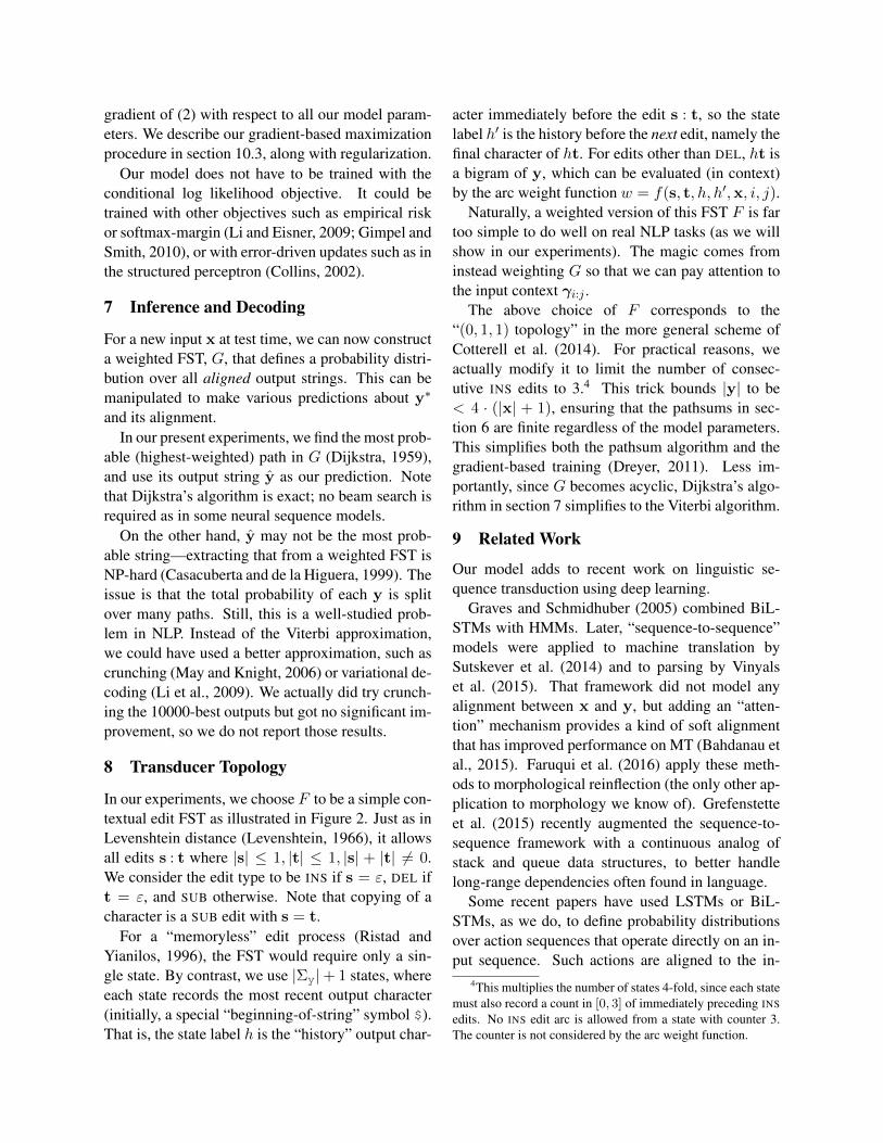
Our approach begins by hand-specifying an un-weighted finite-state transducer (FST), F , that non-deterministically maps any well-formed input x toall appropriate outputs y. An FST is a directed graphwhose vertices are called states, and whose arcs areeach labeled with some pair s :t, representing a pos-sible edit of a source substring s ∈ Σ∗x into a targetsubstring t ∈ Σ∗y. A path π from the FST’s initialstate to its final state represents an alignment of xto y, where x and y (respectively) are the concate-nations of the s and t labels of the arcs along π. In

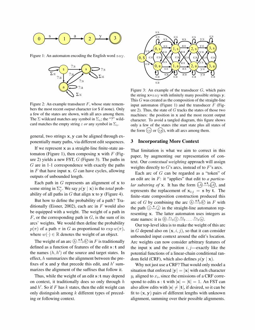
3210 s a y

Figure 1: An automaton encoding the English word say.

$

?:a

?:ss

a

?:s

Σ:ε

?:a

Σ:ε

?:s

?:aΣ:ε

Figure 2: An example transducer F , whose state remem-bers the most recent output character (or $ if none). Onlya few of the states are shown, with all arcs among them.The Σ wildcard matches any symbol in Σx; the “?” wild-card matches the empty string ε or any symbol in Σx.

general, two strings x,y can be aligned through ex-ponentially many paths, via different edit sequences.

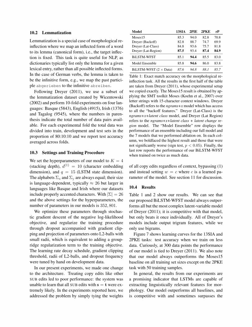
If we represent x as a straight-line finite-state au-tomaton (Figure 1), then composing x with F (Fig-ure 2) yields a new FST, G (Figure 3). The paths inG are in 1-1 correspondence with exactly the pathsin F that have input x. G can have cycles, allowingoutputs of unbounded length.

Each path in G represents an alignment of x tosome string in Σ∗y. We say p(y | x) is the total prob-ability of all paths in G that align x to y (Figure 4).

But how to define the probability of a path? Tra-ditionally (Eisner, 2002), each arc in F would alsobe equipped with a weight. The weight of a path inF , or the corresponding path in G, is the sum of itsarcs’ weights. We would then define the probabilityp(π) of a path π in G as proportional to expw(π),where w(·) ∈ R denotes the weight of an object.

The weight of an arc h© s:t−→ h′© in F is traditionallydefined as a function of features of the edit s : t andthe names (h, h′) of the source and target states. Ineffect, h summarizes the alignment between the pre-fixes of x and y that precede this edit, and h′ sum-marizes the alignment of the suffixes that follow it.

Thus, while the weight of an edit s :t may dependon context, it traditionally does so only through hand h′. So if F has k states, then the edit weight canonly distinguish among k different types of preced-ing or following context.

0, s

0, a

1, s

1, a

2, s

2, a 3, a

3, s

ε:sε:sε:sε:ss:s a:s y:s

s:ε a:ε y:ε

s:ε a:ε y:ε

ε:s

ε:aε:aε:aε:a s:a a:a y:a

ε:a ε:s ε:a ε:s ε:a ε:s ε:as:a

s:s

a:a

a:s

y:a

y:s0, $

ε:s

ε:a

s:a

s:s

Figure 3: An example of the transducer G, which pairsthe string x=say with infinitely many possible strings y.ThisGwas created as the composition of the straight-lineinput automaton (Figure 1) and the transducer F (Fig-ure 2). Thus, the state of G tracks the states of those twomachines: the position in x and the most recent outputcharacter. To avoid a tangled diagram, this figure showsonly a few of the states (the start state plus all states ofthe form i,s© or i,a©), with all arcs among them.

3 Incorporating More Context

That limitation is what we aim to correct in thispaper, by augmenting our representation of con-text. Our contextual weighting approach will assignweights directly to G’s arcs, instead of to F ’s arcs.

Each arc of G can be regarded as a “token” ofan edit arc in F : it “applies” that edit to a particu-lar substring of x. It has the form i,h© s:t−→j,h′©, andrepresents the replacement of xi:j = s by t. Thefinite-state composition construction produced thisarc of G by combining the arc h© s:t−→ h′© in F withthe path i© s

j© in the straight-line automaton rep-resenting x. The latter automaton uses integers asstate names: it is 0© x1−→ 1© x2−→ . . . xn−→ n©.

Our top-level idea is to make the weight of this arcin G depend also on (x, i, j), so that it can considerunbounded input context around the edit’s location.Arc weights can now consider arbitrary features ofthe input x and the position i, j—exactly like thepotential functions of a linear-chain conditional ran-dom field (CRF), which also defines p(y | x).

Why not just use a CRF? That would only model asituation that enforced |y| = |x| with each characteryi aligned to xi, since the emissions of a CRF corre-spond to edits s : t with |s| = |t| = 1. An FST canalso allow edits with |s| 6= |t|, if desired, so it can befit to (x,y) pairs of different lengths with unknownalignment, summing over their possible alignments.

0,$,0

0,s,1

1,$,0

1,s,1

2,$,0

2,s,1

0,a,2 1,a,2 2,a,2

0,i,3 1,i,3 2,i,3

0,d,4 1,d,4 2,d,4 3,d,4

3,$,0

3,s,1

3,a,2

3,i,3

ε:aε:s

ε:iε:d

ε:aε:s

ε:iε:d

ε:s

ε:s

ε:a ε:a

ε:i

ε:i

ε:d

ε:d

s:ε a:ε y:ε

s:ε a:ε y:ε

s:ε a:ε y:ε

s:ε a:ε y:ε

s:ε a:ε y:ε

s:s

a:a

y:ia:i

a:d

a:s

y:a

y:s

y:d

s:a

s:i

s:d

Figure 4: A compact lattice of the exponentially manypaths in the transducer G of Figure 3 that align in-put string x=say with output string y=said. To findp(y | x), we must sum over these paths (i.e., alignments).The lattice is created by composing G with y, which se-lects all paths in G that output y. Note that horizontalmovement makes progress through x; vertical movementmakes progress through y. The lattice’s states specializestates in G so that they also record a position in y.

A standard weighted FST F is similar to a dy-namic linear-chain CRF. Both are unrolled againstthe input x to get a dynamic programming lattice G.But they are not equivalent. By weighting G insteadof F , we combine the FST’s advantage (aligningunequal-length strings x,y via a latent path) withthe CRF’s advantage (arbitrary dependence on x).

To accomplish this weighting in practice, sec-tions 4–5 present a trainable neural architecture foran arc weight function w = f(s, t, h, h′,x, i, j).The goal is to extract continuous features from allof x. While our specific architecture is new, we arenot the first to replace hand-crafted log-linear mod-els with trainable neural networks (see section 9).

Note that as in a CRF, our arc weights cannotconsider arbitrary features of y, only of x. Still, aweight’s dependence on states h, h′ does let it de-pend on a finite amount of information about y (alsopossible in CRFs/HCRFs) and its alignment to x.

In short, our model p(y | x) makes the weight ofan s :t edit, applied to substring xi:j , depend jointlyon s :t and two summaries of the edit’s context:• a finite-state summary (h, h′) of its context in

the aligned (x,y) pair, as found by the FST F• a vector-valued summary of the context in x

only, as found by a recurrent neural network

The neural vector is generally a richer summary ofthe context, but it considers only the input-side con-text. We are able to efficiently extract these rich fea-tures from the single input x, but not from each ofthe very many possible outputs y. The job of theFST F is to compute additional features that alsodepend on the output.1 Thus our model of p(y | x)is defined by an FST together with a neural network.

4 Neural Context Features

Our arc weight function f will make use of a vec-tor γi:j (computed from x, i, j) to characterize thesubstring xi:j that is being replaced, in context. Wedefine γi:j as the concatenation of a left vector αj

(describing the prefix x0:j) and a right vector βi

(describing the suffix xi:n), which characterize xi:j

jointly with its left or right context. We use γj toabbreviate γj−1:j , just as xj abbreviates xj−1:j .

To extract αj , we read the string x one characterat a time with an LSTM (Hochreiter and Schmidhu-ber, 1997), a type of trainable recurrent neural net-work that is good at extracting relevant features fromstrings. αj is the LSTM’s output after j steps (whichread x0:j). Appendix A reviews how αj ∈ Rq iscomputed for j = 1, . . . , n using the recursive, dif-ferentiable update rules of the LSTM architecture.

We also read the string x in reverse with a secondLSTM. βi ∈ Rq is the second LSTM’s output aftern− i steps (which read reverse(xi:n)).

We regard the two LSTMs together as a BiLSTMfunction (Graves and Schmidhuber, 2005) that readsx (Figure 5). For each bounded-length substringxi:j , the BiLSTM produces a characterization γi:j

of that substring in context, in O(n) total time.We now define a “deep BiLSTM,” which stacks

up K BiLSTMs. This deepening is aimed at ex-tracting the kind of rich features that Sutskever et al.(2014) and Vinyals et al. (2015) found so effectivein a different structured prediction architecture.

The kth-level BiLSTM (Figure 6) reads a se-quence of input vectors x

(k)1 ,x

(k)2 , . . . ,x

(k)n ∈

Rd(k) , and produces a sequence of vectorsγ(k)1 ,γ

(k)2 , . . . ,γ

(k)n ∈ R2q. At the initial level

1Each arc of G is used in a known input context, but couldbe reused in many output contexts—different paths in G. Thosecontexts are only guaranteed to share h, h′. So the arc weightcannot depend on any other features of the output context.

s a y�1 �2

↵3↵2↵1

�3

↵0

�0

�1 �2 �3

Figure 5: A level-1 BiLSTM reading the word x=say.

↵(k)0 ↵

(k)1 ↵

(k)2 ↵

(k)3

�(k)3�

(k)2�

(k)1�

(k)0

�(k)1 �

(k)2

�(k�1)3�

(k�1)2�

(k�1)1

�(k)3

Figure 6: Level k > 1 of a deep BiLSTM. (We augmentthe shown input vectors with level k− 1’s input vectors.)

k = 1, we define x(1)j = exj ∈ Rd(1) , a vector

embedding of the character xj ∈ Σx. For k > 1, wetake x(k)

j to be γ(k−1)j , concatenated with x

(k−1)j for

good measure. Thus, d(k) = 2q + d(k−1).After this deep generalization, we define γi:j to be

the concatenation of all γ(k)i:j (rather than just γ(K)

i:j ).This novel deep BiLSTM architecture has more

connections than a pair of deep LSTMs, since α(k)j

depends not only on α(k−1)j but also on β

(k−1)j .

Thus, while we may informally regard α(k)j as be-

ing a deep summary of the prefix x0:j , it actuallydepends indirectly on all of x (except when k = 1).

5 The Arc Weight Function

Given the vector γi:j , we can now compute theweight of the edit arc i,h© s:t−→j,h′© in G, namely w =f(s, t, h, h′,x, i, j). Many reasonable functions arepossible. Here we use one that is inspired by the log-bilinear language model (Mnih and Hinton, 2007):

w = (es,γi,j , exi , exj+1) · rt,h,h′,type(s:t) (1)

The first argument to the inner product is an em-bedding es ∈ Rd(1) of the source substring s, con-catenated to the edit’s neural context and also (forgood measure) its local context.2 For example, if|s| = 1, i.e. s is a single character, then we would

2Our present implementation handles INS edits (for whichj = i) a bit differently, using (exi+1 ,γi:i+1, exi , exi+2) ratherthan (eε,γi:i, exi , exi+1). This is conveniently the same vectorthat is used for all other competing edits at this i position (as

use the embedding of that character as es. Notethat the embeddings es for |s| = 1 are also usedto encode the local context characters and the level-1 BiLSTM input. We learn these embeddings, andthey form part of our model’s parameter vector θ.

The second argument is a joint embedding of theother properties of the edit: the target substring t,the edit arc’s state labels from F , and the type of theedit (INS, DEL, or SUB: see section 8). When re-placing s in a particular context, which fixes the firstargument, we will prefer those replacements whoser embeddings yield a high inner product w. We willlearn the r embeddings as well; note that their di-mensionality must match that of the first argument.

The model’s parameter vector θ includes theO((d(K))2) parameters from the 2K LSTMs, whered(K) = O(d(1) + Kq). It also O(d(1)S) parame-ters for the embeddings es of the S different inputsubstrings mentioned by F , and O(d(K)T ) for theembeddings rt,h,h′,type(s:t) of the T “actions” in F .

6 Training

We train our model by maximizing the conditionallog-likelihood objective,∑

(x,y∗)∈dataset

log p(y∗ | x) (2)

Recall that p(y∗ | x) sums over all alignments. Asexplained by Eisner (2002), it can be computed asthe pathsum of the composition G ◦ y∗ (Figure 4),divided by the pathsum of G (which gives the nor-malizing constant for the distribution p(y | x)). Thepathsum of a weighted FST is the total weight of allpaths from the initial state to a final state, and can becomputed by the forward algorithm.3

Eisner (2002) and Li and Eisner (2009) also ex-plain how to compute the partial derivatives ofp(y∗ | x) with respect to the arc weights, essen-tially by using the forward-backward algorithm. Webackpropagate further from these partials to find the

they all have |s| = 1 in our present implementation); it providesan extra character of lookahead.

3If an FST has cycles, such as the self-loops in the exampleof Figure 3, then the forward algorithm’s recurrence equationsbecome cyclic, and must be solved as a linear system rather thansequentially. This is true regardless of how the FST’s weightsare defined. (For convenience, our experiments in this paperavoid cycles by limiting consecutive insertions: see section 8.)

gradient of (2) with respect to all our model param-eters. We describe our gradient-based maximizationprocedure in section 10.3, along with regularization.

Our model does not have to be trained with theconditional log likelihood objective. It could betrained with other objectives such as empirical riskor softmax-margin (Li and Eisner, 2009; Gimpel andSmith, 2010), or with error-driven updates such as inthe structured perceptron (Collins, 2002).

7 Inference and Decoding

For a new input x at test time, we can now constructa weighted FST, G, that defines a probability distri-bution over all aligned output strings. This can bemanipulated to make various predictions about y∗

and its alignment.In our present experiments, we find the most prob-

able (highest-weighted) path in G (Dijkstra, 1959),and use its output string y as our prediction. Notethat Dijkstra’s algorithm is exact; no beam search isrequired as in some neural sequence models.

On the other hand, y may not be the most prob-able string—extracting that from a weighted FST isNP-hard (Casacuberta and de la Higuera, 1999). Theissue is that the total probability of each y is splitover many paths. Still, this is a well-studied prob-lem in NLP. Instead of the Viterbi approximation,we could have used a better approximation, such ascrunching (May and Knight, 2006) or variational de-coding (Li et al., 2009). We actually did try crunch-ing the 10000-best outputs but got no significant im-provement, so we do not report those results.

8 Transducer Topology

In our experiments, we choose F to be a simple con-textual edit FST as illustrated in Figure 2. Just as inLevenshtein distance (Levenshtein, 1966), it allowsall edits s : t where |s| ≤ 1, |t| ≤ 1, |s| + |t| 6= 0.We consider the edit type to be INS if s = ε, DEL ift = ε, and SUB otherwise. Note that copying of acharacter is a SUB edit with s = t.

For a “memoryless” edit process (Ristad andYianilos, 1996), the FST would require only a sin-gle state. By contrast, we use |Σy|+ 1 states, whereeach state records the most recent output character(initially, a special “beginning-of-string” symbol $).That is, the state label h is the “history” output char-

acter immediately before the edit s : t, so the statelabel h′ is the history before the next edit, namely thefinal character of ht. For edits other than DEL, ht isa bigram of y, which can be evaluated (in context)by the arc weight function w = f(s, t, h, h′,x, i, j).

Naturally, a weighted version of this FST F is fartoo simple to do well on real NLP tasks (as we willshow in our experiments). The magic comes frominstead weighting G so that we can pay attention tothe input context γi:j .

The above choice of F corresponds to the“(0, 1, 1) topology” in the more general scheme ofCotterell et al. (2014). For practical reasons, weactually modify it to limit the number of consec-utive INS edits to 3.4 This trick bounds |y| to be< 4 · (|x| + 1), ensuring that the pathsums in sec-tion 6 are finite regardless of the model parameters.This simplifies both the pathsum algorithm and thegradient-based training (Dreyer, 2011). Less im-portantly, since G becomes acyclic, Dijkstra’s algo-rithm in section 7 simplifies to the Viterbi algorithm.

9 Related Work

Our model adds to recent work on linguistic se-quence transduction using deep learning.

Graves and Schmidhuber (2005) combined BiL-STMs with HMMs. Later, “sequence-to-sequence”models were applied to machine translation bySutskever et al. (2014) and to parsing by Vinyalset al. (2015). That framework did not model anyalignment between x and y, but adding an “atten-tion” mechanism provides a kind of soft alignmentthat has improved performance on MT (Bahdanau etal., 2015). Faruqui et al. (2016) apply these meth-ods to morphological reinflection (the only other ap-plication to morphology we know of). Grefenstetteet al. (2015) recently augmented the sequence-to-sequence framework with a continuous analog ofstack and queue data structures, to better handlelong-range dependencies often found in language.

Some recent papers have used LSTMs or BiL-STMs, as we do, to define probability distributionsover action sequences that operate directly on an in-put sequence. Such actions are aligned to the in-

4This multiplies the number of states 4-fold, since each statemust also record a count in [0, 3] of immediately preceding INS

edits. No INS edit arc is allowed from a state with counter 3.The counter is not considered by the arc weight function.

put. For example, Andor et al. (2016) score edit se-quences using a globally normalized model, whileYao and Zweig (2015) and Dyer et al. (2015) eval-uate the local probability of a transduction or pars-ing action given past actions (and any structure theybuilt) and future words. These architectures arepowerful because their LSTMs can globally assessthe output; but as a result they do not permit dynamicprogramming and must fall back on beam search.

Our use of dynamic programming for efficient ex-act inference has long been common in non-neuralarchitectures for sequence transduction, includingFST systems that allow “phrasal” replacements s : twhere |s|, |t| > 1 (Chen, 2003; Jiampojamarn etal., 2007; Bisani and Ney, 2008). Our work aug-ments these FSTs with neural networks, much asothers have augmented CRFs. In this vein, Durrettand Klein (2015) augment a CRF parser (Finkel etal., 2008) to score constituents with a feedforwardneural network. Likewise, FitzGerald et al. (2015)employ feedforward nets as a factor in a graphicalmodel for semantic role labeling. Many CRFs haveincorporated feedforward neural networks (Bridle,1990; Peng et al., 2009; Do and Artieres, 2010;Vinel et al., 2011; Fujii et al., 2012; Chen et al.,2015, and others). Some work augments CRFs withBiLSTMs: Huang et al. (2015) report results onpart-of-speech tagging and named entity recognitionwith a linear-chain CRF-BiLSTM, and Kong et al.(2015) on Chinese word segmentation and handwrit-ing recognition with a semi-CRF-BiLSTM.

10 Experiments

We evaluated our approach on two morphologi-cal generation tasks: reinflection (section 10.1) andlemmatization (section 10.2). In reinflection, thegoal is to transduce verbs from one inflected forminto another, whereas in lemmatization, the goal isto reduce an inflected verb to its root form.

We compare our WFST-LSTM against two stan-dard baselines, a WFST with hand-engineered fea-tures and the Moses phrase-based MT system(Koehn et al., 2007), as well as the more complexlatent-variable model of Dreyer et al. (2008). Thecomparison with Dreyer et al. (2008) is of noted in-terest since their latent variables are structured par-ticularly for morphological transduction tasks—we

are directly testing the ability of the LSTM to struc-ture its hidden layer as effectively as linguisticallymotivated latent-variables. Additionally, we providedetailed ablation studies and learning curves whichshow that our neural-WFSA hybrid model can gen-eralize even with very low amounts of training data.

10.1 Morphological Reinflection

Following Dreyer (2011), we conducted our ex-periments on the following transduction tasks fromthe CELEX (Baayen et al., 1993) morphologicaldatabase: 13SIA 7→ 13SKE, 2PIE 7→ 13PKE, 2PKE7→ z and rP 7→ pA.5 We refer to these tasks as 13SIA,2PIE, 2PKE and rP, respectively.

Concretely, each task requires us to map a Ger-man inflection into another inflection. Considerthe 13SIA task and the German verb abreiben

(“to rub off”). We require the model to learnto map a past tense form abrieb to a presenttense form abreibe—this involves a combinationof stem change and affix generation. Stickingwith the same verb abreiben, task 2PIE requiresthe model to transduce abreibt to abreiben—this requires an insertion and a substitution atthe end. The tasks 2PKE and rP are somewhatmore challenging since performing well on thesetasks requires the model to learn complex trans-duction: abreiben to abzureiben and abreibt

to abgerieben, respectively. These are complextransductions with phenomenon like infixation inspecific contexts (abzurieben) and circumfixation(abgerieben) along with additional stem and af-fix changes. See Dreyer (2011) for more details andexamples of these tasks.

We use the datasets of Dreyer (2011). Each exper-iment sampled a different dataset of 2500 examplesfrom CELEX, dividing this into 500 training + 1000validation + 1000 test examples. Like them, we re-port exact-match accuracy on the test examples, av-eraged over 5 distinct experiments of this form. Wealso report results when the training and validationdata are swapped in each experiment, which doublesthe training size.

5Glossary: 13SIA=1st/3rd sg. ind. past; 13SKE=1st/3rdsg. subjunct. pres.; 2PIE=2nd pl. ind. pres.; 13PKE=1st/3rdpl. subjunct. pres.; 2PKE=2nd pl. subjunct. pres.; z=infinitive;rP=imperative pl.; pA=past part.

10.2 Lemmatization

Lemmatization is a special case of morphological re-inflection where we map an inflected form of a wordto its lemma (canonical form), i.e., the target inflec-tion is fixed. This task is quite useful for NLP, asdictionaries typically list only the lemma for a givenlexical entry, rather than all possible inflected forms.In the case of German verbs, the lemma is taken tobe the infinitive form, e.g., we map the past partici-ple abgerieben to the infinitive abreiben.

Following Dreyer (2011), we use a subset ofthe lemmatization dataset created by Wicentowski(2002) and perform 10-fold experiments on four lan-guages: Basque (5843), English (4915), Irish (1376)and Tagalog (9545), where the numbers in paren-thesis indicate the total number of data pairs avail-able. For each experimental fold the total data wasdivided into train, development and test sets in theproportion of 80:10:10 and we report test accuracyaveraged across folds.

10.3 Settings and Training Procedure

We set the hyperparameters of our model to K = 4(stacking depth), d(1) = 10 (character embeddingdimension), and q = 15 (LSTM state dimension).The alphabets Σx and Σy are always equal; their sizeis language-dependent, typically ≈ 26 but larger inlanguages like Basque and Irish where our datasetsinclude properly accented characters. With |Σ| = 26and the above settings for the hyperparameters, thenumber of parameters in our models is 352, 801.

We optimize these parameters through stochas-tic gradient descent of the negative log-likelihoodobjective, and regularize the training procedurethrough dropout accompanied with gradient clip-ping and projection of parameters onto L2-balls withsmall radii, which is equivalent to adding a group-ridge regularization term to the training objective.The learning rate decay schedule, gradient clippingthreshold, radii of L2-balls, and dropout frequencywere tuned by hand on development data.

In our present experiments, we made one changeto the architecture. Treating copy edits like otherSUB edits led to poor performance: the system wasunable to learn that all SUB edits with s = t were ex-tremely likely. In the experiments reported here, weaddressed the problem by simply tying the weights

Model 13SIA 2PIE 2PKE rPMoses15 85.3 94.0 82.8 70.8Dreyer (Backoff) 82.8 88.7 74.7 69.9Dreyer (Lat-Class) 84.8 93.6 75.7 81.8Dreyer (Lat-Region) 87.5 93.4 87.4 84.9

BiLSTM-WFST 85.1 94.4 85.5 83.0

Model Ensemble 85.8 94.6 86.0 83.8

BiLSTM-WFST (2 × Data) 87.6 94.8 88.1 85.7

Table 1: Exact match accuracy on the morphological re-inflection task. All the results in the first half of the tableare taken from Dreyer (2011), whose experimental setupwe copied exactly. The Moses15 result is obtained by ap-plying the SMT toolkit Moses (Koehn et al., 2007) overletter strings with 15-character context windows. Dreyer(Backoff) refers to the ngrams+x model which has accessto all the “backoff features.” Dreyer (Lat-Class) is thengrams+x+latent class model, and Dreyer (Lat Region)refers to the ngrams+x+latent class + latent change re-gion model. The “Model Ensemble” row displays theperformance of an ensemble including our full model andthe 7 models that we performed ablation on. In each col-umn, we boldfaced the highest result and those that werenot significantly worse (sign test, p < 0.05). Finally, thelast row reports the performance of our BiLSTM-WFSTwhen trained on twice as much data.

of all copy edits regardless of context, bypassing (1)and instead setting w = c where c is a learned pa-rameter of the model. See section 11 for discussion.

10.4 Results

Table 1 and 2 show our results. We can see thatour proposed BiLSTM-WFST model always outper-forms all but the most complex latent-variable modelof Dreyer (2011); it is competitive with that model,but only beats it once individually. All of Dreyer’smodels include output trigram features, while weonly use bigrams.

Figure 7 shows learning curves for the 13SIA and2PKE tasks: test accuracy when we train on lessdata. Curiously, at 300 data points the performanceof our model is tied to Dreyer (2011). We also notethat our model always outperforms the Moses15baseline on all training set sizes except on the 2PKEtask with 50 training samples.

In general, the results from our experiments area promising indicator that LSTMs are capable ofextracting linguistically relevant features for mor-phology. Our model outperforms all baselines, andis competitive with and sometimes surpasses the

Model Basque English Irish Tagalog

Base (W) 85.3 91.0 43.3 0.3WFAffix (W) 80.1 93.1 70.8 81.7ngrams (D) 91.0 92.4 96.8 80.5

ngrams + x (D) 91.1 93.4 97.0 83.0ngrams + x + l (D) 93.6 96.9 97.9 88.6

BiLSTM-WFST 91.5 94.5 97.9 97.4Table 2: Lemmatization results on Basque, English, Irishand Tagalog. Comparison systems marked with (W) aretaken from Wicentowski (2002) and systems marked witha (D) are taken from Dreyer (2011). We outperform base-lines on all languages and are competitive with the latent-variable approach (ngrams + x + l), beating it in twocases: Irish and Tagalog.

50100 300 500 100055

60

65

70

75

80

85

90

Acc

ura

cy

2PKE

50100 300 500 100072

74

76

78

80

82

84

86

8813SIA

BiLSTM-WFST

Dreyer (Lat-Region)

Dreyer (Backoff)

Moses15

Figure 7: Learning Curves

latent-variable model of Dreyer et al. (2008) withoutany of the hand-engineered features or linguisticallyinspired latent variables.

On morphological reinflection, we outperform allof Dreyer et al’s models on 2PIE, but fall short ofhis latent-change region model on the other tasks(outperforming the other models). On lemmatiza-tion, we outperform all of Wicentowski’s models onall the languages, and all of Dreyer et al.’s modelson Irish and Tagalog, but not Dreyer et al.’s latent-variable approach on Basque or English. This sug-gests that perhaps further gains are possible throughusing something like Dreyer’s FST as our F . Indeed,this would be compatible with recent work that getsbest results by combining automatically learned neu-ral features and hand-engineered features.

10.5 Analysis of Results

We analyzed our lemmatization errors for all the lan-guages on one fold of the datasets. On the Englishlemmatization task, 7 of our 27 errors simply copiedthe input word to the output: ate, kept, went,

taught, torn, paid, strung. This suggests

Systems 13SIA 2PIE 2PKE rPDeep BiLSTM w/ Tying 86.8 94.8 87.9 81.1

Deep BiLSTM (No Context) 86.5 94.3 87.8 78.8Deep BiLSTMs w/o Copying 86.5 94.6 86.5 80.7Shallow BiLSTM 86.4 94.7 86.1 80.6Bi-Deep LSTM 86.1 94.2 86.5 78.6Deep MonoLSTM 84.0 93.8 85.6 67.3Shallow MonoLSTM 84.2 94.5 84.9 68.2No LSTM (Local Context) 83.6 88.5 83.2 68.0Deep BiLSTM w/o Tying 69.7 78.5 77.9 66.7No LSTM (No Context) 70.7 84.9 72.4 64.1

Seq2Seq-Att-4Layer 76.0 91.4 81.2 79.3Seq2Seq-Att-1Layer 77.2 89.6 82.1 79.1Seq2Seq-4Layer 2.5 5.2 11.5 6.4Seq2Seq-1Layer 9.1 11.1 14.1 11.9

Table 3: Ablation results for reinflection: Exact-matchaccuracy on the validation data of different systems. Likethe test accuracies, these average over 5 experiments.

that our current aggressive parameter tying for copyedits may predict a high probability for a copy editeven in contexts that should not favor it.

Also we found that the FST sometimes pro-duced non-words while lemmatizing the inputverbs. For example it mapped picnicked 7→picnick, happen 7→ hapen, exceed 7→ excy

and lining 7→ lin. Since these strings would berare in a corpus, many such errors could be avoidedby a reranking approach that combined the FST’spath score with a string frequency feature.

In order to better understand our architecture andthe importance of its various components, we per-formed an ablation study on the validation por-tions of the morphological induction datasets, shownin Table 3. We can see in particular that using a BiL-STM instead of an LSTM, increasing the depth ofthe network, and including local context all helpedto improve the final accuracy.

“Deep BiLSTM w/ Tying” refers to our completemodel. The other rows are ablation experiments—architectures that are the same as the first row exceptin the specified way. “Deep BiLSTM (No Context)”omits local context exi , exj+1 from (1). “Deep BiL-STMs w/o Copying” does not concatenate a copy ofx(k−1)i into x

(k)i and simplifies γi:j to be γ

(K)i:j only.

“Shallow BiLSTM” reduces K from 4 to 1. “Bi-Deep LSTM” replaces our deep BiLSTM with twodeep LSTMs that run in opposite directions but donot interact with each other. “Deep MonoLSTM”redefines βi to be the empty vector,g i.e. it replaces

the deep BiLSTM with a deep left-to-right LSTM.“Shallow MonoLSTM” replaces the deep BiLSTMwith a shallow left-to-right LSTM. “No LSTM (Lo-cal Context)” omits γi:j from the weight function al-together. “Deep BiLSTM w/o Tying” does not usethe parameter tying heuristic for copy edits. “NoLSTM (No Context)” is the simplest model that weconsider. It removes γi:j , exi and exj+1 and in fact,it is precisely a weighting of the edits in our origi-nal FST F , without further considering the contextin which an edit is applied.

Finally, to compare the performance of ourmethod to baseline neural encoder-decoder models,we trained 1-layer and 4-layer neural sequence-to-sequence models with and without attention, us-ing the publicly available morph-trans toolkit(Faruqui et al., 2016). We show the performanceof these models in the lower half of the table. Theresults consistently show that sequence-to-sequencetransduction models that lack the constraints ofmonotonic alignment perform worse than our pro-posed models on morphological transduction tasks.

11 Future Work: Possible Extensions

As neither our FST-LSTM model or the latent-variable WFST model of Dreyer et al. (2008) uni-formly outperforms the other, a future direction isto improve the FST we use in our model—e.g., byaugmenting its states with explicit latent variables.Other improvements to the WFST would be to in-crease the amount of history h stored in the states,and to allow s, t to be longer than a single character,which would allow the model to segment x.

We are not committed to the arc weight functionin (1), and we imagine that further investigation herecould improve performance. The goal is to definethe weight of the arc h© s:t−→ h′© in the context summa-rized by αi,βj (the context around xi:j = s) and/orby αj ,βi (which incorporate s as well).

Eq. (1) could be replaced by any parametric func-tion of the variables (s, t, h, h′,αi,αj ,βi,βj)—e.g., a neural network or a multilinear function. Thisfunction might depend on learned embeddings of theseparate objects s, t, h, h′, but also on learned jointembeddings of pairs of these objects (which addsfiner-grained parameters), or hand-specified proper-ties of the objects such as their phonological features

(which adds backoff parameters).Such a scheme might set w = f(c) ·g(r), where r

is some encoding of the arc (s, t, h, h′), c is someencoding of the context (αi,αj ,βi,βj , s, h, h

′),and f and g are learned linear or nonlinear vector-valued functions. Note that this formulation lets theobjects s, h, h′ play a dual role—they could appearas part of the arc and also as part of the context.This is because we must judge whether s = xi:j

(with “label” h©−→ h′©) is an appropriate input seg-ment given the string context around xi:j , but if thissegment is chosen, in turn it provides additional con-text to judge whether t is an appropriate output.

One could also revisit the stacking mechanism.Rather than augmenting a character xj at the nextlevel with its context (αj ,βi) (where i = j−1), onemight augment it with the richer context f(c) or eventhe arc-in-context representation f(c)�g(r), wheret, h, h′ are chosen to maximize w (max-pooling).

High-probability edits s : t typically have t ≈ s:a perfect copy, or a modified copy that changes justone or two features such as phonological voicing ororthographic capitalization. So we may wish to learna shared set of embeddings for Σx ∪ Σy, and makethe weight of s : t arcs depend on features of the“discrepancy vector” et − es, such as this vector’scomponents6 and their absolute magnitudes, whichwould signal discrepancies of various sorts.

12 Conclusions

We have presented a hybrid FST-LSTM architec-ture for string-to-string transduction tasks. Thisapproach combines classical finite-state approachesto transduction and newer neural approaches. Weweight the same FST arc differently in different con-texts, and use LSTMs to automatically extract fea-tures that determine these weights. This reduces theneed to engineer a complex topology for the FSTor to hand-engineer its weight features. We evalu-ated one such model on the tasks of morphologicalreinflection and lemmatization. Our approach out-performs several baselines and is competitive with(and sometimes surpasses) a latent-variable modelhand-crafted for morphological transduction tasks.7

6In various directions—perhaps just the basis directions,which might come to encode distinctive features, via training.

7We have released our code for this paper atgithub.com/se4u/neural wfst.

Acknowledgements

This research was supported by the Defense AdvancedResearch Projects Agency under the Deep Explorationand Filtering of Text (DEFT) Program, agreement num-ber FA8750-13-2-001; by the National Science Founda-tion under Grant No. 1423276; and by a DAAD fellow-ship to the second author. We would like to thank MarkusDreyer for providing the datasets and Manaal Faruqui forproviding implementations of the baseline sequence-to-sequence models. Finally we would like to thank Mo Yu,Nanyun Peng, Dingquan Wang and Elan Hourticolon-Retzler for helpful discussions and early prototypes forsome of the neural network architectures.

ReferencesDaniel Andor, Chris Alberti, David Weiss, Aliaksei

Severyn, Alessandro Presta, Kuzman Ganchev, SlavPetrov, and Michael Collins. 2016. Globally nor-malized transition-based neural networks. Availableat arXiv.org as arXiv:1603.06042, March.

R. Harald Baayen, Richard Piepenbrock, and Rijn van H.1993. The CELEX lexical data base on CD-ROM.

Dzmitry Bahdanau, Kyunghyun Cho, and Yoshua Ben-gio. 2015. Neural machine translation by jointlylearning to align and translate. In Proceedings ofICLR.

Maximilian Bisani and Hermann Ney. 2008. Joint-sequence models for grapheme-to-phoneme conver-sion. Speech Communication, 50(5):434–451.

John S. Bridle. 1990. Training stochastic model recog-nition algorithms as networks can lead to maximummutual information estimation of parameters. In Pro-ceedings of NIPS, pages 211–217.

Francisco Casacuberta and Colin de la Higuera. 1999.Optimal linguistic decoding is a difficult compu-tational problem. Pattern Recognition Letters,20(8):813–821.

Liang-Chieh Chen, Alexander Schwing, Alan Yuille, andRaquel Urtasun. 2015. Learning deep structured mod-els. In Proceedings of ICML, pages 1785–1794.

Stanley F. Chen. 2003. Conditional and joint models forgrapheme-to-phoneme conversion. In Proceedings ofEUROSPEECH.

Michael Collins. 2002. Discriminative training meth-ods for hidden Markov models: Theory and experi-ments with perceptron algorithms. In Proceedings ofthe Conference on Empirical Methods in Natural Lan-guage Processing, Philadelphia, July.

Ryan Cotterell, Nanyun Peng, and Jason Eisner. 2014.Stochastic contextual edit distance and probabilisticFSTs. In Proceedings of ACL, pages 625–630, June.

E. W. Dijkstra. 1959. A note on two problems in con-nexion with graphs. Numerische Mathematik, 1(1).

Trinh-Minh-Tri Do and Thierry Artieres. 2010. Neu-ral conditional random fields. In Proceedings of AIS-TATS. JMLR.

Markus Dreyer, Jason R. Smith, and Jason Eisner. 2008.Latent-variable modeling of string transductions withfinite-state methods. In Proceedings of EMNLP, pages1080–1089, October.

Markus Dreyer. 2011. A Non-Parametric Model for theDiscovery of Inflectional Paradigms from Plain TextUsing Graphical Models over Strings. Ph.D. thesis,Johns Hopkins University, Baltimore, MD, April.

Greg Durrett and Dan Klein. 2015. Neural CRF parsing.In Proceedings of ACL.

Chris Dyer, Miguel Ballesteros, Wang Ling, AustinMatthews, and Noah A. Smith. 2015. Transition-based dependency parsing with stack long short-termmemory. In Proceedings of ACL-IJCNLP, pages 334–343, July.

Jason Eisner. 2002. Parameter estimation for probabilis-tic finite-state transducers. In Proceedings of ACL,pages 1–8, July.

Manaal Faruqui, Yulia Tsvetkov, Graham Neubig, andChris Dyer. 2016. Morphological inflection genera-tion using character sequence to sequence learning. InProceedings of NAACL. Code available at https://github.com/mfaruqui/morph-trans.

Jenny Rose Finkel, Alex Kleeman, and Christopher D.Manning. 2008. Efficient, feature-based, conditionalrandom field parsing. In Proceedings of ACL, pages959–967.

Nicholas FitzGerald, Oscar Tackstrom, KuzmanGanchev, and Dipanjan Das. 2015. Semantic rolelabeling with neural network factors. In Proceedingsof EMNLP, pages 960–970.

Yasuhisa Fujii, Kazumasa Yamamoto, and Seiichi Naka-gawa. 2012. Deep-hidden conditional neural fields forcontinuous phoneme speech recognition. In Proceed-ings of IWSML.

Kevin Gimpel and Noah A. Smith. 2010. Softmax-margin CRFs: Training log-linear models with costfunctions. In Proceedings of NAACL-HLT, pages 733–736, June.

Alex Graves and Jurgen Schmidhuber. 2005. Frame-wise phoneme classification with bidirectional lstmand other neural network architectures. Neural Net-works, 18(5):602–610.

Alex Graves. 2012. Supervised Sequence Labelling withRecurrent Neural Networks. Springer.

Edward Grefenstette, Karl Moritz Hermann, Mustafa Su-leyman, and Phil Blunsom. 2015. Learning to trans-duce with unbounded memory. In Proceedings ofNIPS, pages 1819–1827.

Sepp Hochreiter and Jurgen Schmidhuber. 1997. Longshort-term memory. Neural Computation.

Zhiheng Huang, Wei Xu, and Kai Yu. 2015. Bidi-rectional LSTM-CRF models for sequence tagging.arXiv preprint arXiv:1508.01991.

Sittichai Jiampojamarn, Grzegorz Kondrak, and TarekSherif. 2007. Applying many-to-many alignmentsand hidden Markov models to letter-to-phoneme con-version. In Proceedings of NAACL-HLT, pages 372–379.

Philipp Koehn, Hieu Hoang, Alexandra Birch, ChrisCallison-Burch, Marcello Federico, Nicola Bertoldi,Brooke Cowan, Wade Shen, Christine Moran, RichardZens, et al. 2007. Moses: Open source toolkitfor statistical machine translation. In Proceedings ofACL (Interactive Poster and Demonstration Sessions),pages 177–180.

Lingpeng Kong, Chris Dyer, and Noah A. Smith. 2015.Segmental recurrent neural networks. arXiv preprintarXiv:1511.06018.

Vladimir I. Levenshtein. 1966. Binary codes capable ofcorrecting deletions, insertions, and reversals. SovietPhysics Doklady, 10(8):707–710.

Zhifei Li and Jason Eisner. 2009. First- and second-orderexpectation semirings with applications to minimum-risk training on translation forests. In Proceedings ofEMNLP, pages 40–51, August.

Zhifei Li, Jason Eisner, and Sanjeev Khudanpur. 2009.Variational decoding for statistical machine transla-tion. In Proceedings of ACL, pages 593–601.

Jonathan May and Kevin Knight. 2006. A better n-bestlist: Practical determinization of weighted finite treeautomata. In Proceedings of NAACL, pages 351–358.

Andriy Mnih and Geoffrey Hinton. 2007. Three newgraphical models for statistical language modelling. InProceedings of ICML, pages 641–648. ACM.

Mehryar Mohri. 1997. Finite-state transducers in lan-guage and speech processing. Computational Linguis-tics, 23(2):269–311.

Jian Peng, Liefeng Bo, and Jinbo Xu. 2009. Conditionalneural fields. In Proceedings of NIPS, pages 1419–1427.

Eric Sven Ristad and Peter N. Yianilos. 1996. Learningstring edit distance. Technical Report CS-TR-532-96,Princeton University, Department of Computer Sci-ence, October. Revised October 1997.

Ilya Sutskever, Oriol Vinyals, and Quoc Le. 2014. Se-quence to sequence learning with neural networks. InProceedings of NIPS.

Antoine Vinel, Trinh Minh Tri Do, and Thierry Artieres.2011. Joint optimization of hidden conditional ran-dom fields and non-linear feature extraction. In Pro-ceedings of ICDAR, pages 513–517. IEEE.

Oriol Vinyals, Łukasz Kaiser, Terry Koo, Slav Petrov,Ilya Sutskever, and Geoffrey Hinton. 2015. Gram-mar as a foreign language. In Proceedings of NIPS,pages 2755–2763.

Richard Wicentowski. 2002. Modeling and LearningMultilingual Inflectional Morphology in a MinimallySupervised Framework. Ph.D. thesis, Johns HopkinsUniversity.

Kaisheng Yao and Geoffrey Zweig. 2015. Sequence-to-sequence neural net models for grapheme-to-phonemeconversion. In Proceedings of INTERSPEECH.

AppendicesA LSTM Formulas

Lowercase bold letters represent real vectors. Up-percase letters represent real matrices of the ap-prporiate dimension. Subscripts distinguish differ-ent vectors and matrices and not entries of a vec-tor. � denotes element-wise multiplication, and σis the sigmoid function σ(z) = 1

1+exp(−z) , appliedelement-wise. See Graves (2012) for the rationalebehind these definitions:

ci ← f i � ci−1 + ii � zi ∈ Rq (3)

αi ← oi � (2σ(2ci)− 1) ∈ Rq (4)

where xi ∈ Rd and

ii ← σ(Wixi + Uiαi−1 + di) ∈ Rq (5)

f i ← σ(Wfxi + Ufαi−1 + df) ∈ Rq (6)

zi ← 2σ(Wzxi + Uzαi−1 + dz)− 1 ∈ Rq (7)

oi ← σ(Woxi + Uoαi−1 + do) ∈ Rq (8)

ci denotes the LSTM’s hidden state, which is isobtained by interpolating ci−1 element-wise with avector zi that is derived from the input. We takec0 = 0. ci is then squashed and rescaled element-wise to determine the output αi. The vector zi de-pends on the entire previous output αi−1 and theentire input xi, as do the rescaling and interpo-lation coefficients—these non-element-wise defini-tions are in the last 4 lines. The parameter vec-tor θ includes the elements of Mm (for all M ∈{W,U,d} and m ∈ {i, f, o, z}) and the elements ofα0.