welfarecomparisonswithbounded...

Journal of Economic Theory 110 (2003) 309–336

Welfare comparisons with boundedequivalence scales

Marc Fleurbaey,a,b Cyrille Hagnere,b,c,� and Alain Trannoyb

aCATT, Universite de Pau, BP 1633, 64016 Pau Cedex, FrancebTHEMA, Universite de Cergy-Pontoise, 33, boulevard du Port, 95011 Cergy-Pontoise, Cedex, France

cOFCE, 69 quai d’Orsay, 75340 Paris Cedex 07, France

Received 12 February 1999; final version received 21 February 2002

Abstract

The paper considers the problem of comparing income distributions for heterogeneous

populations. The first contribution of this paper is a precise dominance criterion combined

with a simple algorithm for implementing the criterion. This criterion is shown to be

equivalent to unanimity among utilitarian social planners whose objectives are compatible

with given intervals of equivalence scales. The second contribution of the paper is to show that

this criterion is equivalent to dominance for two different families of social welfare functions,

one inspired by Atkinson and Bourguignon (in: G.R. Feiwel (Ed.), Arrow and Foundation of

the Theory of Economic Policy, Macmillan, London, 1987), in which household utility is a

general function of income and needs, and a second family inspired by Ebert (Soc. Choice

Welfare 16 (1999) 233), in which household utility is a function of equivalent incomes. Finally,

we extend our results to the case where the distributions of needs differ between the two

populations being compared.

r 2003 Elsevier Science (USA). All rights reserved.

JEL classification: D31; D63

Keywords: Heterogeneous population; Dominance; Equivalence scale; Welfare comparison

�Corresponding author.

E-mail addresses: [email protected] (M. Fleurbaey), [email protected]

(C. Hagner!e), [email protected] (A. Trannoy).

0022-0531/03/$ - see front matter r 2003 Elsevier Science (USA). All rights reserved.

doi:10.1016/S0022-0531(03)00035-8

1. Introduction

In the field of inequality and welfare comparisons, the focus of researchers isshifting away from the study of income distribution among identical agents to thestudy of populations of agents differing in non-income attributes like family size,age, sex, health, or more generally, needs. A growing number of papers deal with thisissue since the landmark article by Atkinson and Bourguignon [3]. A non exhaustivelist would include Bourguignon [6], Jenkins and Lambert [21], Shorrocks [27], Ebert[12–15], Moyes [23], Chambaz and Maurin [9], Ok and Lambert [24], and Cowell andMercader-Prats [10]. As the last authors wrote: ‘At the heart of any distributionalanalysis, there is the problem of allowing for differences in people’s non incomecharacteristics’ (p. 1).When needs differ across agents, there are basically two opposite ways to perform

inequality or welfare comparisons. The first one makes use of equivalence scales andhas been axiomatized by Ebert [13,14]. The second one investigates dominancecriteria by considering a wide class of household utility functions and the pioneersare without doubt Atkinson and Bourguignon [3], who refused to make welfarejudgments depend on equivalence scales, which they described as a floppy notion.The aim of this paper is to conciliate these two views by performing a dominanceanalysis over a range of equivalent scales. Let us present the advantages anddrawbacks of these two solutions before going into the details of our proposal.Equivalence scales are a means of converting ordinary incomes for households

with different needs into comparable quantities called equivalent incomes. Once anagreement about the choice of a specific equivalence scale has been reached one canperform a usual dominance analysis like Lorenz dominance [2] for an inequalitycomparison, or generalized Lorenz dominance [26] for a welfare comparison, basedon the vectors of equivalent incomes. The Lorenz curve is a helpful graphical deviceand retains its normative meaning, in terms of inequality and welfare, in this context:if the Lorenz curve (resp. generalized Lorenz curve) corresponding to an initialequivalent income distribution is above to the Lorenz curve (resp. generalizedLorenz curve) corresponding to a final one, then the inequality (resp. welfare) hasincreased (resp. decreased), and reciprocally. This approach, analysed by Ebert [14],is straightforward but the choice of a particular equivalence scale is alwayscontroversial. Many equivalence scales have been proposed (Buhmann et al. [8] list34) and it has been admitted that this multiplicity does not come from statisticalproblems but stems from a basic difficulty lying at the heart of the concept ofequivalence scales (see the discussion of Pollack and Wales [25] and Blundell andLewbell [5].Since there is not one ‘‘correct’’ equivalence scale, Atkinson and Bourguignon [3]

defend the idea that the use of such information has to be avoided in making welfarecomparisons. They explore less informationally demanding methods, which restupon general assumptions on derivatives of utility functions, and exhibit adominance condition, the sequential generalized Lorenz (SGL) criterion. The mainassumptions about utilities are that marginal utility increases with need, and that thesmaller the need is, the slower the marginal utility decreases. These assumptions

M. Fleurbaey et al. / Journal of Economic Theory 110 (2003) 309–336310

imply that social welfare is increased when a household makes a transfer of incomein favor of another household with less incomes and more needs, and that socialwelfare increases all the more as, when a household makes a transfer to a poorerhousehold with identical needs, these households have greater needs (see [15]).Bourguignon [6] has proposed a criterion that does not rely on the latter assumptionand therefore covers a broader class of utility functions.There is a cost to generality and the SGL criterion will fail to compare many

income distributions. The ranking generated is much more partial than the ordergenerated by the Lorenz curve for equivalent incomes. This is even more the case forBourguignon’s criterion, which is strictly more partial than the SGL criterion. Thisdrawback mainly comes from the fact that these criteria pay attention to utilityfunctions which may give any order of magnitude to the priority of households withgreater needs, even though many of these utility functions would be considered asunreasonable by all practitioners. Consider, for instance, utility functions such that asingle has the same marginal utility, or equivalently, the same social priority, as acouple with 10 times the same income. These utility functions are unreasonablebecause it would be easy to argue that the couple should not have a greater prioritywhen it has more than twice the single’s income. But they do belong to the class ofutility functions on which the SGL and the Bourguignon criteria rely.To admit that equivalence scales cannot be precisely measured is one thing,

another is to deny any empirical value to the equivalence scales widely used inapplied studies. For instance, all the equivalence scales exhibit returns to scale inhousehold size so that, for example, a family of two adults does not require twice theincome of a single person. The value 2 can be thus considered as a fairly large upperbound for computing the equivalent income of a couple (in terms of a single’sincome) while 21=4 can be seen as the lowest bound possible according to subjectiveequivalence scales (see [8] for details). As shown below, this kind of information canbe used in order to sharpen the class of admissible utility functions.Therefore, between the generalized Lorenz criterion applied to equivalent incomes

proposed by Ebert [14], and the sequential generalized Lorenz criterion of Atkinsonand Bourguignon [3], there is room for a middleway criterion whose properties areexplored in this paper. The need for an analysis of the sensitivity of the generalizedLorenz criterion, when applied to equivalent incomes, to the choice of theequivalence scale has already been emphasized by Kakwani [22] and Jenkins [19],who compare the results obtained with different equivalence scales. The morespecific idea of considering intervals of acceptable equivalence scales has beenpromoted by Cowell and Mercader-Prats [10] and Bradbury [7]. The firstcontribution of this paper is a precise dominance criterion combined with a simplealgorithm for implementing the criterion. This criterion is shown to be equivalent tounanimity among utilitarian social planners whose objectives are compatible withgiven intervals of equivalence scales. The second contribution of the paper is to showthat this criterion is equivalent to dominance for two different families of socialwelfare functions, one inspired by Atkinson and Bourguignon, in which householdutility is a general function of income and needs, and a second family inspired byEbert, in which household utility is a function of equivalent incomes. In this way,

M. Fleurbaey et al. / Journal of Economic Theory 110 (2003) 309–336 311

this paper builds a bridge between these two approaches, which have so far beenstudied separately.It should be stressed that the criterion uncovered in this paper does not imply any

choice among the various possible ways of constructing intervals of equivalencescales. Whether they are based on more or less arbitrary value judgments or onempirical data about subjective welfare does not affect the validity of the criterion,which only requires the intervals to be precisely defined. Similarly, the utilitarianshape of the social objective considered in this paper does not imply anycommitment to the utilitarian philosophy. The only restriction is additiveseparability of the social objective, and the utility functions referred to in the sequelcan be viewed as representing either the households’ actual utility functions, or theplanner’s valuation functions embodying ethical principles such as a degree ofinequality aversion.The paper begins with the presentation of the framework and the introduction and

discussion of the families of utility functions appearing in the social welfare function,as well as of our central concept of social dominance. This is followed in Section 3 bythe main equivalence theorem featuring the dominance criterion, and thepresentation of the related algorithm. Section 4 shows that the dominance criterionis also equivalent to generalized Lorenz dominance applied to equivalent incomes,with bounded equivalence scales. An extension to the case where the distributions ofneeds can differ between the distributions being compared is provided in Section 5with a reexamination of assumptions and tools developed up to now. In particular,in line with the spirit of the paper, we make use of a condition which bounds thedifference of utility levels across groups.

2. Framework and ethical assumptions

2.1. Basic definitions

In this section and the next one, we will deal with a framework introduced byBourguignon [6] and we retain most of the notations. The population is divided intoK types, or groups of needs, where needs are ranked on a scale such that k ¼ 1corresponds to the least needy group and k ¼ K denotes the most needy group (thereader may think of k as an index of needs, such as family size). The living standardof a household which belongs to group k and has income y is evaluated by the utilityfunction Vðy; kÞ; which is supposed to be finite at 0 and twice continuouslydifferentiable in y for all k; while y is assumed to belong to Rþ: In the sequel, Vyðy; kÞand Vyyðy; kÞ will, respectively, denote the first and second order partial derivatives

of V with respect to y: Social welfare is evaluated by a utilitarian function such thatthe social welfare associated with an income distribution f and a utility function V is

WV ¼XK

k¼1pk

Z sk

0

fkðyÞVðy; kÞ dy; ð1Þ


where pk is the subgroup k’s population share, and fkðyÞ the income density functionof group k; with a finite support ½0; sk�: Let f ¼ ðf1;y; fKÞ denote the incomedistribution.Consider two income distributions f and f �: If we suppose that the distribution of

needs is the same in the two populations, the difference in social welfare between f

and f � is given and denoted by

DWV ¼XK

k¼1pk

Z %sk

0

DfkðyÞVðy; kÞ dy; ð2Þ

with DfkðyÞ ¼ fkðyÞ � f �k ðyÞ and %sk ¼ maxðsk; s�kÞ; where s�k is the upper bound of the

support of f �k :

Dominance is defined as unanimity for a family of social welfare functions basedon different utility functions.

Definition 2.1. f dominates f � for a family V of utility functions if and only ifDWVX0 for all utility functions V in V: This is denoted f DV f �:

The family of utility functions on which we focus in this paper is introduced in thenext subsection.

2.2. Family of utility functions

In this subsection we deal with the general family of functions a la Atkinson–Bourguignon, and introduce assumptions on marginal utilities based on variousethical principles. These assumptions determine the subfamily of utility functionswith respect to which dominance will be studied in the next section.The first assumption simply means that more income is better, and can be viewed

as reflecting a kind of Pareto principle with respect to incomes, implying that givingmore income to any part of the population is socially better.

U1. Vyðy; kÞX0; 8yARþ; 8kAf1;y;Kg:

The second assumption states that marginal utility is decreasing, and can berelated to the Pigou–Dalton transfer principle, according to which it is a good thingto make transfers from rich to poor households of the same type.

U2. Vyyðy; kÞp0; 8yARþ; 8kAf1;y;Kg:

Our next assumptions have to do with comparisons of marginal utilities forhouseholds of different types. It may be easier to start with an example. Suppose thatthe experts’ opinions about the relative needs for couples, taking singles as thereference type of household, fall down into the interval ½1:3; 1:7�: This means that,with respect to a single with an income of $10,000, all experts agree that a couplewith income less than $13,000 is poorer, or should be given a higher priority (socialmarginal value), and they all agree that a couple with income above $17,000 is richer,


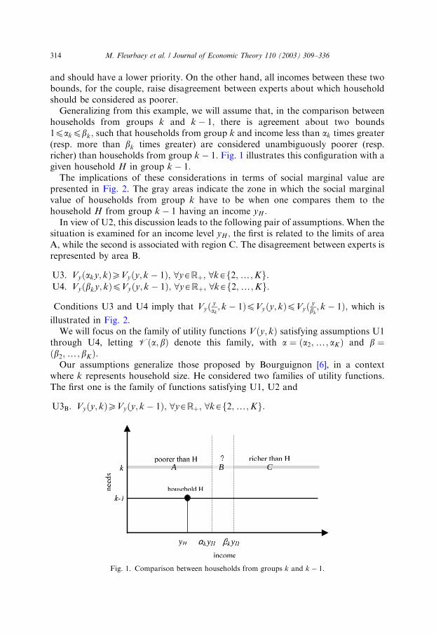
and should have a lower priority. On the other hand, all incomes between these twobounds, for the couple, raise disagreement between experts about which householdshould be considered as poorer.Generalizing from this example, we will assume that, in the comparison between

households from groups k and k � 1; there is agreement about two bounds1pakpbk; such that households from group k and income less than ak times greater(resp. more than bk times greater) are considered unambiguously poorer (resp.richer) than households from group k � 1: Fig. 1 illustrates this configuration with agiven household H in group k � 1:The implications of these considerations in terms of social marginal value are

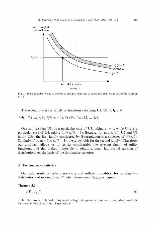
presented in Fig. 2. The gray areas indicate the zone in which the social marginalvalue of households from group k have to be when one compares them to thehousehold H from group k � 1 having an income yH :In view of U2, this discussion leads to the following pair of assumptions. When the

situation is examined for an income level yH ; the first is related to the limits of areaA, while the second is associated with region C. The disagreement between experts isrepresented by area B.

U3. Vyðaky; kÞXVyðy; k � 1Þ; 8yARþ; 8kAf2;y;Kg:U4. Vyðbky; kÞpVyðy; k � 1Þ; 8yARþ; 8kAf2;y;Kg:

Conditions U3 and U4 imply that Vyð yak; k � 1ÞpVyðy; kÞpVyð y

bk; k � 1Þ; which is

illustrated in Fig. 2.We will focus on the family of utility functions Vðy; kÞ satisfying assumptions U1

through U4, letting Vða; bÞ denote this family, with a ¼ ða2;y; aKÞ and b ¼ðb2;y; bKÞ:Our assumptions generalize those proposed by Bourguignon [6], in a context

where k represents household size. He considered two families of utility functions.The first one is the family of functions satisfying U1, U2 and

U3B: Vyðy; kÞXVyðy; k � 1Þ; 8yARþ; 8kAf2;y;Kg:

y α y β y

A B C

Fig. 1. Comparison between households from groups k and k � 1:


The second one is the family of functions satisfying U1, U2, U3B and

U4B: Vyðy; kÞpVyðk�1k

y; k � 1Þ; 8yARþ; 8kAf2;y;Kg:

One can see that U3B is a particular case of U3, taking ak ¼ 1; while U4B is aparticular case of U4, taking bk ¼ k=ðk � 1Þ: Because, for any akX1; U2 and U3imply U3B; the first family considered by Bourguignon is a superset of Vða; bÞ:Similarly, if 1pakpbkpk=ðk � 1Þ; the same holds for the second family.1 Therefore,our approach allows us to restrict considerably the relevant family of utilityfunctions, and this makes it possible to obtain a much less partial ranking ofdistributions on the basis of the dominance criterion.

3. The dominance criterion

Our main result provides a necessary and sufficient condition for ranking twodistributions of income f and f � when dominance DVða;bÞ is required.

Theorem 3.1.

f DVða;bÞf� ðAÞ

y α y β y

A

C

B

Fig. 2. Social marginal value of income in group k relatively to social marginal value of income in group

k � 1:

1 In other words, U3B and UB4B imply a larger disagreement between experts, which would be

illustrated in Figs. 1 and 2 by a larger area B.


is equivalent to

XK

k¼1pkDHkðxkÞp0 8ðxkÞk¼1;y;K ðBÞ

such that

akxk�1pxkpbkxk�1 8k ¼ 2;y;K ;

and

0px1pmax %s1;%s2

b2;

%s3

b2b3;y;

%sK

b2b3ybK

� �;

where DHkðxÞ ¼R x

0

R y

0DfkðzÞ dz dy:

Proof. Sufficiency: Condition (B) implies (A). Let us introduce for all k the followingfunctions, defined on Rþ:

V nðy; kÞ ¼ Vðy; kÞ þ lk

nlog

y

lk

þ 1

� �ð3Þ

with l1X1; aklk�1plkpbklk�1 for all k ¼ 2;y;K ; and n40:The first and second derivatives of Vnðy; kÞ are, respectively,

V ny ðy; kÞ ¼ Vyðy; kÞ þ 1

nð ylkþ 1Þ

and

V nyyðy; kÞ ¼ Vyyðy; kÞ � 1

nlkð ylkþ 1Þ2

:

One checks that, for all functions Vðy; kÞ belonging to the family Vða; bÞ; Vnðy; kÞsatisfy assumptions U3, U4, and the strict versions of U1 and U2, respectively,denoted U1� and U2�; for all n40:We will first prove that condition (B) is sufficient for dominance for any utility

functions V nðy; kÞ satisfying U1�; U2�; U3 and U4. Let us fix n:Rewriting expression (2) for functions V nðy; kÞ; we have

DWVn ¼XK

k¼1pk

Z %sk

0

DfkðyÞVnðy; kÞ dy: ð4Þ

Integrating by parts expression (4) and using the finiteness of Vnðy; kÞ at 0 and thefact that DFkð0Þ ¼ DFkð%skÞ ¼ 0 8k; we obtain

DWVn ¼ �XK

k¼1

Z %sk

0

Vny ðy; kÞpkDFkðyÞ dy: ð5Þ

Since Vny ðy; kÞ is continuous and strictly monotonous for all k; assumptions U3 and

U4 are satisfied if and only if there exists for all kAf2;y;Kg; a continuous function


jkðyÞ such that

akypjkðyÞpbky 8yARþ; ð6aÞ

and

V ny ðy; k � 1Þ ¼ V n

y ðjkðyÞ; kÞ 8yARþ: ð6bÞ

Notice that functions Vny ðy; kÞ can then be written, for all kAf1;y;K � 1g;

V ny ðy; kÞ ¼Vn

y ðjkþ1ðyÞ; k þ 1Þ ¼ V ny ðjkþ23jkþ1ðyÞ; k þ 2Þ ¼ ?

¼Vny ðjK3jK�13?3jkþ1ðyÞ;KÞ: ð7Þ

Moreover, jkðyÞ is differentiable because V ny ðy; kÞ is. So that expression (6b) implies

V nyyðy; k � 1Þ ¼ j0

kðyÞV nyyðjkðyÞ; kÞ: Thus, U2� requires j0

kðyÞ40; 8yARþ;

8kAf2;y;Kg:Since DFkðyÞ ¼ 0 8yX%sk; 8k; expression (5) can be written as

DWVn ¼ �XK

k¼1

Z bk

0

V ny ðy; kÞpkDFkðyÞ dy ð8Þ

with bkX%sk for all k:

Let us take b1 ¼ maxð%s1; %s2a2;%s3

a2a3;y; %sK

a2a3yaKÞ and bk ¼ jkðbk�1Þ; 8kAf2;y;Kg:

These expressions combined with condition (6a) guarantee that bkX%sk for all k:Let j1ðyÞ ¼ y and define ckðyÞ ¼ jk3jk�13?3j1ðyÞ for all k41 and c1ðyÞ ¼

j1ðyÞ: Thus, we can write bk ¼ ckðb1Þ for all k: Moreover, one can remark thatckð0Þ ¼ 0 for all k: Thus, introducing formula (7) in expression (8) leads to

DWVn ¼ �XK�1

k¼1

Z ckðb1Þ

ckð0ÞpkDFkðyÞVn

y ðjK3jK�13?3jkþ1ðyÞ;KÞ dy

�Z cK ðb1Þ

ckð0ÞpKDFKðyÞVn

y ðy;KÞ dy:

By a change of variable, and according to the fact that jK3jK�13?3jkþ1ðckðyÞÞ ¼cKðyÞ; it follows:

DWVn ¼ �XK

k¼1

Z b1

0

pkDFkðckðyÞÞV ny ðcKðyÞ;KÞc0

kðyÞ dy:


Integrating by parts leads to

DWVn ¼ �XK

k¼1pkDHkðckðb1ÞÞVn

y ðb1;KÞ

þXK

k¼1

Z b1

0

pkDHkðckðyÞÞc0KðyÞV n

yyðcKðyÞ;KÞ dy

¼ � V ny ðb1;KÞ

XK

k¼1pkDHkðckðb1ÞÞ

þZ b1

0

c0KðyÞVn

yyðcKðyÞ;KÞXK

k¼1pkDHkðckðyÞÞ dy:

Since jkðyÞ is strictly increasing for all k; c0KðyÞ40: Consequently, a sufficient

condition for f to dominate f � for all utility functions Vn satisfying U1�; U2�; U3and U4 is

XK

k¼1pkDHkðjk3jk�13?3j2ðyÞÞp0; ð9Þ

for all yA½0;maxð%s1; %s2a2;%s3

a2a3;y; %sK

a2a3yaKÞ�; and all functions jk such that

akypjkðyÞpbky; 8kAf2;y;Kg:By setting x1 ¼ y and xk ¼ jkðxk�1Þ for all kAf2;y;Kg; it follows that this

expression is equivalent to

XK

k¼1pkDHkðxkÞp0 8ðxkÞk¼1;y;K

such that

0px1pmax %s1;%s2

a2;

%s3

a2a3;y;

%sK

a2a3yaK

� �;

and

akxk�1pxkpbkxk�1 8k ¼ 2;y;K :

Moreover, since functions DHk are constant above %sk; it is not necessary to check the

conditions for some x1 larger than maxð%s1; %s2b2;%s3

b2b3;y; %sK

b2b3ybKÞ: Therefore, condition

(B) is sufficient.It remains to prove that (B) is also sufficient when we consider functions Vðy; kÞ in

Vða; bÞ: For this, we apply a corollary of the dominated convergence theorem (see[1, Theorem 10.29, p. 273]).According to expression (3), it is clear that limn-N V nðy; kÞ ¼ Vðy; kÞ 8y; 8k:

Since by assumption, Vðy; kÞ and functions lk

nlogð y

lkþ 1Þ are bounded for y

belonging to ½0; %sk�; so are Vnðy; kÞ: It is also the case for functions DfkðyÞ: Then, the


dominated convergence theorem implies that

limn-N

Z %sk

0

Vnðy; kÞDfkðyÞ dy ¼Z %sk

0

Vðy; kÞDfkðyÞ dy; for all k:

Consequently, limn-N DWVn ¼ DWV : Moreover, if condition (B) holds thenDWVnX0 for all n40 and therefore (B) is a sufficient condition for f to dominatef � for all utility functions V satisfying U1, U2, U3 and U4.

Necessity: (A) implies (B). Suppose f DVða;bÞf� and condition (B) is not verified.

Thus, there exists a K-vector ðe1; e2;y; eKÞ such that

e1A 0;max %s1;%s2

b2;

%s3

b2b3;y;

%sK

b2b3ybK

� �� ; ð10aÞ

akek�1pekpbkek�1 for all k ¼ 2;y;K ; ð10bÞ

and

XK

k¼1pkDHkðekÞ40: ð10cÞ

Consider the following function:

Vðy; kÞ ¼ ekUy

ek

� �ð11Þ

with akek�1pekpbkek�1 for all k ¼ 2;y;K ; e140; and UðxÞ a twice differentiablefunction such that U 0ðxÞX0; and U 00ðxÞp0 for all xX0: One checks that Vðy; kÞsatisfies assumptions U1 to U4.Now, consider a function U0ðxÞ such that

U 00ðxÞ ¼

1 if xp1� e;1e ð1� xÞ if xAð1� e; 1�;0 if x41;

8><>: ð12Þ

where eAð0; 1�:Recall that, since DfkðyÞ ¼ 0 8y4%sk; 8k; one can write

DWV0¼

XK

k¼1pk

Z %sk

0

DfkðyÞekU0y

ek

� �dy ¼

XK

k¼1pk

Z bk

0

DfkðyÞekU0y

ek

� �dy

with bkX%sk: In particular, we can choose bk such that ekpbk for all k: Thus,integrating twice by parts gives

DWV0¼ �

XK

k¼1

1

eek

Z ek

ekð1�eÞpkDHkðyÞ dy


which tends to �PK

k¼1 pkDHkðekÞ when e tends to 0. Therefore, there exists e suchthat

DWV0o� l

XK

k¼1pkDHkðekÞ ð13Þ

where 0olo1:U0 is not twice differentiable, but for any e and any l; one can find a twice

differentiable function U arbitrarily close to U0; so that

jDWV � DWV0j ¼

XK

k¼1pk

Z %sk

0

DfkðyÞek Uy

ek

� �� U0

y

ek

� �� dy

o lXK

k¼1pkDHkðekÞ: ð14Þ

Since DWV � DWV0pjDWV � DWV0

j; we deduce from (13) and (14) that one can

find functions Vðy; kÞ satisfying assumptions U1–U4 such that DWVoDWV0þ

lPK

k¼1 pkDHkðekÞo0; in contradiction with f DVða;bÞf�: &

Our condition generalizes the two conditions obtained by Bourguignon [6]:XK

k¼1pkDHkðxkÞp0; 8ðxkÞk¼1;y;K

such that xkXxk�1 ðk ¼ 2;y;KÞ and x1A½0; %s1�;

XK

k¼1pkDHkðxkÞp0 8ðxkÞk¼1;y;K such that xk�1pxkp

k

k � 1xk�1

ðk ¼ 2;y;KÞ and x1A 0;max %s1;1

2%s2;y;

K � 1

K%sK

� �� :

The first criterion corresponds, in our framework, to the case when ak ¼ 1 andbk-þN for all k ¼ 2;y;K : Regarding the second condition, it concerns the case

ak ¼ 1 and bk ¼ kk�1: A byproduct of the proof of Theorem (3.1) is to provide a more

direct proof of the Bourguignon’s theorem [6, p. 73].Atkinson-Bourguignon [3] criterion deals with the family of utility functions

satisfying assumptions U1, U2, U3B and the following additional condition:

UAB: Vyyðy; k � 1ÞXVyyðy; kÞ; 8yARþ; 8kAf2;y;Kg:

The criterion itself is that:XK

k¼1pkDHkðxkÞp0 8ðxkÞk¼1;y;K such that; for some l;

0 ¼ x1 ¼ ? ¼ xl�1pxl ¼ ? ¼ xK : ð15Þ


This criterion is not a particular case of ours, although it covers a very large family ofutility functions.Condition (B) is nothing else than the second degree stochastic dominance

condition restricted to income intervals. It can be given an intuitive interpretation byrecalling that (after integrating by part)XK

k¼1pkDHkðxkÞ ¼

XK

k¼1pk

Z xk

0

ðxk � yÞDfkðyÞ dy

and thatZ xk

0

ðxk � yÞfkðyÞ dy

is the absolute poverty gap for households of group k; taking xk as the poverty line.This link between second degree stochastic dominance and the absolute poverty gaphas been emphasized by Foster and Shorrocks [17]. Our condition thus states thatthe absolute poverty gap for the whole population must never be higher for f thanfor f �; for all poverty lines ðx1;y; xKÞ satisfying akxk�1pxkpbkxk�1 for all k ¼2;y;K : In contrast, Bourguignon’s first criterion refers to the poverty linessatisfying xk�1pxk for all k ¼ 2;y;K: And the Atkinson–Bourguignon approachdeals with poverty lines such that 0 ¼ x1 ¼ ? ¼ xk�1pxk ¼ ? ¼ xK for some k:Unfortunately, condition (B) is not implementable since it leads to checking an

infinity of conditions. One more step allows us to propose a more tractablecondition.For K ¼ 2; condition (B) is written as

p1DH1ðx1Þ þ p2DH2ðx2Þp0 8x1; x2

such that

a2x1px2pb2x1 and x1A 0;max %s1;%s2

b2

� �� : ð16Þ

It is straightforward to show that this condition is equivalent to the following:

p1DH1ðx1Þ þ maxx2A½a2x1;b2x1�

fp2DH2ðx2Þgp0 8x1A 0;max %s1;%s2

b2

� �� : ð17Þ

This implementable condition can be generalized in the following way.

Theorem 3.2. Define the following functions:

ZKðxÞ ¼ maxzA½aK x;bK x�

fpKDHKðzÞg;

ZkðxÞ ¼ maxzA½akx;bkx�

fpkDHkðzÞ þ Zkþ1ðzÞg 8k ¼ 2;y;K � 1:

Then a necessary and sufficient condition for f DVða;bÞf� is

p1DH1ðxÞ þ Z2ðxÞp0 8xA 0;max %s1;%s2

b2;

%s3

b2b3;y;

%sK

b2b3ybK

� �� : ðCÞ


Proof. Condition (C) can be written as

p1DH1ðxÞ þ maxx2A½a2x;b2x�


fp3DH3ðx3Þ þ?g� �

p0

8xA 0;max %s1;%s2

b2;

%s3

b2b3;y;

%sK

b2b3ybK

� �� : ð18Þ

This condition is clearly a particular case of condition (B), then by Theorem 3.1, thenecessity part is proved.For the converse, suppose that condition (B) is not verified, thus there exist a K-

vector ð %x1; %x2;y; %xKÞ such thatPK

k¼1 pkDHkð %xkÞ40 with ak %xk�1p %xkpbk %xk�1 8k ¼2;y;K and %x1A½0;maxð%s1; %s2b2;

%s3b2b3

;y; %sK

b2b3ybKÞ�:

Now, write condition (18) for x ¼ %x1:

p1DH1ð %x1Þ þ maxx2A½a2 %x1;b2 %x1�



p0:ð19Þ

Since %xkA½ak %xk�1; bk %xk�1� 8k ¼ 2;y;K ; and because of the max conditions, wehave

p1DH1ð %x1Þ þ maxx2A½a2 %x1;b2 %x1�



Xp1DH1ð %x1Þ þ p2DH2ð %x2Þ þ maxx3A½a3 %x2;b3 %x2�

fp3DH3ðx3Þ þ?g

Xp1DH1ð %x1Þ þ p2DH2ð %x2Þ þ p3DH3ð %x3Þ þ maxx4A½a4 %x3;b4 %x3�

fp4DH4ðx4Þ þ?g

^

X

XK

k¼1pkDHkð %xkÞ:

Thus, p1DH1ð %x1Þ þ Z2ð %x1Þ40: Consequently (C) implies (B) and by Theorem 3.1,(C) implies f DVða;bÞf

�: &

Theorem 3.2 thus yields a simple algorithm for the implementation of socialdominance DVða;bÞ:

4. Dominance with bounded equivalence scales

We now turn our attention to a second framework, proposed by Ebert [14]. It isbased on equivalence scales and is a particular case of the first framework.An equivalence scale is a list of numbers ek for k ¼ 1;y;K ; such that e1p?peK ;

and these numbers are interpreted in the following way. A household from group k

and with income y will be said to have an equivalent income equal to y=ek; andequivalent incomes are assumed to be directly comparable across types ofhouseholds. It is usual, in applied studies, to choose a reference group k0; which


amounts to letting ek0 ¼ 1: For instance, taking the group of singles as the reference,one can then view ek as the number of ‘‘equivalent adults’’ in households of group k;and y=ek is then the equivalent adult’s average income in the household.When a particular equivalence scale e ¼ ðe1;y; eKÞ is chosen, social welfare can

be computed by aggregating the utility levels of equivalent incomes over thepopulation, and Ebert [14] proposed to adopt the following household utilityfunction:

Vðy; kÞ ¼ ekUy

ek

� �;

where U is a twice differentiable real-valued function, which leads to the followingformula for the social welfare:2

WU ;e ¼XK

k¼1pk

Z %sk

0

fkðyÞekUy

ek

� �dy:

Now, a particular case of our approach in the previous sections is when ak ¼ bk

for all k ¼ 2;y;K : In this case, choose e1 arbitrarily, and for k ¼ 2;y;K ; computeek ¼ akek�1: One then obtains an equivalence scale e ¼ ðe1;y; eKÞ; and assumptionsU3 and U4 imply that for all yX0;

Vyðy; kÞ ¼ Vy

ek�1ek

y; k � 1

� �¼ ? ¼ Vy

e1

ek

y; 1

� �: ð20Þ

Define

UðyÞ ¼ 1

e1Vðe1y; 1Þ:

By integrating (20), up to a constant one gets Ebert’s formula

Vðy; kÞ ¼ ekUy

ek

� �:

In other words, this second approach based on a precise equivalence scale is just aparticular case of our approach in the first framework, and is obtained when theintervals ½ak; bk� boil down to points. In this section we study the relationshipbetween this approach in terms of equivalence scales, and the approach studied inthe first two sections, with non degenerate intervals.The comparison of two distributions f and f �; when a particular equivalence scale

is chosen, amounts to calculating the following difference:

DWU ;e ¼XK

k¼1pk

Z %sk

0

DfkðyÞekUy

ek

� �dy; ð21Þ

2Several forms of social welfare function have been discussed in the literature. Here, each household is

weighted by its equivalence scale. Other authors, like Glewwe [18], make use of a social welfare function in

which the weight is the number of persons in the household. But, as shown in [13], weighting by

equivalence scales is necessary and sufficient for a social welfare function to satisfy the condition that a

household with greater equivalent income has a lower social priority (social marginal value of income).


where DfkðyÞ is defined as previously. This expression has been written supposingthat the equivalence scale is known, but we can generalize it to the case when there issome uncertainty on the values of equivalence scales.3 Let Y be a set of equivalence

scales e ¼ ðe1;y; eKÞ; that is, a subset of vectors e from RKþþ; such that e1p?peK :

Now, consider the following new definition of social welfare dominance. Let Udenote a family of real-valued functions defined on Rþ:

Definition 4.1. f dominates f � for a family U of utility functions and a set Y ofequivalence scales if and only if DWU ;eX0 for all utility functions U in U and all K-

vectors e in Y: This is denoted f DU;Y f �:

As noticed above, one has DWU ;e ¼ DWV when Vðy; kÞ ¼ ekUð yekÞ: Consequently,

the dominance DU;Y is related to dominance DV: It turns out that, for some

appropriate families of functions, these two dominance conditions are equivalent. Inorder to obtain a precise statement of this fact, consider the class U2 of increasingand concave utility functions, namely the family of functions satisfying the followingassumptions:

fU1U1: U 0ðyÞX0 8yX0:fU2U2: U 00ðyÞp0 8yX0:

We propose to consider a particular setY defined in the following parametric way:

Yða; bÞ ¼ fðe1;y; eKÞ j akek�1pekpbkek�1 8k ¼ 2;y;Kg; ð22Þ

where 1pakpbk are given.As we have remarked in the necessity part of the proof of Theorem 3.1, the

functions ekUð yekÞ are under these conditions a subclass of Vða; bÞ: Hence

f DVða;bÞf� implies f DU2;Yða;bÞf

�:4 Conversely, because the necessity part of the

proof of Theorem 3.1 is built on particular functions of U2; it appears that

3Recall that we suppose that there may exist an uncertainty on the values of equivalence scales, but not

on the determination of groups.4Therefore, by Theorem 3.1, (B) implies f DU2;Yða;bÞf

�: A direct proof of this fact can be given. By a

change of variable, expression (21) can be written as

DWU ;e ¼XK

k¼1pk

Z %sk=ek

0

DfkðekyÞe2kUðyÞ dy:

Integrating twice by part this expression, we obtain

DWU ;e ¼ �XK

k¼1pkDHkð%skÞU 0ð%skÞ þ

XK

k¼1pk

Z %sk=ek

0

DHkðekyÞU 00ðyÞ dy:

By posing xk ¼ eky; (B) is a sufficient condition for DWU ;eX0 under the assumptions that U is

increasing and concave.


f DU2;Yða;bÞ f � implies (B), and by Theorem 3.1, implies f DVða;bÞf�: This discussion

can be summarized in the following proposition:

Theorem 4.1. f DU2;Yða;bÞ f �3f DVða;bÞf�:

This theorem is interesting in three different ways. First, it bridges the gap betweentwo different approaches which have so far remained separated in the literature, andshows that the general approach in terms of functions Vðy; kÞ essentially amounts toconsidering wide sets of equivalence scales, rather than merely abandoning theconcept of equivalence scales. Second, in view of Theorem 3.1, it provides adominance criterion for the equivalence scale approach when some uncertaintyprevails about the equivalence scale. And third, it provides a more intuitive readingof the dominance concept DVða;bÞ; if one thinks that it is easier to understand the

conditions defining Yða; bÞ than assumptions U3 and U4.Ebert [14] has proved that a necessary and sufficient condition for the dominance

with given equivalence scales is the generalized Lorenz dominance on equivalentincomes. Thus, according to Theorem 4.1, an alternative implementation of ourcriterion could be the comparison of Lorenz curves for all equivalence scalessatisfying the chain conditions defined by (22). But this procedure, which in principlerelies on an infinity of comparisons, would be very cumbersome. Indeed, even by

taking only n values in each interval, it would amount to performing nK�1

comparisons of Lorenz curves. Consequently, the graphical interest of Lorenz curveswould be lost. Furthermore, assuming that a comparison of two Lorenz curvesspends one second on a powerful computer, an empirical application with 10 groupsof needs and n ¼ 10 would take more than 30 years!One can, however, wonder whether there might be a kind of monotonicity of the

dominance in equivalence scales, in the sense that it would be sufficient to consideronly the bounds of the intervals of equivalence scales. The following example provesthat this is not the case.5

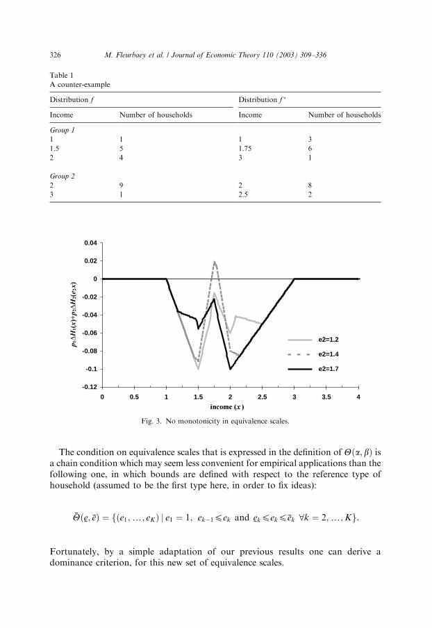
Example 4.1. Consider a population composed by two groups of needs with 10households in each group. Table 1 gives two distributions of income having the samemean.When the equivalence scale e2 is given, a necessary and sufficient condition for f to

dominate f � is6 p1DH1ðxÞ þ p2DH2ðe2xÞp0 8x:Fig. 3 provides the curve representing the function p1DH1ðxÞ þ p2DH2ðe2xÞ for

e2 ¼ 1:2; e2 ¼ 1:4 and e2 ¼ 1:7: f dominates f � if and only if the curve is alwaysbelow the horizontal axis. We remark that the dominance occurs when theequivalence scale is equal to 1.2 or 1.7, but not for 1.4.

5Using the HBAI income data and a parametric function of equivalence scales, Jenkins and Cowell [20]

obtain the same kind of result on inequality and poverty indices.6According to Ebert [14], checking this condition is equivalent to checking the Lorenz dominance on

equivalent incomes. Here, because the Lorenz curves are very close to each other, the stochastic dominance

condition gives a better visual illustration.


The condition on equivalence scales that is expressed in the definition of Yða; bÞ isa chain condition which may seem less convenient for empirical applications than thefollowing one, in which bounds are defined with respect to the reference type ofhousehold (assumed to be the first type here, in order to fix ideas):

%Yð%e; %eÞ ¼ fðe1;y; eKÞ j e1 ¼ 1; ek�1pek and

%ekpekp%ek 8k ¼ 2;y;Kg:

Fortunately, by a simple adaptation of our previous results one can derive adominance criterion, for this new set of equivalence scales.

Table 1

A counter-example

Distribution f Distribution f �

Income Number of households Income Number of households

Group 1

1 1 1 3

1.5 5 1.75 6

2 4 3 1

Group 2

2 9 2 8

3 1 2.5 2

-0.12

-0.1

-0.08

-0.06

-0.04

-0.02

0

0.02

0.04

0 0.5 1 1.5 2 2.5 3 3.5 4

e2=1.2

e2=1.4

e2=1.7

Fig. 3. No monotonicity in equivalence scales.


Theorem 4.2.

f DU2; %Yð%e;%eÞf

� ðAÞ

is equivalent toXK

k¼1pkDHkðxkÞp0 8ðxkÞk¼1;y;K ðBÞ

such that

x1A 0;max %s1;%s2

%e2;%s3

%e3;y;

%sK

%eK

� �� ;

0pxk�1pxkp%sk and%ekx1pxkp%ekx1 8k ¼ 2;y;K : ð23Þ

Proof. Sufficiency: Condition ð *BÞ implies ð *AÞ: The proof is exactly the same as theproof of sufficiency part of Theorem 4.1 given in footnote 4.

Necessity: ð *AÞ implies ð *BÞ: Suppose condition ð *BÞ is not satisfied. There exists areal number x; and a vector ðe1; e2;y; eKÞ such that e1 ¼ 1; and for all k ¼ 2;y;K ;

ek�1pek and%ekpekp%ek; such that

PKk¼1 pkDHkðekxÞ40: By a similar method as in

the necessity part of the proof of Theorem 3.1, one can find a function U in U2; suchthat DWU ;eo0; in contradiction with f DU2; %Yð

%e;%eÞf

�: &

An algorithm for implementing condition ð *BÞ is the following. DefineQKðx; yÞ ¼ max

zA½%eK x;%eK x�-½y;þN½

fpKDHKðzÞg;

Qkðx; yÞ ¼ maxzA½

%ekx;%ekx�-½y;þN½

fpkDHkðzÞ þ Qkþ1ðx; zÞg for k ¼ 2;y;K � 1:

Then a necessary and sufficient condition for f DU2; %Yða;bÞf� is

p1DH1ðxÞ þ Q2ðx; xÞp0 8xA 0;max %s1;%s2

%e2;%s3

%e3;y;

%sK

%eK

� �� :

The proof of this fact is similar to that of Proposition 3.2, and relies on the fact that

ð *CÞ is equivalent to

p1DH1ðxÞ þ maxx2A½

%e2x;%e2x�

p2DH2ðx2Þ þ maxx3A½

%e3x; %e3x�-½x2;þN½


p0

8xA 0;max %s1;%s2

%e2;%s3

%e3;y;

%sK

%eK

� �� and xkA½0; %sk� for k ¼ 2;y;K � 1:

5. Extension to the case where distribution of needs differ

When one wishes to make some intertemporal or inter-country comparisons ofwelfare, it is necessary to have a dominance criterion which allows to compare


distributions with different needs. Consider two income distributions f and f �;respectively, associated to the population shares vectors ðpkÞk¼1;y;K and ðp�

kÞk¼1;y;K :

First, rewrite expression (2) in this context:

DWV ¼XK

k¼1

Z %sk

0

D½pkfkðyÞ�Vðy; kÞ dy ð24Þ

with D½pkfkðyÞ� ¼ pkfkðyÞ � p�kf �

k ðyÞ:Assumptions U1–U4 introduced in Section 2 are not sufficient to obtain a similar

characterization to Theorem 3.1. Until now, the informational basis required by theaggregation process are captured by the cardinal unit-comparability invarianceaxiom defined by d’Aspremont and Gevers [11]. As noted by Atkinson andBourguignon [4], extending dominance results when the marginal distributions ofneeds differ requires a stronger invariance axiom known in the social choiceliterature as the full-comparability one, in which, additionally to the fact thatcomparing utility differences is meaningful, the utility levels can be compared. In theliterature, two kinds of assumptions have been proposed in this vein to extend theAtkinson–Bourguignon’s criterion. Before presenting our assumption, we discuss themerit of the proposals made by Jenkins and Lambert [21] and Moyes [23]. Theformer authors introduce a number %aX%sk 8k; which is interpreted as the maximumconceivable income (or income limit), and state that all households face the sameutility level for an income just equal to %a; i.e.

UJL: ( %V; Vð %a; kÞ ¼ %V 8k:

To make this assumption meaningful, one has to consider it jointly with the otherassumptions on utility functions and in particular U3B; stating that the larger theneed, the larger the marginal utility. Posed together, U3B and UJL capture two ideas.First, for a given income belonging to ½0; %aÞ; the smaller the need, the larger theutility level. Second, when the household income is very large the importance of thedifference in needs is negligible for a welfare analysis. Under UJL; social welfare isinvariant to transfers of population across groups of needs, at income level %a:Assumption UJL has been criticized by Moyes [23] on the ground it is too strong.

He proposes to consider only the first of the two previous ideas. Then, instead ofUJL; he makes the following assumption:

UM: Vðy; k � 1ÞXVðy; kÞ 8yA½0; %a�; 8kAf2;y;Kg:

Considering the family of utility functions satisfying U1, U2, U3B; UAB and UJL;Jenkins and Lambert show7 that a simple generalization of the dominance conditionof Atkinson and Bourguignon [3], recalled in Eq. (15), is valid in the case where the

7Notice that Jenkins and Lambert [21] only prove the sufficiency part of the result. The necessity part is

given by Chambaz and Maurin [9].


distribution of needs differ. This condition is written as

XK

k¼j

D½pkHkðxÞ�p0 8xA½0; %a�; 8j ¼ 1;y;K ; ð25Þ

where D½pkHkðxÞ� ¼R x

0

R y

0½pkfkðzÞ � p�

kf �k ðzÞ� dz dy:

Considering a larger family of utility functions leads to a more partial criterion ofdominance. Indeed, Moyes [23] proves that f dominates f � for the family of utilityfunctions satisfying assumptions U1, U2, U3B; UAB and UM if and only if

XK

k¼j

D½pkHkðxÞ�p0 8xA½0;maxð%s1;y; %sKÞ�; 8j ¼ 1;y;K ð26aÞ

and

XK

k¼j

½pk � p�k�p0 8j ¼ 2;y;K � 1: ð26bÞ

This last condition means that the proportion of needy people, evaluated in asequential way, is at least as great in the dominated configuration than in thedominating one. This condition restricts the set of income distributions to which thecomparative test can be performed, and therefore, passing from UJL to UM implies aloss of the discriminating power of the dominance criterion.Assumption UM implies a demographic condition like (26b) because the difference

between the utility levels for two different groups of needs can be arbitrarily large, sothat the proportion of more needy groups in the population becomes the onlyrelevant information in the comparison of income distributions. Symmetrically,assumption UJL means that the difference in utility vanishes totally for largeincomes. But it is worth noticing that Jenkins and Lambert’s criterion contains ademographic condition as well. This condition becomes more and more pregnant as

%a is large. At the limit, the demographic condition is Moyes’ one. More precisely, wecan state:

Remark 5.1. When %a goes to infinity, Jenkins’ and Lambert’s criterion boils down toMoyes’ one. Indeed, for xX%sk one can write

D½pkHkðxÞ� ¼D½pkHkð%skÞ� þ pk

Z x

%sk

FkðyÞ dy � p�k

Z x

%sk

F�k ðyÞ dy

¼ pk

Z %sk

0

ð%sk � yÞfkðyÞ dy � p�k

Z %sk

0

ð%sk � yÞf �k ðyÞ dy

þ ðpk � p�kÞðx � %skÞ

¼ pkð%sk � mfkÞ � p�

kð%sk � mf �kÞ þ ðpk � p�

kÞðx � %skÞ

¼ p�kmf �

k� pkmfk

þ ðpk � p�kÞx;


where mfkand mf �

krepresent the average incomes relative to fk and f �

k : Therefore, for

xXmaxð%s1;y; %sKÞ; condition (25) can be writtenXK

k¼j

D½pkHkðxÞ� ¼XK

k¼j

½p�kmf �

k� pkmfk

� þ xXK

k¼j

ðpk � p�kÞ 8j ¼ 1;y;K :

The functionPK

k¼j D½pkHkðxÞ� is monotone on the interval ½maxð%s1;y; %sKÞ;NÞ forall j: Then, checking the two following conditions is necessary and sufficient to verifyJenkins’ and Lambert’s criterion:XK

k¼j

D½pkHkðxÞ�p0 8xA½0;maxð%s1;y; %sKÞ�; 8j ¼ 1;y;K ; ð27aÞ

XK

k¼j

½p�kmf �

k� pkmfk

� þ %aXK

k¼j

ðpk � p�kÞp0 8j ¼ 2;y;K : ð27bÞ

When %a-N; a necessary and sufficient condition to verify (27b) is condition (26b).

Then, Moyes’ criterion corresponds to Jenkins’ and Lambert’s one whendifferences of utility between groups only vanish at the limit.Assuming UM or UJL in addition to the previous assumptions U1–U4 does not

raise a contradiction, but we prefer to consider an assumption which is more in tunewith the previous ones. Indeed, in view of our approach, one can interpret UJL asmeaning that differences of utility between groups of unequal needs may vanish, andUM as meaning that they are not bounded above. Considering that the differences ofutility due to differential needs are bounded,8 we propose a condition that issomehow intermediate between the two previous ones. The utility functions must besuch that there exist income levels for which differences of utility and differences ofmarginal utility disappear across groups. Like in Jenkins and Lambert, ourcondition is parameterized by an income limit which, here, is the income limit for areference group, w.l.o.g. group 1, a1: Let a1 be given. We introduce the followingassumption:

U5. There exist a2;y; aK ; %V and %V0 such that(i) Vðak; kÞ ¼ %V 8k;(ii) Vyðak; kÞ ¼ %V0 8k:

In contrast with UJL and UM the second part of U5 introduces a restriction onmarginal utility for income levels equal to the income limits ak: Composed withassumptions U2–U4, assumption U5(ii) allows to deduce that ðakÞk¼1;y;K satisfy

akp ak

ak�1pbk; k ¼ 2;y;K : In view of that restriction, assumption U5(i) states that

the differences in the utility level disappear across groups when the income level in

8Let us recall that the utility functions are defined on Rþ: Assumptions on utility functions beyond the

support have an impact about welfare comparisons performed over the support.


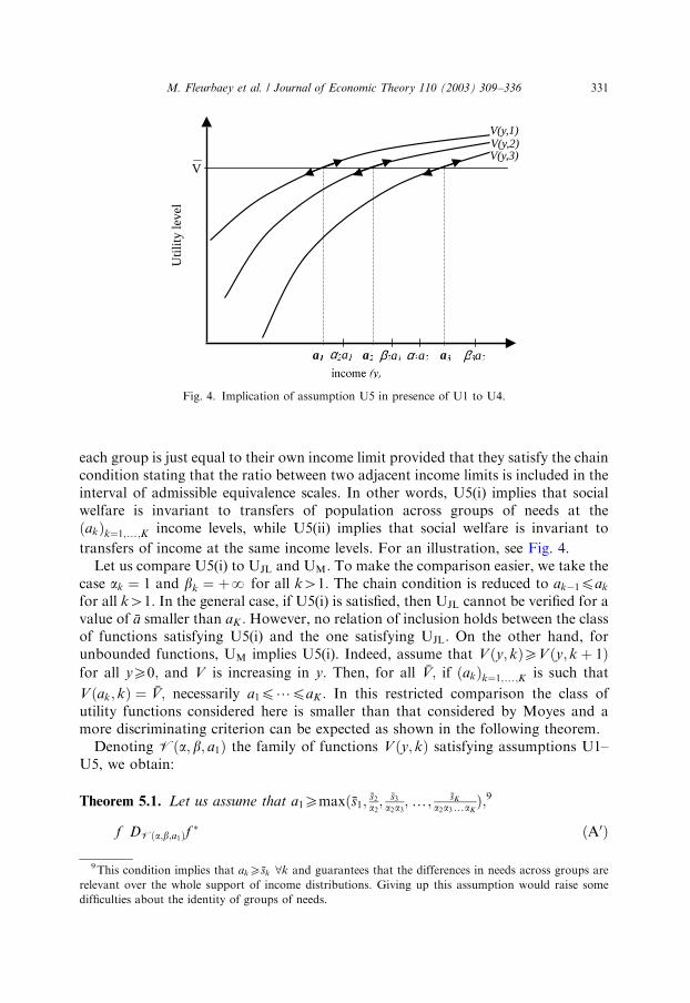
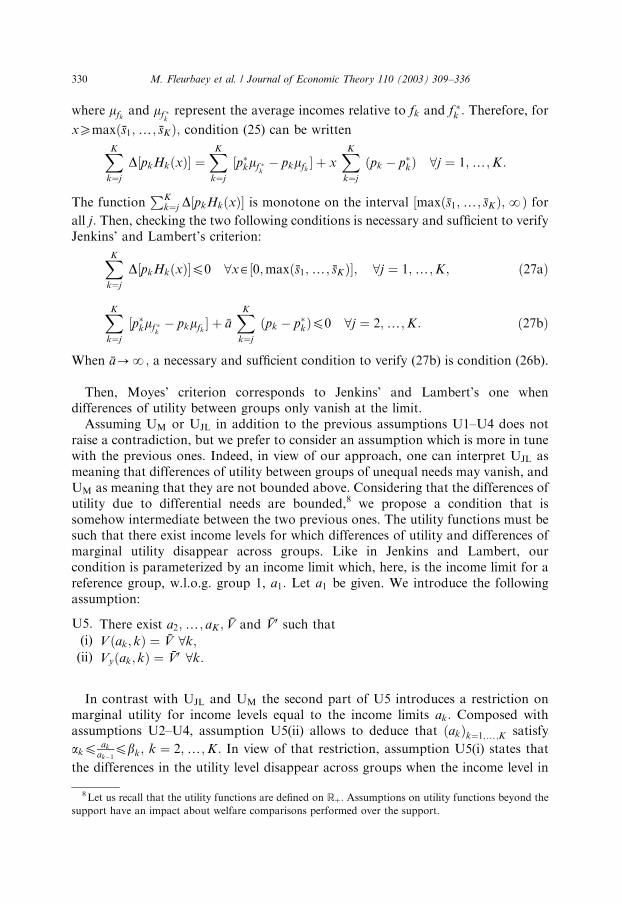
each group is just equal to their own income limit provided that they satisfy the chaincondition stating that the ratio between two adjacent income limits is included in theinterval of admissible equivalence scales. In other words, U5(i) implies that socialwelfare is invariant to transfers of population across groups of needs at theðakÞk¼1;y;K income levels, while U5(ii) implies that social welfare is invariant to

transfers of income at the same income levels. For an illustration, see Fig. 4.Let us compare U5(i) to UJL and UM: To make the comparison easier, we take the

case ak ¼ 1 and bk ¼ þN for all k41: The chain condition is reduced to ak�1pak

for all k41: In the general case, if U5(i) is satisfied, then UJL cannot be verified for avalue of %a smaller than aK : However, no relation of inclusion holds between the classof functions satisfying U5(i) and the one satisfying UJL: On the other hand, forunbounded functions, UM implies U5(i). Indeed, assume that Vðy; kÞXVðy; k þ 1Þfor all yX0; and V is increasing in y: Then, for all %V; if ðakÞk¼1;y;K is such that

Vðak; kÞ ¼ %V; necessarily a1p?paK : In this restricted comparison the class ofutility functions considered here is smaller than that considered by Moyes and amore discriminating criterion can be expected as shown in the following theorem.Denoting Vða; b; a1Þ the family of functions Vðy; kÞ satisfying assumptions U1–

U5, we obtain:

Theorem 5.1. Let us assume that a1Xmaxð%s1; %s2a2;%s3

a2a3;y; %sK

a2a3yaKÞ;9

f DVða;b;a1Þf� ðA0Þ

a α a β a

VU

tility

leve

l

a a β aα a

V(y,1)V(y,2)V(y,3)

Fig. 4. Implication of assumption U5 in presence of U1 to U4.

9This condition implies that akX%sk 8k and guarantees that the differences in needs across groups are

relevant over the whole support of income distributions. Giving up this assumption would raise some

difficulties about the identity of groups of needs.


is equivalent to

XK

k¼1D½pkHkðxkÞ�p0 8ðxkÞk¼1;y;K ðB0Þ

such that

0px1pa1;

and

akxk�1pxkpbkxk�1 8k ¼ 2;y;K :

Proof. This proof is similar to Theorem 3.1.

Sufficiency: Condition ðB0Þ implies ðA0Þ: We have to modify the functions Vnðy; kÞin comparison to the proof of Theorem 3.1. Let us take

V nðy; kÞ ¼ Vðy; kÞ þ ak

nlog

y

ak

þ 1

� �� ak

nlogð2Þ: ð28Þ

Since D½pkfkðyÞ� ¼ 0 8yX%sk and akX%sk; 8k; expression (24) can be written as

DWV ¼XK

k¼1

Z ak

0

D½pkfkðyÞ�Vðy; kÞ dy:

When V n is considered, integrating by parts and using assumption U5(i) give

DW nV ¼ %V

XK

k¼1ðpk � p�

kÞ �XK

k¼1

Z ak

0

V ny ðy; kÞD½pkFkðyÞ� dy:

BecausePK

k¼1 pk ¼PK

k¼1 p�k ¼ 1; it follows that

DWV ¼ �XK

k¼1

Z ak

0

V ny ðy; kÞD½pkFkðyÞ� dy:

In the remaining of the proof, it is enough to replace pkDFkðyÞ by D½pkFkðyÞ�; whichis equal to

R y

0 ½pkfkðzÞ � p�kf �

k ðzÞ� dz; and to take bk ¼ ak 8k; with

a1Xmaxð%s1; %s2a2;%s3

a2a3;y; %sK

a2a3yaKÞ: Notice that the condition ak ¼ jkðak�1Þ is now

implied by assumption U5(ii).Hence, the following condition emerges (instead of condition (9)):

XK

k¼1D½pkHkðjk3jk�13?3j2ðyÞÞ�p0; for all yA½0; a1�;

and all functions jk such that akypjkðyÞpbky 8k ¼ 2;y;K :We end the proof in a similar way, noting that a difference with Theorem 3.1

comes from the fact that we cannot avoid to check the conditionPKk¼1 D½pkHkðxkÞ�p0; for x1Xmaxð%s1; %s2b2;

%s3b2b3

;y; %sK

b2b3ybKÞ: Indeed, the functions

D½pkHk� are not constant beyond %sk:


Necessity: Condition ðA0Þ implies ðB0Þ: Suppose that f DVða;b;a1Þf� and there exists

a K-vector ðe1; e2;y; eKÞ such that

0pekpak for all k ¼ 1;y;K ; ð29aÞ

akek�1pekpbkek�1 for all k ¼ 2;y;K ; ð29bÞ

and

XK

k¼1D½pkHkðekÞ�40: ð29cÞ

The proof is exactly the same than Theorem 3.1. To verify U1–U5, we consider thefunction U0ðxÞ which satisfies expression (12) and is equal to 0 for xXe: Settingbk ¼ ak; the property ekpbk is now satisfied by assumption (29a). &

As a byproduct, this result provides an extension of Bourguignon’s criterion to thecase of different distributions of needs.Contrary to the case where the population composition does not vary, the

functions D½pkHk� are not constant beyond the upper bound of the support of Dfk:Consequently, the dominance criterion defined in Theorem 5.1 is dependent on thevalue of a1; which can be interpreted as the income limit chosen by the decisionmaker for the reference group. This may deserve a more detailed explanation.

As for the Jenkins and Lambert’s criterion, condition ðB0Þ can be rewritten as the

sum of two terms when x1Xmaxð%s1; %s2a2;%s3

a2a3;y; %sK

a2a3yaKÞ:

XK

k¼1D½pkHkðxkÞ� ¼

XK

k¼1½p�

kmf �k� pkmfk

� þ x1

XK

k¼1ðpk � p�

kÞYk

l¼1gl

with g1 ¼ 1 and alpglpbl ; l ¼ 2;y;K: The gl ’s are nothing else that the incomeratio of individuals belonging to two adjacent groups.One can see that, for a given vector ðgkÞk¼1;y;K ; the above function is monotone

on the interval ½maxð%s1; %s2a2;%s3

a2a3;y; %sK

a2a3yaKÞ;NÞ: Therefore, checking our criterion is

equivalent to checking the two following conditions.

XK

k¼1D½pkHkðxkÞ�p0 8ðxkÞk¼1;y;K ð30aÞ

such that

x1pmax %s1;%s2

a2;

%s3

a2a3;y;

%sK

a2a3yaK

� �and akxk�1pxkpbkxk�1

8k ¼ 2;y;K ;

XK

k¼1½p�

kmf �k� pkmfk

� þ a1XK

k¼1ðpk � p�

kÞYk

l¼1glp0 8ðglÞl¼1;y;K ð30bÞ


such that

g1 ¼ 1 and alpglpbl 8l ¼ 2;y;K :

The first term only depends on the distributions of income, whereas the secondterm is purely demographic, and overrides the first one when the a1 is large enough.This can be understood by the fact that when the a1 grows large, assumption U5ðiÞ is

less and less restrictive about the differences in utility levels between groups overvalues of incomes within the support. In application, the most discriminatingcriterion corresponds to minimal value of income limit for the reference group, that

is maxð%s1; %s2a2;%s3

a2a3;y; %sK

a2a3yaKÞ:

In the limit case, when a1 goes to infinity, condition (30b) is reduced to thefollowing one:

XK

k¼1ðpk � p�

kÞYk

l¼1glp0 8ðglÞl¼1;y;K ð31Þ

such that

g1 ¼ 1 and alpglpbl 8l ¼ 2;y;K :

Comparing with the Moyes’ condition (26b) is only meaningful in the case whereUM implies U5(i) (ak ¼ 1 and bk ¼ þN for all k41). Then, in this very particularcase, it can be established that the above condition is equivalent to Moyes’one.For applications, note that the algorithm presented in Theorem 3.2 is immediately

adapted to the present setting, by replacing pkDHk by D½pkHk�:

6. Conclusion

The paper has considered the problem of comparing income distributions forheterogeneous populations. Following Atkinson and Bourguignon [3], we havedivided the population in different groups of needs and evaluated the social welfarewith a utilitarian function. By introducing principles which bound the socialmarginal value of income for a group of need with respect to that value for adifferent group of need, we have found an implementable condition of dominancewhich allows to rank more distributions than the Bourguignon criteria [6].Furthermore, we have shown that this condition amounts to applying the one-dimensional dominance criterion on equivalent income distributions by consideringa social welfare function weighted by equivalence scales, these not being given butbelonging to intervals. Finally, we have extended our results to the case wheredistributions of needs differ between the two populations being compared. Inparticular in tune with our framework, we make use of a condition which bounds thedifference of utility levels across groups.We have supposed in the paper that there is no ambiguity about the ranking of

groups with respect to their needs. But in applications, if there is a doubt about theranking, one only has to perform the dominance analysis for all potential rankings.


Our criterion degenerates to Bourguignon’s one [6] when we consider unboundedequivalence scales. A further investigation would be to start again all the analysis ofthis paper in order to have the dominance criterion obtained degenerating toAtkinson and Bourguignon’s one [3] at the limit. But it cannot be done simply bycombining U1–U4 and UAB because the family of utility functions satisfying theseassumptions is degenerate and has equal marginal utilities across groups of needs.10

In a companion paper [16], we show that the discriminating power of our criterionis much greater than both Bourguignon’s criterion and Atkinson’s and Bour-guignon’s one, on actual data about the French income distribution.

Acknowledgments

We thank M. Scarsini, U. Ebert, P. Moyes and an anonymous referee forcomments, and participants in conferences in Paris and Vancouver. We remain solelyresponsible for the shortcomings of this paper.

References

[1] T.M. Apostol, Mathematical Analysis, Addison-Wesley Publishing, Reading, MA, 1974.

[2] A.B. Atkinson, On the measurement of inequality, J. Econom. Theory 2 (1970) 244–263.

[3] A.B. Atkinson, F. Bourguignon, Income distribution and differences in needs, in: G.R. Feiwel (Ed.),

Arrow and the Foundation of the Theory of Economic Policy, Macmillan, London, 1987.

[4] A.B. Atkinson, F. Bourguignon, Income distribution and economics, in: A.B. Atkinson, F.

Bourguignon (Eds.), Handbook of Income Distribution, North-Holland, Amsterdam, 2000.

[5] R. Blundell, A. Lewbel, The information content of equivalence scales, J. Econometrics 50 (1991)

49–68.

[6] F. Bourguignon, Family size and social utility. Income distribution dominance criteria, J.

Econometrics 42 (1989) 67–80.

[7] B. Bradbury, Measuring poverty changes with bounded equivalence scales: Australia in the 1980s,

Economica 64 (1997) 245–264.

[8] B.L. Buhmann, L. Rainwater, G. Schmaus, T.M. Smeeding, Equivalence scales, well-being,

inequality, and poverty: sensitivity estimates across ten countries using the Luxembourg income

study (LIS) database, Rev. Income Wealth 34 (1989) 115–142.

[9] C. Chambaz, E. Maurin, Atkinson and Bourguignon’s dominance criteria: extended and applied to

the measurement of poverty in France, Rev. Income Wealth 44 (1998) 497–513.

[10] F.A. Cowell, M. Mercader-Prats, Equivalence scales and inequality, in: J. Silber (Ed.), Income

Inequality Measurement: from Theory to Practice, Kluwer, Dewenter, 1999.

[11] C. d’Aspremont, L. Gevers, Equity and the informational basis of collective choice, Rev. Econom.

Stud. 44 (1977) 199–210.

[12] U. Ebert, Income inequality and differences in household size, Math. Soc. Sci. 30 (1995) 37–55.

[13] U. Ebert, Social welfare when needs differ: an axiomatic approach, Economica 64 (1997) 233–344.

[14] U. Ebert, Using equivalence income of equivalent adults to rank income distributions, Soc. Choice

Welfare 16 (1999) 233–258.

10U3 and U4 imply that marginal utilities are equal across groups at y ¼ 0; while UAB requires that the

excess of marginal utility due to higher needs decreases with y:


[15] U. Ebert, Sequential generalized Lorenz dominance and transfer principles, Bull. Econom. Res. 52

(2000) 113–123.

[16] M. Fleurbaey, C. Hagnere, A. Trannoy, Mesure des effets redistributifs d’une reforme des minima

sociaux a l’aide d’un nouveau critere de dominance, Revue Econom. 53 (2002) 1205–1234.

[17] J.E. Foster, A.F. Shorrocks, Poverty orderings and welfare dominance, Soc. Choice Welfare 5 (1988)

179–198.

[18] P. Glewwe, Household equivalence scales and the measurement of inequality: transfers from the poor

to the rich could decrease inequality, J. Public Econom. 44 (1991) 211–216.

[19] S.P. Jenkins, Income inequality and living standards: changes in the 1970s and 1980s, Fiscal Stud. 12

(1991) 1–28.

[20] S.P. Jenkins, F.A. Cowell, Parametric equivalence scales and scale relativities, Econom. J. 104 (1994)

891–900.

[21] S.P. Jenkins, P.J. Lambert, Ranking income distributions when needs differ, Rev. Income Wealth 39

(1993) 337–356.

[22] N.C. Kakwani, Analysing Redistribution Policies: a Study using Australian Data, Cambridge

University Press, Cambridge, 1986.

[23] P. Moyes, Comparisons of heterogeneous distributions and dominance criteria, Economie et

Prevision 138–139 (1999) 125–146 (in French).

[24] E.A. Ok, P.J. Lambert, An evaluating social welfare by sequential generalized Lorenz dominance,

Econom. Letters 63 (1999) 39–44.

[25] R. Pollak, T. Wales, Welfare comparisons and equivalence scales, Amer. Econom. Rev. 69 (1979)

216–222.

[26] A.F. Shorrocks, Ranking income distributions, Economica 50 (1983) 1–17.

[27] A.F. Shorrocks, Inequality and welfare evaluation of heterogeneous income distributions, Discussion

Paper No. 447, Department of Economics, University of Essex, 1995.


welfarecomparisonswithbounded...

Documents