well-conditioned collocation schemes and new triangular spectral-element methods
TRANSCRIPT

Spectral methods Well-conditioned collocation New TSEM Further studies
Well-Conditioned Collocation Schemes and
New Triangular Spectral-Element Methods
Michael Daniel V. [email protected]
supervised by Li-Lian Wang
Nanyang Technological University
29 April 2014

Spectral methods Well-conditioned collocation New TSEM Further studies
Spectral methods
Background and historyPolynomial representation
Well-conditioned collocation
PreliminariesBirkhoff interpolation methodExtensions
New TSEM
PreliminariesNew transformImplementation
Further studies
CollocationTSEMFurther reading

Spectral methods Well-conditioned collocation New TSEM Further studies
Numerical solution of differential equations
Given f ∈ L2(Ω), g ∈ L2(∂Ω), find u such that
Lu = f in Ω differential operator,
Bu = g on ∂Ω boundary conditions.
f and g are given as data on predetermined points in thedomain Ω and on the boundary ∂Ω, respectively.
This allows for the determination of a numerical solution uN ,which can be computed in a few ways.

Spectral methods Well-conditioned collocation New TSEM Further studies
Lagrange interpolation
Given data (xi, yi), 0 ≤ i ≤ N , with pairwise distinct xi ∈ R,the Lagrange interpolation of the data is given as p ∈ PN
satisfyingp(xi) = yi for 0 ≤ i ≤ N,
computed by
p(x) =N∑
i=0
yiLi(x) where Li(x) =
0≤j≤N∏
i 6=j
x− xjxi − xj
.
Li is the Lagrange interpolation basis at the points xi,also as the nodal basis, as each function is 1 on one node and 0on the others, Li(xj) = δij .

Spectral methods Well-conditioned collocation New TSEM Further studies
Lagrange interpolation at quadrature points
If the nodes are Gauss-type quadrature points, with associatedweights ωi, then the Lagrange interpolation polynomials aregiven as
Li(x) =ωi
2
N∑
k=0
(2k + 1)Pk(xi)Pk(x)
for Legendre-Gauss-type points, and
Li(x) =ωi
π+
2ωi
π
N∑
k=1
Tk(xi)Tk(x)
for Chebyshev-Gauss-type points.
Spectral methods Well-conditioned collocation New TSEM Further studies
Collocation scheme
Given nodes ~xi, values f(~xi), g(~xi), 0 ≤ i ≤ N , find uN suchthat
LuN (~xi) = f(~xi) for each ~xi ∈ Ω;
BuN (~xi) = g(~xi) for each ~xi ∈ ∂Ω.
These equations form a linear system A~u = ~f , where theunknown is ~u = (uN (x0), . . . , uN (xN ))t.
If the components of the nodes are, depending on Ω and B,Gauss-Radau or Gauss-Lobatto points, the nodes are spectral
collocation points.

Spectral methods Well-conditioned collocation New TSEM Further studies
Second-order BVP with Lagrange interpolationGiven I = (−1, 1), r, s, f ∈ C(I) and u±, find u such that
−u′′ + ru′ + su = f in I; u(±1) = u±.
For nodes −1 = x0 < x1 < · · · < xN−1 < xN = 1, let
uN (x) =N∑
i=0
uiLi(x),
where Li is the nodal basis on xi. The collocation schemeis, for 0 < i < N ,
−N−1∑
k=1
ukL′′k(xi) + r(xi)
N−1∑
k=1
ukL′k(xi) + s(xi)ui
=f(xi) + u−(L′′0(xi)− r(xi)L
′0(xi)) + u+(L
′′N (xi)− r(xi)L
′N (xi)).

Spectral methods Well-conditioned collocation New TSEM Further studies
Linear system from Lagrange interpolation
When uN (x) =∑N
i=0 uiLi(x), with Li the nodal basis on xi:
(−D(2)in +ΛrD
(1)in +Λs)~u = ~f+u−(~d
(2)0 −Λr
~d(1)0 )+u+(~d
(2)N −Λr
~d(1)N ),
where
D(m)in = [L
(m)j (xi)]
N−1i,j=1,m = 1, 2 ~u = (u1, . . . , uN−1)
t,
Λφ = diag(φ(x1), · · · , φ(xN−1)), φ = r, s, ~f = (f(x1), . . . , f(xN−1))t,
~d(m)k = (L
(m)k (x1), . . . , L
(m)k (xN−1))
t, m = 1, 2, k = 0, N.
For spectral collocation points, D(m)in and ~d
(m)k , m = 1, 2,
k = 0, N , are computed accurately and efficiently.

Spectral methods Well-conditioned collocation New TSEM Further studies
Spectral collocation using Lagrange interpolationConsider
u′′(x)−(1+sinx)u′(x)+exu(x) = f(x), x ∈ (−1, 1); u(±1) = u±,
with f ∈ C1(I) and the exact solution u ∈ C3(I), given by
u(x) =
cosh(x+ 1)− x2/2− x, −1 ≤ x < 0,
cosh(x+ 1)− cosh(x)− x+ 1, 0 ≤ x ≤ 1.
101
102
103
10−14
10−12
10−10
10−8
10−6
10−4
10−2
N
BCOLLCOLPLCOL
101
102
103
10−14
10−12
10−10
10−8
10−6
10−4
10−2
N
BCOLLCOLPLCOL

Spectral methods Well-conditioned collocation New TSEM Further studies
Motivations and goals
Generate a collocation scheme that is
• Well-conditioned: condition number for Lagrangeinterpolation collocation for second-order BVP is O(N4)
• Stably, efficiently, accurately computed: as in Lagrangeinterpolation collocation
Previous methods use preconditioning or spectral integrationto generate systems with better condition numbers, but stilldependent on N

Spectral methods Well-conditioned collocation New TSEM Further studies
Well-conditioned collocation scheme
Generate a well-conditioned collocation scheme based on adifferent interpolation basis
• Uses integration on nodal functions to generate systemswith condition number independent of N
• Generates an optimal preconditioner—inverts thedifferential matrix of highest order
• Computed accurately, stably and efficiently—based onslowly-decaying coefficient matrices
The new interpolation basis has to be carefully verified andcomputed, as it does not always exist, and that modifications
may be needed to ensure the collocation scheme iswell-conditioned.

Spectral methods Well-conditioned collocation New TSEM Further studies
Birkhoff interpolation for second-order BVP
Given data (xi, y2i ), 0 < i < N , y0 and yN , with−1 = x0 < x1 < · · · < xN−1 < xN = 1, the Birkhoff
interpolation of the data is given as p ∈ PN satisfying
p(−1) = y0; p′′(xi) = y2i for 0 < i < N ; p(1) = yN
computed by p(x) = y0B0(x)+∑N−1
i=1 y2iBi(x)+ yNBN (x) where
B0(−1) = 1; B′′0 (xi) = 0, 0 < i < N ; B0(1) = 0;
Bj(−1) = 0; B′′j (xi) = δij , 0 < i < N ; Bj(1) = 0, 0 < j < N ;
BN (−1) = 0; B′′N (xi) = 0, 0 < i < N ; BN (1) = 1.
Bi is the Birkhoff interpolation basis at the points xi.

Spectral methods Well-conditioned collocation New TSEM Further studies
Birkhoff interpolation for second-order BVP
Given data (xi, y2i ), 0 < i < N , y0 and yN , with−1 = x0 < x1 < · · · < xN−1 < xN = 1, the Birkhoff
interpolation of the data is given as p ∈ PN satisfying
p(−1) = y0; p′′(xi) = y2i for 0 < i < N ; p(1) = yN
computed by p(x) = y0B0(x)+∑N−1
i=1 y2iBi(x)+ yNBN (x) where
B0(x) = (1− x)/2;
Bj(−1) = 0; B′′j (xi) = δij , 0 < i < N ; Bj(1) = 0, 0 < j < N ;
B0(x) = (1 + x)/2.
Bi is the Birkhoff interpolation basis at the points xi.
Spectral methods Well-conditioned collocation New TSEM Further studies
Stable anti-differentiation on orthogonal polynomials
Define the following antiderivatives:
∂(−1)x P0(x) =
1 + x
2; ∂(−1)
x Pk(x) =Pk+1(x)− Pk−1(x)
2k + 1, k > 0;
∂(−1)x T0(x) =
1 + x
2; ∂(−1)
x T1(x) =x2 − 1
2;
∂(−1)x Tk(x) =
Tk+1(x)
k + 1− Tk−1(x)
k − 1− 2(−1)k
k2 − 1, k > 1;
and ∂(−[m+1])x φ = ∂
(−1)x [∂
(−m)x φ]. Then
∫ x
−1φ(t) dt = ∂(−1)
x φ(x).
Note that ∂(−1)x Pk(−1) = ∂
(−1)x Tk(−1) = 0, k ≥ 0, but
∂(−1)x Pk(1) = 0 for k > 0 and ∂
(−1)x Tk(1) = 0, for odd k > 0.

Spectral methods Well-conditioned collocation New TSEM Further studies
Birkhoff interpolation for spectral collocation points
For Gauss-Lobatto quadrature points and weights (xi, ωi), theassociated Birkhoff interpolation polynomials Bi, 0 < i < N ,follow from
B′′i (x) =
ωi
2
N−2∑
k=0
(2k + 1)[Pk(xi)− PN−mN−k(xi)]Pk(x)
for Legendre-Gauss-Lobatto points, and
B′′i (x) =
ωi
π(1−TN−mN
(xi))+2ωi
π
N−2∑
k=1
[Tk(xi)−TN−mN−k(xi)]Tk(x)
for Chebyshev-Gauss-Lobatto points, where mj = j mod 2.

Spectral methods Well-conditioned collocation New TSEM Further studies
Birkhoff interpolation for spectral collocation points
For Gauss-Lobatto quadrature points and weights (xi, ωi), theassociated Birkhoff interpolation polynomials Bi, 0 < i < N ,are given by
Bi(x) =ωi
2
N−2∑
k=0
(2k + 1)[Pk(xi)− PN−mN−k(xi)]∂
(−2)x Pk(x)
− (1 + x)ωi
4[1− PN−mN
(xi)]∂(−2)x P0(1)
− (1 + x)3ωi
4[xi − PN−mN−1
(xi)]∂(−2)x P1(1)
for Legendre-Gauss-Lobatto points, where mj = j mod 2.

Spectral methods Well-conditioned collocation New TSEM Further studies
Birkhoff interpolation for spectral collocation points
For Gauss-Lobatto quadrature points and weights (xi, ωi), theassociated Birkhoff interpolation polynomials Bi, 0 < i < N ,are given by
Bi(x) =2ωi
π
N−2∑
k=1
[Tk(xi)− TN−mN−k(xi)]∂
(−2)x Tk(x)
− (1 + x)ωi
π
N−2∑
k=1
[Tk(xi)− TN−mN−k(xi)]∂
(−2)x Tk(1)
+ωi
2π(1− TN−mN
(xi))[2∂(−2)x (x)− ∂(−2)
x (1)(1 + x)]
for Chebyshev-Gauss-Lobatto points, where mj = j mod 2.

Spectral methods Well-conditioned collocation New TSEM Further studies
Collocation scheme using Birkhoff interpolationGiven I = (−1, 1), b, c, f ∈ C(I), γ > 0 and u±, find u such that
−u′′ + bu′ + cu = f in I; u(±1) = u±.
For nodes −1 = x0 < x1 < · · · < xN−1 < xN = 1, let
uN (x) =N∑
i=0
viBi(x),
where Bi is Birkhoff interpolation basis on xi. Thecollocation scheme is, for 0 < i < N ,
− vi + b(xi)
N−1∑
k=1
vkB′k(xi) + c(xi)
N−1∑
k=1
vkBk(xi)
=f(xi) +u−(b(xi)− c(xi)(1− xi))− u+(b(xi) + c(xi)(1 + xi))
2.

Spectral methods Well-conditioned collocation New TSEM Further studies
Linear system from Birkhoff interpolation
When uN (x) =∑N
i=0 viBi(x), with Bi the Birkhoffinterpolation basis on xi:
(−IN−1+ΛbB(1)in +ΛcB
(0)in )~v = ~f+
(u− − u+)Λb~1−Λc(u−~x− + u+~x+)
2,
where
B(m)in = [B
(m)j (xi)]
N−1i,j=1,m = 0, 1 ~v = (v1, . . . , vN−1)
t,
Λφ = diag(φ(x1), · · · , φ(xN−1)), φ = b, c, ~f = (f(x1), . . . , f(xN−1))t,
~1 = (1, . . . , 1)t, ~x± = ~1± (x1, . . . , xN−1)t.
For spectral collocation points, B(m)in , m = 0, 1, are computed
accurately and efficiently. Solution: ~u = u−~x− +B(0)in ~v+ u+~x+.

Spectral methods Well-conditioned collocation New TSEM Further studies
Second-order BVP with Birkhoff interpolation
Consider the example
u′′(x)−(1+sinx)u′(x)+exu(x) = f(x), x ∈ (−1, 1); u(±1) = u±,
with the exact solution u(x) = e(x2−1)/2. For Legendre spectral
collocation points,
NLagrange Birkhoff Preconditioned Lagrange
Cond.# Error iters Cond.# Error iters Cond.# Error iters
64 3.97e+05 3.82e-14 286 6.36 5.55e-16 10 2.86 1.67e-15 8
128 6.23e+06 4.42e-13 1251 6.46 1.11e-15 10 2.86 2.44e-15 8
256 9.91e+07 3.95e-13 6988 6.51 1.11e-15 11 2.86 2.55e-15 8
512 1.58e+09 1.02e-11 9457 6.54 1.89e-15 11 2.86 4.77e-15 8
1024 2.52e+10 6.58e-12 9697 6.55 3.44e-15 11 2.86 1.15e-14 9
The Lagrange linear system is preconditioned with
B(0)in = [D
(2)in ]−1. BiCGSTAB iteration is used (initial: ~0).

Spectral methods Well-conditioned collocation New TSEM Further studies
Second-order BVP with Birkhoff interpolation
Consider the example
u′′(x)−(1+sinx)u′(x)+exu(x) = f(x), x ∈ (−1, 1); u(±1) = u±,
with the exact solution u(x) = e(x2−1)/2. For Chebyshev
spectral collocation points,
NLagrange Birkhoff Preconditioned Lagrange
Cond.# Error iters Cond.# Error iters Cond.# Error iters
64 7.23e+05 8.38e-14 285 6.43 7.77e-16 10 2.86 1.44e-15 8
128 1.16e+07 2.87e-13 1304 6.50 7.77e-16 10 2.86 4.22e-15 8
256 1.85e+08 9.74e-13 5868 6.53 1.22e-15 11 2.86 6.55e-15 8
512 2.96e+09 4.51e-12 9987 6.55 1.78e-15 11 2.86 3.44e-15 8
1024 4.73e+10 1.27e-11 9938 6.56 3.77e-15 11 2.86 6.00e-15 9
The Lagrange linear system is preconditioned with
B(0)in = [D
(2)in ]−1. BiCGSTAB iteration is used (initial: ~0).

Spectral methods Well-conditioned collocation New TSEM Further studies
Second-order BVP with mixed boundary using
Birkhoff interpolation
Given a second-order BVP with the mixed-boundary conditions
u(−1)− u′(−1) = c−, u(1) + u′(1) = c+,
where c± are given. Compare condition numbers for Lagrangeinterpolation (LCOL) and Birkhoff interpolation (BCOL):
N−u′′ + u = f u′′ + u′ + u = f
Chebyshev Legendre Chebyshev LegendreBCOL LCOL BCOL LCOL BCOL LCOL BCOL LCOL
32 2.42 1.21e+05 2.45 6.66e+04 2.61 1.43e+05 2.61 7.87e+04
64 2.43 2.65e+06 2.45 1.41e+06 2.63 3.15e+06 2.63 1.68e+06
128 2.44 5.88e+07 2.45 3.09e+07 2.64 7.04e+07 2.64 3.70e+07
256 2.44 1.32e+09 2.45 6.88e+08 2.64 1.58e+09 2.64 8.26e+08
512 2.44 2.97e+10 2.44 1.54e+10 2.65 3.57e+10 2.65 1.86e+10
1024 2.44 6.71e+11 2.44 3.48e+11 2.65 8.08e+11 2.65 4.19e+11
Spectral methods Well-conditioned collocation New TSEM Further studies
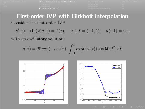
First-order IVP with Birkhoff interpolationConsider the first-order IVP
u′(x)− sin(x)u(x) = f(x), x ∈ I = (−1, 1); u(−1) = u−,
with an oscillatory solution:
u(x) = 20 exp(− cos(x))
∫ x
−1exp(cos(t)) sin(500t2) dt.
−1 −0.5 0 0.5 1−0.5
0
0.5
1
1.5
2
x400 450 500 550 600 650 700 750
10−14
10−12
10−10
10−8
10−6
10−4
10−2
100
N
BCOLLCOL

Spectral methods Well-conditioned collocation New TSEM Further studies
Third-order BVP with Birkhoff interpolation
Consider the following problem: for x ∈ I = (−1, 1),
−u′′′(x) + r(x)u′′(x) + s(x)u′(x) + t(x)u(x) = f(x);
u(±1) = u±, u′(1) = u1,
where r, s, t and f are given continuous functions on I, and u−,u+ and u1 are given constants.
The condition numbers of the coefficient matrices for CGLpoints are tabulated.
N r ≡ s ≡ 0, t ≡ 1 r ≡ 0, s ≡ t ≡ 1 s ≡ 0, r ≡ t ≡ 1 r ≡ s ≡ t ≡ 1
128 1.16 1.56 2.22 1.80
256 1.16 1.56 2.22 1.80
512 1.16 1.56 2.23 1.80
1024 1.16 1.56 2.23 1.80
Spectral methods Well-conditioned collocation New TSEM Further studies
Third-order Korteweg-de VriesConsider the third-order Korteweg-de Vries (KdV) equation:
∂tu+ u∂xu+ ∂3xu = 0, x ∈ (−∞,∞), t > 0; u(x, 0) = u0(x),
with the exact soliton solution
u(x, t) = 12κ2sech2(κ(x− 4κ2t− x0)),
where κ and x0 are constants. Let τ be the time step size. Usethe Crank-Nicolson leap-frog scheme in time and the newcollocation method in space: find uk+1
N ∈ PN+1 such that for0 < j < N ,
uk+1N (Lxj)− uk−1
N (Lxj)
2τ+ ∂3x
(uk+1N + uk−1
N
2
)(Lxj)
=− ∂xukN (Lxj)u
kN (Lxj);
ukN (±L) = ∂xukN (L) = 0, k ≥ 0.

Spectral methods Well-conditioned collocation New TSEM Further studies
Third-order KdV results
Let κ = 0.3, x0 = −20, L = 50 and τ = 0.001.
80 90 100 110 120 130 140 150 16010
−7
10−6
10−5
10−4
10−3
10−2
10−1
N
t = 1t = 50
On left, the numerical evolution of the solution with t ≤ 50 andN = 160. On right, the maximum point-wise errors for variousN at t = 1, 50.

Spectral methods Well-conditioned collocation New TSEM Further studies
Fifth-order BVP with Birkhoff interpolationConsider the fifth-order problem:u(5)(x) + a(x)u′(x) + b(x)u(x) = f(x), x ∈ I = (−1, 1);
u(±1) = u′(±1) = u′′(1) = 0,
where a, b and f are given continuous functions on I.
Compare the generalized Lagrange interpolation p ∈ PN+3
satisfying, for u ∈ C5(I), u(±1) = u′(±1) = u′′(1) = 0,
p(yj) = u(yj), 0 < j < N ; p(±1) = p′(±1) = p′′(1) = 0,
where yjN−1j=1 are zeros of the Jacobi polynomial J
(3,2)N−1(x),
computed by p(x) =∑N−1
j=1 u(xj)Lj(x) where
Lj(x) =J(3,2)N−1(x)
(x− xj)∂xJ(3,2)N−1(xj)
(1− x)3(1 + x)2
(1− xj)3(1 + xj)2.

Spectral methods Well-conditioned collocation New TSEM Further studies
Fifth-order BVP resultsSolving by the three collocation schemesu(5)(x) + sin(10x)u′(x) + xu(x) = f(x), x ∈ I = (−1, 1);
u(±1) = u′(±1) = u′′(1) = 0, with solution u(x) = sin3(πx).
20 40 60 80 100 120 140 160 180 20010
−14
10−10
10−6
10−2
102
N
BCOLLCOLSCOL
Spectral methods Well-conditioned collocation New TSEM Further studies
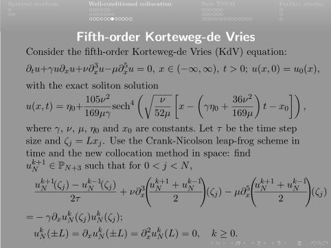
Fifth-order Korteweg-de VriesConsider the fifth-order Korteweg-de Vries (KdV) equation:
∂tu+γu∂xu+ν∂3xu−µ∂5xu = 0, x ∈ (−∞,∞), t > 0; u(x, 0) = u0(x),
with the exact soliton solution
u(x, t) = η0+105ν2
169µγsech4
(√ν
52µ
[x−
(γη0 +
36ν2
169µ
)t− x0
]),
where γ, ν, µ, η0 and x0 are constants. Let τ be the time stepsize and ζj = Lxj . Use the Crank-Nicolson leap-frog scheme intime and the new collocation method in space: finduk+1N ∈ PN+3 such that for 0 < j < N ,
uk+1N (ζj)− uk−1
N (ζj)
2τ+ ν∂3x
(uk+1N + uk−1
N
2
)(ζj)− µ∂5x
(uk+1N + uk−1
N
2
)(ζj)
=− γ∂xukN (ζj)u
kN (ζj);
ukN (±L) = ∂xukN (±L) = ∂2xu
kN (L) = 0, k ≥ 0.

Spectral methods Well-conditioned collocation New TSEM Further studies
Fifth-order KdV results
Let µ = γ = 1, ν = 1.1, η0 = 0, x0 = −10, L = 50 andτ = 0.001.
50 60 70 80 90 100 110 120
10−8
10−6
10−4
10−2
N
t = 1t = 50t = 100

Spectral methods Well-conditioned collocation New TSEM Further studies
Two-dimensional BVP with partial diagonalizationConsider, as an example, the two-dimensional BVP:
∆u−γu = f in Ω = (−1, 1)2; u = 0 on ∂Ω,
where γ ≥ 0 and f ∈ C(Ω). The collocation scheme is: finduN (x, y) ∈ QN (Ω) := P2
N such that
(∆uN −γuN )(xi, yj) = f(xi, yj), 0 < i, j < N ; uN = 0 on ∂Ω,
where xi and yj are LGL points. Let
uN (x, y) =
N−1∑
k,l=1
uklBk(x)Bl(y),
and obtain the system:
UBtin +BinU − γBinUB
tin = F ,
where U = [ukl]0<k,l<N and F = [fkl]0<k,l<N .

Spectral methods Well-conditioned collocation New TSEM Further studies
Two-dimensional BVP with partial diagonalizationConsider, as an example, the two-dimensional BVP:
∆u−γu = f in Ω = (−1, 1)2; u = 0 on ∂Ω,
where γ ≥ 0 and f ∈ C(Ω). Consider the generalizedeigen-problem:
Bin~x = λ(IN−1 − γBin)~x.
Let Λ be the diagonal matrix of the eigenvalues, and E be thematrix whose columns are the corresponding eigenvectors. Then
BinE = (IN−1 − γBin)EΛ.
Set U = EV . Let ~vp be the transpose of pth row of V , andlikewise ~gp for G := E
−1(IN−1 − γBin)−1F . Solve the systems:
(Bin + λpIN−1)~vp = ~gp, p = 1, 2, . . . , N − 1.

Spectral methods Well-conditioned collocation New TSEM Further studies
Two-dimensional BVP resultsConsider ∆u = f in Ω, u = 0 on ∂Ω with the exact solution,
u(x, y) =
(sinh(x+ 1)− x− 1) cos(πy/2)exy, x < 0,
(sinh(x+ 1)− sinh(x)− 1− (sinh(2)− sinh(1)− 1)x3)
× cos(πy/2)exy, 0 ≤ x,
which is first-order differentiable in x and smooth in y. Fix Ny.
101
102
103
10−7
10−6
10−5
10−4
10−3
10−2
10−1
Nx
BCOLSGALslope: −2
101
102
103
10−7
10−6
10−5
10−4
10−3
10−2
10−1
Nx
BCOLslope: −2

Spectral methods Well-conditioned collocation New TSEM Further studies
Half-line BVP with Birkhoff interpolationConsider the following half-line problem:
−u′′(x) + a(x)u′(x) + b(x)u(x) = f(x), x ∈ (0,∞),
u(0) = u0, limx→∞
u(x) = 0,
where a, b and f are given continuous functions on the half-line,and u0 is a given constant.
Consider the Birkhoff-type interpolation p ∈ e−x/2PN satisfying,for u ∈ C2(0,∞), u→ 0 as x→ ∞,
p(0) = u(0); p′′(xj)− 14 p(xj) = u′′(xj)− 1
4u(xj), 1 ≤ j ≤ N.
Then p(x) = u(0)B0(x) +∑N
j=1
(u′′(xj)− 1
4u(xj))Bj(x), where
B0(0) = 1, B′′0 (xi)− 1
4B0(xi) = 0, 1 ≤ i ≤ N ;
Bj(0) = 0, B′′j (xi)− 1
4Bj(xi) = δij , 1 ≤ i, j ≤ N.
Spectral methods Well-conditioned collocation New TSEM Further studies
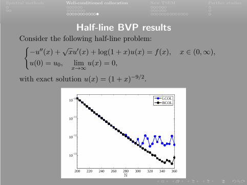
Half-line BVP resultsConsider the following half-line problem:−u′′(x) +√
xu′(x) + log(1 + x)u(x) = f(x), x ∈ (0,∞),
u(0) = u0, limx→∞
u(x) = 0,
with exact solution u(x) = (1 + x)−9/2.
200 220 240 260 280 300 320 340 360
10−13
10−12
10−11
10−10
N
LCOLBCOL
Spectral methods Well-conditioned collocation New TSEM Further studies
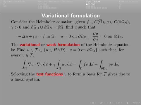
Variational formulationConsider the Helmholtz equation: given f ∈ C(Ω), g ∈ C(∂ΩN),γ > 0 and ∂ΩD ∪ ∂ΩN = ∂Ω, find u such that
−∆u+γu = f in Ω; u = 0 on ∂ΩD;∂u
∂~n= 0 on ∂ΩN.
The variational or weak formulation of the Helmholtz equationis: Find u ∈ T ⊂ u ∈ H1(Ω) , u = 0 on ∂ΩD such that, forevery v ∈ T ,
∫
Ω∇u · ∇v d~x+ γ
∫
Ωuv d~x =
∫
Ωfv d~x+
∫
∂ΩN
gv d~s.
Selecting the test functions v to form a basis for T gives rise toa linear system.

Spectral methods Well-conditioned collocation New TSEM Further studies
Variational formulationConsider the Helmholtz equation: given f ∈ C(Ω), g ∈ C(∂ΩN),γ > 0 and ∂ΩD ∪ ∂ΩN = ∂Ω, find u such that
−∆u+γu = f in Ω; u = 0 on ∂ΩD;∂u
∂~n= 0 on ∂ΩN.
The variational or weak formulation of the Helmholtz equationis: Find u ∈ T ⊂ u ∈ H1(Ω) , u = 0 on ∂ΩD such that, forevery v ∈ T ,
B (∇u,∇v) = (∇u,∇v)Ω+γ (u, v)Ω = (f, v)Ω+〈g, v〉∂ΩN= G(v).
Selecting the test functions v to form a basis for T gives rise toa linear system.
Often, for spectral methods, Ω = (−1, 1)d, and T ⊂ PdN , the
space of tensorial polynomials of degree N in each component.Data gives interpolations IIN f ∈ Pd
N and IN g ∈ Pd−1N .
Spectral methods Well-conditioned collocation New TSEM Further studies
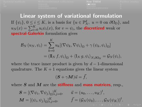
Linear system of variational formulationIf ψi, 0 ≤ i ≤ K, is a basis for u ∈ Pd
N , u = 0 on ∂ΩD, anduN (x) =
∑Ki=0 uiψi(x), for v = ψi, the discretized weak or
spectral-Galerkin formulation gives
BN (uN , ψi) =K∑
k=0
uk[(∇ψk,∇ψi)Ω + γ (ψk, ψi)Ω]
= (IIN f, ψi)Ω + 〈IN g, ψi〉N,∂ΩN= GN (ψi),
where the trace inner product is given by d− 1-dimensionalquadrature. The K + 1 equations gives the linear system
(S + γM)~u = ~f,
where S and M are the stiffness and mass matrices, resp.,
S = [(∇ψi,∇ψj)Ω]Ki,j=0, ~u = (u0, . . . , uK)t,
M = [(ψi, ψj)Ω]Ki,j=0,
~f = (GN (ψ0), . . . ,GN (ψK))t.
Spectral methods Well-conditioned collocation New TSEM Further studies
Spectral element method
Spectral element methods solve differential equations oversubdomains piecewise, in conjunction with some domain
decomposition method.

Spectral methods Well-conditioned collocation New TSEM Further studies
Spectral element method
Spectral element methods solve differential equations oversubdomains piecewise, in conjunction with some domaindecomposition method.
As in the finite-element method, let the domain Ω be asimplex.
Consider first the reference triangle
= (x, y), 0 < x, y, x+ y < 1
on the xy-plane. Herein, consider maps from the reference
square = (−1, 1)2 on the ξη-plane to , with the plan oftransforming the domain to to perform the operations.
Spectral methods Well-conditioned collocation New TSEM Further studies
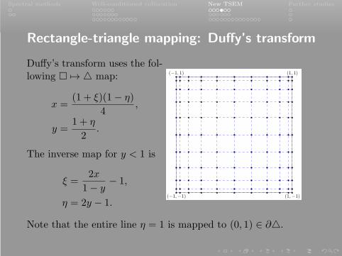
Rectangle-triangle mapping: Duffy’s transform
Duffy’s transform uses the fol-lowing 7→ map:
x =(1 + ξ)(1− η)
4,
y =1 + η
2.
The inverse map for y < 1 is
ξ =2x
1− y− 1,
η = 2y − 1.(−1,−1) (1,−1)
(1, 1)(−1, 1)
Note that the entire line η = 1 is mapped to (0, 1) ∈ ∂.

Spectral methods Well-conditioned collocation New TSEM Further studies
Rectangle-triangle mapping: Duffy’s transform
Duffy’s transform uses the fol-lowing 7→ map:
x =(1 + ξ)(1− η)
4,
y =1 + η
2.
The inverse map for y < 1 is
ξ =2x
1− y− 1,
η = 2y − 1.(0, 0) (1, 0)
(0, 1)
Note that the entire line η = 1 is mapped to (0, 1) ∈ ∂.
Spectral methods Well-conditioned collocation New TSEM Further studies
Transformed gradient for Duffy’s transform
Using the → map, given u(x, y) ∈ H1(), determineu(ξ, η) = u(x, y).
For Duffy’s transform, the Jacobian is
J =1− η
8,
and the gradient on is transformed on to
∇u =2
1− η
(2∂ξu, (1 + ξ)∂ξu+ (1− η)∂ηu
),
which requires the consistency condition ∂ξu(ξ, 1) = 0 to bebuilt into the approximation space to obtain high-orderaccuracy, resulting in the reduction of dimension andmodification of the usual basis functions.
Spectral methods Well-conditioned collocation New TSEM Further studies
New triangular spectral-element methodDuffy’s transform generates clustering near one vertex and asingularity in the gradient that requires modifying basiselements, and interpolations cannot be generated by acorresponding nodal basis on , as one edge on ∂ is mappedto a vertex on ∂.
A new transform is used that introduces less clustering, andintroduces a singularity in the gradient that is analyticallyremovable in the inner product of the variational form, whichis also one-to-one, allowing for good interpolations generatedby a corresponding nodal basis on . The function space shouldallow for optimal projection error.
Removing the singularity has to be done carefully. In addition,the singularity induced by the transform is a hanging node
when used in combination with domain decomposition methods.
Spectral methods Well-conditioned collocation New TSEM Further studies
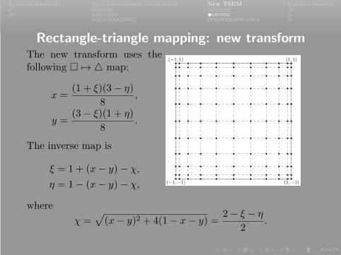
Rectangle-triangle mapping: new transformThe new transform uses thefollowing 7→ map:
x =(1 + ξ)(3− η)
8,
y =(3− ξ)(1 + η)
8.
The inverse map is
ξ = 1 + (x− y)− χ,
η = 1− (x− y)− χ, (−1,−1) (1,−1)
(1, 1)(−1, 1)
where
χ =√(x− y)2 + 4(1− x− y) =
2− ξ − η
2.

Spectral methods Well-conditioned collocation New TSEM Further studies
Rectangle-triangle mapping: new transformThe new transform uses thefollowing 7→ map:
x =(1 + ξ)(3− η)
8,
y =(3− ξ)(1 + η)
8.
The inverse map is
ξ = 1 + (x− y)− χ,
η = 1− (x− y)− χ, (0, 0) (1, 0)
(0, 1)
( 1
2,
1
2)
where
χ =√(x− y)2 + 4(1− x− y) =
2− ξ − η
2.
Spectral methods Well-conditioned collocation New TSEM Further studies
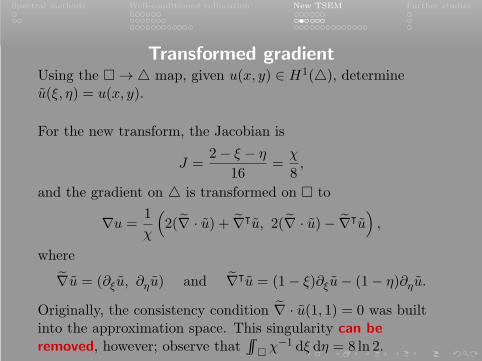
Transformed gradientUsing the → map, given u(x, y) ∈ H1(), determineu(ξ, η) = u(x, y).
For the new transform, the Jacobian is
J =2− ξ − η
16=χ
8,
and the gradient on is transformed on to
∇u =1
χ
(2(∇ · u) + ∇⊺u, 2(∇ · u)− ∇⊺u
),
where
∇u = (∂ξu, ∂ηu) and ∇⊺u = (1− ξ)∂ξu− (1− η)∂ηu.
Originally, the consistency condition ∇ · u(1, 1) = 0 was builtinto the approximation space. This singularity can be
removed, however; observe that∫∫
χ−1 dξ dη = 8 ln 2.

Spectral methods Well-conditioned collocation New TSEM Further studies
Function space
Using the → map of the new transform, givenu(ξ, η) ∈ P2
N = QN (), determine u(x, y) = u(ξ, η). Then
u(x, y) = p(x, y) + χ(x, y)q(x, y)
∈ YN () = PN ()⊕ χPN−1(),
where p ∈ PN () has total degree N , and q ∈ PN−1().
This transformation is bijective: u ∈ YN () is mapped tou ∈ QN (), using the → inverse map of the newtransform.

Spectral methods Well-conditioned collocation New TSEM Further studies
Nodal and modal basisLet ζj, 0 ≤ j ≤ N , be the Legendre-Gauss-Lobatto points,and let Lj be the Lagrange interpolation basis on ζj. Thenodal basis of YN () on nodes
(xij , yij) =
((1 + ζi)(3− ζj)
8,(3− ζi)(1 + ζj)
8
)
is Ψij, 0 ≤ i, j ≤ N , where
Ψij(x, y) = Li(1 + (x− y)− χ)Lj(1− (x− y)− χ).
Consider the C0-modal basis on (−1, 1):
φ0(ζ) =1− ζ
2, φN (ζ) =
1 + ζ
2, φi(ζ) =
i(Pi−1(ζ)− Pi+1(ζ))
2(2i+ 1),
where 0 < i < N and Pi are the Legendre polynomials. Themodal basis of YN () is Ψij, 0 ≤ i, j ≤ N , where
Ψij(x, y) = φi(1 + (x− y)− χ)φj(1− (x− y)− χ).

Spectral methods Well-conditioned collocation New TSEM Further studies
Projection error
Consider the projection ΠN : L2() → YN (),
(ΠNu− u, v) = 0, for all v ∈ YN ().
Theorem
For any u ∈ Hr(), with r ≥ 0,
‖ΠNu− u‖ ≤ cN−r|u|r,,
where c is a positive constant independent of N and u.

Spectral methods Well-conditioned collocation New TSEM Further studies
Projection error
Consider the projection Π1N : H1() → YN (),
(∇(Π1
Nu− u),∇v) +
(Π1
Nu− u, v) = 0, for all v ∈ YN ().
Theorem
For any u ∈ Hr(), with r ≥ 1,
‖Π1Nu− u‖µ, ≤ cNµ−r|u|r,, µ = 0, 1,
where c is a positive constant independent of N and u.

Spectral methods Well-conditioned collocation New TSEM Further studies
Projection error
Consider the projectionΠ1,0
N : H10 () → Y 0
N () = YN () ∩H10 (),
(∇(Π1,0
N u− u),∇v)
= 0, for all v ∈ Y 0N ().
Theorem
For any u ∈ H10 () ∩Hr(), with r ≥ 1,
‖Π1,0N u− u‖µ, ≤ cNµ−r|u|r,, µ = 0, 1,
where c is a positive constant independent of N and u.

Spectral methods Well-conditioned collocation New TSEM Further studies
Interpolation error
Let ζj, 0 ≤ j ≤ N , be the Legendre-Gauss-Lobatto points,
and Ψij be the nodal basis of YN (). Given any u ∈ C(),define the interpolant of u by
(IIN u)(x, y) =N∑
i,j=0
u
((1 + ζi)(3− ζj)
8,(3− ζi)(1 + ζj)
8
)Ψij(x, y)
∈ YN ().
Theorem
For any u ∈ Hr(), with r ≥ 3,
‖IIN u− u‖µ, ≤ cN−r(|u|r, + |u|r−1,),
where c is a positive constant independent of N and u.

Spectral methods Well-conditioned collocation New TSEM Further studies
Interpolation error
Let ζj, 0 ≤ j ≤ N , be the Legendre-Gauss-Lobatto points,
and Ψij be the nodal basis of YN (). Given any u ∈ C(),define the interpolant of u by
(IIN u)(x, y) =N∑
i,j=0
u
((1 + ζi)(3− ζj)
8,(3− ζi)(1 + ζj)
8
)Ψij(x, y)
∈ YN ().
Theorem
For any u ∈ H2(),
‖IIN u−u‖µ, ≤ cN−2(|u|2,+‖(∂y−∂x)2u‖χ−1,+‖∇·u‖χ−1,),
where c is a positive constant independent of N and u.

Spectral methods Well-conditioned collocation New TSEM Further studies
Computing the mass matrix
Let ψij, 0 ≤ i, j ≤ N , be a basis of YN (), and
φij(ξ, η) =N∑
m,n=0
pmnij Pm(ξ)Pn(η) = ψij(x, y).
Then M = P′MP , where P = [pmn
ij ], 0 ≤ i, j,m, n ≤ N and
M is a pentadiagonal matrix whose entries are
1
16
∫∫
Pm(ξ)Pm′(ξ)Pn(η)Pn′(η)(2− ξ − η) dξ dη,
where 0 ≤ m,n,m′, n′ ≤ N .

Spectral methods Well-conditioned collocation New TSEM Further studies
Computing the stiffness matrix
Let ψij, 0 ≤ i, j ≤ N , be a basis of YN (), andφij(ξ, η) = ψij(x, y). Then S = S1 + S2, where
S1 =
[(∇ · φij , ∇ · φi′j′
)χ−1,
]N
i,j,i′,j′=0
,
S2 =1
4
[(∇⊺φij , ∇⊺φi′j′
)χ−1,
]N
i,j,i′,j′=0
.
Each entry is a computable combination of
apq =
∫∫
Pp(ξ)Pq(η)
χdξ dη, 0 ≤ p, q ≤ 2N.

Spectral methods Well-conditioned collocation New TSEM Further studies
Computing the stiffness matrix
Let ψij, 0 ≤ i, j ≤ N , be a basis of YN (), andφij(ξ, η) = ψij(x, y). Then S = S1 + S2, where
S1 =
∫∫
(∇ · φij)(∇ · φi′j′)χ
dξ dη
N
i,j,i′,j′=0
,
S2 =1
4
∫∫
(∇⊺φij)(∇⊺φi′j′)
χdξ dη
N
i,j,i′,j′=0
.
Each entry is a computable combination of
apq =
∫∫
Pp(ξ)Pq(η)
χdξ dη, 0 ≤ p, q ≤ 2N.

Spectral methods Well-conditioned collocation New TSEM Further studies
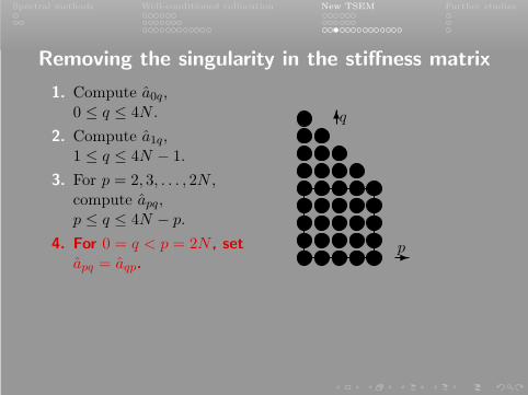
Removing the singularity in the stiffness matrix
1. Compute a0q,0 ≤ q ≤ 4N . q
p
Use
a0q =
∫ 1
−1Pq(η) ln
3− η
2︸ ︷︷ ︸by quadrature
+
∫ 1
−1Pq(η) ln
2
1− η︸ ︷︷ ︸2 if q=0, else 2/q(q+1)
.
Spectral methods Well-conditioned collocation New TSEM Further studies
Removing the singularity in the stiffness matrix
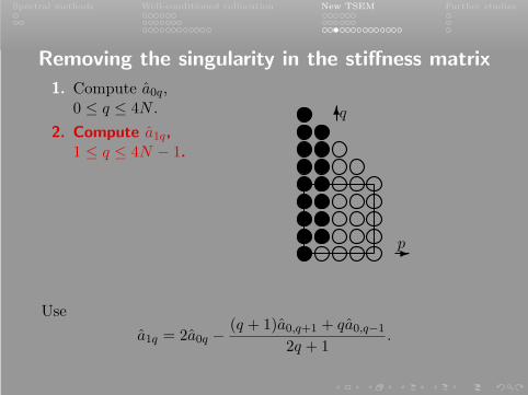
1. Compute a0q,0 ≤ q ≤ 4N .
2. Compute a1q,1 ≤ q ≤ 4N − 1.
q
p
Use
a1q = 2a0q −(q + 1)a0,q+1 + qa0,q−1
2q + 1.

Spectral methods Well-conditioned collocation New TSEM Further studies
Removing the singularity in the stiffness matrix
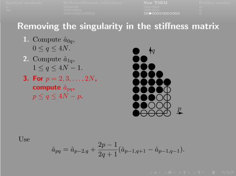
1. Compute a0q,0 ≤ q ≤ 4N .
2. Compute a1q,1 ≤ q ≤ 4N − 1.
3. For p = 2, 3, . . . , 2N ,
compute apq,p ≤ q ≤ 4N − p.
q
p
Use
apq = ap−2,q +2p− 1
2q + 1(ap−1,q+1 − ap−1,q−1).

Spectral methods Well-conditioned collocation New TSEM Further studies
Removing the singularity in the stiffness matrix
1. Compute a0q,0 ≤ q ≤ 4N .
2. Compute a1q,1 ≤ q ≤ 4N − 1.
3. For p = 2, 3, . . . , 2N ,
compute apq,p ≤ q ≤ 4N − p.
q
p
Use
apq = ap−2,q +2p− 1
2q + 1(ap−1,q+1 − ap−1,q−1).
Spectral methods Well-conditioned collocation New TSEM Further studies
Removing the singularity in the stiffness matrix
1. Compute a0q,0 ≤ q ≤ 4N .
2. Compute a1q,1 ≤ q ≤ 4N − 1.
3. For p = 2, 3, . . . , 2N ,
compute apq,p ≤ q ≤ 4N − p.
q
p
Use
apq = ap−2,q +2p− 1
2q + 1(ap−1,q+1 − ap−1,q−1).
Spectral methods Well-conditioned collocation New TSEM Further studies
Removing the singularity in the stiffness matrix
1. Compute a0q,0 ≤ q ≤ 4N .
2. Compute a1q,1 ≤ q ≤ 4N − 1.
3. For p = 2, 3, . . . , 2N ,compute apq,p ≤ q ≤ 4N − p.
4. For 0 = q < p = 2N , set
apq = aqp.
q
p
Spectral methods Well-conditioned collocation New TSEM Further studies
Numerical resultsConsider the elliptic equation:
−∆u+u = f in ; u|Γ1= 0;
∂u
∂~n
∣∣∣Γ2
= g,
where Γ1 is the edges x = 0 and y = 0, Γ2 is the hypotenuse of, and with the exact solution:
u(x, y) = ex+y−1 sin(3xy
(y −
√32 x+
√34
)).
For comparison, consider
−∆u+u = f in S = (0, 1/√2)2; u|Γ′
1= 0;
∂u
∂~n
∣∣∣Γ′
2
= g,
where Γ′1 is the edges x = 0 and y = 0 and Γ′
2 is the edgesx = 1/
√2 and y = 1/
√2, with exact solution
u(x, y) = exp(−(
1√2− x)(
1√2− y))
sin(3xy
(y −
√32 x+
√34
)).
Spectral methods Well-conditioned collocation New TSEM Further studies
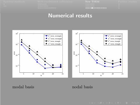
Numerical results
5 10 15 20 25
10−15
10−10
10−5
100
N
erro
r
L2 error, rectangle
L∞ error, rectangle
L2 error, triangle
L∞ error, triangle
modal basis
5 10 15 20 25
10−15
10−10
10−5
100
Ner
ror
L2 error, rectangle
L∞ error, rectangle
L2 error, triangle
L∞ error, triangle
nodal basis

Spectral methods Well-conditioned collocation New TSEM Further studies
Numerical results
Consider the elliptic equation:
−∆u+u = f in ; u|Γ1= 0;
∂u
∂~n
∣∣∣Γ2
= g,
where Γ1 is the edges x = 0 and y = 0, Γ2 is the hypotenuse of, with the finite regularity exact solution:
u(x, y) = (1− x− y)52 (exy − 1) ∈ H3−ǫ()
The counterpart on the square S takes the form:
u(x, y) =
(1√2− x
) 52(
1√2− y
) 52
(exy − 1), ∀ (x, y) ∈ S.

Spectral methods Well-conditioned collocation New TSEM Further studies
Numerical results
0.6 0.8 1 1.2 1.4 1.6−8
−7
−6
−5
−4
−3
−2
log10
(N)
log 10
(err
or)
L2 error, rectangle
L∞ error, rectangle
L2 error, triangle
L∞ error, triangle
modal basis
0.6 0.8 1 1.2 1.4 1.6−8
−7
−6
−5
−4
−3
−2
log10
(N)lo
g 10(e
rror
)
L2 error, rectangle
L∞ error, rectangle
L2 error, triangle
L∞ error, triangle
nodal basis

Spectral methods Well-conditioned collocation New TSEM Further studies
Arbitrary triangleFor a triangle any, with vertices counterclockwise at (x1, y1),(x2, y2) and (x3, y3), the invertible map → any is
(x, y) = (x1, y1)(1− ξ)(1− η)
4+ (x2, y2)
(1 + ξ)(3− η)
8
+ (x3, y3)(3− ξ)(1 + η)
8.
Using this map to determine u(ξ, η) = u(x, y), the mass matrixis determined by
(u, v)any=F
8(u, v)χ, ,
where
F = (x2 − x1)(y3 − y1)− (x3 − x1)(y2 − y1) 6= 0.

Spectral methods Well-conditioned collocation New TSEM Further studies
Arbitrary triangle
For a triangle any, with vertices counterclockwise at (x1, y1),(x2, y2) and (x3, y3), the invertible map → any is
(x, y) = (x1, y1)(1− ξ)(1− η)
4+ (x2, y2)
(1 + ξ)(3− η)
8
+ (x3, y3)(3− ξ)(1 + η)
8.
Using this map to determine u(ξ, η) = u(x, y), the stiffnessmatrix is determined by
(∇u,∇v)any=
A
2F
(∇ · u, ∇ · v
)χ−1,
+C
8F
(∇⊺u, ∇⊺v
)χ−1,
− B
4F
[(∇ · u, ∇⊺v
)χ−1,
+(∇⊺u, ∇ · v
)χ−1,
].
where A, B and C are determined from xi, yi, 1 ≤ i ≤ 3.

Spectral methods Well-conditioned collocation New TSEM Further studies
Unstructured TSEM with LDG-H
To use this TSEM on an unstructured mesh, the hybridized
local discontinuous Galerkin method is used.
• DG methods enjoy a large degree of flexibility,non-conformity and locality. In particular, DG methods
can handle hanging nodes in meshes, while providing ascheme to handle the coupling on the mesh. Having thehanging node in a predictable position allows for efficientcomputation.
• LDG-H makes use of auxillary functions, which renders theelliptic problem into a system of first-order differentialequations. For those inner products, the rectangle-triangle
map does not induce a singularity.
• LDG-H generates a global system whose degrees of
freedom are only those on the interior edges.

Spectral methods Well-conditioned collocation New TSEM Further studies
Results for unstructured TSEMConsider the model problem
−∆u+u = f, in Ω = [0, 1]2; u = 0 on ∂Ω,
with the highly-oscillating exact solution
u(x, y) = sin(10πx) cos(10πy).
0 0.2 0.4 0.6 0.8 10
0.2
0.4
0.6
0.8
1
x
y
5× 5
0 0.2 0.4 0.6 0.8 10
0.2
0.4
0.6
0.8
1
x
y
15× 15
0 0.2 0.4 0.6 0.8 10
0.2
0.4
0.6
0.8
1
xy
25× 25

Spectral methods Well-conditioned collocation New TSEM Further studies
Results for unstructured TSEM
2 4 6 8 10 12 1410
−12
10−10
10−8
10−6
10−4
10−2
100
102
Polynomial order
Ave
rage
ele
men
t−w
ise
H1 err
or
5 × 5, τ = 15 × 5, τ = 100015 × 15, τ = 115 × 15, τ = 100025 × 25, τ = 125 × 25, τ = 1000
10−1
10−8
10−6
10−4
10−2
h
Ave
rage
ele
men
t−w
ise
L2 e
rror
P = 3P = 4P = 5

Spectral methods Well-conditioned collocation New TSEM Further studies
Results for structured TSEM versus perturbationConsider the model problem
−∆u+u = f, in Ω = [0, 1]2; u = 0 on ∂Ω,
with the highly-oscillating exact solutionu(x, y) = sin(10πx) cos(10πy). Ω is triangulated into twomeshes of varying coarseness, denoted 5× 5 and 10× 10, eithermaintaining the regular underlying mesh or perturbing slightly
on the internal vertices.
5 10 15 20 25
10−12
10−14
10−10
10−8
10−6
10−4
10−2
100
N
aver
age
elem
ent−
wis
e L
2 err
or
5 10 15 20 25
10−9
10−11
10−7
10−5
10−3
10−1
101
N
aver
age
elem
ent−
wis
e H
1 err
or
Spectral methods Well-conditioned collocation New TSEM Further studies
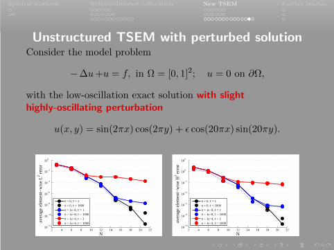
Unstructured TSEM with perturbed solutionConsider the model problem
−∆u+u = f, in Ω = [0, 1]2; u = 0 on ∂Ω,
with the low-oscillation exact solution with slight
highly-oscillating perturbation
u(x, y) = sin(2πx) cos(2πy) + ǫ cos(20πx) sin(20πy).
2 4 6 8 10 12 14 16 18 20 2210
−12
10−10
10−8
10−6
10−4
10−2
100
N
aver
age
elem
ent−
wis
e L
2 err
or
ε = 0, τ = 1ε = 0, τ = 1000ε = 1e−8, τ = 1ε = 1e−8, τ = 1000ε = 1e−4, τ = 1ε = 1e−4, τ = 1000
2 4 6 8 10 12 14 16 18 20 2210
−10
10−8
10−6
10−4
10−2
100
102
N
aver
age
elem
ent−
wis
e H
1 err
or
ε = 0, τ = 1ε = 0, τ = 1000ε = 1e−8, τ = 1ε = 1e−8, τ = 1000ε = 1e−4, τ = 1ε = 1e−4, τ = 1000

Spectral methods Well-conditioned collocation New TSEM Further studies
Unstructured TSEM with perturbed traceConsider the model problem
−∆u+u = f, in Ω = [0, 1]2; u = 0 on ∂Ω,
with the low-oscillation exact solution
u(x, y) = sin(2πx) cos(2πy).
The perturbation ǫ cos(20πx) sin(20πy) is introduced after
solving the global system, before applying the local solvers.
2 4 6 8 10 12 14 16 18 20 2210
−12
10−10
10−8
10−6
10−4
10−2
100
N
aver
age
elem
ent−
wis
e L
2 err
or
ε = 0, τ = 1
ε = 0, τ = 1000
ε = 1e−8, τ = 1
ε = 1e−8, τ = 1000
ε = 1e−4, τ = 1
ε = 1e−4, τ = 1000
2 4 6 8 10 12 14 16 18 20 2210
−10
10−8
10−6
10−4
10−2
100
102
N
aver
age
elem
ent−
wis
e H
1 err
or
ε = 0, τ = 1
ε = 0, τ = 1000
ε = 1e−8, τ = 1
ε = 1e−8, τ = 1000
ε = 1e−4, τ = 1
ε = 1e−4, τ = 1000

Spectral methods Well-conditioned collocation New TSEM Further studies
Well-conditioned collocation
Research for the method in the first part, which produceswell-conditioned collocation schemes, three directions areworthy of further investigation.
• Investigate the notion for well-conditionedpolynomial-based collocation methods for other situations,e.g., the spline collocation, radial basis functions and somenon-polynomial bases.
• Extension of the well-conditioned collocation approach tomultiple dimensions.
• Obtain the optimal error estimates for the Birkhoffinterpolations.

Spectral methods Well-conditioned collocation New TSEM Further studies
Tetrahedral spectral elements
The new TSEM on unstructured meshes based on the DGformulation is worthy of deep investigation. Furtherdevelopment can be taken in the following directions:
• Apply the TSEM to more challenging problems such as theStokes equations and the Navier-Stokes equations.
• Develop a three-dimensional unstructured tetrahedralTSEM.
• Prove global convergence of the unstructured TSEM.

Spectral methods Well-conditioned collocation New TSEM Further studies
Further reading
Robert Kirby, Spencer Sherwin and Bernardo Cockburn. ToCG or to HDG: a comparative study. Journal of ScientificComputing, vol. 51 (1), 183–212, 2012
Michael Daniel Samson, Li-Lian Wang and Huiyuan Li. Anew triangular spectral element method I:
implementation and analysis on a triangle. NumericalAlgorithms, vol. 64 (3), 519–547, 2013
Li-Lian Wang, Michael Daniel Samson and Xiaodan Zhao.A well-conditioned collocation method using a
pseudospectral integration matrix. Accepted to SIAMJournal on Scientific Computing, 2014