WELL CONTROL MODEL

THEORY AND USER'S MANUAL

DEA 67 PHASE l

MAURER ENGINEERING INC. 2916 West T.C. Jester Houston, Texas 7701 8

WELL CONTROL MODEL

(WELCON2)

Theory and User's Manual

MAURER ENGINEERING INC. 2916 West T.C. Jester Boulevard

Houston, TX 77018-7098

Telephone: 7131683-8227 Telex: 216556 Facsimile: 7131683-6418

February, 1993

TR93-2

This copyrighted 1993 confidential report and the computer programs are for the sole use of Participants on the Drilling Engineering Association DEA-44 project to DEVELOP AND EVALUATE HORIZONTAL DRILLING TECHNOLOGY andlor DEA-67 project to DEVELOP AND EVALUATE SLIM-HOLE AND COILED-TUBING TECHNOLOGY and their afiliates, and are not to be disclosed to other parties. Data output ¶ram the programs can be disclosed to third parties. Participants and their affiliates are free to make copies of this report and programs for their own use.

Table of Contents

Page

1 . INTRODUCTION . . . . . . . . . . . . . . . . . . . . . . . . . . . . . . . . . . . . . . . . . . . . . 1-1

1.1 MODEL FEATURES OF WELCON2 . . . . . . . . . . . . . . . . . . . . . . . . . . . 1-1

1.2 WHAT IS NEW IN WELCON2 . . . . . . . . . . . . . . . . . . . . . . . . . . . . . . . 1-2

1.3 REQUIRED INPUT DATA . . . . . . . . . . . . . . . . . . . . . . . . . . . . . . . . . . 1-2

1.4 DISCLAIMER . . . . . . . . . . . . . . . . . . . . . . . . . . . . . . . . . . . . . . . . . . 1-3

1.5 COPYRIGHT . . . . . . . . . . . . . . . . . . . . . . . . . . . . . . . . . . . . . . . . . . . 1-3

2 . THEORY AND EQUATIONS . . . . . . . . . . . . . . . . . . . . . . . . . . . . . . . . . . . . . 2-1

2.1 APPROACH . . . . . . . . . . . . . . . . . . . . . . . . . . . . . . . . . . . . . . . . . . . 2-1

2.2 RESERVOIR MODEL (Nickens. 1987) . . . . . . . . . . . . . . . . . . . . . . . . . . 2-2

2.3 DRILL-PIPE MODEL . . . . . . . . . . . . . . . . . . . . . . . . . . . . . . . . . . . . . 2-3

2.4 ANNULUS MODEL . . . . . . . . . . . . . . . . . . . . . . . . . . . . . . . . . . . . . . 2-4

2.5 SINGLE-BUBBLE MODEL (LeBlanc and Lewis. 1967) . . . . . . . . . . . . . . . 2-6

2.6 TWO-PHASE FLOW MODEL . . . . . . . . . . . . . . . . . . . . . . . . . . . . . . . 2-6

2.7 GAS SOLUBILITY CORRELATION (O'Brian et al.. 1988) . . . . . . . . . . . . . 2-9

2.8 SOLUTION ALGORITHM (Santos. 1991) . . . . . . . . . . . . . . . . . . . . . . . . 2-10

2.8.1 Finite Difference Equations . . . . . . . . . . . . . . . . . . . . . . . . . . . . . 2-11 2.8.2 Boundary Conditions . . . . . . . . . . . . . . . . . . . . . . . . . . . . . . . . . 2-12

. . . . . . . . . . . . . . . . . . . . . . . . . . . . . . . . 2.8.3 Initial Conditions 2-12 2.8.4 Solution Procedure . . . . . . . . . . . . . . . . . . . . . . . . . . . . . . . . . . 2-12

2.9 RHEOLOGY MODEL . . . . . . . . . . . . . . . . . . . . . . . . . . . . . . . . . . . . . 2-14

2.9.1 Bingham Plastic Model . . . . . . . . . . . . . . . . . . . . . . . . . . . . . . . . 2-14 2.9.2 Power-Law Model . . . . . . . . . . . . . . . . . . . . . . . . . . . . . . . . . . . 2-17

2.10 EQUIVALENT CIRCULATING DENSITY . . . . . . . . . . . . . . . . . . . . . . . 2-20

2.11 TWO-PHASE FLOW CORRELATIONS . . . . . . . . . . . . . . . . . . . . . . . . . 2-20

2.11.1 Beggs-Brill Correlation (Beggs and Brill. 1973) . . . . . . . . . . . . . . . . 2-21 2.11.2 Hagedorn-Brown Correlation (Brown and Beggs. 1977) . . . . . . . . . . . 2-24 2.11.3 Hasan-Kabir Correlation (Hasan and Kabir. 1992) . . . . . . . . . . . . . . 2-26

3 . PROGRAM INSTALLATION . . . . . . . . . . . . . . . . . . . . . . . . . . . . . . . . . . . . . 3-1

3.1 BEFORE INSTALLING . . . . . . . . . . . . . . . . . . . . . . . . . . . . . . . . . . . . 3-1

3.1.1 Hardware and System Requirements . . . . . . . . . . . . . . . . . . . . . . . 3-1 3.1.2 Check the Program Disk . . . . . . . . . . . . . . . . . . . . . . . . . . . . . . . 3-2 3.1.3 Backup Disk . . . . . . . . . . . . . . . . . . . . . . . . . . . . . . . . . . . . . . . 3-3

3.2 INSTALLING WELCON2 . . . . . . . . . . . . . . . . . . . . . . . . . . . . . . . . . . 3-3

3.3 STARTING WELCON2 . . . . . . . . . . . . . . . . . . . . . . . . . . . . . . . . . . . . 3-4

Table of Contents (Cont ' d.)

Page

3.3.1 Start WELCON2 from Group Window . . . . . . . . . . . . . . . . . . . . . 3-4 3.3.2 Use Command-Line Option from Windows . . . . . . . . . . . . . . . . . . . 3-4

3.4 ALTERNATIVE SETUP . . . . . . . . . . . . . . . . . . . . . . . . . . . . . . . . . . . 3-5

. . . . . . . . . . . . . . . . . . . . . . . . . . . . . . . . . . 4 . QUICK START WITH EXAMPLE 4-1

4.1 INTRODUCTORY REMARKS . . . . . . . . . . . . . . . . . . . . . . . . . . . . . . . 4-1

4.2 GETTINGSTARTED . . . . . . . . . . . . . . . . . . . . . . . . . . . . . . . . . . . . . 4-1

5 . OPTIONS AND CHOICES OF THE MODEL . . . . . . . . . . . . . . . . . . . . . . . . . . . 5-1

5.1 INPUTDATA . . . . . . . . . . . . . . . . . . . . . . . . . . . . . . . . . . . . . . . . . . 5-1

5.2 SDI AND TDI DATA INPUTS . . . . . . . . . . . . . . . . . . . . . . . . . . . . . . . 5-2

5.3 PARAMETER DATA INPUT . . . . . . . . . . . . . . . . . . . . . . . . . . . . . . . . 5-2

6 . REFERENCES . . . . . . . . . . . . . . . . . . . . . . . . . . . . . . . . . . . . . . . . . . . . . . . 6-1

1. Introduction

Well control is one of the most important aspects of drilling operations. Improper handling of

kicks can result in blowouts with potential loss of life and equipment. To help prevent such disasters,

Maurer Engineering Inc. has developed a well control windows application, WELCON2, as part of the

DEA-44 Project to "Develop and Evaluate Horizontal Well Technology" and the DEA-67 Project to

"Develop and Evaluate Slim-Hole and Coiled-Tubing Technology." This program is written in Visual

Basic 1.0 for use with IBM compatible computers. Program WELCON2 runs in Windows 3.0 or later

versions. WELCON2 will run with 80286 or higher processors (with math co-processors), but run

times may be long with 80286 processors due to the large number of calculations (see Table 3-1).

The program describes the complex multiphase flow as a gas influx is circulated out of the well.

The mathematical model consists of differential equations that are solved using finite difference methods.

The model is suitable for 3D wellbores (vertical and horizontal) for inland and offshore applications.

It handles both Driller's and Engineer's methods and uses Bingham plastic and power-law fluid models

- for frictional pressure calculations. The program allows the user to select either a single-bubble model

(water-based mud only) or one of three two-phase flow correlations for handling gas migration in the

wellbore. It takes into account the effect of gas solubility when oil-based mud is used. - h

The program calculates kill-mud weight and drill-pipe pressure schedule. It predicts pressure

- changes and equivalent circulating densities (ECD) at the choke, casing shoe, wellhead, at the end of the

well, and at any other one point the user specifies (e.g., entrance to horizontal section). The maximum

ECD along the wellbore is also calculated and compared with the pore pressure gradient and fracture

pressure gradient. These results are useful for determining equipment adequacy and kick tolerance.

Every effort has been made to ensure that WELCON2 will converge to a meaningful solution

over the expected range of input variables. However, it is conceivable that the mathematical system may

exhibit instability for one or more combinations of input variables. Should this occur, we would

appreciate being advised of the circumstances leading to the failure of WELCON2 and the nature of the

output generated.

1.1 MODEL FEATURES OF WELCON2

The key features of WELCON2 are its ability to:

1. Handle both water-based and oil-based muds.

2. Deal with 3D wellbores.

3. Select either single-bubble or one of three flow correlations.

4. Handle inland and offshore drilling rigs.

5. Handle both Driller's and Engineer's method.

6. Handle fifteen (15) sections of drill string and ten (10) well intervals.

7. Use Bingham Plastic or Power-Law models.

8. Use two-unit system: English and metric.

The output window is a compilation of chid windows of text reports and graphs, which include:

1. Summary report.

2. Tabulated results.

3. Pressure or ECD at choke, drill pipe, bottom hole, casing shoe, wellhead, and user-specified point.

4. Pit gain and gas flow rate.

5. Maximum ECD along wellbore compared with pore pressure gradient and fracture pressure gradient.

1.2 WHAT IS NEW IN WELCONZ

1. Oil-based mud is added to the model. The effect of gas solubility in the oil-based mud is taken into account.

2. In WELCON1, user is required to input the gas distribution along the wellbore. In WELCONZ, a gas kick-in model is used to calculate the distribution.

3. WELCONZ allows user either to include gas kick-in period in the report or exclude it by selecting time origin.

4. The TEXT REPORT is taken out. It is consolidated into the SUMMARY REPORT in WELCONZ.

5. Different curves of the same kind can be plotted on one page for easy comparison. User decides what to plot.

6. User can print or plot pit gain and gas flow rate as a function of time.

1.3 REQUIRED INPUT DATA

There are four data files associated with WELCONZ:

1. Survey data file (.SDI).

a. Directional survey data for the well. Survey must start with zero depth, zero azimuth, and zero inclination.

2. Tubular data file (.WTl).

a. Bit depth.

b. Casing set depth.

c. Pump data.

d. Drilling bit data.

e. Lengths, ID and OD of drill string.

f. Positions and IDS of choke line, casing and open hole.

3. Parameter data file (.WPl).

a. Shut-in data.

b. Gas influx data.

c. Original drilling mud data.

d. Kill-mud data.

e. Temperature distribution along wellbore.

f. Pore pressure gradient and fracture pressure gradient.

4. Project data file with the extension name (.PJT).

The project file only stores names of three files mentioned above.

All input data saved on the disk or in memory are in the English system of units.

- 1.4 DISCLAIMER

No warranty or representation is expressed or implied with respect to these programs or

- F documentation including their quality, performance, merchantability, or fitness for a particular purpose.

1.5 COPYRIGHT

Participants in DEA-44/67 can provide data output from this copyrighted program to their

affiliates and can duplicate the program and manual for their in-house use, but this data is not to be

disclosed to other parties.

2. Theory and Equations

2.1 APPROACH

Figure 2-1 illustrates the conceptual approach used to model the areas of interest in the well

system. The drilling fluid, referred to as the liquid phase, is pumped into the drill pipe, flows through

the bit, up the annulus, and exits through the choke. After drilling into an overpressured gas sand, the

gas Nck fluid) enters the wellbore creating a two-phase mixture region. If oil-based mud is used, some

of the gas will be dissolved in the mud. The rest of the gas remains as free gas if pressure is smaller

than the saturation pressure. The objective of the well control is to circulate the gas out of the annulus

through the choke while maintaining the bottom-hole pressure (BHP) at the formation pressure to prevent

further gas influx. The gas circulation can be initiated by pumping either original drilling mud (Driller's

method) or heavier kill mud (Engineer's method).

ORIGINAL DENSITY

FLOW

Figure 2-1. Well-Control Flow Pattern

After a gas influx (kick) has been recognized and the well is shut in, two quantities should be

determined:

1. Shut-in drill-pipe pressure, (SIDPP).

2. Influx volume @it gain).

Influx volume can be easily determined from a pit gain recording.

The formation pressure is calculated from the following equation:

Pi = SIDPP + 0.052 ' p,,, ' TVD, (psi)

The kill-mud weight is determined by:

bh P, =

0.052.TVD (PPP)

The bottom-hole pressure is maintained by adjusting the choke such that the drill pipe pressure

follows a precalculated schedule.

A two-step procedure is used to simulate the kick behavior in the annulus. The first-step uses

a kick-in model to simulate the gas kick-in process. This step ends when either pit gain reaches the

specified value or the well is producing free gas before the specified pit gain is reached. The final result

from this step is the gas distribution in the annulus which will be used in the next step: the kill model.

In reality, there is a shut-in period between the kick-in period and the kill period. However, the shut-in

period is not modeled in this program.

The kick-in model assumes that the choke is wide-open. The bottom-hole pressure is then

determined by calculating the hydrostatic and frictional pressure loss in the annulus. If the calculated

bottom-hole pressure is smaller than the formation pressure, gas kicks in. The gas influx rate is

determined from the reservoir model. The bottom-hole pressure may increase or decrease due to the gas influx.

This change in pressure will affect the influx rate. all these changes are reflected in the reservoir model.

The kill model assumes that the bottom-hole pressure is always maintained at formation pressure.

There is no additional gas influx during the kill process. When kill mud fills most of the annulus, the

bottom-hole pressure may have to be raised above the formation pressure to overcome the increased

frictional pressure loss. The kill model consists of two parts. One is for calculating the drill pipe

pressure schedule (Drill Pipe Model), another is for calculating pressure behavior in the annulus

(Annulus Model). These two models will be discussed in greater detail in sections following.

2.2 RESERVOIR MODEL (Nickens, 1987)

During the kick-in process, the drilling continues at the rate of penetration (ROP). An increasing

portion of the formation is exposed to the gas flow. To model this dynamic flow process, the formation

is divided into a series of segments of thickness hi equal to the ROP times the time step during which that

segment was first exposed to the wellbore. Each time step for which the ROP is non-zero generates a

- new h,. Each segment generated is updated after each time step so that the total time of exposure of each - segment is constantly increasing as the kick progresses. -

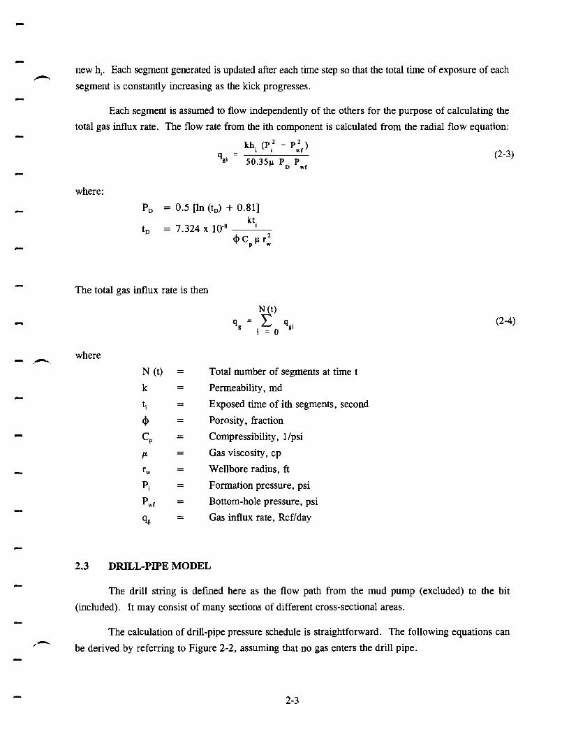
Each segment is assumed to flow independently of the others for the purpose of calculating the

total gas influx rate. The flow rate from the ith component is calculated from the radial flow equation: -

where:

- P, = 0.5 [In (t,) + 0.811

The total gas influx rate is then

where

N (t) =

k - -

ti - -

4 - -

CP - -

P - -

- rw -

Pi - -

p w f - -

e - -

Total number of segments at time t

Permeability, md

Exposed time of ith segments, second

Porosity, fraction

Compressibility, llpsi

Gas viscosity, cp

Wellbore radius, ft

Formation pressure, psi

Bottom-hole pressure, psi

Gas influx rate, Rcflday

2.3 DRnGPIPE MODEL

The drill string is defmed here as the flow path from the mud pump (excluded) to the bit

(included). It may consist of many sections of different cross-sectional areas.

The calculation of drill-pipe pressure schedule is straightforward. The following equations can

be derived by referring to Figure 2-2, assuming that no gas enters the drill pipe.

During the kick-in period, Pbh is calculated assuming the choke is wide-open. During the kill

period, P,, equals the formation pressure.

1 KILL MUD A Pf.,

1 1

ORIGINAL DENSITY MUD

A 'h.odrn

Figure 2-2. Drill-Pipe Model

The pressure loss across the bit is determined as:

The frictional pressure loss inside drill pipe and annulus is calculated using either Bingham

plastic or power-law models. These two models are documented in Section 2.9.

2.4 ANNULUS MODEL

The annulus is defined as the flow path from the bit to the surface, which consists of 1) the

annular region between the drill pipe and the casing or formation, and 2) the choke line, which is a

circular pipe. As with the drill string, the annulus may have as many sections of different cross-sectional

areas as desired. However, in the program, the number of sections is limited to ten.

During the course of gas circulation, there could be as many as four sections of fluids in

annulus as shown in Figure 2-3.

ORIGINAL

Figure 2-3. Annulus Model

the

The original drilling mud section preceding the kill mud does not mix with the gas in the two-

phase region. The interface between them is distinct and never changes except by moving ahead with

the ODM section. The two-phase mixture section includes the section with both dissolved gas and free

gas (true two-phase region) and section with dissolved gas only (single-phase actually). The interface

between ODM and the two-phase mixture section below is constantly changing since the gas may slip

relative to the average mixture velocity and dissolved gas may move ahead due to dispersion.

The pressure drop in the liquid regions is determined the same way as for drill pipe. Either the

Bingham Plastic or Power Law model is used for the frictional pressure loss calculation.

The pressure drop in the two-phase section needs special treatment. For water-based mud, two

models are used for this section: 1) one treats the section as a single-bubble and 2) the other treats it

as a two-phase bubble-flow region. For oil-based mud, only the two-phase flow model can be used.

Once the pressure drop in the two-phase flow-section (A Prp) is determined, the pressure at the

choke inlet can be calculated as:

The pressure drop in the ODM section may include both of the sections below and above the two-

phase region depending on the circulation time.

The pressure at other points of interest can be evaluated in a similar way.

2.5 SINGLEBUBBLE MODEL (LeBlanc and Lewis, 1967)

As the name implies, the gas enters the wellbore at the bottom as an immiscible slug, retains

constant composition, remains immiscible and undergoes no phase change. This single-bubble of gas

stays at the bottom of the well when circulation begins. The length of gas column is determined by the

pressure and temperature at the bottom of the column. The single-bubble model applies only to water-

based mud.

Assume the pressure and temperature at the interface between the gas column and the mud below

is Pi and Ti, respectively, then the gas volume is

from which the gas column length can be determined. Hydrostatic head or frictional pressure loss

becomes readily available. V is measured by the pit gain.

2.6 TWO-PHASE now MODEL

During both kick-in and kill period, gas and liquid flow simultaneously in the annulus. Gas may

dissolve into or evolve from the liquid phase, depending on the local pressure, temperature, and bubble-

point pressure conditions. Furthermore, free gas may move faster relative to the mixture velocity due

to gas slippage. To describe this complex, twephase flow problem, a two-phase flow model is required.

Eight variables will give a complete description of the system. These include gas and mud densities,

liquid holdup, gas and mud velocities, pressure, temperature, and gas solubility. The temperature

distribution in the annulus is assumed to be known and constant throughout the process. Then, seven

equations relating the remaining variables are required to obtain a solution.

The seven equations used to describe the one-dimensional mixture system in the annulus are based

on the work of Santos, 1991:

Liquid holdup, fraction

Time, seconds

Liquid density, ppg

Liquid density at surface conditions, ppg

Gas density, ppg Liquid velocity, Wsec Gas velocity, Wsec Spatial dimension, ft Pressure, psi

Bubble-point pressure, psi Specific gravity of gas

Temperature, "R Formation volume factor, Rcf/Scf

Eqs. 2-9 and 2-10 are the mass-balance equations for the mud and gas, respectively. Eq. 2-1 1

is the momentum-balance equation for the gaslmud mixture, and Eq. 2-12 is an empirical correlation for

predicting liquid holdup from velocities and liquid and gas properties. Eq. 2-13 is the EOS (equation

of state for gas phase).

Eq. 2-1 1 is used instead of separate momentum-balance equations for each phase because of

the unknown nature of the interactive forces between the gas and mud phases. This formulation of

separated gaslliquid flow is one form of the "drift flux" model.

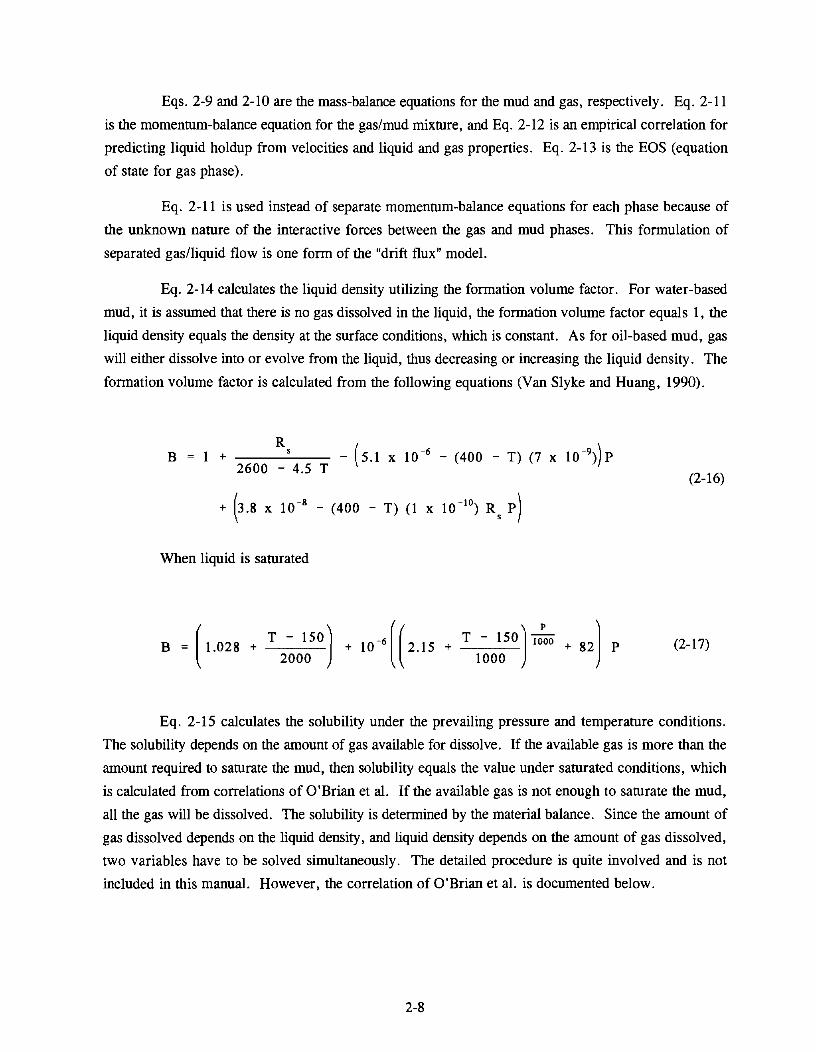
Eq. 2-14 calculates the liquid density utilizing the formation volume factor. For water-based

mud, it is assumed that there is no gas dissolved in the liquid, the formation volume factor equals 1, the

liquid density equals the density at the surface conditions, which is constant. As for oil-based mud, gas

will either dissolve into or evolve from the liquid, thus decreasing or increasing the liquid density. The

formation volume factor is calculated from the following equations (Van Slyke and Huang, 1990).

When liquid is saturated

Eq. 2-15 calculates the solubility under the prevailing pressure and temperature conditions.

The solubility depends on the amount of gas available for dissolve. If the available gas is more than the

amount required to saturate the mud, then solubility equals the value under saturated conditions, which

is calculated from correlations of O'Brian et al. If the available gas is not enough to saturate the mud,

all the gas will be dissolved. The solubility is determined by the material balance. Since the amount of

gas dissolved depends on the liquid density, and liquid density depends on the amount of gas dissolved,

two variables have to be solved simultaneously. The detailed procedure is quite involved and is not

included in this manual. However, the correlation of O'Brian et al. is documented below.

2.7 GAS SOLUBILITY CORRELATION (OfBrian et al., 1988) P.

O'Brian et al. performed an experiment to determine gas solubility in the drilling fluid under

different pressure and temperatures. The drilling fluid is composed of three components: oil, brine, and

emulsifiers. Gas is composed of two components: hydrocarbon and CO,

First, the solubility of individual component gas in individual component drilling fluid is

estimated. The gas mixture solubility in drilling fluid mixture is calculated as being the volume weighted

sum of individual solubilities.

1. The general equation for the solubility of gas in oil and emulsifiers:

Where a, b and n are shown in the following table.

TABLE 21. Correlation of Constants

2. Solubility of hydrocarbon gas in brine.

R,, = (A + BT + CTZ) B, A = 5.5601 + 8.49 x p - 3.06 x 10.' pZ

B = -0.03484 - 4.0 x 10.' P

C = 6.0 x 10' + 1.5102 x 10'P

B, = Exp[(-0.06 + 6.69 x lO"T)S]

3. Solubility of CO, in brine.

R-, = (A + BP + CPZ + DP) B,

A = 95.08 - 0.93T + 2.28 x TZ

B = 0 . 1 6 2 6 - 4 . 0 2 5 x 1 0 ~ + 2 . 5 1 0 ~ 7 T z

C = -2.62 x 10.' - 5.39 x 1 0 9 + 5.13 x 10'' T2

D = 1.39 x lo9 + 5.94 x 1 0 ' 9 -3.61 x lO-I4 T2

B, = 0.92 - 0.0229(s)

4. Solubility of mixture gas in individual component drilling fluid.

k o . e . b r = (RBb fh + Rrco, fco,)o.e.br

5. Solubility of mixture gas in mixture drilling fluid:

k m = k o f O + &efe + k b r f b r

R - Solubility, Scfhbl

f - Volume fraction

Subscript:

0 -Oil

e - Emulsifier

br - Brine

h - Hydrocarbon

co, - Carbon dioxide

In the current version of the wellcontrol program, it is assumed that there is no CO, in the gas,

and 85 % of the drilling fluid is oil and 15 % is brine. There is no emulsifier in the drilling fluid.

2.8 SOLUTION ALGORITHM (Santos, 1991)

The two-phase flow model constitutes a nonlinear system with seven unknowns: pressure, gas

and liquid velocities, gas and liquid density, liquid holdup, and gas solubility. These seven unknowns

are functions of time and position along the wellbore. Numerical solutions have to be employed.

First, the one-dimensional wellbore is divided into a series of small blocks. The partial

differential equation set (Eq. 2-9 to Eq. 2-15) is then discretized based on this division using finite-

difference method. To accommodate the cross-sectional area variation in the annulus, it is required that

a block cannot span two sections with different cross-sectional areas. This guarantees that the boundaries

between different sections are boundaries of blocks. Furthermore, each section of constant cross-

sectional area can be divided into smaller blocks according to the calculation interval specified by the

user. An example is shown in Figure 2-4.

ORIGINAL DENSITY MUD

Figure 2-4. Example Annulus Division

2.8.1 Finite Difference Euuations

The finite difference approximation of Eq. 2-9 to 2-15 can then be written as:

A xi - [(kPI)k+l - ( ~ & ) k ] , = [kvlq)!:; - (kv f r l + f ; + l

I 1 1 (2-23)

A t k

A xi k+l

(2-24) - [(1 -A),, v ] '+I - jy ; + I

B B i

A fully implicit formulation is used in the above equations.

2.8.2 Boundary Conditions

Different boundary conditions are used for different periods. During the gas kick-in

period, it is assumed the choke is fully open. The bottom-hole pressure and influx rate are determined

from this condition using iterative method.

During the circulation period, the interface between the two-phase region and original

mud below moves forward constantly. The conditions at the bottom boundary of the two-phase region

change as well. However, the liquid holdup at the boundary always equals 1, indicating no more gas

is added into the two-phase region. The pressure at the boundary is calculated from the bottom-hole

pressure. Assuming the bottomlm boundary is at block j, the boundary conditions can be expressed as:

A'+' = 1 J

The liquid velocity at the boundary is determined by pump rate and cross-sectional area

at the boundary.

2.8.3 Initial Conditions

Initial conditions at which gas influx begins are determined based on the single-phase

calculation. Before gas influx begins, the well is flowing at the normal pump rate and the choke is fully

open. There is no gas in the annulus. The pressure calculation starts from choke and proceeds

downward until the bottom-hole pressure is determined. This process can be expressed by the following

equation:

- 2.8.4 Solution Procedure

A

Because of the nonlinear nature of the flow equations, the solution of the system requires - use of an iterative process. The following step-wise procedure is used to solve the system:

1. Estimate the pressure ptk+' . 2. Calculate gas density (ps)t'l using Eq. 2-27.

3. Calculate the gas mass transfer between liquid and gas phase, gas solubility and liquid

density.

4. Estimate liquid holdup 14'' .

5. Calculate the liquid and gas velocities with Eqs. 2-23 and 2-24.

6. With the gas and liquid properties, gas and liquid velocities, liquid holdup from Step 4,

and inclination angle, use two-phase flow correlations to calculate I t " , compare this

value and the estimated value in Step 4. If they are sufficiently close, go to Step 7.

If not, re-estimate If" and repeat the process from Step 4 until convergence on liquid

holdup is reached.

7. Calculate P'"

Step 1. If they are sufficiently close, stop the process. If not, re-estimate pressure

and repeat the process from Step 1 until convergence on pressure is reached.

The procedure starts from the bottom of the hole where liquid holdup is 1 and pressure

equals the formation pressure. The procedure is repeated for the adjacent downstream blocks. The

calculations proceed until the fluid properties at all block boundaries are determined.

Three two-phase flow correlations are used in the program. Section 2.11 documents these

correlations.

2.9 RHEOLOGY MODEL

The models most commonly used in the drilling industry to describe fluid behavior are the

Bingham plastic and power-law rheological models. They can be used to calculate frictional pressure

drop, swab and surge pressures, etc. WELCON2 is based on equations derived in Applied Drilling

Engineering (Bourgoyne et al., 1986) and API SPEC 10.

2.9.1 Binpham Plastic Model

The Bingham plastic model is defined by Eq. 2-32 and is illustrated in Figure 2-5.

where:

ry = Yield stress

pp = Plastic viscosity

r = Shearstress

y = Shear rate

C

SHEAR R A T E , 7

I I

Figure 2-5. Shear Stress Vs. Shear Rate for a Bingham Plastic Fluid (Bourgoyne et al., 1986)

As shown in Figure 2-5, a threshold shear stress known as the yield point (r,) must

be exceeded before mud movement is initiated.

The mud properties p, and r, are calculated from 300- and 600-rpm readings of the

viscometer as follows:

where:

8,, O,, = shear readings at 600 and 300 rpm, respectively.

Calculation of frictional pressure drop for a pipe or annulus requires knowledge of the

mud flow regime (laminar or turbulent).

1. Mean Velocity

The mean velocities of fluid are calculated by Eq. 2-34 and 2-35.

For pipe flow: - v =

Q 2.448d

For annular flow: - v =

Q 2.448(d2' - d:)

Where: - v = Mean velocity, ftlsec

Q = Flow rate, gallmin

d = Pipe diameter, in.

d2 = Casing or hole ID, in.

d, = Casing or liner OD, in.

2. Hedstrom Number

The Hedstrom number, N,,, is a dimensionless parameter used for fluid flow

regime prediction.

For pipe flow:

For annular flow:

- 24,700 p ty (dl - d,)'

N"E -

p i

Where: p = Mud weight, lblgal

3. Reynolds Number

10' , . . . , I I 1 , . ' 1 1 1 1

1 : . . , . , , . . . / , . , . . , . . . , . . . , . I . a ! , . . , . , : a , 4 i l l . ,

6 1 . : I : : , 1 , . , , , . , ' . , : : I # : . 1 1 1 1 5

1 : ! 1 ~ 1 1 1 1 I , 1 I ' ! I l i I I : J ( i i i 1 ! i I ! ! I !

e z 3

= 2 W m I

lo4 I

Reynolds number, N,, is another common dimensionless fluid flow parameter.

For pipe flow:

3

For annular flow:

. . . . / , , , . t . , r . : , . , . . . . . . .

. . . . , . ./ . , . . I , . . I . . I

4. Critical Reynolds Number

-I 6 ; . . v N 8 1 i I , A , 1 : ' I t ! I : . I I 4 t i 8 1 1 , OZ I 1 i 1 l l i ; i / ; 1 I ( ! { I ; ! 1 I \ ! ! I ! I 1 l l i i 2 . 4 . w ! i l i l y 1 I l l l l i l l I I ! I j I a 3

I I 1 1 1

I ' . , , . . . . . . . .

1 , , , . . l l , , . . . I ; I $ I . , .

I : . , , l l , , i ; , i l l , : I 1 1 1 1 1 1

2 ? 4 5 6 7 9 9 1 2 3 4 5 6 7 8 9 1 2 1 4 5 6 7 . 9 9

19 10. 19 lo6 10'

HEDSTROM NUMBER, NH,

Figure 2-6. Critical Reynolds Numbers for Bingham Plastic Fluids (Bourgoyne et a]., 1986)

The critical Reynolds number marks the transition from laminar flow to turbulent

flow. The correlation between Hedstrom number and critical Reynolds number is presented in

Figure 2-6. The data in Figure 2-6 have been digitized in the program for easy access.

5. Frictional Pressure Drop Calculation

For pipe flow, the frictional pressure drop is given by:

(1) Laminar flow (N, < Critical N,)

(2) Turbulent flow (N,, 2 Critical N,3

where f is the friction factor given by -

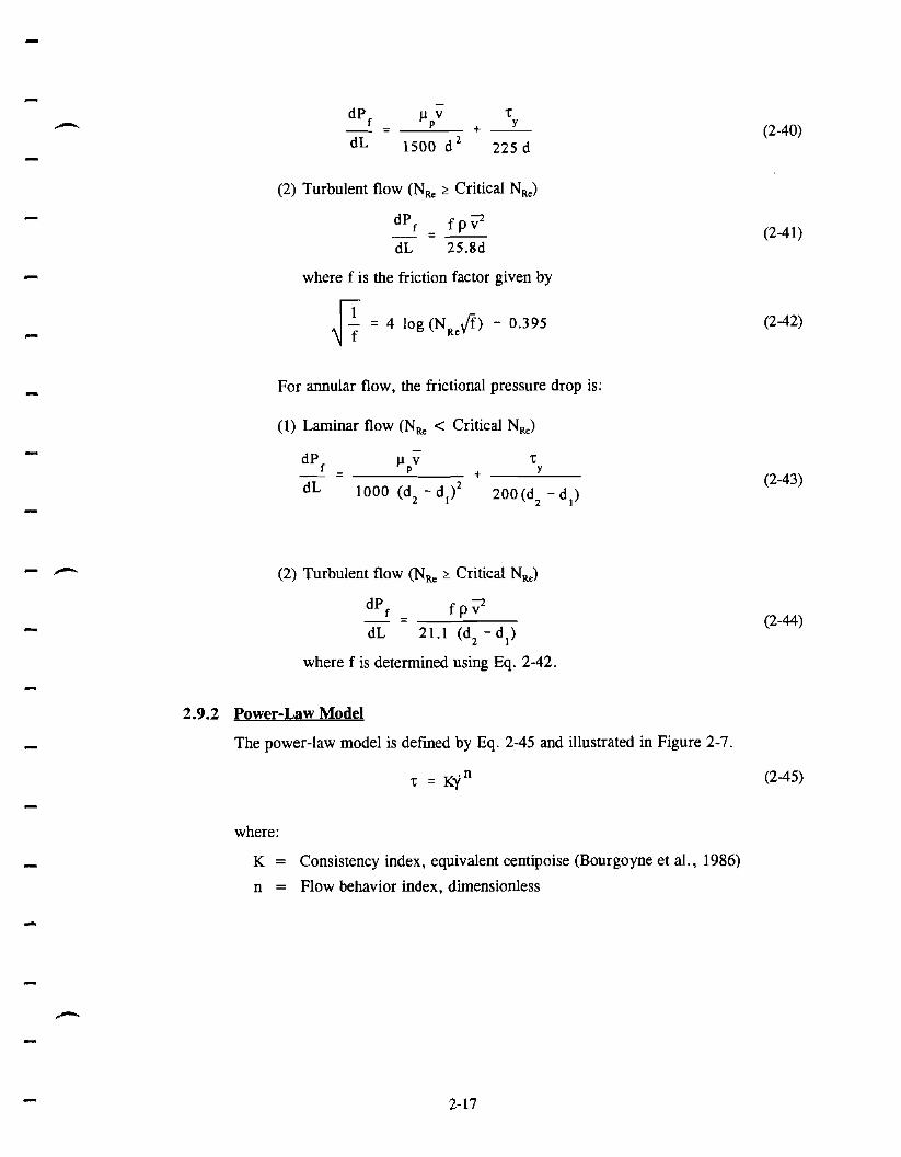
For annular flow, the frictional pressure drop is:

(1) Laminar flow (N, < Critical N,)

(2) Turbulent flow (N,, > Critical N,3

where f is determined using Eq. 2-42.

2.9.2 Power-Law Model

The power-law model is defined by Eq. 2-45 and illustrated in Figure 2-7.

t = K ~ " (2-45)

where:

K = Consistency index, equivalent centipoise (Bourgoyne et al., 1986)

n = Flow behavior index, dimensionless

Figure 2-7. Shear Stress Vs. Shear Rate for a Power-Law Fluid (Bourgoyne et al., 1986)

The fluid properties n and K are calculated as follows:

'600 n = 3.32 log- '300

The critical Reynolds number must be determined before the frictional pressure drop

can be calculated.

1. Mean Velocity

For pipe flow:

For annular flow: - v =

Q 2.448(d: - d:)

.u xapy JolAeqaq

MOD ua~!% e JOJ 8-z aln8!d mo13 peal aq m3 laqmnu sp~ouLaa le3!1!13 a q i

JaqurnN sp~ouLaa 1e3!1!13 'E

SP'O < u 103 0002 = "N le3!1!13

(6P-Z) sv.0 7 u s z .0 JOJ u 0088 - 096s = "N Ie3!1!13 Z'O > U 103 OOZV = "N 1~3!1!13

:(0661 "Ie la oga?) %ymollo~ a y Lq pa~em!xo~dde aq m3 8-z am%y u! mep a q i

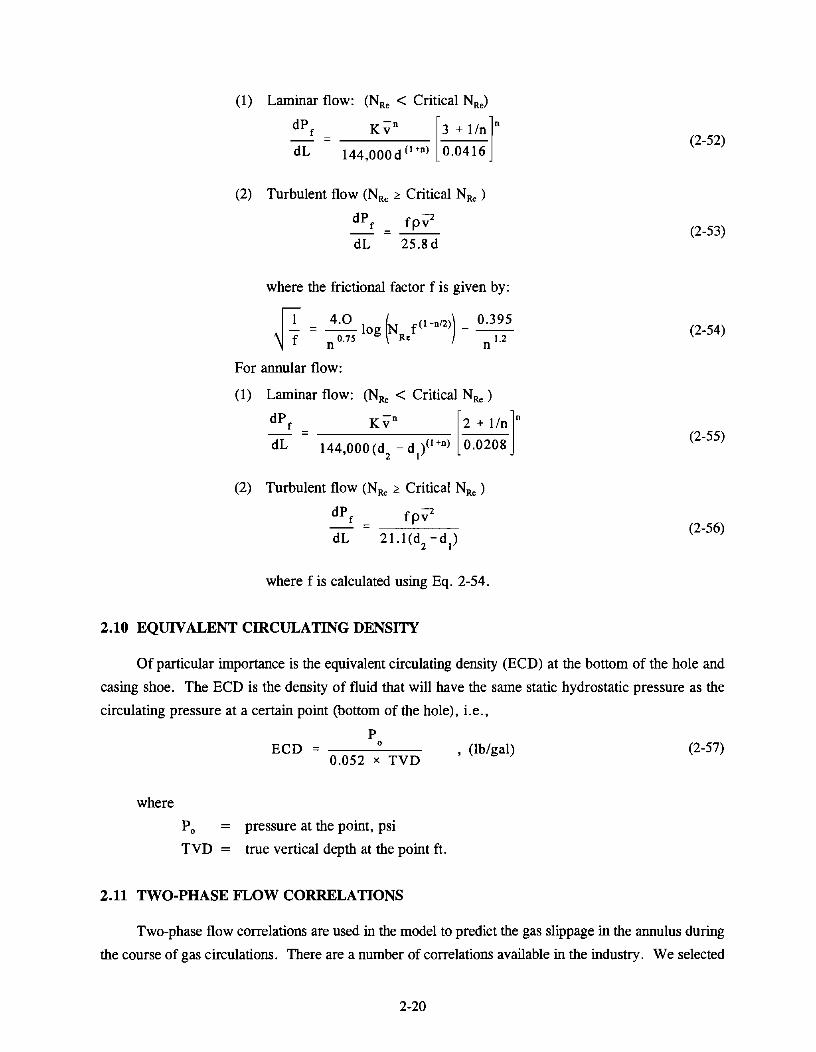
(1) Laminar flow: (N,, < Critical N,,)

(2) Turbulent flow (N,, 2 Critical N, )

where the frictional factor f is given by:

For annular flow:

(1) Laminar flow: (N, < Critical N,, )

(2) Turbulent flow (N, z Critical NRe )

where f is calculated using Eq. 2-54.

2.10 EQUIVALENT CIRCULATING DENSITY

Of particular importance is the equivalent circulating density (ECD) at the bottom of the hole and

casing shoe. The ECD is the density of fluid that will have the same static hydrostatic pressure as the

circulating pressure at a certain point (bottom of the hole), i.e.,

P ECD =

0.052 x TVD , (lb/gal)

where

Po = pressure at the point, psi

TVD = true vertical depth at the point ft.

2.11 TWO-PHASE FLOW CORRELATIONS

Two-phase flow correlations are used in the model to predict the gas slippage in the annulus during

the course of gas circulations. There are a number of correlations available in the industry. We selected

three of them for this well-control program. The following correlations use SI units. The Dressure d r o ~

s s h units before being used in Ea. 2-1 1.

2.11.1 Begas-Brill Correlation ( B e ~ e s and Brill. 1973)

This empirical correlation was developed from air-water two-phase flow experiments. It

applies to pipes of all inclination angles. The following is the procedure to calculate the liquid holdup:

(1) Calculate total flux rate

v m = "Sl + vsg

(2) Calculate no-slip holdup

sl 'ns =

vsl + vsg

(3) Calculate the Froude number, N,

(4) Calculate liquid velocity number

(5) To determine the flow pattern which would exist if flow were horizontal, calculate the correlating parameters, L,, L, L,, and L,:

(6) Determine flow pattern using the following limits:

Segregated:

<0.01 and NFR<L, ns

Transition:

AnS 20.01 and L2<NFR sL,

Intermittent:

0.01<Ans<0.4 and L,<N,, I L ,

or Ans 10.4 and L3<NFR <L4

Distributed: A <0.4 and NFR >L,

0s

or Ans10.4 and NFR>L4

(7) Calculate the horizontal holdup A,

where a, b, and c are determined for each flow pattern from the table:

Flow Pattern a b c

Segregated 0.98 0.4846 0.0868 Intennittent 0.845 0.5351 0.0173 Distributed 1.065 0.5824 0.0609

(8) Calculate the inclination correction factor coefficient.

where d, e, f, and g are determined for each flow condition from the table:

Flow Pattern d e f g

Segregated uphill 0.01 1 -3.768 3.539 -1.614 Intermittent uphill 2.96 0.305 -0.4473 0.0978 Distributed uphill No Correction C = O

All flow patterns downhill 4.70 -0.3692 0.1244 -0.5056

(9) Calculate the liquid holdup inclination correction factor

I) = 1 + c[sin(1.88) - 0.333 sin3(l.8e)]

where 8 is the deviation from horizontal axis.

(10) Calculate the liquid holdup A = AoI)

(1 1) Apply Palmer correction factor:

A = 0.918 -A for uphill flow A = 0.541 for downhill flow

(12) When flow is in transition pattern, take the average as follows:

where I, is the liquid holdup calculated assuming flow is segregated, I,

is the one assuming the flow is intermittent.

(13) Calculate frictional factor ratio

where

I ns and y = - 12

S becomes unbounded at a point in the interval 1 < y < 1.2; and for

y in this interval, the function S is calculated from

S = In ( 2 . 2 ~ - 1.2)

(14) Calculate frictional pressure gradient -

(NRs)ns - P n s ' ~ m ' d e l ~ n s

Use this no-slip Reynolds number to calculate no-slip friction factor using

Moody's diagram, f,'; then convert it into Fanning friction factor, f, = f,'14.

The two-phase friction factor will be

ftP f = f .- tp U s f

ns

The frictional pressure gradient is

NOTE: In the well-control model, it is assumed that when inclination angle is greater than 45", there is no slippage between gas and liquid.

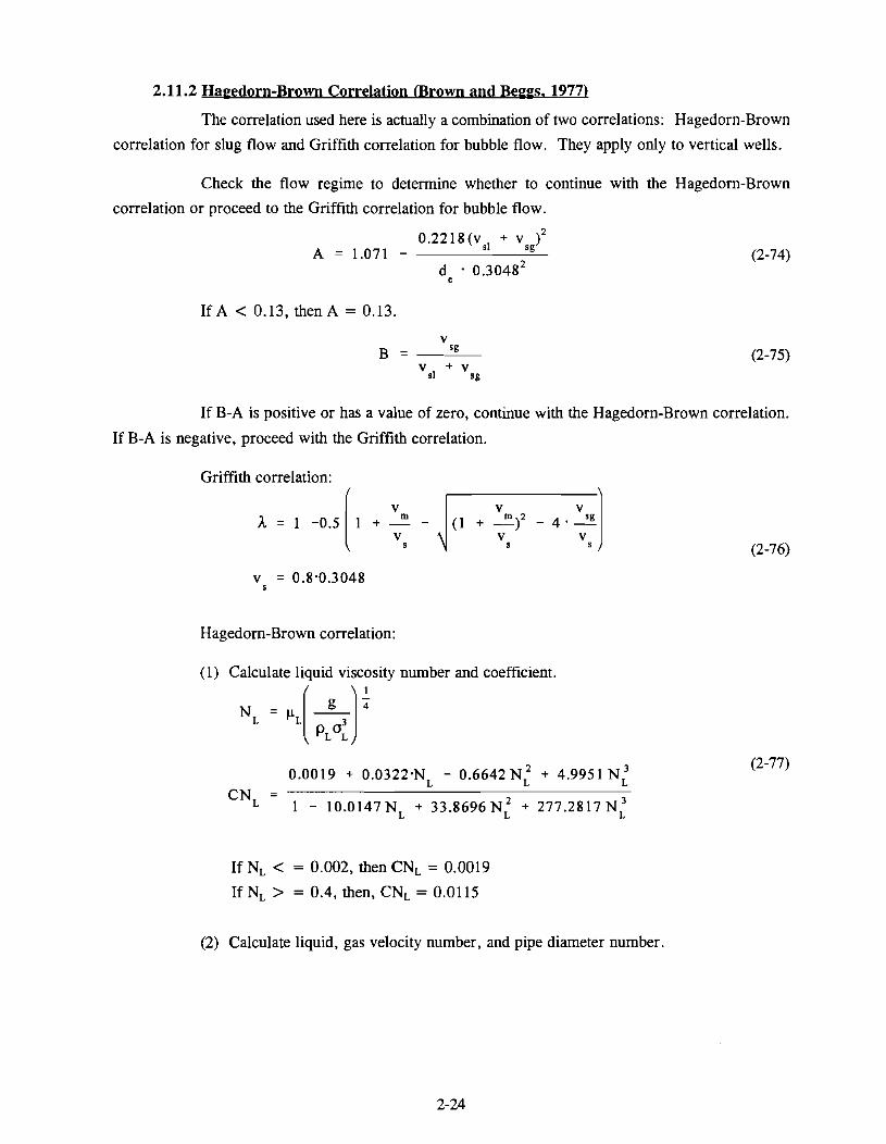
2.11.2 Hasedorn-Brown Correlation Brown and Beem. 19771

The correlation used here is actually a combination of two correlations: Hagedorn-Brown

correlation for slug flow and Griffith correlation for bubble flow. They apply only to vertical wells.

Check the flow regime to determine whether to continue with the Hagedorn-Brown

correlation or proceed to the Griffith correlation for bubble flow.

If A < 0.13, then A = 0.13.

If B-A is positive or has a value of zero, continue with the Hagedorn-Brown correlation.

If B-A is negative, proceed with the Grifiith correlation.

Griffith correlation:

Hagedorn-Brown correlation:

(1) Calculate liquid viscosity number and coefficient. / \ 1

0.0019 + 0.0322.NL - 0.6642 N: + 4.9951 N,' CN, =

1 - 10.0147NL + 33 .8696~ : + 277 .2817~ :

If N, < = 0.002, then CNL = 0.0019

If N, > = 0.4, then, CNL = 0.0115

(2) Calculate liquid, gas velocity number, and pipe diameter number.

C N L

@ = %k NGV (A) O.I0 IT]

(3) Determine the secondary correction factor correlating parameter

(4) Calculate liquid holdup

(5) Calculate frictional pressure gradient. 2

2f.Pns'Vrn P,, (2) = dc . -

f p,

f = Fanning friction factor -

P,, - No -slip average of densities

pr = Slip average of densities

NOTE: The Hagedorn-Brown correlation applies only to vertical wells. However, in the well control program, it is assumed that gas flows at the same velocity as the liquid when inclination angle is greater than 45". As far as the sections where inclination angle is between 0 and 45", the Hagedorn-Brown correlation is still used as if the well were vertical.

2.11.3 Hasan-Kabir Correlation CHasan and Kabir. 19921

This correlation is a recent development in multiphase flow technology. It was established

based on the hydrodynamic conditions and experiment observations. It applies to flow in annulus of

inclination up to 80".

1. Flow pattern identification.

The flow occurs in four different patterns depending on the superficial velocities and

properties. Figure 2-9 shows a typical flow regime map for wellbores.

SUPERFICIAL GAS VELOCITY fm/s)

Figure 2-9. Typical Flow Regime Map for Wellbores

20 1 1 I I I - 10- " . E DISPERSED BU9BLE - * t 0 I - 0, w

BUBBLY TRANSITION

> 0 3

5 0.1 - 0 - -I

a) Boundary A: transition from bubbly flow to slug or chum flow

v = (0.429 vsl + 0.357 v S ) sine sg

4 0 - L e

0: deviation from horizontal axis.

A SLUG OR CHURN

: 0.01 - 2 V )

I I

b) Boundary B: transition from bubbly or slug flow to dispersed bubble

-

I

d =

I 10 100

i .725 + 4 . 1 5 ~

0.6 -0.4

2fv, (+) (<I

When d s dc and when superficial gas velocity stays on the left of Boundary C, the

flow is in dispersed bubble.

C) Boundary C: transition from slug to dispersed bubble.

Boundary D: transition from slug to annular flow.

2. Liquid holdup calculation.

For bubbly or dispersed bubble flow v

A = 1 - sg

1 . 2 ~ ~ + Vs

For slug or chum flow

(1 + H cos 8)'.2 (2-87)

For annular flow

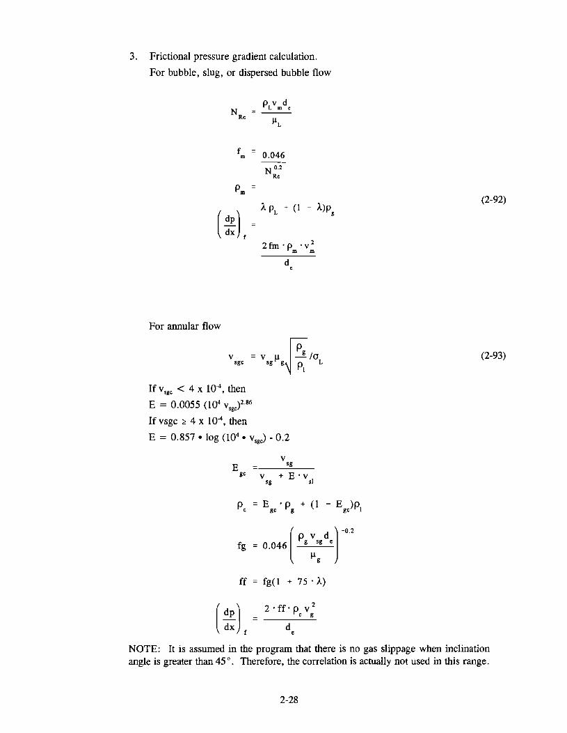
3. Frictional pressure gradient calculation.

For bubble, slug, or dispersed bubble flow

For annular flow 7

If v,,, < 4 x then

E = 0.0055 (lo4 v , , ) ~ . ~ ~

If vsgc 2 4 x lo4, then

NOTE: It is assumed in the program that there is no gas slippage when inclination angle is greater than 45 ". Therefore, the correlation is actually not used in this range.

3. Program Installation

3.1 BEFORE INSTALLING

3.1.1 Hardware and Svstem Reauirements

WELCON2 is written in Visual Basicm. It runs in either standard or enhanced mode of

Microsoft Windows 3.0 or higher. The basic requirements are:

Any IBM-compatible machine built on the 80286 processor or higher (with math co-

processor).

2 megabytes of RAM; 4 megabytes is recommended.

Hard disk.

Mouse.

CGA, EGA, VGA, 8514, Hercules, or compatible display. (EGA or higher resolution is recommended).

MS-DOS version 3.1 or higher.

8 Windows version 3.0 or higher in standard or enhanced mode.

These are the minimum system requirements. Due to the tremendous amount of - - calculations involved in WELCON2, we strongly recommend that WELCON2 be run on a 80386

processor or higher with math co-processor. At least four megabytes of RAM is highly recommended.

- To save memory space, a scheme of overlay is used in the program; that is, part of the program is loaded

into the memory when needed and unloaded from the memory when finished. To speed up this load or

unload process, we strongly suggest the program be installed on a hard drive and be operated from the

hard drive.

The amount of calculation (or calculation time) depends to a great extent on speed of the

machine and number of intervals used, which depends on the total length of the well and the length of

the calculation interval specified in PDI File. We have run the TEST files on the different machines we

have with different number of intervals. The results are tabulated in the following table. As can be seen

from the table, the calculation time increases by 3 to 4 times every time the length of the calculation

interval is halved. WELCON2 runs very slowly on a 80286 processor, especially the ones without math

co-processor.

NOTE: Math co-processor is present on all the machines. TEST files are used for these runs.

Options selected: Engineer's Method, Bingham-Plastic Model, water-based mud, Hasan-Kabir

correlation.

TABLE 3-1. Calculation Time Comparison

For assistance with the installation or use of WELCON2 contact:

Weiping Yang or Russell Hall Maurer Engineering Inc.

2916 West T.C. Jester Boulevard Houston, Texas 77018-7098 U.S.A.

Telephone: (7 13) 683-8227 Fax: (713) 683-6418

Calculation Interval (ft)

200

100

50

25

3.1.2 Check the Promam Disk

The program disk you received is a 3 %-inch, 1.44 MB disk containing twenty files. These

twenty files are as follows:

Number of Intervals

28

57

115

230

TIME: M1NUTES:SECONDS

80486 50 MHz (8 Meg)

00: 10

00:27

0 1 :26

04:41

80486 33 MHz (8 Meg)

00: 14

00:44

02: 17

07: 16

80386 25 MHz (4 Meg)

00:40

02:Ol

06:29

21 :09

SETUPKIT.DL- V B R U N ~ ~ ~ . D L - VER. DL- COMMDLG. DLL GSWDLL.DLL GSW.EXE SETUP.EXE SETUPI .EXE WELCON2.EXE SETUP. LST TEST. SDI TEST. WT 1 TEST.WPI TEST. PIT CMDIALOG .VBX GAUGE .VBX GRAPH.VBX GRID.VBX MDICHILD.VBX

We recommend that all .VBX and .DLL files that have the potential to be used by other

- DEA-44/67 Windows application be installed in your Microsoft WINDOWS\SYSTEM subdirectory.

This applies to all the .VBXs and .DLLs included here. The WELCON2 executable (WELCON2.EXE)

- fde should be placed in its own directory (default "C:\WELCON2") along with the example data files

TEST.W*IS. All these procedures will be done by a simple setup command explained in Section 3.2.

- F. In order to run WELCON2, the user must install all the fdes into the appropriate directory

on the hard disk. Please see Section 3.2 to setup WELCON2.

- It is recommended that the original diskette be kept as a backup, and that working diskettes

be made from it. - 3.1.3 Backuu Disk

It is advisable to make several backup copies of the program disk and place each in a - different storage location. This will minimize the probability of all disks developing operational

problems at the same time. - The user can use the COPY or DISKCOPY command in DOS, or the COPY DISKETTE

on the disk menu in the File Manager in Windows. - - 3.2 INSTALLING WELCON2

The following procedure will install WELCON2 from the floppy drive onto working - subdirectories of the hard disk (i.e., copy from A: drive onto C: drive subdirectory WELCON2 and

. WINDOWS \SYSTEM).

1. Start Windows by typing "WIN" <ENTER > at the DOS prompt.

2. Insert the program disk in drive B:\.

3. In the F i e Manager of Windows, choose Run from the File menu. Type B:\setup and press Enter.

4. Follow the on-screen instructions.

This is all the user needs to setup WELCON2. After setup, there will be a new Program Manager

Group which contains the icon for WELCON2 as shown in Figure 3-1.

I r m & &ELPATHSO D D R 4 G 8 2 m M 0 0 3 0 BUWE, DRIFE~

~ W H f Q l ~ s i r c r s l CTUFE2 ~ l l ax l Rd AFE

Figure 3-1. DEA APPLICATION GROUP Window Created by Set Up

3.3 STARTING WELCON2

3.3.1 Start WELCON2 from Group Window

To run WELCON2 from Group Window, the user simply double-clicks the "WELCON2"

icon, or when the icon is focused, press <ENTER > .

3.3.2 Use Command-Line Option from Windows

In the Program Manager, choose _Run from the File menu. Then type

C:\WELCON2\WELCON2.EXE < ENTER > .

- 3.4 ALTERNATIVE SETUP

When SETUP procedure described previously fails, follow these steps to install the program:

1. Create a subdirectory on drive C: C:\WELCONZ.

2. Insert source disk in drive B: (or A:).

3. Type: C:\WELCONZ <ENTER>.

4. At prompt C:\WELCONZ, type:

Copy B:\WELCONZ.EXE <ENTER > Copy B:\TEST.* <ENTER>.

5. Type: CD C:\WINDOWS <ENTER>

6. At prompt C:\WINDOWS, type:

Copy B:\VBRUNlOO.DL_ VBRUN100.DLL <ENTER >

7. Type: CD SYSTEM.

8. At prompt C:\WINDOWS\SYSTEM, type:

Copy B:\*.DLL <ENTER>

Copy B:\GSW.EXE <ENTER > Copy B:\*.VBX < ENTER > .

9. Type: CD.. <ENTER > then key in "WIN"' <ENTER > to start Windows 3.0 or later

version.

10. Click menu "File" under "PROGRAM MANAGER," select item "New ...," click on

"PROGRAM GROUP" option, then [OK] button.

1 1. Key in "DEA APPLICATION GROUP after label "Description: ," then click on [OK] button.

A group window with the caption of "DEA APPLICATION GROUP" appears.

12. Click on menu "File" again, Select "NEW ...," click on "PROGRAM ITEM" option, then,

[OK] button.

13. Key in "WELCONZ" after label "Description," key in "C:\WELCONZ\WELCONZ.EXE

after label "COMMAND LINE," then click on [OK] button. The WELCONZ icon appears.

14. Double click the icon to start the program.

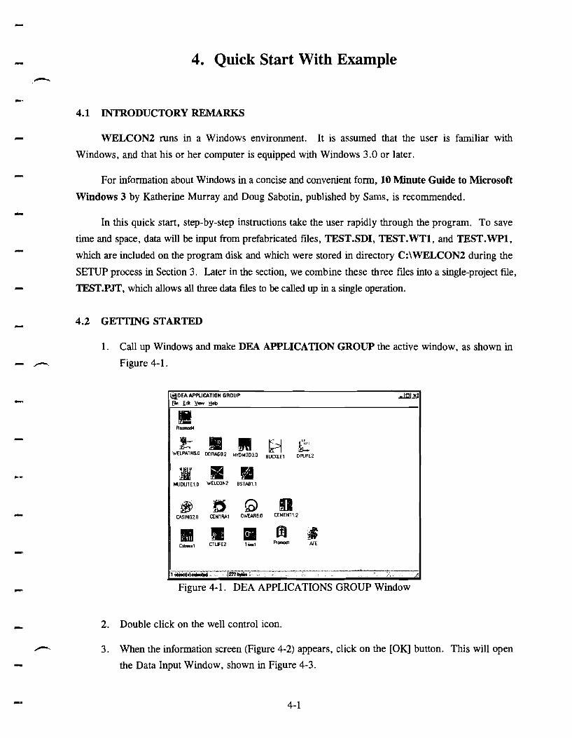
4. Quick Start With Example

4.1 INTRODUCTORY REMARKS

WELCONZ runs in a Windows environment. It is assumed that the user is familiar with

Windows, and that his or her computer is equipped with Windows 3.0 or later.

For information about Windows in a concise and convenient form, 10 Minute Guide to Microsoft

Windows 3 by Katherine Murray and Doug Sabotin, published by Sams, is recommended.

In this quick start, step-by-step instructions take the user rapidly through the program. To save

time and space, data will be input from prefabricated files, TEST.SD1, TEST.WT1, and TEST.WP1,

which are included on the program disk and which were stored in directory C:\WELCONZ during the

SETUP process in Section 3. Later in the section, we combine these three fdes into a single-project file,

TEST.PJT, which allows all three data files to be called up in a single operation.

4.2 GETTING STARTED

1. Call up Windows and make DEA APPLICATION GROUP the active window, as shown in

Figure 4-1.

I l W 4 - IW- b

Figure 4-1. DEA APPLICATIONS GROUP Window

2. Double click on the well control icon.

3. When the information screen (Figure 4-2) appears, click on the [OK] button. This will open

the Data Input Window, shown in Figure 4-3.

WELL CONTROL PROGRAM lrerrbn 2.11 - x

WELL CONTROL PROGRIIM lvcrsion 2.11

DEA-441DEPr67 Projed to Develop And Evaluate Horizontal

Drllllng Technology And

Projed to Develop And Evaluate Slim+lole And Coiled-Tubing Technology

BY Maurer Enqinecrinq Inc.

This corvriahted 1993 confidential reoort and comruter Drosram are for ih; A l e use of Participants on the Drilling Engineering Aasoclatlon DEA-44 and/or DEA-67 Proleets and thelr affiliates. and are not to be disclosed to other pa'rt~es. Data output from the program can be disclosed to the third parties. Participants and their affiliates are free to makc copies of this report and program for thelr in-house use only.

Maurer Englneerlng I n r mates no warranly or representation. either exprkssed o; implied. with respect tb the program or documentation, Including their qualily, perlormance. merchb nablllly, or fitness for a particular pu~pose.

Figure 4-2. Disclaimer

Figure 4-3. Main Menu: Data Input Window

4. When the Data Input Window, Figure 4-3, appears, notice that there are five sets of choices

h to be made in this Data Input window. These are:

1. Kill Procedure - Driller's or Engineer's Method;

2. Rheology Model - Power-Law or Bingham Plastic Model;

3. Mud Base - Water-Based or Oil-Based Mud;

4. Two-Phase Flow Correlation - Single Bubble, Beggs and Brill, Hagedorn-Brown, or

Hasan-Kabir; and

5. Units of Measure - English or Metric.

The user's decision is made by clicking on the button in front of each listed option. Decisions can

be made any time before running the program.

If not using the mouse, move the cursor from one decision field to another by using the tab key.

Move within a decision field by using the arrow keys.

5. After setting these five options, click on SDI in the menu bar at the top of the screen. This

will open the Survey Data Input window, shown in Figure 4-4.

~ ~ - S U A M Y DATA INPUT ISDI) =El?. 1

Figure 4-4. Survey Data Input Window

If not using a mouse, activate the menu bar with the < ALT > key. Use arrow keys to move along

F - the menu bar. Use <ENTER> key to make selection. - 6. When the Survey Data Input window opens, click on File as shown in Figure 44 . This will - open the File window, shown in Figure 4-5.

Figure 4-5. File Selection Window

When the File window opens, click on Open. This will open the SDI File Open window,

shown in Figure 4-6.

Figure 4-6. File Window

When the SDI File Open window opens, click on C:\ in the Drive box. This will cause the

of *.SDI files stored in drive C:\WELCON2\ to appear in the File Name box at the upper left of

window, as shown in Figure 4-6. Now, click on Test.SD1, then click on [OK]. This will open

Survey Data Input Window, and fill it with data, as shown in Figure 4-7.

list

the

the

Figure 4-7. Survey Data Input Window-Filled

C . Before leaving the Survey Data Input window, notice the three sets of options which are available.

These are:

- 1. Depth - Feet or Meters;

2. Inclination - Decimal degrees or Degrees and Minutes; and

- 3. Azimuth - Angular or Oil Field Measure.

To change any of these, click on the desired option. If not using a mouse, use the tab key to move

- from one field to another, and use the arrow keys to move within a field. As the user moves from one

value to another, the highlight will move accordingly. Default choices are Feet, Decimal, and Angular,

..- respectively.

Before leaving this Survey Data Input window, set these three options to suit your needs.

8. Now, click on File on the menu bar above the Survey Data Input window. When the File

window opens, as shown in Figure 4-8, click on Exit.

1;s-SURVEY DATA INPUT-C:\WELCONZ\TEST.SDI U A ~

Figure 4-8. Back to File Selection Window

This will bring back the Input Data Window with the SDI Filename box now listing

C:\WELCON2\TEST.SDI, as shown in Figure 4-9.

1 Fad SDI TDI POI R u l OulPul Heb 1

Figure 4-9. Input Data Window

4-6

10. Click on TDI on the menu bar at the top of the window. This will open the Tubular Data

Input window, shown in Figure 4-10. All data spaces in this window are blank.

I*-TUBUUR DATA INPUT (TDII- A A ~

Figure 4-10. Tubular Data Input Window

11. Click on File at the upper left of this window. This will open the File windows.

12. Click on Open in this window. This will open the TDI Fie Open window.

13. Click on Test.WT1 and then on [OK] in this window.

14. This will reopen the Tubular Data Input Data Input window and fill it with numerical data,

as shown in Figure 4- 1 1.

i j8-TUEUlAFl DATA INPUT (TDIJC:\WELCDNZ\TEST.WTl ~ A I

Figure 4-1 1. Tubular Data Input Window-Filled

Then click on Fie at the left end of the menu bar.

When the File window opens, click on Exit.

This will reopen the Data Input Widow, and add the title C:\WELCONZ\TEST.WTl to

the TDI Fie name box, as shown in Figure 4-12.

Figure 4-12. Data Input Window

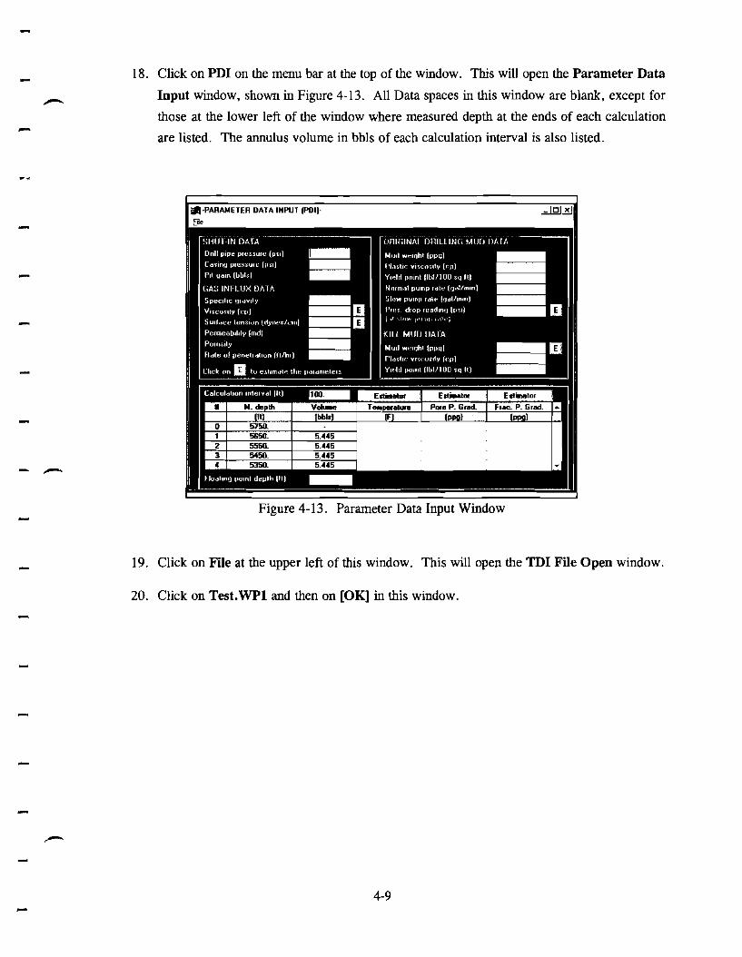
18. Click on PDI on the menu bar at the top of the window. This will open the Parameter Data

Input window, shown in Figure 4-13. All Data spaces in this window are blank, except for

those at the lower left of the window where measured depth at the ends of each calculation

are listed. The annulus volume in bbls of each calculation interval is also listed.

a-PARAMETEA DATA INWT IPDII-

Figure 4-13. Parameter Data Input Window

19. Click on File at the upper left of this window. This will open the TDI F i e Open window.

20. Click on Test.WP1 and then on [OK] in this window.

This a

in Fig1

.al data, as

Figure 4-14. Parameter Data Input Window-Filled

There are a number of user inputs and options in the Parameter Data Input window. These

choices have all been made and incorporated into the Test.WP1 file to expedite the execution of this

example run. The Parameter Data Input will be discussed in the next section of this manual.

22. Click on FiIe at the left end of the menu bar. When the Fie window opens, click on Exit.

This will return to the Input Data window, as shown in Figure 4-15.

I F~le SDI TDI PDI Run Oulh! Hclo I

Figure 4-15. Data Input Window

4-10

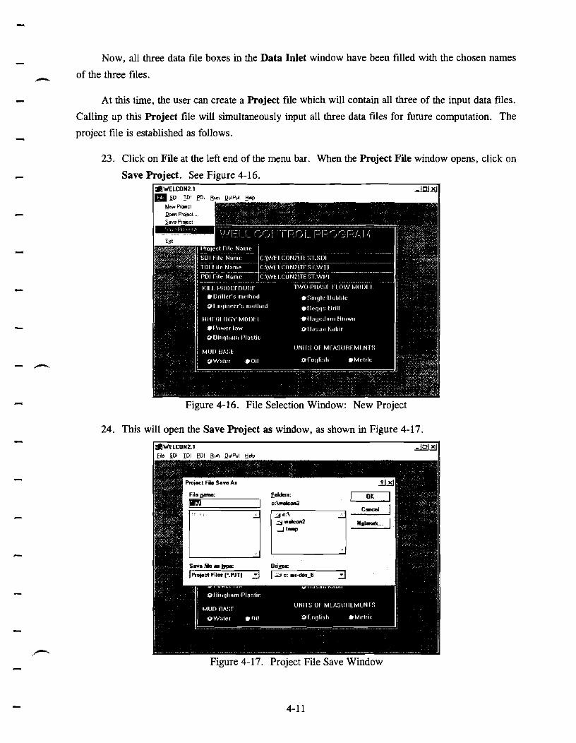
- Now, all three data file boxes in the Data Inlet window have been filled with the chosen names

h of the three files.

- At this time, the user can create a Project file which will contain all three of the input data files.

Calling up this Project file will simultaneously input all three data files for future computation. The

- project file is established as follows.

23. Click on Fie at the left end of the menu bar. When the Project Fie window opens, click on

Save Project. See Figure 4-16.

Figure 4-16. File Selection Window: New Project

24. This will open the Save Project as window, as shown in Figure 4-17.

Figure 4-17. Project File Save Window

4-1 1

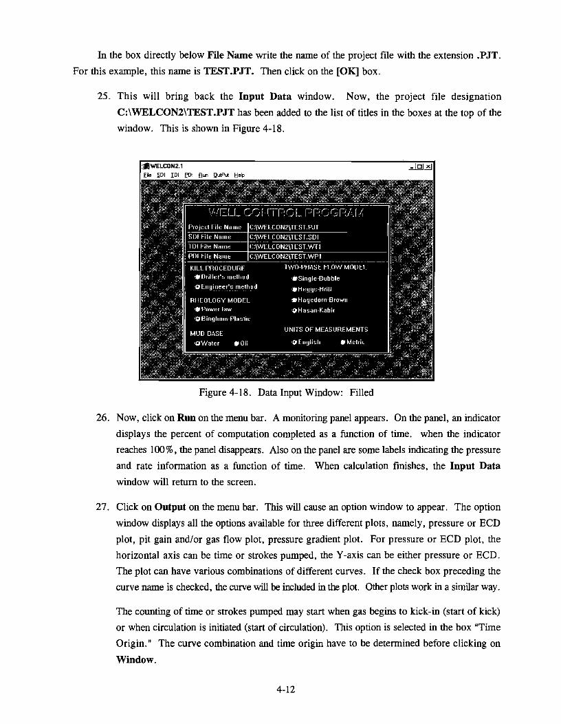
In the box directly below F i e Name write the name of the project file with the extension .PJT.

For this example, this name is TEST.PJT. Then click on the [OK] box.

25. This will bring back the Input Data window. Now, the project file designation

C:\WELCON2\TEST.PJT has been added to the list of titles in the boxes at the top of the

window. This is shown in Figure 4-18.

Figure 4-18. Data Input Window: Filled

26. Now, click on Run on the menu bar. A monitoring panel appears. On the panel, an indicator

displays the percent of computation completed as a function of time. when the indicator

reaches 100%, the panel disappears. Also on the panel are some labels indicating the pressure

and rate information as a function of time. When calculation finishes, the Input Data

window will return to the screen.

27. Click on Output on the menu bar. This will cause an option window to appear. The option

window displays all the options available for three different plots, namely, pressure or ECD

plot, pit gain andlor gas flow plot, pressure gradient plot. For pressure or ECD plot, the

horizontal axis can be time or strokes pumped, the Y-axis can be either pressure or ECD.

The plot can have various combinations of different curves. If the check box preceding the

curve name is checked, the curve will be included in the plot. Other plots work in a similar way.

The counting of time or strokes pumped may start when gas begins to kick-in (start of kick)

or when circulation is initiated (start of circulation). This option is selected in the box "Time

Origin." The curve combination and time origin have to be determined before clicking on

Window.

S W E L L CONTROL PROGRAM -OUTPUT ad1

a Mas. ECD Mona Walbara

a Frsc. Pms.ue Gra&nt

Figure 4-19. Output Option Window

28. Click on Widow on the menu bar. This opens the Graphic Output window, shown in

Figure 4-20. The first three items are for the arrangement of a group of child windows.

They can be used only when there is at least one child window on the screen. The other five

items are different child windows. Clicking on any one of them will bring out the

corresponding child window. The child window "Tabulated Results" always displays the

tabulated results for Active Graph Child Window.

R Pit Gak

P i Gsr Flow Rae

B Max ECO Abnp Wdlbare

[il Ftsc. P~e*.me Gr&d

Figure 4-20. Output Format Window

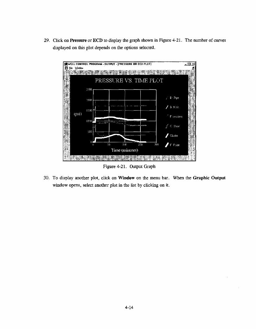
29. Click on Pressure or ECD to display the graph shown in Figure 4-21. The number of curves

displayed on this plot depends on the options selected.

Figure 4-2 1. Output Graph

30. To display another plot, click on Window on the menu bar. When the Graphic Output

window opens, select another plot in the list by clicking on it.

will

3 1 . After viewing several of the graphs, they may be presented in a multiple display, as shown

in Figures 4-22 and 4-23. Figure 4-22 is generated by clicking on Cascade in the Graphic

Output window.

IJ)WELL CONTROL PROGRAM -OUTPUT

Figure 4.

not be det

Figure 4-22. Cascade Window

:rations, and

Figure 4-23. Tile Window

4-15

32. To print any of the screen displays, click on F i e at the left end of the menu bar. When the

F i e window opens, click on Print. Figure 4-24 is the printed output of the Choke Pressure

graph.

Figure 4-24. Full Size Plot

33. To leave the graphic displays, click on File at the left end of the menu bar. When the File

window opens, click on Exit. This will return the user to the Input Data window.

34. The Help option at the right end of the menu bar will open the Help window. The two

options available in this window are Assistance and About.. . Clicking on Assistance will

open the window shown in Figure 4-25, which gives phone and FAX numbers and

individuals to contact for assistance with the program.

Figure 4-25. Help Window

Clicking on About.. in the Help window opens a window with infoxmation about the program,

and a listing of the equipment you are using to run the program.

35. To leave the program, click on F i e on the menu bar. When the File window opens, click

on Exit.

5. Options and Choices of the Model

5.1 INPUTDATA

There are five choices to be made in the Input Data window, shown in Figure 5-1.

Figure 5-1. Input Data Window

1. Kill procedure. Either Driller's or Engineer's method.

A. In the Driller's method, mud weight is not increased as the kick is circulated out. At

the end of this procedure, there is still pressure at both the drill pipe and choke.

B. In the Engineer's method, the well is shut in and the mud weight necessary to kill the

well is determined. The mud weight is raised to this value, and the kick is circulated

out. At the conclusion of this process, both drill pipe and choke pressure are

atmospheric when circulation stops.

2. Rheology Model. Either Power-Law or Bingharn Plastic.

Either of these models will give essentially the same results over the dynamic range used

in the kill procedure. Most field measurements assume the Bingharn plastic model, although there are - conversions available to express Fann V.G. readings in terms of the power-law constants. If the pressure - drop measured at slow pump rate is input (Parameter Data Input), a correction factor will be applied

+ to the friction drop calculated for mud flow. This should greatly reduce any error resulting from the

choice of flow model.

3 . Two-Phase Flow Model.

Here the user is on his or her own. The choice of multiphase correlation model is a matter

of experience or intuition. A number of the inputs required for the Beggs and Brill, Hasan-Kabir, and

Hagedorn and Brown models are not measurable, and must be estimated by the user. The single-bubble model

yields the highest choke pressure, and may be considered to represent the worst possible scenario.

4. Metric or English. Either set of units can be accommodated by the program.

5.2 SDI AND TDI DATA INPUTS

Input to these two data files is straightforward, and will not be elaborated here.

5.3 PARAMETER DATA INPUT

The Parameter Data Input window is shown in Figure 5-2.

*-PARAMETER DATA INPUT p n l l - A ~ i l

Figure 5-2. parameter D ~ I I I ~ U ~ Window

Starting down the left-side column, the first four items must be supplied by the user, i.e.,

1. Drill-pipe pressure,

2. Casing pressure,

3. Pit gain, and

4. Specific gravity of gas. (air = 1.00)

5 . Viscosity, can either be supplied by the user, or, if the user chooses to click on m], the

program will use the formation pressure and temperature, and the gas specific gravity to

calculate the gas viscosity.

6. Surface tension of the mud, may either be entered by the user, or, if the user clicks on w], a default value of 80 dyneslcm will be supplied. This is the surface tension of clean water.

It is required in some of the multiphase correlations.

7. User must enter permeability, porosity and rate of penetration. These parameters will be

used in the calculation of gas influx rate.

8. Starting down the right column, items #lo, #11, and #12 are, respectively, mud weight,

plastic viscosity, and yield point of the original density mud. The user must supply these.

9. Normal pump rate is the pump rate before shut-in. It must be supplied by the user.

10. Pump pressure may be supplied by the user. Pressure is determined by the slow pump rate

and slow pumping test. This value will be compared with the frictional pressure drop

calculated using the mud properties in items #lo, #11, and #12, and the flow path geometry

listed in the Tubular Data Input. A correction factor will be determined from this

comparison. This factor will be used to correct the friction pressure drop computed for the

single-phase mud flow to agree with that observed in the slow pump rate test.

If the user elects to click on the [El, the program will calculate a frictional pressure drop for the

mud flow, and place it in this box.

The program will calculate the mud weight of the kill mud when the user clicks on w] for item

#16. Items #17 and #18, kill mud plastic viscosity and yield point, must be supplied by the user.

After entering the data for example, the top of the Parameter Data Input is shown in Figure 5-3.

a-PARAMETER DATA INPUT [PDII-C:\WELCONZ\TEST.WPl &A

Figure 5-3. Parameter Data Input Window: Partially Filled

The three empty columns at the bottom of the window must now be filled.

Click on the [Estimator] button of the Temperature column to open the Temperature

Estimation window, as shown in Figure 5-4.

a-PARAMETER DATA INPUT WDII-C\WELUINZ\TEST.WPI a 4

Figure 5-4. Temperature Data Window

5-4

- Enter surface temperature and temperature gradient in degrees FI100 ft or in degrees Cl30 meters)

,- and click on the [Accept] button to enter the temperature readings into the temperature column in the - Parameter Data Input window, as shown in Figure 5-5.

a-PAWMETER DATA INPUT IPDltC:\WEUONATEST.WPI d z !

- Enter surface temperature and temperature gradient in degrees F/100 ft or in degrees C/30 meters)

h and click on the [Accept] button to enter the temperature readings into the temperature column in the - Parameter Data Input window, as shown in Figure 5-5.

1s-PWETER DATA INPUT IPDII-C:\WELCONXTEST.WPI & I J ~

I I

Figure 5-5. Temperature Data Entered

- Individual entries in these three columns (Temperature, Pore P. Grad., and Frac. P. Grad.)

may be edited or added by clicking onto them and typing in the desired change. - The Calculation Interval is also a user input, and is edited by clicking onto the box and entering

the desired change. - In a similar manner, the PORE PRESSURE GRADIENT window and the FRACTURE

PRESSURE GRADIENT are opened, filled, and the results entered into the Parameter Data Input - window. These two windows are shown in Figures 5-6 and 5-7.

~ l s 3 l \ r ~ 0 1 1 3 M \ ~ ~ l a d l I M N I VlVQ t l31311VWd-~

The c

Figure 5-8. Filled Parameter Data Input Window

. r

In this window, the pump pressure (300 psia) was user input. Clicking the B] button on the

Pump Pressure line will replace the user input value with a calculated value, 340.05, as shown in

Figure 5-9.

Figure 5-9. Calculated Pump Pressure

5-7

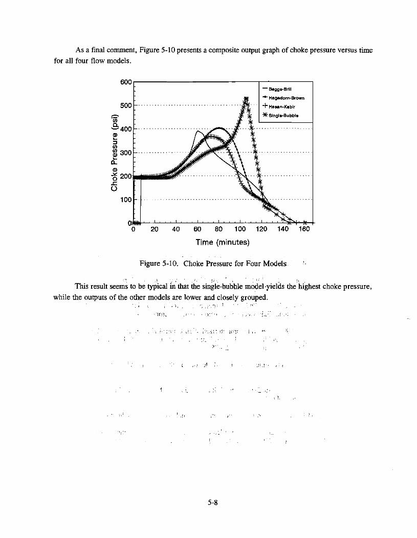
As a final comment, Figure 5-10 presents a composite output graph of choke pressure versus time for all four flow models.

- Hagadorn-Brown

. . . . . . . . . . . . . . . . . . . . . . . . . . . . . . . . . . .

. . . . . . . . . . . . .

0 20 40 60 80 100 120 140 160

Time (minutes)

Figure 5-10. Choke Pressure for Four Models

, .. . , . .

This result seems to be G ica l &that the s i n i l e - b u b ~ model.yields &=highest choke pressure,

while the outputs of the other models are lower and closely grouped. , - . : . ? . . . .

..I i , * I , , . . : , . . .I(>!. , . , : ' . , , .:;-,.; ! . - . ;..A . : ' , , , '

6. References

Barnes, D., 1987: "A Unified Model for Predicting Flow-Pattern Transitions for the Whole Range of Pipe Inclinations," International Journal Multiphase Flow, Vol. 13, No. 1 , pp. 1-12.

Beggs, H.D. and Brill, J.P., 1973: "A Study of Two-Phase Flow in Inclined Pipes," Journal of Petroleum Technology, May.

Bourgoyne, A.T., Jr., et al., (Date Unknown): Applied Drilling Engineering, Richardson, Texas, Society of Petroleum Engineers.

Brill, J.P. and Beggs, H.D., 1991: Two-Phase Flow in Pipes, Sixth Edition, January.

Brown, K.E. and Beggs, H.D., 1977: "The Technology of Artificial Lift Methods," Vol. 1 , Published by Pennwell Books.

Caetano, E.F., Shoharn, 0. and Brill, J.P., 1992: "Upward Vertical Two-Phase Flow Through an Annulus - Part I: Single-Phase Friction Factor, Taylor Bubble Rise Velocity, and Flow Pattern Prediction," Journal of Energy Resources Technology, Vol 114, March.

Caetano, E.F., Shoham 0. and Brill, J.P., 1992: "Upward Vertical Two-Phase Flow Through an Annulus - Part 11: Modeling Bubble, Slug, and Annular Flow," Journal of Energy Resources Technology, Vol 114, March. * . ,

Hasan, A.R. and Kabir, C.S., 1992: "Two-Phase Flow in Vertical and Horizontal Annuli," Int. J. Multiphase Flow, Vol. 18, No. 2, pp. 279-293. II %

, LeBlanc, J.L. and Lewis, R.L., 1967: "A Mathematical Model of a Gas Kick," SPE Paper 1860 presented at SPE 42nd Annual Fall Meeting, Houston, Texas, October 1-4.

Leitiio, H.C.F. et al., 1990: "General Computerized Well Control Kill Sheet for Drilling Operations with Graphical Display Capabilities," SPE 20327 presented at the Fifth SPE Petroleum Computer Conference held in Denver, Colorado, June 25-28.

Nickens, H.V., 1987: "A Dynamic Computer Model of a Kicking Well," SPE Drilling Engineering, June.

O'Brian, P.L., et al., 1988: "An Experimental Study of Gas Solubility in Oil-Based Drilling Fluids," SPE Drilling Engineering, March.

Santos, O.L. A., 199 1 : "Well-Control Operations in Horizontal Wells," SPE Drilling Engineering, June.

Santos, O.L.A., 1991: "Important Aspects of Well Control for Horizontal Drilling Including Deepwater Situations," SPEIIADC Paper 21993 presented at 1991 SPE/IADC Drilling Conference, Amsterdam, March.

Specification for Materials and Testing for Well Cements, 1990: API SPECIFICATION 10 (SPEC 10) Fifth Edition, July 1 .

Van Slyke, D.C., Huang E.T.S., 1990: "Predicting Gas Kick Behavior in Oil-Based Drilling Fluids Using a PC-Based Dynamic Wellbore Model," IADCISPE Paper #19972, presented at the 1990 IADCISPE Drilling Conference held in Houston, Texas, February.

White, D.B. and Walton, I.C., 1990: "A Computer Model for Kicks in Water- and Oil-Based Muds," IADCISPE Paper 19975 presented at the 1990 IADCISPE Drilling Conference, Houston, Texas, February 27-March 2.