well control procedures and simulations · procedures rely on a set of simplifying assumptions....
TRANSCRIPT

Faculty of Science and Technology
MASTER’S THESIS
Study program/ Specialization:
Petroleum EngineeringSpring semester, 2011
Open
Writer:Harald Frette Litlehamar …………………………………………
(Writer’s signature)Faculty supervisor: Professor Kjell Kåre Fjelde
External supervisor(s): Helge Saure (Transocean)
Title of thesis:
Well Control Procedures and Simulations
Credits (ECTS): 30
Key words:- Well control- Kick- Kick simulator- AUSMV
Pages: 97
+ enclosure: 20
Stavanger, June 15th 2011Date/year

Well Control Procedures and Simulations2Abstract
A brief introduction is given to a range of well control procedures. It was found that many of theprocedures rely on a set of simplifying assumptions. This is particularly true in the hand calculationsfor designing a well kill. This set of assumptions was used to define an analytical model. The premisesof the analytical model and some of the procedures were tested in a crude kick simulator. The mainobjective of this thesis was to verify some of the well control procedures, and to shed light on theirlimitations. Particular attention was given to driller’s method for a vertical and horizontal well.Additionally, simulations were run to investigate the worst case scenarios which a well might besubjected to if well control is lost.
As a means for achieving this, the previously implemented explicit numerical AUSMV scheme wasused as a basis for simulations on a kicking well. However, in order to conduct realistic simulationssome modifications to the scheme had to be introduced. The most important modification was theimplementation of a PI-regulator, as it proved impossible simply to set the bottomhole pressure to adefined constant value in the numerical scheme. Extensive tuning of the regulator was necessary forit to perform satisfactory. In this process, a novel alternative to the classical PI-regulator wasdiscovered.
Further modifications deemed necessary:
Improved accuracy in reading of bottomhole and choke pressures. Implementation of additional topside parameters (pit gain, drillpipe pressure) A more realistic friction model. Changing the liquid component of the system from water to drilling fluid (altering the liquid
density). A chokeline and riser for simulation on subsea wells. Opening up for wellbore deviation. A Darcy relation for influx where influx size and mass rate depends on downhole pressure
differential. This is important for drilled kicks or connection kicks. Additionally, a choke model was implemented in the model, but it has not been used in the
simulations. The choke model depicts the backpressure as a function of fluid density, flowrate and choke opening.
By use of the crude kick simulator, simulations were run for a vertical and a horizontal well. Theresults obtained by the kick simulator were compared to hand calculations. The main discovery wasthat although the hand calculations produce slight errors, the errors exclusively functions asadditional safety margins with respect to downhole pressure differential.
It was also found that a gas bubble migrating in a shut-in annulus subjects the well to higher loadsthan the gas filled well scenario.

Well Control Procedures and Simulations3
AcknowledgementI would like to thank professor Kjell Kåre Fjelde for outstanding help and guidance in the work withmy thesis. He has kept his office door open at all times. Thank you for sharing your insight in the wellcontrol discipline, for helping out with Matlab programming and for being a great conversationpartner.
Further, I am very grateful to toolpusher Helge Saure and Transocean. He sent me to an IADC wellcontrol course, which was very helpful. I was also allowed to use Transocean’s well controlhandbook. He was also partially responsible for the subject of the thesis. “It is all about theprocedures,” he said.
Some of my friends at the university also require particular attention. Stian Molvik has been writing athesis on the theoretical aspects of the AUSMV scheme. Thank you for the inspiring discussions andfor enlightening me! Andreas Davidsen, Kim Øvstebø, Ørjan Tveteraas and Johan Helleren have beenkeeping me with company when working long hours at the university. Thank you!
Finally, I would like to thank my family for all help, support and patience along the way.

Well Control Procedures and Simulations4
Table of contents
Abstract ....................................................................................................................................... 2
Acknowledgement ....................................................................................................................... 3
Table of contents ......................................................................................................................... 4
1. Introduction.......................................................................................................................... 7
2. What is well control? ............................................................................................................ 8
2.1. The barrier philosophy............................................................................................................. 8
2.1.1. The primary barrier........................................................................................................10
2.1.2. The secondary barrier....................................................................................................10
2.2. Killing a well ...........................................................................................................................10
3. Kick prevention and preparation ......................................................................................... 11
3.1. Well design and planning.......................................................................................................11
3.1.1. Mud weight schedule ....................................................................................................12
3.1.2. Casing design .................................................................................................................12
3.1.3. Well design example......................................................................................................14
3.2. Preventive operational procedures .......................................................................................15
3.2.1. Tripping ..........................................................................................................................16
3.2.2. Drilling............................................................................................................................17
3.3. Procedures for well control preparedness ............................................................................18
3.3.1. Leak-off test ...................................................................................................................18
3.3.2. Slow circulating rate ......................................................................................................18
4. Kick detection ..................................................................................................................... 19
4.1. Kick indicators........................................................................................................................19
4.1.1. Increase in return rate and surface volumes.................................................................19
4.1.2. Increase in drillability.....................................................................................................19
4.1.3. Other drilling parameters ..............................................................................................20
4.1.4. Drilling fluid properties ..................................................................................................20
4.1.5. Cuttings geometry .........................................................................................................20
4.1.6. Increase in background gas ...........................................................................................20
4.1.7. Increase in temperature ................................................................................................20
4.1.8. Downhole measurements..............................................................................................21

Well Control Procedures and Simulations54.2. Flow check .............................................................................................................................21
5. Influx containment.............................................................................................................. 22
5.1. Hard shut-in ...........................................................................................................................22
5.2. Soft shut-in.............................................................................................................................22
6. Removal of influx fluid from the wellbore............................................................................ 23
6.1. Driller’s method .....................................................................................................................23
6.2. Wait & weight ........................................................................................................................24
6.3. Static volumetric method ......................................................................................................25
6.4. Bullheading ............................................................................................................................25
7. An analytical model ............................................................................................................ 26
7.1. Assumptions ..........................................................................................................................26
7.1.1. Conservation of mass.....................................................................................................26
7.1.2. Fluid properties..............................................................................................................26
7.1.3. Pressure balance............................................................................................................27
7.1.4. Drillpipe and casing pressure.........................................................................................28
7.1.5. Hydrostatic pressure......................................................................................................28
7.1.6. Friction ...........................................................................................................................29
7.1.7. Pressure drop across bit and choke valve .....................................................................31
7.2. Derivation of some of the traditional well control formulas.................................................31
7.2.1. Standard kill formulas....................................................................................................32
7.3. Calculation examples .............................................................................................................34
7.3.1. Vertical well ...................................................................................................................35
7.3.2. Horizontal well ...............................................................................................................38
8. A numerical model.............................................................................................................. 40
8.1. Introduction to the numerical model ....................................................................................40
8.1.1. Conservation equations.................................................................................................40
8.1.2. Mixture properties.........................................................................................................41
8.1.3. Slip relation ....................................................................................................................42
8.1.4. Fluid densities ................................................................................................................42
8.1.5. The source term.............................................................................................................43
8.1.6. Flux splitting...................................................................................................................44
8.1.7. Discretization .................................................................................................................45
8.1.8. Calculation of primitive variables ..................................................................................45
8.1.9. Simplifications................................................................................................................46

Well Control Procedures and Simulations68.1.10. Remarks .........................................................................................................................46
8.2. Development of a crude kick simulator.................................................................................48
8.2.1. Standard test case .........................................................................................................49
8.2.2. Friction model................................................................................................................50
8.2.3. Density ...........................................................................................................................52
8.2.4. Implementation of an outlet pressure regulator...........................................................53
9. Simulations......................................................................................................................... 69
9.1. Initial simulations...................................................................................................................69
9.1.1. Compressibility ..............................................................................................................69
9.1.2. Pressure pulse................................................................................................................70
9.2. Well control simulations........................................................................................................72
9.2.1. Vertical well ...................................................................................................................73
9.2.2. Horizontal well ...............................................................................................................79
10. Discussion and analysis ....................................................................................................... 84
10.1. On the development of a crude kick simulator .................................................................84
10.1.1. Benefits and possibilities by utilizing a numerical scheme............................................84
10.1.2. PI-regulation ..................................................................................................................86
10.1.3. Additional modifications and extensions to the numerical scheme .............................87
10.2. Interpretation of the well control simulations in light of the analytical model ................88
10.2.1. Kick simulations using driller’s method .........................................................................88
10.2.2. Worst case scenarios for well design purposes.............................................................93
11. Conclusion .......................................................................................................................... 94
11.1. Further work ......................................................................................................................95
References ................................................................................................................................. 96
A. Appendix ............................................................................................................................ 98
A.1. Closed circuit Ziegler-Nichols routine.........................................................................................98
A.2. Matlab Code .............................................................................................................................101

Well Control Procedures and Simulations7
1. IntroductionClassical well control is based on decades of experience from worldwide drilling operations. In theearly days of offshore drilling, most wells were drilled in shallow water with simple wellboregeometries. Over the years, the boundaries of drilling have continuously been pushed towards newextremes. The wells are getting deeper along with higher downhole pressures and temperatures, thewaters are getting deeper and the wellbore geometries are getting more adventurous. Yet, there hasbeen little change in the actual well control procedures and methods in use. In the aftermath of therecent events of the Macondo well in the Gulf of Mexico, there has been an increasing focus onsafety and well control. Great effort has been made to investigate what went wrong, and to takelessons from the tragic accident.
This thesis aims at giving an introduction to a range well control methods presently in use. Further,the objective is to validate or shed light on the limitations of some of the procedures, using modelsand computer simulations on a kicking well. It will particularly be focused on well kill operationsduring conventional drilling operations from floating drilling units with subsea BOP.
The first sections of this thesis give a general overview of well control as a whole, and present arange of well control procedures and methods. The information is gathered from a variety of sources,and the objective is to briefly summarize the present status of the well control discipline. In thefollowing sections, attempts are made to model a wellbore, both analytical and numerical. Havingaccurate wellbore models is important in order to understand the processes taking place during awell control situation. The presented analytical model is the basis for most of the classical wellcontrol formulas. However, some of the assumptions and implications of the analytical model maynot be realistic. These are put to the test by the more advanced numerical two phase model.
As a means for well control related simulations, it was decided to use the previously implementedAUSMV scheme. This scheme has to be modified in order to make it more realistic and suitable forwell control simulations. The most important extension to the numerical scheme is theimplementation of a PI-regulator to control the bottomhole pressure, as it is not possible to simplyset the bottomhole pressure to a constant value. Further necessary extensions and modificationsare:
Improved accuracy in reading of bottomhole and choke pressures. Implementation of additional topside parameters (pit gain, drillpipe pressure) A more realistic friction model. Changing the liquid component of the system from water to drilling fluid (altering the liquid
density). A chokeline and riser for simulation on subsea wells. Opening up for wellbore deviation. A Darcy relation for influx where influx size and mass rate depends on downhole pressure
differential. This is important for drilled kicks or connection kicks. Additionally, a choke model was implemented in the model, but it has not been used in the
simulations. The choke model depicts the backpressure as a function of fluid density, flowrate and choke opening.

Well Control Procedures and Simulations82. What is well control?
NORSOK D-010[1] defines well control as a «collective expression for all measures that can beapplied to prevent uncontrolled release of well bore effluents to the external environment oruncontrolled underground flow».
API RP 59[2] defines a kick as an “intrusion of formation fluids into the wellbore.”
This might not sound very dramatic. However, a kicking well may develop into a full scale blowout, ifnot handled properly. This may injure or kill people, and will damage the environment and property.Keeping a well in control at all times is therefore utterly important.
In conventional drilling, the well is controlled by balancing the formation pressure with thehydrostatic pressure exerted by a column of drilling fluid. This is called primary well control. If thedrilling fluid for any reason fails to provide an overbalance against the formation, the formation fluidsmay flow into the well bore, i.e. a kick is taken. By the means of secondary well control, the influx canbe detected, contained and removed from the well bore in a controlled manner. In this way, primarywell control is re-established. Thus, well control involves:
Testing and verification of well barriers Kick prevention, monitoring and maintenance of primary barrier Kick detection upon failure of primary barrier Influx containment, activation of secondary barrier Removal of influx, re-establishment of primary barrier
Well control depends on both equipment and operational procedures.
2.1. The barrier philosophyIn most literature on the subject well control, one may encounter a barrier philosophy. The intentionis that no single equipment failure or operational mistake shall lead to a well control situation. This isinsured by sets of independent tested well barriers.
“There shall be two well barriers available during all well activities and operations, includingsuspended or abandoned wells, where a pressure differential exists that may cause uncontrolledoutflow from the borehole/well to the external environment. “[1]
“If the well is considered to have potential to flow, maintenance a two-barriers –barriers-to-flowsystem should be considered.”[2]

Well Control Procedures and Simulations9“After setting the initial casing string (...) a minimum of two independent and tested barriers must be
in place at all times. Upon failure of a barrier, normal operations must cease and not resume until atwo barrier position has been restored. “[3]
Figure 2-1: Well Barrier Schematic[1].
Figure 2-1 illustrates the well barrier philosophy. The figure gives an overview of the well barriers inplace during ordinary drilling activities. The drilling fluid is defined as the primary barrier. Thesecondary barrier consists of a set of barrier elements, with the objective of being able to shut in thewell in the occurrence of a kick.

Well Control Procedures and Simulations102.1.1. The primary barrier
The intention of the primary well barrier is to prevent a kick from occurring. The drilling fluid isduring normal operations defined as the primary barrier. The mud must be heavy enough to exert apressure overbalance with respect to the formation pressure. In this way influx of formation fluidscan be avoided and wellbore stability ensured. On the other hand, the mud should also be lightenough not to fracture the formation or loose circulation.
The mud has a variety of other functions, and design of the drilling fluid is given careful thought. Thefinal drilling fluid is a compromise between the required properties.
In order to maintain the correct downhole pressures, the well must be kept full at all times. This isachieved by constant monitoring of the fluid levels in the trip tank and active pits. It is also importantto verify that the mud weight is correct. The mud weight is measured at regular intervals, both goingin and coming out from the wellbore.
For further elaboration on acceptance criteria reference is made to[1].
2.1.2. The secondary barrierThe secondary barrier acts as a backup system. When a kick has occurred, the primary barrier hasfailed. A secondary independent barrier or set of barrier elements should be able to contain theinflux. This is generally achieved by mechanical measures. In the occurrence of an influx, the wellcontrol equipment must be able to contain the influx before it reaches the surface. This is achievedby shutting in the well by means of the blowout preventer stack, BOP.
The BOP prevents the influx from reaching the surface. Below the BOP other well barrier elements(primarily casing and cement) prevents underground blow-outs and subsurface cross flow.
Some literature also uses the term tertiary barrier. This refers to contingency plans if both theprimary and secondary barriers should fail. This often involves pumping heavy and highly viscousfluids or cement to shut off the kicking formation.
2.2. Killing a wellKilling a well refers to a re-establishment of the primary barrier. After successful containment of aninflux, the kick fluids should be removed in a controlled manner. The shut-in influx should beremoved from the wellbore without causing further influx of formation fluids, and without fracturingthe formation. After a well is killed, the wellbore will be free from influx fluids, and the originaldrilling fluid displaced to kill mud, which balances the formation pressure. There exists a variety ofmethods for killing wells. Some methods are based on circulating a kick out of the wellbore. Othermethods can be used when circulation is not possible. An example of the latter is bullheading, wherethe influx is squeezed back into the formation, with no returns to surface.
Well Control Procedures and Simulations11
3. Kick prevention and preparationA range of precautions are made in order to prevent kicks from occurring and to be prepared for awell control situation. In the subsequent sections some of these precautions are mentioned.
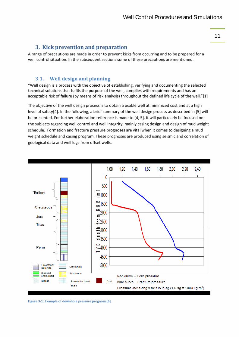
3.1. Well design and planning“Well design is a process with the objective of establishing, verifying and documenting the selectedtechnical solutions that fulfils the purpose of the well, complies with requirements and has anacceptable risk of failure (by means of risk analysis) throughout the defined life cycle of the well.”[1]
The objective of the well design process is to obtain a usable well at minimized cost and at a highlevel of safety[4]. In the following, a brief summary of the well design process as described in [5] willbe presented. For further elaboration reference is made to [4, 5]. It will particularly be focused onthe subjects regarding well control and well integrity, mainly casing design and design of mud weightschedule. Formation and fracture pressure prognoses are vital when it comes to designing a mudweight schedule and casing program. These prognoses are produced using seismic and correlation ofgeological data and well logs from offset wells.
Figure 3-1: Example of downhole pressure prognosis[6].

Well Control Procedures and Simulations12In the figure a fictive pressure prognosis is shown. However, these pressure profiles are typical. This
may be used as an illustration for the sections to come.
3.1.1. Mud weight scheduleThe optimal mud weight for the various hole sections is determined as a compromise between arange of different considerations. Although most literature suggests using a mud weight close to theformation pressure in order to increase the drilling rates, [5] recommends using a relatively high mudweight. Use of a median line principle when designing a mud weight program is suggested. Themedian line is obtained as the arithmetic average of the pore pressure and the fracture pressure.This is said to have positive effect with regards to a range of borehole problems. A summary of theprinciple is given as follows:
“
1. Establish a pore pressure gradient curve and a fracturing gradient curve for the well. Thefracture gradient curve should be corrected for known effects like wellbore inclination andtectonic stresses.
2. Draw the median line between the pore and the fracture gradient curve.3. Design the mud weight gradient to start below the median line immediately below the
previous casing shoe.4. Mark out depth intervals prone to lost circulation and differential sticking, and their
acceptable mud weight limits, if known.5. Design a stepwise mud weight schedule around the median line that also takes into account
limitations from 3 and 4 above.6. Avoid reducing the mud weight with depth. If a median line reversal occur, keep the mud
weight constant.” [5]
Safety margins as trip- and riser margins should be included when determining the correct mudweight. There should also be a margin towards the fracture pressure. Often the safety margins areset to a minimum of 2 points SG. Thus, the mud density should lie between the equivalent mudweight of the formation added a safety margin of 0,02 SG and equivalent mud weight fracturepressure subtracted a safety margin of 0,02 SG. If the median line principle is used, these safetymargins are often already included in the mud weight schedule.
3.1.2. Casing designCasing design and setting depth relies on a range of different factors and considerations. In thissection however, only considerations related to burst will be presented, as this is most importantwith respect to well control.
The ordinary casing dimensions used at the NCS is as follows:
30 inch conductor 20 inch surface casing 13 3/8 inch intermediate casing 9 5/8 inch production casing 7 or 5 inch liner
When designing a casing program load cases have to be defined. The casing strings have to withstandthe loads which they might be exposed to during the life cycle of the well. The scenarios in which themaximum loads are expected are called worst case scenarios. When it comes to burst failure, theworst case scenarios are often defined as

Well Control Procedures and Simulations13 Gas filled wellbore, or
Predefined kick tolerance requirements
Kick tolerance is defined as the maximal influx size which can be circulated out of the wellborewithout fracturing at the shoe. The maximum pressure induced at the casing shoe may be calculatedanalytically by estimating an influx density or determined by simulations. This again has to becompared with the fracture pressure at the casing shoe, obtained by the fracture pressure prognosis.Generally, the calculated maximum pressures are more conservative than the simulated. ModernWell Design[5] offers a kick tolerance guideline for floating drilling units. It suggests a kick toleranceof 1-8 m3. This is based on the accuracy of the surface volume measurements in the active fluidsystem wellsite.
Using the gas filled wellbore scenario as a design criterion, the well is said to have full well integrity.Both the casing string and the open hole section can withstand the pressures exerted by a gas filledwell. From a well control point of view, this is highly beneficial. However, this concept may result in adisadvantageous amount of casing sections. This is problematic with respect to time, cost anddownhole and topside clearances (geometrical problem).
If the kick tolerance concept is used, the well is said to have reduced well integrity. Thus, the well canonly handle a certain influx volume without losing its integrity. What is vital when applying thisscenario as a design criterion, is that the weakpoint of the well is located in the open hole section ofthe well. This means that if a kick of higher intensity than the predefined kick tolerance is taken, thewell will fracture in the open hole section, rather than bursting the casing.
Using the predefined load cases, the required load ratings of the casing sections can be calculated.This is done by introducing a design factor or a safety factor. The minimum design factors to beapplied in casing design can be found in the table below.
Burst Collapse Tension Tri-axialMinimum design factors 1,1 1,0 1,3 1,25Table 3-1: Minimum design factors for casing design purposes[1].
The approach using minimum design factors in casing program design is often referred to asdeterministic. It is required that the pressure rating of the casing fulfills the relation:
(3.1)
The casing load rating is supplied by the manufacturer. In general, the casing joints are made incorrespondence with [7], and the ratings are tabulated in for instance [8]. For bottomholetemperatures higher than 100 ˚C[5], a down rating of the casing is necessary. This has to be donewith reference to the manufacturer of the casing.
As a substitute for the deterministic approach, also probabilistic calculations may be used. In thiscase, the probability of failure should not exceed 10-3,5 [1]. A further description of the probabilisticapproach is to be found in[4].
Generally, the production casing is set just before drilling into the reservoir zone. The productioncasing will have to provide full well integrity. Thus, both the casing and the open hole formationneeds to withstand the pressures caused by the gas filled well scenario. Sometimes the productioncasing is design to match the pressure rating of the wellhead and BOP equipment.

Well Control Procedures and Simulations14For production and drill stem testing also a third scenario has to be considered. Leaking tubing
immediately below the well head will subject the completion fluid in the annulus between the tubingand production casing (or tie-back) to the flowing pressures inside the tubing. The completion fluidwill in general be more dens than the produced fluids. This will cause a collapse pressure on thetubing and a burst pressure on the non-cemented sections of the production casing.
For the intermediate casing sections, a reduced well integrity may be sufficient. Thus, if the worstcase scenario should occur, the formation will fracture rather than the intermediate casing. This willcause an underground blow-out, but this may in some cases be regarded acceptable. For thesesections the concept of kick tolerance is introduced.
The conductor and the surface casing have very limited well control applications. Their main functionis to provide a proper fundament for the wellhead, BOP and the subsequent casing sections. Still, it isassumed that the surface casing should be subject to integrity calculations.
Casing setting depth is limited by formation pressure and fracture pressure, and the planned mudweight schedule. The setting depth of each string is determined by starting at the bottom of the welland moving upwards. In this way, the amount of casing sections can be reduced to a minimum. Everycasing seat should be located in a competent and impermeable formation. This should be done inorder to provide structural strength and to avoid fluid migration in the vicinity of the casing seat.
3.1.3. Well design exampleThis can be the results of a preliminary casing and mud weight program. At this point, calculations onwell integrity have not yet been performed. Neither, will they be, as this section merely intends toserve as an example. The premises for this preliminary plan will be briefly outlined in the following.
Figure 3-2: Preliminary mud weight schedule and casing program. The scale on the abscissa is in specific gravity and thepressures are measured in mud weight equivalents. The red and blue lines represent the formation pressure and the

Well Control Procedures and Simulations15fracture pressure with dotted safety margins. The solid black line is the mud weight schedule, while the dotted black line
is the maximum hydrostatic pressure exerted at the open hole section.
The dotted lines in the vicinity of the fracture pressure and the pore pressure are safety margins. Inthis case they are set to 0,02 SG. The black dotted line is the maximum hydrostatic pressure exertedby the drilling fluid on the open hole sections. The scale on the abscissa is specific gravity, and thepressures are measured in equivalent mud weight.
It can be seen that a sand zone is situated below a stringer of coal at around 1000 m RKB (Figure 3-1).The coal may function as a sealing structure for the sand zone. Therefore, shallow gas may beexpected. Depending on seismic and data from offset wells, it should therefore be evaluated to drill apilot hole prior to drilling the top hole. If shallow gas is present, further drilling at this location shouldbe re-evaluated according to a shallow gas contingency plan.
For drilling the top hole, sea water and high viscosity pills are used. The conductor is set 100 m belowseabed. The seat of the surface casing is situated at 1425 m RKB. This is at the bottom of acompetent shale formation (Figure 3-1). After setting and cementing the surface casing, the BOP andriser is run, and returns are taken back to the rig.
For the intermediate section the mud is weighed up twice. The first 200 m of the intermediatesection is drilled using a mud weight of 1,23 SG. At 1625 m RKB the mud is weighed up to 1,59 SG.This is done with reference to the median line principle. It is possible to place the intermediate casingshoe as deep as 3500 m RKB with respect to the suggested mud weight. This will however cause themud weight to approach the formation pressure, which could again cause borehole problems.Therefore it was decided to place the casing shoe at 2850 m RKB. This is the shallowest setting depthpossible while still remaining in overbalance in the reservoir section.
The first 200 m of the production section is drilled with the same mud weight as the final interval ofthe intermediate section. Then the mud is weighed up to 1,78 SG. 250 m before the seat of theproduction casing, the mud is again weighed up to 1,87 SG. The production casing is set at 4250 mRKB in a competent chert formation (Figure 3-1).
Drilling into the reservoir, the mud weight is kept constant at 1,87 SG. This is in slight contradictionwith the median line principle. However, it is believed that it is important to use a low density fluid asa drill-in fluid in order not to cause formation damage in the reservoir. This is of particularimportance if a drill stem test is to be conducted, or if the well will be used for production purposes.
The simulations of section 9.2 will to some extent be based on the outlined program describedabove.
3.2. Preventive operational procedures“Loss of primary well control is usually due to:
Failure to keep the hole full.
Swabbing.
Insufficient drilling fluid density.
Lost circulation.”[2]
From spudding until the well is permanently plugged and abandoned, the objective of the preventivewell control procedures is to avoid these situations to occur. Thereby, a well control situation may beprevented.

Well Control Procedures and Simulations16Where nothing else is stated, the procedures presented in these sections are as outlined by a major
drilling contractor[3].
3.2.1. TrippingTripping refers to pulling a string out of hole or running a string in hole. The majority of all kicks aretaken while tripping out[3]. Therefore it is important to have good procedures in order to preventthis from occurring.
Failure to keep the hole fullFailure to keep the hole full is a problem associated with tripping out of hole. As pipe is pulled fromthe hole, the volume previously occupied by the pipe will have to be replaced with mud. This isachieved by continuously circulating on the trip tank. The trip tank has to be refilled as the fluid levelin the tank drops. A trip sheet is applied in order to verify that the hole is taking the correct amountof mud, and to identify any overall losses or gains in the total active fluid system.
The pipe should preferably be pulled dry, in order to improve volume control. This is achieved bypumping a slug of high density mud. Should this for any reason be impossible, a mud bucket could beapplied.
“If the hole does not take the correct volume of mud, or if the Driller has any doubt, the pipe must berun immediately and cautiously back to bottom and bottoms-up circulated.”[3]
When tripping in hole the drillstring is filled with mud at regular intervals. It is important that afailure in the float valve and subsequent u-tubing of mud into the drillstring, should not cause thehydrostatic pressure exerted bottomhole to fall short of the formation pressure. Calculations shouldbe performed, when deciding upon the intervals between filling the drillstring.
SwabbingSwabbing is a problem associated with tripping out. For small clearances between the BHA and theborehole walls a piston like effect can be produced. The actual pressure loss due to swabbingdepends on the pulling speed, the properties of the formation and the drilling fluid and on thegeometrical clearances present downhole. The effect can be intensified due to bit-balling and pack-off, a thick filter cake or extensive heave. If the swabbing causes the well to go underbalance, theresult can be trip gas or a swabbed kick.
The trip margin should be calculated before pulling out of hole. It is calculated as the differencebetween the mud weight and the equivalent mud weight corresponding to the formation pressure.The trip margin is an expression for the static overbalance in the well.
The trip velocity should be limited. Permissible pulling speeds can be determined by computersimulations. If the simulation software is not available wellsite or at low trip margins it should beevaluated to perform a short trip. The short trip is executed at the determined pulling speed.Typically 5-10 stands are pulled, before running back to bottom, flow checking and circulatingbottoms up. The measured percentage of gas in the returns will show if the determined pulling speedis suitable.

Well Control Procedures and Simulations17If there is a risk of swabbing a kick, pumping out of the hole should be considered[3]. This will
continuously replace the volumes previously occupied by the drillstring with mud. In addition, thiswill expose the well to a frictional pressure gradient, which assists in maintaining overbalancetowards the formation.
Lost circulationAs pipe is run in hole a pressure surge may develop in front of the BHA. This effect is similar toswabbing, and can cause mud loss to the formation or even fracturing.
As for pulling out of hole, tripping velocities should be limited. This is of particular importance in theopen hole sections. Permissible running speeds can be obtained by computer simulations.
It should be evaluated to break circulation before entering the open hole section. This can functionas a means for reducing the pressure surges.
“Any time a trip is interrupted the hand tight installation of a safety valve is required.”[3]
3.2.2. DrillingAlthough it is established that the most kicks occur during tripping, a reasonable amount of kicks aretaken during drilling.
Failure to keep the hole fullDuring drilling there is a constant circulation of drilling fluid. This generally ensures that the well iskept full at all times. However, the volumes in the active pits should be continuously monitored. Achange in the active surface volume could indicate either a flowing well or lost circulation.
SwabbingSwabbing is generally not an issue during drilling. This is due to the fact that the bit and BHA issituated at the very bottom of the well, with very limited axial movement. However, if a drilling standis used, swabbing may occur when pulling the drilling stand for a connection. It is assumed that aslong as the drilling stand is pulled with the mud pumps running, the risk of swabbing a kick will beinsignificant.
Insufficient drilling fluid densityThe mud should be treated and conditioned in order to have the density given by the drillingprogram. Density and other mud properties should be measured both in and out of the holeregularly. The mud conditioning equipment should be maintained and adjusted to work optimalunder the conditions encountered.
Excessive drilling rates should be avoided in the presence of background gas and water bearingformations. This is important as cut mud will have a reduced density. The gas fraction is to becontinuously monitored by mud logging engineers.
When drilling with a marginal overbalance, it is important to be aware of the drop in downholepressures as the pumps are shut down for connection. A well could be in slight overbalance whilecirculating, but as soon as the pumps are shut down the well might go in underbalance. If asubsequent gas influx is taken, this is called connection gas, and will reduce the hydrostatic pressureof the fluid column.
Well Control Procedures and Simulations18Lost circulation
Circulation loss may be caused by leaks to permeable formations or natural fissures in the open holesection. It can also be caused by inducing formation fractures due to a high overbalance. In general,small seepage losses are to be expected until the mud has built a filter cake on the borehole walls.
It is important to be aware of the friction loss in the annulus and riser. The downhole pressures arehigher during circulation than at static conditions. It is of particular importance to take care whenbreaking circulation. Drilling fluids are often non-Newtonian, and static mud may require a relativelyhigh yield pressure in order to break the gel. It is therefore good practice to start rotating thedrillstring before breaking circulation. This way, the gel will be broken in a gentler manner.
3.3. Procedures for well control preparednessIn order to being able to conduct the proper calculations prior to a kill procedure, information aboutthe fracture pressure and dynamic pressure loss in the circulating system has to be known. This isregularly measured wellsite in form of leak-off tests and SCRs. A brief presentation of theseprocedures is included in the following sections.
3.3.1. Leak-off testLeak-off tests are used to measure the fracture pressure of the leak-off pressure of the formation. Aleak-off test is generally conducted after drilling out a casing shoe and a few meters of newformation. Additional tests can also be conducted further down in the open hole section, ifformations expected to have a lower fracture gradient are encountered. The obtained leak-off valuesare used as estimations of the fracture pressures of the open hole section. If a measured leak-offvalue is lower than suggested by the fracture pressure prognosis, this will affect the kick tolerance ofthe section to be drilled.
The obtained leak-off pressure is used for calculating maximum allowable annular surface pressure(MAASP), which has its application in the initial phase of circulating out a kick.
3.3.2. Slow circulating rateThe dynamic pressure loss in the wellbore system is measured well site on a regular basis. Thesemeasurements are done while circulating with a constant and slow circulation rate (SCR). The rate ofcirculation is corresponding to a small range of possible predetermined kill rates (2-3 arerecommended by [2]). Typical pump output rates are 20-50 spm, corresponding to the short side of400-1000 lpm. The drillpipe pressure is recorded during normal circulation, and during circulationthrough the chokeline.
The SCR is measured at regular depth intervals. It is also measured after changing out BHA or bitnozzles, at altered mud properties (density, viscosity), after major repairs or modifications on thehigh pressure circulation system, etc.
The SCR measurements are used extensively in the calculation preceding a well kill.

Well Control Procedures and Simulations19
4. Kick detectionIt is vital to monitor the well continuously in order to be able to act efficiently upon taking a kick. Theresponse time after a kick is taken, determines the size of the influx, and thereby the severity of thewell control situation.
4.1. Kick indicatorsThere exists a variety of parameters which may indicate a kick. A selection of these is presented inthe following sections.
“Establish baseline reading and continually monitor for any variation in trends for gas, mud, cuttingsand drilling parameters.”[3]
4.1.1. Increase in return rate and surface volumesThe most direct indicators of a kick are an increase in returns relative to the pump rate andsubsequently, a gain in the surface active fluid system. This is caused by influx fluids displacing thedrilling fluids downhole. It is important to have sensitive volume gauges for measuring the activesurface volume.
“Consider fingerprinting the flowback trend having shut off the pumps for a connection. Establish abaseline and closely monitor for any variation in this trend during subsequent connections.”[3]
4.1.2. Increase in drillabilityWhen drilling into an abnormally pressured formation, the overbalance (chip hold down pressure[9])will be reduced. This may result in an increase in penetration rate. If the increase is significant (100%or more over 5 ft drilled formation[3]) this is called a drilling break. However, the penetration rate isadditionally a function of a range of other variable drilling parameters. Therefore the concept ofdrillability is introduced. The drillability is a more or less empirical function of the relevant drillingparameters and intends to give a qualitative value of the formation pressure and drilling resistance.Thus, the drillability is independent of the drilling parameters.
The d-exponent
(4.1)[10]
Where drillability, d-exponent
Rate of penetration
Weight on bit
Rotational velocity (typically RPM)
Bit diameter
Well Control Procedures and Simulations20An increase in drillability is not necessarily due to drilling into a potentially kicking formation. Similar
effects would also be present when simply drilling into a softer formation. However, all drillingbreaks must be flow checked[3].
4.1.3. Other drilling parametersWhen drilling into an abnormally pressured zone an increase in torque is expected. This is due to thechip hold down effect. When the dynamic bottomhole pressure approaches the formation pressure,the cuttings in front of the drill bit will be pushed away. This may further cause a high concentrationof cuttings around the BHA, which will in turn increase the torque.
Upon taking a kick, a decrease in drillpipe pressure might occur. As the lighter kick fluids enter theannulus, the u-tube effect will cause lower pressures throughout the internal length of the drillstring.
4.1.4. Drilling fluid propertiesThe drilling fluid properties will change according to its composition (gas/water cut). The drillingfluids will generally contain a concentration of formation fluids. This comes from diffusion from thedrilled formation and the cuttings. If the dynamic bottomhole pressure approaches the formationpressure, there will be an increase in net diffusion. This will give a decrease in density and a changein viscosity. The change in viscosity depends on the chemical properties of the mud emulsion/invertemulsion and its compatibility with the formation fluid. This is not seen before the mud is circulatedto surface, and it is in that sense a delayed indicator.
4.1.5. Cuttings geometryThe cuttings geometry might change when encountering an abnormally pressured formation. This isdue to the chip hold down effect, and will result in larger and more angular cuttings. This is also adelayed indicator, as a bottoms-up circulation is necessary in order to observe the cuttings geometrytopside.
4.1.6. Increase in background gasWhen drilling in a gas bearing formation, the return mud will generally have a small and relativelystable gas concentration. This is called background gas, and is due to diffusion from the cuttings andthe formation. If the dynamic bottomhole pressure approaches the formation pressure, there will bean increase in background gas. Spikes in the background gas might also be observed afterconnections. This is called connection gas, and is caused by a further decrease in bottomholepressure when the pumps are shut off.
4.1.7. Increase in temperatureShale often functions as a seal for high pressured formations. The thermal conductivity of shale isrelatively low. Hence, heat will accumulate in the formation below the shale. When drilling into anabnormally pressured formation, an increase in drilling fluid temperature may be seen topside. Thiseffect can function as a delayed kick indicator.

Well Control Procedures and Simulations21
4.1.8. Downhole measurementsThe bottomhole assemblies of today are composed from various sophisticated tools for logging andmeasuring formation and borehole data while drilling. A change in the rock and fluid properties ofthe formation would easily be detected. However, the MWD/LWD tools are only functional in thelateral direction. Their position behind the bit will cause a delay of several meters.
4.2. Flow check“A flow check must be conducted any time the driller has doubt about the stability of the well.”[3]
If any kick indications should occur, the well will be flow checked. This is done by shutting down themud pumps and lining the returns through the trip tank. From the trip tank, mud is pumped backthrough a fill up line into the top of the riser. If the well is stable, the mud level in the trip tank willremain constant. Increase in trip tank volume while flow checking will further indicate a flowing well.A typical flow check lasts for 10-15 minutes.
The reasons for lining up the mud flow through the trip tank, is that the accuracy of the volumemeasurements are higher than for the mud pits. This is due to a smaller cross sectional area of thetrip tank, so that a small increase in volume will result in a relatively high increase in liquid height inthe trip tank.
There are several effects to be aware of when flow checking. A gain in the trip tank immediately aftercommencing a flow check is not uncommon, even if the well is not flowing. These gains can be aslarge as 100-200 bbls or 16-32 m3 [5], and can easily be misinterpreted as a kick. The flow trendswhile flow checking should therefore be monitored and compared in order to distinguish an actualkick from the false indications. However, “if there is any indication of flow consider shutting in thewell immediately rather than taking the additional time to conduct a flow check”[3].
This type of wellbore backflow is called ballooning. Ballooning is actually caused by a range ofdifferent effects:
Expansion of the mud due to downhole heat conduction from the formation will cause aninflux indicator.
A reduction in pressure gradient throughout the well when the mud pumps are shut off willcause a slight pressure expansion of the mud. The same mechanism might also cause a fluidexchange with the formation, where both intruded mud and formation fluid will enter thewellbore. If the formation fluid is light, this will further cause a delayed increase in thebackground gas reading, similar to connection gas.
It is also a general belief that the borehole walls are elastic, and that a reduction in downholepressure gradient will cause a wellbore contraction. This will yield a further gain in the triptank. Simulations have shown that this effect contributes 5-14%of the net gain caused bypressure effects[5].
Well Control Procedures and Simulations22
5. Influx containmentAfter taking a kick, the influx should be shut-in as soon as possible. This is managed by closing theBOP preventers and the valves on the kill- and chokelines. The situation after shutting in the well isnormally:
Drillstring hung off at pipe ram Annular preventer closed Failsafe valve on kill line closed Failsafe valve on chokeline open Choke valve closed
After the well is stabilized, the shut-in pressures can be read. SICP is read below the choke valve andSIDPP is read at the standpipe manifold. Both SICP and SIDP are important parameters when it comesto the design of a kill program.
API RP 59[2] differentiates between hard and soft shut-in.
5.1. Hard shut-inDuring normal drilling operations the BOP preventers are open and the failsafe closed. All valves onthe chokeline are open and lined up towards the poor boy separator with exception of the remotechoke valve and the valve immediately upstream or downstream of the choke. If a kick is taken, theshut-in procedures are as follows[2, 3]:
Pull bit off bottom Space out Shut down mud pumps Stop drillstring rotation Close annular preventer and open the chokeline failsafe valves Close pipe ram below tool joint, and hang off drillstring Inform toolpusher and operator representative Determine SICP and SIDPP
5.2. Soft shut-inIf soft shut-in is the desired containment procedure, the failsafe valve on the chokeline is closedduring normal operations, while the choke valve is open. The other chokeline valves are open andlined up to the poor boy degasser. The valves on the kill line are all closed and the BOP preventersare open. If a kick is taken, the shut-in procedure is as follows:
Pull bit off bottom Space out Shut down mud pumps Stop drillstring rotation Close annular preventer and open the chokeline failsafe valves Open failsafe valve on chokeline Close choke gradually

Well Control Procedures and Simulations23 Close pipe ram below tool joint, and hang off drillstring
Inform toolpusher and operator representative Determine SICP and SIDPP
This procedure is partially based on the information found in [2].
6. Removal of influx fluid from the wellboreIf a kick is taken and the well is shut in, an appropriate kill procedure is to be initiated. Killing a wellrefers to removal of influx fluids from the wellbore, and re-establishment of the mud column as theprimary barrier. NORSOK[11] lists four possible kill methods:
Driller’s Method Wait & Weight Volumetric Method Bullheading
The first two methods are widely used, while the two latter are only used in special situations. Anintroduction to the four kill methods will be presented in the subsequent sections.
When killing a well by conventional methods, kill sheets are applied. The kill sheets ease thecalculation and design of a well kill operation, and should be systematically updated[1]. Examples ofstandard kill sheets are included in the appendix.
6.1. Driller’s methodDriller's method is a simple method for circulating out a kick. The method is applicable if the bit is onbottom. If not, stripping to bottom will be necessary. The kill procedure is completed in two roundsof circulation. The kick is circulated out in the first round of circulation. This is done using the olddrilling fluid. In the second round of circulation, the well is displaced to kill mud, and the primary wellbarrier is re-established. During the whole process, it is important to keep the dynamic bottomholepressure constant and slightly higher than the formation pressure. This is to avoid further influx offormation fluids. The pressure at the weakpoint should also be lower than the fracture pressure, inorder to avoid an underground blowout.
The kick is circulated out in the first round of circulation, using the old mud. The mud pump isgradually brought up to a predetermined slow rate. This is done while adjusting the choke valve. Onsubsea wells a constant BHP may be achieved by keeping the kill line pressure constant, whilebringing the pump up to speed (annular pressure loss is assumed negligible)[2]. When the pump isrunning at kill rate, the drillpipe pressure will be held constant at the initial circulating pressure (ICP)throughout the first round of circulation. This is achieved by applying and adjusting the backpressureon the choke valve. As the drillstring is assumed to contain homogeneous mud of known density, thebottomhole pressure will be constant as long as the drillpipe pressure kept constant.
The ICP is defined as:
The equation is defined and deduced in section 7.

Well Control Procedures and Simulations24If the first round of circulation is a success, the influx will be completely removed from the wellbore.
This can be checked by shutting down the pump and closing in the well synchronously, while stillkeeping constant bottomhole pressure. Thus, the drillpipe pressure will have to be reduced by thedynamic pressure loss measured through the riser. If the entire influx is removed, the static pressureson both the drill pipe side and the casing side should be stable and equal.
The second round of circulation is performed using drilling fluid at kill mud density. This is done inorder to re-establish primary well control. The kill mud weight is calculated in the kill sheet, and is setto balance the formation pressure with a slight overbalance (safety margin). The pump is broughtgradually up to kill rate at constant kill line pressure by adjusting the choke backpressure. Casingpressure is kept constant until the kill mud reaches the bit. While the kill mud is pumped up theannulus, drillpipe pressure should be kept constant at final circulating pressure (FCP). After the entirewell is displaced to kill mud, the shut-in pressures should be reduced to the atmospheric pressure.
The equation is defined and deduced in section 7.
Driller's method is perhaps the most used method for circulating out a kick. The method has severaladvantages. Upon shutting in on a kick, the circulation may commence immediately, withoutweighing up to kill mud. This is important if the influx fluid is compressible gas in water based mud,as gas migration may cause high pressures in the wellbore. Driller's method is also quite easy for thechoke operator. The choke can be adjusted to maintain constant drillpipe pressure until the kick isout of the system.
In section 9 a couple of calculation examples on driller’s method are included. In section 10simulations on driller’s method are conducted. The results of calculations and simulations will befurther discussed and compared in section 11.
6.2. Wait & weightThe wait & weight method is very similar to driller's method. Wait & weight also uses circulation as ameans for removing the influx and restoring the primary well barrier. And as for driller's method, aconstant bottomhole pressure is key. The difference is that circulation with kill mud startsimmediately. This means that the kick is removed and the well displaced to kill mud in one singleround of circulation.
The pump is brought slowly up to kill rate while adjusting the choke, so that the kill line pressure iskept constant. At kill rate, the drillpipe pressure should be approximately equal to the calculatedinitial circulating pressure (ICP). If not, the reason should be investigated. As circulation proceeds, thedrillpipe pressure should be reduced linearly as calculated in the kill sheet. When the wholedrillstring is displaced to kill mud, the drillpipe pressure has reached the calculated final circulatingpressure (FCP). For the rest of the circulation, the drillpipe pressure should remain constant at finalcirculating pressure.

Well Control Procedures and Simulations256.3. Static volumetric method
The static volumetric method can be used if circulation through the drillstring for some reason isimpossible. It also finds its application in combination with the above mentioned kill methods. Inparticular when gas migration is causing excessive pressure build up before the desired kill method isinitiated.
The intention of the method is to keep the bottomhole pressure constant (including a safety margin)while the kick migrates up the annulus. This is achieved by stepwise bleeding off mud through thechokeline, while controlling choke backpressure. With drillstring communication (possibility tomeasure drillpipe pressure) volumetric method is conducted with ease. As mud is being bled off, thechoke backpressure is adjusted with reference to the drillpipe pressure. Mud should be bled off untilthe drillpipe pressure reaches the prerecorded shut-in pressure added a safety margin (typically 100psi[2]). This ensures that the bottomhole pressure remains within a predetermined interval, and nofurther influx will occur.
With loss of drillstring communication, use of the static volumetric method becomes morecomplicated. This will not be presented here.
6.4. BullheadingBullheading is a method where the influx is pumped back into the formation without returns tosurface, using a constant pump rate. During the pumping the injection pressure should be lowenough not to fracture the formation at the weakpoint. Exceeding the fracture pressure may provokean underground blowout, instead of killing the well.
Bullheading is used when H2S is expected to be present amongst the influx fluids, or when the margintowards the fracture pressure is to low for a conventional kill to be performed (driller’s method orwait & weight). The method can also be used when the drillstring is out of hole, as kill mud can bepumped through the kill- and chokelines. Bullheading is most successful when the open hole sectionis relatively short[2].

Well Control Procedures and Simulations26
7. An analytical modelIn order to derive the traditional well control formulas, a series of simplifying assumptions has to bemade. This set of assumptions to derive a simple analytical model. This model finds its application inmost practical well control operations at wellsite.
7.1. Assumptions Conservation of mass Constant pressure gradient in the drilling fluid (non-compressible) Gas influx acts according to Boyle's law Influx propagates as a single bubble No temperature gradient Negligible frictional pressure loss in annulus and riser Chokeline friction and drillstring friction directly proportional to the fluid density No phase transitions between influx and drilling fluid Constant wellbore volume (No fluid exchange with the formation, inelastic formation) Simplified wellbore geometry
This will be further elaborated in the sections to come.
7.1.1. Conservation of massConservation of mass is valid for the entire system. For any timestep or displacement in position, theincrease or decrease in accumulated mass in a control volume, is equal to the mass which has flowedinto the control volume subtracted the mass which has flowed out.
(7.1)
The well is treated as a constant volume (inelastic wellbore and casing) with an inlet at the drillstringside and outlet at the annulus side. This volume may function as a control volume. It is assumed thatno fluid is lost to the formation. With exception of a kick situation, the inflow rate from the formationis also assumed to be zero at all times. The latter assumption is generally valid, due to a hydrostaticoverbalance in the wellbore.
7.1.2. Fluid propertiesIn general, the density of the drilling fluid is a function of temperature and pressure. However, thedrilling fluid is approximated to be incompressible. This means all changes in density due totemperature and pressure are neglected. An implication of this assumption is that the speed ofsound in the liquid phase in infinite. Any changes in pressure in one point in the liquid column, isinstantaneously measured throughout the entire volume of liquid. Since the density is assumedindependent of pressure, the mass conservation also implies conservation of liquid volume.

Well Control Procedures and Simulations27The influx gas is treated as a single bubble propagating with no-slip or constant slip through the
drilling fluid. No phase transitions are assumed between the liquid phase and the gas phase. Thisassumption is quite accurate using water based drilling fluids. However, for oil based mud, methaneand other light hydrocarbon gases may go in complete solution with the drilling fluid. As thedissolved gas is circulated to surface, the pressure is gradually reduced. When the pressure crossesthe bubble point, the dissolved gas may suddenly boil out of solution.
In general gas behaves according to the real gas law.
(7.2)[12]
Where Absolute pressure in the gas
Gas volume
Absolute temperature in the gas
Compressibility factor of gas
Number of gas molecules in the gas volume
Gas constant, 8.31 J·K−1·mol−1
The compressibility factor is depending on the type of gas, and the temperature and pressure. Forideal gas or at atmospheric pressure and temperature the factor equals one. The temperaturegradient in the well will depend on the dynamic conditions in the well. At static or steady stateconditions the temperature gradient in the wellbore fluids will reach equilibrium with thetemperature gradient in the formation (neglecting convection). However, this equilibrium will bedisturbed by changing the rate of circulation. Both compressibility and temperature can be modeledby more or less empirical approximations.
In most of the traditional well control formulas the temperature dependency of the ideal gas law isneglected. Further, the compressibility factor z, is assumed to equal one. Thus, the gas is assumed tobehave according to Boyle’s Law.
(7.3)
Where Absolute pressure in the gas
Gas volume
7.1.3. Pressure balanceThe pressure balance during dynamic conditions can be expressed as

Well Control Procedures and Simulations28
(7.4a)
(7.4b)
Where Bottomhole pressure
Choke pressure
Hydrostatic pressure exerted by the fluids
Frictional pressure loss in the annulus
Frictional pressure loss in the chokeline or riser
Frictional pressure loss in the drillstring
Pressure loss across the bit
The first equation expresses the pressures on the annulus side, and the second on the drillstring side.At static conditions, the frictional pressure loss and the pressure loss across the bit will equal to zero,and the equations will be reduced to the following
(7.5a)
(7.5b)
This result is of particular importance, and will be applied extensively in the sections to come.
7.1.4. Drillpipe and casing pressureThe drillpipe- and the casing pressures are measured at drill floor level. At static conditions, with noshut-in pressures, these will be equal to the atmospheric pressure. During pumping, the drillpipepressure will in general reflect the flow resistance in the wellbore system, as the hydrostatic pressurein the drillstring and annulus are close to equal. In a kill situation, the circulation will take placethrough the chokeline. In this case, the casing pressure may be manipulated by choking the flow atthe choke manifold.
7.1.5. Hydrostatic pressureThe hydrostatic pressure is the pressure exerted by the weight of a static fluid column. A standardform for expressing this is

Well Control Procedures and Simulations29(7.6)[12]
Where Difference in hydrostatic pressure between two points of interest
The fluid density between the two points of interest
The acceleration of gravity
The vertical distance between the two points of interest
This might seem straight forward. However, in reality, the fluid density is a function of thetemperature and the pressure. The pressure is again depending on time and position. Due to fluidcompressibility, the hydrostatic pressure gradient will increase at increasing pressures and vice versa.In the derivation of the traditional well control formulas, these effects are neglected. Thus, the liquidcompressibility is set to zero. For conventional drilling the mud weight is set to provide a slightoverbalance to the formation pressure.
7.1.6. FrictionFluid friction works in the opposite direction of the flow. It is actually the resistance of flow betweeninfinitesimal layers of fluid moving at different velocities. Fluid friction for flow in a pipe with circularcross section can, in general, be expressed as (Ref Drilling Engineering)
(7.7)
Where Friction factor
Fluid velocity
Inner diameter of the pipe
The distance along the flowpath between the two points of interest
The other symbols are defined in the previous sections.
The friction factor may be found as various functions of the Reynolds number, depending on the flowregime. The Reynolds number is defined as
(7.8)[12]
Where Fluid viscosity

Well Control Procedures and Simulations30
For low Re, typically less than 3000 using SI units, the flow is considered laminar. For higher Re, theflow is turbulent. Laminar flow typically occurs in the annulus and riser. It can be shown that thefriction factor for laminar flow equals
(7.9)[12]
The flow inside the drillstring and through the chokeline is normally turbulent. For turbulent flow,only empirical correlations for the friction factor exist, usually proportional to the Reynolds numberto a small negative power. In the analytical model, this dependency is neglected, so that
(7.10)
The dynamic pressure loss (SCR) in the wellbore system is measured well site on a regular basis. Thedrillpipe pressure is recorded during normal circulation, and during circulation through the chokeline.By setting the drillstring side and the annulus side of the pressure balance equal to one another, thebottomhole pressure cancel out. Further, assuming no compressibility, the hydrostatic terms cancelone another. Solving the pressure balance with respect to the difference between drillpipe pressureand casing pressure yields
(7.11)
Where Dynamic pressure loss at kill rate
The frictional pressure terms in the annulus and riser are normally small compared to the otherterms. Often, these pressure losses are neglected completely. Assuming a riser friction loss of zeromakes it possible to calculate the frictional pressure loss in the chokeline. Simply by subtracting thedynamic pressure loss through the riser from the dynamic pressure loss through the chokeline, onewill obtain
(7.12)
These results will be made further use of in the sections to come.
Well Control Procedures and Simulations31
7.1.7. Pressure drop across bit and choke valveThe following derivation is made with reference to[5]. The pressure drop across the bit and chokecan be modeled as an abrupt reduction in cross section, assuming incompressible and inviscid flowalong a streamline. Under these conditions Bernoulli’s theorem is valid. The theorem states that
(7.13)[12]
Where Vertical position
The pressure drop across the cross sectional reduction is obtained by further assuming the kineticenergy before the flow obstruction to be negligible. The vertical displacement is assumed to be zero.By replacing the fluid velocity at the point of obstruction with the volumetric flow rate divided by thecross section one obtains
(7.14)[5]
Where Volumetric flow rate
Total flow area through the bit nozzles or the choke opening
Discharge coefficient
The discharge coefficient is added in order to match the theoretical equation with experimentalresults. The value of the coefficient depends on the design of the choke valve or the bit nozzles. Atypical value for the bit is 0,95 (dimensionless).
7.2. Derivation of some of the traditional well control formulasThe above mentioned relations and assumptions, result in a simple analytical model. This model maybe used in the deduction of some of the traditional well control formulas. The validity of some of theassumptions, and the errors produced by the following well control formulas, will be investigated inthe discussions sections.
Upon taking a kick and shutting in the well the following data are known or can be measured.
SIDPP and SICP Pit gain Dynamic pressure loss at kill rate LOT data

Well Control Procedures and Simulations32 Wellbore geometry and drill floor elevation
Drilling fluid density at standard conditions
The derived formulas will have to be functions of these parameters.
7.2.1. Standard kill formulasIn order to obtain a value for the formation pressure upon taking a kick, it is assumed that thebottomhole pressure exactly equals the pressure of the formation. By using equation (7.5b) and (7.6)with an assumption of incompressible mud in the entire drillstring, one obtains
(7.15)[8]
Where Formation pressure
Drillpipe pressure at shut-in
Density of current drilling fluid at standard conditions
True vertical well depth
The kill mud is designed to exactly balance the formation pressure, so that the drillpipe pressure isreduced to the atmospheric pressure when the kill mud reaches the bit. Thus,
(7.16)
Where Kill mud density at standard conditions
Or, by making use of the right hand sides of equations (7.15) and (7.16), and solving for the kill muddensity
(7.17)[8]
Assuming no liquid compressibility and conservation of mass, the pit gain at shut in will be equal tothe volume of influx present bottomhole. A knowledge of the geometry of the lower wellbore anddrillstring, makes it possible to calculate the vertical height of the influx. This also relies on theassumption that the gas remains as a single bubble.

Well Control Procedures and Simulations33(7.18)[13]
Where Vertical height of influx at shut-in
Pit gain volume
Annular capacity, bottomhole
Wellbore inclination, bottomhole
Knowing the vertical height of the influx, the influx density may be calculated. By equating the righthand sides of (7.5a) and (7.5b) and substituting the hydrostatic terms, one obtains
Solving with respect to influx density yields
(7.19)[13]
Where Average influx density at shut-in
Casing pressure at shut-in
The first term of equation (7.19) is always negative (SICP>SIDPP), and the kick density will asexpected, be lower than the density of the mud.
When circulating out a kick, most methods require a constant bottomhole pressure slightly over theformation pressure. The formation pressure is given by equation (7.15). By equating the right handside of equation (7.15) with the right hand side of (7.4b) which applies for dynamic conditions, onegets the expression
(7.20)
Furthermore, the hydrostatic components on the right hand side and the left hand side cancel. Byfurther solving for the dynamic drillpipe pressure yields

Well Control Procedures and Simulations34(7.21)
Here, the drillpipe pressure corresponds to the initial circulation pressure ICP, of a kill procedure. Byassuming negligible pressure loss in the annulus and the riser, the loss terms in the above equationmay be replaced with the dynamic pressure loss (SCR) measured through the riser. This yield
(7.22)[8]
After displacing the mud in the annulus to kill mud, the new drillpipe pressure is called finalcirculating pressure, FCP. The left hand side of equation (7.20) still has its validity. The right handside, which reflects the formation pressure, may be substituted with the hydrostatic pressureexerted by the kill mud, equation (7.16). So that
(7.23)
The hydrostatic terms in this equation are equal, and cancel. The loss terms are however greaterthan those measured at the SCR, due to the increase in liquid density. The flow regime in thedrillstring is in most cases turbulent. That means the relation (7.10) is valid, and the friction loss isproportional to the density of the drilling fluid. According to equation (7.14), the sameproportionality is valid for the pressure loss across the bit. Solving for drillpipe pressure yields theequation
(7.24)
The drillpipe pressure corresponds to the final circulating pressure, FCP. By assuming negligiblepressure loss in the annulus and riser, the loss terms may be substituted with the dynamic pressureloss (SCR) through the riser. This yields the equation
(7.25)[8]
7.3. Calculation examplesIn the following sections some sample calculations are performed. The calculations are based on theformulas deduced in the previous sections and formulas found in the standard kill sheets (appendix).The shut-in data and the dynamic pressure losses are all obtained from the simulations in section 10.

Well Control Procedures and Simulations35In the discussion part results from the following calculations will be further compared with results
obtained in the computer simulations.
DP DC DC x OH DP x OH DP x CSG CL Riser x DPCapacity, [l/m] 8,00 8,00 39,4 63,3 67,8 4,56 165Table 7-1: Volumetric capacities of the various sections. The values are set in order to be directly comparable with thevalues used in the simulations in section 9.2. The values are valid for both the vertical and the horizontal well.
7.3.1. Vertical wellIn this section some basic kill calculations will be performed for a vertical example well. A schematic
of the well is posted in Figure 7-1.
Well depth 3000 m RKBSea depth 210 m RKBCasing seat 2850 m RKBBHA length 90 mMud weight 1,5 SGKill rate 1000 lpmDynamic pressure loss at kill rate 53 barDynamic pressure loss through chokeline 64 barSIDPP 27 bargSICP 32 bargPit gain 4330 lTable 7-2: Initial data for the vertical well. Dynamic pressure loss and kickdata is obtained from the simulations in section 9.2.
Volumetric calculationsFirst some basic volumetric calculations are considered. Thevolumetric calculations are based on the intuitive formula,
where the volumetric capacities are given in Table 7-1. Thevolumes are rounded to the nearest whole liter.
Drill pipe: 2910 m · 8 l/m =23 280 l
Drill collar: _ 90 m · 8 l/m =720 l
Drill string volume: _ 24 000 l
Drill collar x Open hole: 90 m · 39,4 l/m = 3 546 l
Drill pipe x Open hole: 60 m · 63,3 l/m = 3798 l
Open hole volume: _ 7 344 l_
Figure 7-1: Schematic of a vertical well (notto scale).

Well Control Procedures and Simulations36Drill pipe x Casing:2 640 m · 67,8 l/m =178 992 l
Chokeline: _ 210 m · 4,56 l/m = 958 l_
Total annulus and chokeline volume: _187 294 l_
Total well system volume: _ 211 294 l_
Knowing the volumes of the well and the pump rate, it is possible to obtain a time schedule for thewell control operation. For instance, the time for a circulation bottoms-up is calculated as theannulus and chokeline volume divided by the pump rate.
Kick calculationsThe height of the kick is determined by equation (7.18). Here it is evident that the pit gain is largerthan the volume surrounding the BHA. Thus, both the annular capacities of drill collar x open holeand drill pipe x open hole have to be applied.
= 102 m
In order to know the nature of the influx, the influx density is calculated by equation (7.19).
= 1,0 SG
This is high for a gas kick, but low for a water kick. An initial assumption may be that the influxconsists of oil. However, the actual influx is gas, as described in section 9.2.1. The importance ofalways assuming the influx to be gas until proven otherwise is underlined.
Further, the formation pressure can be calculated by use of equation (7.15).
= 469 barg

Well Control Procedures and Simulations37The kill mud weight is evaluated by equation (7.16). The kill mud weight is always rounded up to the
nearest point (0,01 SG) according to field practice.
= 1,60 SG
The initial circulating pressure, ICP, is calculated by use of equation (7.22). This pressure is alwaysrounded up to the nearest integer barg according to field practice.
= 80 barg
The final circulating pressure, FCP, is calculated by means of equation (7.25). According to fieldpractice, the final circulating pressure should always be rounded up to the nearest whole bar.
= 57 barg
The chokeline friction is calculated by equation (7.12).
= 11 bar
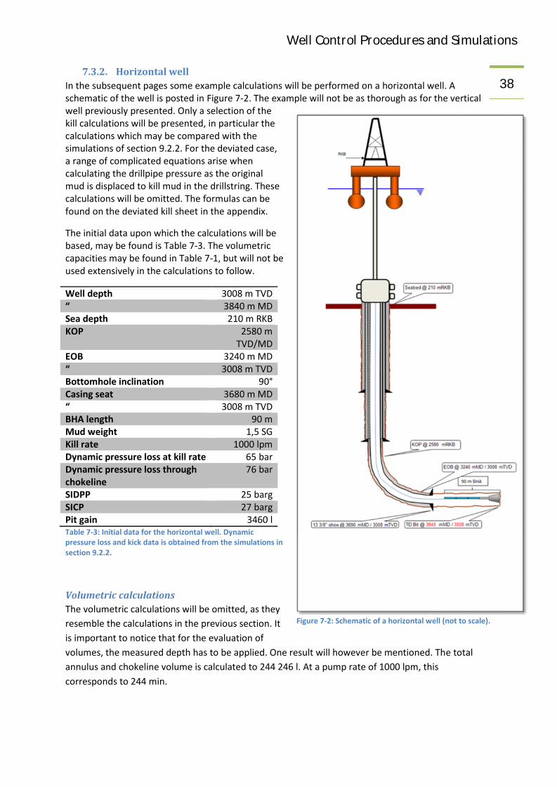
Well Control Procedures and Simulations387.3.2. Horizontal well
In the subsequent pages some example calculations will be performed on a horizontal well. Aschematic of the well is posted in Figure 7-2. The example will not be as thorough as for the verticalwell previously presented. Only a selection of thekill calculations will be presented, in particular thecalculations which may be compared with thesimulations of section 9.2.2. For the deviated case,a range of complicated equations arise whencalculating the drillpipe pressure as the originalmud is displaced to kill mud in the drillstring. Thesecalculations will be omitted. The formulas can befound on the deviated kill sheet in the appendix.
The initial data upon which the calculations will bebased, may be found is Table 7-3. The volumetriccapacities may be found in Table 7-1, but will not beused extensively in the calculations to follow.
Well depth 3008 m TVD“ 3840 m MDSea depth 210 m RKBKOP 2580 m
TVD/MDEOB 3240 m MD“ 3008 m TVDBottomhole inclination 90°Casing seat 3680 m MD“ 3008 m TVDBHA length 90 mMud weight 1,5 SGKill rate 1000 lpmDynamic pressure loss at kill rate 65 barDynamic pressure loss throughchokeline
76 bar
SIDPP 25 bargSICP 27 bargPit gain 3460 lTable 7-3: Initial data for the horizontal well. Dynamicpressure loss and kick data is obtained from the simulations insection 9.2.2.
Volumetric calculationsThe volumetric calculations will be omitted, as theyresemble the calculations in the previous section. Itis important to notice that for the evaluation ofvolumes, the measured depth has to be applied. One result will however be mentioned. The totalannulus and chokeline volume is calculated to 244 246 l. At a pump rate of 1000 lpm, thiscorresponds to 244 min.
Figure 7-2: Schematic of a horizontal well (not to scale).

Well Control Procedures and Simulations39Kick calculations
The influx height may normally be calculated by use of equation (7.18). However, when the well ishorizontal, this approach makes no sense. The vertical height of the kick is limited to the diameter ofthe open hole section. The open hole has a diameter of 12 ¼ inches which corresponds to 0,311 m.
By means of equation (7.19) the influx density is attempted to be calculated.
= -64,0 SG
It is evident that the result is unrealistic. All approaches for estimating the density of the gas isabandoned. Equation (7.15) is used in order to calculate the formation pressure.
= 468 barg
By means of equation (7.16) the necessary kill mud weight is estimated.
= 1,59 SG
The initial circulating pressure, ICP, is calculated by use of equation (7.22).
= 90 barg
In order to calculate the final circulating pressure, FCP, equation (7.25) is utilized.
= 69 barg
Equation (7.12) is used in order to estimate the chokeline friction.
= 11 bar

Well Control Procedures and Simulations40
8. A numerical modelIn order to perform well control simulations, a numerical model was adopted. In the followingsections a brief introduction to the model is given. Further, some modifications are done with thegoal of making the model more suitable and realistic with respect to well control situations. Finally, apresentation of the well control simulations is given. Simulations were conducted on both a verticalwell and a horizontal well.
8.1. Introduction to the numerical modelThe numerical model utilized in this thesis is the drift flux model. The drift flux type models arefundamentally based on a set of three equations. Two of which are relations describing theconservation of mass for the respective phases. The last equation describes the conservation ofmomentum for the combined fluids. In addition, a coupling between the liquid and gas velocities isnecessary. Hence, a slip relation is introduced. The most reasonable results using the drift flux modelare obtained when modeling flow regimes such as dispersed bubble or slug flow[14].
In order to solve the drift flux model a numerical scheme is required. The numerical scheme used inthis thesis is in the family of explicit AUSM schemes (advection upwind splitting method). Thisparticular family of discrete numerical schemes was initially developed by Liou and Steffen[15]. TheAUSM scheme may be utilized to simulate two-phase flow (liquid and gas) in an isothermenvironment. The scheme has been proven to competently model transport of mass as well aspressure pulse propagation in one dimension.
What separates the AUSM schemes from the other numerical schemes is the improved flux splittingscheme derived in [15]. The new flux splitting scheme attempts to combine the advantageousproperties of similar flux splitting methods (FVS/FDS). Further improvements to the flux splittingscheme was proposed by Wada and Liou[16]. This was done for one-phase flow by introducing aconvex combination to the velocity splitting function. The altered flux-splitting scheme eliminatedthe numerical dissipation caused in steady contact discontinuities. Evje and Fjelde[17] followed in thepaths of Wada and Liou, and extended their scheme to applications in a two-phase system. Theresulting model is called AUSMV, and is the scheme utilized in this thesis.
In the following sections the framework of the numerical scheme is outlined. The particular schemepresented in [18] was the starting point of the Matlab code applied in the well control simulations. Itis essentially the same scheme as presented in [17], however the possibility of change in crosssectional area is introduced. Both [17, 18] are valuable references for a more detailed description ofthe AUSMV scheme. Extensions and modifications to the Matlab code for well control purposes arepresented in section 10.3.
8.1.1. Conservation equationsThe conservation equations are the fundament of the drift flux model. There are two equationsdescribing the conservation of mass for the respective phases. A third equation describes theconservation of momentum. Assuming no mass exchange between the phases, this yields thefollowing set of equations,

Well Control Procedures and Simulations41
(8.1)
Where Cross sectional area.
Mass density
Phase velocity
Absolute pressure
Source term, sum of the pressure gradients caused by gravity and friction
The indices l and g represents liquid and fluid. The symbols and corresponds to the derivatives
in time and position respectively. The symbol α denotes the volumetric fluid fractions, with the sumof which equal to unity. Thus, the following relation applies.
(8.2)
These relations are common for all two-phase models derived with basis in the drift flux model.
8.1.2. Mixture propertiesThe volume fractions are further used in describing average properties of the two-phasecombination. The equations describe velocity, density and viscosity, and are all on the same form.The equations are given by,
(8.3)
(8.4)
(8.5)
The viscosities for the one-phase fluids are set to constant values. Liquid viscosity is set to 5 e-2 Pa∙sand gas viscosity set to 5 e-6 Pa∙s. The other parameters are all depending on the dynamic systemproperties.

Well Control Procedures and Simulations42Additionally, an approximation to the sonic velocity of the combined phases is given by,
(8.6)
Where Approximated sonic velocity
Flow dependent parameter (from slip relation, see next section).
In the approximated sonic velocity the K is set to unity. This was done as this was seen to have littleinfluence on the values obtained for the sonic velocities[18].
8.1.3. Slip relationThe slip relation is given by,
(8.7)
Where Concentration profile parameter, set to a constant value of 1,2 (dimensionless)
Drift velocity, set to a constant value of 0,5 m/s
The slip relation is responsible for gas migration and distribution throughout the system. In systemswith a static liquid component, the gas phase will migrate with a velocity just over S. Therefore, S isoften referred to as the drift velocity.
8.1.4. Fluid densitiesThe fluid densities are due to compressibility, functions of pressure. The liquid density function ismodeled by the relation,
(8.8)
Where Liquid density at atmospheric conditions, initially set to 1000 kg/m3
Gauge pressure

Well Control Procedures and Simulations43Sonic velocity in one-phase liquid, set to 1000 m/s
The gas density function is modeled by the relation,
(8.9)
Where Sonic velocity in one-phase gas, set to 316 m/s
8.1.5. The source termThe source term q, on the right hand side of equation (8.1) contains the hydrostatic gravity gradientand the frictional gradient. The gravity gradient is given by,
, (8.10)
Where Acceleration of gravity, 9,81 m/s2
The friction model initially implemented is valid for laminar flow of a Newtonian fluid in a tube ofcircular circumference (section 9.1.6). The friction is given by,
(8.11)
Where Outer diameter (typically open hole diameter or inner diameter of casing)
Friction factor, generally set to 16/Re for laminar flow
The resemblance with equation (7.7) in the analytical model is obvious. However, also a slightly newdefinition of the Reynolds number is introduced:
(8.12)
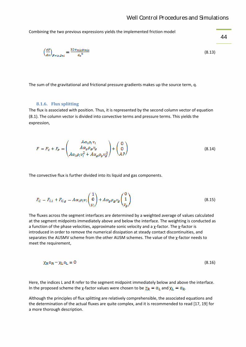
Well Control Procedures and Simulations44Combining the two previous expressions yields the implemented friction model
(8.13)
The sum of the gravitational and frictional pressure gradients makes up the source term, q.
8.1.6. Flux splittingThe flux is associated with position. Thus, it is represented by the second column vector of equation(8.1). The column vector is divided into convective terms and pressure terms. This yields theexpression,
(8.14)
The convective flux is further divided into its liquid and gas components.
(8.15)
The fluxes across the segment interfaces are determined by a weighted average of values calculatedat the segment midpoints immediately above and below the interface. The weighting is conducted asa function of the phase velocities, approximate sonic velocity and a χ-factor. The χ-factor isintroduced in order to remove the numerical dissipation at steady contact discontinuities, andseparates the AUSMV scheme from the other AUSM schemes. The value of the χ-factor needs tomeet the requirement,
(8.16)
Here, the indices L and R refer to the segment midpoint immediately below and above the interface.In the proposed scheme the χ-factor values were chosen to be and .
Although the principles of flux splitting are relatively comprehensible, the associated equations andthe determination of the actual fluxes are quite complex, and it is recommended to read [17, 19] fora more thorough description.

Well Control Procedures and Simulations45
8.1.7. DiscretizationThe time is divided into small timesteps, ∆t. Spatial discretization is conducted in axial direction,where the length of each segment is denoted ∆x. The value of these steps is time and space arerequired to meet the CFL-condition,
(8.17)
For subsonic flow λ1, λ2 and λ3 corresponds to the velocity of the pressure pulses travelling in positiveand negative direction and the fluid velocity.
The set of conservation equations (8.1) can be expressed as,
(8.18)
Introducing the discretization in time and space, and solving for Q at time (n+1) ∆t at segmentnumber I yields the expression,
(8.19)
Here are the fluxes at upper and lower segment interface of segment i.
This particular equation is together with the flux-splitting equations, the core of the Matlab code.These equations are evaluated at every timestep as progress in time is made. This way, the newconserved variables (Qn+1) may be calculated from the old (Qn).
8.1.8. Calculation of primitive variablesThe primitive variables in the new timestep are unknown. There are a total of seven primitivevariables which needs to be calculated:
Volume fractions of the respective phases
Density of the respective phases
Velocity of the respective phases
Pressure
For evaluation of seven variables, a set of seven independent equations is required. The three firstequations are found by using the definition of Q obtained by comparing equations (8.1) and (8.16).

Well Control Procedures and Simulations46(8.20)
In this context, Q is the calculated conserved variable. In addition to the above expression, equations(8.2), (8.7), (8.8) and (8.9) are utilized, in order to evaluate the seven variables.
In the solution strategy implemented in the Matlab code, the pressure is the first variable to beevaluated. The reason for this is that the pressure can be calculated directly from the conservedvariables from the mass conservation. The calculation is done using a second order equation,obtained by combining the above mentioned equations. Knowing the pressure, the density of therespective phases can easily be calculated. This is done using the pressure dependent densityrelations (8.8) and (8.9). This is followed by calculation of the volume fractions and the velocities.
8.1.9. SimplificationsIt is important to realize that the proposed numerical scheme does not describe the real nature of atwo-phase system with total accuracy, nor is it expected to. The concept of finite discretization andnumerical modeling in itself induces inaccuracy. Additionally, a few simplifications must bementioned.
Isotherm system. No mass exchange between the two phases.
However, this numerical scheme is assumed to be a substantially better approximation to realitythan the analytical model proposed in section 7.
8.1.10. RemarksIn the following, a few remarks on the particular numerical scheme and Matlab code are included.They are not of importance for the totality of this thesis, but should be noted for future simulationswith the implemented Matlab code.
Flow related variables which can be altered during a simulationNot all variables can be changed during a simulation run. There are primarily three variables whichcan be continuously controlled:
Liquid mass rate at the inlet (pump rate)
Gas mass rate at the inlet (influx rate)
Pressure at the outlet (choke pressure)
It is recommended to utilize a steady ramp up/down (typically 10 s) if these variables are to bechanged. Rapid changes may induce excessive pressure pulses or water hammering.
Additionally, the outlet can be changed from open/closed (shut-in) or vice versa at any time duringthe simulations.

Well Control Procedures and Simulations47
Initialization of pressure and densityFor a vertical well, the pressures and densities are initialized at standard conditions, and with gravityset equal to zero. During the first 100 seconds of every simulation, the gravity is linearly increasedfrom 0 to 9,81 m/s2. This gives reasonable static pressures and mass distribution throughout thewellbore.
For illustrational purposes, it may be compared to “hoisting” the well from horizontal to vertical.
On the implementation of cross-sectional changesFor the model to function properly, any changes in cross-section have to occur at the segmentmidpoints[18]. This is related to the calculation of the mass fluxes.
For illustrational purposes one-phase simulations were done on a horizontal pipe of length 3000 m.The diameter of the left 1500 m is 0,1 m, while the diameter of the right 1500 m is 0,2 m. A constantliquid mass rate of 10 kg/s was used (from left to right). The first simulation was done with thechange in cross section located at a segment interface (50 segments). The following simulation wasdone with the change in cross section at the segment midpoint (25 segments).
Figure 8-1: Liquid velocities with cross-sectional change in the segment midpoint versus in the segment interface. Thisillustrates the importance of implementing changes in the cross section in the segment midpoints.
The plot shows the steady state velocity profile in the pipe (time 1000 s). The scale on the abscissacorresponds to position relative to the inlet at far left.

Well Control Procedures and Simulations48For incompressible flow, the liquid velocity in a segment should be inverse proportional to the cross-
sectional area of the segment. As seen in the plot, this is clearly not the case when the cross-sectional change occurs in the segment interface.
Velocity profilesThe gravitational term in the equation for momentum conservation seems to cause a slight defect inthe velocity profile of the system. At non-horizontal situations, the velocity in the various segmentsof the well is underestimated. This is most noticeable when the flow rate is set to zero or close tozero. Then, the average velocity in the system becomes negative. Thus, the flow direction isdownwards. In reality, the average velocity should be zero. The error seems to diminish, as thenumber of segments increase.
Figure 8-2: A numerical error causes the fluid velocity profiles to be consistently underestimated. The plot is produced atzero flow rate with increasing discretization. It can be noticed that the fluid velocities approach zero when increasing thenumber of segments.
It is assumed that this effect might be due to numerical dissipation, but the mechanisms behind thisshould be further investigated.
8.2. Development of a crude kick simulatorThe model described in section 8.1 is the starting point in developing a Matlab code for simulationson well control. The main objectives are to make the model more suitable for simulations, and tomake the model more realistic. In order to do this a series of extensions and modifications has to beimplemented:

Well Control Procedures and Simulations49 A more realistic friction model.
Changing the liquid component of the system from water to drilling fluid (altering the liquiddensity).
A backpressure regulator, in order to circulate kicks at constant bottomhole pressure. A more accurate reading of bottomhole and casing pressures. A drillstring function, which makes it possible to read drillpipe pressure. A chokeline and riser for simulation on subsea wells. A pit gain reading. Opening up for wellbore deviation. A Darcy relation for influx where influx size and mass rate depends on downhole pressure
differential. This is important for drilled kicks or connection kicks. Additionally, a choke model was implemented in the model, but it has not been used in the
simulations. The choke model depicts the backpressure as a function of fluid density, flowrate and choke opening.
In the following sections, the implementation of these modifications is described.
8.2.1. Standard test caseA standard test case is introduced in order to verify and compare the modifications done in theMatlab code. The test case is mainly used in sections 8.2.2-3 where nothing else is stated. Thesubsequent modifications are verified by the simulations conducted in sections 8.3 and 8.4. Elementsof the test case will also be referred to in later sections.
Test wellThe simulations to follow are mainly conducted on a common test well of 3000 m. The well is verticalwell with surface BOP. In order to simplify, the borehole has a constant diameter of 12 ¼ in from topto bottom. The well is drilled with 5 inch drillstring and a 180 m 8 ½ inch BHA. The well is divided into25 segments of 120 m.
Test influxA swabbed gas kick of 1867 kg is taken in the test well. The majority of the influx (1600 kg) is takenduring a time period 130-190 s at a constant mass rate of 26,67 kg/s. In addition, there is a 10 s linearramp up/down in both ends of the time interval.
At hydrostatic bottomhole pressure exerted by 1,0 SG mud, the kick mass will occupy on the highside of 6 m3. With 1,5 SG mud it will occupy just over 4 m3.
Time lineThe well is turned to vertical in the first 100 s. The test influx is taken in period 120-200s. Shut-inoccurs at time 260 s, with a 240 s build up of downhole pressures. The kill is initiated at time 500 s ata kill rate of 1000 lpm.

Well Control Procedures and Simulations508.2.2. Friction model
The initial friction model (briefly described in sections 8.1.5) displays excessive oscillation.Additionally, it does not take into account that the flow in a wellbore is annular, nor does it allow forturbulent flow to occur. Two different solutions were proposed and will be tested and compared.The results of the test will result in three alternatives:
Keeping initial model (model #1). Extending initial model to apply for annular flow (model #2). Introducing new model for annular flow, which also takes turbulent flow into account (model
#3).
Model #1As described in the previous paragraph, there are a number of problems associated with the initial
friction model. The friction model displays excessive oscillations. This is assumed to be due to anunrealistically low frictional gradient. If the friction is increased the oscillations are expected to bedamped more rapidly. The friction model utilizes the diameter of the open hole/casing, i.e. the outerdiameter of the annulus. This does not take into account that the flow is annular, and willunderestimate the friction. The model is based on laminar flow, although turbulent flow is known tooccur in a wellbore. This will further underestimate the friction.
Model #2The second model is based on descriptions in [4]. It will make use of equation similar to those ofsection 8.1.5. However, the concept of annular thickness is introduced as an alternative to the outerdiameter used in equation (8.13). This will increase the friction, and is also more realistic than theinitial model. This yields the general expression for the frictional gradient.
(8.21)
The friction factor is still calculated as for laminar flow, and is set to 16/Re. However, the diameter inthe general definition of the Reynolds number is exchanged with the annular thickness. Thus,
(8.22)
Combining equations (8.21) and (8.22) yields the expression,
(8.23)

Well Control Procedures and Simulations51This expression is implemented directly in the source term of the Matlab code.
Model #3Model #3 was suggested in [20], and utilizes annular thickness. Hence, equations (8.21) and (8.22)are valid. The model is also valid for turbulent flow, thus relies on two expressions for the frictionfactor. For laminar flow the friction factor is calculated as,
(8.24)
For turbulent flow, the friction factor is calculated as
(8.25)
The model uses Re=2000 as the upper limit for laminar flow. Lower limit for turbulent flow is set atRe = 3000. In the transition between laminar and turbulent flow linear interpolation is applied inorder to obtain a smooth transition.
This model is implemented in the Matlab code as a function which calculates the frictional gradient insteps. Therefore, the explicit expressions for the frictional gradient will not be presented here.
Model testing and resultsThe testing is performed on the standard test case defined in section 8.2.1. During the circulation,the outlet pressure is kept at a constant level equal to SICP.
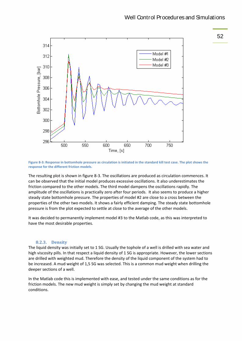
Well Control Procedures and Simulations52
Figure 8-3: Response in bottomhole pressure as circulation is initiated in the standard kill test case. The plot shows theresponse for the different friction models.
The resulting plot is shown in figure 8-3. The oscillations are produced as circulation commences. Itcan be observed that the initial model produces excessive oscillations. It also underestimates thefriction compared to the other models. The third model dampens the oscillations rapidly. Theamplitude of the oscillations is practically zero after four periods. It also seems to produce a highersteady state bottomhole pressure. The properties of model #2 are close to a cross between theproperties of the other two models. It shows a fairly efficient damping. The steady state bottomholepressure is from the plot expected to settle at close to the average of the other models.
It was decided to permanently implement model #3 to the Matlab code, as this was interpreted tohave the most desirable properties.
8.2.3. DensityThe liquid density was initially set to 1 SG. Usually the tophole of a well is drilled with sea water andhigh viscosity pills. In that respect a liquid density of 1 SG is appropriate. However, the lower sectionsare drilled with weighted mud. Therefore the density of the liquid component of the system had tobe increased. A mud weight of 1,5 SG was selected. This is a common mud weight when drilling thedeeper sections of a well.
In the Matlab code this is implemented with ease, and tested under the same conditions as for thefriction models. The new mud weight is simply set by changing the mud weight at standardconditions.
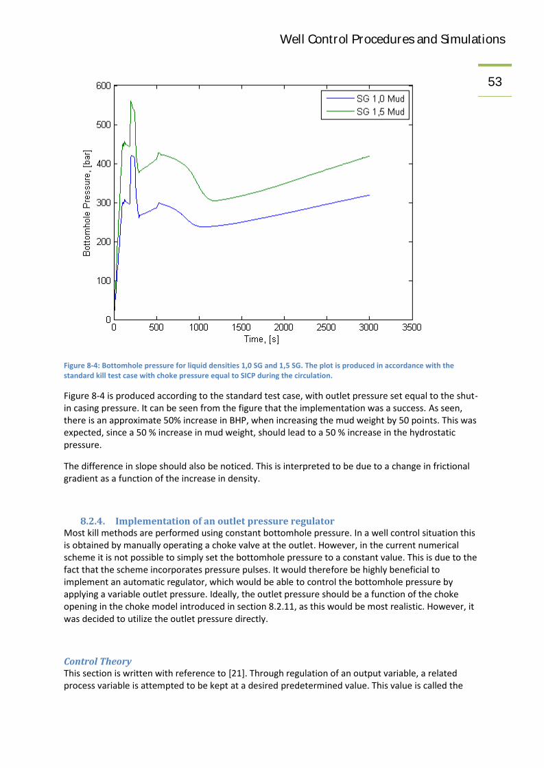
Well Control Procedures and Simulations53
Figure 8-4: Bottomhole pressure for liquid densities 1,0 SG and 1,5 SG. The plot is produced in accordance with thestandard kill test case with choke pressure equal to SICP during the circulation.
Figure 8-4 is produced according to the standard test case, with outlet pressure set equal to the shut-in casing pressure. It can be seen from the figure that the implementation was a success. As seen,there is an approximate 50% increase in BHP, when increasing the mud weight by 50 points. This wasexpected, since a 50 % increase in mud weight, should lead to a 50 % increase in the hydrostaticpressure.
The difference in slope should also be noticed. This is interpreted to be due to a change in frictionalgradient as a function of the increase in density.
8.2.4. Implementation of an outlet pressure regulatorMost kill methods are performed using constant bottomhole pressure. In a well control situation thisis obtained by manually operating a choke valve at the outlet. However, in the current numericalscheme it is not possible to simply set the bottomhole pressure to a constant value. This is due to thefact that the scheme incorporates pressure pulses. It would therefore be highly beneficial toimplement an automatic regulator, which would be able to control the bottomhole pressure byapplying a variable outlet pressure. Ideally, the outlet pressure should be a function of the chokeopening in the choke model introduced in section 8.2.11, as this would be most realistic. However, itwas decided to utilize the outlet pressure directly.
Control TheoryThis section is written with reference to [21]. Through regulation of an output variable, a relatedprocess variable is attempted to be kept at a desired predetermined value. This value is called the

Well Control Procedures and Simulations54setpoint. In this case, the output variable will be the outlet pressure (choke pressure). The variable to
remain constant will be the bottomhole pressure.
A general PID-regulator (proportional, integral, derivative) continuously gives the output variable asthe sum of three main terms.
The proportional term. The integral term. The derivative term.
The proportional term contributes to the output variable with a value proportional to the deviation(error, denoted e) between the setpoint and the actual process variable at any given time. Theproportionality factor is called the proportional gain and denoted Kp. In this context the setpoint willbe the bottomhole pressure measured at shut-in, the process variable will be the measuredbottomhole pressure.
The integral term is meant to assure that the errors accumulated in time will approach zero. This isachieved by adding a contribution to the output variable, equal to the time integral of the errormultiplied by a factor. The factor is called the integral gain, and is equal to the proportional gaindivided by the integral time (Kp/Ti).
The derivative term intends to compensate for sudden changes in the process variable. Thederivative term contributes to the output variable with a value proportional to the time derivative ofthe error. The proportionality factor is called the derivative gain, and can be further decomposed tothe proportional gain multiplied with the integral time (Kp Td).
An optional parameter called the nominal output (uo) may be added to the PID-regulator. This is setat a value in the same range in which the output variable is expected to vary.
The proportional gain, integral time, derivative time and the nominal output must all be tuned inorder to achieve optimal regulation. This is achieved using Ziegler-Nichols' closed circuit method,described in the appendix. The tunable parameters have to be adjusted for every change in processdynamics (kick size, well depth, fluid properties etc.).
The PID-regulator is generally given by the expression,
(8.26)
Where Output variable, in this case outlet pressure
Nominal output, in this case set to SICP
Error, the difference between the setpoint and the process variable
Time
Proportional gain
Integral time

Well Control Procedures and Simulations55Derivative time
Equation (8.26) is based on a continuous scale, both in time and space. However, in the numericalscheme, time and space are discrete. Thus, equation (8.26) has to be converted to discrete form. Theintegral term is therefore implemented as a sum, and the derivative as a difference. The formulathen takes the form
(8.27)
The regulator may also take an equivalent form, by subtracting u(t-1) from u(t), so that
(8.28)
Where Sample time, the period in time between every adjustment in the output variable. Set
to dt where nothing else is stated.
Equations (8.27) and (8.28) are both implemented in the Matlab code, and yields equivalent results.
If satisfactory regulation is not achieved after tuning the parameters according to Ziegler-Nicholsroutine, it is suggested to scale the regulator parameters by multiplying them with a common factor.This is done as a means for adjusting the rate of convergence or the stability of a regulator. That is,Kp, 1/Ti and Td may be adjusted by a factor c, so that
(8.29)
In order to increase the convergence rate of the regulator, c is set to a value greater than 1. In orderto improve the stability, c is set less than 1. However, c should not be set to a negative value, as thiswill make the proportional term counteract the convergence of the bottomhole pressure. By settingc=1, the regulator parameters remains unchanged. Setting c=0 will simply reduce the regulatoroutput to the nominal output uo.

Well Control Procedures and Simulations56Complications
The design of a choke regulator is a challenge, due to the complexity of the wellbore system. There isa time lag between any pressure regulation on top and the following response in bottomholepressure. This time delay is not only dependent on the measured well depth, but also on the volumefractions and variable properties of the respective fluids.
Another complicating factor is that the bottomhole response of a choke pressure adjustment isvariable throughout a round of circulation of a kick. This is due to gas expansion, which leads toincreasing volume fractions of gas in the wellbore. The gas acts as an accumulator which partiallyabsorbs any choke pressure adjustment.
Rapid manipulation of the choke pressure will induce oscillating pressure pulses in the wellboresystem. This may result in over-compensating the output pressure.
Regulator tuningThe implemented PID-regulator is tuned using Ziegler-Nichols' closed circuit method, described in theappendix. Initially, three approaches were considered for the purpose of tuning the regulator:
Tuning the regulator with respect to an increase in pump rate in a liquid filled well.
Tuning the regulator with respect to an increase in pump rate in a well partially filled withgas.
Tuning the regulator with respect to a well control situation.
In all cases the test well introduced in section 8.2.1 is considered. The outlet regulator commencesfrom time 500 s.
In the first two cases an increase in bottomhole pressure was induced by going from static conditionsto a 5000 lpm pump rate. The volume rate is applied from time 500 s, and yields an increase inbottomhole pressure of just more than 1 %. The nominal output pressure is set to 1 bara, and the setpressure was set to 438,8 bara (approximately 1 bar below the hydrostatic pressure). The firstapproach is conducted in a well completely filled with drilling fluid. For the second approach, the wellwas initialized (before turned to vertical) with a 0,1 volume fraction of gas. For the third approach,the full test case outlined in section 10.2.1 was conducted.
By an application of Ziegler-Nichols routine, the critical values Kpk and Tp were found, and from thesethe tuned parameters were obtained. The results are presented in the table below.
Approach # Regulator Kp Ti, [s] Td, [s]1 PID 0,6 3,0 0,75“ PI 0,45 5,0 02 PI 0,405 6,67 03 PI 0,135 12 0Table 8-1: Tuned regulator parameters for the various approaches.

Well Control Procedures and Simulations57
Figure 8-5: PI-regulator tuned with respect to approach #1 compared with non-regulated bottomhole pressure. Pressureresponse as pump rate is raised from 0 to 5000 lpm at time 500 s.
The figure above is produced with basis in the first approach. It displays the PI-regulator with theparameters as stated in the table. It is observed that the PI-regulated bottomhole pressuresuccessfully converges towards the setpoint. Another observation is that the regulator operates withnegative outlet pressures. This was later altered, and an upper and lower limit for the outlet pressurewas introduced. The lower limit is the atmospheric pressure, 1 bar. The upper limit is set to 1035 bar,which corresponds to a choke valve pressure rating of 15000 psi. This is a typical value used on highpressure equipment.
The PID-regulation was not included in the figure due to instability and excessive oscillations. Thehigh amplitudes were not only caused by pressure pulses, but also regulator instability. It wasassumed that some of the instability was caused by the derivative term of the regulator. In thefurther work it was decided to completely abandon the PID-regulation, and focus on PI-regulation.
The plot produced from the second approach will not be presented here, as it is resembles Figure8-5. The figure obtained from the third approach will be presented in the next section, where it alsowill be compared with the two previous approaches.
Regulator testingFurther, the tuned regulators obtained from the different approaches were tested and compared in atest case. However, a mistake was made, and the actual test case deviates slightly from the casedefined in section 10.2.1. The main difference from the defined test case is that the bottomholepressure is read from the bottom of segment one instead of in the midpoint (see section 10.2.5),while the regulator operates with respect to the segment midpoint. Additionally, the length of the

Well Control Procedures and Simulations58BHA is set to 300 m, as opposed to 180 m for the defined test case. This deviation from the standard
test case is not expected to cause a degradation of the qualitative results of the test. Quantitativelyhowever, this will affect the downhole pressures throughout the simulation runs.
The nominal output pressure was set equal to the shut-in casing pressure. For the setpressure, avalue equal to the shut-in bottomhole pressure was utilized.
Figure 8-6: Testing of the PI-regulators tuned with respect to the various approaches. The regulators are tested in a wellcontrol situation slightly deviating from the standard test case.
The results of the testing may be seen in the figure above. All regulators functioned satisfactory inthe time before 2100 s. However, it can be seen that the regulators tuned with respect to the firsttwo cases displayed substantial instability from time 2100 s. After analysis of the gas/liquid fractionprofiles, it was discovered that this coincides with the time in which the gas approaches the surface.The massive gas expansion close to surface, challenges the dynamic properties of the regulator. Thismeans that the tuning of the regulator parameters is not optimal, with respect to a situation withlarge amounts of gas present.
The root mean square of the error was calculated for the different approaches. For the respectiveapproaches the values were found to be 9,76 bar, 9,19 bar and 4,81 bar (approach #1, approach #2and approach #3 respectively). As might be expected and as seen in the figure above, the regulatortuned directly with respect to the kill situation displayed the best performance. The performance ishowever not satisfactory. Thus, it was decided to scale the parameters found from the thirdapproach, in accordance with equation (8.29).

Well Control Procedures and Simulations59Scaling the regulator parameters
Using the tuned parameters found by approach #3 (Kp=0,135; Ti=10), a range of different scalingfactors were tested. This was done in order to investigate the effect with respect to stability and rateof convergence. The ultimate objective is to make the regulator perform with a high rate ofconvergence while still maintaining satisfactory stability. The scaled regulators were tested accordingto the standard test case defined in section
8.2.1
Figure 8-7: Regulator parameters from approach #3 scaled with a range of different scaling factors c. The performance ofthe scaled regulators is tested according to the defined standard kill test case from section 8.2.1.
As can be seen in the figure, the scaling of the parameters by a factor c, affects the variable pressuresas previously claimed. Increasing c, yields a higher rate of convergence on the expense of loosingstability and vice versa. Simulations were also run for scaling parameters higher than 1,3. These arehowever not included in figure 8-7, as heavy oscillations occurred.
c 0,8 1,0 1,2 1,3 1,4 1,6RMS, [bar] 3,29 2,38 1,88 1,72 1,98 3,15Table 8-2: Root mean square of the error (e), for the various scaling parameters in Figure 8-7.
In Table 8-2 the root mean square of the error for the different scaling factors are to be found.Looking at the table, the lowest RMS value is found for c=1,3. Hence, this may be looked upon as thebest scaling factor. However, considering Figure 8-7, sustained oscillations occur around time 2250 swith the particular scaling factor. The damping of the initial oscillations is also poor. Thus, a value of1,3 were in this case assessed as to be too high. The most convergent regulator, while stillmaintaining sufficient stability is found for c=1,2.
Even though the scaled regulator performed decent, the maximum bottomhole pressure after theinitial oscillations are damped is 449,5 bar, the minimum pressure is 444,2 bar. This means the

Well Control Procedures and Simulations60interval in which the error e varies is reduced from 7,4 to 5,3 bar with respect to c=1. This is however
still not satisfactory regulation. In traditional control theory, the next step in improving theregulation is gain scheduling. This approach will not be attempted in this thesis, as it is expected tobe a fairly time consuming process. However, a novel approach was discovered, which displayedbetter properties. This will be introduced in a subsequent section.
Altering the sample timeIn the previous regulators the outlet pressure was altered in every timestep (Ts=dt). It was decided
to investigate if increasing the sample time would improve the properties. The regulator parametersare tuned for every different sampletime. The tuned parameters are found in Table 8-3.
Ts, [s] Kp Ti, [s] cdt 0,135 10 1,23dt 0,135 10,83 1,21 0,09 11,67 1,23 0,09 12,5 1,2Table 8-3: Optimally tuned regulator parameters.
Figure 8-8 is produced by using the optimized parameters for the various sample times. The testing isconducted on the defined standard kick case (section 8.2.1).
Figure 8-8: PI-regulation with increasing sample time. Testing conducted on the defined standard kick case.
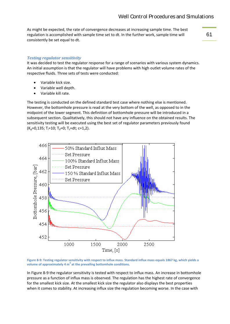
Well Control Procedures and Simulations61As might be expected, the rate of convergence decreases at increasing sample time. The best
regulation is accomplished with sample time set to dt. In the further work, sample time willconsistently be set equal to dt.
Testing regulator sensitivityIt was decided to test the regulator response for a range of scenarios with various system dynamics.An initial assumption is that the regulator will have problems with high outlet volume rates of therespective fluids. Three sets of tests were conducted:
Variable kick size. Variable well depth. Variable kill rate.
The testing is conducted on the defined standard test case where nothing else is mentioned.However, the bottomhole pressure is read at the very bottom of the well, as opposed to in themidpoint of the lower segment. This definition of bottomhole pressure will be introduced in asubsequent section. Qualitatively, this should not have any influence on the obtained results. Thesensitivity testing will be executed using the best set of regulator parameters previously found(Kp=0,135; Ti=10; Td=0; Ts=dt; c=1,2).
Figure 8-9: Testing regulator sensitivity with respect to influx mass. Standard influx mass equals 1867 kg, which yields avolume of approximately 4 m3 at the prevailing bottomhole conditions.
In Figure 8-9 the regulator sensitivity is tested with respect to influx mass. An increase in bottomholepressure as a function of influx mass is observed. The regulation has the highest rate of convergencefor the smallest kick size. At the smallest kick size the regulator also displays the best propertieswhen it comes to stability. At increasing influx size the regulation becoming worse. In the case with

Well Control Procedures and Simulations62the highest influx mass, regulator instability occurs as gas reaches the surface. This agrees with the
initial assumption.
Figure 8-10: Testing regulator sensitivity with respect to well depth. The vertical geometry of the standard test well hasbeen elongated and contracted. The bottomhole pressure has been normalized by dividing with the set pressure. This isdone to get the testing results in the same frame of reference.
Figure 8-10 is the result of a set of tests for finding the sensitivity of the tuned regulator with respectto well depth. In order to present the bottomhole pressures in the same frame of reference, theyhave been divided with the respective set pressures.
The properties with respect to rate of convergence and stability are best for the deeper wells. For the2000 m well, excessive oscillations occur as gas reaches the surface. As the influx mass is the same inall three simulations, this is interpreted as an effect of gas distribution. In the shallow well, the gaswill reach surface before it has been properly distributed. In the deeper wells the distribution profileof the gas will be more elongated due to migration and gas slippage. Thus, the volumetric rates ofgas will be lower as it reaches surface. This supports the initial assumption.

Well Control Procedures and Simulations63
Figure 8-11: Testing regulator sensitivity with respect to kill rate.
In Figure 8-11 the results from the sensitivity tests with respect to varying pump rate are shown.Unexpectedly, the stability decreases at lower volume rates out. This is in contradiction with theinitial assumption, and should be further investigated.
A novel approachAccording to classical control theory, the next step in improving the regulation convergence andstability is gain scheduling. However, a new approach is suggested. The constant nominal output inthe PID regulator is replaced with a variable reflecting the changes in dynamic properties, as the gasbubble rises in the annulus. By simply replacing the nominal output, with the output value at time t-1, impressive regulation was accomplished. This yields the relation,
(8.30)The reasons for the success of this approach and its further implications, are not fully understood,and should be investigated.
The regulator was tuned by the same routine as done in previous sections. Satisfactory stability maybe achieved by reducing the proportional gain by three orders of magnitude, compared to the typical

Well Control Procedures and Simulations64proportional gains used in the previous sections. At sample time dt, critical proportional gain is found
to be 0,0011. The critical period is 19 s. The tuned regulator parameters are therefore set to Kp=4,95· 10-4 and Ti=15,83 s according to Ziegler-Nichols. The optimal scaling factor c was found to be 1,1.
The new regulator was compared with the tuned regulator obtained from the classical approach. Thestandard test case was run using bottomhole pressure measurement in the midpoint of thelowermost segment.
Figure 8-12: Tuned new approach tested against tuned classical approach. The testing was conducted on the standardtest kick situation.
Using the new approach and after the initial oscillations are damped, the bottomhole pressure variesin an interval of 0,8 bar around the setpressure, whereas the corresponding interval of the classicalapproach is 5,3 bar. The respective root mean square of the error is 1,36 bar and 1,88 bar. This is asignificant improvement. It seems that the new approach handles the dynamic nature of the kicksituation in a better manner. Similar results could possibly also be achieved using classical controltheory and gain scheduling. However, the new approach is less time consuming, while yet producessatisfactory regulation. Hence, the new approach will be used in the kick simulations to follow.
8.2.5. Accurate pressure readingsThe bottomhole pressure initially read in the model is actually a pressure reading at the midpoint ofthe bottom segment. For a 3000 m well divided into 25 segments, this corresponds to a pressurereading 60 m off bottom. A more accurate pressure reading was desired. This was obtained by linearinterpolation.

Well Control Procedures and Simulations65
Where True Bottomhole Pressure
Pressure at midpoint of segment 1
Pressure at midpoint of segment 2
This equation neglects any difference in pressure gradient in the 1 1/2 bottom segments. Thus, it isassumed that the volume fractions, fluid velocities and densities are equal in the segments. Theseassumptions might produce a slight error. However, the error will diminish if the segment length isallowed to approach zero.
The same correction was made for the choke pressure.
8.2.6. Implementation of drillstringThe most important topside pressure when it comes to well control situations is the drillpipepressure. The pressure is applied the kill sheet, and is also the parameter used in order to control thebottomhole pressure during the kill circulation. The drillpipe pressure is measured at drill floor level,at the standpipe manifold. It would be useful to have a drillpipe pressure reading implemented in theMatlab code.
A rather simple drillpipe pressure function was implemented. It is directly deduced from thebottomhole pressure, and does not take into account the time delay in the pressure response, northe acceleration terms found in the AUSM model. The implemented drillpipe pressure is a function ofa constant hydrostatic head of the mud column contained in the drillstring, and the friction loss dueto mud flow. Further, a pressure loss across the drill bit was added. The entire drillstring wasmodeled as one segment, and constant capacity of the drillstring was assumed to be 8 l/m. Thiscorresponds to an inner diameter of 0,10 m. The concept of the function may be stated as,
(8.31)
Where the denotation is as described in section 7.1.3.
Hydrostatic pressureThe hydrostatic pressure in the drillstring is awkward to model. Simply setting the mud weight in thedrillstring to 1,5 SG will cause a to high drillpipe pressure, as the mud on the annulus side iscompressible. The average mud weight on the annulus side is higher than 1,5 SG. The selectedsolution is to make use of the bottomhole pressure measured after the well is turned to vertical.Immediately after the well is turned to vertical, the bottomhole pressure will exhibit exponentiallydamped oscillations, converging towards a value of hydrostatic pressure. An attempt was made tofind the correct value of hydrostatic pressure, by averaging the oscillations over time. This wouldmake the model flexible with respect to changes in density or well depth. However, this proved

Well Control Procedures and Simulations66difficult, as the hydrostatic bottomhole pressure was slightly overestimated. Other attempts were
made to weight the average in various ways, so that the values produced with the lowest amplitudeswas emphasized. It was also attempted to average the maximum and minimum values of theoscillations, and the values at the inflection points. None of these strategies were successful. Finally,a simulation was run to 1000 s, using no downhole inlet rates, nor any manipulation of chokepressure. The bottomhole pressure was converged to a constant value of 448 bar. This value was setconstant in the drillpipe model. However, in reality the average density is a function of the pressure,so that the hydrostatic pressure would increase when subjected to pump pressure. This effect wasneglected, but the resulting errors are assumed to be small, as the drilling fluid is close toincompressible.
FrictionFor friction, the function implemented in section 8.2.2 was utilized. Only the input parameters arechanged. The liquid density may be derived from the hydrostatic pressure. It is obtained by dividingthe hydrostatic pressure by the well depth and the gravity acceleration. This yields an averagedensity of approximately 1,52 SG. The liquid velocity is set to liquid mass flow rate divided by theaverage density derived from the hydrostatic pressure. This is again divided by the capacity of thedrillpipe to obtain velocity. The liquid volume fraction in the drillstring is set to 1. This is realistic, asthere normally is a float valve in the BHA, so that flow of gas into the drillstring is prohibited. Thepressure input is set to the average between the drillpipe pressure and the bottomhole pressure. Thediameter is set to correspond with the capacity of the drillpipe. The viscosity is set to 0,05 Pa*s.
Pressure drop across bitThe pressure drop across the bit was obtained as described in section 7.1.7.
The cross-sectional area of the bit nozzles is set to 0,902 square inches, with reference to the BHApresented in the appendix. In SI units this corresponds to 5,82 * 10-4 m2. This is assumed to be atypical value. The discharge coefficient C, depends on the design of the nozzle, but is set to 0,95 withreference to [5].
8.2.7. Implementation of chokeline and riserAn offshore well with a subsea BOP, has a chokeline and riser which connects the BOP to the surfacedrilling facilities. During normal drilling operations, mud returns are taken through the riser.However, in a well kill scenario, the BOP will be closed, and the circulation will take place through achokeline to the choke manifold. The chokeline has a small diameter, and acts itself as a choke valvedue to friction loss. Typical inner diameters of the riser and chokeline are 18 ¾ inch and 3 inch.
In order to simulate well control procedures with a subsea BOP, a chokeline and riser had to beimplemented. The intention was to let the wellbore branch into two different sets of segments fromseabed to drill floor. The flow was to be controlled during simulations by operating a failsafe valve inconjunction with the BOP. Closed BOP and open failsafe valve would direct the flow through thechokeline, open BOP and closed failsafe would direct the flow through the riser. However, this wasproven to be a quite cumbersome task, with respect to boundary conditions and fluxes at thesegment boundaries. It was therefore decided to initialize the well with the desired geometry(chokeline or riser), rather than being able to manipulate the failsafe valve during simulations. Thus,there is no possibility of changing flow path between riser and chokeline during simulations, norshutting in the well at seabed. This reduces the flexibility of the model. However, it may be assumedthat the shut-in pressures below seabed should remain equal, whether the actual point of shut-in is

Well Control Procedures and Simulations67situated at surface or seabed. This assumption is valid as long as the effect of pressure pulses is
negligible, and as long as the influx is situated below seabed.
The kill simulations to follow are run in two sequences. First a shut-in sequence with returns throughriser. All data from the shut-in sequence is exported, except the conservative variables and thegeometric data, and the simulations continued with failsafe open, i.e. with returns through thechokeline.
For convenience, a pressure recording at seabed was implemented. It is found by linear interpolationbetween the pressures read at the midpoint above and below the segment boundary correspondingwith the seabed.
8.2.8. Implementation of pit gainAfter a kick has been taken and the well is shut-in, the pit gain is read. This parameter is an indirectmeasurement of the influx size, and is used to calculate the kick height and the kick’s averagedensity. In that sense, it is an important parameter.
A pit gain monitor was implemented. The pit gain equals the time integral of the liquid volumetricflow rate at the outlet subtracted liquid volumetric flow rate into the hole. The integral is set to zerofor at least the first 100 s of the simulations, as there occurs a negative outlet rate due to liquidcompression when the well is hoisted to vertical.
8.2.9. Implementation of wellbore deviationIn order to be able to perform simulations on non-vertical wells, every segment was assigned anaverage angle (in radians). This angle is generated automatically, by setting a kick off point, an end ofbuild and a final bottomhole inclination angle. The cosine of the various inclination angles were alsointroduced in the gravitational term in the conservation of momentum equation. Furthermore, slightchanges had to be done in the drillstring function. The mean density of the drilling fluid in thedrillpipe has to be calculated as a function of true vertical depth, rather than measured depth.
The slip-relation which was introduced in the previous sections is valid for vertical flow (inclinationangle = 0). For horizontal flow, no-slip was assumed (inclination angle = π/2). For inclination angles inbetween, there was assumed a relation proportional to cosine of the angle of inclination. Thus,
(8.32)
This relation yields zero drift velocity s, at horizontal sections. This is a reasonable assumption sincethe drift velocity of the gas phase is a function of buoyancy. Buoyancy is directed upwards, thus thedrift velocity should be directly proportional with the vertical component of the segment length.
8.2.10. Implementation of Darcy relation for influxThe previous simulations on kicks were made with gas influx rates reminiscent of swabbed kicks. Theinflux rate was slowly ramped up to a predefined influx rate. After the desired kick volume was

Well Control Procedures and Simulations68present in the lower segments of the wellbore, the influx rate was again ramped down to zero. This
corresponds to pulling out pipe at slow rate, and stopping for connection.
The further simulations will be performed on drilled kicks. In order to get a realistic pressure buildup, a pressure dependent influx relation has to be implemented. According to Darcy’s law forpseudo-steady state[13], the influx rate is proportional to the formation pressure squared subtractedthe bottomhole pressure squared. Thus
(8.33)
Where mass flow rate
By assuming a constant formation pressure larger than the hydrostatic pressure of the mud column,and a reference flow rate at known bottomhole pressure (here equal to the hydrostatic pressure), aninflux relation may be established. This yield,
(8.34)
Where Reference flow rate (at bottomhole pressure equal to hydrostatic), set to 10 kg/s
Absolute hydrostatic pressure exerted bottomhole
Formation pressure, set to 475 bara
The reference flow rate will depend on the pressure drawdown between the formation and thewellbore (kick intensity), and on the area of the wellbore/formation interface. It will also depend onthe viscosity of the formation fluid and the formation properties (geometry, permeability).
The influx rate has to be gradually ramped up in order to avoid water hammering and seriouspressure oscillations. The influx will cease when the well is shut in, and bottomhole pressure equalsformation pressure.
8.2.11. Implementation of a choke modelIn section 8.2.4, the choke back pressure has been regulated directly by setting a value for thepressure at the outlet. This is however a rather artificial concept. In reality, the back pressure isregulated by a choke valve. Therefore, a choke valve was implemented in the model. The relationdefining the choke valve is equation 7.14. The pressure response in the choke valve depends on theopening in the choke, and is given in terms of a fraction, where 1,0 is fully open and 0,0 is fully

Well Control Procedures and Simulations69closed. However, the choke setting may never equal 0, as the outlet pressure then will approach
infinity. This will require a different set of boundary conditions.
The choke valve is implemented in the Matlab code, but has not been used in the simulations tofollow.
9. SimulationsIn the following sections some simulations will be run, predominantly well control simulations on onevertical well and on one horizontal well. First however, a few initial simulations will be conducted.
9.1. Initial simulationsInitially a few simulations were run, partly in order to test the scheme, partly to look at some physicalproperties of the two-phase system. Some of these cases are vital for the analysis of the well controlsimulations in section 9.2. The initial simulations are kept as simple as possible, in order toinvestigate the particular effects. A 3000 m pipe of a uniform diameter of 0.1 m was considered. Thepipe was divided into 25 segments, and the timestep was set to 0,025 s.
9.1.1. CompressibilityA 3000 m open ended vertical pipe is considered. An outlet pressure of 500 bara was applied fromthe very beginning. From time 500 s the pressure was ramped down in steps of 100 bar, 100 s foreach step, until finally 0 bara of backpressure was applied on the top. The simulation was run untiltime 1200 s. Two different cases are considered.
Static, liquid filled pipe.
Static, gas filled pipe. Slip relation was set to no slip.

Well Control Procedures and Simulations70
Case #1
Figure 9-1: Liquid density throughout the wellbore as a function of increasing pressure. Liquid density at standardconditions is 1500 kg/m3.
From Figure 9-1 it is evident that the density of a liquid is very dependent on the prevailingpressures. An increase in
Case #2The attempt was a failure, as there seems to be a numerical problem.
9.1.2. Pressure pulseA 3000 m open ended horizontal pipe is considered. Two different cases are investigated.
Static, liquid filled pipe. Pressure pulse induced by rapid increase in outlet pressure. Static, partially gas filled pipe with a 0,5 volume fraction of gas (no-slip). Pressure pulse
induced by rapid increase in outlet pressure.
Case #1At time 250 s the pressure is ramped up from 1 to 11 bara in a one second interval.

Well Control Procedures and Simulations71
Figure 9-2: Pressure pulses produced in liquid filled pipe by a rapid increase in outlet pressure from 1 bara to 10 bara. Thepipe is horizontal with an open end.
Figure 9-2 illustrates a pressure pulse in a liquid filled horizontal pipe with an open end. It is evidentthat the pressure pulses cause excessive oscillations in pressure. The oscillations are more violentfurther from the outlet. The maximum and minimum pressure at the inlet is respectively 17,0 baraand 8,7 bara (water hammering effect). The oscillations are exponentially dampened due to friction,and the inlet pressure stabilizes at 11 bara around time 340 s, 90 s after the occurrence of thepressure shock.
During further analysis of the inlet pressures, it was discovered that the first incremental pressureincrease (0,001 bar) at the inlet occurs 1,9 s after the pressure shock has been applied at the outlet.The vertical displacement between the outlet and the pressure recording at the inlet is 2940 m. Thesonic velocity in one phase liquid is 1000 m/s. Thus, a pressure increase should first be observed atthe inlet 2,9 s after the pressure shock occurred. The reason for this is not known, and it should beinvestigated further.
It was found that the average oscillation period at the inlet for the four first oscillations is 11,8 s. Thisis close to four times the expected pressure pulse propagation time (one way). It is expected that thisis due to the fact that two pressure waves are propagating in opposite direction. This may cause theperiod of the amplifications (both pressure waves on top of one another) to be misinterpreted as theperiod of oscillation.
Case #2The same rapid increase in pressure was applied to a system containing 0,5 volume fraction of gashomogeneously distributed. No slip was assumed as the system is horizontal. Hence, the slipparameters were adjusted to k=1 and s=0.

Well Control Procedures and Simulations72
Figure 9-3: Pressure pulse produced by a rapid increase in outlet pressure from 1 bara to 11 bara. A horizontal pipe isinitially filled with 0,5 volume fraction liquid and 0,5 fraction of gas. (As pressure increase the volume fraction of gas willdecrease.) The pipe is open ended at the endpoint of segment 25.
Figure 9-3 displays the pressure propagation in a partially gas filled horizontal pipe. It can beobserved that the pressure wave travels at a very low velocity. An initial incremental increase inpressure (0,001 bar) at the inlet is first recorded at time 390 s. This is 140 s after the pressure shock isapplied at the outlet. This yields a sonic velocity of 21 m/s, and is due to a reduced sonic velocity inthe two-phase mixture. One phase gas velocity is set to 316 m/s while the corresponding for gas is1000 m/s.
The simulation was continued to 5000 s in order to establish if there would be any furtheroscillations. It was however found that the outlet pressure stabilized at 11 bara without any kind ofoscillation. This occurred at time 1500 s.
9.2. Well control simulationsIn this section, the results of the conducted well control simulations will be briefly presented. Thesimulations will be done in two different subsea wells, one vertical and one horizontal. These wellsare the same as those introduced in the example calculations in sections 7.3.1 and 7.3.2. Fourdifferent sets of simulations will be run for each well.
SCR
Shut-in
Partial kill using Driller’s Method

Well Control Procedures and Simulations73 Worst case
The primary objective for the SCR simulations is to obtain a value for the dynamic pressure lossthrough the chokeline and through the riser. The values for dynamic pressure loss are found bysubtracting the atmospheric pressure from the dynamic drillpipe pressure. These values are furtherused in the example calculations in sections 7.3.1 and 7.3.2. In this way, the example calculations andthe simulated kill will be directly comparable. Additionally, the respective loss components(drillstring friction, pressure loss across bit, annular friction and friction loss in chokeline/riser) will bemeasured. This will give an illustration of the distribution of pressure loss with respect to the variouspressure loss components. The sum of the loss components should ideally match dynamic drillpipepressure.
The main purpose of the shut-in simulation is to provide the shut-in pressures and pit gain for the killcalculations in sections 7.3.1 and 7.3.2. Further, the shut-in sequence serves as a basis for the killsimulations and partially the worst case simulations.
The partial kill simulations are executed in order to verify the analytical model and the kill sheet, andto detect any flaws in the kill procedures. The partial kill features the first round of circulation usingDriller’s Method. Thus, the kick is circulated to surface using the original drilling fluid. The PI-regulation is conducted with respect to the drillpipe pressure. This is done for the purpose of realism.
Two worst case simulations will be run for each well. One reflects the conventional worst casescenario (approach #1) as defined in section 3.1.2. This will be directly comparable with the examplecalculations in section 7.3.1. Another scenario was considered, with a slug of gas migrating in a shut-in well (approach #2). The comparisons are to be found in section 0.
For the well control simulations, the timestep is set to 0,0125 s and the well divided into 50segments. This is done in order to increase the accuracy of the simulations.
9.2.1. Vertical wellA 3000 m RKB vertical well was initialized. The 13 3/8 inch (ID = 32 cm) casing shoe is situated at2850 m, and the remaining 150 m consists of 12 ¼ inch open hole. Water depth is 210 m RKB, with 18¾ inch riser and 3 inch chokeline. The drillstring is composed of 5 inch drillpipe and a 90 m 8 ½ inchBHA. The capacity in the drillstring is assumed to be 8 l/m, uniform throughout the entire drillstring(including BHA). This is the very same well as presented in the example calculations in section 7.3.1.
Simulated SCRThe simulations were performed with the kill rates 600, 800 and 1000 lpm, which correspond to 30,40 and 50 spm at a pump output of 20 l/stroke. These kill rates are typical.

Well Control Procedures and Simulations74
Figure 9-4: SCR through the riser in a vertical well. The dynamic pressure loss is subdivided in to its respective pressureloss components.
Figure 9-4 is obtained by a simulated SCR through the riser. The dynamic pressure loss is subdividedin to its respective components. The initial oscillations are an effect of turning the wellbore tovertical. The stepwise increase in pressure loss is due to increase in flow rate. Until time ~500 s theflow rate is zero. It is observed that the pressure loss in the annulus and riser is actually negative.This is due to the numerical problem with negative flow velocity on the annulus side at low flow rates(section 8.1.10). It can further be seen that the frictional losses in the riser and annulus are close tozero at the entire range of flow rates. This agrees with the assumptions made in the analytical model.At 1000 lpm, the frictional pressure loss in the annulus and riser contributes to the total dynamicpressure loss with less than a half percent (0,48 %). This result is not to be emphasized to any degree,due to the errors produced by the velocity profiles on the annulus side. However, it is assumed thatthe order of magnitude of these observations is quite reasonable.
Another observation is that the dynamic pressure loss does not exactly equal the sum of the pressurelosses throughout the system. The dynamic pressure loss is actually slightly higher. This was initiallyinterpreted as a compression effect. However, if this was the case, the effect should increase inmagnitude at higher downhole pressure gradients. In Figure 9-4 the deviation between the sum oflosses and the measured dynamic pressure loss is constant at all applied pump rates. If the respectivecurves were parallel displaced in such a way that they would display zero pressure loss at zero pumprate, it would be found that they coincide throughout the entire time interval.
The dynamic pressure loss at 1000 lpm will be applied in sections 7.3.1 and 0. The total pressure losswhen circulating through the riser is measured to 52,6 bar, or using field practice rounding rules 53bar.

Well Control Procedures and Simulations75A similar simulation was conducted with 1,0 SG mud. This will not be included here, as it is not
regarded relevant. However, it will be analyzed and compared with the previous simulation in section10.
Figure 9-5: SCR through chokeline of a vertical well. The dynamic pressure loss is subdivided in to its respective pressureloss components.
Figure 9-5 is obtained by SCR through the chokeline. The dynamic pressure loss is subdivided in to itsrespective components. A great deal of the observations and assessments for the SCR through theriser is still valid. It is observed that Figure 9-4 and Figure 9-5 are practically identical with exceptionof the added chokeline friction. An additional observation is the dip in pressure loss observed in theperiod before time 200 s. This is interpreted to be a result of the numerical problem withunderestimated fluid velocities at low fluid velocities (section 8.1.10). It is also observed that in spiteof the well not being deepwater, the chokeline friction accounts for a considerable contribution tothe total dynamic pressure loss.
The dynamic pressure loss when circulating through the chokeline at 1000 lpm is found to be 63,2bar, or using field practice rounding rules 64 bar.
Shut-inA gas kick is taken from time 200 s in a vertical well. A formation pressure of 475 bara is assumed.The reference mass rate is assumed to be 10 kg/s. The well is shut-in at time 370 s, and the influx willcontinue until the bottomhole pressure equals the formation pressure.

Well Control Procedures and Simulations76
Figure 9-6: Shut-in in a vertical well. Pit gain and actual influx volume refers to the secondary ordinate axis.
Figure 9-6 is obtained by taking an influx and shutting in the well. The bottomhole pressure builds upuntil it surpasses the formation pressure (Darcy function, see section 8.2.10). This occurs at time 460s. The further increases in pressures are due to gas migration.
The pit gain and the actual influx volume refer to the secondary ordinate axis. The actual influxvolume is obtained by a summation of the gas volumes in the lower segments. It can be observedthat the pit gain and the actual influx volume at shut-in are not equal. This is due to gas expansionand liquid compressibility. Additionally, the formation continues to flow even after the well is shut-in.
SIDPP, [bar] SICP, [bar] Pit gain, [m3] Influx volume,[m3]
Influx mass, [kg]
27,7 32,5 4,33 4,64 2082Table 9-1: Various values read at shut-in of a vertical well. The influx volume and influx mass are the actual downholevalues obtained by summing gas volume and mass for the bottom segments.
The three first values in Table 9-1 are the top side pressure and volume values at shut-in. These arethe values used in the example calculations in the analytical model (section 7.3.1). The influx volumeand mass refers to actual downhole values at shut-in. They are obtained by a summation of the gasvolumes and masses in the lowermost segments.
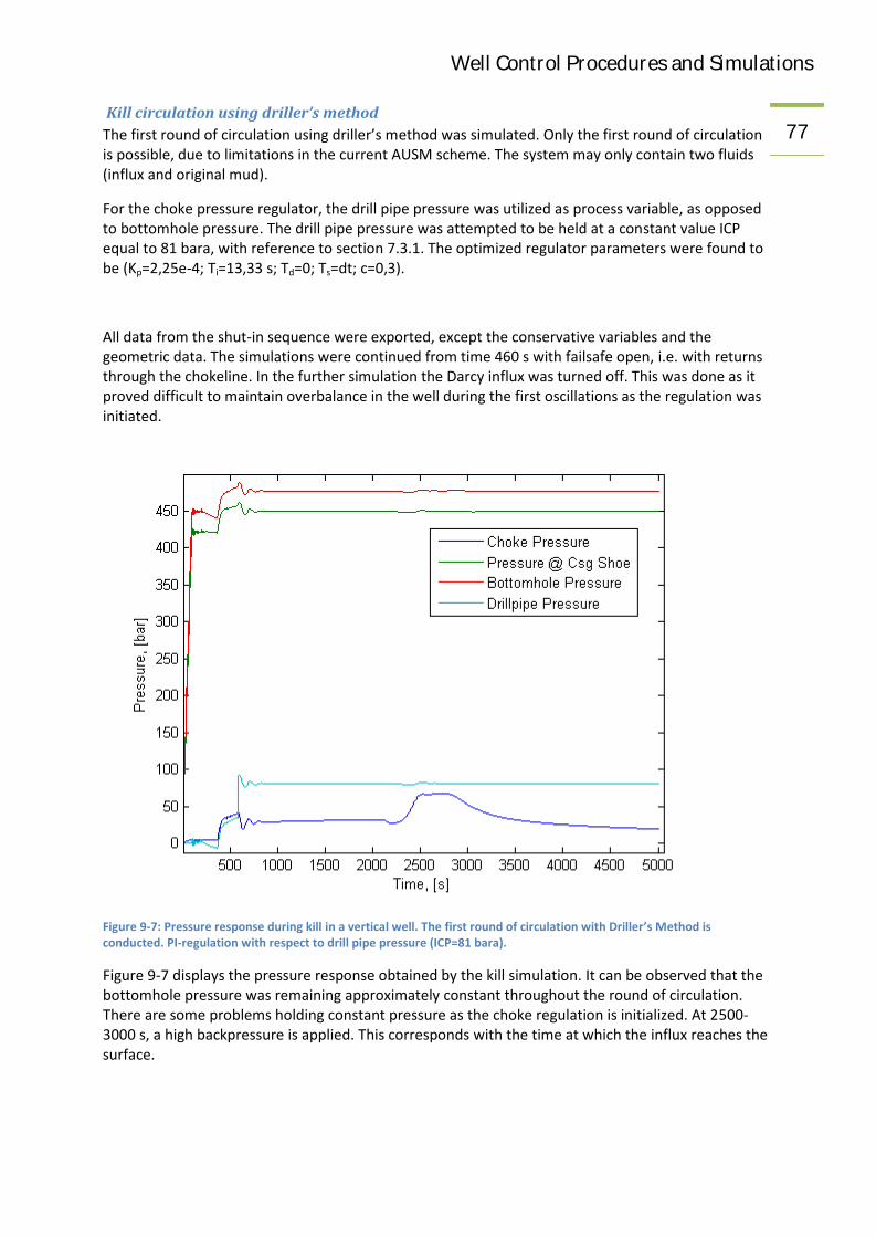
Well Control Procedures and Simulations77Kill circulation using driller’s method
The first round of circulation using driller’s method was simulated. Only the first round of circulationis possible, due to limitations in the current AUSM scheme. The system may only contain two fluids(influx and original mud).
For the choke pressure regulator, the drill pipe pressure was utilized as process variable, as opposedto bottomhole pressure. The drill pipe pressure was attempted to be held at a constant value ICPequal to 81 bara, with reference to section 7.3.1. The optimized regulator parameters were found tobe (Kp=2,25e-4; Ti=13,33 s; Td=0; Ts=dt; c=0,3).
All data from the shut-in sequence were exported, except the conservative variables and thegeometric data. The simulations were continued from time 460 s with failsafe open, i.e. with returnsthrough the chokeline. In the further simulation the Darcy influx was turned off. This was done as itproved difficult to maintain overbalance in the well during the first oscillations as the regulation wasinitiated.
Figure 9-7: Pressure response during kill in a vertical well. The first round of circulation with Driller’s Method isconducted. PI-regulation with respect to drill pipe pressure (ICP=81 bara).
Figure 9-7 displays the pressure response obtained by the kill simulation. It can be observed that thebottomhole pressure was remaining approximately constant throughout the round of circulation.There are some problems holding constant pressure as the choke regulation is initialized. At 2500-3000 s, a high backpressure is applied. This corresponds with the time at which the influx reaches thesurface.

Well Control Procedures and Simulations78Worst case simulations
First a gas filled well scenario was considered. The simulation was run until the entire well wasdisplaced to gas. Then the well was shut-in and the bottomhole pressure was allowed to increaseuntil it was equal with the formation pressure. Total simulation time was 20000 s.
Figure 9-8: Gas filled well scenario (approach #1) in a vertical well.
In Figure 9-8, a gas filled well scenario is simulated. It can be observed from the various pressuresthat the well is completely filled with gas at close to 4000 s. Steady state gas migration continuesuntil the well is shut-in at time 10000 s. A build up of pressure occurs until the bottomhole pressureequalizes the formation pressure around time 14000 s. The little separation between the bottomholepressure and the pressure at the casing shoe is caused by a small vertical displacement between thecasing shoe and bottomhole. The distance between the two points is only 150 m.
Another observation is that the drill pipe pressure has negative values due to the u-tube effect.Negative pressures are physically impossible, but the effect is caused by the drilling fluid beingmodeled as incompressible within the drillstring. Maximum and minimum pressures recorded at thecasing shoe is 467 bara and 46,4 bara.
Secondly an alternative approach was investigated. The concept is to take a kick, shut-in and let thegas migrate to the top. The data from the shut-in sequence were exported, and the simulationcontinued with failsafe open (see section 8.2.7). The well is shut-in at RKB. This will cause anoverestimation of the downhole pressures after gas break through. By assuming incompressibleliquid, the overestimation is approximated to the high side of 2 bar (liquid density · gravity · chokelinevolume/annular capacity).

Well Control Procedures and Simulations79
Figure 9-9: Alternative worst case scenario (approach #2). Gas migration in a shut in vertical well.
Figure 9-9 illustrates gas migration in a shut in well. At time less than ~500 s the shut-in sequence istaking place (see Figure 9-6). In the interval ~500-800 s a slightly different slope can be distinguishedfor the casing shoe pressure compared to the bottomhole pressure. This is due to gas contents in theannular volume below the casing shoe. From 800 to around 4000 s there is an approximately linearrise in downhole pressures. This is due to steady gas migration. Then the slope of the curvesdecreases. This is caused by gas break-through at surface. After 4000 s, there is still a raise indownhole pressures as gas accumulates below the choke manifold. The highest recorded pressure atthe casing shoe was 678 bara. Considering that the pressure is still increasing and the estimated errorof 2 bar, 678 bara seems like a generous estimate for the maximum pressure on the casing shoe.
9.2.2. Horizontal wellA horizontal well was initialized. The well is vertical to the kick off point situated at 2580 m RKB. Auniform build rate is used and from 3240 m MD and out the well is horizontal (90 deg inclination).Total well depth is 3840 m MD and 3008 m TVD. The 13 3/8 inch (ID = 32 cm) casing shoe is situatedat 3690 m MD, and the remaining 150 m consists of 12 ¼ inch open hole. Water depth is 210 m RKB,with 18 ¾ inch riser and 3 inch chokeline. The drillstring is composed of 5 inch drillpipe and a 90 m 8½ inch BHA. The capacity in the drillstring is assumed to be 8 l/m, uniform throughout the entiredrillstring (including BHA). The very same well is used in the example calculations in section 7.3.2.
For the simulations on the horizontal well the hydrostatic of the fluid column in the drillstring wasnot adjusted. Since the well is 8 m TVD deeper this results in an overestimation of the drillpipepressure 1,1-1,2 bar.

Well Control Procedures and Simulations80Simulated SCR
As for the vertical case, the SCR in the horizontal well was conducted at 600, 800 and 1000 lpm.
Figure 9-10: SCR through the riser in a horizontal well. The dynamic pressure loss is subdivided in to its respectivepressure loss components.
Figure 9-10 illustrates the recorded dynamic pressure loss through the riser during an SCR. Thedynamic pressure loss is subdivided into its respective pressure loss components. The SCR isconducted in a horizontal well.
An initial observation is that the dynamic pressure loss is higher for the horizontal well than for thevertical well. This is expected since the frictional pressure loss is depending on the measured depth.Further investigation shows that the increase in dynamic pressure loss is primarily due to increase indrillstring friction. The other components are nearly equal for the horizontal and the vertical well.
Dynamic pressure loss when circulating through the riser at 1000 lpm is measured to 64,68 bar, orusing field practice rounding rules 65 bar.
An SCR was also conducted through the chokeline. The plot is not included as it was very similar tothe previous plot and the plots in section 0. Compared to the previous plot, the main difference wasthe chokeline friction. When comparing with Figure 9-5, the primary difference is the increasedfrictional pressure loss in the drillstring.
The dynamic pressure loss when circulating at 1000 lpm through the chokeline is measured to 75,25bar, or using field practice rounding rules 76 bar.

Well Control Procedures and Simulations81Shut-in
A gas kick is taken from time 200 s in a horizontal well. A formation pressure of 475 bara is assumed.The reference mass rate is assumed to be 10 kg/s. The well is shut-in at time 370 s, and the influx willcontinue until the bottomhole pressure equals the formation pressure.
Figure 9-11: Shut-in in a horizontal well. Pit gain and actual influx volume refers to the secondary ordinate axis.
Figure 9-11 displays the shut-in sequence for a horizontal well. The influx of formation fluidscontinues until the well again is in overbalance. This occurs at time 570 s, and the shut-in pressuresand the pit gain is read. In the time following there is no increase in downhole or topside pressures,nor any increase in actual influx volume. This is caused by the implemented slip relation and theassumption of no slip in the horizontal section of the well.
The pit gain and the actual influx volume refer to the secondary ordinate axis. The actual influxvolume is obtained by a summation of the gas volumes in the lower segments. It can be observedthat the pit gain and the actual influx volume at shut-in are not equal. This is due to the well keepsflowing until the bottomhole pressure matches the formation pressure.
SIDPP, [bar] SICP, [bar] Pit gain, [m3] Influx volume,[m3]
Influx mass, [kg]
25,1 27,6 3,46 3,74 1773Table 9-2: Various values read at shut-in in the horizontal well. The influx volume and influx mass are the actualdownhole values obtained by summing gas volume and mass for the bottom segments.

Well Control Procedures and Simulations82
The three first values in Table 9-2 are the top side pressure and volume values at shut-in. These arethe values used in the example calculations in the analytical model (section 7.3.1). The influx volumeand mass refers to actual downhole values at shut-in. They are obtained by a summation of the gasvolumes and masses in the lowermost segments. The reason for a difference in pit gain and actualinflux volume is the expansion of the influx continues after the well has been shut-in.
Kill circulation using driller’s methodA kick is circulated out using Driller’s Method in a horizontal well. The regulator parameters weretuned to (Kp=33,75e-4; Ti=47,5 s; Td=0; Ts=dt; c=0,6). The regulation was done with the drillpipepressure functioning as a process variable. Due to a mishap, the set pressure (ICP) was set to 93 bara,while the calculated value was 91 bara. It is assumed that simply subtracting 2 bar off of all downholepressure will not cause any significant errors.
Similarly as for the vertical case the shut-in sequence was continued with the riser closed and thechokeline open.
Figure 9-12: Pressure response during kill in a horizontal well. The first round of circulation with Driller’s Method isconducted. PI-regulation with respect to drill pipe pressure (ICP=93 bara). The casing shoe pressure is coinciding with thebottomhole pressure due to no vertical displacement.
Figure 9-12 illustrates the pressure response in the horizontal well as a kick is circulated to surface. Itcan be observed that the casing shoe pressure coincides with the bottomhole pressure. This iscaused by no vertical displacement between the two points. It is also evident that the time tocirculate the kick to surface is remarkably longer than for the vertical case. This is partly due to anincreased measured depth, partly due to low drift velocities in the deviated sections. Another

Well Control Procedures and Simulations83observation is the smoothness of the curves corresponding to the downhole pressures and the choke
pressure. An explanation may be suggested with reference to the sensitivity testing of section 8.2.4.Due to the increase in measured depth (compared to section 0), the influx will be more distributed asit reaches the surface. This results in low volumetric rates of gas across the choke and hence, betterregulation.
Worst caseThere was conducted a simulation on the gas filled well scenario. However, it was decided to leave itout from the thesis as is displayed the exact same results as for the vertical case (within 1 bar). Thealternative worst case scenario was not simulated, as the implemented slip relation will cause no gasmigration in the horizontal section.
Well Control Procedures and Simulations84
10. Discussion and analysisIn this section the development of the simple kick simulator will be discussed. Further, the resultsobtained from the well control simulations will be analyzed and compared with the calculated datafrom the analytical model.
10.1. On the development of a crude kick simulatorA simple kick simulator has been developed with basis in the numerical AUSMV scheme. The purposewas to realistically model well control simulations, and to compare analytical results with thesimulated results obtained by use of the numerical scheme. The primary objective was to verify orexpose weaknesses in the traditional well control calculations.
10.1.1. Benefits and possibilities by utilizing a numerical schemeThere are several advantages using a numerical scheme compared to the simple kill sheet. Whenusing the proposed model, a variety of complex physical effects can be treated in a fairly realisticmanner.
Pressure pulsesThe AUSMV scheme can be used to handle propagating sonic waves in two-phase mixtures. In a killsheet, pressure pulses are completely neglected. It has been shown that a rapid increase in pressureproduces excessive oscillations and water-hammering in one-phase liquid. The effect is exponentiallydampened by friction. In two-phase mixtures with high volume fractions of gas, the effect is not aspronounced. This is reasonable, as the water-hammering will be partially absorbed by thecompressible gas. It has also been shown that the speed of sound in a two-phase mixture is lowerthan in one-phase liquid or gas.
The numerical schemes have applications in well control training simulators, where the time delaybetween an adjustment in applied backpressure or pump rate will propagate with the speed ofsound of the two-phase mixture.
Frictional effectsKill sheets and simple analytical models utilize simplifying assumptions when it comes to frictionalpressure loss. In the numerical scheme, the friction can be modeled more realistically byimplementation of experimental or analytical friction models. Hence, the numerical scheme can beused to test the validity of the assumptions made in the analytical model.

Well Control Procedures and Simulations85Gas slippage
In a kill sheet, the influx is modeled as single bubble. An influx is assumed to propagate with no slipcompared to the liquid fraction, or at a constant drift velocity. However, due to gas slippagedepending on gravity and flow regime the influx will be distributed. This causes the analytical modelsto be more conservative than the numerical schemes. Drilled kicks will be additionally distributed, asthey are taken with the pumps running. Connection kicks or swabbed kicks may be moreconcentrated. Another effect caused by gas slippage, is that gas breakthrough at RKB level occursahead of time according to the calculated time to circulate bottoms up.
Figure 10-1: Gas distribution and migration in a shut in vertical well. Segment 1 refers to bottomhole, segment 50 totopside. The plot is produced in conjunction with Figure 9-9.
Figure 10-1 illustrates the gas distribution profiles in a shut-in wellbore at various points in time. Thewell is vertical, and the displacement of the gas volume is caused by gas migration. It can also beseen that the area below the distribution profiles is approximately constant. Hence, the pressure inthe gas will be fairly constant at the different points in time.
CompressibilityThe traditional analytical model assumes incompressible liquid. Using the numerical scheme, anincrease in average static density in the order of magnitude of a couple of points compared to thedensity at standard conditions, was obtained for a well of 3000 m TVD. Both the liquid and gas

Well Control Procedures and Simulations86compressibilities are overestimated in the current numerical schemes. This is caused by
unrealistically low sonic velocities in the one-phase fluids.
Under realistic conditions the compressibility effects will be counteracted by temperature effects.The current numerical scheme does not take into account temperature variations.
Figure 10-2: Liquid densities at different points in time in a shut in vertical well. The overall pressure is increasing as afunction of time. The segments are numbered from bottomhole and upwards. The plot is produced in conjunction withFigure 9-9.
Figure 10-2 displays the compressible nature of a drilling fluid. The liquid density increases as afunction of the prevailing pressure conditions in the wellbore. The plot is produced as a volume ofgas migrates in a shut-in vertical well.
10.1.2. PI-regulationWhen a conventional kill method is applied in order to circulate a kick out, the bottomhole pressureis held steady at a constant value in slight overbalance against the formation pressure. The AUSMVscheme does not allow for setting the bottomhole pressure constant. This is due to the accelerationterms of the drift flux model. Thus, there was a need to implement a method with the ability to keepthe bottomhole pressure stable within a reasonable interval.
A simple PI-regulator was implemented. It functions by regulating the choke pressure directlywithout the use of a choke model. Both drillpipe pressure and bottomhole pressure was regulatedsuccessfully. However, the regulation required comprehensive tuning and adjustment in order tofunction satisfactory.

Well Control Procedures and Simulations87The sensitivity of the PI-regulator was tested with respect to changes in well dynamics. It was initially
assumed that the rate of convergence and the stability of the PI-regulator would increase as an effectof a reduction in system dynamics. The assumption was supported by two sets of tests with variablewell depth and influx mass. However during a third set of tests with variable kill rate, it wasdiscovered that the stability of the regulation was reduced at reduced pump rates. This is incontradiction to the initial assumption, and should be further investigated.
A slightly new approach for PI-regulation was discovered, which displayed impressive properties andperformance with respect to stable and convergent regulation. The reasons for the success are notfully understood, but it seems to capture the dynamic nature of a kill in a better manner than what isthe case for the conventional approach. The new approach was used in all the conducted killsimulations.
10.1.3. Additional modifications and extensions to the numerical schemeThe PI-regulation of the bottomhole pressure was the most important and time consuming extensionin order to adapt the numerical scheme to application in well control scenarios. Additionally, variousminor modifications were conducted in order to increase the realism and suitability of the scheme asa simple kick simulator.
The ability to read well control parameters such as drillpipe pressure and pit gain was implemented.This was done for the ability to compare the simulated results with the kill sheet calculations.Further, a simple chokeline and riser was incorporated, for the purpose of simulations on subseawells. Additional modifications were made in order to conduct simulations on deviated andhorizontal wells.
More realistic friction models were tested and implemented, amongst others to model turbulentflow with a high degree of accuracy. The density of the liquid component in the system was changedto resemble a typical drilling fluid. In addition, a pressure dependent influx function wasimplemented. Hence, the shut-in sequence can be modeled more accurately. Initially, thebottomhole pressure and the choke pressure were measured in the midpoint of the bottom and topsegment. For a 3000 m well with 50 segments, this cause an error in the read pressure of around 4bar at static conditions (1,5 SG mud). This was altered by extrapolation, such that the pressures areactually measured at the end points.
A choke model was implemented, but not used in the simulations.

Well Control Procedures and Simulations8810.2. Interpretation of the well control simulations in light of the
analytical modelWell control simulations have been conducted on a vertical and a horizontal well. The results fromthe simulations will be discussed and compared to corresponding values obtained from the analyticalmodel.
10.2.1. Kick simulations using driller’s methodIn the vertical case the average bottomhole pressure overbalance throughout the round ofcirculation is 2,1 bar. The corresponding overbalance in the deviated well is 1,2 bar (subtracted the 2bar excess ICP, see section 9.2.2). Further analysis is required in order to find the reason for theoverbalance.
ICP calculationIn a kill situation, it is often assumed that the pressure losses in the annulus and riser are negligible,due to a relatively high cross sectional area and low liquid velocities. This causes the initial circulatingpressure to be calculated as the sum of the dynamic pressure loss and the shut-in drillpipe pressure.
Analysis is conducted on the horizontal well as this will produce higher frictional pressure loss in theannulus. Thus, the error by assuming negligible annular friction is greater.
Figure 10-3: Plot obtained from the SCR for the deviated well. Due to a problem with obtaining consistent pressures, thevalues have been parallel displaced in such a way that the pressures losses are zero at zero flow rate. The kill sheetestimate refers to the simulated dynamic pressure loss through the riser, which is used directly when calculating the

Well Control Procedures and Simulations89initial circulating pressure. The simulated pressure loss in the drillstring is the sum of the pressure loss across the bit and
the friction in the drillstring.
Figure 10-3 illustrates the difference between the estimated drillstring pressure loss (dynamicpressure loss through the riser) and the actual pressure loss through the drillstring (sum of thedrillstring friction loss and the pressure loss across the bit). It is evident that the values coincide to ahigh degree. Another observation is that the difference between the estimated and the true valuesseems to increase at higher flow rates. The difference between the estimate and the actual losscomponents at kill rate (1000 lpm) is 0,5 bar (see Table 10-1 for elaboration). This may serve as asafety margin.
Flow Rate, [lpm] Kill Sheet Estimate,[bar]
Simulated PressureLoss in Drillstring,
[bar]
Safety Margin
600 24,6 24,6 0800 41,7 41,2 0,51000 62,9 62,2 0,5Table 10-1: Values obtained from Figure 10-3. The kill sheet estimate is the corrected dynamic pressure loss through theriser. This is used directly when calculating the initial circulating pressure. The simulated pressure loss in the drillstring isthe sum of drillstring friction and pressure loss across the bit. The safety margin is obtained by subtracting the simulatedpressure loss in the drillstring from the kill sheet estimate. This value reflects the associated downhole overbalanceproduced by applying a choke pressure equal to shut-in casing pressure subtracted the kill sheet estimate of thechokeline friction (relevant in when initiating a kill circulation).
The field practice rounding rules will add an additional safety margin towards the formation pressureof 0,8 bar (dynamic pressure loss is rounded up to the nearest integer bar). This yields a total safetymargin of 1,3 bar caused by the ICP. It is noticed that the safety margin produced by the ICP is 0,1 barhigher than the average bottomhole overbalance.
FCP calculationThe calculation of the final circulating pressure relies on a direct proportionality between thedynamic pressure loss measured through the riser and the liquid density (see equations (7.10) and(7.14)). In this section the proportionality will be further investigated. The final circulating pressure ishowever not included in the simulations, due to limitations in the numerical scheme.
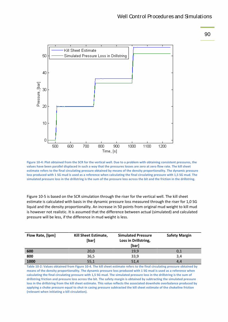
Well Control Procedures and Simulations90
Figure 10-4: Plot obtained from the SCR for the vertical well. Due to a problem with obtaining consistent pressures, thevalues have been parallel displaced in such a way that the pressures losses are zero at zero flow rate. The kill sheetestimate refers to the final circulating pressure obtained by means of the density proportionality. The dynamic pressureloss produced with 1 SG mud is used as a reference when calculating the final circulating pressure with 1,5 SG mud. Thesimulated pressure loss in the drillstring is the sum of the pressure loss across the bit and the friction in the drillstring.
Figure 10-5 is based on the SCR simulation through the riser for the vertical well. The kill sheetestimate is calculated with basis in the dynamic pressure loss measured through the riser for 1,0 SGliquid and the density proportionality. An increase in 50 points from original mud weight to kill mudis however not realistic. It is assumed that the difference between actual (simulated) and calculatedpressure will be less, if the difference in mud weight is less.
Flow Rate, [lpm] Kill Sheet Estimate,[bar]
Simulated PressureLoss in Drillstring,
[bar]
Safety Margin
600 20,0 19,9 0,1800 36,5 33,9 3,41000 55,1 51,4 4,4Table 10-2: Values obtained from Figure 10-4. The kill sheet estimate refers to the final circulating pressure obtained bymeans of the density proportionality. The dynamic pressure loss produced with 1 SG mud is used as a reference whencalculating the final circulating pressure with 1,5 SG mud. The simulated pressure loss in the drillstring is the sum ofdrillstring friction and pressure loss across the bit. The safety margin is obtained by subtracting the simulated pressureloss in the drillstring from the kill sheet estimate. This value reflects the associated downhole overbalance produced byapplying a choke pressure equal to shut-in casing pressure subtracted the kill sheet estimate of the chokeline friction(relevant when initiating a kill circulation).

Well Control Procedures and Simulations91Table 10-2 displays the values obtained from Figure 10-4. It is observed that the safety margin
produced by applying the final circulating pressure on the drillstring side increases as a function ofpump rate. The field practice rounding rules provides an additional margin towards the formationpressure.
Estimation of chokeline frictionChokeline friction is often used as a means for initiating a kill circulation. When circulation isinitiated, the pump output is gradually brought to kill rate, while the choke valve is slowly opened. Atkill rate it is often assumed that the choke pressure corresponding to constant bottomhole pressure,equals shut-in pressure subtracted the chokeline friction (see equation (7.12)). Chokeline friction isthen calculated from the measured dynamic pressure losses as described in the equation.
Figure 10-5: Plot obtained from the SCR for the horizontal well. Due to a problem with obtaining consistent pressures,the values have been parallel displaced in such a way that the pressures losses are zero at zero flow rate. The kill sheetestimate refers to a value for chokeline friction obtained by subtracting the simulated dynamic pressure loss through theriser from the simulated dynamic pressure loss through the chokeline. The simulated chokeline friction is the frictioncomponent obtained directly from the simulation. Simulated friction on annulus side is obtained by adding the frictionalcomponents on the annulus side (simulated annular friction added simulated chokeline friction).
Figure 10-5 is produced with basis in the SCRs conducted in the horizontal well (section 9.2.2). It isevident that the estimated chokeline friction slightly overestimates the simulated chokeline friction.However, what is interesting in context of keeping the well in overbalance, is actually the entirepressure loss on the annulus side. The estimated chokeline friction underestimates the pressure losson the annulus side. Hence, this yields a positive safety margin bottomhole.

Well Control Procedures and Simulations92Flow rate, [lpm] Kill Sheet Estimate,
[bar]Simulated
Chokeline Friction,[bar]
Simulated Frictionon Annulus Side,
[bar]
Safety Margin,[bar]
600 3,6 3,6 4,0 0,4800 6,2 6,1 6,6 0,41000 9,3 9,2 9,9 0,6Table 10-3: Values obtained from Figure 10-5. The safety margin is obtained by subtracting the simulated friction onannulus side from the kill sheet estimate. This value reflects the associated downhole overbalance produced by applyinga choke pressure equal to shut-in casing pressure subtracted the kill sheet estimate of the chokeline friction (relevant inwhen initiating a kill circulation).
In Table 10-3 the values from the previous figure is posted. It is observed that the safety margin at killrate is 0,6 bar. The field practice rounding rules will decrease the safety margin. However, therelation for establishing circulation is only used as a guideline. In an actual kill situation, the drillpipepressure will be utilized for determining the applied choke backpressure.
Estimation of influx sizeThe measured pit gain at surface is an estimate of the influx size. However, it is not a good estimate,as the formation will keep flowing in some time after the well is shut-in. The influx volume will alsochange as it propagates towards the surface, and as will the influx density. The only obtainableinvariant value reflecting a kick size is its mass.
Vertical Well Horizontal WellKill Sheet Simulated Kill Sheet Simulated
Volume, [l] 4330 4640 3460 3740Density, [SG] 1,0 0,45 N/A 0,47Mass, [kg] 4330 2082 N/A 1773Table 10-4: Influx size as determined directly from shut-in simulations in sections 9.2.1 and 9.2.2, and from the kill sheetcalculations in sections 7.3.1 and 7.3.2. The kill sheet volumes which are referred to, is the pit gain measured at shut-in.
In Table 10-4 values reflecting the kick size is posted. The kill sheet values are values calculated insections 7.3.1 and 7.3.2, for the vertical well and horizontal well respectively. The volume in the killsheet column is the measured pit gain. The simulated values are obtained directly from the shut-insequences of sections 9.2.1 and 9.2.2.
An initial observation is that there is no kill sheet values for density or mass obtained for thehorizontal well. This is due to zero vertical influx height. Hence, equation (7.19) is meaningless.Another observation is the major discrepancy between calculated values and simulated values formass and density in the vertical well. The reasons for this are not understood, and should beinvestigated.
Estimation of formation pressureIn both the vertical and the horizontal well control simulations, the formation pressure was set to475 bara. However, when calculating the formation pressure from the kick data using equation(7.15), the calculated pressure was an average of 5,5 lower than the actual 475 bara. This isinterpreted as an effect of the compressible mud. Since the average density of the drilling fluid inreality is higher than the density at standard conditions, incompressible mud yields a slightunderestimation of the formation pressure.

Well Control Procedures and Simulations93The underestimation of the formation pressure will cause a successive underestimation of the kill
mud density. However, this is assumed to again be balanced by the increase in kill mud density dueto compressibility.
10.2.2. Worst case scenarios for well design purposesA gas filled well is commonly defined as a worst case scenario in well design. If the wellbore canwithstand the pressures exerted by the gas filled well scenario, it is said to have full well integrity.However, from Figure 9-8 and Figure 9-9 it can be observed that a gas bubble migrating in a shut-inwellbore result in higher downhole pressures than the conventional gas filled well scenario. Themaximum recorded pressure at the casing seat for the gas filled well scenario was 467 bara, whilethe shut-in gas migration caused an estimated casing shoe pressure of 678 bara (only estimation dueto shortage of data). This underlines that even though a wellbore is said to have full well integrity, itis still of great importance that the weakpoint of a wellbore is situated in the open hole section.

Well Control Procedures and Simulations94
11. ConclusionA crude kick simulator has been developed with basis in the drift flux model and the explicitnumerical scheme AUSMV. A range of modifications and extensions to the simple numerical schemehas been introduced.
When killing a kicking well, the bottomhole pressure is traditionally kept constant and in slightoverbalance compared to the formation pressure. The intention is to avoid further influx offormation fluids. This is achieved by applying a variable choke backpressure. The choke valve isoperated by rig personnel. As the AUSMV scheme does not allow for the bottomhole pressure simplyto be set to a constant value, the primary accomplishment in the development of the simple kicksimulator was the implementation of an automatic PI-regulator. The PI-regulator keeps thebottomhole pressure constant within reasonable limits, as an influx is circulated out from thewellbore. Extensive tuning is required each time the dynamics or the geometry of the well is altered.
The sensitivity of the regulator was tested with respect to variable system dynamics (well depth,influx size and kill rate). It was assumed that the stability and rate of convergence of the regulatorwould improve as a function of reduced dynamics. However, unexpected instability was experiencedat low kill rates. The reasons for this are not understood, and should be further investigated.
A novel approach to the pressure regulation was discovered. The approach takes advantage of theclassical equation defining the PI-regulator, and introduces an additional variable which reflects thedynamic state of the wellbore system. The approach has shown admirable results compared to theclassical PI-regulator. The reasons for the success are however not fully understood, and should beinvestigated more extensively.
The additional modifications and extensions with respect to the numerical scheme can be summedup as follows,
A more realistic friction model. Chokeline and riser for simulation on subsea wells. Implementation of a possibility for wellbore deviation. A more accurate reading of bottomhole and casing pressures. A drillstring function, which makes it possible to read drillpipe pressure. A pit gain reading. A Darcy relation for influx where influx size and mass rate depends on downhole pressure
differential. This is important for simulations on drilled kicks or connection kicks. Changing the liquid component of the system from water to drilling fluid (altering the liquid
density). Additionally, a choke model was implemented in the model, but it has not been used in the
simulations. The choke model depicts the backpressure as a function of fluid density, flowrate and choke opening.

Well Control Procedures and Simulations95The developed kick simulator was used for well control simulations in one vertical and one horizontal
well. The simulated data was compared with results from corresponding well control formulas. It wasfound that even though the estimates obtained from the formulas and kill sheets were not alwayscorresponding with the simulated results, the errors produced by the formulas exclusively wouldfunction as safety margins with respect to the downhole pressure overbalance. Although thetraditional well control formulas rely on a range of simplifying assumptions, they have proved toperform surprisingly well during the conducted well control simulations.
A major discrepancy was found when calculating the influx density and the influx mass from the shut-in pressures and the pit gain for the vertical well. Both of the calculated values were around twicethe magnitude of the values obtained directly from the simulation. The cause of this is not known.
Simulations on well control scenarios indicated that the conventional gas filled well scenario inducesless pressure at the weakpoint than a gas bubble migrating in a shut-in annulus. It is thereforeimportant to ensure that the weakpoint of a wellbore is located in the open hole section, even if thewell is said to have full well integrity.
11.1. Further workThe AUSMV scheme has potential as a kick simulator. If simulations similar to the ones presented inthis thesis are to be conducted, it is recommended to model the drillstring in a better manner. Byalso using the AUSMV scheme within the drillstring, one could obtain more accurate simulationresults. Particularly compressibility is important for trustworthy readings of drillpipe pressure.Further, it is suggested to implement an ability to shut-in the well at seabed, and to take returnsthrough the chokeline or riser as desired. This would add flexibility to the simulations and open newpossibilities for modeling for instance hard and soft shut-in. Another recommendation is to makebetter use of the implemented choke model.
Two issues should be resolved. The underestimation of fluid velocities at low flow rates causesinaccuracy, primarily with respect to friction loss. It has been shown that the error is reduced at finerdiscretization. However, it should be investigated if this malfunction could be resolved completely.The second issue is the PI-regulator. The tuning of the regulator is quite cumbersome and timeconsuming. A better way to maintain constant bottomhole pressure should be established. If thiscannot be achieved, perhaps the biggest potential in the current scheme is as a training simulator,where the bottomhole pressure does not need to be automatically regulated.
Well Control Procedures and Simulations96
References1. Standard Norway, NORSOK STANDARD D-010: Well integrity in drillingand well operations. 2004.2. American Petroleum, I., Recommended practice for well controloperations: upstream segment. 2006, Washington, D.C.: API. V, 92 s.3. Transocean, Well Control Handbook. 3rd ed. 2009.4. Mitchell, R.F., Drilling engineering. Petroleum engineering handbook.Vol. Vol. 2. 2006, Richardson, Tex.: Society of Petroleum Engineers.viii, 763 s.5. Aadnøy, B.S., Modern well design. 2010, Boca Raton: CRCPress/Balkema. X, 303 s.6. Fjelde, K.K., SVALEX Festningen Pt. 3 (unpublished). 2010: Stavanger.7. American Petroleum, I., Specification for casing and tubing: APISpecification 5CT, Eight ed., July 1, 2005 = ISO 11960:2004, Petroleumand natural gas industries - steel pipes for use as casing and tubing forwells. 2005, Washington, D.C.: American Petroleum Institute. 291 s.8. Gabolde, G. and J.-P. Nguyen, Drilling data handbook. 2006, Paris:Editions Technip. 1 b. (flere pag.).9. Garnier, A.J. and N.H.v. Lingen, Phenomena Affecting Drilling Rates atDepth. 1959.10. Jorden, J.R. and O.J. Shirley, Application of Drilling Performance Datato Overpressure Detection. SPE Journal of Petroleum Technology,1966. 18(11).11. Standard Norway, NORSOK STANDARD D-001: Drilling facilities. 1998.12. Finnemore, E.J., J.B. Franzini, and R.L. Daugherty, Fluid mechanics withengineering applications. 2002, Boston: McGraw-Hill. XXV, 790 s.13. Watson, D., T. Brittenham, and P.L. Moore, Advanced well control. SPEtextbook series. Vol. vol. 10. 2003, Richardson, TX: Society ofPetroleum Engineers. IX, 386 s.14. Shi, H., et al., Drift-Flux Modeling of Multiphase Flow in Wellbores, inSPE Annual Technical Conference and Exhibition. 2003: Denver,Colorado.15. Liou, M.-S. and C.J. Steffen, A New Flux Splitting Scheme. Journal ofComputational Physics, 1993. 107(1): p. 23-39.16. Wada, Y. and M.-S. Liou, An Accurate and Robust Flux Splitting Schemefor Shock and Contact Discontinuities. SIAM J. Sci. Comput., 1997.18(3): p. 633-657.17. Evje, S. and K.K. Fjelde, Hybrid Flux-Splitting Schemes for a Two-PhaseFlow Model. Journal of Computational Physics, 2002. 175(2): p. 674-701.

Well Control Procedures and Simulations9718. Fjelde, K.K., Evje, S., The AUSMV Scheme - A Simple but Robust Model
for Analyzing Two-Phase Flow (unpublished work note). 2010,University of Stavanger: Stavanger.19. LeVeque, R.J., Finite volume methods for hyperbolic problems. 2002,Cambridge: Cambridge University Press. XIX, 558 s.20. Lage, A.C.V.M., Two-phase flow models and experiments for low-headand underbalanced drilling. 2000, UiS: [Stavanger]. p. XXIV, 218 s.21. Haugen, F., Praktisk reguleringsteknikk. 2003, Trondheim: Tapirakademisk forl. 278 s.

Well Control Procedures and Simulations98
A. Appendix
A.1. Closed circuit Ziegler-Nichols routineThe routine used for tuning the choke regulators used in this thesis, is based on Ziegler-Nichols routine for closed circuits. As a means for reproducing the results obtained in thisthesis, this detailed routine is presented.
Kp Ti Td
P-regulator
0,5*Kpk Infinity 0
PI-regulator
0,45*Kpk Tp/1,2 0
PID-regulator
0,6*Kpk Tp/2 Tp/8
Table A-1: Table for calculation of tuning parameters.
1. Set Ti to 10 000 000 and Td to 0, so that the output produced from the integral termand the derivate term of the PID-regulator is zero. Thus, the regulator is reduced to aP-regulator.
2. Ts is set equal to dt, or a positive multiple of dt, depending on the desired frequency ofregulation.
3. Set Ki to a low value (0,1 has been used), and run a simulation. The simulation iseither run with a rapid increase in pump rate, or with a propagating kick in thewellbore, in order to provoke instability in the system.
4. Increase the value of Kp in steps of 0,1 until sustained oscillations occur.5. The critical proportional gain Kpk, is defined as the lowest value of Kp which produces
sustained oscillations. It is read with one decimal. A tuned Kp value is set according tothe table. The Kp value is set to three decimals.
6. The critical period Td, is defined as the period of the oscillations produced by the PID-regulator with proportional gain equal to critical gain. The Td value is read as aninteger (whole seconds). Tuned values for Td and Ti are set according to the table. Thetuned values are rounded to two decimals.
7. In general, the regulator used is a PI-regulator, where Td is set to zero.8. If desired, rate of convergence or stability may be improved by scaling the regulator
parameters. This is done by multiplying Kp, 1/Ti and Td with a common factor, c.Thus, the proportional term is multiplied with c, and the integral and derivative termsare multiplied with c2.

Well Control Procedures and Simulations99
A.2. Matlab CodeThe complete Matlab code is included in the following sections.
main.m%% Transient AUSMV scheme
clear;
% Geometry data/ Must be specifiedwelldepthmd = 3000;nobox = 25;% nobox = 64;nofluxes = nobox+1;dx = welldepthmd/nobox; % Bokslengde% dt= 0.0125; % Tidsteg må reguleres i forhold til valgt bokslenge ogCFL krav.dt= 0.025;dtdx = dt/dx;time = 0;endtime = 1200; % Lengde på simulering i sekundnosteps = (endtime-time)/dt;timebetweensavingtimedata = 5;nostepsbeforesavingtimedata = timebetweensavingtimedata/dt;
% Slip parameters of gas/can be adjusted vg = Kxvmix+s for vertical,% assume no-slip for horizontal. vg=((k-1)cos(ang)+1)xvmix+scos(ang)k = 1.2;s = 0.5;% k=1; %No-slip% s=0; %No-slip
% Viscosities (Pa*s)viscl = 0.05;viscg = 0.000005;
% Density parameters
% liquid density at stc and speed of sound in liquid. Viss vi skal inn% med en mud i stedet for vann må vi endre her.
dstc = 1500.0;pstc = 100000.0;al = 1000;t1 = dstc-pstc/(al*al);
% Ideal gas law constantrt = 100000;
% Gravity accelerationgrav = 9.81;
% Kick schedule (on/off)kickschedule=0;

Well Control Procedures and Simulations100% SCR schedule (on/off)
SCRschedule=0;
% BOP Well status (open = 1, closed = 0). BOP is situated at surface.bop = 0;
% Choke status (open = 1, closed = 0)choke = 1;
% High resolution recorder [on/off, start time, stop time]hrrecord= [0, 0,570];
% Fricion recorder (on/off)frictionrecord=0;
% Pit gain [on/off, start time]influxrecord=[0,200];
%Choke regulator (on/off)regulator=0;
% Geometry of circulation system. Lengths given in number of segments.The% change in cross-section occurs at the segment midpoint below.
waterdepth=4;%-1/2 Length of chokeline and riserbhalength=2; %-1/2 Length of BHAohlength=3; %-1/2 Length of open holekop=22; %kick off point below segment #kopeob=10; %end of build above segment #eobbhinclination=0*pi()/2; %inclination measured in rad in the lower
segments
% Failsafe status (open = 1, closed = 0)failsafe = 0; % Velger om sirkulasjon foregår gjennom chokeline(1)
eller riser(0). Kan ikkje opererast etter at simuleringa erinitialisert.
if failsafe == 0for i = nobox-waterdepth+1:nobox % DP x Riserdo(i) = 0.476; % 18 3/4"di(i) = 0.127; % 5"areal(i+1) = 3.14/4*(do(i)*do(i)- di(i)*di(i));arear(i) = 3.14/4*(do(i)*do(i)- di(i)*di(i));area(i) = 3.14/4*(do(i)*do(i)- di(i)*di(i));
endelseif failsafe == 1for i = nobox-waterdepth+1:nobox % Chokelinedo(i) = 0.0762; % 3"di(i) = 0.0;areal(i+1) = 3.14/4*(do(i)*do(i)- di(i)*di(i));arear(i) = 3.14/4*(do(i)*do(i)- di(i)*di(i));area(i) = 3.14/4*(do(i)*do(i)- di(i)*di(i));
endendfor i = max(bhalength,ohlength)+1:nobox-waterdepth % DP x Cased hole

Well Control Procedures and Simulations101do(i) = 0.32; % 13 3/8" OD - 2*wall thickness
di(i) = 0.127; % 5"areal(i+1) = 3.14/4*(do(i)*do(i)- di(i)*di(i));arear(i) = 3.14/4*(do(i)*do(i)- di(i)*di(i));area(i) = 3.14/4*(do(i)*do(i)- di(i)*di(i));
endfor i=bhalength+1:ohlength % DP x Open holedo(i) = 0.311; % 12 1/4"di(i) = 0.127; % 5"areal(i+1) = 3.14/4*(do(i)*do(i)- di(i)*di(i));arear(i) = 3.14/4*(do(i)*do(i)- di(i)*di(i));area(i) = 3.14/4*(do(i)*do(i)- di(i)*di(i));
endfor i=ohlength+1:bhalength % BHA x Cased holedo(i) = 0.32; % 13 3/8" OD - 2*wall thicknessdi(i)=0.2159; % 8 1/2"areal(i+1) = 3.14/4*(do(1)*do(1)- di(1)*di(1));arear(i) = 3.14/4*(do(1)*do(1)- di(1)*di(1));area(i) = 3.14/4*(do(i)*do(i)- di(i)*di(i));
endfor i=1:min(bhalength,ohlength) % BHA x Open holedo(i)=0.311; % 12 1/4"di(i)=0.2159; % 8 1/2"areal(i+1) = 3.14/4*(do(1)*do(1)- di(1)*di(1));arear(i) = 3.14/4*(do(1)*do(1)- di(1)*di(1));area(i) = 3.14/4*(do(i)*do(i)- di(i)*di(i));
endareal(1)=arear(1);areal (nobox+1)=[];welldepthtvd=0;
% load hzpf475t570shutindata.mat;
do(1:nobox)=0.1;di(1:nobox)=0;areal(1:nobox)=pi()/4*do.*do;arear(1:nobox)=areal(1:nobox);area(1:nobox)=areal(1:nobox);
for i = 1:noboxif i<=eob
ang(i)=bhinclination;elseif i>eob && i<kop
ang(i)=bhinclination*(1-(i-eob)/(kop-eob));else
ang(i)=0;endwelldepthtvd=welldepthtvd+dx*cos(ang(i));dl(i) = dstc;dlo(i)= dl(i);dg(i)= 1.0;dgo(i)=dg(i);vl(i) = 0.0;vlo(i)= 0.0;vg(i)= 0.0;vgo(i)= 0.0;p(i) = 100000.0;po(i) = p(i);eg(i)= 1.0;

Well Control Procedures and Simulations102ego(i)=eg(i);
ev(i)=1-eg(i);evo(i)=ev(i);
vg(i)=0.0;vgo(i)=0.0;vl(i)=0.0;vlo(i)=0.0;
vgr(i)=0.0;vgor(i)= 0.0;vgl(i)= 0.0;vgol(i)= 0.0;
vlr(i)=0.0;vlor(i)=0.0;vll(i)=0.0;vlol(i)=0.0;
qv(i,1)=dl(i)*ev(i)*(areal(i)+arear(i))*0.5;qvo(i,1)=qv(i,1);
qv(i,2)=dg(i)*eg(i)*(areal(i)+arear(i))*0.5;qvo(i,2)=qv(i,2);
qv(i,3)=(qv(i,1)*vl(i)+qv(i,2)*vg(i))*(areal(i)+arear(i))*0.5;qvo(i,3)=qv(i,3);
end
% Intialize fluxes
for i = 1:nofluxesfor j =1:3flc(i,j)=0.0;fgc(i,j)=0.0;fp(i,j)= 0.0;end
end
% Main program. Here we will progress in time. First somintializationshrcounter=1; % Refererer til high resolution pressure recorder.chokecounter=0; % Refererer til choke regulator;int=0; % Refererer til choke regulator.deriv=0; % Refererer til choke regulator.eo=0; % Refererer til choke regulator.countsteps = 0;counter=0;printcounter = 1;pressureoutlet=pstc;inletliqmassrate=0;inletgasmassrate=0;pdp(printcounter)=pstc;pbot(printcounter) = pstc;pchoke(printcounter)= p(nobox)+(p(nobox)-p(nobox-1))/2;

Well Control Procedures and Simulations103if
ohlength>0&&ohlength<nobox,pshoe(printcounter)=(p(ohlength)+p(ohlength+1))/2;end % Linear interpolation.if waterdepth>0,pseabed(printcounter) = (p(nobox-waterdepth)+p(nobox-waterdepth+1))/2;end % Linear interpolation.liquidmassrateout(printcounter) = 0;gasmassrateout(printcounter)=0;timeplot(printcounter)=time;if influxrecord(1)==1,pitgain(printcounter)=0;influxvolume(printcounter)=0;influxmass(printcounter)=0;endif frictionrecord==1dpds(printcounter)=0;dpann(printcounter)=0;dpriser(printcounter)=0;dpcl(printcounter)=0;dpbit(printcounter)=0;end
for i = 1:nostepscountsteps=countsteps+1;counter=counter+1;time = time+dt;
if time<250, pressureoutlet=1e5;elseif time<=251, pressureoutlet=(1+10(time-250))e5;elseif time>251, pressureoutlet=11e5; end% First of all a dirty trick is used in order to make the wellvertical.% The pipe was initialised for a horisontal case. However, for avertical% case we would need a steady state solver. Since the programmer inthis% case is quite lazy, he rather chose to adjust the gravity constant gfrom% zero to 9.81 m/s2 during 100 seconds (corresponds to hoisting thewell% from a horisontal postion to vertical case.
if (time <= 100)g = grav*time/100;
elseg = grav;
end
% Horisontal case.g = 0.0;
% Then a section where we check the boundary conditions.% Operational changes must be changed here since it is here we"control"% the changes (e.g inflow rates, BOP status etc).
% First specify the outlet pressure (either open to atmosphere or achoke% pressure. Initially we are circ to shaker which have atmospheric% pressure.

Well Control Procedures and Simulations104% % Implementation of choke model.
% if time<150% pressureoutlet=pstc;% else%qmix=(vlo(nobox)*evo(nobox)+vgo(nobox)*ego(nobox))*(areal(nobox)+arear(nobox))/2;% cchoke=1.91;% chokevalve=0.8;% deltaP= (densmix*qmix^2/(cchoke*chokevalve)^2;% pressureoutlet=pstc+ deltaP;% end
% Then specify the inlet rates. Interpolates so that we have smoothrate% changes. The rates is in kg/s. The outlet pressure is in Pascal.% Assume dowhole reservoir pressure equal to 400 bars which gives a gas% density downhole of approx 400 kg/m3 (ideal gas law).% Pumprate. Given in lpm. Converted to downhole rate in kg/s by% using mud density is constant.
% Kick scheduleif kickschedule==1
formationpressure=475*1e5;killrate = 1000; %lpmmudratekilling = killrate/(60*1000)*dstc;kicksize = 4 ; % Volume of kick in m3 at downhole cond (same as pit
gain)kickmass = kicksize*400; % Convert this volume to mass (kg)at
downhole condkickinflowtime = 60; %+10 s ramp up && 10 s ramp down. how fast the
kick enters in seconds% kickmassrate = kickmass/(kickinflowtime+10); % Gas rate into wellin kg/s
kickmassrate=10;kickstart=200;BOPstart=325;BOPstengetid=45;killstart=580+110;
% Please note that if you change the influx time, you also have toadjust% the timeintervall for taking the kick accordingly so you get thecorrect% kick size. (Note that the integrated area of outlet gasrate in kg/sshould% be the same as the integrated inlet rate (principle of massconservation)% Please also note that we let the pump rate be zero while taking thekick, i.e.% we could look upon this as a swabbed kick.
% Please also note how we use linear interpolation when changing% flowvariables (ramp the upp gradully, if you turn them onimmediately,

Well Control Procedures and Simulations105% you create a pressure pulse that can cause major problems (water
hammering% effect)if time>15000,bop=0;end
if (time < kickstart)% Well is hoisted
inletliqmassrate = 0;inletgasmassrate = 0;
% Drilled kickelseif ((time>kickstart) && (time<=kickstart+10))% Kick is started to be taken
inletliqmassrate = 0;inletgasmassrate = min(kickmassrate*(time-
kickstart)/10,kickmassrate*(bhp^2-formationpressure^2)/(staticbhp^2-formationpressure^2));
elseif (time>kickstart+10)%&&(time<=kickstart+kickinflowtime+10)% The kick is taken
inletliqmassrate = 0;inletgasmassrate = kickmassrate*(bhp^2-
formationpressure^2)/(staticbhp^2-formationpressure^2);elseif (time>=BOPstart+BOPstengetid)&& (time<=killstart)% BOP, closed, bop = 0.
inletgasmassrate = max(0,kickmassrate*(bhp-formationpressure)/(staticbhp-formationpressure));
bop = 0;psavecsg = p(nobox)+(p(nobox)-p(nobox-1))/2; % Tar vare på
innestengningstrykket SICPpsavebhp = bhp;
elseif (time> killstart)&& (time<=killstart+10)% Choke åpnes, pumperates rampes opp
inletliqmassrate = mudratekilling*(time-killstart)/10;% inletgasmassrate = max(0,kickmassrate*(bhp-formationpressure)/(staticbhp-formationpressure));
inletgasmassrate = 0;choke = 1.0;pressureoutlet = psavecsg; % Choketrykk settes lik SICP
elseif (time>killstart+10)% Sirkulerer kicket ut. Må endre choketrykk (variablene
pressureoutlet nedenfor)inletliqmassrate = mudratekilling;
% inletgasmassrate = max(0,kickmassrate*(bhp-formationpressure)/(staticbhp-formationpressure));
inletgasmassrate = 0;
% Swabbed kick.% elseif ((time>kickstart) && (time<=kickstart+10))% % Kick is started to be taken% inletliqmassrate = 0;% inletgasmassrate = kickmassrate*(time-kickstart)/10;% elseif ((time>kickstart+10)&&(time<=kickstart+kickinflowtime+10))% % The kick is taken% inletliqmassrate = 0;% inletgasmassrate = kickmassrate;% elseif((time>kickstart+kickinflowtime+10)&&(time<=kickstart+kickinflowtime+20))

Well Control Procedures and Simulations106% % The kick is seasing to be taken
% inletliqmassrate = 0;% inletgasmassrate = kickmassrate-kickmassrate*(time-210-kickinflowtime)/10.0;% elseif ((time > BOPstart)&&(time<=BOPstart+BOPstengetid))% % Well open, wait upon closing BOP!% inletliqmassrate = 0;% inletgasmassrate = 0;% elseif (time>=BOPstart+BOPstengetid)%&& (time<=killstart)% % BOP, closed, bop = 0.% inletliqmassrate = 0;% inletgasmassrate = 0;% bop = 0;% psavecsg = p(nobox); % Tar vare på innestengningstrykket SICP% psavebhp = bhp; % Tar vare på BHP ved shut-in
endend
% SCR scheduleif SCRschedule==1if time<500
inletliqmassrate=0;inletgasmassrate=0;pressureoutlet=pstc;v0=vl;
elseif time<510inletliqmassrate=((time-500)/10*600)*dstc/60000;inletgasmassrate=0;pressureoutlet=pstc;
elseif time<750inletliqmassrate=600*dstc/60000;inletgasmassrate=0;pressureoutlet=pstc;v600=vl;
elseif time<760inletliqmassrate=(600+(time-750)/10*200)*dstc/60000;inletgasmassrate=0;pressureoutlet=pstc;
elseif time<1000inletliqmassrate=800*dstc/60000;inletgasmassrate=0;pressureoutlet=pstc;v800=vl;
elseif time<1010inletliqmassrate=(800+(time-1000)/10*200)*dstc/60000;inletgasmassrate=0;pressureoutlet=pstc;
elseinletliqmassrate=1000*dstc/60000;inletgasmassrate=0;pressureoutlet=pstc;v1000=vl;
endend

Well Control Procedures and Simulations107% Choke regulator. Basert på PID. Styrer BHP ved å endre choketrykk,
ie% pressureoutlet.if (time>510)&®ulator==1&&choke==1
% setp=psavebhp; % Det ønskede bunnhullstrykket.% setp=480*1e5; % Det ønskede bunnhullstrykket.
setp=93*1e5; %ICP=81 barkp=33.75e-4; % Propersjonalforsterkning. Bestemmes ved Ziegler-
Nichols.ti=47.5; % Integraltid. Bestemmes ved Ziegler-Nichols.td=0 ; % Derivattid. Bestemmes ved Ziegler-Nichols.coeff=0.6; % For skalering av regulatorparametrar.sampletime = dt; % Sekund mellom trykksample. Heiltal multiplisert
med dt.
if chokecounter==0% e = setp-bhp;
e = setp-dpp;pressureoutlet=psavecsg;eo=e;eoo=e;
elseif chokecounter>=sampletime/dt% e = setp-bhp;
e = setp-dpp;int=int+(e*sampletime);deriv=(e-eo)/sampletime;
% pressureoutlet =psavecsg+coeff*kp*e+coeff^2*kp/ti*int+coeff^2*kp*td*deriv; % 0)% pressureoutlet = pressureoutlet+coeff*kp*(e-eo)+coeff^2*kp*sampletime/ti*e+coeff^2*kp*td/sampletime*(e-2*eo+eoo)+;% 1)
pressureoutlet =pressureoutlet+coeff.*kp*e+coeff.*coeff.*kp/ti*int+coeff.*coeff.*kp*td*deriv; % New Approach)
eoo=eo;eo=e;chokecounter=0;
endif pressureoutlet<pstc
pressureoutlet=pstc; % Ambient pressure.elseif pressureoutlet>103600000
pressureoutlet=103600000; % Choke valve pressure rating.end
chokecounter=chokecounter+1;end
% if (time<=10)% inletliqmassrate = mudratekilling*time/10;% inletgasmassrate = 0;% elseif ((time>10)&&(time<=500))% inletliqmassrate=mudratekilling;% inletgamassrate=0;% elseif ((time>500)&&(time<=510))% inletliqmassrate=mudratekilling-mudratekilling*(time-500)/10;% inletgasmassrate=0;% else

Well Control Procedures and Simulations108% inletliqmassrate=0;
% inletgasmassrate=0;% end
% Based on these boundary values combined with use of extrapolationstechniques% for the remaining unknowns at the boundaries, we will define the massand% momentum fluxes at the boundaries (inlet and outlet of pipe). Dissetreng% ikke endres
% inlet fluxes first.
flc(1,1)= inletliqmassrate/areal(1);flc(1,2)= 0.0;flc(1,3)= flc(1,1)*vlo(1);
fgc(1,1)= 0.0;fgc(1,2)= inletgasmassrate/areal(1);fgc(1,3)= fgc(1,2)*vgo(1);
fp(1,1)= 0.0;fp(1,2)= 0.0;fp(1,3)= po(1)+0.5*(po(1)-po(2));
% end
% Outlet fluxes (open && closed conditions)
if (bop>0.01)% randkrav når brønnen er åpen initielt
flc(nofluxes,1)= dlo(nobox)*evo(nobox)*vlo(nobox);flc(nofluxes,2)= 0.0;flc(nofluxes,3)= flc(nofluxes,1)*vlo(nobox);
fgc(nofluxes,1)= 0.0;fgc(nofluxes,2)= dgo(nobox)*ego(nobox)*vgo(nobox);fgc(nofluxes,3)= fgc(nofluxes,2)*vgo(nobox);
fp(nofluxes,1)= 0.0;fp(nofluxes,2)= 0.0;fp(nofluxes,3)= pstc; % Atmospheric pressure.
else% randkrav som slår inn når brønnen er stengt eller etter% at den blir åpnet igjen.
if (choke == 0.0)flc(nofluxes,1)= 0.0;flc(nofluxes,2)= 0.0;flc(nofluxes,3)= 0.0;
fgc(nofluxes,1)= 0.0;fgc(nofluxes,2)= 0.0;fgc(nofluxes,3)= 0.0;

Well Control Procedures and Simulations109fp(nofluxes,1)=0.0;
fp(nofluxes,2)=0.0;fp(nofluxes,3)= po(nobox)-0.5*(po(nobox-1)-po(nobox));
else
flc(nofluxes,1)= dlo(nobox)*evo(nobox)*vlo(nobox);flc(nofluxes,2)= 0.0;flc(nofluxes,3)= flc(nofluxes,1)*vlo(nobox);
fgc(nofluxes,1)= 0.0;fgc(nofluxes,2)= dgo(nobox)*ego(nobox)*vgo(nobox);fgc(nofluxes,3)= fgc(nofluxes,2)*vgo(nobox);
fp(nofluxes,1)= 0.0;fp(nofluxes,2)= 0.0;fp(nofluxes,3)= pressureoutlet; % Her hentes choketrykket
spes lengre oppe
end
end
% Now we will find the fluxes between the different cells. Treng ikke% endres
for j = 2:nofluxes-1cl = csound(ego(j-1),po(j-1),dlo(j-1),k);cr = csound(ego(j),po(j),dlo(j),k);c = max(cl,cr);pll = psip(vlor(j-1),c,evo(j));plr = psim(vlol(j),c,evo(j-1));pgl = psip(vgor(j-1),c,ego(j));pgr = psim(vgol(j),c,ego(j-1));vmixr = vlol(j)*evo(j)+vgol(j)*ego(j);vmixl = vlor(j-1)*evo(j-1)+vgor(j-1)*ego(j-1);
pl = pp(vmixl,c);pr = pm(vmixr,c);mll= evo(j-1)*dlo(j-1);mlr= evo(j)*dlo(j);mgl= ego(j-1)*dgo(j-1);mgr= ego(j)*dgo(j);
flc(j,1)= mll*pll+mlr*plr;flc(j,2)= 0.0;flc(j,3)= mll*pll*vlor(j-1)+mlr*plr*vlol(j);
fgc(j,1)=0.0;fgc(j,2)= mgl*pgl+mgr*pgr;fgc(j,3)= mgl*pgl*vgor(j-1)+mgr*pgr*vgol(j);
fp(j,1)= 0.0;fp(j,2)= 0.0;fp(j,3)= pl*po(j-1)+pr*po(j);
end

Well Control Procedures and Simulations110% Fluxes have now been calculated. we will Now update the conservative
% variables in each of the numerical cells. First liquid mass, then gas% mass and finally momemtum equation. Her kan det kun være aktuelt% å forandre friksjonsmodellen!
for j=1:noboxvmixfric = vlo(j)*evo(j)+vgo(j)*ego(j);viscmix = viscl*evo(j)+viscg*ego(j);densmix = dlo(j)*evo(j)+dgo(j)*ego(j);a2 = arear(j);a1 = areal(j);avg = (a2+a1)*0.5;
% De to første ligningene er bevaring av masse for de to fasene.qv(j,1)=qvo(j,1)-dtdx*((a2*flc(j+1,1)-a1*flc(j,1))...
+(a2*fgc(j+1,1)-a1*fgc(j,1))...+(avg*fp(j+1,1)-avg*fp(j,1)));
qv(j,2)=qvo(j,2)-dtdx*((a2*flc(j+1,2)-a1*flc(j,2))...+(a2*fgc(j+1,2)-a1*fgc(j,2))...+(avg*fp(j+1,2)-avg*fp(j,2)));
qv(j,3)=qvo(j,3)-dtdx*((a2*flc(j+1,3)-a1*flc(j,3))...+(a2*fgc(j+1,3)-a1*fgc(j,3))...+(avg*fp(j+1,3)-avg*fp(j,3)))...
-dt*avg*(dpfric(vlo(j),vgo(j),evo(j),ego(j),dlo(j),dgo(j),po(j),do(j),di(j),viscl,viscg,dstc)+g*densmix*cos(ang(j)));
% qv(j,3)=qvo(j,3)-dtdx*((a2*flc(j+1,3)-a1*flc(j,3))...% +(a2*fgc(j+1,3)-a1*fgc(j,3))...% +(avg*fp(j+1,3)-avg*fp(j,3)))...% -dt*avg*(32*vmixfric*viscmix/((do(j)-di(j))*(do(j)-di(j)))+g*densmix);% Merk den siste lign er moment der friksjon, hydrostatisk grad inngår.Her ganget% jeg friksjonen med 10 for å drepe pulsene. Vi kan prøve å få inn enmer% realistisk friksjonsmodell. Se nyttpaper!
end
% Section where we find the physical variables (pressures, densitiesetc)% from the conservative variables. Some tricks to ensure stability.Treng% ikke endres. (sjekk viss vi endrer fra vann til mud)
for j=1:nobox
qv(j,1)= qv(j,1)/(areal(j)+arear(j))*2.0;qv(j,2)= qv(j,2)/(areal(j)+arear(j))*2.0;
if (qv(j,1)<0.00000001)qv(j,1)=0.0;
end

Well Control Procedures and Simulations111if (qv(j,2)< 0.00000001)
qv(j,2)=0.0000001;end
a = 1/(al*al);b = t1-qv(j,1)-rt*qv(j,2)/(al*al);c = -1.0*t1*rt*qv(j,2);
p(j)=(-b+sqrt(b*b-4*a*c))/(2*a);dl(j)= dstc + (p(j)-pstc)/(al*al);dg(j) = p(j)/rt;eg(j)= qv(j,2)/dg(j);ev(j)=1-eg(j);
qv(j,1)=qv(j,1)*(areal(j)+arear(j))/2.0;qv(j,2)=qv(j,2)*(areal(j)+arear(j))/2.0;
bhp=p(1)+(p(1)-p(2))/2; % True Bottomhole Pressure. Obtained bylinear extrapolation.
% Drillpipe pressure function. A trick is used in order to get the% hydrostatic pressure on the drillstring side equal to the hydrostaticpressure in the annulus.% The frictional pressure loss is modelled regarding the drillstring asone single segment.if time<100
dpp=pressureoutlet;dsfriction=0;bitloss=0;staticbhp= 44839864; %3000m/1,5sg BHP after initial oscillations
are damped. Has to be changed if density is changed. Corresponds withthe sum of the pressure exerted by a static column of 1.5 sg (at sc) ofcompressible mud and the atmospheric pressure.% staticbhp= 2.9966*1e7; %3000m/1,0sg
hydrostatic=staticbhp-pstc;meandens=hydrostatic/(grav*welldepthtvd);
else
dsfriction=dpfric(inletliqmassrate/(meandens*0.008),0,1,0,meandens,0,(dpp+bhp)/2,0.1,0,viscl,0,dstc)*welldepthmd;
bitloss=1/(2*meandens-dstc)*(inletliqmassrate/(5.82e-4*0.95))^2;dpp=bhp-hydrostatic+dsfriction+bitloss;
end
% Part where we interpolate in the slip parameters to avoid% singularities. In the transition to one-phase gas flow, we need to% have a smooth transition to no-slip conditions.
xint = (eg(j)-0.75)/0.25;k0 = k;s0 = s;if ((eg(j)>=0.75) && (eg(j)<=1.0))k0 =1.0*xint+k*(1-xint);s0 = 0.0*xint+s*(1-xint);
end

Well Control Procedures and Simulations112if (eg(j)>=0.999999)
k1 = 1.0;s1 = 0.0;
elsek1 = (1-k0*eg(j))/(1-eg(j));s1 = -1.0*s0*eg(j)/(1-eg(j));
end% help1 = dl(j)*ev(j)*k1+dg(j)*eg(j)*k0;% help2 = dl(j)*ev(j)*s1+dg(j)*eg(j)*s0;
% vmixhelp = (qv(j,3)-help2)/help1;% vg(j)=k0*vmixhelp+s0;% vl(j)=k1*vmixhelp+s1;
help1 = qv(j,3)/(dl(j)*ev(j)+dg(j)*eg(j));
vll(j)= help1/areal(j);vlr(j)= help1/arear(j);vgl(j)= vll(j);vgr(j)= vlr(j);
% Test slip parameters && areachange!
help1 = dl(j)*ev(j)*k1+dg(j)*eg(j)*k0;help2 = dl(j)*ev(j)*s1+dg(j)*eg(j)*s0;
vmixhelpl = (qv(j,3)/areal(j)-help2)/help1;vgl(j)=((k0-1)*cos(ang(j))+1)*vmixhelpl+s0*cos(ang(j));vll(j)=((k1-1)*cos(ang(j))+1)*vmixhelpl+s1*cos(ang(j));
vmixhelpr = (qv(j,3)/arear(j)-help2)/help1;vgr(j)=((k0-1)*cos(ang(j))+1)*vmixhelpr+s0*cos(ang(j));vlr(j)=((k1-1)*cos(ang(j))+1)*vmixhelpr+s1*cos(ang(j));
% Averaging velocities.
vl(j)= 0.5*(vll(j)+vlr(j));vg(j)= 0.5*(vgl(j)+vgr(j));
end
% Old values are now set equal to new values in order to prepare% computation of next time level. Treng ikke endres
for j = 1:noboxpo(j)=p(j);dlo(j)=dl(j);dgo(j)=dg(j);vlo(j)=vl(j);vgo(j)=vg(j);ego(j)=eg(j);evo(j)=ev(j);
vlor(j)=vlr(j);vlol(j)=vll(j);vgor(j)=vgr(j);

Well Control Procedures and Simulations113vgol(j)=vgl(j);
for m =1:3qvo(j,m)=qv(j,m);end
end
% Section where we save some timedependent variables in arrays.% e.g. the bottomhole pressure. They will be saved for certain% timeintervalls defined in the start of the program in order to ensure% that the arrays do not get to long! Pass på at casingskotrykk hentesfra% rett boks.
% High resolution pressure recorder. Records the pressure in every% segment at every timestep.% Results my be presented as a surface plot by: 'mesh(xaxis,yaxis,prec);',% where xaxis is the time axis, yaxis is the segment # and prec isthe% recorded pressure.
if hrrecord (1)==1 &&(time>=hrrecord(2)) && (time<=hrrecord(3))for i=1:noboxprec(i,hrcounter)=p(i)./pstc;egrec(i,hrcounter)=eg(i);enddpprec(hrcounter)=dpp;bhprec(hrcounter)=bhp;xaxis(hrcounter)=time;yaxis=(1:1:nobox);hrcounter =hrcounter+1;
end
if rem(time,100)<dtegplot(round(time/100),:)=eg;
end
if (counter>=nostepsbeforesavingtimedata)printcounter=printcounter+1;timepdp(printcounter) = dpp;pbot(printcounter)= bhp;pchoke(printcounter)=p(nobox)+(p(nobox)-p(nobox-1))/2;if
ohlength>0&&ohlength<nobox,pshoe(printcounter)=(p(ohlength)+p(ohlength+1))/2;end % Linear interpolation.
if waterdepth>0,pseabed(printcounter) = (p(nobox-waterdepth)+p(nobox-waterdepth+1))/2;end % Linear interpolation.
liquidmassrateout(printcounter)=dl(nobox)*ev(nobox)*vl(nobox)*arear(nobox);
gasmassrateout(printcounter)=dg(nobox)*eg(nobox)*vg(nobox)*arear(nobox);
timeplot(printcounter)=time;

Well Control Procedures and Simulations114counter = 0;
iftime>=influxrecord(2)&&influxrecord(1)==1&&((bop==1&&choke==0)||(bop==0&&choke==1)||(bop==1&&choke==1))
pitgain(printcounter)=pitgain(printcounter-1)+(liquidmassrateout(printcounter)-inletliqmassrate)*timebetweensavingtimedata/dstc;
influxvolume(printcounter)=sum(eg.*(areal+area)/2)*dx;influxmass(printcounter)=influxmass(printcounter-
1)+inletgasmassrate*timebetweensavingtimedata;elseif influxrecord(1)==1
pitgain(printcounter)=pitgain(printcounter-1)+(0-inletliqmassrate/dstc)*timebetweensavingtimedata;
influxvolume(printcounter)=sum(eg.*(areal+area)/2)*dx;influxmass(printcounter)=influxmass(printcounter-
1)+inletgasmassrate*timebetweensavingtimedata;end
if frictionrecord==1dpds(printcounter)=dsfriction;dpbit(printcounter)=bitloss;
dpann(printcounter)=0;dpriser(printcounter)=0;dpcl(printcounter)=0;for j=1:nobox-waterdepth
dpann(printcounter)=dpann(printcounter)+dpfric(vlo(j),vgo(j),evo(j),ego(j),dlo(j),dgo(j),po(j),do(j),di(j),viscl,viscg,dstc)*dx;
endfor j=nobox-waterdepth+1:nobox
if failsafe==1
dpcl(printcounter)=dpcl(printcounter)+dpfric(vlo(j),vgo(j),evo(j),ego(j),dlo(j),dgo(j),po(j),do(j),di(j),viscl,viscg,dstc)*dx;
elseif failsafe==0
dpriser(printcounter)=dpriser(printcounter)+dpfric(vlo(j),vgo(j),evo(j),ego(j),dlo(j),dgo(j),po(j),do(j),di(j),viscl,viscg,dstc)*dx;
endendend
endend
% end of stepping forward in time.
% Printing of results section
countsteps
plot(timeplot,pbot/1e5);

Well Control Procedures and Simulations115
dpfric.mfunction friclossgrad =dpfric(vlo,vgo,evo,ego,dlo,dgo,pressure,do,di,viscl,viscg,dstc)
%friclossgrad =%dpfric(vlo,vgo,evo,ego,dlo,dgo,pressure,do,di,viscl,viscg,dstc)% Works for two phase flow. The one phase flow model is used butmixture% values are introduced.
rhol = rholiq(pressure,dstc);rhog = rogas(pressure);vmixfric = vlo*evo+vgo*ego;viscmix = viscl*evo+viscg*ego;densmix = dlo*evo+dgo*ego;
% Calculate mix reynolds numberRe = ((densmix*abs(vmixfric)*(do-di))/viscmix);
% Calculate friction factor. For Re > 3000, the flow is turbulent.% For Re < 2000, the flow is laminar. Interpolate in between.
if (Re<0.001)f=0.0;
elseif (Re >= 3000)f = 0.052*Re^(-0.19);elseif ( (Re<3000) & (Re > 2000))f1 = 24/Re;f2 = 0.052*Re^(-0.19);xint = (Re-2000)/1000.0;f = (1.0-xint)*f1+xint*f2;elsef = 24/Re;end
end
friclossgrad = ((2*f*densmix*vmixfric*abs(vmixfric))/(do-di));
end

Well Control Procedures and Simulations116
csound.mfunction mixsoundvelocity = csound(gvo,po,dlo,k)% Note that at this time k is set to 1.0 (should maybe be% included below
temp= gvo*dlo*(1.0-gvo);a=1;if (temp < 0.01)
temp = 0.01;end
cexpr = sqrt(po/temp);
if (gvo <= 0.5)mixsoundvelocity = min(cexpr,1000);
elsemixsoundvelocity = min(cexpr,316);
end
rogas.mfunction rhog = rogas(pressure)
%Simple gas density model. Temperature is neglected.% rhogas = pressure / (velocity of sound in the gas phase)^2 = pressure/% rT -->
rhog = pressure/100000.0;
rholiq.mfunction [rhol] = rholiq(pressure,dstc)%Simple model for liquid densityp0 = 100000.0; % Assumed
rhol = dstc + (pressure-p0)/(1000.0*1000.0);end
psip.mfunction pmvalue = psip(v,c,alpha)
if (abs(v)<=c)pmvalue = alpha*(v+c)*(v+c)/(4*c)+(1-alpha)*(v+abs(v))/2;
elsepmvalue = 0.5*(v+abs(v));
endend

Well Control Procedures and Simulations117
psim.mfunction pmvalue = psim(v,c,alpha)
if (abs(v)<=c)pmvalue = -1.0*alpha*(v-c)*(v-c)/(4*c)+(1-alpha)*(v-abs(v))/2;
elsepmvalue = 0.5*(v-abs(v));
endend
pp.mfunction pmvalue = pp(v,c)
if (abs(v)<=c)pmvalue = (v+c)*(v+c)/(4*c)*(2.0-v/c)/c;
elsepmvalue = 0.5*(v+abs(v))/v;
endend
pm.mfunction pmvalue = pm(v,c)
if (abs(v)<=c)pmvalue = -1.0*(v-c)*(v-c)/(4*c)*(-2.0-v/c)/c;
elsepmvalue = 0.5*(v-abs(v))/v;
endend