were bank mergers following the 2008 financial crisis e … · were bank mergers following the 2008...

Were Bank Mergers Following the 2008 Financial Crisis

Efficient? Three Case Studies

Wenting Song ∗

[email protected]

Senior Honors ThesisDepartment of Economics

Washington University in St. LouisMarch 20, 2012

Abstract

Were bank mergers following the 2008 financial crisis efficient or just takingadvantage of the too-big-to-fail policy? I use distance to default to compare bankdefault risks pre- and post-merger in three recent US bank mergers. I concludemergers of smaller size were efficient, while mergers of larger size were not.

∗I would like to thank my thesis advisor, Professor Costas Azariadis, for his invaluable support,guidance, and comments. I would like to thank Professor Dottie Petersen for coordinating the honorsprogram, and Professor Sebastian Galiani and Professor Bruce Petersen for their support and feedbacksthroughout the process. I would also like to thank Professor Lee Benham and Professor Paulo Natenzonfor their comments. All errors in the paper are my own.

1

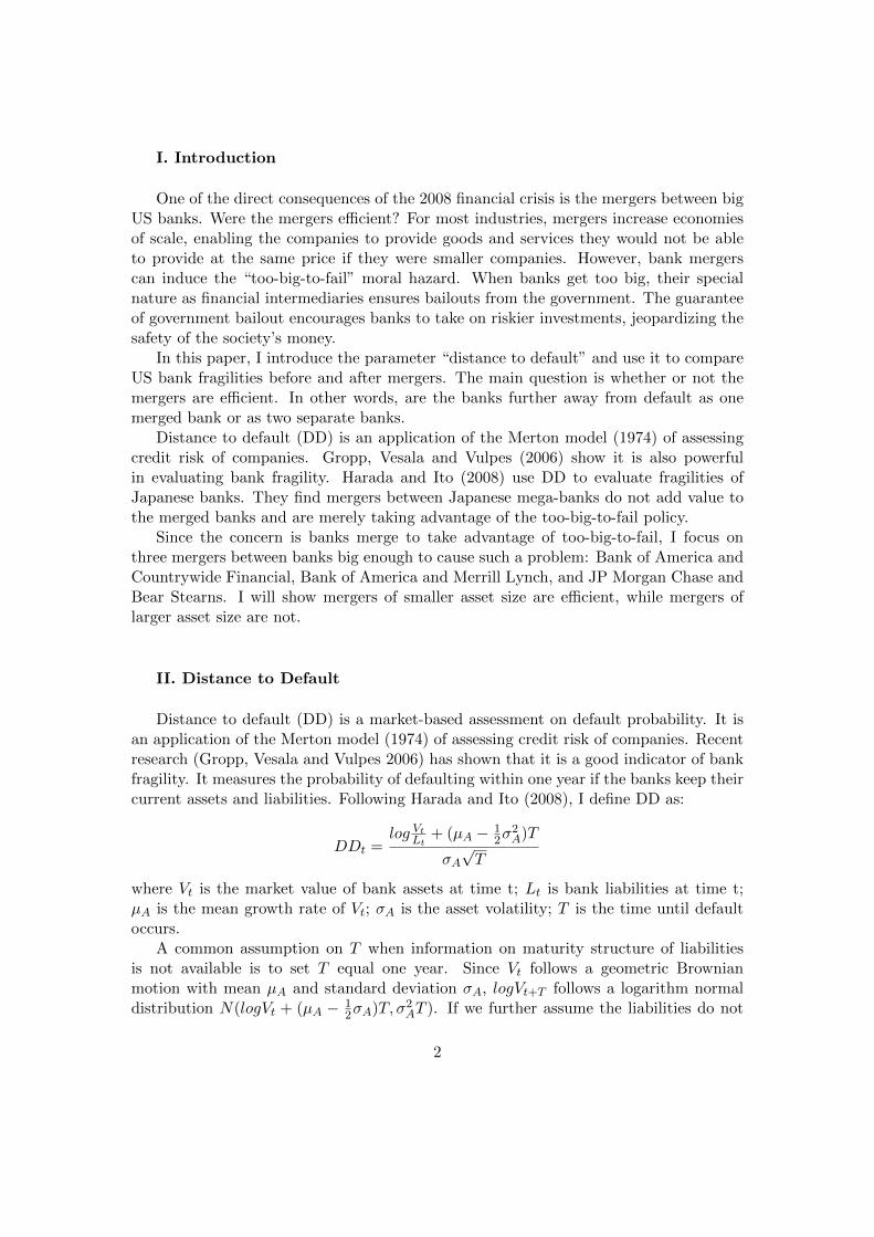
I. Introduction

One of the direct consequences of the 2008 financial crisis is the mergers between bigUS banks. Were the mergers efficient? For most industries, mergers increase economiesof scale, enabling the companies to provide goods and services they would not be ableto provide at the same price if they were smaller companies. However, bank mergerscan induce the “too-big-to-fail” moral hazard. When banks get too big, their specialnature as financial intermediaries ensures bailouts from the government. The guaranteeof government bailout encourages banks to take on riskier investments, jeopardizing thesafety of the society’s money.

In this paper, I introduce the parameter “distance to default” and use it to compareUS bank fragilities before and after mergers. The main question is whether or not themergers are efficient. In other words, are the banks further away from default as onemerged bank or as two separate banks.

Distance to default (DD) is an application of the Merton model (1974) of assessingcredit risk of companies. Gropp, Vesala and Vulpes (2006) show it is also powerfulin evaluating bank fragility. Harada and Ito (2008) use DD to evaluate fragilities ofJapanese banks. They find mergers between Japanese mega-banks do not add value tothe merged banks and are merely taking advantage of the too-big-to-fail policy.

Since the concern is banks merge to take advantage of too-big-to-fail, I focus onthree mergers between banks big enough to cause such a problem: Bank of America andCountrywide Financial, Bank of America and Merrill Lynch, and JP Morgan Chase andBear Stearns. I will show mergers of smaller asset size are efficient, while mergers oflarger asset size are not.

II. Distance to Default

Distance to default (DD) is a market-based assessment on default probability. It isan application of the Merton model (1974) of assessing credit risk of companies. Recentresearch (Gropp, Vesala and Vulpes 2006) has shown that it is a good indicator of bankfragility. It measures the probability of defaulting within one year if the banks keep theircurrent assets and liabilities. Following Harada and Ito (2008), I define DD as:

DDt =log Vt

Lt+ (µA − 1

2σ2A)T

σA√T

where Vt is the market value of bank assets at time t; Lt is bank liabilities at time t;µA is the mean growth rate of Vt; σA is the asset volatility; T is the time until defaultoccurs.

A common assumption on T when information on maturity structure of liabilitiesis not available is to set T equal one year. Since Vt follows a geometric Brownianmotion with mean µA and standard deviation σA, logVt+T follows a logarithm normaldistribution N(logVt + (µA − 1

2σA)T, σ2AT ). If we further assume the liabilities do not

2

change within a short period of time, that is Lt = Lt+T , we can rewrite DD as:

DDt =Et(logVt+T )− logLt+T

std(logVt+T )

where std(·) denotes the standard deviation. From the rewritten DD expression, theinterpretation of DD is clear. When the expected value of assets in one year equals theliabilities in one year (Et(logVt+T ) = logLt+T ), the bank reaches its default point. DDmeasures the bank’s distance to default point in terms of standard deviation of assetsvalues. A bank with DD equal to one, for example, will be one standard deviation awayfrom the default point in one year if it keeps its current assets and liabilities. A DDvalue of zero means if the bank does not change any of its financial standing then it isexpected to default in one year.

To calculate DD, I use market capitalization (stock closing price times volumestraded) to estimate Vt, short-term liabilities (the sum of customer deposits, short-termdebts, and other short-term liabilities) from banks’ income statements to estimate Lt. Iuse three years of data prior to the event windows to estimate µA and σA, with which Iassume the growth and volatility of market asset values are constant. I obtain all datafrom the Bloomberg terminal (Bloomberg 2012.)

III. Hypothesis and Data

The question I will answer is whether mergers add economies of scale to the mergedbanks. I do not attempt to answer the financial question of whether the merger makeone bank less likely to default, since it is natural to expect the better-performing bank tobecome more likely to default after it merges with the worse-performing bank. Instead,following Harada and Ito (2008), I calculate DD of a hypothetical bank constructed bysumming the assets and liabilities from the two pre-merger banks. I compare the DD ofthe hypothetical bank with the DD of the actually merged bank. The result will showif the banks are better off as two separate banks or as a merged one.

To control for market fluctuations, I use Goldman Sachs as the control bank, sinceit has not undergone any big mergers over the event windows and is of similar size asthe banks I discuss.

The null hypothesis is that the difference between DDs of the hypothetical pre-mergerbank and the control bank is the same as the difference between DDs of the post-mergerbank and the control bank. In other words, the banks are at the same distance todefault point as two separate banks and as one merged bank. The alternative to the nullhypothesis is that either banks are closer to the default point as two separate bank (inwhich case the merger is efficient,) or banks are closer to the default point as a mergedbank (in which case the merger is not efficient.)

To test the null hypothesis, I use two-sample t-test with unequal variances. The

t-statistic is t =Xpre−Xpost√

s2pre+s2post

n

with degress of freedom(s2pre+s2post)

2(n−1)

s4pre+s4post.

3

Here Xpre is the sample mean of (DDHypothetical,t − DDcontrol,t) in the pre-mergerevent window, and Xpost is the sample mean of (DDmerged,t −DDcontrol,t) in the post-merger event window. s2pre and s2post are the sample variances.

I use two event windows: 250 days pre- and post-merger, and 500 days pre- andpost-merger. The 250-day window measures the short-term effect of merger, and the500-day window measures the long-term effect.

4

Figure 1: BAC CFC 250-day Event Window

IV. Results

1. Bank of America and Countrywide Financial

Bank of America acquired Countrywide Financial on July 1, 2008. Total asset on thebalance sheet is a commonly-used indicator of bank sizes (Peek and Rosengrenb 1998.)The total size of the merger was 2.00 trillion (in US dollars) with 1.83 trillion comingfrom Bank of America and 0.17 trillion from Countrywide. The merger is considered abad financial move for Bank of America, and its stock prices went down as much as 22%within 8 days of merger. However, as I will shortly show, the merger is economicallyefficient.

For the pre-merger period I subtract DD of Goldman Sachs, the benchmark bank,from DD of a hypothetical bank combining the balance sheets of Bank of America andCountrywide Financial. For the post-merger period, I subtract DD of the benchmarkfrom DD of the newly merged Bank of America. “DD Differences” in the graphs denotesthe two differences pre- and post-merger. As previously defined, DD measures the like-lihood of defaulting within one year given the current financial conditions. A positiveDD difference indicates the bank is performing better than the benchmark; a negativeDD difference, worse.

When compared with the benchmark bank, the merged Bank of America performssignificantly better than the hypothetical pre-merger bank. Figure 1 shows how the DDsof the hypothetical pre-merger bank and the actual post-merger bank compare to theDD of the benchmark within the 250-day event window. The horizontal axis is time,

5

Figure 2: BAC CFC 500-day Event Window

Figure 3: Return on Assets BAC CFC 500-day Event Window

6

Table 1: BAC CFC 250-day t-test

t-Test: Two-Sample Assuming Unequal Variances

Pre-merger Post-mergerMean -0.344 0.031

Variance 0.005 0.010Observations 250 250

Hypothesized Mean Difference 0df 446

t Stat -47.620P(T¡=t) one-tail 0.000

t Critical one-tail 1.648P(T¡=t) two-tail 0.000

t Critical two-tail 1.965

Table 2: BAC CFC 500-day t-test


Pre-merger Post-mergerMean -0.364 0.043



t Stat -74.760P(T¡=t) one-tail 0.000



7

with days as its unit, and the vertical axis is the DD differences. The DD differencessignificantly improve after the merger on July 1, 2008. Figure 2 shows similar results forthe 500-day event window.

The formal t-tests confirm the results. For the 250-day window, the t-statistic is-47.620, rejecting the null hypothesis that there is no difference pre- and post-merger at1% level. The average DD differences from the benchmark DD improved from a negativepre-merger -0.344 to a positive post-merger 0.031. The t-statistic for the 500-day windowis -74.76, also rejecting the null hypothesis at 1% level. The improvement of DD in thelong run is even greater, from -0.364 to 0.043.

The results show surprising discrepancy between market behavior and economic pre-diction. Investors’ worry that the merger would cause the too-big-to-fail problem mightexplain part of the drop in stock price. Also, DD measures the default risk in one year,while the market focuses more on the short-term performance of the bank. To illustratethe point, I introducet the indicator ”return on assets” (ROA.) Bloomberg(2012) defines”return on assets” as the percentage:

ROAt =Trailing12MNetIncometAverageTotalAssetst

∗ 100%

where Trailing12MNetIncomet is the net income at time t calculated by adding thenet income for the most recent four quarters, and AverageTotalAssetst is the averageof the beginning and ending total assets for the quarter corresponding to time t.

Return on assets measures how profitable a bank is relative to its total assets. Itreflects the management’s ability to make earnings using bank assets at the currentperiod. The change of the return-on-assets rate also measures the efficiency of themerger, but compared to the forward-looking distance to default, return on assets reflectsthe current financial standing of the bank. Similarly as in the construction for DD, Icombine the balance sheets of Bank of America and Countrywide Financial to constructthe return-on-assets rates for a hypothetical pre-merger bank. For the post-mergerperiod, I use the return-on-asset rates for the newly merged Bank of America. I thencompare the return-on-assets rate pre- and post-merger.

Figure 3 shows the corresponding return-on-assets rates. The rate drops to its lowestaround July 1, 2008, the date of merger. Although distance to default suggests themerger is efficient, the instant drop in the return-to-assets rate causes the market torespond otherwise and explains the discrepancy between market and prediction.

2. Bank of America and Merrill Lynch

Following the acquisition of Countrywide Financial in 2008, Bank of America ac-quired Merrill Lynch on January 2, 2009. At the time of merger, the asset size of Bankof America increased to 2.32 trillion. Together with the 0.57 trillion from Merrill Lynch,the total size of the merger is 2.89 trillion, 1.44 times bigger than the combined size ofthe Countrywide merger. Contrary to the results from the last merger, DD shows Bankof America and Merrill Lynch are better off as two separate banks than as a mergedbank.

8

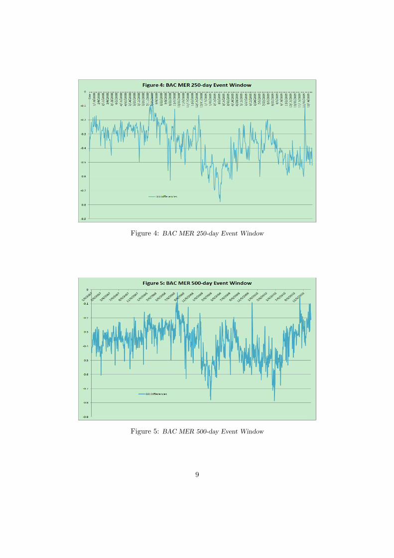
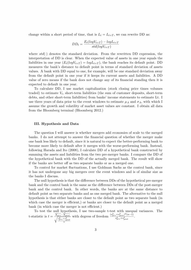
Figure 4: BAC MER 250-day Event Window

Figure 5: BAC MER 500-day Event Window

9

Table 3: BAC MER 250-day t-test


Pre-merger Post-mergerMean -0.288 -0.453



t Stat 18.994P(T¡=t) one-tail 0.000



Table 4: BAC MER 500-day t-test


Pre-merger Post-mergerMean -0.322 -0.425






10

Figure 6: JPM BSC 250-day Event Window

As before, for the pre-merger period I subtract DD of the benchmark from DD of ahypothetical bank combining the balance sheets of Bank of America and Merrill Lynch.For the post-merger period, I subtract DD of the benchmark from DD of the mergedbank. The goal is to compare the two differences.

Figure 4 shows DD differences for the 250-day event window. The DD differencesworsen after the merger on January 2, 2009, and stay worse than pre-merger for the eventwindow. This implies the merged bank performs worse than the two banks separately.The merger in fact hurts the efficiency of the two banks. The t-test (Table 3) confirmswhat we see from the graph. A t-statistic of 18.994 rejects the null hypothesis that thereis no difference in DD before and after the merger at the 1% level.

DD differences for the 500-day event window (Figure 5) show similar patterns, andt-test (Table 4) still rejects the null hypothesis at the 1% level and suggests the mergerhurts the two banks. However, the DD differences improve at the end of the eventwindow and become slightly better than the values from the pre-merger period. By theend of 2010, Bank of America has reduced its asset size from 2.89 trillion at the time ofmerger to 2.26 trillion. In the long run, the bank processes the impact through reducingits excessive size, which possibly explains the improvement of DD differences at the endof the 500-day event window.

3. JP Morgan Chase and Bear Stearns

Now I turn to JP Morgan Chase, another major player in the US banking industry.JP Morgan Chase acquired Bear Stearns on June 2, 2008. At the time of merger, its

11

Figure 7: JPM BSC 500-day Event Window

Table 5: JPM BSC 250-day t-test

Two-Sample Assuming Unequal Variances

Pre-merger Post-mergerMean 1.100 -0.054






12

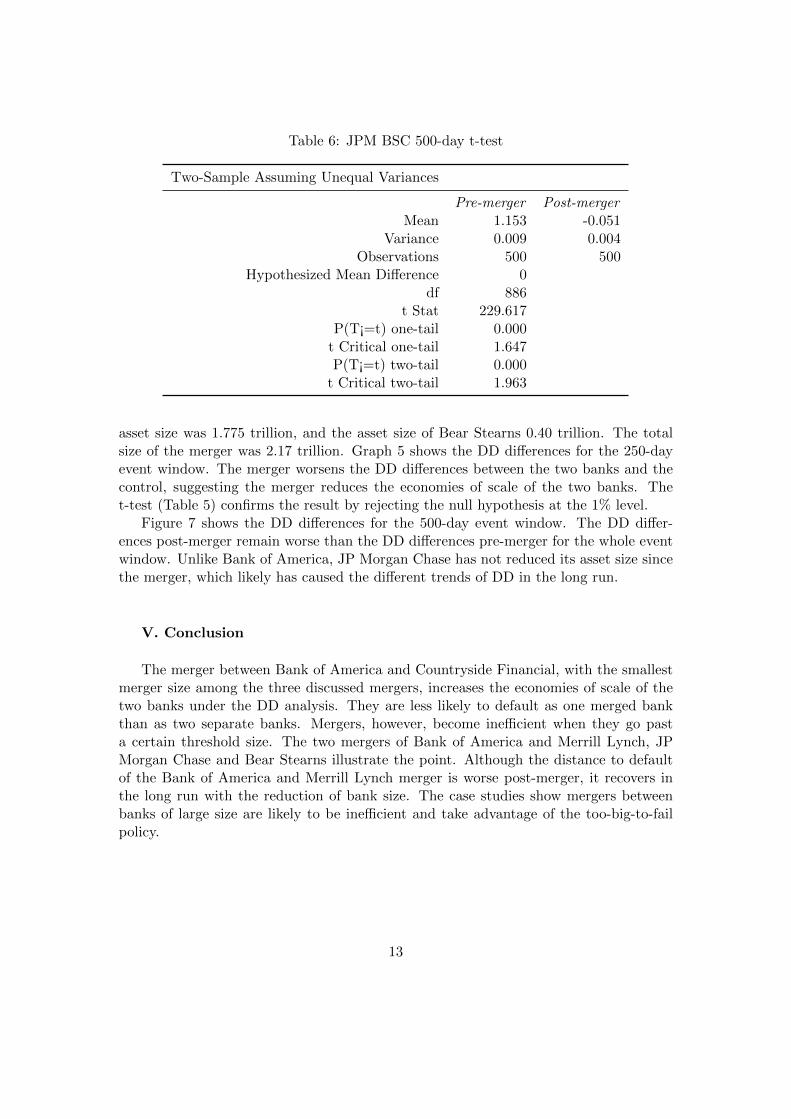
Table 6: JPM BSC 500-day t-test

Two-Sample Assuming Unequal Variances

Pre-merger Post-mergerMean 1.153 -0.051






asset size was 1.775 trillion, and the asset size of Bear Stearns 0.40 trillion. The totalsize of the merger was 2.17 trillion. Graph 5 shows the DD differences for the 250-dayevent window. The merger worsens the DD differences between the two banks and thecontrol, suggesting the merger reduces the economies of scale of the two banks. Thet-test (Table 5) confirms the result by rejecting the null hypothesis at the 1% level.

Figure 7 shows the DD differences for the 500-day event window. The DD differ-ences post-merger remain worse than the DD differences pre-merger for the whole eventwindow. Unlike Bank of America, JP Morgan Chase has not reduced its asset size sincethe merger, which likely has caused the different trends of DD in the long run.

V. Conclusion

The merger between Bank of America and Countryside Financial, with the smallestmerger size among the three discussed mergers, increases the economies of scale of thetwo banks under the DD analysis. They are less likely to default as one merged bankthan as two separate banks. Mergers, however, become inefficient when they go pasta certain threshold size. The two mergers of Bank of America and Merrill Lynch, JPMorgan Chase and Bear Stearns illustrate the point. Although the distance to defaultof the Bank of America and Merrill Lynch merger is worse post-merger, it recovers inthe long run with the reduction of bank size. The case studies show mergers betweenbanks of large size are likely to be inefficient and take advantage of the too-big-to-failpolicy.

13

References

[1] Bloomberg L.P. (2012) Retrieved March 19, 2012 from Bloomberg terminal.

[2] Gropp, Reint, Jukka Vesala, and Guiseppe Vulpes (2006): ”Equity and Bond MarketSignals as Leading Indicators of Bank Fragility.” Journal of Money, Credit & Banking38.2, 399-428.

[3] Harada, Kimie and Takatoshi Ito (2011): ”Did mergers help Japanese mega-banksavoid failure? Analysis of the distance to default of banks” Journal of the Japaneseand International Economies 25.1, 1-22.

[4] Merton, R. C. (1974): ”On the Pricing of Corporate Debt: The Risk Stucture ofInterest Rates.” Journal of Finance 29:449-70.

[5] Peek, Joe, and Eric S. Rosengren (1998): ”Bank Consolidation and Small BusinessLending: It’s Not Just Bank Size That Matters.” Journal of Banking & Finance22.6-8, 799-819.

14

were bank mergers following the 2008 financial crisis e … · were bank mergers following the 2008...

Documents