Wetland water flows and interfacial gas exchange

By

Cristina Maria Poindexter

A dissertation submitted in partial satisfaction of the

requirements for the degree of

Doctor of Philosophy

in

Engineering - Civil and Environmental Engineering

in the

Graduate Division

of the

University of California, Berkeley

Committee in charge:

Professor Evan A. Variano, Chair Professor James R. Hunt

Professor Dennis D. Baldocchi

Spring 2014

i  

Dedicated to my wonderful parents, Barbara and Bob, and also, Juliana, Diana, Jay, Tony, Hugo, Jaime, Blanche, Peggy and J.T.

ii  

Acknowledgements

I am indebted to UC Berkeley students Raymond Wong and Oliver Rickard for their invaluable assistance in the lab without which some of the research would have progressed much more slowly and inefficiently. The lab work was largely inspired by the restored wetlands on Twitchell Island. I am very appreciative of Robin Miller and Lisamarie Windham-Myers of the USGS for introducing me to the wetlands and raising important questions that guided my thinking.

Many thanks to the members of UC Berkeley biometeorology group for their very kind assistance with Twitchell Island wetland water sample collection and analysis. Special thanks to Joe Verfaillie for help troubleshooting the infrared gas analyzer and all the other components used to measure dissolved gas concentrations.

The students, post-docs and professors of the UC Berkeley environmental fluid mechanics group formed a wonderful community in which to work. I wish them all the best and hope to one day work together again. Thanks to my office mates in O’Brien Hall 202 and 205 for answering random technical question, sharing snacks, and offering encouragement through all the graduate school hurtles. Thanks to Andreas Brand and Megan Williams for instigating coffee breaks and providing thoughtful advice.

Thanks to Professors Jim Hunt and Dennis Baldocchi for their insightful suggestions for this manuscript. I referred often to their masterful course notes to better understand fundamentals of air-water gas transfer and biometeorology, respectively. Thanks to Professors Tina Chow and Mark Stacey for fluid mechanics classes that effectively tackled topics I had always wanted to understand.

Finally, utmost thanks to my research advisor, Professor Evan Variano, for his support, patience and wisdom. He generously shared his many and considerable talents for this research and manuscript and was always a pleasure to work with. He is a dedicated mentor and advocate for his students and I feel very lucky to have been one of them.

 

1

Abstract

Wetland water flows and interfacial gas exchange

by

Cristina Maria Poindexter

Doctor of Philosophy in Engineering - Civil and Environmental Engineering

University of California, Berkeley

Professor Evan A. Variano, Chair

The flow of water in wetlands may exert significant influence on wetland biogeochemistry, and particularly interfacial greenhouse gas exchange. Measuring currents in wetlands requires caution. The acoustic Doppler velocimeter (ADV) is widely used for the characterization of water flow and turbulence. However, deployment of ADVs in low-flow environments is hampered by a unique source of bias related to the ADV’s mode of operation. The extent of this bias is revealed by Particle image velocimetry (PIV) measurements of an ADV operating in quiescent fluid. Image-based flow measurement techniques like PIV may provide improved accuracy in low-flow environments like wetlands. Such techniques were applied to observe wind-driven flows in a wetland with emergent vegetation and investigate the effects of the wind shear on gas transfer across the air-water interface. Wind speed is the parameter most often used to model interfacial gas exchange in other aquatic environments. In wetlands with emergent vegetation, the emergent vegetation will attenuate wind speed above the water surface, modify fluid shear at the water surface, and influence stirring beneath the water surface. Direct measurements of gas transfer in a model wetland in the laboratory indicated that unless wind speeds are extreme, interfacial gas transfer in wetlands is typically dominated by another physical force: surface cooling-induced thermal convection. In an application of these lab results, gas transfer across the air-water interface driven by wind and thermal convection is shown to account for a sizable portion of total methane fluxes from a restored marsh in California’s Sacramento-San Joaquin Delta.

1

Chapter 1 Introduction Wetlands are defined by the presence of ponded water or saturated soils and biological signs of such conditions (e.g. hydrophitic vegetation) (National Research Council, 1995). The term wetland encompasses a range of environments from tundra to marshes to mangroves. Wetland type is set by climate as well as water chemistry. Salt marshes are superseded by mangroves in the tropics. Ombrotrophic bogs derive most of their water from precipitation while mineratrophic fens receive significant groundwater inputs (Mitsch and Gosselink, 2007). Wetlands constitute a sizeable carbon storage pool (as peat), a potentially significant annual carbon sink, and the largest single source of methane to the atmosphere (Mitsch et al., 2013; Denman et al., 2007; Gorham, 1991). What happens to extant wetlands (whether they are conserved or destroyed) and historical wetlands (whether they are restored or not) thus has important implications for climate change. For example, drainage of peat swamp forest in Indonesia led to massive peat and forest fires there in 1997. The carbon released from the peat swamps forest in 1997 represented 13-40% of mean annual global carbon emissions due to fossil fuels (Page al., 2002). Also, the drainage of marshes in the Sacramento-San Joaquin Delta has led to the oxidation of approximately 2 billion cubic meters of peat soil and counting (Mount and Twiss, 2005). Re-flooding has been shown to reverse this carbon dioxide flux, while increasing methane emissions (Hatala et al., 2012). Models for wetland carbon and methane fluxes now and into the future allow the effects of wetlands on the climate to be assessed. Ecosystem respiration of carbon dioxide is typically modeled as a function of temperature (Davidson et al., 2006) and primary production is thought to be a master variable controlling wetland methane emissions (Whiting and Chanton, 1993). Fluxes of these gases and others from wetlands may also be sensitive to the mechanism of physical transport through the water column. Gas transport in wetland water columns is unlikely to be limited to the slow pace of molecular diffusion in most cases. Instead, transport is likely driven by forces such as winds or tides. Different forces result in complex flow patterns that set transport rates via stochastic motion (i.e. turbulence) and coherent structures. For sparingly soluble gases, transport across the air water interface occurs exceedingly slowly on the water side relative to the air side. This disparity in transport rates means gas transfer models can neglect air side processes without loss of accuracy in open water (Liss and Slater, 1974). Attenuation of mean wind speed within plant canopies could inhibit transport across the boundary layer above the air-water interface. Still, observations of high turbulent kinetic energy near the base of plant canopies (e.g. Brunet et al., 1994) suggest that near surface stirring in the water remains the limiting step. Near-surface water flows are thus expected have a dominant effect on the wetland gas budget. Accordingly this research focuses on characterizing the flow in vegetated water columns and its impact on gas transport. Flow in wetlands varies to some extent with wetland type. Along channels in tidal marshes, currents on the order of 0.1 m s-1 are frequently observed (e.g. Leonard and Luther, 1995). In the low gradient Everglades, seasonally averaged (and generally unidirectional) current speeds have

2

been measured to be as low as 0.00025 m s-1 (He et al., 2010). Even where tidal or floodplain gradients are small or non-existent, other forces may lead to significant flow. Nighttime cooling of the wetland surface has been observed to cause convective currents that flush the water column in a wetland in a matter of hours (Oldham and Sturham, 2001). Wind has the potential to produce currents in wetland waters as well. Suspended sediment concentrations in the patterned ridge and slough marshes of the Everglades were found to be influenced by winds blowing along the longitudinal axis of sloughs (Noe et al., 2008). The slow flows common in wetlands present a particular challenge for measurement. Propeller-type velocimeters do not function below minimum velocity thresholds; acoustic flow measurement devices may not be as non-intrusive as previously thought. The ADV (acoustic Doppler Velocimeter), widely used since being developed in the early 1990s, generates secondary flows that may affect the accuracy of measurements in such low flows. Yet flow measurements will be important to improved understanding of the role hydrodynamic gas transport plays in wetland carbon dioxide and methane fluxes. Consequently, this thesis first addresses the question: What is the potential for a popular acoustic flow measurement device to produce biased data, particularly in slow flows like those in wetlands? Second, this thesis explores how wind and thermal convection influence air-water gas exchange in wetlands with emergent vegetation. Last, to assess the significance of interfacial gas fluxes in wetlands to total emissions of a greenhouse gas, this thesis quantifies the contribution of hydrodynamically driven air-water gas exchange to net fluxes of methane in a restored freshwater marsh. These issues are addressed in Chapter 3, 4 and 5, respectively, following an overview of air-water gas flux measurement and modeling in Chapter 2. Chapter 3 assesses the impact of acoustic streaming on flow measurement using particle image velocimetry. The probes of two different ADVs are successively mounted in a tank of quiescent water and the probes’ ultrasound emitters aligned with a laser light sheet. Observed flow is primarily in the axial direction, accelerating from the ultrasound emitter and peaking within centimeters of the velocimeter sampling volume before dropping off. The dependence of acoustic streaming velocity on ADV configuration is assessed, and it appears that different settings induce streaming ranging from negligible to more than 0.02 m s-1. From these results cases where acoustic streaming affects velocity measurements, and cases where ADVs accurately measure their own acoustic streaming are described. Chapter 4 describes experiments conducted in a model wetland in the laboratory to investigate the mechanisms and magnitude of hydrodynamic transport. Gas transfer velocities are measured while varying two drivers of gas exchange important in other aquatic environments: wind and thermal convection. To isolate the effects of thermal convection, a semi-empirical model for the gas transfer velocity as a function of surface heat loss is identified. The results indicate that thermal convection will be a dominant mechanism of air-water gas exchange in marshes with emergent vegetation. Thermal convection yields peak gas transfer velocities of 1 cm hr-1. Because of the sheltering of the water surface by emergent vegetation, gas transfer velocities for wind-driven stirring alone are likely to exceed this value only in extreme cases. Chapter 5 applies the model for the gas transfer velocity derived in Chapter 4 to investigate air-water fluxes of methane at an enclosed wetland on Twitchell Island in California’s Sacramento-

3

San Joaquin Delta. A nearly year-long water sampling campaign provides data on the dissolved methane concentrations in the marsh water column. Eddy covariance data collected by Dennis Baldocchi and his research group at UC Berkeley allow for comparison of estimated flow-driven fluxes with observed net fluxes, which also include ebullition and plant-mediated fluxes. This comparison suggests that hydrodynamic transport of dissolved gas across the air-water interface accounts for approximately 30% of net fluxes overall, and more than 50% of net fluxes at night. The improved characterization of water flow velocities and wetland gas fluxes that can be derived from this research will be useful in advancing understanding of wetland biogeochemistry, particularly as it pertains to greenhouse gas fluxes. Improved understanding is needed to inform designs of wetland restoration projects for reversing subsidence or sequestering carbon. References Bridgham, S. D., Cadillo‐Quiroz, H., Keller, J. K. & Zhuang, Q. Methane emissions from wetlands: biogeochemical, microbial, and modeling perspectives from local to global scales. Glob. Change Biol. 19, 1325-1346 (2013). Brunet, Y., Finnigan, J. J., & Raupach, M. R. A wind tunnel study of air flow in waving wheat: single-point velocity statistics. Boundary-Layer Meteorology 70, 95-132 (1994). Davidson, E. A., Janssens, I. A., & Luo, Y. On the variability of respiration in terrestrial ecosystems: moving beyond Q10. Global Change Biology 12, 154-164 (2006). Denman, K. L. et al. in Climate Change 2007: The Physical Science Basis. Contribution of Working Group I to the Fourth Assessment Report of the Intergovernmental Panel on Climate Change (eds by Solomon, S. et al.) 541-584 (Cambridge Univ. Press, 2007). Gorham, E. Northern peatlands: Role in the carbon cycle and probable responses to climate warming. Ecological Applications 1, 182-195 (1991). Hatala, J. A. et al. Greenhouse gas fluxes from drained and flooded agricultural peatlands in the Sacramento-San Joaquin Delta. Agriculture, Ecosystems and Environment 150, 1-18 (2012). He, G. et al. Factors controlling surface water flow in a low-gradient subtropical wetlands. Wetlands 30, 275-286, DOI 10.1007/s13157-010-0022-1 (2010). Liss, P. S., & Slater, P. G. Flux of gases across the air-sea interface. Nature 247, 181-184 (1974). Leonard, L. A., & Luther, M. E. Flow hydrodynamics in tidal marsh canopies. Limnology and Oceanography 40, 1474-1484 (1995). Mitsch, W. J. et al. Wetlands, carbon, and climate change, Landscape Ecol. 28, 583-597 (2012). Mitsch, W. J., & Gosselink, J. G. Wetlands (Wiley & Sons, 2007).

4

Mount, J., & Twiss, R. Subsidence, sea level rise, and seismicity in the Sacramento-San Joaquin Delta. San Francisco Estuary and Watershed Science 3, 1-18 (2005). National Research Council (U.S.) Committee on Characterization of Wetlands. Wetlands: Characteristics and Boundaries (National Academy Press, 1995). Noe, G., Harvey, J. W., Schaffranek, R. W. & Larson, L. G. Controls on suspended sediment concentration, nutrient content, and transport in a subtropical wetlands, Wetlands 30, 39-54, DOI 10.1007/s13157-009-0002-5 (2010). Oldham, C., & Sturman, J. The effect of emergent vegetation on convective flushing in shallow wetlands: Scaling and experiments, Limnol. Oceanogr. 46, 1486-1493 (2001). Page, S. E. et al. The amount of carbon released from peat and forest fires in Indonesia during 1997. Nature 420, 61-65 (2002). Whiting, G. J. & Chanton, J. P. Primary production control of methane emission from wetlands, Nature 364, 794-795 (1993).

5

Chapter 2 Background and Review of Literature 1. Introduction Many important reactions in wetlands, including aerobic respiration to methanogensis, involve the consumption and/or production of gases like oxygen, methane and carbon dioxide (Reddy and DeLaune, 2008). Quantifying fluxes of methane and carbon dioxide in wetlands is important to evaluating the impact of wetlands on the climate. Despite the importance of wetland gas fluxes, the role of wetland hydrodynamics in governing wetland air-water gas transfer has received little previous research attention. This chapter identifies major approaches to measuring and modeling gas transfer in any aquatic environment, and examines the challenges of applying these approaches and models to wetlands. 2. General concepts of air-water gas exchange In completely quiescent water column where the dissolved gas concentration C differs from the value in equilibrium with the air above, molecular diffusion results in gas transport through the bulk of the water column and across the air-water interface.

dz

dCDzJ m)( (Equation 1)

However, the molecular diffusivity of gases in water (Dm) in water is very small, on the order of 1x10-9 m2 s-1 (Hayes, 2013). In the environment, for water columns of any appreciable depth, larger scale motions of the water enhance gas transport beyond that due to molecular diffusion alone. For fully turbulent flow without local sources and sinks, the enhanced transport in the bulk of the water column can be represented as Fickian diffusion as in Equation 1, where the flux is proportional to the gradient and in the direction opposing the gradient. The turbulent diffusivity K replaces the molecular diffusivity Dm but rather than being constant, K decreases as the water surface is approached (Fisher et al., 1979). A number of simple conceptual models are used to describe the interplay of turbulent and diffusive transport near the surface and quantify the air-water gas flux as a function of the hydrodynamics. One such conceptual model for gas transfer across the air-water interface is the thin film model (Liss and Slater, 1974). The thin film model assumes that turbulent transport ceases entirely a short distance below the air-water interface at z = -. This point marks the boundary of a thin film in which transport occurs by molecular diffusion alone. For a constant flux J, solving Equation 1 for the concentration C produces a linear profile across the liquid film. The slope of the profile is equal to the concentration difference across the thin film (the gas concentration in the bulk of the water Cw minus the concentration at the interface Ca) divided by the film width .

awawmaw

mm CαCkCαCλ

D

λ

CαCD

dz

dCDzJ

0

)0( Equation 2

is the Ostwald solubility and is used to convert the concentration of the gas in the air Ca to its equilibrium concentration in the water. The Ostwald solubility is equivalent to the product of the temperature T and the universal gas constant R divided by the Henry’s constant KH (RT/KH).

6

Equation 2 shows how this simple conceptual model leads to a definition for k, the gas transfer velocity as Dm/ (Table 1). The thin film width varies spatially and temporally and thus this definition has limited practical use for the calculation air water gas transfer (Liss and Slater, 1974). However, the depth of the stagnant film can be assumed to equal the Batchelor scale ηScδB

2/1 , where is the Kolmogorov length scale and Sc is the Schmidt number (Batchelor, 1959). The Kolmogorov

scale, which marks the smallest length scale of turbulence, scales as 4/13 ενη where is the

dissipation rate of the turbulent kinetic energy and is the kinematic viscosity. Substituting the Batchelor scale for the thin film width in Equation 2 yields a relationship between k and the dissipation rate (Zappa et al., 2007) (Table 1). An alternate conceptual model for gas transfer, the surface renewal model (Higbie, 1935) relies on a different hydrodynamic variable, the time between surface renewal events. In the surface renewal model, parcels of water of concentration equal to the bulk water concentration are in contact with the air-water interface for a constant period of time equal to time between turbulent surface renewal events . Over this timescale molecular diffusion acts to equilibrate the parcel of water with the atmosphere above the water surface, yielding a Gaussian concentration profile in z across the parcel. Applying Equation 1 to this profile provides another relationship between the flux and the concentration difference and another expression for k (Table 1). A modification to the classic surface renewal model is the use of variable surface residence time . This approach requires making certain assumptions about the distribution of this time scale, for example that it has an exponential distribution (Danckwerts, 1951) or a log-normal distribution (Jahne et al., 1989). A more direct approach yields τ from the inverse of the surface divergence . Surface divergence can be related to the turbulent motions near the surface involved in transfer. From mass conservation at the surface (z=0):

γz

w

y

v

x

u

zz

00

Equation 3

Here u and v are horizontal velocities in the water while w is the vertical velocity. Substituting the surface divergence for the inverse of the surface residence time in the surface renewal model yields an expression for the gas transfer coefficient, k, where the greater the divergence at the surface, the greater is the gas flux (McKenna and McGillis, 2004; Turney et al., 2005).

7

Model for k Name Variable Source

Scνλ 1 Thin film model , the thin film width

Liss and Slater (1974)

2/14/1 Scεν Surface dissipation model , the turbulent kinetic energy dissipation rate

Lamont and Scott (1970); Kitaigorodskii, (1984)

2/1/ Scτν Surface renewal model , the surface renewal timescale

Higbie (1935)

2/1Scγν Surface divergence model , the surface divergence

McCready (1986)

Note that the thin model has been rearranged from its original form in equation 1

λ

Dk m to express k as a function of the Schmidt number.

Table 1. Conceptual models for the gas transfer velocity k Advances in measurement techniques and computational power are providing a fuller picture of the hydrodynamics of air-water gas transfer. In some respects, studies making use of these advances have found that air-water gas transfer conforms to underpinning assumptions of the conceptual models for k in Table 1. Particle image velocimetry combined with laser induced fluorescence (PIV-LIF) has been used to show how near the surface hydrodynamics are sensitive to the driver of the flow, whether it be thermal convection or shear at the bottom boundary (as in open-channel flow) (Jirka et al., 2010). This technique has also shown that for turbulence produced at the bottom boundary and transported to the near surface, coherent structures that transport water from the bulk to the surface dominate the gas flux (Variano and Cowan, 2013), a finding that validates the emphasis on surface renewal time scale by the surface renewal model. Furthermore, detailed measurements using particle image velocimetry of surface divergence (Turney et al., 2005; McKenna and McGillis, 2004) along with air-water gas flux indicate that this model accurately predicts flux for a range of flow types. While the relationship between hydrodynamic variables and gas transfer remains an area of active research, the gas transfer velocity k can still be defined most generally as flux across the air-water interface J(z=0) divided by the dissolved gas concentration difference across the air-water interface (after accounting for solubility effects).

aw CαC

zJk

)0(

(Equation 4)

By this definition k encompasses all the near surface hydrodynamics responsible for gas transfer. The sensitivity of the gas transfer velocity to the molecular diffusivity or the Schmidt number of the gas in question (as shown in Table 1) means that k must be adjusted when measured or modeled for one gas but applied to another. Schmidt number (Sc) scaling (Equation 5) is used to scale gas transfer velocities. By convention gas transfer velocities reported in the literature are

8

typically scaled to indicate the equivalent gas transfer velocity for carbon dioxide gas at 20 C, which has a Schmidt number of 600.

n

Sckk

600600 (Equation 5)

The Schmidt numbers for several gases of ecological importance and other gases often used as tracers (for gas transfer velocity measurement) are shown in Table 2 (Hayes, 2013; King and Saltzman, 1995).

Gas Sc CH4 620 CO2 600 He 150

N2O 470 O2 500 Rn 890 SF6 950

Table 2. Schmidt numbers at 20 C

While the hydrodynamics controlling air-water gas transfer as measured in the lab can help explain the mechanisms of air-water gas transfer under controlled conditions, measurements of air-water gas fluxes in the environment are needed to understand how flow and other factors interact to generate fluxes. 3. Methods to measure air-water gas exchange Floating or static chambers are perhaps the simplest and cheapest method to measure air-water gas exchange and thus, not surprisingly, they have been very widely used in wetlands (e.g. Miller, 2011), lakes (Guerin et al., 2007), estuaries (e.g. Borges et al., 2004) and the ocean (e.g. Frankignoulle, 1988). After the chamber is placed over the water surface, the rate of change in headspace gas concentrations with time is used to determine the flux. Gas concentrations are measured with a gas chromatograph or infrared gas analyzer. Where ebullition occurs in addition to dissolved gas exchange across the air-water interface, substantial instantaneous increases in the headspace concentration must be disregarded in the calculation of the rate of change in the headspace concentration (e.g. Matthews et al., 2003). While some data suggest that chambers provide accurate results at low wind speeds (Kremer et al., 2003), other data indicate that the turbulence created by the bobbing of a floating chamber has the potential to bias gas transfer measurements for low wind speeds in particular (Vauchon et al., 2010). Phytochambers, chambers that are placed over plants to measure fluxes both across the air-water interface and through the plant stomata, have been used frequently in wetlands with emergent vegetation (e.g. Miller, 2011; Chanton et al., 1993). An assessment of this method suggests that the chambers themselves can quickly alter concentration, temperature and humidity gradients, thus requiring very short measurement periods (Knapp and Yavitt, 1992). While there is debate

9

about whether chamber based methods are intrusive, there is agreement that chambers have the limitation of low temporal resolution, a disadvantage that can be particularly problematic for the understanding of mechanisms of gas transfer and its variability. The eddy covariance technique offers many advantages for measuring fluxes. Eddy covariance data is quasi-continuous, spans long time-periods and is spatially-integrated and non-intrusive. Disadvantages include under-sampling at night when winds tend to be light or intermittent (Baldocchi, 2003), the high cost of the equipment and its long-term maintenance and the difficulty of measuring small areas (because of changing footprints). There are numerous examples of studies where eddy covariance has been used to measure CO2 and methane fluxes from wetlands including Lafleur et al. (2005), Bonneville et al. (2008), Hatala et al., (2012) and Godwin et al. (2013). Eddy covariance can provide air-water gas flux data sets of unparalleled length and temporal resolution. In wetlands with emergent vegetation, the net flux measured via eddy covariance includes not only air-water gas transfer of CO2 and CH4 but also plant mediated fluxes (and may also include ebullitive fluxes for CH4). In this situation, measuring net fluxes in a simulated wetland in the laboratory with artificial vegetation (as is described in Chapter 4) allows for the isolation of the air-water gas flux. In addition measuring air-water gas fluxes in laboratory flumes can improve understanding of physical gas exchange mechanisms because it allows for greater control of ambient conditions. Laboratory flux measurements also permit detailed measurements of the water flow and dissolved gas concentration field with techniques that are not viable outside the laboratory, like particle image velocimetry combined with laser induced fluorescence (Variano and Cowan, 2013). A key disadvantage of laboratory air-water gas flux measurement is that it can be difficult to recreate in the laboratory some natural phenomenon like oceanic scale wave (Jahne et al., 1987) or the coherent structures occurring within a plant canopy beneath a stable or unstable atmosphere (Dupont and Patton, 2012). Quantifying gas transfer using the gas transfer velocity is another way to isolate air-water gas fluxes from other fluxes measured by the eddy covariance technique and this is the approach taken in Chapter 5. This approach requires accurate values for the gas transfer velocity. 4. Gas transfer velocity measurement A number of techniques have been used to measure the gas transfer velocity, from the intentional release of tracers in the environment to measurements of turbulent kinetic energy dissipation and application of the surface dissipation model. Furthermore, any method used to measure air-water gas flux can be combined with dissolved gas measurements to estimate k according the definition in Equation 4. Each method has its advantages and disadvantages. One downside of using tracer releases to measure the gas transfer velocity is that this method produces gas transfer velocity data of low temporal resolution (on the order of days) (Wanninkhof et al., 2004) while environmental conditions like wind speed vary over much shorter time scales. Nonetheless, for wetlands, where the multiple flux pathways make measurement of k with eddy covariance data difficult, tracer release may be the most straightforward, non-intrusive method for obtaining a gas transfer velocity and in turn the air-water gas flux.

10

Method Equation used to determine k Example Definitions Tracer release (well mixed conditions)

af

aiSF SFαSF

SFαSF

t

hk

66

66lnΔ6

Harrison et al., 2012

[SF6]i ,[SF6]f = initial, final tracer concentration in the water. [SF6]a = tracer concentration in the air.

Tracer release (non-well mixed conditions)

h

tk

tK

y

tK

Utx

KKπ

M

tyxSF

SF

yxyx

6

44

)(exp

4

),,(

20

6

Variano et al., 2009

M0 = initial mass of tracer released, Kx and Ky = dispersion coefficients in the x and y directions, U is the mean velocity in the x direction.

Dual tracer release

nSFHe

f

i

He ScSc

SFHe

SFHe

t

h

k

6

3

3

1

lnΔ 6

36

3

Wanninkhof et al., 2004

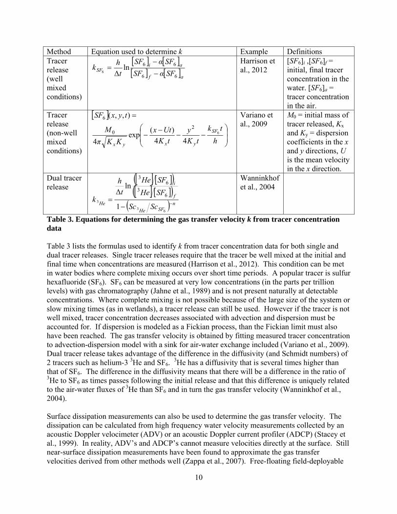
Table 3. Equations for determining the gas transfer velocity k from tracer concentration data Table 3 lists the formulas used to identify k from tracer concentration data for both single and dual tracer releases. Single tracer releases require that the tracer be well mixed at the initial and final time when concentrations are measured (Harrison et al., 2012). This condition can be met in water bodies where complete mixing occurs over short time periods. A popular tracer is sulfur hexafluoride (SF6). SF6 can be measured at very low concentrations (in the parts per trillion levels) with gas chromatography (Jahne et al., 1989) and is not present naturally at detectable concentrations. Where complete mixing is not possible because of the large size of the system or slow mixing times (as in wetlands), a tracer release can still be used. However if the tracer is not well mixed, tracer concentration decreases associated with advection and dispersion must be accounted for. If dispersion is modeled as a Fickian process, than the Fickian limit must also have been reached. The gas transfer velocity is obtained by fitting measured tracer concentration to advection-dispersion model with a sink for air-water exchange included (Variano et al., 2009). Dual tracer release takes advantage of the difference in the diffusivity (and Schmidt numbers) of 2 tracers such as helium-3 3He and SF6.

3He has a diffusivity that is several times higher than that of SF6. The difference in the diffusivity means that there will be a difference in the ratio of 3He to SF6 as times passes following the initial release and that this difference is uniquely related to the air-water fluxes of 3He than SF6 and in turn the gas transfer velocity (Wanninkhof et al., 2004). Surface dissipation measurements can also be used to determine the gas transfer velocity. The dissipation can be calculated from high frequency water velocity measurements collected by an acoustic Doppler velocimeter (ADV) or an acoustic Doppler current profiler (ADCP) (Stacey et al., 1999). In reality, ADV’s and ADCP’s cannot measure velocities directly at the surface. Still near-surface dissipation measurements have been found to approximate the gas transfer velocities derived from other methods well (Zappa et al., 2007). Free-floating field-deployable

11

particle image velocimetry (PIV) has also been used to characterize profiles of dissipation with depth at the surface and very short distances from the surface (Wang et al., 2013). The use of this technique eliminates the need to use dissipation rates measured below the surface to represent surface dissipation. The spatially resolved velocity data produced by particle image velocimetry can also be used to measure the surface divergence if images are taken parallel to the water surface and reflections from the surface are minimized. Obtaining dissipation and surface divergence data and conducting tracer releases and sampling can require considerable time and expense. Scaling relationships for the dissipation can be used to predict gas transfer velocity from dissipation without conducting any measurements. When

wind stress dominates the production of turbulence, the dissipation in the ocean scales with zκ

u3*

where z is the distance from the surface, is the von Karman constant and u* is the shear velocity at the surface on the water side. On the other hand, when buoyancy controls turbulence production, the dissipation scales with the buoyancy production, which is constant with depth

(Lombardo and Gregg, 1989). The buoyancy production is calculated asρc

βqgB

p

where q is the

surface heat loss, g the acceleration due to gravity, the expansivity of water, cp the isobaric heat capacity and the density. Complicating this approach to quantifying surface dissipation is the effect of waves on surface dissipation. Beneath the water surface in lakes, if the wave field is not fully developed, there is shallow region where the dissipation profile is nearly constant and does not follow the shear production scaling (Wüest and Lorke, 2003). Non-fully developed wave fields are the norm in all but the largest lakes and, of course, the ocean (Wüest and Lorke, 2003). Applying scaling relationships where there is no one dominant source of turbulent kinetic energy dissipation is possible but such scalings can be very unwieldy (e.g. Soloviev et al., 2007). In wetlands with emergent vegetation, wake production rather than shear production drives turbulent kinetic energy production throughout most of the water column. In tidal wetlands, dissipation has been observed to scale with aCU D

3 where U is the mean velocity, CD the drag

coefficient (1) and a the frontal area of vegetation per unit volume (Nepf, 2012). Deviations from this scaling have been observed near the water surface due to wind (Lightbody and Nepf, 2006). Empirical models for the gas transfer velocity predict k from easily measured parameters such as the wind speed. These models can be used to quantify air-water water gas fluxes where direct measurement of air-water gas flux, direct measurement of the gas transfer velocity or scaling of the dissipation is not feasible.

12

5. Empirical models for the gas transfer velocity

Model Environment Method Reference CitedWind

k660 = 0.31(U10)2 Ocean Tracers Wanninkhof,

1992 1679

k660 = 0.0283(U10)3 Ocean Eddy

covariance Wanninkhof & McGillis, 1999

340

k600 = 2.07+0.215(U10)1.7 Lake Tracers Cole and

Caraco, 1998

447

Thermal convection

k500 = 6.293 x 10-7q2+1.036 x 10-6q Lake Lab Schladow et al., 2002

16

Rain k600 = 2.48+65.46KEF-21.81KEF2 Ocean Lab Ho et al.,

1997 46

Wind and current k500 = 1.792(u*b

3/h)0.336+0.0375u*a (u*a<0.20 m s-1) k500 = 1.792(u*b

3/h)0.336+0.00183u*a2

(u*a>0.20 m s-1)

River Lab Chu and Jirka, 2003

16

Wind and thermal convection k600 = 2.0+2.04U10 (q<0) k600 = -0.15+1.74U10 (q>0)

Lake Eddy covariance

MacIntyre et al., 2010

14

Wind and rain k600 = 0.1414(U10)

2+ (1-exp(0.3677*(KEF/au*a

3))*63.02(KEF)0.6242

Ocean Lab Harrison et al., 2012

1

k, gas transfer velocity in cm hr-1 (except for Schladow (2002) which is in m d-1); 600, Schmidt number for CO2 at 20 C in fresh water; 660, Schmidt number for CO2 at 20 C in sea water; 500, Schmidt number for O2 at 20 C in freshwater; U10, wind at 10 m height in m s-1; q, heat flux in W m-2; KEF, kinetic energy flux of rain in J m-2 s-1 ; h, depth; u*b , shear velocity at bottom boundary; u*a, shear velocity in air Table 4. Empirical models for gas transfer velocity: a sampler of the leading models for k as a function of wind speed and a few available models for other environmental drivers of gas transfer. Table 4 shows a number of different empirical relationships for the gas transfer velocity. For each relationship listed, the second column shows the aquatic environment in which the relationship is meant to be applied and the third column shows the method used to obtain the relationship. The last column shows the number of times the model has been cited in Web of Science. This list of gas transfer velocity relationships is not comprehensive, particularly in regards to relationships for k as a function of wind speed. The table does show three highly cited

13

relationships that remain in wide use (Wanninkhof, 1992; Wanninkhof and McGillis, 2003; Cole and Caraco, 1998). These three relationships have been cited hundreds of times, reflecting the dominance of wind as a driver of gas transfer in the ocean and larger lakes. Wind generates near surface turbulence directly from wind shear and instabilities, but also creates wind waves, which generate near-surface turbulence (Bock et al., 1999). Increased air-water gas exchange can occur when waves break, forming bubbles. A recently derived cubic function of wind speed proposed by Edson et al. (2011) for the gas transfer velocity, better fits the limited data for air-water gas transfer at high winds, for which bubble formation by breaking waves enhance gas transfer. At low wind speeds in non-fluvial aquatic systems, other drivers of gas transfer such as surface cooling and rain become important. An empirical model for the gas transfer velocity as a function of heat loss developed in the laboratory and intended for use in lakes indicates a quadratic relationship (Schladow et al., 2002). Rain may be as important as wind in rainy regions like the tropics. The effect of rain on gas transfer is parameterized by Ho et al. (1997) using the kinetic energy flux due to rain or KEF. KEF can be converted to rain rate R (in mm hr-1) using a raindrop size distribution such as that of Marshall and Palmer (1948) which produces KEF = 0.00343R1.17 or the Laws-Parsons distribution (Harrison et al., 2012) which produces the relationship KEF =0.0112R. To represent the effect of multiple driving forces of gas transfer, some have assumed that various driving process are simply additive. For example, Chu and Jirka (2003) combined an empirical relationship for the gas transfer velocity as function on shear velocity in the air with another empirical relationship for gas transfer velocity as a function of bottom boundary shear velocity. This combination model accurately predicted the gas transfer velocity in a sloping flume equipped with a wind tunnel over the range of wind and bottom boundary shear tested. The effects of different environmental forcings may not be additive in all cases however, at least within certain ranges. Harrison et al. (2012) proposed non-additive relationship between wind and rain in the ocean and three different regimes, a rain dominated regime, a wind dominated regime and a regime where both process act together. The complexity of identifying the boundaries between regimes where different driving processes dominate and the behavior of different driving forces of gas transfer of equal importance highlights the limitations of empirical models. Empirical relationships in Table 4 and others like them have been widely applied, e.g. for the prediction of patterns CO2 flux across the world’s oceans (Takahashi et al., 2002). Still there remains some uncertainty about the relationship between gas transfer and wind speed and a lot of scatter in the data. Some of this scatter can be explained by water chemistry, particularly the presence or absence of surfactants. 6. Roles of surfactants and chemistry Surfactants are often present in natural waters, for example in and around phytoplankton blooms in the ocean and in environments with high concentrations of dissolved humic substances (Frew et al., 1990). Surfactants modify the near-surface hydrodynamics in a number of different ways that all lead to reduced air-water gas transfer. The major effect of surfactants is reduction in surface tension and an increase in elasticity that prevents subsurface motions from extending to

14

the interface (Lee and Saylor, 2010). More specifically, numerical simulations indicate that that surfactant contamination leads to: (1) increased shear (u/z) just below the surface, (2) decreased root-mean-square horizontal velocities (urms and vrms) just below and at the surface and (3) increased x- and y- vorticity at the surface because of variation in surfactant concentration (Khakpour et al., 2011). Experiments in laboratory wave tanks suggest that waves are also affected. It is the smallest (less than 0.01 m) waves that are most important for gas transfer. Surfactants damp very short waves (wave numbers above 100 rad m-1) completely eliminate the shortest waves (Bock et al., 1999). While the empirical relationships for gas transfer listed in Table 4 do not adjust for the presence of surfactant, the surface divergence and surface dissipation models for the gas transfer velocity listed in Table 1 can be adjusted by using an exponent of -2/3 for the Schmidt number rather than -1/2 (Jahne et al., 1987). Chemical enhancement of CO2 air-water gas transfer occurs because of the chemical reactions that transform dissolved CO2 to bicarbonate and bicarbonate to carbonate as pH increases. Chemical enhancement of the gas transfer velocity may need to be accounted for, particularly at high pH when CO2 fluxes are of interest. Chemical enhancement may be of particular importance in low turbulence, high temperature water bodies where it may double the flux. In warm alkaline lakes, enhancement can account for nearly the entirety of the flux (Wanninkhof and Knox, 1996). It is less important in cooler systems where the gas transfer velocity is above high. Enhancement factors are applied directly to the gas transfer velocity and can be predicted theoretically from the rate constants for the reactions of the carbonate system (Hoover and Berkshire, 1969). Chemical enhancement could be important in wetlands with areas of open water were submerged and floating plants elevate the pH via intake of CO2 during photosynthesis but are less likely to be important wetlands with emergent vegetation. In the end, water chemistry and specifically the level of disequilibrium between the air and the water, is as important as the gas transfer velocity in determining air-water gas transfer. Reliable and sturdy sensors to measure dissolved concentrations continuously in the water are long established for some gases like oxygen and barely on the horizon for others like methane. Optical oxygen measurement ameliorates some of the limitations of the popular Clark electrode oxygen method for oxygen measurement. Optical measurements do not consume oxygen during measurement and thus do require mixing adjacent to the sensor to achieve accurate measurements (Ramamoorthy et al., 2003). Dissolved CO2 probes that are continuous were only recently tested in natural waters by Johnson et al. (2010) and found to provide accurate data. Continuous methane sampling is possible but requires a bulky and sensitive apparatus that includes an equilibrator (Gulzow et al., 2011). While this type of system has been used in lakes (Del Sontro et al., 2013), it has not yet been used in wetlands. 7. Complexities of measuring and modeling air-water gas transfer in wetlands with emergent vegetation

Figure 1concentrwater inhigh shewhere dathe air-windividu Figure 1 vegetatiocomplicaabove ancompared

. Schematiration (g,h) terface (z<=ar velocity)ata are avai

water interfaal subplots.

illustrates soon, particularated, relativend below the d to the clas

c of the winin and abov

=0). Differe and at nighilable. For race in tidal .

ome of the crly non-tidale to air-water

water surfacs log layer.

nd (a), curreve a wetlandent profiles ht (stable atreference, swetlands ar

complexities l wetlands. Ur gas transferce. The emeThe log laye

15

ent(b), turbud’s emergenfor the day tmosphere asample profre also show

of modelingUnderstandinr in lakes or ergent canoper is displace

ulence(c,d),nt canopy (z(neutral atm

and low shefiles of currewn. See Tab

g gas transfeng gas transoceans, by t

py physicallyed upwards b

, temperatuz>=0) and bmospheric car velocity)ent and turbble 5 for det

er in wetlandfer in wetlanthe presencey alters the wby a displac

re (e,f) and elow its air-conditions a) are shown bulence belotails on

ds with emernds is e of vegetatiowind profile ement heigh

CO2 -and

ow

rgent

on

ht d

16

(Figure 1a). For neutral atmospheric conditions, mean wind speed through the vegetation decreases exponentially at a rate that is sensitive to the flexibility and density of the vegetation (Cionco, 1972). Near the base of some vegetation canopies, a secondary wind maximum (SWM) has been observed (e.g. Baldocchi and Meyers, 1988). Within a stably stratified atmosphere, which often occurs at night, a decoupling of the flow above and below the canopy has been observed (Jacobs et al., 1994). Evidence of this decoupling is visible in the nighttime temperature profiles within and above the canopy in Figure 1e. For stable atmospheric conditions, the appropriate scale for the mean wind speed within the canopy is no longer the shear velocity but the convective velocity w* = (BH)1/3, where B is the buoyancy production and H is the canopy height (Jacobs et al., 1994). As shown in Figure 1a, the convective velocity (for a reasonable surface heat flux q=200 W m-2) is of similar to scale to the velocity predicted by the exponential decay of the mean wind speed at the top of the canopy. In sum, the unique properties of mean wind speed within vegetation canopies: (1) exponential decay of mean wind speed, (2) secondary wind maxima and (3) decoupling from the atmospheric boundary layer under stable conditions, make mean wind speeds above the water surface in a wetland with emergent vegetation very different from those likely to occur over open water. This suggests that the empirical relationships for gas transfer velocity as a function mean wind speed at 10 m shown in Table 4 are unlikely to apply to air-water gas transfer in wetlands with emergent vegetation. The rapid decay of mean wind speed through the top of the vegetation canopy leads to very high shear in this region, which in turn results in a jump in the production of turbulent kinetic energy and generation of Kelvin-Helmholtz instabilities (Raupach et al., 1996). The turbulent kinetic energy production is evident in the peak in the dissipation of turbulent kinetic energy at the canopy top in Figure 1c. Within the canopy, turbulent kinetic energy is produced in the wakes of vegetation stems. Because of the small scale of this wake produced turbulent kinetic energy, it dissipates quickly (Raupach et al., 1996). Nevertheless, turbulent kinetic energy remains high near the air-water interface due to transport from the canopy top, and frequent flow reversals occur (Brunet et al., 1994). The implications of these features of the turbulence near the air-water interface on gas transfer are not known. Heat loss from the water surface may result in mixing within the water column. Figure 1f shows temperature data at two points within the surface water at re-established wetlands on Twitchell Island (at the surface and 0.18 m below the surface) recorded in March 2006 (Miller and Fujii, 2010). While the shape of the profile of temperature with depth is not known between these two points, the data do indicate stably stratified conditions during the day, with surface water temperature exceeding the temperature at depth by more than 5 C. At night the water column temperatures are the same at the surface and at depth, raising the possibility that cooling at the water surface has resulted in thermal convection and mixing across the water column. Figure 1b shows the wind driven velocity measured using a prototype Volumetric Particle Imager (Tse and Variano, 2013) at two depths within the re-established wetlands on Twitchell Island on April 9, 2013. Wind speeds were extraordinarily high this day, yet mean horizontal water speeds are on the order of only 0.001 m s-1. These velocities are of the same order of a magnitude as the convective velocity scale in the water w* = (Bh)1/3 where B is the buoyancy production in the water and h is the surface water depth. On days when winds are light or

17

average, water flow velocities were observed to be an order of magnitude lower. While there is insufficient data deeper within the water column to determine whether a log layer exists within the surface water as it does in lakes exposed to winds (Wüest and Lorke, 2003), the data suggest a boundary layer of at least 0.05 m. We can draw this conclusion due to the nature of flow observed. The mean horizontal speed is 0.001 m s-1 but the mean velocity is an order of magnitude lower. This is because the mean horizontal velocity was characterized by frequent flow reversals. Interestingly, flow reversals are also a characteristic of the flow at the base of vegetation canopies. Scaling relationships for dissipation that have been tested in tidal wetlands with high water flow velocities (Nepf et al., 1999; Lightbody and Nepf, 2006) may not apply for the low mean currents in some non-tidal wetlands (Figure 1b). As a point of comparison, Figures 1b and 1d show profiles of water current and turbulent kinetic energy dissipation for a wetland exposed to a tidal gradient of 0.0001 m m-1. This gradient is of the same order of magnitude that has been observed in tidal salt marshes in the east and west coasts of the United States (French and Stoddart, 1992). The tidal current, observed at a salt marsh in the Plum Island Estuary, Massachusetts (Lightbody and Nepf, 2006) and scaled to a tidal gradient of 0.0001 and water depth of 0.25 m, is fairly uniform through the water column except near the bed, where there is small shear layer. The tidal current for this tidal gradient is at least an order of magnitude larger than the convective velocity scale or the measured wind-driven currents at the restored wetland on Twitchell Island. The dissipation rate calculated from the velocity and the scaling relationship tested by Nepf (1999) is shown in Figure 1d. This dissipation rate is many several orders of magnitude greater than the dissipation in a thermal convective wetland water column. No data for the dissipation profile in a wetland water column due to wind was available. A hypothetical CO2 concentration profile within the emergent canopy, shown in Figure 1g, is derived from measurements of CO2 in a soy canopy in 1974 (Baldocchi, 1992) scaled using the height of the emergent wetland plant canopy and to contemporary atmospheric CO2 levels. This profile is characterized by elevated CO2 at the base of the canopy, and lower levels near the top of the canopy due to uptake during photosynthesis. The shape of the profile, which has also been observed in forests canopies at certain times of day (Koike et al., 2001; Brooks et al., 2007), points to a potential pitfall in the modeling of wetland air-water gas transfer using the gas transfer velocity and the air-water concentration gradient. If CO2 concentrations in the air are measured above the canopy even though CO2 concentrations near the base of the vegetation canopy (and above the air-water interface) are much higher, air-water fluxes of CO2 calculated using a gas transfer velocity could be overestimates. The CO2 concentration profile in the water (Figure 1h) indicates a water column that is supersaturated with respect to the atmosphere. The water surface concentration is equal to the concentration in equilibrium with the air above while the concentration below the surface has been set equal to the average dozens of dissolved CO2 measurements made in 2012 and 2013 (and described in further detail in Chapter 5).

18

Table 5 Additional details on data and models used for plotting profiles in Figure 1 Figure 1a

Canopy height H = 3 m, displacement height = 0.6H, roughness height = 0.1H, decay constant for exponential flow through vegetation, 2 m-1 Day: Shear velocity u* = 0.45 m s-1, neutral atmosphere. Night: Shear velocity u* = 0.15 m s-1, Obukhov length scale L = 50 m, log-layer modified by Businger-Dyer relationships, convective velocity w* = (BH)1/3, where B is the buoyancy production and H is the canopy height. B = gq/(Tcp) where q = 200 W m-2, T = 20C.

Figure 1b

Convective velocity scale w* = (Bh)1/3, where B is the buoyancy production and h is the water depth. B = gq/(cp) where q = 200 W m-2 and is the expansivity of water. Tidal currents profile from observations at the Plum Island Estuary, Massachusetts (Lightbody and Nepf, 2006) and scaled using the velocity Um = [hg(dh/dx)]1/2 with dh/dx=0.0001 and h=0.25 m.

Figure 1c

Day: Dissipation of turbulent kinetic energy observed by Brunet et al. (1994) for an artificial wheat canopy in a wind tunnel and scaled to a canopy height 3 m and shear velocity 0.45 m s-1. Night: Dissipation rate within the canopy is expected to equal the buoyancy production.

Figure 1d

Tidal wetland: dissipation calculated from the scaling relationship, = U3CD/d where U is the tidal current speed from Figure 1b, CD is the drag coefficient. The plant volume density =0.02 and the stem diameter = 0.01 m.

Figure 1e

Dupont and Patton’s (2012) measured profiles of temperature as a percentage of temperature at the canopy top H within a walnut tree canopy for neutral and stable conditions. The data have been scaled to a canopy height of 3 m.

Figure 1f CO2 concentration profile within the emergent canopy derived from measurements of CO2 in a soy canopy in 1974 (Baldocchi, 1992) scaled to an emergent wetland plant canopy height of 3 m and to contemporary atmospheric CO2 levels.

Figure 1g Water surface concentration is equal to the concentration in equilibrium with contemporary atmospheric CO2 levels while the concentration below the surface has been set equal to the average of dissolved CO2 measurements made 5 cm below the water surface in 2012 and 2013 (and described in further detail in Chapter 5).

References Baldocchi, D. D., & Meyers, T. P. Turbulence structure in a deciduous forest. Boundary-Layer Meteorology 43, 345-364 (1988). Baldocchi, D. D. Assessing the eddy covariance technique for evaluating carbon dioxide exchange rates of ecosystems: past, present and future. Global Change Biology 9, 479-492 (2003). Baldocchi, D. D. A Lagrangian random-walk model for simulating water vapor, CO2 and sensible heat flux densities and scalar profiles over and within a soybean canopy. Boundary-Layer Meteorology 61, 113-144 (1992).

19

Batchelor, G. K. Small-scale variation of convected quantities like temperature in turbulent fluid. Part 1: General discussion and the case of small conductivity. J. Fluid Mech. 5, 113–133 (1959). Bock, E.J., Hara, T., Frew, N.M. & McGillis, W.R. Relationship between air sea gas transfer and short wind waves. J. Geophysical Research 104, 25–25 (1999). Bonneville, M. C., Strachan, I. B., Humphreys, E. R., & Roulet, N. T. Net ecosystem CO2exchange in a temperate cattail marsh in relation to biophysical properties. Agricultural and Forest Meteorology 148, 69-81 (2008). Borges, A. V. et al. Variability of the gas transfer velocity of CO2 in a macrotidal estuary (the Scheldt). Estuaries 27, 593-603 (2004). Brooks, J. R., Flanagan, L. B., Varney, G. T., & Ehleringer, J. R. Vertical gradients in photosynthetic gas exchange characteristics and refixation of respired CO2 within boreal forest canopies. Tree Physiology 17, 1-12 (1997). Brunet, Y., Finnigan, J. J., & Raupach, M. R. A wind tunnel study of air flow in waving wheat: single-point velocity statistics. Boundary-Layer Meteorology 70, 95-132 (1994). Chanton, J. P., Whiting, G. J., Happell, J. D., & Gerard, G. Contrasting rates and diurnal patterns of methane emission from emergent aquatic macrophytes. Aquatic Botany 46, 111-128 (1993). Chu, C. R., & Jirka, G. H. Wind and stream flow induced reaeration. Journal of Environmental Engineering 129, 1129-1136 (2003). Cole, J. J. & Caraco, N. F. Atmospheric exchange of carbon dioxide in a low-wind oligotrophic lake measured by the addition of SF6, Limnol. Oceanogr. 43, 647-656 (1998). Cionco, M. A wind-profile index for canopy flow. Boundary-Layer Meteorology 3, 255–263 (1972). Culberson, S. D., Foin, T. C., & Collins, J. N. The role of sedimentation in estuarine marsh development within the San Francisco Estuary, California, USA. Journal of Coastal Research 20, 970-979 (2004). Danckwerts, P. V. Significance of liquid film coefficients in gas absorption. Ind. Eng. Chem. 43. 1460–67 (1951). Del Sotro, T., Sollberger, S., Kling, G., Shaver, G. R. & W. Eugster. High Resolution CH4 Emissions and Dissolved CH4 Measurements Elucidate Surface Gas Exchange Processes in Toolik Lake, Arctic Alaska, Abstract B52B-02 presented at 2013 Fall Meeting, AGU, San Francisco, Calif., 9-13 Dec (2013).

20

Dupont, S., & Patton, E. G. Influence of stability and seasonal canopy changes on micrometeorology within and above an orchard canopy: The CHATS experiment. Agricultural and Forest Meteorology 157, 11-29 (2012). Fisher, H. B., List, E. J., Koh, R. C. Y., & Imberger, J. Mixing in Inland and Coastal Waters (Brooks, 1979). Frankignoulle, M. Field measurements of air-sea CO2 exchange. Limnol. Oceanogr. 33, 313–322, doi:10.4319/lo.1988.33.3.0313 (1988). French, J. R., & Stoddart, D. R. Hydrodynamics of salt marsh creek systems: Implications for marsh morphological development and material exchange. Earth surface processes and landforms 17, 235-252 (1992). Frew, N. M., Goldman, J. C., Dennet, M. R. & Johnson, A. S. Impact of phytoplankton-generated surfactants on air-sea gas exchange. J. Geophys. Res. 95, 3337–3352, doi:10.1029/JC095iC03p03337 (1990). Godwin, C. M., McNamara, P. J., & Markfort, C. D. Evening methane emission pulses from a boreal wetland correspond to convective mixing in hollows. Journal of Geophysical Research: Biogeosciences 118, 994-1005 (2013). Guerin, F. F., et al. Gas transfer velocities of CO2 and CH4 in a tropical reservoir and its river downstream. J. Mar. Syst. 66, 161–172, doi:10.1016/j.jmarsys.2006.03.019 (2007). Gülzow, W. et al. A new method for continuous measurement of methane and carbon dioxide in surface waters using off-axis integrated cavity output spectroscopy (ICOS): An example from the Baltic Sea. Limnol. Oceanogr. Methods 9, 176-184 (2011). Harrison, E. L. et al. Nonlinear interaction between rain‐and wind‐induced air‐water gas exchange. Journal of Geophysical Research: Oceans 117, C03034, (2012). Hatala, J. A. et al. Greenhouse gas (CO2, CH4, H2O) fluxes from drained and flooded agricultural peatlands in the Sacramento-San Joaquin Delta. Agriculture, Ecosystems & Environment 150, 1-18 (2012). Haynes, W. M. (Ed). CRC Handbook of Chemistry and Physics (CRC Press, 2013). Higbie, R. The rate of absorption of a pure gas into a still liquid during short periods of exposure. Trans. Am. Inst. Chem. Eng. 31, 365–89 (1935). Ho, D. T., Bliven, L. F., Wanninkhof, R., & Schlosser, P. The effect of rain on air‐water gas exchange. Tellus B, 49(2), 149-158 (1997). Hoover, T. E., & Berkshire, D. C. Effects of hydration on carbon dioxide exchange across an air‐water interface. Journal of Geophysical research 74, 456-464 (1969).

21

Jacobs, A. F. G., Van Boxel, J. H., & El-Kilani, R. M. M. Nighttime free convection characteristics within a plant canopy. Boundary-Layer Meteorology 71, 375-391 (1994). Jähne, B. & Haußecker, H. Air-water gas exchange, Annu. Rev. Fluid Mech. 30, 443–468 (1998). Jähne, B., Libner, P., Fischer, R., Billen, T., & Plate, E. J. Investigating the transfer processes across the free aqueous viscous boundary layer by the controlled flux method. Tellus B 41, 177-195 (1989). Jähne, B. et al. On the parameters influencing air-water gas exchange, J. Geophys. Res.: Oceans 92, 1937–1949, doi: 10.1029/JC092iC02p01937 (1987). Jirka, G. H, Herlina & Niepelt, A. Gas transfer at the air–water interface: experiments with different turbulence forcing mechanisms, Experiments in Fluids 49, 319–327 (2010). Kadlec, R.H. & Wallace, S.D. Treatment Wetlands (CRC Press, 2009). Keefe, S. H., Barber, L. B., Runkel, R. L., & Ryan, J. N. Fate of volatile organic compounds in constructed wastewater treatment wetlands. Environmental Science & Technology 38, 2209-2216 (2004). Knapp, A. K., & Yavitt, J. B. Evaluation of a closed‐chamber method for estimating methane emissions from aquatic plants. Tellus B 44, 63-71 (1992). Khakpour, H. R., Shen, L. & Yue, D. K. Transport of passive scalar in turbulent shear flow under a clean or surfactant-contaminated free surface, J. Fluid Mech. 670, 527–557, doi: 10.1017/S002211201000546X (2011). King, D. B., & Saltzman, E. S. Measurement of the diffusion coefficient of sulfur hexafluoride in water. Journal of Geophysical Research: Oceans 100, 7083-7088 (1995). Kitaigorodskii, S. A. On the fluid dynamical theory of turbulent gas transfer across an air-sea interface in the presence of breaking windwaves. J. Phys. Oceanogr. 14, 960– 972 (1984). Koike, T., Kitao, M., Maruyama, Y., Mori, S., & Lei, T. T. Leaf morphology and photosynthetic adjustments among deciduous broad-leaved trees within the vertical canopy profile. Tree Physiology 21, 951-958 (2001). Kremer, J. N., Nixon, S. W., Buckley, B., & Roques, P. Technical note: Conditions for using the floating chamber method to estimate air-water gas exchange. Estuaries and Coasts 26, 985-990 (2003). Lamont, J. C., & Scott, D. S. An eddy cell model of mass transfer into the surface of a turbulent liquid. AIChE Journal 16, 513-519 (1970).

22

Lafleur, P. M., Moore, T. R., Roulet, N. T., & Frolking, S. Ecosystem respiration in a cool temperate bog depends on peat temperature but not water table. Ecosystems 8, 619-629 (2005). Lee, R. J. & Saylor, J. R. The effect of a surfactant monolayer on oxygen transfer across an air/water interface during mixed convection. International Journal of Heat and Mass Transfer 53, 3405–3413 (2010).

Leonard, L. A., & Luther, M. E. Flow hydrodynamics in tidal marsh canopies. Limnol. Oceanogr. 40, 1474-1484 (1995).

Lightbody, A. F., & Nepf, H. M. Prediction of velocity profiles and longitudinal dispersion in emergent salt marsh vegetation. Limnol. Oceanogr. 51, 218-228 (2006). Liss, P. S., & Slater, P. G. Flux of gases across the air-sea interface. Nature 247, 181-184 (1974). Lombardo, C. P., & Gregg, M. C. Similarity scaling of viscous and thermal dissipation in a convecting surface boundary layer. Journal of Geophysical Research: Oceans 94, 6273-6284 (1989). MacIntyre, S. et al. Buoyancy flux, turbulence, and the gas transfer coefficient in a stratified lake. Geophysical Research Letters 37, L24604, (2010). Marshall, J.S. and Palmer, W. M. The distribution of raindrops with size. J. Meteor. 5, 165-166, (1948). Matthews, C. J., St. Louis, V. L., & Hesslein, R. H. Comparison of three techniques used to measure diffusive gas exchange from sheltered aquatic surfaces. Environmental Science & Technology 37, 772-780 (2003). M.J. McCready, Vassiliadou, E., & Hanratty, T.J. Computer simulation of turbulent mass transfer at a mobile interface, Am. Inst. Chem. Engrs. 32, 1108–1115 (1986). McKenna, S. P. & McGillis, W. R. The role of free-surface turbulence and surfactants in air-water gas transfer. Int. J. Heat Mass Transfer 47, 539–553, doi: 10.1016/j.ijheatmasstransfer.2003.06.001 (2004). Middleton, B. Hydrochory, seed banks, and regeneration dynamics along the landscape boundaries of a forested wetland. Plant Ecol. 146, 169–184 (2000). Miller, R. L. & Fujii, R. Plant community, primary productivity, and environmental conditions following wetland re-establishment in the Sacramento-San Joaquin Delta, California, Wetlands Ecol. Manage. 18(1), 1-16 (2010). Miller, R. L. Carbon Gas Fluxes in Re-Established Wetlands on Organic Soils Differ Relative to Plant Community and Hydrology. Wetlands 31, 1-12, doi:10.1007/s13157-011-0215-2 (2011).

23

Nepf, H. M. Drag, turbulence, and diffusion in flow through emergent vegetation. Water Resour. Res. 35, 479-89 (1999). Ramamoorthy, R., Dutta, P. K., & Akbar, S. A. Oxygen sensors: materials, methods, designs and applications. Journal of Materials Science 38, 4271-4282 (2003). Raupach, M. R., J. J. Finnigan, and Y. Brunei. Coherent eddies and turbulence in vegetation canopies: the mixing-layer analogy. Boundary-Layer Meteorology 78, 351–382 (1996). Reddy, K. R., & DeLaune, R. D. Biogeochemistry of Wetlands: Science and Applications (CRC Press, 2008). Schladow, S.G., Lee, M., Hürzeler, B.E. & P.B. Kelly. Oxygen transfer across the air-water interface by natural convection in lakes. Limnol. Oceanogr. 47, 1394-1404 (2002).

Soloviev, A., Donelan, M., Graber, H., Haus, B. & Schlüssel, P. An approach to estimation of near-surface turbulence and CO2 transfer velocity from remote sensing data. Journal of Marine Systems 66, 182-194, doi: 10.1016/j.jmarsys.2006.03.023 (2007). Stacey, M. T., Monismith, S. G., & Burau, J. R. Measurements of Reynolds stress profiles in unstratified tidal flow. Journal of Geophysical Research: Oceans 104, 10933-10949 (1999). Takahashi, T. et al. Global sea-air CO2 flux based on climatological surface ocean pCO2, and seasonal biological and temperature effects. Deep Sea Research Part II: Topical Studies in Oceanography 49, 1601–1622 (2002). Tse, I. C., & Variano, E. A. Lagrangian measurement of fluid and particle motion using a field-deployable Volumetric Particle Imager (VoPI). Limnol. Oceanogr. Methods 11, 225-238 (2013). Turney, D.E., Smith, W. C. & Banerjee, S. A measure of near-surface fluid motions that predicts air-water gas transfer in a wide range of conditions. Geophysical Research Letters 32, L04607 (2005). Variano, E. A., Ho, D. T., Engel, V. C., Schmieder, P. J. & Reid, M. C. Flow and mixing dynamics in a patterned wetland: Kilometer-scale tracer releases in the Everglades, Water Resour. Res. 45, W08422, doi: 10.1029/2008/WR007216 (2009). Variano, E. A., & Cowen, E. A. Turbulent transport of a high-Schmidt-number scalar near an air–water interface. Journal of Fluid Mechanics 731, 259-287 (2013). Vachon, D., Prairie, Y. T., & Cole, J. J. The relationship between near-surface turbulence and gas transfer velocity in freshwater systems and its implications for floating chamber measurements of gas exchange. Limnology and Oceanography 55, 1723 (2010).

24

Wang, B., Liao, Q., Xiao, J., & Bootsma, H. A. A Free-Floating PIV System: Measurements of Small-Scale Turbulence under the Wind Wave Surface. Journal of Atmospheric & Oceanic Technology 30 (2013). Wanninkhof, R. Relationship between wind speed and gas exchange, J. Geophys. Res. 97, 7373–7382 (1992). Wanninkhof, R. & Knox, M. Chemical enhancement of CO2 exchange in natural waters, Limnol. Oceanogr. 41, 689-697 (1996). Wanninkhof, R., & McGillis, W. R. A cubic relationship between air‐sea CO2 exchange and wind speed. Geophysical Research Letters 26, 1889-1892 (1999). Wanninkhof, R., Sullivan, K. F. & Top, Z. Air-sea gas transfer in the Southern Ocean, J. of Geophys. Res.: Oceans 109, C08S19, doi: 10.1029/2003JC001767 (2004). Wüest, A., & Lorke, A. Small-scale hydrodynamics in lakes. Annual Review of Fluid Mechanics 35, 373-412 (2003). Zappa, C. J. et al. Environmental turbulent mixing controls on air-water gas exchange in marine and aquatic systems, Geophys. Res. Lett. 34, L10601, doi: 10.1029/2006GL028790 (2007).

25

Chapter 3 Acoustic Doppler velocimeter induced acoustic streaming and its implications for measurement Introduction The Acoustic Doppler Velocimeter (ADV) is a widely used tool for the characterization of fluid flow and turbulence. ADVs robustly measure three velocity components in a small sampling volume at high temporal resolution (25 Hz) (Lohrmann et al. 1994). Since their development in the 1990s, ADVs have been used in a diverse range of applications, such as turbulence measurements in the surf zone (Elgar et al. 2005) and estimation of vegetation-induced drag in wetlands (Nepf 1999). The ADV operates by emitting ultrasonic pulses from a central transducer along a narrow beam. Two to four receiving transducers are spaced uniformly about the emitter and angled inward, defining a sample volume 0.05 to 0.18 m away (depending on the ADV model). The receivers measure the return signal scattered by tracer particles in the sampling volume and compute the velocity from the shift in phase between a pair of acoustic pulses (Voulgaris and Trowbridge 1998; Lhermitte and Serafin 1984). Obtaining valid velocity measurements requires a high Signal to Noise Ratio (SNR) in the acoustic backscatter. SNR depends on tracer particle density and ADV configurable settings such as transmitted acoustic power. Because an acoustic Doppler velocimeter measures velocity at a location at least 0.05 m away from its probe tip, users and manufacturers regard the device as non-intrusive. However, deployment of ADVs in low-flow environments like wetlands may be hampered by a unique source of bias related to the ADV’s mode of operation. The transmitted acoustic beam can generate a steady flow in the direction of sound propagation in a process commonly known as acoustic streaming (and also referred to as steady streaming, quartz wind, Eckart streaming or acoustic straight flow). Acoustic streaming is a largely unexamined source of ADV measurement bias that may particularly impact measurements in low flows. Evidence of this effect was reported by Snyder and Castro (1999), in which a Nortek acoustic Doppler velocimeter measured non-zero velocities up to 0.02 m s-1 in still water. For flows perpendicular to the ADV probe’s axis (“cross-flows”) of 0.02 m s-1 or higher, the phenomenon appeared to largely disappear. Acoustic streaming, documented in the literature as early as 1831 (Faraday), stems from a gradient of sound energy density in the direction of sound propagation, a gradient set up primarily by the absorption of the emitted sound (Riley 1997). Several approximate analytical solutions for acoustic streaming induced by a narrow ultrasound beam exist (e.g. Makarov 1988; Wu and Du 1993; Mitome 1995; Riley 2000). A common approach uses the momentum equation for incompressible, viscous fluid with an external force field, f, to represent the driving force (Equation 1).

26

fuuuu

2p

t

(1)

We adopt a coordinate system where the ultrasound beam axis defines the z-axis and the vertical (or axial) direction, and the r-direction extends radially outward from the beam axis. Within the narrow ultrasound beam penetrating the semi-infinite volume (z > 0), the time-averaged sound energy density, E, at a distance z from the emitter and integrated across the cross sectional area of the beam is:

zc

PE exp (2)

Beta represents the linear sound attenuation coefficient; P is the emitter power and c is the speed of sound (Lighthill 1978). The linear attenuation coefficient follows from the simplifying assumption that sound amplitude does not affect the sound speed. The driving force f is proportional to the gradient of the time-averaged sound energy density (Mitome 1995):

dz

Edf

1

(3)

To derive analytical solutions for acoustic streaming velocity, u, the non-linear term in equation 1 is neglected, sometimes by appealing to the method of successive approximations (Nyborg 1998; Wu and Du 1993). These solutions indicate vertical streaming velocity on the ultrasound beam centerline wr=0 is proportional to the square of the sound source amplitude, a2, and hence directly proportional to the transmitted sound power, P (Nyborg 1998; Mitome 1995; Wu and Du 1993). In practice, Reynolds numbers associated with any noteworthy acoustic streaming are too high to neglect the non-linear term in equation 1 (Lighthill 1978; Kamakura 1996). A scaling analysis assuming infinitely large Reynolds number indicated that streaming velocity is proportional to a (and thus the square root of P) rather than a2 (Mitome 1995). Regardless, these results suggest streaming velocity depends strongly on transmitted power P. Transmitted power varies between ADV models, and between configurations of the same ADV model, and is an important mechanism by which ADV users can control the magnitude of acoustic streaming (see Discussion section). The available analytical solutions to equations 1 – 3 also describe the variation of acoustic streaming velocity with distance z from the ultrasound beam source. The streaming velocity along the ultrasound beam centerline, wr=0, is negligible near the source and increases non-linearly with distance (in the direction of ultrasound propagation) (Riley 2000; Mitome 1995; Wu and Du 1993). Including the effect of radial momentum transport (transport away from the ultrasound beam axis) gives a solution in which wr=0 increases non-linearly, peaks and then begins to drop off substantially (Mitome 1995). The ultrasound transmitted by an ADV differs from the ultrasound considered in many theoretical analyses of acoustic streaming in that it is pulsed rather than continuous. Experimental data from tests of medical ultrasound devices suggest that whether sound is pulsed or continuous affects maximum streaming velocities and streaming velocity profiles (Starritt et

27

al. 1989). Specifically, for the same time-averaged power emission, pulsed sound results in significantly increased streaming velocities overall and particularly near the emitter. This phenomenon relates to the frequency dependence of the sound attenuation coefficient, , which in distilled water varies from 0.0023 dB cm-1 at 1Mhz to 23 dB cm-1 at 100 MHz (Kaye and Laby 1986). Hydrophone measurements of medical ultrasound equipment showed that pulsed sound leads to significantly more rapid harmonic formation than continuous sound (Starritt et al. 1989). Because sound absorption increases with sound frequency squared (Kuttruff 1991), more rapid harmonic formation leads to more rapid sound absorption, a steeper gradient in sound energy density, and increased streaming near the transmitter. To account for this effect, Wu and Du (1993) proposed an analytical solution for acoustic streaming velocity due to pulsed ultrasound. The solution takes the same form as the solution for continuous, non-pulsed ultrasound with two modifications. First, the streaming velocity is not a function of emitted acoustic power, which for pulsed sound varies in time. Instead the velocity depends on the peak instantaneous acoustic power. Second, a duty factor equal to the ratio of pulse duration to pulse repetition period is included. This model predicts that when keeping time-averaged power transmission constant, lower duty factors lead to higher acoustic streaming velocities (Wu and Du 1993). This is because low duty factors correspond to higher peak instantaneous power. For a typical ADV, duty factors range from 0.002 to 0.02% depending on the nominal velocity range setting (McLelland and Nicolas 2000). Various techniques from hot film anemometry to Particle Image Velocimetry (PIV) have been used to characterize the acoustic streaming induced by medical ultrasound equipment (Starritt et al. 1989; Cosgrove et al. 2001; Choi et al. 2004), ultrasound sonochemical reactors (Kumar et al. 2007) and generic ultrasound transducers (Kamakura et al. 1996). To our knowledge only the ADVs themselves have been used to measure ADV induced acoustic streaming (Snyder and Castro 1999; Hartley 1995), giving a limited picture of the phenomenon. In order to fully characterize acoustic streaming induced by acoustic Doppler velocimeters, we investigated the flow field around two very different ADVs operating in quiescent fluid with PIV. We varied the ADV adjustable settings that determine duty factor and transmitted power to determine the extent to which ADV induced streaming corresponds with existing acoustic streaming theory. With the aid of this theory and a background on the range of current ADV applications in the laboratory and the field, we examined the potential for acoustic streaming to interfere with accurate ADV velocity measurement. Methods We applied PIV to two different ADV models as they collected flow measurement data. Each ADV model is produced by a different manufacturer and designed for a different environment. The 4-receiver, 10Mhz Nortek Vectrino (Nortek AS, Norway) has a sampling volume centered 0.05 m from the ultrasound emitter and is intended for laboratory use. The 3-receiver, 10Mhz SonTek ADVField (SonTek/YSI, San Diego, CA) samples over a volume centered 0.10 m from the ultrasound emitter and is intended for field use. The probe of each ADV was mounted in a glass tank of quiescent water such that the ultrasound emitter was aligned with a laser light sheet (width ~2mm). The light sheet was generated by a pulsed, 532 nm dual Nd:YAG laser (Quantel USA) followed by a series of lenses (Figure 1). The Vectrino’s probe was attached to a linear positioning slide. A tripod head held the linear positioning stage in place and allowed for

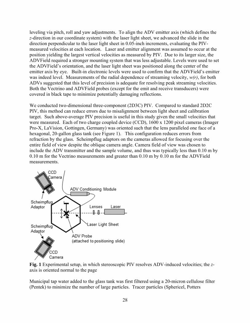
leveling vz-directiodirectionmeasuredposition yADVFielthe ADVemitter awas indeADVs suBoth the covered i We condPIV, thistarget. Swere meaPro-X, Lhexagonarefractionentire fieinclude th0.10 m fomeasurem

Fig. 1 Exaxis is or Municipa(Pentek)

via pitch, roon in our coon perpendiculd velocities ayielding the ld required a

VField’s orienxis by eye. ed level. M

uggested thatVectrino an

in black tape

ducted two-d method can

Such above-aasured. Each

LaVision, Goal, 20-gallonn by the glas

eld of view dhe ADV tranor the Vectriments.

xperimental riented norm

al tap water to minimize

ll and yaw aordinate systlar to the lasat each locatlargest verti

a stronger mntation, and Built-in eleeasurementst this level o

nd ADVFielde to minimiz

dimensional tn reduce erroaverage PIV h of two cha

ottingen, Gern glass tank (ss. Scheimpdespite the obnsmitter andino measurem

setup, in whmal to the pag

added to thee the number

adjustments. tem) with theser light sheetion. Laser ical velocitieounting systthe laser lig

ectronic levels of the radiaof precision id probes (excze potentially

three-compoors due to miprecision is

arge coupledrmany) was o(see Figure 1flug adaptorblique camer

d the sample ments and gr

hich stereoscge

e glass tank wr of large par

28

To align the laser light et in 0.05-incand emitter

es as measurtem that washt sheet wasls were usedal dependencis adequate fcept for the y damaging r

onent (2D3Cisalignment buseful in thi

d device (CCoriented suc1). This conrs on the camra angle. Cavolume, andreater than 0

opic PIV res

was first filterticles. Trac

he ADV emitsheet, we adch incremenalignment w

red by PIV. s less adjustas positioned d to confirm ce of streamifor resolvingemit and recreflections.

C) PIV. Combetween lighis study give

CD), 1600 x ch that the lennfiguration rmeras alloweamera field od thus was ty0.10 m by 0.

solves ADV

ered using a cer particles

tter axis (whdvanced the nts, evaluatinwas assumed

Due to its laable. Levels along the cethat the ADing velocity

g peak streamceive transdu

mpared to staht sheet and en the small 1200 pixel cns paralleledreduces errored for focusiof view was cypically less 10 m for the

V-induced vel

20-micron c(Sphericel, P

hich defines tslide in the

ng the PIV-d to occur at arger size, thwere used to

enter of the VField’s em, w(r), for bo

ming velocitiucers) were

andard 2D2Ccalibration velocities th

cameras (Imad one face ofrs from ing over the chosen to than 0.10 m

e ADVField

locities; the

cellulose filtPotters

the

the he o set

mitter oth ies.

C

hat ager f a

m by

z-

ter

29

Industries) with median diameter 11m were added to the filtered tap water resulting in a concentration on the order of 1 g m-3. The water was then mixed with a submersible pump. After allowing currents generated by the pump to decay, we recorded multiple sets of images while the ADV was operating in the tank. Before recording each set of images, we modified one or more user adjustable ADV settings and initiated ADV data collection. Then, after a delay of more than 15 seconds (the maximum acoustic streaming start up time reported in Kamakura, 1996), we recorded 341 images in single frame mode at 29.41 Hz using DaVis software (equivalent to a measurement duration of approximately 11.5 seconds). The maximum number of images that could be recorded in a single set was determined by the RAM capabilities of the hardware. Sets of images were also recorded with the ADV off (no ADV data collection) before most measurements of ADV-induced streaming in order to establish the level of background flow in the tank. We measured the flow induced by each ADV while systematically varying operating configurations. The Vectrino allows the duration, power and repetition frequency of its ultrasound pulses to be configured (Table 1). No other user configurable setting was observed to affect acoustic streaming. The duration of each ultrasound pulse is specified by the “transmit length” while the pulse repetition frequency is specified using the “nominal velocity range” setting. A larger nominal velocity range setting corresponds to a higher pulse repetition frequency and higher duty factor. The Vectrino configuration is reset to a default configuration (Table 1) each time the Vectrino software restarts. Only the ADVField’s pulse repetition frequency is typically adjusted, though it is possible to modify the pulse duration. There is no option to increase transmitted pulse power directly for the ADVfield. While testing the Vectrino, we held two of the three configurable settings that affect streaming velocity constant (at the level which caused the most acoustic streaming), while varying the remaining setting. We also varied multiple Vectrino settings at once. In total, we tested sixteen different combinations out of one hundred and twenty different possible combinations of settings. The combinations of Vectrino settings we investigated are those yielding the greatest variation in acoustic streaming velocity. As is typical in field operation, only the nominal velocity range setting on the ADVField was adjusted during imaging. Repeat tests of the Vectrino in the same configuration spaced months apart confirmed that neither ADV set up, temperature, seeding density nor other unknown factors substantially influenced streaming velocities. Table 1 ADV user selectable settings and their physical significance Setting name Physical

significance Available settings – Vectrino

Available settings – ADVField

Default settings - Vectrino

Nominal velocity range

Ultrasound pulse repetition frequency

+/-0.03, 0.10, 0.30, 1.00, 2.50, 4.00 ms-1

+/- 0.03, 0.10, 0.30, 1.00, 2.50 ms-1

0.30 ms-1

Transmit length

Pulse duration 0.3, 0.6, 1.2, 1.8, 2.4 mm

NA 1.8 mm

Power level Transmitted sound power

Low, Low+, High-, High

NA High

30

Velocity vector fields were computed from a timeseries of recorded images via stereoscopic cross-correlation in DaVis FlowMaster software. A multi-pass (or iterative) technique was used with an initial interrogation window size of 128 x 128 pixels or 64 x 64 pixels and a final interrogation window size of 32 x 32 pixels with 50% overlap between windows and Gaussian subwindow weighting. For the ADV configurations resulting in the slowest streaming velocities, computing vector fields from successive images (separated by 1/29 s) resulted in very small displacement (in pixels). In these cases, non-sequential images separated by up to 0.20 seconds were used. We imported vector field results to MATLAB for analysis of maximum streaming velocities, mean velocities in the sampling volume and along-beam velocity profiles. Measures of central tendency, computed over approximately 11.5 seconds (341 velocity fields), confirmed statistical convergence over the measurement period. The ADV sampling volume is an irregular shape defined by the intersection of the transmitted ultrasound beam and the receive beams. The sampling volume may be approximated as a 6-mm diameter circular cylinder for both the ADVField and the Vectrino (SonTek/YSI 2001; Nortek AS 2009). In contr ast, our stereoscopic PIV measured velocities in a plane cutting through the center of sample volume. Each velocity vector represented a spatial average over a rectangular interrogation window within this plane. To compare the velocity vector fields obtained through PIV with the velocities measured by the ADV itself, we computed a weighted average of the PIV measured velocity vectors falling within the ADV sampling volume. Each velocity vector was weighted according to the volume of the solid of revolution created by rotating the corresponding interrogation window about the sampling volume axis. The resulting estimates of sample volume average velocity (ws) approximate what the ADV itself measures with some uncertainty (because the exact shape of the sampling volume is unknown). Velocity measurement uncertainties were estimated from PIV data as the larger of a) the bootstrap 95% confidence interval and b) the inter-quartile range of vertical velocity over twelve PIV based background flow measurements. Results Both the Vectrino and the ADVField induced velocities that were primarily in the z-direction, i.e. parallel to the ADV emitter axis (e.g. Figure 2). The flow originated at the ultrasound emitter and increased with distance from the emitter, extending to the ADV sampling volume and beyond. Profiles of velocity along the centerline of the transmit beam, wr=0 (Figure 3, Figure 4) show that for both ADVs the velocity at the sample volume is close to the maximum velocity.

Fig. 2 Thladen, quvector fi The VectADVFielvelocitieslarge enoVariation2 in ordewith the nsetting). Wgeneratedwere obsmm (largtransmit velocities

he acoustic ouiescent waeld.

trino generatld generateds are aligned

ough to overwn of the acour of decreasinominal veloWith the nomd velocities aserved with tgest possiblelengths, noms. The smal

output of a ter as show

ted peak veld peak velocid with the axwhelm the fl

ustic streamining peak velocity range aminal velociapproximatethe followinge) and nominminal velocitlest Vectrino

Nortek Vecn in a CCD

ocities (wp) bities (wp) betxes of the ADflow signal inng velocity alocity. The gat +/- 2.50 mity range set ely 0.01 m s-

g Vectrino snal velocity rty ranges ando induced flo

31

ctrino induc camera im

between 0.0tween 0.009DVs’ ultrason some wetlaas a functiongreatest ADV

m s-1 (the largto the lowes

-1 lower. Thettings: powrange = +/- 4d power leveows (wp < 0.

ces a steady mage overlain

0005 m s-1 an5 m s-1 and 0

ound emittersand, boundan of ADV coVField inducgest availablst available v

he greatest Vwer level = hi4.0 m/s (largels resulted i.005 m s-1) o

flow in tracn by a PIV

nd 0.02 m s-1

0.02.2 m s-1.s (where r=0

ary layer, or bonfiguration ced velocitiele nominal vvalue, the A

Vectrino-induigh, transmit

gest possible)in slower acooccurred whe

cer-particlegenerated

1, while the . These peak0), and can bbackwater flis seen in T

es were obsevelocity rang

ADVField uced velocitit length = 2.). Smaller oustic streamen the power

e-

k be flows. able

erved ge

ies 4

m r

32

level was set to anything but “high” or when both the transmit length and nominal velocity range were reduced to their lowest level. Decreasing either the Vectrino’s nominal velocity range or transmit length in successive steps from the maximum to the minimum value produced a gradual monotonic decrease in the induced velocity (Figure 3a, Figure 3c). In contrast, adjusting the power level has a strong “step-function” type response: adjusting the power level from its highest to second highest setting (“high” to “high-“) drastically decreased peak velocities (from wp 0.02 m s-1 to wp 0.0025 m s-1) (Figure 3b). The ADVField behaved similarly to the Vectrino in response to reductions in nominal velocity range; induced velocities dropped by a fraction of each time the range was lowered (Figure 4). In general, the distance to the maximum streaming velocity from the ultrasound emitter increased with increasing nominal velocity range, increasing transmit length and increasing power level. Table 2 Flows induced by two ADV models for different ADV configurations as observed via PIV Nominal velocity range (m s-1)

Transmit length (mm)

Power level

Peak velocity wp (m s-1)*

Distance to peak velocity (mm below emitter)

Average velocity within ADV sampling volume ws (m s-1)*

Vectrino 4.00 2.40 High 0.0203 89 0.0101 1.00 2.40 High 0.0162 90 0.0088 2.50 2.40 High 0.0157 92 0.0094 4.00 1.20 High 0.0147 90 0.0081 0.30 2.40 High 0.0142 79 0.0072 0.30 1.80 High 0.0117 87 0.0063 0.10 2.40 High 0.0099 76 0.0054 0.03 2.40 High 0.0076 84 0.0044 4.00 0.30 High 0.0051 76 0.0029 0.03 1.20 High 0.0042 70 0.0026 4.00 2.40 High- 0.0024 84 0.0014 1.00 2.40 High- 0.0017 67 0.0013 4.00 2.40 Low+ 0.0009 82 0.0007 0.03 0.30 High 0.0009 55 0.0006 0.03 2.40 High- 0.0006 66 0.0004 4.00 2.40 Low 0.0005 37 0.0003 ADVField 2.50 NA NA 0.0227 84 0.0157 1.00 NA NA 0.0194 83 0.0129 0.30 NA NA 0.0132 76 0.0089 0.10 NA NA 0.0111 73 0.0071 0.03 NA NA 0.0095 74 0.0063 *Uncertainty intervals are 0.0003 m s-1 for the first configuration and 0.0001 m s-1 for all other configurations.

33

Fig. 3 Effect, as measured by PIV, of varying Vectrino transmit length, power and nominal velocity range. Profiles of Vectrino induced acoustic streaming velocity along the transmit beam centerline, wr=0 are shown for: a) different transmit lengths with nominal velocity range and power level constant at +/-4.0 m s-1 and “high”, respectively, b) different power levels with nominal velocity range and transmit length constant at +/-4.0 m s-1 and 2.4 mm, respectively and c) different nominal velocity ranges with transmit length and power level constant at 2.4 mm and “high”, respectively (Solid vertical lines show the approximate location of the sampling volume)

34

0 10 20 30 40 50 60 70 80 90 1000

0.005

0.01

0.015

0.02

0.025

c

wr=

0 (m

s−

1 )

Distance from ADV ultrasound emitter, z (mm)

+/−4.0 m/s+/−1.0 m/s+/−0.3 m/s+/−0.1 m/s+/−0.03 m/s

0 10 20 30 40 50 60 70 80 90 1000

0.005

0.01

0.015

0.02

0.025

a

wr=

0 (m

s−

1 )

2.4 mm1.2 mm0.3 mm

0 10 20 30 40 50 60 70 80 90 1000

0.005

0.01

0.015

0.02

0.025

b

wr=

0 (m

s−

1 )

HighHigh−Low+Low

35

Fig. 4 Effect of varying nominal velocity range with the SonTek ADVField. The profile of acoustic streaming velocity along the transmit beam centerline, wr=0, is shown for different nominal velocity ranges. (Solid vertical lines show the location of the sampling volume)

To understand the effect of acoustic streaming on the measurements reported by the ADV itself, the PIV data was used to compute the average velocity over the sampling volume ws. The values of ws are smaller than the peak velocities wp, but follow the same trends relative to ADV configuration. The maximum ws value was 0.0142 m s-1 for the ADVField and 0.0087 m s-1 for the Vectrino (Table 2). Sampling volume average velocities increase with increasing nominal velocity range for both the Vectrino and ADVField (Figure 5). The differences between ws and wp stem in part from the sampling volumes’ location with respect to peak induced flows (visible in Figures 3 and 4). The sample volume is fixed in space for each velocimeter, while the peak streaming location moves with configuration. The Vectrino’s sample volume is centered 50 mm from its emit transducer while the ADVField’s sample volume is centered 100 mm from its emit transducer. The Vectrino’s peak streaming occurs beyond its sample volume (ranging from 60 mm to 90 mm from the emit transducer). The ADVField’s peak velocity occurs between its sample volume and the ultrasound emitter (ranging from 70 to 90 mm from the emitter).

0 10 20 30 40 50 60 70 80 90 100 1100

0.005

0.01

0.015

0.02

0.025

Distance from ADV ultrasound emitter, z (mm)

wr=

0 (m

s−

1 )

+/−2.5 m/s+/−1.0 m/s+/−0.3 m/s+/−0.1 m/s+/−0.03 m/s

36

Fig. 5 Volume averaged acoustic streaming velocity in the ADV sampling volumes, ws, as measured by PIV The differences between ws and wp are also related to the variation of the velocity in the direction perpendicular to the transmit beam, w(r). At the center of the sampling volume, radial profiles of axial velocity approximate Gaussian curves (Figure 6), with widths () of 2.5 mm and 3.5 mm for the Vectrino and ADVField, respectively. As a result, the acoustic streaming velocity decreases significantly from the centerline to the edge of the sampling volume, thus ws < wp.

0 0.5 1 1.5 2 2.5 3 3.5 40

0.002

0.004

0.006

0.008

0.01

0.012

0.014

0.016

0.018

0.02

Representative error bar

ws (

m s

−1 )

Nominal Velocity Range (m s−1)

VectrinoADVField

37

Fig. 6 Radial distribution of acoustic streaming velocities w(r) for two ADV models at the vertical midpoint of their respective sampling volumes (radial extent of sample volumes shown as black vertical lines). The settings generating maximum streaming velocities were selected for both velocimeters. FWHM stands for full width at half maximum. For all ADV configurations, radial velocities were generally an order of magnitude or more lower than vertical velocities and of the same order as background velocities. Image sets recorded with the ADV off were made just before most image sets of ADV induced acoustic streaming (twelve image sets in total, each with 11.5 second duration). From these images, we measured background vertical velocities as high as 0.004 m s-1. Typically background flow was much lower. The inter-quartile range of background vertical velocities, computed across the twelve image sets, averaged 0.00012 m s-1 over the field of view. The inter-quartile ranges for horizontal velocities were of similar magnitude. By comparing sample-volume average vertical velocities, ws, with velocity data collected by the Vectrino, we determine that for certain combinations of user-selectable settings the Vectrino accurately measures the flow it induces. At high power, for nominal velocity ranges of +/-1.0 m/s or less, the Nortek Vectrino measured velocities that were statistically equivalent to PIV-based measurements (ws) or within 20% of the PIV-based measurements (Figure 7). Self-measurement was not effective when the ADV was operated at lower power levels or at higher nominal velocity ranges. When operated in these configurations, the Vectrino reported median velocity measurements of approximately 0 m s-1, with signal to noise ratios lower than 10 dB in all but one case. Self-measurement of the Vectrino induced flow failed only when the SNR was substantially lower than 10 dB or the nominal velocity range setting was inappropriate (i.e. far greater than the range of observed velocities). The SonTek ADVField collected valid measurements of the flow it induced regardless of the nominal velocity range setting. Self-measured flows were for all configurations within 50% of the PIV-based flow measurements. The discrepancies in the measurements were greatest for the two largest nominal velocity ranges

−30 −20 −10 0 10 20 30−0.01

−0.005

0

0.005

0.01

0.015

0.02

0.025

Distance from ADV emitter center (mm)

Med

ian

velo

city

(m

s−

1 )

← FWHM =8.3 mmσ =3.5 mm

← FWHM =5.8 mmσ =2.5 mm

Measured profile ADVFieldGaussian fit ADVFieldMeasured profile VectrinoGaussian fit Vectrino

38

(Figure 8). Interestingly, the Nortek Vectrino self-measurements were consistently higher than PIV values, while SonTek ADVField self-measurements were consistently lower than PIV values. The ADVs’ self-measurements could differ from the PIV values because our calculation of ws does not recreate the complex spatial averaging scheme used by the ADVs. When acoustic backscatter is of low strength, the Vectrino weights each localized velocity measurement (due to a single tracer particle) by the return signal strength (Atle Lohrmann, personal communication, 8/10/2010). When the backscattered signals are very strong, velocity data from all tracer particles in the sample volume are weighted equally. Thus there is a continuum of spatial weighting functions that depend on particle type, particle loading, and ADV power level. Our PIV based estimates of sample volume velocity, ws, use the simplest weighting scheme, i.e. a direct volume average corresponding to the case of large backscatter amplitude.

Fig. 7 Simultaneous ADV (Nortek Vectrino) and PIV measurements of Vectrino induced acoustic streaming over its sampling volume, ws, for different combinations of transmit length and nominal velocity range at high power

0

0.002

0.004

0.006

0.008

0.01

0.012

0.3,0.03 1.2,0.03 2.4,0.03 2.4,0.1 1.8,0.3 2.4,0.3 2.4,1.0

Transmit Length (mm),Nominal Velocity Range (m s−1)

ws (

m s

−1 )

ADVPIV

39

Fig. 8 Simultaneous ADV (SonTek ADVField) and PIV measurements of ADVField induced acoustic streaming over the sampling volume, ws, for different ADVField nominal velocity ranges Discussion Profiles of ADV induced flow along the transmit beam axis (wr=0) (Figure 3, Figure 4) show the same features described in existing analytical models of acoustic streaming. These analytical solutions indicate acoustic streaming velocity increases with distance from the sound source (Wu and Du 1993; Riley 2000). The observed flow increased with distance from the ADV emitter before peaking and beginning to decline at a distance between 30 and 90 mm. Mitome et al. (1995) predicted such behavior, attributing it to momentum transport away from the ultrasound beam axis. The radial velocity distribution (Figure 6) also agrees with theoretical derivations of acoustic streaming velocity, which assume Gaussian profiles (Lighthill 1978). Analytical solutions derived from equations 1-3 predict that the magnitude of acoustic streaming varies either with transmitted sound amplitude, a, or with a2 (Nyborg 1998; Mitome 1995; Wu and Du 1993). Our data suggest a dependence on a2. We found a linear relationship between wp and ADV time-average power consumption for both the Vectrino and the ADVField (see Figure 9). Power consumption data were collected with a wattmeter (Kill A Watt, P3 International) (Vectrino) or obtained from the operating manual (ADVField). For the Vectrino, time average power consumption, Pc, was measured while varying the user-selectable power level at maximum transmit length and nominal velocity range. The ADVField’s transmitted power is not directly user-adjustable, and thus the power usage data are less conclusive, as discussed further below. Additional support for the Vectrino’s apparent linear relationship between transmitted sound power and acoustic streaming can be seen in the variation of transmitted sound intensity

0.03 0.10 0.30 1.0 2.50

0.002

0.004

0.006

0.008

0.01

0.012

0.014

0.016

Nominal Velocity Range (m s−1)

ws (

m s

−1 )

ADVPIV

40

with power level setting (Table 3). When the transmit length and nominal velocity range settings are maximized, the highest Vectrino power level corresponds to time-average sound intensity of approximately 168 dB (referenced to 1 microPascal at 1 meter) (Atle Lohrmann, personal communication, 7/14/2009). For continuous sound transmission from a 6-mm diameter transducer through water, this intensity corresponds to a sound amplitude of 170 kPa. The difference between successively lower power levels is approximately 6 dB (Atle Lohrmann, personal communication, 7/14/2009) indicating that the minimum power level corresponds to a time-average intensity of approximately 150 dB and an amplitude of 21kPa (for continuous sound). Sound amplitudes computed from these intensity values (assuming continuous sound and the reference pressure), show a clear quadratic relationship with wp (R

2 = 0.99). These results also suggest that peak acoustic streaming velocity wp varies directly with sound power and hence sound amplitude squared (a2) not a. While the sound amplitudes calculated from time-average intensity hold for continuous sound, the sound amplitudes for different power level settings would increase by the same factor for pulsed sound. Hence the percent differences are correct even if the sound amplitudes are underestimated. When evaluating models with this data, it is important to consider that non-linear sound propagation, which increases with amplitude, may obscure the relationship between amplitude and streaming velocity. Specifically, non-linear ultrasound propagation, not accounted for in equation (2), transfers energy from the fundamental frequency to harmonics, which are more rapidly absorbed and thus magnify acoustic streaming at higher power levels (Wu and Du 1993).

Fig. 9 Relationship between ADV time average power consumption and peak acoustic streaming velocity, wp. Vectrino time average power consumption was varied by adjusting the power level setting. ADVField time average power consumption was varied by adjusting the only setting typically adjusted: the nominal velocity range

3 3.5 4 4.5 5 5.50

0.005

0.01

0.015

0.02

0.025

Time−average power consumption (W)

wp (

m s

−1 )

VectrinoADVField

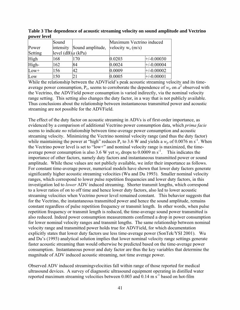
41

Table 3 The dependence of acoustic streaming velocity on sound amplitude and Vectrino power level

Power Setting

Sound intensity level (dB)

Sound amplitude, a (kPa)

Maximum Vectrino induced velocity ws (m/s)

High 168 170 0.0203 +/-0.00030 High- 162 84 0.0024 +/-0.00004 Low+ 156 42 0.0009 +/-0.00002 Low 150 21 0.0005 +/-0.00001 While the relationship between the ADVField’s peak acoustic streaming velocity and its time-average power consumption, Pc, seems to corroborate the dependence of wp on a2 observed with the Vectrino, the ADVField power consumption is varied indirectly, via the nominal velocity range setting. This setting also changes the duty factor, in a way that is not publicly available. Thus conclusions about the relationship between instantaneous transmitted power and acoustic streaming are not possible for the ADVField. The effect of the duty factor on acoustic streaming in ADVs is of first-order importance, as evidenced by a comparison of additional Vectrino power consumption data, which prima facie seems to indicate no relationship between time-average power consumption and acoustic streaming velocity. Minimizing the Vectrino nominal velocity range (and thus the duty factor) while maintaining the power at “high” reduces Pc to 3.6 W and yields a wp of 0.0076 m s-1. When the Vectrino power level is set to “low+” and nominal velocity range is maximized, the time-average power consumption is also 3.6 W yet wp drops to 0.0009 m s-1. This indicates the importance of other factors, namely duty factors and instantaneous transmitted power or sound amplitude. While these values are not publicly available, we infer their importance as follows. For constant time-average power, numerical models have shown that lower duty factors generate significantly higher acoustic streaming velocities (Wu and Du 1993). Smaller nominal velocity ranges, which correspond to lower pulse repetition frequencies and lower duty factors, in this investigation led to lower ADV induced streaming. Shorter transmit lengths, which correspond to a lower ratios of on to off time and hence lower duty factors, also led to lower acoustic streaming velocities when Vectrino power level remained constant. This behavior suggests that for the Vectrino, the instantaneous transmitted power and hence the sound amplitude, remains constant regardless of pulse repetition frequency or transmit length. In other words, when pulse repetition frequency or transmit length is reduced, the time-average sound power transmitted is also reduced. Indeed power consumption measurements confirmed a drop in power consumption for lower nominal velocity ranges and transmit lengths. The same relationship between nominal velocity range and transmitted power holds true for ADVField, for which documentation explicitly states that lower duty factors use less time-average power (SonTek/YSI 2001). Wu and Du’s (1993) analytical solution implies that lower nominal velocity range settings generate faster acoustic streaming than would otherwise be predicted based on the time-average power consumption. Instantaneous power and duty factor are thus the key variables that determine the magnitude of ADV induced acoustic streaming, not time average power. Observed ADV induced streamingvelocities fall within range of those reported for medical ultrasound devices. A survey of diagnostic ultrasound equipment operating in distilled water reported maximum streaming velocities between 0.003 and 0.14 m s-1 based on hot-film

42

anemometry measurements (Starritt et al. 1989). A PIV-based study of ultrasonic lithotripters found axial streaming velocities up to 0.03 m s-1 and radial velocities up to 0.01 m s-1 (Choi et al. 2004). Another PIV study examined a 3.3 MHz medical ultrasound device operating in continuous mode, observing maximum axial velocities of either 0.06 m s-1 or 0.008 m s-1 depending on the power setting selected (Cosgrove et al. 2001). Hartley (1995) tested a first generation ADV with adjustable sampling volume location and adjustable operating frequency in quiescent fluid (both water and blood) using the ADV itself. He reported sample-volume average acoustic streaming velocities (ws) no greater than 0.01 m s-1. The higher operating frequency (20 MHz) induced faster acoustic streaming than the lower operating frequency (10 MHz). A non-linear relationship between pulse repetition frequency and maximum streaming velocity was also observed. When evaluating ADVs’ self-measurement of acoustic streaming velocities (Figure 7, Figure 8), the disagreement between PIV and ADV data is particularly large at high nominal velocity settings. Use of higher nominal velocity ranges leads to higher ADV sampling error (McLelland and Nicolas 2000), and likely contributed to the greater disagreement at these ranges. Discrepancies between simultaneous ADV and PIV measurements may also be due the complex shape of the sampling volume, which was here approximated as a circular cylinder of diameter 6 mm for both ADVs. The general conclusion of this work is that ADV induced acoustic streaming can bias ADV measurements depending on the ADV configuration used. Our experiments in quiescent conditions do not, however, resolve the effect of ADV induced flow on measurements in non-quiescent conditions. The nature of the ambient flow may influence the structure of the ADV acoustic stream, and thus the way in which it affects measurements. We briefly consider two classes of ambient flow: unidirectional flow perpendicular to the ADV axis (“cross-flow”), and homogeneous isotropic turbulence with no mean flow. A cross-flow will advect the axial momentum away from the ADV emitter axis and sampling volume, potentially reducing the bias in ADV measurements. The measurements of Snyder and Castro (1999) showed ADV-measured ws values were “substantially reduced” in the presence of a cross-flow of magnitude 0.009 m/s when the ADV nominal velocity range was set to 0.03 m/s (compared to a peak ws of 0.007 m/s in quiescent conditions). The streaming was reported to be absent at cross-flows of 0.02 m/s or above. Counter to this line of reasoning, we note that successful ADV operation relies on the scattering of the emitted sound in the sampling volume. When emitted pulses continue to reach the sampling volume before being advected away (as required for accurate measurement), the spatial gradient created by sound absorption may continue to induce steady streaming. Consequently, we conjecture that cross flow reduces but does not eliminate the ADV induced acoustic streaming. To evaluate this, the effects of acoustic streaming would need to be separated from the effects of the ADV wake. The cross-flow velocity range between 0 and 0.02m/s remains to be studied, and is important for cases such as wetlands and river backwaters. To determine the effect of turbulence on acoustic streaming, we examined ADV and PIV data collected in an experiment that was performed to characterize a stirred turbulence tank (Variano and Cowen 2008). This apparatus had RMS turbulent velocities of approximately 0.04 m/s, with

43

mean flows less than 0.005 m/s. The data on mean velocities show strong evidence that acoustic streaming exists and influences the ADV measurements despite the turbulent shearing motions (Figure 10). The statistically stationary flow was measured with a Nortek Vectrino ADV, and then by PIV (with the ADV probe removed). The ADV probe was mounted in two orientations: first with the ultrasound emitter axis oriented towards the negative z-direction (tank coordinates) and then with emitter axis oriented towards the positive x-direction. Comparing the three measurements suggests that ADV induces a velocity of roughly 0.002 m/s in the direction parallel to the emitter axis. That is, PIV and ADV measurements agree in any direction other than the ADV’s axial direction, and the ADV velocities shift when the orientation is shifted. The turbulence is nearly isotropic and the mean flows small, thus we expect that the effect is not due to altered ADV wakes. While noise levels in ADV measured axial velocities differ from noise levels in the radial velocities due to probe geometry, this phenomenon does not affect mean flow measurements (Voulgaris and Trowbridge, 1998). The apparent effect of acoustic streaming on the sample-volume average flow velocity is roughly 25% of that which we would expect in a quiescent flow, where a Vectrino with the same settings (Nominal velocity range = +/-1.00 m/s, Transmit length =2.4 mm, Power Level = High) would produce a ws of approximately 0.008 m/s (see Figure 5). This persistence of acoustic streaming despite strong turbulent shear lends some support to our hypothesis that acoustic streaming will persist in a cross-flow. In this respect, it is also of interest to note that there is indeed a cross-flow (albeit a weak one) in this data.

Fig. 10 Time-averaged mean velocities in a turbulent stirred tank as measured by PIV and an ADV oriented in two different directions. Discrepancies between measurements suggest that acoustic streaming persists and biases ADV measurements despite turbulent flow and cross-flow

-0.2

-0.1

0

0.1

0.2

0.3

0.4

0.5

0.6

<u> <v> <w>

Tim

e av

erag

e ve

loci

ty (

cm s

-1)

Velocity component

ADV points in -z

ADV points in +x

PIV

ADV ADV ADV ADV ADV ADVPIV PIV

44

The extent to which ADV acoustic streaming affects ADV data quality depends on a combination of four factors (1) the internal (non-adjustable) ADV specifications, (2) user-selected configuration, (3) ambient conditions, and (4) the velocity statistics of interest. The internal ADV specifications that influence how acoustic streaming impacts measurement are the ultrasound frequency and the location of the sampling volume. Devices using higher frequency ultrasound such as the SonTek 16-Mhz ADVOcean are expected to generate higher streaming velocities. The user-adjustable range of time-average transmitted power levels and duty factors will determine the extent and pattern of streaming, though the user’s range of choices are typically restricted by other demands of the measurement. That is, the user’s selection of a nominal velocity range is typically governed by the expected flow conditions, while selection of the power level and transmit length are governed by particle density in the flow. Ambient conditions affecting streaming velocity include cross-flow velocity and turbulence, although the interaction between these and acoustic streaming is not yet well characterized. Temperature and particle density will likely affect the streaming velocities since they influence ultrasound absorption, the primary driving force behind acoustic streaming. In pure water, sound attenuation decreases with increasing temperature (up to 74 degrees Celsius) (Kuttruff 1991), and thus we expect larger acoustic streaming at colder temperatures. The shape of suspended solids (Hay 1991) and the concentration and composition of dissolved substances also affect ultrasound absorption (Kuttruff 1991); the effect of these factors on acoustic streaming may be of great importance to studies that use ADVs to measure sediment fluxes. While the user typically has few options for changing the above three factors, they may have control over the orientation of the velocimeter probe. By carefully choosing the ADV orientation with respect to the velocity statistics of interest, one can reduce the significance of acoustic streaming for flow measurements. The very low radial velocities measured here and in most observational studies of ultrasound induced streaming suggest that measurement of velocity components perpendicular to the ADV emitter axis are negligibly impacted (higher order statistics such as Reynolds’ stresses may be affected). Thus to minimize bias from acoustic streaming, the ADV’s emitter axis should be aligned perpendicular to the flow direction of greatest interest. Unfortunately, due to the geometry of the probe, the component of velocity parallel to the emitter axis is the one most precisely measured by the ADV (SonTek, 1997). Measurements of velocities parallel to the emitter axis also exhibit many times less noise than measurements of velocities perpendicular to the emitter axis (Lohrmann et al. 1994; Nikora and Goring 1998; Cea et al. 2007). Hence, as far as ADV probe orientation, there is a tradeoff between precision and accuracy in cases where acoustic streaming is non-negligible. If the experimental details cannot be altered to eliminate the bias due to acoustic streaming, the magnitude of the bias should be quantified as best as possible. The simplest way to quantify acoustic streaming bias is to use values reported here for ws, with the important caveat that different water quality parameters, flows, and ADV specifications can cause significant differences in acoustic streaming velocities. Vectrino measurements were collected at 24 degrees C and ADVField measurements at 21 degrees C. The loading of the 11-micron glass spheres used as PIV tracer particles (estimated to be 1 mg L-1) was optimized for PIV. Alternative options for estimating the induced flow include (in approximate order of increasing cost and difficulty) measuring streaming in a quiescent water sample with the ADV itself,

45

comparing velocity statistics for different ADV orientations, predicting streaming velocity via analytical or numerical models (e.g. Wu and Du 1993; Kamakura et al. 1996) or measuring streaming directly with an alternate flow measurement technology. The flow chart in Figure 11 organizes the results of our analysis to help ADV users identify whether acoustic streaming bias is significant for a particular application and, if so, choose an option for characterizing the bias. Common environmental flows in which acoustic streaming may represent a significant source of bias include wetlands, river backwaters, sedimentation tanks and tidal flows near slack tide. In low-flow situations such as these, acoustic streaming bias is likely outside manufacturer specified error bounds of 0.5% of the measured value or +/-1 mm s-1 for the Vectrino (Nortek AS 2009) and 1% of the measured velocity or +/-0.25 cm s-1 for the ADVField (SonTek 1997) (Table 4). Table 4 The error due to acoustic streaming as a percentage of measured velocity for different nominal velocity ranges. Percent error values are based on the assumption the nominal velocity range is chosen for optimal measurement of vertical velocity Nominal velocity range

Vertical velocity range (the maximum vertical velocity optimally measured in this nominal. velocity range)

Minimum vertical velocity optimally measured at this nominal velocity range

Sample volume average acoustic streaming velocity, ws

Minimum acoustic streaming error

Maximum acoustic streaming error

m s-1 m s-1 m s-1 m s-1 Vectrino 0.03 0.08 NA 0.0044 5.5% >5.5% 0.10 0.13 0.08 0.0054 4.2% 6.8% 0.3 0.27 0.13 0.0072 2.7% 5.5% 1.0 0.54 0.27 0.0088 1.6% 3.3% 2.5 0.94 0.54 0.0094 0.99% 1.7% 4.0 1.5 0.94 0.010 0.68% 1.1% ADVField 0.03 0.08 NA 0.0063 7.9% >7.9% 0.10 0.15 0.08 0.0071 4.7% 8.9% 0.30 0.3 0.15 0.0089 3.0% 5.9% 1.0 0.75 0.3 0.013 1.7% 4.3% 2.5 0.9 0.75 0.016 1.7% 2.1%

Fig. 11 Aselecting Conclusi In quiescinduce acsamplingthe ultrasfrom the between transmittwith the utransmit If ambienacoustic by acouslow flow

A flow chart g an option fo

ions

cent water, thcoustic streag volume. Thsound emitteemitter. Anthe two ADV

ted ultrasounuser-adjustalength and n

nt flow velocstreaming mtic streaming

ws. The effec

for identifyior characteri

he SonTek 1aming along he flow is pr

er before reanalytical moVs suggest s

nd power andable power lenominal velo

cities are of may represen

g are those oct is present,

ing when acoizing acousti

0-MHz ADVthe transmitrimarily in thching a peak

odels for acostreaming ved the duty faevel setting (ocity range s

the order of nt a significanof velocity co though of le

46

oustic streamic streaming

VField and tt beam, therehe axial direk as high as 0ustic stream

elocities are pactor. Peak(Vectrino onettings (both

f potential acnt source of omponents aesser magnit

ming may big velocity in

the Nortek Veby altering tection and in0.02 m s-1 at

ming from theproportionalinstantaneou

nly) and dutyh ADVs).

coustic streambias. Measu

aligned withtude, in turb

ias ADV methese situati

Vectrino werthe velocity

ncreases witht a distance oe literature al to the peakus transmittey factor depe

ming velociturements mo

h the ADV emulent flows

asurements ions

re observed twithin the

h distance froof 0.06 to 0.

and a compark instantaneoed power varends on both

ties, then ost likely biamitter axis inand cross-flo

and

to

om 09 m rison

ous ries

h the

ased n ows.

47

A range of options exists for accounting for streaming when it is unavoidable, including measurement of streaming magnitudes with the ADV itself and analytical or numerical modeling. We evaluate the quality with which the ADVs measure the acoustic streaming they induce, finding ADV measurements agree to within 20% percent when the velocity settings are appropriate for the streaming magnitude in question. Analytic models for acoustic streaming describe the general form of the ADVs well, although special consideration is necessary due to the pulsed nature of ADVs’ ultrasound transmission. The measurements presented here are used to guide the application and refinement of the existing models to more accurately describe ADVs. References Cea L, Puertas J, Pena L (2007) Velocity measurements on highly turbulent free surface flow using ADV. Exp Fluids 42: 333-348 Choi MJ, Doh DH, Cho CH, Kang KS, Paeng DG, et al. (2004) Visualization of acoustic streaming produced by lithotripsy field using a PIV method. J Phys Conference Series 1:217-223 Cosgrove JA, Buick JM, Pye SD, Greated CA (2001) PIV applied to Eckart streaming produced by a medical ultrasound transducer. Ultrasonics 39:461-464 Elgar S, Raubenheimer B, Guza RT (2005) Quality control of acoustic Doppler velocimeter data in the surfzone. Meas Sci Technol 16:1889-1893 Faraday M (1831) Acoustic streaming. Philos Trans R Soc Lond 121:299-340 Hartley CJ (1995) Doppler measurement of acoustic streaming. In: Proceedings of the 1995 IEEE Ultrasonics Symposium, IEEE Publishing, pp. 1537-1540. Hay AE (1991) Sound scattering from a particle-laden, turbulent jet. J Acoust Soc Am 90:2055-2074 Kamakura T, Sudo T, Matsuda K, Kumamoto Y (1996) Time evolution of acoustic streaming from a planar ultrasound source. J Acoust Soc Am 100:132-138 Kaye GWC, Laby TH (1986) Tables of physical and chemical constants. Longman, New York Kumar A, Gogate PR, Pandit AB (2007) Mapping of acoustic streaming in sonochemical reactors. Ind Eng Chem Res 46:4368-4373 Kuttruff H (1991) Ultrasonics: Fundamentals and applications. Elsevier Applied Science, New York Lacy JR, Sherwood CR (2004) Accuracy of a pulse-coherent acoustic Doppler profiler in a wave-dominated flow. J Atmospheric Ocean Technol 21:1448-1461

48

Lhermitte R, Serafin R (1984) Pulse-to-pulse coherent Doppler sonar signal processing techniques. J Atmos Ocean Technol 1: 293–308 Lighthill J (1978) Acoustic streaming. J Sound Vib 61:391-418 Lohrmann A, Cabrera R, Kraus NC (1994) Acoustic-Doppler velocimeter (ADV) for laboratory use. In: Fundamentals and Advancements in Hydraulic Measurements and Experimentation Proceedings, Buffalo, NY, ASCE publications, pp. 351–365. Makarov S, Semenova N, Smirnov V (1989) Acoustic streaming model for an intense sound beam in free space. Fluid Dyn 24:823-826 McLelland SJ, Nicholas AP (2000) A new method for evaluating errors in high-frequency ADV measurements. Hydrol Process 14:351-366 Mitome H, Kozuka T, Tuziuti, T (1995) Effects of nonlinearity in development of acoustic streaming. Jpn J Appl Phys 34:2584-2589 Nepf HM (1999) Drag, turbulence, and diffusion in flow through emergent vegetation. Water Resour Res 35:479-89 Nikora VI, Goring DG (1998) ADV measurements of turbulence: can we improve their interpretation? J Hydraul Eng 124(6): 630-634 Nortek AS (2009) Vectrino velocimeter. Nortek AS, Norway Nyborg WL (1998) Acoustic streaming. In Nonlinear Acoustics, eds. MF Hamilton, DT Blackstock, Academic Press, Chestnut Hill, MA Riley N (2001) Steady streaming. Annu Rev Fluid Mech 33:43-65 Riley N (1997) Acoustic streaming. In: Encyclopedia of Acoustics, ed. MJ Crocker, John Wiley & Sons, New York Snyder WH, Castro IP (1999) Acoustic Doppler velocimeter evaluation in stratified towing tank. J Hydraul Eng 125:595-603 Starritt H, Duck F, Humphrey V (1989) An experimental investigation of streaming in pulsed diagnostic ultrasound beams. Ultrasound Med Biol 15:363-373 SonTek (1997) Acoustic Doppler Velocimeter (ADV) principles of operation. SonTek, San Diego SonTek/YSI (2001) ADVField operation manual. SonTek/YSI, San Diego

49

Variano EA, Cowen EA (2008) A random-jet-stirred turbulence tank. J Fluid Mech 604:1-32 Voulgaris G, Trowbridge JH (1998) Evaluation of the acoustic Doppler velocimeter (ADV) for turbulence measurements. J Atmospheric Ocean Technol 15:272-289 Wu J, Du G (1993) Acoustic streaming generated by a focused Gaussian beam and finite amplitude tonebursts. Ultrasound Med Biol 19:167-176

50

Chapter 4 Gas exchange in wetlands with emergent vegetation: the effects of wind and thermal convection at the air-water interface 1. Motivation Gas fluxes between wetlands and the atmosphere are an essential component of global and local biogeochemical cycling. Wetlands affect the global balance of the greenhouse gas methane, emitting more methane than any other source [Denman et al., 2007]. Wetlands are also net sinks of atmospheric carbon dioxide, thus their impact on global radiative forcing depends on the molar ratio of carbon sequestered to methane emitted [Brix et al., 2001; Whiting and Chanton, 2001]. Locally, wetlands are major sources of toxic methyl mercury to freshwater environments [Rudd, 1995] and evasion of volatile mercury species to the atmosphere is an important component of wetland mercury budgets [Selvendiran et al., 2008]. Within individual wetlands, oxygen transport from the atmosphere into the water column influences a wide variety of chemical and biological processes. Gas transfer in wetlands can occur via three pathways: the gas-filled tissue or aerenchyma of emergent vegetation, bubbles rising from the substrate to the water surface (ebullition), and hydrodynamic transport of dissolved gas through the surface water. Our focus is on the last of these. While the other pathways may dominate at times, hydrodynamic gas transport is particularly important when emergent vegetation is senescent; it also acts indirectly as a control on the formation of bubbles. Hydrodynamic gas transport has received notably little study so far, and we present below the first detailed mechanistic exploration of this pathway in wetlands. A central goal is to help those evaluating wetland greenhouse gas fluxes, either via biogeochemical models or observation, accurately capture hydrodynamically driven gas fluxes. 2. Background The limiting step for the air-water exchange of sparingly soluble gases like carbon dioxide, methane, elemental mercury and oxygen occurs on the waterside of the air-water interface [Liss and Slater, 1974]. When the water column is well mixed, the interfacial exchange is controlled in the uppermost region of the surface water, since stirring is attenuated near the water surface, In such cases, an approximation is possible in which gas flux (J) across the air-water interface can often be modeled as the product of a gas transfer velocity (k) and the difference between the dissolved gas concentration in the bulk of the water column (C) and the concentration at the water surface (Ceq), which is in equilibrium with the air above (equation 1). The concentration in equilibrium with the air above is equal to the concentration in the air multiplied by the Ostwald solubiliy.

CCkJ eq (1)

The gas transfer velocity k is a measure of the near-surface stirring in the water that drives exchange of sparingly soluble gases across the air-water interface. As we will show later, this model is appropriate even in wetlands with relatively slow-moving water. In addition to stirring,

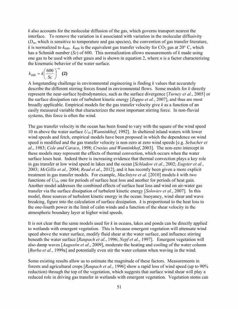
51

k also accounts for the molecular diffusion of the gas, which governs transport nearest the interface. To remove the variation in k associated with variation in the molecular diffusivity (Dm, which is sensitive to temperature and gas species), the convention of gas transfer literature, k is normalized to k600. k600 is the equivalent gas transfer velocity for CO2 gas at 20 C, which has a Schmidt number (Sc) of 600. This normalization allows measurements of k made using one gas to be used with other gases and is shown in equation 2, where n is a factor characterizing the kinematic behavior of the water surface.

n

Sckk

600600 (2)

A longstanding challenge in environmental engineering is finding k values that accurately describe the different stirring forces found in environmental flows. Some models for k directly represent the near-surface hydrodynamics, such as the surface divergence [Turney et al., 2005] or the surface dissipation rate of turbulent kinetic energy [Zappa et al., 2007], and thus are most broadly applicable. Empirical models for the gas transfer velocity give k as a function of an easily measured variable that characterizes the most important stirring force. In non-fluvial systems, this force is often the wind. The gas transfer velocity in the ocean has been found to vary with the square of the wind speed 10 m above the water surface U10 [Wanninkhof, 1992]. In sheltered inland waters with lower wind speeds and fetch, empirical models have been proposed in which the dependence on wind speed is modified and the gas transfer velocity is non-zero at zero wind speeds [e.g. Sebacher et al., 1983; Cole and Caraco, 1998; Crusius and Wanninkhof, 2003]. The non-zero intercept in these models may represent the effects of thermal convection, which occurs when the water surface loses heat. Indeed there is increasing evidence that thermal convection plays a key role in gas transfer at low wind speed in lakes and the ocean [Schladow et al., 2002; Eugster et al., 2003; McGillis et al., 2004; Read et al., 2012], and it has recently been given a more explicit treatment in gas transfer models. For example, MacIntyre et al. [2010] models k with two functions of U10, one for periods of surface heat loss and another for periods of heat gain. Another model addresses the combined effects of surface heat loss and wind on air-water gas transfer via the surface dissipation of turbulent kinetic energy [Soloviev et al., 2007]. In this model, three sources of turbulent kinetic energy in the ocean: buoyancy, wind shear and wave breaking, figure into the calculation of surface dissipation. k is proportional to the heat loss to the one-fourth power in the limit of calm winds and a function of the shear velocity in the atmospheric boundary layer at higher wind speeds. It is not clear that the same models used for k in oceans, lakes and ponds can be directly applied to wetlands with emergent vegetation. This is because emergent vegetation will attenuate wind speed above the water surface, modify fluid shear at the water surface, and influence stirring beneath the water surface [Raupach et al., 1996; Nepf et al., 1997]. Emergent vegetation will also damp waves [Augustin et al., 2009], moderate the heating and cooling of the water column [Burba et al., 1999a] and potentially even stir the water column when waving in the wind. Some existing results allow us to estimate the magnitude of these factors. Measurements in forests and agricultural crops [Raupach et al., 1996] show a rapid loss of wind speed (up to 90% reduction) through the top of the vegetation, which suggests that surface wind shear will play a reduced role in driving gas transfer in wetlands with emergent vegetation. Vegetation stems can

52

contribute to turbulent kinetic energy through wake production [Nepf et al., 1997]. Nighttime heat losses in open water can exceed heat losses in emergent vegetation by a factor of five [Burba et al., 1999a], which raises the possibility that thermal convection and resulting gas transfer may also be less intense in wetlands than in areas of open water. There are few data sets to test these hypotheses or predict k for wetlands specifically [Kadlec and Wallace, 2009; Kadlec and Knight, 1996]. With insufficient data for general predictions, researchers have taken several approaches to estimate dissolved gas fluxes in wetlands. Some wetland studies have relied on the relationships for k derived from ocean, lake and river experiments [Zhang et al., 2006; Matthews et al., 2003; Spieles and Mitsch, 2003; Lindberg and Zhang, 2000; Barber et al., 1988]. Others have used small, constant values for k [Maltais-Landry et al., 2009; Tian et al., 2010]. Some wetland models disregard the flux of dissolved gas across the air-water interface entirely, arguing that the other gas transport pathways dominate wetland gas fluxes, effectively setting k = 0. In these m odels, methane transport through the wetland water column is modeled to occur only through plant-mediated transfer or ebullition [e.g. Li et al., 2010; Walter and Heimann, 2000; Potter, 1997]. Oxygen transport through the wetland water column, which is important in quantifying aerobic oxidation of methane, is modeled to occur only through plant-mediated transfer [e.g. Cao et al., 1996; Zhuang et al., 2002]. Other models treat any standing water in wetlands similarly to the saturated zone of the soil, where molecular diffusivity alone governs the flux of dissolved gas [Zhuang et al., 2004; Riley et al., 2011].The handful of gas transfer velocity measurements that have been made in wetlands with emergent vegetation show that k values are an order of magnitude lower than those commonly measured in the ocean, lakes or rivers. Specifically, floating chamber measurements in a Florida hardwood swamp indicated that k600 averaged 0.78+/-0.54 cm hr-1 [Happell et al., 1995] and SF6 tracer releases in the patterned marshes of the Florida Everglades indicated k600 there ranged from 0.3 to 1.8 cm hr-1 [Variano et al., 2009]. While these observed values in wetlands are quite low, they are still too large to represent the effects of molecular diffusion alone (which can by quantified from the numerical solution to the diffusion equation and the molecular diffusivity). Since gas transfer velocities in wetlands with emergent vegetation differ from those in other aquatic environments, and emergent vegetation modifies the common drivers of gas transfer in various ways, wetland-specific gas transfer data are needed. Ideally, these measurements would isolate each of the stirring forces influencing gas transfer. A number of stirring processes from current to rainfall may affect gas transfer in wetlands. Here we focus how k in wetlands with emergent vegetation varies with two common drivers of gas transfer, thermal convection and wind shear at the air-water interface. We parameterize thermal convection with the surface heat loss q. We parameterize the effects of wind with the mean wind speed in the constant velocity or shear-free region of the vegetation canopy, which we call <Ucanopy>. In an emergent wetland (or terrestrial) plant canopy in the atmospheric boundary layer the simplest model for the wind profile within the canopy is exponential decay of mean wind speed, the decay rate increasing with plant density and flexibility [Cionco, 1972]. Nonetheless, detailed measurements and modeling (in both terrestrial and submerged aquatic plant canopies) indicate that deeper in the canopy there exists a “shearless” region in which mean velocity is independent of height [Massman, 1987; Katul et al., 2004; Ghisalberti and Nepf, 2004]. Because of its spatially

53

uniform nature, the mean velocity in the shearless region (<Ucanopy>) is a useful wind speed with which to characterize the wind influencing the air-water interface. Using a laboratory model wetland, we measure k for a range of surface heat flux and <Ucanopy> values, which were selected based on of meteorological conditions in real wetlands, including our own field measurements of Ucanopy. We also use an analytical approach to quantify the effect of thermal convection on air-water gas transfer. Because surfactants are often present in natural waters [Frew et al., 1990] and they affect gas transfer by reducing surface divergence [Khakpour et al. 2011; McKenna and McGillis, 2004; Shen et al. 2004] we account for surfactants in both our analytical and experimental work. The largest-scale eddies in the canopy wind field are highly intermittent [Raupach et al., 1996; Finnigan et al., 2000] hence we explore the need for an additional factor beyond the mean wind speed <Ucanopy> to characterize the effect of wind on k. In addition, we examine the flows around emergent plant stems to assess the stems’ contribution to the near-surface hydrodynamics directly responsible for gas transfer. 3. Methods 3.1. Measurements of k in the laboratory We designed the model wetland in the laboratory (Figure 1) to replicate the length and velocity scales in natural wetlands. The model wetland consists of a tank, 4 m long, 0.8 m wide and 1 m high to which water can be added to a maximum height of 0.5 m. Above this height the tank is open at each end, creating a wind tunnel atop the water column. Approximately 500 (1-m long, 13-mm diameter) rigid plastic tubes are spaced randomly throughout the tank. Their circular cross-sections mimic emergent stems, most notably Schoenoplectus acutus, commonly known as tule or bulrush. The tubes extend from the bottom of the water column to the top of wind tunnel and are held in place so they do not move during experiments. Artificial plants suffice for our model wetland because our concern is not plant-mediated gas transport but the effect of emergent wetland plants on hydrodynamic transport through the water column and air-water interface. We use a plant volume fraction equal to 2% in the model wetland and discuss the rationale for this value in Section 3.2.1 and extend the results to other values of in Section 5.5.

Figure 1velocity We condadjustablair flow. Section 3(Campbeconstant measuremUncertainquadraturuncertain+6% [Canon-repeerror is thafter usin We variecooling wwetlands[Drexler wetlandsand sensievaporatiand nightq betweeenhances

Schematic

ducted experile main fan t The relation

3.2. We meaell Scientificvelocity reg

ments at a fixnty in <Ucano

re includingnty (±2%), anampbell Scieatability in the dominantng the anemo

ed surface hewater column across Califet al., 2008; heat fluxes ible heating ion caused nttime surface

en experimens evaporative

of model w

iments in theto control spnship betweasured wind CSAT3) rec

gion coveringxed point locopy> values a sonic anemnd error duentific, 2012]the fan electrt term, and wometer.

eat fluxes fron. This rangfornia, Oreg; Bidlake, 20followed thecaused net p

negative heate heat flux ants by varyine cooling and

wetland in th

e model weteeds and an en these spespeed <Ucan

cording at 10g the majoritcated 0.4 m are equal to t

mometer offsee to possible ]. We considronics to be

when practica

om –310 to 1ge overlaps wgon, Nebrask000; Burba ee diurnal patpositive heatt flux at nigh

are discussedng the initial d in turn the

54

he laborator

land at windarray of pro

eeds and thosnopy> in the la0 Hz. Verticty of the modabove the wthe sum of set uncertaintanemometer

der uncertainsmaller thanal we elimin

140 W m-2, wwith the rangka and Indianet al., 1999bttern of solart flux, while ht. (Median d in Section 3

bulk water termal convec

ry used for m

d speeds of 0ogrammable se found in taboratory w

cal profiles odel canopy,

water columneveral possity (±0.08 m sr misalignmnties due to vn these othernate it by me

where a negage measuredna: –200 W m; Souch et alr radiation. radiative covalues and t3.2.3.) In thtemperaturection in the w

measuring t

0.05 to 1.1 msmall fans t

the field are with a sonic aof mean windand we colle

n and within ible sources s-1), sonic an

ment with the variable air pr sources of eeasuring the

ative heat flud in studies inm-2 and +30l., 1996]. InIn general, d

ooling, sensibthe distribut

he model wet in the tank.

water. Colde

the gas tran

m s-1, using ao condition discussed in

anemometer d speed reveect this region. of error in nemometer gtunnel axes

properties anerror. The ooffset before

ux indicates n temperate

00 W m-2 n these naturdaytime radible heat lossions of daytitland, we va Warmer w

er water redu

nsfer

an the

n

eal a

gain , nd offset e and

a

ral iative s and ime

aried ater uces

55

convection and may cause stable stratification in some cases. Natural variations in the ambient air temperature and humidity also affected surface heat fluxes. We account for these factors and all forms of surface heat loss in the calculation of q. Closed cell foam and double-paned plexiglass insulated the tank walls, reducing heat exchange through interfaces other than the water surface, and permitting the calculation of surface heat flux q from the change in the bulk water temperature over time:

Hcdt

dTq p

b (3)

where cp is the isobaric heat capacity, ρ is the water density, H is the depth of the water column, and Tb is the bulk water temperature. We measured temperature at mid-depth using our dissolved oxygen meter (discussed below) and calculated dTb/dt from a linear regression of temperature readings during each experiment. To control surfactant concentration, we filled the water basin to 0.45 m before the start of an experiment, and then skimmed and discarded the top 0.05 m of the water column. The skimmer is a floating sharp-crested weir designed for aquarium skimming (Fluval Surface Skimmer). Particle image velocimetry (discussed in section 5.5) confirmed that surface skimming qualitatively changed the character of the near surface flow, in a manner consistent with cleaner surface conditions. These data also indicated that clean conditions were maintained for at least one hour following skimming. Time series of k600 do not show a decrease in k between the first hour and later hours. From these two observations we conclude that (1) skimming removed surfactant and (2) whether the surface was skimmed or not, surfactant concentration remained steady throughout each experiment. We measured k by monitoring the rate of increase of dissolved oxygen (DO) in the water column after chemically lowering the DO below the air-water equilibrium value but above zero through addition of aqueous sodium sulfite and cobalt chloride. Sodium sulfite reacts with dissolved oxygen in the presence of the catalyst cobalt chloride to form sodium sulfate [Ghaly and Kok, 1988].

2 ( )2 3( ) 2( ) 2 4( )0.5 CoCl aq

aq aq aqNa SO O Na SO (4)

The addition of these compounds adds a negligible amount of salinity to the water. We monitored DO at 30-second intervals with an optical probe (YSI ProODO) placed at mid-depth in the water column near the center of the tank. This DO sensor has an accuracy of 0.1 g m-3 and a resolution of 0.01 g m-3. The DO probe also sensed temperature and pressure, which we used along with Henry’s Law coefficients identified by Benson and Krause [1984] to calculate equilibrium DO (Ceq). Combining equation 1 and an oxygen mass balance for the tank gives the following prediction for DO variation over time:

56

( )eqC C tdCk

dt H

(5)

where H is tank depth, Ceq is DO concentration at the surface, and C(t) is DO concentration in the “bulk” (i.e. well-mixed) region of the water column. Solving this equation with an initial value for C C0 yields an equation for DO concentration as a function of time.

0ln)(ln CCtH

ktCC eqeq (6)

It follows from this equation that ln (Ceq – C(t)) varies linearly in time and that the slope of this line is –k/H. This solution applies only when Ceq is steady in time. This is not the case in our experiments, where heat exchange with the atmosphere causes water temperature to change by up to 5 C during some gas transfer experiments. Such temperature variations greatly affect Ceq, and thus we analyze the DO time-series in subsets of nearly constant temperature. The typical subset is 15 minutes long, and we determine the duration by the average time required for an increase in DO equal to twice the resolution of the DO probe. Setting the subset duration to a maximum of 30 minutes, and taking into the consideration the typical starting point for the dissolved oxygen in the tank and the probe resolution, we determine the detection limit for our method to be k = 0.08 cm hr-1. We compute a gas transfer velocity k for each subset using equation 6 then normalize each k value to k600, and then take the median of these k600 values across all the subsets in one experiment to obtain a single value of k600 for an individual experiment. When normalizing to k600 with equation 2, we specify n using the free-slip value of n=1/2 when the air-water interface was skimmed to remove surfactants prior to an experiment and the no-slip value n=2/3 when the surface was not skimmed. We validate our approach to hydrodynamic gas transport in wetlands by measuring the profile of DO in the water column. There are two common approaches to diffusive transport near an interface. The first assumes that diffusivity increases continuously with distance from the interface. The second assumes two regions of different diffusivity: a region adjacent to the interface with small diffusivity, and a well-mixed bulk region far from the interface with infinite diffusivity. The latter model is often preferred due to its simplicity, and allows for the definition of a gas transfer velocity CCJk eq / as in equation 1. The two models lead to different

concentration profiles given the same initial and boundary conditions. In our experimental setup, we expect to see a nearly uniform concentration in the bulk if gas transfer velocities can be effectively used. DO profiles measured at mean canopy wind velocities between 0.5 and 1.1 m s1 are plotted in Figure 2 and show a well-mixed bulk with constant DO, validating the use of k to parameterize gas transfer.

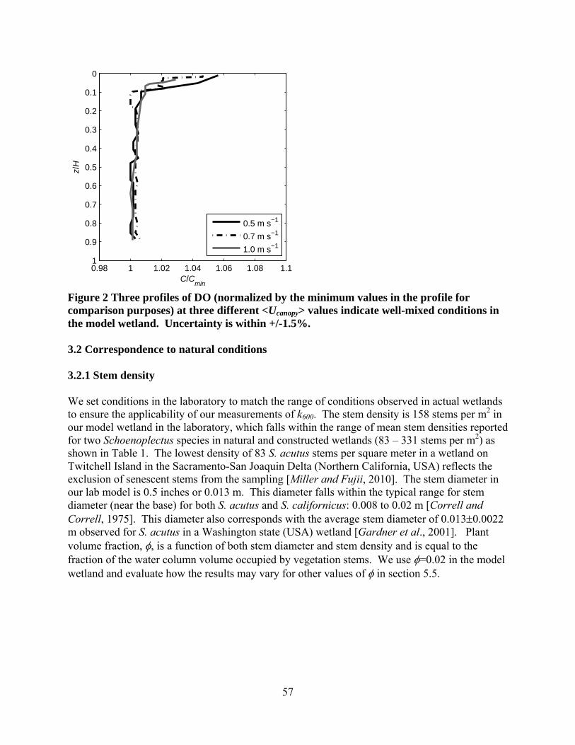
57

Figure 2 Three profiles of DO (normalized by the minimum values in the profile for comparison purposes) at three different <Ucanopy> values indicate well-mixed conditions in the model wetland. Uncertainty is within +/-1.5%. 3.2 Correspondence to natural conditions 3.2.1 Stem density We set conditions in the laboratory to match the range of conditions observed in actual wetlands to ensure the applicability of our measurements of k600. The stem density is 158 stems per m2 in our model wetland in the laboratory, which falls within the range of mean stem densities reported for two Schoenoplectus species in natural and constructed wetlands (83 – 331 stems per m2) as shown in Table 1. The lowest density of 83 S. acutus stems per square meter in a wetland on Twitchell Island in the Sacramento-San Joaquin Delta (Northern California, USA) reflects the exclusion of senescent stems from the sampling [Miller and Fujii, 2010]. The stem diameter in our lab model is 0.5 inches or 0.013 m. This diameter falls within the typical range for stem diameter (near the base) for both S. acutus and S. californicus: 0.008 to 0.02 m [Correll and Correll, 1975]. This diameter also corresponds with the average stem diameter of 0.0130.0022 m observed for S. acutus in a Washington state (USA) wetland [Gardner et al., 2001]. Plant volume fraction, , is a function of both stem diameter and stem density and is equal to the fraction of the water column volume occupied by vegetation stems. We use =0.02 in the model wetland and evaluate how the results may vary for other values of in section 5.5.

0.98 1 1.02 1.04 1.06 1.08 1.1

0

0.1

0.2

0.3

0.4

0.5

0.6

0.7

0.8

0.9

1

C/Cmin

z/H

0.5 m s−1

0.7 m s−1

1.0 m s−1

58

Table 1 Stem densities for Schoenoplectus acutus and Schoenoplectus californicus reported in the literature Mean stem density (stems m-2)

(assuming 0.5-inch stem diameter)

Species Sample site Location Sample date

Reference

83 0.011 S. acutus 6-ha restored wetland

Twitchell Island, CA, USA

1998-2006

Miller and Fujii, 2010

138 0.018 S. acutus and S. californicus

10-ha constructed treatment wetland

San Jacinto, CA, USA

Sep 1996

Sartoris et al., 2000

231 0.029 “ “ “ May 1997

“

192 0.024 S. acutus 20-ha wetland

Moses Lake, WA, USA

Aug 1994

Gardner et al., 2001

331 0.042 “ “ “ Aug 1995

“

3.2.2 Wind conditions Wind speed can vary greatly with vertical location in vegetation canopies. To maximize the applicability of our study, we use the most reproducible in-canopy velocity: the velocity in the shear-free region. In this region, <u’w’>0, and velocity is constant with z [Massman, 1987; Ghisalberti and Nepf, 2004]. This region is sometimes called the “wake” region, and we denote the velocity in this region <Ucanopy>. Predicting <Ucanopy> from more commonly measured wind parameters is non-trivial, though in crop canopies it has been found to scale with the shear velocity when the atmospheric boundary layer is neutral or unstable [Jacobs et al., 1995]. To our knowledge no measurements of in-canopy wind speed have been made in natural wetland canopies so we conducted field studies to determine the relevant range of <Ucanopy> in wetlands. We measured the horizontal wind speed profile within the 2.5-m tall emergent vegetation canopy of a restored wetland on Twitchell Island in the Sacramento-San Joaquin Delta (Northern Calif., USA). Typha spp. (cattail) and S. acutus are the dominant emergent vegetation species there [Miller and Fujii, 2010]. We measured wind speeds with a sonic anemometer, profiling heights from 0.25 m to 2 m above the water surface for a minimum of 10 minutes at each height. Because wind speed measurements at different heights were made sequentially over several hours, we normalized the data for the wind speed 2 m above the surface U2 from a nearby California Irrigation Management Information System (CIMIS) weather station (http://wwwcimis.water.ca.gov/). We collected one profile on a day when mean wind speed at the nearby weather station was 4.1 m s-1, close to the annual average, and a second on a calm day, both in October 2011. The wind speed profiles are shown in Figure 3, and indicate a nearly shear-free layer in the canopy near the water surface. In this shear-free layer <Ucanopy>0.1 m s-1 on the day with calm

59

wind and <Ucanopy>0.3 m s-1 on the day with average above-canopy wind. In-canopy winds gusted up to 1.7 m s-1 on the windier day. Laboratory wind tunnel air-flows were also uniform over z, as shown in three laboratory-measured velocity profiles in Figure 3. The range of wind speeds we use in the laboratory covers the range of wind speeds found in the field, in terms of both 10-minute average wind speeds and gusts. To get a sense of the distribution of canopy wind speeds at the restored wetlands on Twitchell Island, we compare (1) our measurements of <Ucanopy> at the restored wetlands on 19 October 2011, (2) <U2> at the Twitchell Island CIMIS weather station during the measurements, (3) the long-term (15-year) wind speed record at the CIMIS weather station. These data suggest that <Ucanopy> will be 0.3 m s-1 or less more than 50% of the time and that on occasion <Ucanopy> may be much higher.

Figure 3 Profiles of average horizontal wind speed, U, versus height above the water surface in both the model wetland in the laboratory and the Twitchell Island wetlands. Profiles confirm the presence of a constant-velocity region near the water surface. For reference we plot wind speed above the Twitchell Island wetland canopy (at 3 m above the water surface) obtained by scaling from a nearby weather station’s measurement of U2 (assuming constant shear velocity and applying typical relationships for the zero-plane displacement and roughness length). 3.2.3 Heat fluxes In a variety of wetlands, q was observed to range between –200 W m-2 and +300 W m-2. Specifically, in a 0.5-m deep Nebraska (USA) marsh with 3-m tall emergent vegetation (Phragmites australis) on a typical summer day, 2-hour average heat flux peaked at (170 – 200 W m-2) about the same time as the peak in incoming radiation [Burba et al., 1999b]. At night these heat fluxes were typically between –20 and – 70 W m-2 (averaging –45 W m-2) and were as

0 0.5 1 1.5 2 2.5 30

0.5

1

1.5

2

2.5

3

U (m s−1)

Hei

ght a

bove

wat

er s

urfa

ce (

m)

Wetland profile 1 (field)Wetland profile 2 (field)Wetland canopy height (field)Model wetland profile 1 (lab)Model wetland profile 2 (lab)Model wetland profile 3 (lab)Range <U

canopy> tested in lab

60

strong as -140 W m-2 over the measurement period of June to October [Burba et al., 1999a, 1999b]. A 6-day study of an Indiana (USA) marsh with 1-m tall emergent vegetation in June showed peak half hourly average heat loss rates of about -100 W m-2 each night. The maximum rate of heat flux into the water column was roughly 300 W m-2 each day [Souch et al., 1996]. To understand the distribution of surface heat fluxes, we calculate surface heat fluxes for the restored wetlands at Twitchell Island in the Sacramento-San Joaquin Delta using surface water temperature data provided by the USGS (Bryan Downing, personal communication, 2 Nov 2010). Our calculations of heat efflux (including radiant, sensible and latent heat) assume (1) negligible heat flux to the soil, (2) vertically homogenous temperature through the bulk of the water column and (3) negligible horizontal heat transport. Analysis of summer 2010 water temperature data from four temperature monitoring sites in the wetlands indicates median nighttime (8 AM – 8PM) heat loss of -40 W m-2 and a median daytime heat gain of +40 W m-2. For all four monitoring locations, the 2-hour average heat flux never exceeded 300 W m-2 or dropped below -200 W m-2 (Figure 4). The combined average diurnal pattern of heat flux for June-July 2010 followed the average diurnal pattern of total solar radiation at the nearby CIMIS weather station for the same period (Figure 5).

Figure 4 Histograms of 2-hour average heat flux across the air-water interface at the Twitchell Island wetlands for June-July 2010. Subplots (a) and (b) show histograms during the night (8pm – 8am) and day, respectively. The direction of nighttime heat flux is out of the wetland (q < 0) 86% of the time while the direction of daytime heat flux is into the water column (q > 0) 82% of the time.

−200 −100 0 100 200 3000

5

10

15

20

q W m−2

% o

f tim

e

a

−200 −100 0 100 200 3000

5

10

15

20

q W m−2

% o

f tim

e

b

61

Figure 5 The average diurnal pattern for June-July 2010 of heat flux (q) at the Twitchell Island wetlands and total solar radiation (R) at the nearby CIMIS weather station 4. Results Laboratory results for k are shown in Figure 6 as a function of <Ucanopy> and q. Circles represent those measurements preceded by surface skimming to obtain a repeatable level of surface cleanliness. For the skimmed cases and <Ucanopy> greater than 0.9 m s-1, the results are closely clustered at approximately 3 cm hr-1. In one notable exception with strong negative heat flux (q<-200 W m-2), k600 was 5.1 cm hr-1, indicating the importance of thermal convection. For <Ucanopy> greater than 0.9 m s-1, omitting the skimming step prior to measurement resulted in greater spread in the k600 data as well as lower median value of k600 (2.3 versus 3.0 cm hr-1). For <Ucanopy> less than 0.7 m s-1, there is no discernible trend between <Ucanopy> and k600. Instead k600 appears to increase as heat flux becomes negative and drops further below zero. The lowest value of k600 occurs when heat flux is positive (q=46 W m-2). To investigate the role heat flux played on gas transfer in the model wetland in the laboratory, we identify an analytical relationship between q and k.

00 02 04 06 08 10 12 14 16 18 20 22 00−80

−60

−40

−20

0

20

40

60

80

100

Hour

W m

−2

R/10q

62

Figure 6 Gas transfer velocity k600 versus mean in-canopy wind speed in the model wetland in the laboratory <Ucanopy>. Marker shade indicates the interfacial heat flux q in W m-2 during the measurement. Circles signify that the water surface was skimmed prior to measurement of k. Squares signify no skimming. Vertical error bars represent 95% confidence intervals. 5. Analysis and Discussion 5.1 Analytical model for k versus q Sufficient conditions for convective mixing occur when the water is losing heat to the air (q < 0). The heat transfer velocity kh is analogous to the gas transfer velocity. And as in equation 2, using the Prandtl number Pr (for heat) and a Schmidt number of 600 (for mass), we can scale the heat transfer velocity kh to the mass transfer velocity k600.

n

h Prkk

600600 (7)

We employ the standard definition for heat transfer velocity, in analogy to equation 1:

hp

qk

c T

(8)

0 0.2 0.4 0.6 0.8 1 1.20

1

2

3

4

5

6

<Ucanopy

> (m s−1)

k 600 (

cm h

r−1 )

q > 0−100 < q <= 0−200 < q <= −100q < −200

63

where T is the difference between the temperature at the water surface and the bulk water temperature. Using this definition, we nondimensionalize q by the thermal conductivity, a lengthscale L (which drops out later in our analysis), and T to obtain the Nusselt number:

α

LkNu h (9)

Nu can be considered the ratio of the total heat transfer to the heat transfer by molecular diffusion alone ( is the molecular diffusivity of heat). When the additional heat transfer beyond molecular diffusion is due to stirring by thermal convective motions, we can find the Nusselt number using semi-empirical relationships. These relationships are parameterized in terms of the Rayleigh number (RaT), which compares the convective transport of heat to opposing viscous and diffusive effects. For high Raleigh number flow (RaT > 8 x 106) below a cold horizontal boundary:

1/30.14 TNu Ra ±7% (10)

[Martynenko and Khramtsov, 2005]. While RaT is defined in terms of a temperature difference, there is also a flux Rayleigh number, Raq, that is a function of heat flux q, instead:

4

2qp

qgBLRa

c

for q<0 (11)

where B is the thermal expansion coefficient, g is gravitational acceleration, is the thermal diffusivity and is the kinematic viscosity. The two Rayleigh numbers are related through the Nusselt number [Bejan, 1995].

Nu

RaRa q

T (12)

Combining equations 9, 10, 11, 12 we obtain an expression for the heat transfer velocity. Applying the scaling relationship in equation 7 yields an expression for the gas transfer velocity.

n

p Prc

qgBk

60014.0

4/12

4/3600

for 0q and 6108TRa (13)

This analysis indicates that the gas transfer velocity for thermal convection is proportional to the heat loss, -q, to the one-fourth power. This relationship holds for negative flux values (heat loss) only, and for a minimum level of thermal or buoyant convection (RaT > 8 x 106). Using the wetland depth as the length scale, L, and assuming water temperatures of 10 C or higher, we find that the Rayleigh number exceeds this minimum threshold in wetlands of depth 0.4 m as long as q –2 W m-2. As seen in section 3.3, this condition is almost always satisfied. In contrast, for wetland water columns less than 0.10 m in depth, the Rayleigh number threshold for

64

equations 10 and 13 is not met for typical heat loss rates. For these shallow wetlands where RaT < 8 x 106, the Nusselt number is proportional to RaT to the one-fourth power rather than the one-third power [Martynenko and Khramtsov, 2005], resulting in a different relationship between k600 and q. The uncertainty in equation 13 is dominated by the reported 7% uncertainty in equation 10 and a 10% error in equation 2 when n is known to within 0.02 [Jähne and Haußecker, 1998]. Both experiments and theory indicate that the exponent in the Schmidt scaling relationship is 2/3 for no-slip interfaces and 1/2 for perfectly clean, free slip interfaces [Jähne et al., 1987]. Key assumptions in our treatment of convective interfacial flux are that (1) the formula for convection below a flat plate applies to convection below a free surface and (2) vegetation stems rising through the water column have negligible effect on thermal convection. Previous research suggests that these assumptions are valid. Assumption (1) is supported by experimental evidence indicating that the exponent in the Nu-Ra relationship was unchanged from the classic flat plate scenario when considering thermal convection below a cool skin at a free surface [Katsaros et al., 1977]. To evaluate assumption (2), we first approximate interstitial spaces as vertically oriented cylinders. Experimental measurements of convection inside cylinders of varying aspect ratio reveal that aspect ratio does not substantially alter the Nu-Ra relationship [Nikolaenko et al., 2005; Sun et al., 2005]. A second argument draws on the results of numerical simulations that have shown that the characteristic horizontal length scale of convection cells generated by a cool skin at a free surface is on the order of 0.05 m for a heat flux of -100 W m-2 [Leighton et al., 2003]. The characteristic inter-stem spacing in our lab experiment is 0.08 m, thus the presence of stems should not interfere with convective motions. It is not until vegetation densities of > 6% that the inter-stem spacing is similar to the size of convection cells. Equation 13 for k600 versus q is similar to that derived by Soloviev et al. [2007] using a different approach, namely the calculation of turbulent kinetic energy dissipation from buoyancy flux and calculation of k from dissipation. Soloviev et al. [2007] use a value of 0.253/4 for the coefficient rather than 0.143/4, which results in k600 values approximately 50% higher than those derived from equation 13 for n=1/2. 5.2 Coupled and independent effects of wind shear and thermal convection We calculate using equation 13 the value of k600 that would be expected if all observed interfacial gas flux in the model wetland in the laboratory was caused by thermal convection alone. The amount by which observed k600 values exceed this predication is an indication of how much wind stirring enhances k600. This difference can be seen in Figure 7 by comparing observations (points) to model predictions (lines). The two model lines correspond to the end-member cases of surface cleanliness: n=1/2 and n=2/3.

65

Figure 7 k600 measurements in the laboratory compared with k600 values expected as a result of thermal convection alone (determined from equation 13 and the heat flux q). Laboratory measurements are grouped into three wind speed classes, indicated by marker shade. Circles represent individual measurements of k made after skimming the surface to remove surfactants. Error bars represent 95% confidence intervals for these measurements. Squares indicate the mean of a number of measurements of k made without first skimming the surface. Error bars show the entire range of these measurements. A model for k600 as a function of heat flux is plotted for a free slip or perfectly clean surface (solid line) and a no-slip or contaminated surface (dashed line) with model uncertainty estimates (dotted lines). We first consider gas transfer velocities measured at the highest canopy wind speed (0.9 - 1.1 m s-1), shown in charcoal gray in Figure 7. In the case of three measured k600 values to the right of the origin, where we know convection is not contributing to gas transfer because the water column is gaining heat (q>0), there is a consistent value of k600 of approximately 3 cm hr-1. We take 3 cm hr-1 as the independent value of interfacial transport by wind at <Ucanopy>1 m s-1. Except for one data point, observed k600 values at <Ucanopy> greater than 0.9 m s-1 are also approximately 3 cm hr-1 to left of the origin where heat flux is negative. These k600 values are each less than the sum of k600 predicted from heat flux and the independent value of k600 for wind-driven stirring alone. Wind shear apparently overwhelms the effects of increasing surface heat loss when <Ucanopy> is greater than 0.9 m s-1 and q>-200 W m-2. When q=-310 W m-2, the observed k600 is equal to the value predicted from the heat flux (2 cm hr-1) plus the independent value of k600 for wind alone (3 cm hr-1).

−400 −300 −200 −100 0 100 2000

1

2

3

4

5

6

q (W m−2)

k 600 (

cm h

r−1 )

0.9 to 1.1 m s−1

0.7 to 0.9 m s−1

< 0.7 m s−1

66

All observed k600 values measured with <Ucanopy> less than 0.7 m s-1 and q<0, shown as white markers in Figure 7, fall between the upper and lower uncertainty bounds for k600 predictions due to thermal convection alone This suggests that when wind speeds are low and q is less than zero, q alone determines k600. A similar regime is observed in the open ocean where a threshold of U10 5 m s-1 has been identified as the cutoff between convective-dominated gas transfer and wind-dominated gas transfer [Soloviev and Schlüssel, 1994; Soloviev and Klinger, 2010]. When wind speeds are low and q is greater than zero, we find that k600 is very small but nonzero. Specifically, at a wind speed of 0.3 m s-1 and q = 46 W m-2 we measured the lowest gas transfer velocity in this study. Specifically, we measured k600 =0.11 cm hr-1, which is substantially lower than the other measurements made at low wind speeds. The drop in k600 as heat flux changes direction is what would be expected for gas transfer that is dominated by thermal convection. From the above analyses, we conclude that wind-driven mixing alone was responsible for the gas transfer velocities of 2.6-3.3 cm hr-1 measured at <Ucanopy> of 0.9-1.1 m s-1 as well as the gas transfer velocity of 0.11 cm hr-1 measured at a <Ucanopy> of 0.3 m s-1. These conclusions` suggest that k600 due to wind alone can be modeled as a non-linear function passing through the origin (for surfactant-free surfaces): k600=A<Ucanopy>

2 where A3 cm hr-1 m-2 s2. We choose to use a quadratic function in analogy with the results of Wanninkhof [1992] for much higher wind speeds in the ocean. Other functional forms are possible and the fit would benefit from more data, but this approximate result is sufficient for the remainder of our analysis. 5.3 Implications for wetland gas fluxes Field measurements suggest that is very rare for <Ucanopy> to exceed 0.7 m s-1, but that nighttime q averages -40 W m-2 in wetlands. Thus thermal convection will typically dominate wind shear in setting k600 in wetlands with emergent vegetation. In contrast, the wind is the dominant factor determining k in oceans. Lakes fall in the regime between wetlands and oceans, with both wind shear and surface heat loss driving gas transfer, and the relative importance of these two forcings set by lake area. For example, in a study of forty lakes, thermal convection was estimated to drive no more than 21% of the total gas transfer in large lakes, while in small lakes up to 79% of the total gas transfer was due to thermal convection [Read et al., 2012]. The increased importance of convection in small lakes is attributed to the increased topographic sheltering around these lakes [Read et al., 2012]. Because emergent vegetation in wetlands shelters the water surface even more effectively, it is logical that convection should dominate in wetlands with emergent vegetation. The dominance of thermal convection suggests that gas transfer velocity will exhibit a stronger diurnal variation in wetlands than in most lakes. This is because daytime values of k600 will drop nearly to zero during the day when q>0, and then increase significantly at night when surface cooling yields thermal convection. Laboratory measurements suggest that the daily variation in k600 will be roughly an order of magnitude, from k6000.1 cm hr-1 to k6001 cm hr-1. Equation 13 was derived in a way that should apply to natural wetlands, and its predictive capability was confirmed in our laboratory experiments. Thus we can apply this equation to predict k600 values and gas transfer in natural wetlands, assuming that no other forcing (wind, rain, current, waves, etc.) is significant. The strongest cooling heat flux typically observed in

67

wetlands is -200 W m-2, causing a maximum k600 between 1 and 2 cm hr-1 depending on value of the exponent n. For wetland air-water interfaces, n falls between 1/2 and 2/3. Biological activity provides a significant source of surfactant contamination, which increases n towards 2/3. While surfactants increase n towards 2/3, n can also be lowered towards 1/2 by dilational surface flows that disrupt the surfactant layer [Jähne et al., 1987]. In wind-driven currents, persistent dilational regions form adjacent to plant stems (as we will show in Section 5.5). If we assume conservatively that n=2/3, equation 13 predicts that the typical nighttime k600 value will be 0.6 cm hr-1, based on a typical nighttime q value of -45 W m-2 (as measured in Nebraska marsh [Burba et al., 1999a]). DO levels in emergent vegetation are often near zero [e.g. Rose and Crumpton, 1996] while the DO value in equilibrium with the atmosphere is approximately 10 g m-3 at 15 C. Assuming respiration keeps DO near zero in the bulk of the water column, the total nighttime flux due to hydrodynamic transport is thus 1 g m-2. As a point of comparison this flux is the same order of magnitude as most estimates of daily plant-mediated oxygen flux in wetlands compiled by Kadlec and Knight [1996]. Some wetland biogeochemical models do not include the hydrodynamic transport of dissolved methane and/or oxygen, assuming that the other gas transport pathways dominate [Walter and Heimann, 2000; Potter, 1997; Cao et al., 1996; Zhuang et al., 2002], but this sample calculation suggests otherwise, at least in the case of oxygen. On those rare occasions when strong winds cause shear-driven stirring of the water surface, our measurements suggest that k600 values will be roughly five times the typical nighttime value due to thermal convection alone. The factor of five is large, but not so large as to completely overwhelm the effects of daily average gas transfer. Thus it is not clear whether overall gas transfer in wetlands is dominated by rare or average events. Future work could answer this question by considering the joint probability distribution of wind, heat flux, and dissolved gas concentration. 5.4 Accounting for increased wind speed variance in real emergent plant canopies The influence of extreme winds on k600 in wetlands suggests that we should consider the role of gusts, even when the time-averaged wind speed is small. Natural wind forcing varies over a wide range of timescales, and interactions between the wind and plant canopy generate intermittent, large-scale eddies [Raupach et al., 1996]. As a result, the variance of wetland in-canopy velocity is much greater in the field than in our laboratory model. For example, in the lab the fluctuation

intensity, canopy

1/2

canopycanopy UUU 2 , is 0.11±0.01. At the wetlands on Twitchell

Island in the Sacramento-San Joaquin Delta, the fluctuation intensity is 0.57±0.05. This additional variance will affect k and can be expressed as an enhancement factor, as used for example by Wanninkhof et al. [2004] for wind in the ocean. We find the enhancement factor by

conducting a Monte Carlo analysis using the approximate relationship: 2600 3 canopyUk . When

Ucanopy has a stochastic distribution, then 2 2600 3 3canopy canopyUk U where is an

enhancement factor. We can evaluate by specifying a distribution of Ucanopy values as the Monte Carlo model input.

68

Figure 8 k600 enhancement factor as a function of Ucanopy fluctuation intensity The predicted enhancement factors are not sensitive to either <Ucanopy> or the kurtosis of the velocity distribution, both of which can vary significantly in environmental settings. The effect of velocity variance on is shown in Figure 8, from which it is evident that a fluctuation intensity of 0.11, as measured in the lab, is essentially equivalent to a fluctuation intensity of zero. For a fluctuation intensity of 0.57 as observed at the wetlands on Twitchell Island, the enhancement factor is 1.3; hence k600 values measured in the laboratory as a result of wind-induced stirring should be increased by 30% for these wetlands. This method inherently assumes that each temporary wind velocity affects the flow in the same way as a steady flow does. This may not be true, as acceleration and deceleration could have an additional effect on k. However, this assumption serves as a reasonable first approximation, given that many of the fluctuations observed in the field last long enough that they could be approximated as steady. Specifically, spectral analysis of field data collected within the shear-free region, at z=442 cm above the air-water interface, shows that 80% of the Ucanopy variance is due to motions lasting longer than 4 seconds. We use <Ucanopy> to predict wind-driven gas transfer because <Ucanopy> is directly related to the wind shear at the water surface, which influences gas exchange. However, <Ucanopy> is not readily available from meteorological data. Instead, it must be measured using anemometers installed in the emergent canopy. Such efforts may be cost-prohibitive, especially when the results at stake are a change in k600 of order 1 cm hr-1. In cases where <Ucanopy> must be known and cannot be measured, a relationship can likely be derived using U10, shear velocity, and the emergent canopy geometry. Alternatively, 1.5-order turbulence closure models have been found to successfully predict <Ucanopy> from profiles of leaf area index [Katul et al., 2004]. 5.5 Applicability of results to different plant volume fractions

⟨(U−⟨Ucanopy

⟩)2⟩1/2/⟨U⟩

β

β=1.01±0.01←

β=1.32±0.04

Lab

Fiel

d

0 0.2 0.4 0.6 0.8 11

1.1

1.2

1.3

1.4

1.5

1.6

1.7

1.8

1.9

2

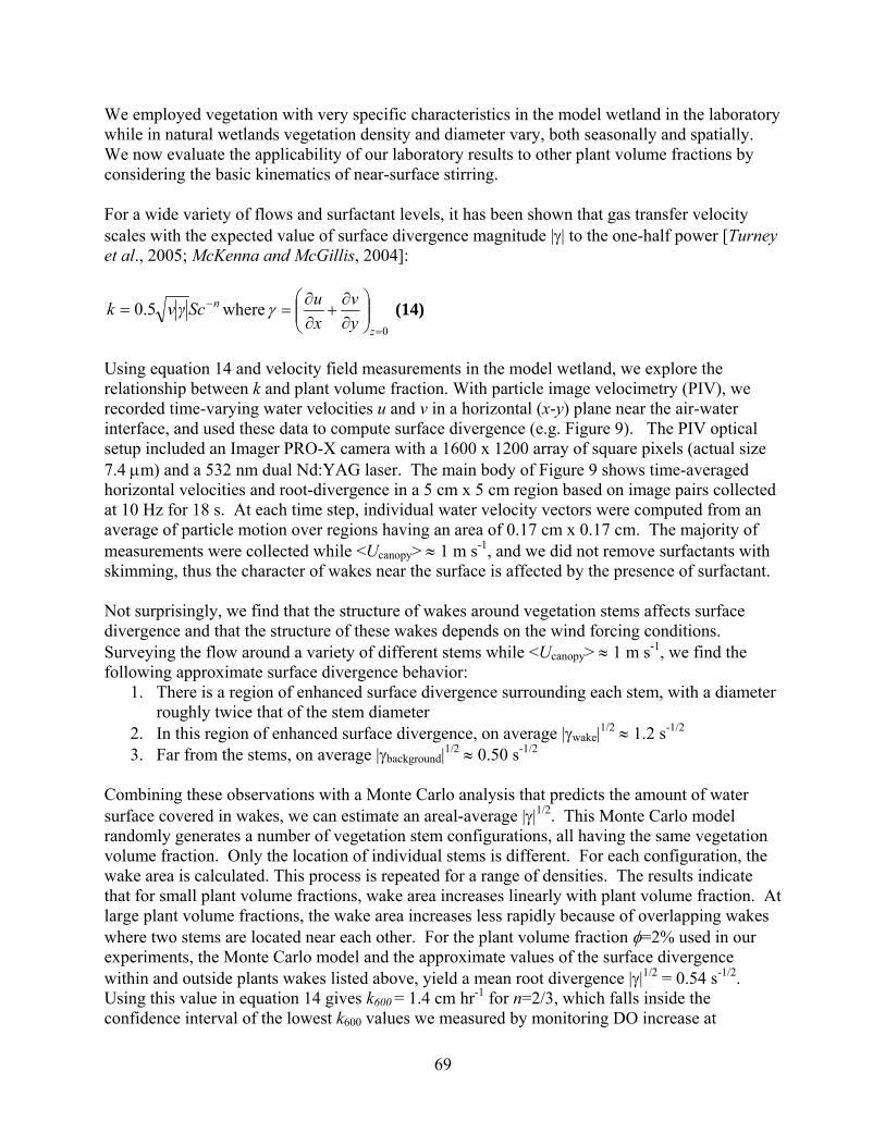
69

We employed vegetation with very specific characteristics in the model wetland in the laboratory while in natural wetlands vegetation density and diameter vary, both seasonally and spatially. We now evaluate the applicability of our laboratory results to other plant volume fractions by considering the basic kinematics of near-surface stirring. For a wide variety of flows and surfactant levels, it has been shown that gas transfer velocity scales with the expected value of surface divergence magnitude || to the one-half power [Turney et al., 2005; McKenna and McGillis, 2004]:

nScγνk 5.0 where0

z

y

v

x

u (14)

Using equation 14 and velocity field measurements in the model wetland, we explore the relationship between k and plant volume fraction. With particle image velocimetry (PIV), we recorded time-varying water velocities u and v in a horizontal (x-y) plane near the air-water interface, and used these data to compute surface divergence (e.g. Figure 9). The PIV optical setup included an Imager PRO-X camera with a 1600 x 1200 array of square pixels (actual size 7.4 m) and a 532 nm dual Nd:YAG laser. The main body of Figure 9 shows time-averaged horizontal velocities and root-divergence in a 5 cm x 5 cm region based on image pairs collected at 10 Hz for 18 s. At each time step, individual water velocity vectors were computed from an average of particle motion over regions having an area of 0.17 cm x 0.17 cm. The majority of measurements were collected while <Ucanopy> 1 m s-1, and we did not remove surfactants with skimming, thus the character of wakes near the surface is affected by the presence of surfactant. Not surprisingly, we find that the structure of wakes around vegetation stems affects surface divergence and that the structure of these wakes depends on the wind forcing conditions. Surveying the flow around a variety of different stems while <Ucanopy> 1 m s-1, we find the following approximate surface divergence behavior:

1. There is a region of enhanced surface divergence surrounding each stem, with a diameter roughly twice that of the stem diameter

2. In this region of enhanced surface divergence, on average |wake|1/2 1.2 s-1/2

3. Far from the stems, on average |background|1/2 0.50 s-1/2

Combining these observations with a Monte Carlo analysis that predicts the amount of water surface covered in wakes, we can estimate an areal-average ||1/2. This Monte Carlo model randomly generates a number of vegetation stem configurations, all having the same vegetation volume fraction. Only the location of individual stems is different. For each configuration, the wake area is calculated. This process is repeated for a range of densities. The results indicate that for small plant volume fractions, wake area increases linearly with plant volume fraction. At large plant volume fractions, the wake area increases less rapidly because of overlapping wakes where two stems are located near each other. For the plant volume fraction =2% used in our experiments, the Monte Carlo model and the approximate values of the surface divergence within and outside plants wakes listed above, yield a mean root divergence ||1/2 = 0.54 s-1/2. Using this value in equation 14 gives k600 = 1.4 cm hr-1 for n=2/3, which falls inside the confidence interval of the lowest k600 values we measured by monitoring DO increase at

<Ucanopy>of our menear the sdivergen

Figure 9correspo<Ucanopy>of high dthe regio Combininmodel fovaries wik varies aintercept volume fin S. acutvalues, wconvectiolargely in

> 1 m s-1. ethodology. stems. Unlikce above bac

9 Average floonding root > is approxidivergence oons marked

ng our approor wake-area ith plant volualmost linearat =0. For

fraction. Thitus marshes

wind plays a on is unlikelnsensitive to

The agreem For <Ucanop

ke the high wckground is

ow around divergence

imately 1 mof diameter “no data”,

oximate surffraction and

ume fractionrly with ovr n=2/3, the sis suggests th(0.01 – 0.04role in gas tr

ly to be affec at <Ucanop

ent betweenpy> 0.2 m swind speed cvisible near

stems near (backgroun

m s-1 in the m2d where da stem obst

face divergend the surfacen at this windver the commslope is 0.06hat k600 will

4), in cases wransfer subocted by plantpy >1 m s-1

70

n these indeps-1, the surfacase, only thstems (e.g.

the air-watnd) in the mmain figure d is the stem tructed cam

nce data for e divergence d speed. Formon range o6 cm hr-1 perbe essential

where <Ucano

ordinate to tht volume fracan be attrib

pendent measace divergenche slightest inFigure 9 ins

ter interfacemodel wetlan

and 0.2 m sm diameter wmera access.

<Ucanopy > model for kr the same <f plant volumr percentage lly the same opy >1 m s-1

hermal conveaction for lbuted to the s

surements sece is reducedncrease in su

set).

e (vectors) and in the labs-1 in the inswhen <Ucano

1 m s-1, the Mk, we can pre<Ucanopy> andme fractionspoint increaover the ran

1. (At lower ection and thess than 0.06small size of

erves as a chd, particularlurface

and the boratory. set. Note re

py>1 m s-1

Monte Carloedict how k d stem diames and has a laase in plant nge of obse

<Ucanopy> hermal 6.) That k isf the high

heck ly

egion 1. In

o

eter, arge

erved

s

71

divergence region around each stem. This suggests that the regions of enhanced stirring in plant wakes plays a minor role in gas transfer, at least in the presence of surfactants. We cannot rule out a greater role for wakes (and increased variability of k with ) when surfactants are absent or for larger diameter plants, which would produce larger wakes at the same wind speed. Because gas transfer is driven by surface divergence, the relevant vegetation density is that measured very near the water surface, and the vertical variation in the bulk water column need not be considered for predicting wind-driven interfacial flux. This is a useful simplification, as stem density can vary significantly with vertical location in the water column, either due to individual plant morphology or community morphology (e.g. the high density of “thatch” near the sediment-water interface). 5.5 Implications for wetland gas flux measurement and modeling The strong diurnal pattern in gas transfer velocity we predict for typical or calm meteorological conditions may have implications for wetland gas flux measurement. Chamber-based measurements of gas flux are often made during the day [e.g. Miller, 2011; Matthews et al., 2003], however, typical daytime conditions in wetlands yield the lowest gas transfer velocities (Table 2). This can cause a significant downward bias in measured fluxes when measurements are made only during the day. Quasi-continuous eddy covariance measurements are less likely to be affected by this bias. Our results provide an opportunity for users of floating chambers to estimate how much mass transfer they are missing by eliminating wind effects and altering heat exchange in general. Floating chambers may interfere with all forms of heat exchange between the water and atmosphere, and consequently thermal convection in the water column that leads to interfacial flux. At high canopy wind speeds, floating chambers could also reduce k600 by impeding the wind’s direct mechanical stirring of the water column. When considering these biases, it is important to note that the error due to reduced wind mixing and thermal convection in chambers could be outweighed by error due to motions generated by the floating chamber itself. Floating chambers have been found to artificially increase near-surface turbulence. For example, in lakes under calm conditions, chambers have been seen to increase k600 by between 50% and 1000% [Vauchon et al., 2010]. Process-based wetland carbon models are important for constraining greenhouse gas uptake and emissions by wetlands now and in a future of changing climate. Such models can help explain the observed spatial and temporal variability in methane emissions and carbon sequestration across different wetland types and climates [Kayranli et al., 2010], and differentiate methane production from methane consumption, which is estimated to be equal to 60% of terrestrial methane production globally [Riley et al., 2011]). By including dissolved gas fluxes across the air-water interface and parameterizing them with k600 rather than the molecular diffusivity, process-based carbon models will more accurately capture wetland dynamics. Hourly or half-hourly time step models [e.g. Riley et al., 2011] could implement the full diurnal pattern in k600. For models with daily time steps [e.g. Walter and Heimman, 2001] diurnal k variation due to alternating direction of heat flux should be accurately accounted for by appropriate averaging.

72

5.6 Comparison with gas transfer models and data from lakes In Figure 10, we plot our results along with data and models for k600 from the literature. The models were derived from measurements of k600 in lakes [MacIntyre et al., 2010; Cole and Caraco, 1998]; the points represent individual measurements made in a wetland pond free of emergent vegetation [Sebacher et al., 1983]. On the x-axis in the plot is the wind speed at a height of 0.4 m above the water surface, the height at which we measured wind speedin our measurements of k600 in the model wetland. MacIntyre et al. [2010] and Cole and Caraco [1998] report wind speed 10 m above the water surface while Sebacher et al. [1983] measured wind speeds 0.02 m above the water surface. We scaled these wind speeds to a height of 0.4 m above the water surface using a typical value for the roughness height over open water. The regression of MacIntyre et al. [2010] for q>0 and to a lesser extent the model of Cole and Caraco [1998] fit our laboratory data collected while <Ucanopy> exceeded 0.7 m s-1. The k600 value we measured for q=-310 W m-2 falls closer to the MacIntyre et al. [2010] regression for q<0 however. We surmise that compared to wetlands with emergent vegetation, surface heat fluxes in lakes are more often in the range of q<-300 W m-2, resulting in generally higher gas transfer velocities during periods of surface cooling. The wetland pond k600 measurement at a wind speed of 0.8 m s-1 by Sebacher et al. [1983] overlaps with our laboratory data; their measurement at zero wind speed does not. Empirical relationships derived in lakes and ponds may be sufficient for predicting gas transfer for high in-canopy wind speeds in wetlands with emergent vegetation if in-canopy wind speed is known. For in-canopy wind speeds less 0.7 m s-

1, there was no discernible, monotonic trend in the laboratory data with wind speed and it is preferable to model k600 as a function of heat loss.

Figure 10 Comparison of k600 values measured in our model wetland in the laboratory (stars) with data and models from the literature for lakes and ponds

0 0.2 0.4 0.6 0.8 1 1.20

1

2

3

4

5

6

7

8

<Uz=0.4 m

> (m s−1)

k 600 (

cm h

r−1 )

This work q<0This work q>=0MacIntyre et al. (2010) q<0MacIntyre et al. (2010) q>0Cole & Caraco (1998)Sebacher et al. (1983)

73

6. Conclusions We have used laboratory experiments to examine the relationship between interfacial gas flux and stirring by wind and thermal convection in wetlands with emergent vegetation. The experimental settings are based on field measurements in a Northern California marsh with an emergent plant canopy of Typha spp. and S. acutus, as well as data from similar wetlands in the literature. At in-canopy wind speeds equal to those measured in the field, gas transfer velocities in the model wetland were largely insensitive to in-canopy wind speed. Instead, thermal convection induced by heat loss at the water surface appeared to drive most hydrodynamic gas transfer. We saw evidence for this in the agreement between gas transfer velocities measured in the model wetland and gas transfer velocities predicted from a semi-empirical function of surface heat loss. For mean in-canopy wind speeds greater than those observed in the field, measured gas transfer velocities increased with increasing wind speed and exceeded those predicted to occur due to thermal convection alone. Based on these results, we infer a quadratic relationship between mean in-canopy wind speed and gas transfer velocity. Because of the high turbulent intensities observed in the wetland canopy in the field, an enhancement factor must be included in this relationship. Particle image velocimetry revealed regions of increased surface divergence, and hence increased air-water gas transfer, around emergent plant stems. With surfactants present, the combined area of these high-divergence regions is small, suggesting that variations in the density of plant stems do not directly affect wetland air-water gas transfer, and that the predominant effect of emergent stems on wind-driven gas transfer is the attenuation of the wind speed above the water surface. Indeed, k values measured in the model wetland at high in-canopy wind speed correspond with k values predicted by some empirical relationships for lakes once the wind speed in these relationships is scaled to a height below the canopy height. Regular nightly increases in k due to thermal convection are strong enough to make hydrodynamic gas transfer a significant component of the biogeochemical budget in wetlands with emergent vegetation. Air-water oxygen flux, assuming a reasonable value for the wetland water column dissolved oxygen and the surface heat loss, is likely of the same magnitude as plant-mediated oxygen flux. In addition, high in-canopy wind speeds, though rare, could cause spikes in air-water gas fluxes that contribute sizably to overall gas transfer. The predictive models for gas transfer velocity that we have identified can be used to approximate interfacial gas fluxes over a range of wind speeds and surface heat fluxes. Applications include partitioning eddy covariance measurements of net gas flux by transport pathway and more accurately representing gas transport in wetland biogeochemical models. References Augustin, L. N., J. L. Irish, and P. Lynett (2009), Laboratory and numerical studies of wave damping by emergent and near-emergent wetland vegetation, Coastal Engineering, 56(3), 332–340, doi:10.1016/j.coastaleng.2008.09.004.

74

Barber, T. R., R. A. Burke Jr., and W. M. Sackett (1988), Diffusive flux of methane from warm wetlands, Global Biogeochem. Cycles, 2(4), 411–425, doi: 10.1029/GB002i004p00411. Bejan, A. (1995), Convection Heat Transfer, John Wiley & Sons, Inc., New York, N.Y. Benson, B. B., and D. Krause Jr. (1984), The concentration and isotopic fractionation of oxygen dissolved in freshwater and seawater in equilibrium with the atmosphere, Limnol. and Oceanogr., 29(3), 620–632. Bock, E. J., T. Hara, N. M. Frew, and W. R. McGillis (1999), Relationship between air sea gas transfer and short wind waves, J. Geophys. Res., 104(C11), 25,821–25,831, doi: 10.1029/1999JC900200. Brix, H., B. K Sorrell, and B. Lorenzen (2001), Are Phragmites-dominated Wetlands a Net Source or Net Sink of Greenhouse Gases? Aquat. Bot. 69(2–4): 313–324. Burba, G. G., S. B. Verma, and J. Kim (1999a), A comparative study of surface energy fluxes of three communities (Phragmites australis, Scirpus acutus, and open water) in a prairie wetland ecosystem, Wetlands, 19(2), 451–457. Burba, G., S. Verma, and J. Kim (1999b), Surface energy fluxes of Phragmites australis in a prairie wetland, Agricultural and Forest Meteorology, 94(1), 31–51. Campbell Scientific (2012), CSAT3 Three Dimensional Anemometer Instructional Manual, Campbell Scientific Inc., Logan, Utah. Cao, M., M. Stewart and K. Gregson (1996), Global carbon exchange and methane emissions from natural wetlands: Applications of a process-based model, J. Geophys. Res. 101(9):14399-414, doi: 10.1029/96JD00219. Cionco, R. M. (1972), A wind-profile index for canopy flow, Boundary-Layer Meteorology, 3(2), 255–263. Cole, J.J. and N.F. Caraco (1998), Atmospheric exchange of carbon dioxide in a low-wind oligotrophic lake measured by the addition of SF6, Limnol. Oceanogr. 43(4), 647-56. Correll, D. S. and H. B. Correll (1975) Aquatic and wetland plants of Southwestern United States, Stanford University Press, Palo Alto, CA. Crusius, J., and R. Wanninkhof (2003), Gas transfer velocities measured at low wind speed over a lake, Limnol. Oceanogr., 48(3), 1010–1017. Denman, K.L., G. Brasseur, A. Chidthaisong, P. Ciais, P.M. Cox, et al. (2007): Couplings Between Changes in the Climate System and Biogeochemistry, in Climate Change 2007: The Physical Science Basis. Contribution of Working Group I to the Fourth Assessment

75

Report of the Intergovernmental Panel on Climate Change edited by Solomon, S. et al., Cambridge University Press, Cambridge, United Kingdom and New York, N.Y. Drexler, J. Z., F. E. Anderson and R. L. Snyder (2008), Evapotranspiration rates and crop coefficients for a restored marsh in the Sacramento-San Joaquin Delta, California, USA, Hydrol. Process., 22, 725-735. Eugster, W., G. Kling, T. Jonas, J. P. McFadden, A. Wüest, S. MacIntyre, and F. S. Chapin III (2003), CO2 exchange between air and water in an Arctic Alaskan and midlatitude Swiss lake: Importance of convective mixing, J. Geophys. Res., 108, D12, doi: 10.1029/2002JD002653. Finnigan, J. (2000), Turbulence in plant canopies, Annu. Rev. Fluid Mech., 32, 519-571. Gardner, S. C., C. E. Grue, W. W. Major, and L. L. Conquest (2001), Aquatic invertebrate communities associated with purple loosestrife (Lythrum salicaria), cattail (Typha latifolia), and bulrush (Scirpus acutus) in central Washington, USA, Wetlands, 21(4), 593–601. Ghaly, A. E. and R. Kok (1988), The effect of sodium sulfite and cobalt chloride on the oxygen transfer coefficient, Appl. Biochem. Biotechnol. 19(3): 259–270. Ghisalberti, M., and H.M. Nepf (2004), The limited growth of vegetated shear layers, Water Resour. Res, 40(7), W07502, doi: 10.1029/2003WR002776. Happell, J. D., J. P. Chanton, and W. J. Showers (1995), Methane transfer across the water-air interface in stagnant wooded swamps of Florida: Evaluation of mass-transfer coefficients and isotopic fractionation, Limnol. Oceanogr., 40(2), 290–298. Ho, D. T., L. F. Bliven, R. Wanninkhof, and P. Schlosser (1997), The effect of rain on air-water gas exchange, Tellus Ser. B, 49(2), 149–158. Jacobs, A. F. G.,H. van Boxel and M. El-Kilani (1995), Vertical and horiztonal distribution of wind speed and air temperature in a dense vegetation canopy, J. Hydrol., 166, 313-326. Jähne, B., and H. Haußecker (1998), Air-water gas exchange, Annu. Rev. Fluid Mech., 30(1), 443–468. Jähne, B., K. O. Münnich, R. B. A. Dutzi, W. Huber, and P. Libner (1987), On the parameters influencing air-water gas exchange, J. Geophys. Res., 92(C2), 1937–1949, doi: 10.1029/JC092iC02p01937. Kadlec, R. H., and R. L. Knight (1996), Treatment Wetlands, CRC Press, Boca Raton, FL. Kadlec, R.H. and S.D. Wallace (2009) Treatment Wetlands, CRC Press, Boca Raton, FL. Katsaros, K. B., W. T. Liu, J. A. Businger, and J. E. Tillman (1977), Heat transport and thermal structure in the interfacial boundary layer measured in an open tank of water in turbulent free convection, J83(2), 311–335.

76

Katul, G. G., L. Mahrt, D. Poggi, and C. Sanz (2004), One- and two-equation models for canopy turbulence, Bound.-Lay. Meteorol., 113(1), 81–109, doi:10.1023/B:BOUN.0000037333.48760.e5. Kayranli, B., M. Scholz, A. Mustafa, and Å. Hedmark (2010), Carbon Storage and Fluxes Within Freshwater Wetlands: a Critical Review, Wetlands 30(1), 111–124, doi: 10.1007/s13157-009-0003-4. Khakpour, H. R., L. Shen, and D. K. Yue (2011), Transport of passive scalar in turbulent shear flow under a clean or surfactant-contaminated free surface, J. Fluid Mech., 670(1), 527–557, doi: 10.1017/S002211201000546X. Knutson, P. L., R.A. Brochu, W.N. Seelig and M. Inskeep (1982), Wave damping in Spartina alterniflora marshes, Wetlands 2(1): 87–104. Leighton, R. I., G. B. Smith, and R. A. Handler (2003), Direct numerical simulations of free convection beneath an air–water interface at low Rayleigh numbers, Phys. Fluids, 15(10), 3181-3193. Li, T., Y. Huang, W. Zhang, and C. Song (2010), CH4MODwetland: A biogeophysical model for simulating methane emissions from natural wetlands, Ecol. Modell., 221(4), 666–680, doi: 10.1016/j.ecolmodel.2009.05.017. Lindberg, S. E., and H. Zhang (2000), Air/water exchange of mercury in the Everglades II: measuring and modeling evasion of mercury from surface waters in the Everglades Nutrient Removal Project, The Science of the Total Environment, 259(1-3), 135–143. MacIntyre, S., A. Jonsson, M. Jansson, J. Aberg, D. E. Turney, and S. D. Miller (2010), Buoyancy flux, turbulence, and the gas transfer coefficient in a stratified lake, Geophys. Res. Lett., 37, L24604, doi: 10.1029/2010GL044164. Maltais-Landry, G., R. Maranger, and J. Brisson (2009), Effect of artificial aeration and macrophyte species on nitrogen cycling and gas flux in constructed wetlands, Ecological Engineering, 35(2), 221–229, doi: 10.1016/j.ecoleng.2008.03.003. Martynenko, O. G., and P. P. Khramtsov (2005), Free-convective heat transfer: with many photographs of flows and heat exchange, Springer Verlag, Berlin. Massman, W. (1987), A Comparative Study of Some Mathematical Models of the Mean Wind Structure and Aerodynamic Drag of Plant Canopies, Bound.-Lay. Meteorol., 40(1), 179–197. McGillis, W. R., J.B. Edson, C.J. Zappa, J.D. Ware et al. (2004), Air-sea CO2 exchange in the equatorial Pacific, J. Geophys. Res, 109, C08S02, doi:10.1029/2003JC002256. McKenna, S. P. and W. R. McGillis (2004), The role of free-surface turbulence and

77

surfactants in air-water gas transfer, Int. J. Heat Mass Transfer 47(3), 539–553, doi: 10.1016/j.ijheatmasstransfer.2003.06.001. Miller, R. L. (2011), Carbon Gas Fluxes in Re-Established Wetlands on Organic Soils Differ Relative to Plant Community and Hydrology, Wetlands 31(6), 1055-1066, doi: 10.1007/s13157-011-0215-2. Miller, R. L. and R. Fujii (2010), Plant community, primary productivity, and environmental conditions following wetland re-establishment in the Sacramento-San Joaquin Delta, California, Wetlands Ecol. and Manage., 18(1): 1–16, doi: 10.007/s11273-009-9143-9. Nepf, H. M., J. A. Sullivan, and R. A. Zavistoski (1997), A model for diffusion within emergent vegetation, Limnol. Oceanogr., 42(8), 1735–1745. Nikolaenko, A., E. Brown, D. Funfschilling, and G. Ahlers (2005), Heat transport by turbulent Rayleigh-Bénard convection in cylindrical cells with aspect ratio one and less, J. Fluid Mech. 523, 251–260, doi: 10.1017/S0022112004002289. Potter, C.S. (1997), An ecosystem simulation model for methane production and emission from wetlands, Global Biogeochem. Cycles, 11(4), 495-506, doi: 10.1029/97GB02302. Raupach, M. R., J. J. Finnigan, and Y. Brunei (1996), Coherent eddies and turbulence in vegetation canopies: the mixing-layer analogy, Bound.-Lay. Meteorol., 78(3), 351–382. Riley, W. J., Z. M. Subin, D. M. Lawrence, S. C. Swenson, M. S. Torn, L. Meng, N. M. Mahowald, and P. Hess (2011), Barriers to predicting changes in global terrestrial methane fluxes: analyses using CLM4Me, a methane biogeochemistry model integrated in CESM, Biogeosciences 8, 1925–1953, doi: 10.5194/bg-8-1925-2011. Rudd, J. W. M. (1995), Sources of methyl mercury to freshwater ecosystems: a review, Water, Air, Soil Pollut., 80(1), 697–713. Read, J. S., D. P. Hamilton, A. R. Desai, K. C. Rose, S. MacIntyre et al. (2012), Lake-size dependency of wind shear and convection as controls on gas exchange, Geophys. Res. Lett., 39, L09405, doi: 10.1029/2012GL051886. Rose, C. and W. G. Crumpton (1996), Effects of emergent macrophytes on dissolved oxygen dynamics in a prairie pothole wetland, Wetlands, 16(4), 495-502. Sartoris J.J., J.S. Thullen, L.B. Barber & D.E. Salas (2000), Investigation of nitrogen transformations in a southern California constructed wastewater treatment wetland, Ecol. Eng., 14, 49-65. Schladow, S. G, M. Lee, B. E Hürzeler, and P. B Kelly (2002), Oxygen transfer across the air-water interface by natural convection in lakes, Limnol. Oceanogr., 47(5), 1394–1404.

78

Sebacher, D. I.,C. Harriss and K. B. Bartlett (1983), Methane flux from air-water interface: air velocity effects, Tellus, Ser. B 35(2), 103-109, doi: 10.1111/j.1600-0889.1983.tb00014.x. Soloviev, A.,Donelan, H. Graber, B. Haus and P. Schlüssel (2007), An approach to estimation of near-surface turbulence and CO2 transfer velocity from remote sensing data, J. Marine Syst. 66, 182-194, doi: 10.1016/j.jmarsys.2006.03.023 Soloviev, A. V. and B. Klinger (2001), Open ocean convection in Encyclopedia of Ocean Sciences, vol. 4, edited by J.H. Steele et al., pp. 2015-2022, Elsevier Ltd, Amsterdam. Soloviev, A. V., and P. Schlüssel (1994), Parametrization of the cool skin of the ocean and of the air-ocean gas transfer on the basis of modeling surface renewal, J. Phys. Oceanogr., 24(6), 1339–1346. Souch, C., C. P. Wolfe, and C. S. B. Grimmond (1996), Wetland evaporation and energy partitioning: Indiana dunes national lakeshore, J. Hydrol., 184(3-4), 189–208, doi: 10.1016/0022-1694(95)02989-3. Spieles, D. J., and W. J. Mitsch (2003), A model of macroinvertebrate trophic structure and oxygen demand in freshwater wetlands, Ecol. Modell., 161(3), 183–194, doi: 10.1016/S0304-3800(02)00342-3. Sun, C., L. Y. Ren, H. Song, and K. Q. Xia (2005), Heat transport by turbulent Rayleigh-Bénard convection in 1 m diameter cylindrical cells of widely varying aspect ratio, J. Fluid Mech., 542, 165–174, doi: 10.1017/S0022112005006610. Tian, H., X. Xu, M. Liu, W. Ren, C. Zhang, G. Chen, and C. Lu (2010), Spatial and temporal patterns of CH4 and N2O fluxes in terrestrial ecosystems of North America during 1979–2008: application of a global biogeochemistry model, Biogeosciences, 7(9), 2673–2694, doi: 10.5194/bg-7-2673-2010. Turney, D.E., W. C Smith, and S. Banerjee (2005), A measure of near-surface fluid motions that predicts air-water gas transfer in a wide range of conditions, Geophys. Res. Lett., 32(4), doi: 10.1029/2004GL021671. Vachon, D., Y. T. Prairie, and J. J. Cole (2010), The relationship between near-surface turbulence and gas transfer velocity in freshwater systems and its implications for floating chamber measurements of gas exchange, Limnol. Oceanogr., 55(4), 1723, doi: 10.4319/lo.2010.55.4.1723. Variano, E. A., D. T. Ho, V. C. Engel, P. J. Schmieder, M. C. Reid et al. (2009), Flow and mixing dynamics in a patterned wetland: Kilometer-scale tracer releases in the Everglades, Water Resour. Res, 45, W08422, doi: 10.1029/2008/WR007216. Walter, B. P. and M. Heimann (2000), A process-based, climate sensitive model to derive

79

methane emissions from natural wetlands, Global Biogeochem. Cycles, 14(3), 745–65, doi: 10.1029/1999GB001204. Wanninkhof, R. (1992), Relationship between wind speed and gas exchange, J. Geophys. Res., 97, 7373–7382, doi: 10.1029/92JC00188. Wanninkhof, R., K. F. Sullivan, and Z. Top (2004), Air-sea gas transfer in the Southern Ocean, J. of Geophys. Res., 109(C8), C08S19, doi: 10.1029/2003JC001767. Whiting, G. J., and J. P. Chanton (2001), Greenhouse carbon balance of wetlands: methane emission versus carbon sequestration, Tellus Ser. B, 53(5), 521–528, doi: 10.1034/j.1600-0889.2001.530501.x. Zappa, C. J., W. R. McGillis, P. A. Raymond, J. B. Edson, E. J. Hintsa, H. J. Zemmelink, J. W. H. Dacey, and D. T. Ho (2007), Environmental turbulent mixing controls on air-water gas exchange in marine and aquatic systems, Geophys. Res. Lett., 34(10), L10601, doi: 10.1029/2006GL028790. Zhang, H. H., L. Poissant, X. Xu, M. Pilote, C. Beauvais, M. Amyot, E. Garcia and J. Laroulandie (2006), Air-water gas exchange of mercury in the Bay of Saint Franҫois wetlands: Observations and model parameterization, J. Geophys. Res. 111, D17307, doi:10.1029/2005JD006930. Zhuang, Q., J. M. Melillo, D. W. Kicklighter, R. G. Prinn, A. D. McGuire, P. A. Steudler, B. S. Felzer, and S. Hu (2004), Methane fluxes between terrestrial ecosystems and the atmosphere at northern high latitudes during the past century: A retrospective analysis with a process-based biogeochemistry model, Global Biogeochem. Cycles, 18: GB3010, doi:10.1029/2004GB002239. Zhang, Y., C. Li, C.C. Trettin, H. Li & G. Sun (2002), An integrated model of soil, hydrology, and vegetation for carbon dynamics in wetland ecosystems, Global Biogeochem. Cycles 16(4): 1061-77 doi: 10.1029/2001GB001838.

80

Chapter 5 Overlooked hydrodynamic transport responsible for a significant portion of a marsh’s methane emissions 1. Introduction Methane levels in the atmosphere have tripled since pre-industrial times (Houghton et al., 2001), but an unexpected slowing in the rate of methane increase has occurred over the last few decades. It has been attributed to decreased emissions from rice paddies and northern wetlands (Kai et al., 2011) and alternatively to a decline in methane emissions from fossil fuel production (Aydin et al., 2011). Regardless, these fluctuations remain an enigma (Heimann, 2011). Wetlands are known to be single largest source of methane (Denman et al., 2007) and the primary driver of inter-annual variability in methane emissions (Bousquet et al., 2006). Improved bottom-up modeling of wetland methane emissions could help explain recent methane fluctuations as well as predict future methane levels. Bottom-up models predict methane production from inundation, net primary productivity and temperature and in many cases also account for methane transport to the atmosphere. Methane transport is important because of potentially large methane consumption en route to the atmosphere (e.g. King, 1990). One stumbling block to increased accuracy in bottom-up methane models is insufficient data on the relative contributions of the different methane transport processes in wetlands (Bridgham et al., 2013). There is evidence that wetlands with surface water emit more methane than wetlands where the water table remains at or below the ground surface (e.g. Sebacher et al., 1986; Moore and Knowles, 1989; Morrissey and Livingston, 1992). Nonetheless, dissolved methane transport in wetland surface water has received little attention. Methane transport to the atmosphere has been thought to occur mostly via ebullition (bubbling) or through the gas filled tissue (aerenchyma) of emergent vegetation (e.g. Van der Nat et al., 1998; Whiting and Chanton, 1992). Molecular diffusion of dissolved methane, often listed as the third gas transport mechanism (Whiting and Chanton, 1992; Sorrel and Boon, 1994; Van der Nat et al., 1998; Walter and Heimann, 2000; Gedney et al., 2004; Riley et al., 2011; Sharifi et al., 2013), is likely negligible because of its very slow pace in water. Hydrodynamic dissolved methane transport may not be negligible. Transport through the surface water and across the air-water interface due to the larger scale motions of the water depends on environmental factors. While wind is the most widely known driving force of air-water gas transfer, in sheltered small lakes, thermal convection has been shown to play a larger role (Read et al., 2012). Nightly pulses of methane coincident with thermally driven stirring of the water column have recently been observed in wetlands (Godwin et al., 2013). Still data to quantify hydrodynamic transport, including thermal convective transport, in wetlands with emergent vegetation have been lacking. The laboratory investigation of hydrodynamic dissolved gas transport in wetland surface water in Chapter 4 addressed this gap. The investigation yielded a model for the gas transfer velocity as a function of heat loss from the wetland water surface and additional data on the relationship between wind speed and gas transfer in wetlands. Here, using

81

those results, we model hydrodynamic methane transport, including thermal convective transport, at a temperate freshwater marsh. Thermal convection related to typical nighttime cooling in wetlands was associated with significant methane emissions in a natural wetland (Godwin et al., 2013) and substantial air-water gas exchange in a model wetland in the laboratory. Hence, we hypothesize that the hydrodynamic transport of methane, and particularly that due to thermal convection, represents a sizable portion of net methane emissions at our marsh study site. To test this hypothesis, we compare transport across the water column’s air-water interface modeled using the gas transfer velocity to total methane emissions measured via eddy covariance. The modeled and measured data span nearly a year, which allow us to draw robust conclusions about the role of hydrodynamic transport. The eddy covariance technique and our approach to obtaining air-water methane fluxes are non-intrusive and provide methane fluxes both during daylight hours and at night. Consequently our results may help resolve some of the continuing uncertainty about methane transport processes in wetlands. 2. Site description The marsh is located on Twitchell Island in the Sacramento-San Joaquin Delta region of Northern California, USA (latitude: 38 6’ N; longitude: 121 39’ W), approximately 100 km inland from the Pacific Ocean. Late-nineteenth and early-twentieth century draining of marshes in the region led to oxidation of the peat soil, and many areas, including the study site, have subsided meters below sea level (Rojstaczer and Deverel, 1995). The marsh was constructed by the California Department of Water Resources (CA DWR) and the United States Geological Survey (USGS) in 1997 as part of a pilot program to re-establish marshland to the Sacramento-San Joaquin Delta region for subsidence reversal. Small berms were built to isolate a 3-ha parcel and Schoenoplectus acutus (tule) shoots were planted across approximately 3% of the area. Typha spp. (cattail) colonized significant areas via wind-blown propagules (Miller et al., 2008) and a 2-4 m tall canopy of Typha spp. and S. acutus now covers 95% of the marsh (Miller and Fujii, 2010). The marsh’s water source is freshwater siphoned from the nearby San Joaquin River and conveyed via pipeline to inlets located on the southern edges of the marsh. Flow rates through the wetland are small, averaging 0.01 m3 s-1 and water velocities have been measured to be on the order of the a tenth of a millimeter per second (unpublished data). The average residence time is on the order of 3 days. An average water depth of 0.25 m is maintained by controlling the height of an outflow located on the northern edge of the marsh. Between summer 2012 and summer 2013, inflow into the wetlands occasionally stopped causing the wetlands to drain temporarily, most notably during October 2012. High levels of carbon uptake as well as substantial methane emissions were observed at the marsh between 1997 and 2003 using chambers (Miller, 2011) and the CA DWR is currently re-establishing additional marshes on nearby parcels.

3. Methods We measured total methane emissions at the marsh study site using the eddy covariance technique and compared total methane fluxes to modeled hydrodynamic transport of methane through the surface water for a nearly year-long study period (19 July 2012 – 27 June 2013).

82

3.1 Eddy covariance measurements of total methane emissions Net methane emissions were measured using the eddy covariance technique, in which high-frequency measurements of wind velocity and gas concentration are used to determine gas flux between the landscape and the atmosphere (Baldocchi et al., 1988). Scaffolding was erected in the spring of 2012 on the eastern edge of the re-established wetland and equipped with an open-path CO2/H2O infrared gas analyzer (LI-7500) and an open path methane analyzer (LI-7700) both manufactured by LI-COR Biogeosciences, Lincoln, NE, USA. The LI-7700 has a resolution of 5 ppb at 10 Hz (Licor) and is calibrated every 6 months. The LI-7500’s resolution is 0.11 ppm for CO2 and 0.0047 ppt for water vapor. It is calibrated every two to three months. A sonic anemometer (Wind Master 1590, Gill Instruments, Lymington, United Kingdom) is located within 0.3 m lateral distance of the infrared gas analyzers. A 4-component radiometer (NR01, Campbell Scientific, Locan, UT, USA), an aspirated and shielded temperature and humidity probe (HMP60, Vaisala, Helsinki, Finland) and a pressure transducer (PTB100, Vaisala, Helsinki, Finland) are also fixed to the scaffolding. The anemometer and gas analyzers stand approximately 4.7 m above the ground surface and approximately a meter above the top of the vegetation canopy during the growing season when the canopy reaches its peak height between 3 and 4 m. Gas fluxes are obtained half-hourly from the average of the co-variance of fluctuations in vertical wind velocity and CO2/methane concentration, each measured at 10 Hz. The minimum detectable methane flux is 3.41 nmol m2 s-1 and the uncertainty due to instrument noise only, according to the random shuffle method of Billesbach (2011), is 1.14 nmol m2 s-1 (Detto et al., 2011). Sensible and latent heat fluxes are derived from the co-variance of wind fluctuations and temperature and water vapor concentration, respectively and used to assess heat exchange and atmospheric stability. The scaffolding’s location on the eastern edge of the wetland takes advantage of the prevailing westerly winds in the Sacramento-San Joaquin Delta. The area of land represented in the flux data, the flux footprint, varies depending on wind direction. Wind directions outside of the range 190°- 330° place the footprint outside the wetland boundaries, thus corresponding data were discarded. The friction velocity is computed from shear stress measurements and used to identify when minimum thresholds for turbulent mixing are not met. Corrections applied to the eddy covariance data include the Webb-Pearson-Leuning correction for the effects of temperature and humidity on air density (Webb et al., 1980) and as well as an additional air density correction factor specific to the use of open path sensors (Detto et al., 2011). Our goal is to determine what fraction of the net methane flux measured using the eddy covariance tower is due to dissolved gas transport across the air-water interface. We do this by collecting water samples and meteorological data, with which we can compute transport of dissolved methane using a gas transfer velocity. 3.2 Modeling the hydrodynamic transport of dissolved methane Dissolved methane fluxes through the air-water interface were modeled as the product of the (1) concentration gradient across the interface (after accounting for gas solubility in water) and (2) a gas transfer velocity, k (Equation 1).

83

a

Hw C

K

RTCkJ Equation 1

J is the hydrodynamic transport to the atmosphere, Cw is the dissolved methane concentration in the water (in units of methane mass per unit volume of water) in the well-mixed region beneath the transport-limiting surface boundary layer. Ca is the methane concentration in the air. The second term in parentheses represents the dissolved gas concentration in equilibrium with the air above. The dissolved gas concentration in equilibrium with the air is equal to the gas concentration in the air Ca times the product of the universal gas constant R and the temperature T divided by the Henry’s law constant KH. The gas transfer velocity k characterizes the intensity of near-surface stirring. Because emergent plants shield the surface of the water, wind-driven transport through the surface water and across the air-water interface in marshes is expected to be small for all but the most extreme winds (as shown in Chapter 4). Thermal convection associated with water surface cooling can be more important, particularly at night, as in small sheltered lakes (Read et al., 2012). When the water surface cools, the water column develops an unstable vertical temperature gradient and thermal convection can develop. The wetland-tailored model we applied for the gas transfer velocity is based on laboratory measurements in the model wetland described in Chapter 4. For periods of surface cooling, we use the relationship between heat flux and thermal convection to determine k using a semi-empirical function (Equation 2a). This semi-empirical relationship is similar to those used by others for periods of calm in lakes and oceans (Read et al., 2012; Soloviev et al., 2007) and performed well in the investigation of gas transfer in a laboratory model wetland. Wetland water column heating eliminates the unstable temperature profile, halting thermal convection. We estimate a conservative daytime gas transfer velocity k ≈ 0.1 cm hr-1 (3 x 10-7 m s-1) due to wind shear and based on k observed in the model wetland during water column heating and for typical wind conditions. While small, this value still represents much more stirring than that due to Brownian motion, and thus Equation 1 is still more accurate than a model using only molecular diffusion.

Equation 2

0.14

, 0and 8x10

0.1cmhr , 0or 8x10

In Equation 2, q is the heat flux as determined from the change in water column temperature and g is acceleration due to gravity. is the expansion coefficient for water, , the molecular thermal diffusivity, , the kinematic viscosity, cp, the heat capacity of water at constant pressure, , the density of water and D, the molecular diffusivity of methane. These parameters are all functions of temperature, which is measured by a thermocouple within the wetland water column near the flux tower. n is factor characterizing the kinematic behavior of the water surface and is assumed to be 2/3 because of biologically derived surfactants likely to be present in wetlands.

84

For Equation 2a to apply, q must be both negative (directed from the water column to the atmosphere) and of sufficient magnitude such that the Rayleigh number (Ra) is at least 8 x 106. The Rayleigh number can be calculated from the heat flux using Equation 3. Equation 3 is derived from a semi-empirical relationship between the Nusselt number and the Rayleigh number (Martynenko and Khramtsov, 2005). The exception to the conditions in Equation 2 occurs when water temperatures are below 4 C. Below 4 C, water density decreases with decreasing temperature and thermal convection is induced by surface warming rather than surface cooling. In this case Equation 2a applies for q 0.

4/3

2

4

7.4

ρcνα

LβqgRa

p

Equation 3

Water column heat flux q is calculated from rate of change in the water temperature with time. A thermocouple measured wetland water column temperature every 30 minutes and the rate of the change in the temperature (dT/dt) was determined via Savitzky-Golay smoothing and differentiation of this temperature record. The heat flux is computed via equation 4. Water depth d was measured using a pressure transducer (CS450, Campbell Scientific, Utah). We compared computed water column heat fluxes with the residual of measured net radiation and sensible and latent heat fluxes at the flux tower. At night latent heat flux is less effected by transpiration, and interception of radiation by emergent plants is less important to the energy budget. Over the study period, average nighttime heat flux as calculated from Equation 3 (-73 W m-2) was 60% of the average residual of the net radiation, and latent and sensible heat fluxes (-121 W m-2).

dcρdt

dTq p Equation 4

3.3 Dissolved gas concentration measurements For 24 non-contiguous days during a nearly 12-month study period (July 2012 – June 2013), we collected water samples to measure the dissolved methane concentration Cw. This data, combined with the model for k, allow us to predict gas flux through the air-water interface. Samples were collected off two different piers in the wetland on either side of the eddy covariance flux tower, one on the south side and one on the north side. Because of their proximity to the eddy covariance tower, these sites are likely to be within the footprint of the tower during both calm and windy conditions. The two sites also allow us to incorporate any effects of water residence time in the marsh: water at the southern site is “newer” because it is close to the inlet where water is added from the San Joaquin River. Four to ten samples were collected from the wetland approximately biweekly. The samples were made in 20 mL vials with septum tops and stored on ice or refrigerated until they could be analyzed (usually less than 36 hours from the sample collection time). Every effort was made to keep suspended sediment, air bubbles, and floating vegetation (e.g. Lemna spp.), out of the vials. Daily mean water depth ranged from 0.16 to 0.32 m on the 24 non-contiguous days that water samples were collected. The water was collected at a depth of approximately 0.05 m.

85

Samples were analyzed for dissolved for both methane and CO2 using a headspace equilibration technique similar to that tested by Hope et al. (1995) for CO2 and used by many others for both CO2 and methane (e.g. Kling et al., 1992, Dinsmore et al., 2013). Using the headspace equilibration technique involved extracting the collected water from each vial with a syringe and adding a similar volume of nitrogen gas. After one minute of vigorous shaking to equilibrate the water and gaseous headspace, the headspace was injected into an infrared gas analyzer (Los Gatos Research, Inc.) with a measurement range of 200 – 20000 ppm and 0.01 – 100 ppm for CO2 and methane, respectively. The infrared gas analyzer sampled at 1 Hz, producing a time series of the CO2 and methane concentrations passing through its sample volume with a precision of 150 ppb for CO2 and 1 ppb for methane. Numerically integrating these peak-shaped time series and accounting for the flow rate of gas into the gas analyzer and volume of headspace gave the concentrations of each species in the headspace. Using temperature-sensitive Henry's law constants (Rettich et al., 1981; Weiss, 1974), we determined the concentration of CO2 and methane in the original water sample. Water samples for the measurement of dissolved methane were in all but one case collected just once at midday. To assess the validity of using samples collected once at midday to compute both daytime and nighttime hydrodynamic transport, we collected water samples every 4 to 7 hours over 40 hours in October 2012 and over 22 hours in September 2013 and analyzed them as described above (Figure 1). There is evidence of a weak diurnal oscillation with an amplitude that is generally within the range of individual measurements made at each sampling time. The variability between samples collected at the same time primarily reflects the difference between methane levels at the two water sample collection sites on opposite sides of the marsh. The September 2013 measurements, which are an order of magnitude higher, may be more representative of the growing season since temperatures were still near their summertime high and the emergent wetland plants had yet to enter senescence. Over the 22-hour period from 4:30 PM 27 Sep – 2:30 PM 28 Sep 2013, the average methane level in all 18 samples collected during daylight hours was 2.3 ppm while the average methane level in all 12 samples collected at night was 2.4 ppm (Figure 2). This slight difference was insignificant per the Wilcoxon rank sum test. The average methane level was 0.15 ppm both during daylight hours and at night based on 63 samples collected between 5:30 PM on 27 Oct and 10:30 AM on 29 Oct 2012.

86

Figure 1 Dissolved methane mass fraction in parts per million (ppm) in the marsh water column during two sampling campaigns. Error bars show the minimum and maximum concentrations measured at each time.

Figure 2 Average daytime (white) and nighttime (gray) methane levels over a sampling campaign 27-29 Oct 2012 and another 27-28 Sep 2012 during which samples were collected every few hours. All measured methane levels far exceed the level in equilibrium with a concentration in air of 1.9 ppm at 20 C, 5.2 x 10-5 ppm).

noon midnight noon midnight noon 10

−2

10−1

100

101

[CH

4] (pp

m)

Sept 27−28 2013Oct 27−29 2012

27−28 Sep 2013 27−29 Oct 2012

10−4

10−3

10−2

10−1

100

101

ppm

by

mas

s (in

wat

er)

n=12n=30

n=18n=33

DayNightEquilibrium

87

3.3 Dissolved gas concentration measurements For 24 non-contiguous days during a nearly 12-month study period (July 2012 – June 2013), we collected water samples to measure the dissolved methane concentration Cw. This data, combined with the model for k, allow us to predict gas flux through the air-water interface. Samples were collected off two different piers in the wetland on either side of the eddy covariance flux tower, one on the south side and one on the north side. Because of their proximity to the eddy covariance tower, these sites are likely to be within the footprint of the tower during both calm and windy conditions. The two sites also allow us to incorporate any effects of water residence time in the marsh: water at the southern site is “newer” because it is close to the inlet where water is added from the San Joaquin River. Four to ten samples were collected from the wetland approximately biweekly. The samples were made in 20 mL vials with septum tops and stored on ice or refrigerated until they could be analyzed (usually less than 36 hours from the sample collection time). Every effort was made to keep suspended sediment, air bubbles, and floating vegetation (e.g. Lemna spp.), out of the vials. Daily mean water depth ranged from 0.16 to 0.32 m on the 24 non-contiguous days that water samples were collected. The water was collected at a depth of approximately 0.05 m. Samples were analyzed for both dissolved methane and CO2 using a headspace equilibration technique similar to that tested by Hope et al. (1995) for CO2 and used by many others for both CO2 and methane (e.g. Kling et al., 1992, Dinsmore et al., 2013). Using the headspace equilibration technique involved extracting the collected water from each vial with a syringe and adding a similar volume of nitrogen gas. After one minute of vigorous shaking to equilibrate the water and gaseous headspace, the headspace was injected into an infrared gas analyzer (Los Gatos Research, Inc.) with measurement ranges of 200 – 20000 ppm and 0.01 – 100 ppm for CO2 and methane, respectively. The infrared gas analyzer sampled at 1 Hz, producing a time series of the CO2 and methane concentrations passing through its sample volume with a precision of 150 ppb for CO2 and 1 ppb for methane. Numerically integrating these peak-shaped time series and accounting for the flow rate of gas into the gas analyzer and the headspace volume gave the concentrations of each species in the headspace. Using temperature-sensitive Henry's law constants (Rettich et al., 1981; Weiss, 1974), we determined the concentration of CO2 and methane in the original water sample. Water samples for the measurement of dissolved methane were in all but one case collected just once at midday. To assess the validity of using samples collected once at midday to compute both daytime and nighttime hydrodynamic transport, we collected water samples every 4 to 7 hours over 40 hours in October 2012 and over 22 hours in September 2013 and analyzed them as described above. Figure 1 shows these data. There is evidence of a weak diurnal oscillation with an amplitude that is generally within the range of individual measurements made at each sampling time. The variability between samples collected at the same time primarily reflects the difference between methane levels at the two water sample collection sites on opposite sides of the marsh. The September 2013 measurements, which are an order of magnitude higher, may be more representative of the growing season since temperatures were still near their summertime high and the emergent wetland plants had yet to enter senescence. Over the 22-hour period from

88

4:30 PM 27 Sep – 2:30 PM 28 Sep 2013, the average methane level in all 18 samples collected during daylight hours was 2.3 ppm while the average methane level in all 12 samples collected at night was 2.4 ppm (Figure 2). This slight difference was insignificant per the Wilcoxon rank sum test. The average methane level was 0.15 ppm both during daylight hours and at night based on 63 samples collected between 5:30 PM on 27 Oct and 10:30 AM on 29 Oct 2012.

Figure 3 (a) Water temperature near the wetland bottom recorded half-hourly on September 6, 2012, a typical late summer day in terms of methane emissions at this temperate, freshwater marsh. (b) The heat flux q (black line) is derived from the rate of change in the water temperature with time and the gas transfer velocity k (gray line), from a piecewise function of heat flux. (d) The net methane flux (solid dark red line) and the hydrodynamic transport of methane to the atmosphere (dashed light red line).

T (

Cel

sius

)

midnight 6am noon 6pm 12

14

16

18

20

22

k (c

m h

r−1 )

midnight 6am noon 6pm −1.5

0

1.5

midnight 6am noon 6pm −400

−200

0

200

400

q (W

m−

2 )

kq

Net CH4 flux

Hydrodynamic CH4 transportnm

ol m

−2 s

−1

midnight 6am noon 6pm 0

100

200

300

400

89

Figure 4 Mean methane emissions (dark red bar) and mean hydrodynamic transport of dissolved methane (light red bar) during the daytime and nighttime on 6 Sep 2012. Methane emission error bars are typical values for eddy covariance (7% during the day and 12% at night) ). Error bars for the hydrodynamic transport of methane show the range of values computed from the minimum and maximum dissolved methane concentration among water samples collected 6 Sep 2012.

4.2 Comparison of daytime and nighttime methane fluxes for the year On most of the days during the growing season when dissolved methane was measured, we observed a similar pattern in the contribution of hydrodynamic transport to total methane emissions. Total methane emissions and hydrodynamic transport are shown from July 2012 through June 2013, divided into nighttime fluxes (Figure 5a) and daytime fluxes (Figure 5b). Hydrodynamic transport (light red squares) is at least half of the nighttime total methane flux (dark red points) and substantial portion of the daytime total methane flux on many days in the spring and summer. In the fall and winter, hydrodynamic methane transport drops substantially. This drop is partly because of a reduction in the average nighttime gas transfer velocity from 0.81 cm hr-1 (2.2 x 10-6 m s-1) in the spring and summer to 0.59 cm hr-1 (1.6 x 10-6 m s-1) in the fall and winter. Net fluxes of methane also fell in the fall and winter. Net flux data are much sparser during the fall and winter because the wind direction is less consistent, and because the friction velocity less often exceeds the threshold needed for applying the eddy covariance technique. This precludes a direct comparison on most individual days in the fall and winter.

Day Night0

50

100

150

200

250

300

350

nmol

m−

2 s−

1

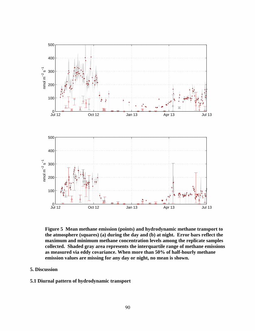
90

Figure 5 Mean methane emission (points) and hydrodynamic methane transport to the atmosphere (squares) (a) during the day and (b) at night. Error bars reflect the maximum and minimum methane concentration levels among the replicate samples collected. Shaded gray area represents the interquartile range of methane emissions as measured via eddy covariance. When more than 50% of half-hourly methane emission values are missing for any day or night, no mean is shown.

5. Discussion 5.1 Diurnal pattern of hydrodynamic transport

nmol

m−

2 s−

1

Jul 12 Oct 12 Jan 13 Apr 13 Jul 130

100

200

300

400

500

nmol

m−

2 s−

1

Jul 12 Oct 12 Jan 13 Apr 13 Jul 130

100

200

300

400

500

91

Nighttime hydrodynamic methane transport was more than two times daytime hydrodynamic transport on September 6, 2012 and on most of the 24 non-contiguous days water samples were collected. The ratio of nighttime to daytime hydrodynamic transport averaged 2.4. On one of the 24 days, temperature remained below 4 C over the entire day and daytime transport exceeded nighttime transport by a factor of 3. Because of the way we modeled hydrodynamic transport, these day-to-night differences in hydrodynamic transport reflect day-to-night differences in the gas transfer velocity k only. The relatively large day-to-night differences in k support our approach of accounting for variability in k while using a once-daily measurement of dissolved methane concentration. As described in section 3.4, on the two occasions when dissolved methane levels were measured multiple times over a single day, the percent difference between mean nighttime and mean daytime methane level was approximately 20%. The enhancement of hydrodynamic transport at night on most days is opposite the typical pattern of the other methane transport mechanisms. Ebullition increases during the day because of reduced methane solubility and density at higher temperatures (Fechner-Levy and Hemmond, 1996). Plant-mediated methane transport increases during the day because stomata are open and because of advection via humidity-induced pressurization within certain species of wetland plants (Bendix et al., 1992; Reid and Jaffe, 2012; Van der Nat et al., 1998). This partly explains the larger relative contribution of hydrodynamic transport to total methane emissions at night. During the day hydrodynamic transport is being overwhelmed by much larger emissions through plants and in bubbles. 5.2 Contribution of hydrodynamic transport to total methane emissions Integrating nighttime fluxes over the nearly year-long study period (while accounting for the changing duration of darkness) indicates that hydrodynamic transport contributes 54% of total methane emissions at night (Figure 6). Daytime hydrodynamic transport of methane amounts to only 18% of total daytime methane emissions. Integrating both daytime and nighttime data over the course of the study period suggests that 31% of net methane emissions can be attributed to the hydrodynamic transport of methane to the atmosphere.

92

Figure 6 Average methane emissions (dark red) and the contribution to methane emissions from hydrodynamic transport (light red) over the nearly year-long study period (19 July 2012 – 27 June 2013) at a temperate freshwater marsh. Error bars represent bootstrapped 95% confidence intervals of interpolated daytime and nighttime means for the study period.

The importance of hydrodynamic gas transport through the air-water interface to net fluxes observed at our marsh study site is likely also applicable to other marshes. Heat fluxes as strongly negative as -200 W m-2 have been observed in other marshes (e.g. Burba et al., 1999; Bidlake et al., 2000). The dissolved gas concentrations measured in the marsh study site are high but fall in the range of measurements from some wetlands in the literature (e.g. Sebacher et al., 1983; Happell et al., 1995). Therefore we expect that in many permanently flooded marshes, hydrodynamic transport is responsible for a significant portion of total methane fluxes. Nevertheless, our finding that hydrodynamic transport of methane is responsible for 31% of total methane emissions and 54% of nighttime fluxes at the marsh study contrasts sharply with the results of other studies. Others have found dissolved methane fluxes to be much smaller percentages of total methane emissions: 9% (Whiting et al., 1991), 8% (Morrissey and Livingston, 1992), 6% (Holzapfel-Pschorn et al., 1986; Chanton et al., 1993 and Whiting and Chanton, 1992), 3% (Chanton et al., 1992) or 2% (Van der Nat et al., 1998). These and other similar results have created the widespread perception that dissolved methane transport, including hydrodynamic transport, is negligible. However, because of the methods used in these studies, their results may not be representative of temporally-averaged, dissolved methane transport in wetlands with emergent vegetation. To isolate dissolved methane transport through the air-water interface from plant mediated transport, in these studies chambers were placed over areas of open water near emergent vegetation (e.g. Van der Nat et al., 1998) or between emergent plants (e.g. Chanton et al., 1993),

Day Night Total0

20

40

60

80

100

120

140

nmol

m−

2 s−

1

93

or where emergent vegetation had been clipped below the water surface (Holzapfel-Pschorn et al., 1986). Dissolved methane transport was measured from the rate of increase in methane concentration in the chamber over a few short intervals, usually during daylight hours. Emergent vegetation not only transports methane to that atmosphere; it also plays a key role in methane production by exuding labile carbon that serves as substrate for methanogenesis (Laanbroek, 2010). Differences in methane emissions between vegetated areas and unvegetated areas or areas where vegetation has been clipped below the water surface may reflect differences in methane production rather than the difference in transport rates. Furthermore, chambers are likely to interfere with thermal and wind-driven gas transport across the air-water interface, perhaps more than they interfere with transport through the gas filled tissue of wetland plants. Lastly, daytime chamber measurements probably overestimate 24-hour-average plant-mediated gas transport, because daytime plant-mediated transport tends to be higher during the day. On the other hand, daytime chamber measurements probably underestimate 24-hour average dissolved methane transport, because hydrodynamic transport has been shown here to be higher at night. Gas transfer velocity models (e.g. Equations 1 and 2) offer a non-intrusive method for isolating dissolved methane transport from other methane transport in wetlands with emergent vegetation. Chamber based investigations of the contribution of dissolved methane transport relative to plant-mediated transport have probably led to its being undercounted. 5.3 Implications for wetland methane modeling

Hydrodynamic transport, if integrated into wetland methane models, would likely impact predicted methane emissions. The developers of one global methane model, CLM4Me, tested the sensitivity of the model to an arbitrary ten-fold increase in the molecular diffusivity. The increased diffusivity was intended to represent advection within the soil. Stirring in surface water can enhance mixing above molecular diffusivity by many orders of magnitude (Fisher et al., 1979). The ten-fold increase in the molecular diffusivity resulted in a substantial decrease (25%) in tropical wetland methane emissions (Riley et al., 2011). Tropical methane emissions are important because they account for the majority of global methane emissions (Bloom et al., 2010). The sensitivity of a global methane model to a ten-fold increase in the molecular diffusivity suggests that enhanced transport due to stirring motions in the water column, including thermal convection, can strongly affect what percentage of produced methane reaches the surface. While wetland methane emissions contribute to global radiative forcing, this effect may be outweighed by wetland carbon sequestration even in the short term (Mitsch et al., 2013; Euliss et al., 2006; Chmura et al., 2003). This prospect has spurred interest in monetizing wetland carbon sequestration for trading in carbon markets in California (USA) and elsewhere. Carbon credits for wetland carbon sequestration have yet to be included in carbon markets, partly because of lingering questions about the extent to which wetland methane emissions detract from carbon storage. Improved models of wetland methane emissions could help determine the net impact of wetlands on global radiative forcing. 6. Summary

94

Here we applied results from a laboratory investigation of hydrodynamic dissolved gas transport in wetland surface water to a freshwater marsh and showed that the contribution of hydrodynamic methane transport to total methane emissions is surprisingly large. Thermal convection occurring as the marsh water surface cooled enhanced hydrodynamic dissolved methane transport such that it accounted for 54% of methane releases at night. Overall, hydrodynamic transport of dissolved methane was responsible for 31% annual methane emissions. Previous studies have assumed that dissolved methane transport occurs as molecular diffusion only and identified zero to negligible contribution. Our results suggest that a significant portion of methane transport to the atmosphere in wetlands may be neither plant-mediated nor due to ebullition. This is in contrast to a number of observational studies and the assumption of widely used methane models. Modifying the representation of dissolved methane transport to include hydrodynamic transport may affect predictions of both the timing of methane emissions and total emissions. It could also help to constrain model predictions of contemporary and future wetland methane emissions.

95

References

Arneth, A. et al. Terrestrial biogeochemical feedbacks in the climate system. Nat. Geosci. 3, 525-532 (2010). Aydin, M. et al., Recent decreases in fossil-fuel emissions of ethane and methane derived from firn air. Nature 476, 198-201 (2011). Baldocchi, D. D., Hincks, B. B. & Meyers, T. P. Measuring biosphere-atmosphere exchanges of biologically related gases with micrometeorological methods. Ecology 69, 1331-1340 (1988). Baldocchi, D. D. Assessing the eddy covariance technique for evaluating carbon dioxide exchange rates of ecosystems: past, present and future. Glob. Change Biol. 9, 479-492 (2003). Bendix, M., Tornbjerg, T., & Brix, H. Internal gas transport in Typha latifolia L. and Typha angustifolia L. 1. Humidity-induced pressurization and convective throughflow. Aquat. Bot. 49, 75-89 (1994). Bidlake, W. R. Evapotranspiration from a bulrush-dominated wetland in the Klamath Basin, Oregon, J. – Am. Water Works Assoc. 36, 1309-1320 (2000). Billesbach D. P. Estimating uncertainties in individual eddy covariance flux measurements: A comparison of methods and a proposed new method, Agr. Forest Meteorol. 151, 394-405 (2011). Bloom, A. A., Palmer, P. I., Fraser, A., Reay, D. S., & Frankenberg, C. Large-scale controls of methanogenesis inferred from methane and gravity spaceborne data. Science 327, 322-325 (2010). Bousquet, P. et al. Contribution of anthropogenic and natural sources to atmospheric methane variability. Nature 443, 439-443 (2006). Bridgham, S. D., Cadillo‐Quiroz, H., Keller, J. K. & Zhuang, Q. Methane emissions from wetlands: biogeochemical, microbial, and modeling perspectives from local to global scales. Glob. Change Biol. 19, 1325-1346 (2013). Burba, G. G., Verma, S. B. & Kim, J. Surface energy fluxes of Phragmites australis in a prairie wetland, Agr. Forest Meteorol. 94, 31-51 (1999). Chanton, J. P., Martens, C. S., Kelley, C. A., Crill, P. M., & Showers, W. J. Methane transport mechanisms and isotopic fractionation in emergent macrophytes of an Alaskan tundra lake. J. Geophys. Res. 97, 16681-16688 (1992). Chanton, J. P., Whiting, G. J., Happell, J. D., & Gerard, G. Contrasting rates and diurnal patterns of methane emission from emergent aquatic macrophytes. Aquat. Bot. 46, 111-128 (1993). Chmura, G. L., Anisfeld, S. C., Cahoon, D. R. & Lynch, J. C. Global carbon sequestration in tidal, saline wetland soils, Global Biogeochem. Cycles 17, 1111 (2003).

96

Detto, M., Verfaillie, J., Anderson, F., Xu, L., & Baldocchi, D. D. Comparing laser-based open-and closed-path gas analyzers to measure methane fluxes using the eddy covariance method. Agr. Forest Meteorol. 151, 1312-1324 (2011). Denman, K. L. et al. in Climate Change 2007: The Physical Science Basis. Contribution of Working Group I to the Fourth Assessment Report of the Intergovernmental Panel on Climate Change (eds by Solomon, S. et al.) 541-584 (Cambridge Univ. Press, 2007). Dinsmore, K. J., Billett, M. F., & Dyson, K. E. Temperature and precipitation drive temporal variability in aquatic carbon and GHG concentrations and fluxes in a peatland catchment. Glob. Change Biol. 19, 2133-2148 (2013). Euliss Jr, N.H. et al. North American prairie wetlands are important nonforested land-based carbon storage sites, Sci. Total Environ. 361, 179-188 (2006). Fechner-Levy, E. J. & Hemond, H. F. Trapped methane volume and potential effects on methane ebullition in a northern peatland, Limnol. Oceanogr. 41, 1375-1383 (1996). Fisher, H. B., List, E. J., Koh, R. C. Y., Imberger, J. & Brooks, N. H. Mixing in inland and coastal waters. New York: Academic Press, Inc (1979). Gedney, N., Cox, P. M. & Huntingford, C. Climate feedback from wetland methane emissions. Geophys. Res. Lett. 31, L20503 (2004). Godwin, C. M., McNamara, P. J. & Markfort, C. D. Evening methane emission pulses from a boreal wetland correspond to convective mixing in hollows. J. Geophys. Res.: Biogeosci. 118, 994-1005 (2013). Happell, J. D., Chanton, J. P. & Showers, W. J. Methane transfer across the water-air interface in stagnant wooded swamps of Florida: Evaluation of mass-transfer coefficients and isotopic fractionation, Limnol. Oceanogr. 40, 290-298 (1995). Holzapfel-Pschorn, A., Conrad, R. & Seiler, W. Effects of vegetation on the emission of methane from submerged paddy soil. Plant Soil 92, 223-233 (1986). Hope, D., Dawson, J. J., Cresser, M. S. & Billett, M. F. A method for measuring free CO2 in upland streamwater using headspace analysis. J. Hydrol. 166, 1-14 (1995). Heimann, M. Atmospheric science: Enigma of the recent methane budget. Nature 476, 157-158 (2011). Houghton, J. T. et al. Climate Change 2001: The Scientific Basis. Contribution of Working Group I to the Third Assessment Report of the Intergovernmental Panel on Climate Change (Cambridge Univ. Press, 2001).

97

Kai, F. M., Tyler, S. C., Randerson, J. T. & Blake, D. R. Reduced methane growth rate explained by decreased Northern Hemisphere microbial sources. Nature 476, 194-197 (2011). King, G. M. Regulation by light of methane emissions from a wetland. Nature 345, 513-515 (1990). Kling, G. W., Kipphut, G. W. & Miller, M. C. The flux of CO2 and CH4 from lakes and rivers in arctic Alaska. Hydrobiologia 240, 23-36 (1992). Laanbroek, H. J. Methane emission from natural wetlands: interplay between emergent macrophytes and soil microbial processes. A mini-review, Ann. Bot. 105, 141-153 (2010). Martynenko, O. G., & Khramtsov, P. P. Free-convective heat transfer: with many photographs of flows and heat exchange (Springer Verlag, 2005). Melton, J. R. et al. Present state of global wetland extent and wetland methane modeling: conclusions from the model inter-comparison project (WETCHIMP), Biogeosciences 10, 753-788, doi: 10.5194/bg-10-753-2013 (2013). Miller, R. L., Fram, M., Fujii, R. & Wheeler, G. Subsidence reversal in a re-established wetland in the Sacramento-San Joaquin Delta, California, USA, San Francisco Estuar. Watershed Sci. 6(3) (2008). Miller, R. L. & Fujii, R. Plant community, primary productivity, and environmental conditions following wetland re-establishment in the Sacramento-San Joaquin Delta, California, Wetlands Ecol. Manage. 18, 1-16 (2010). Miller, R. L. Carbon Gas Fluxes in Re-Established Wetlands on Organic Soils Differ Relative to Plant Community and Hydrology, Wetlands 31, 1055-1066, doi:10.1007/s13157-011-0215-2 (2011). Mitsch, W. J. et al. Wetlands, carbon, and climate change, Landscape Ecol. 28, 583-597 (2012). Montzka, S. A., Dlugokencky, E. J. & Butler, J. H. Non-CO2 greenhouse gases and climate change. Nature 476, 43-50 (2011). Moore, T. & Knowles, R. The influence of water table levels on methane and carbon dioxide emissions from peatland soils, Can. J. Soil Sci. 69, 33-38 (1989). Morrissey, L. A. & Livingston, G. P. Methane emissions from Alaska arctic tundra: An assessment of local spatial variability. J. Geophys. Res.: Atmos. 97, 16661-16670 (1992). Poindexter, C. M. & Variano, E. A. Gas exchange in wetlands with emergent vegetation: The effects of wind and thermal convection at the air‐water interface. Journal of Geophysical Research: Biogeosciences 118, 1297-1306 (2013).

98

Read, J. S. et al. Lake-size dependency of wind shear and convection as controls on gas exchange, Geophys. Res. Lett. 39, L09405, doi: 10.1029/2012GL051886 (2012). Reid, M. C. & Jaffé, P. R. Gas-phase and transpiration-driven mechanisms for volatilization through wetland macrophytes. Environ. Sci. Technol. 46, 5344-5352 (2012). Rettich, T. R., Handa, Y. P., Battino, R. & Wilhelm, E. Solubility of gases in liquids. 13. High-precision determination of Henry's constants for methane and ethane in liquid water at 275 to 328 K. J. Phys. Chem. 85, 3230-3237 (1981). Riley, W. J. et al. Barriers to predicting changes in global terrestrial methane fluxes: analyses using CLM4Me, a methane biogeochemistry model integrated in CESM, Biogeosciences 8, 1925–1953, doi: 10.5194/bg-8-1925-2011 (2011). Rojstaczer, S. & Deverel, S. J. Land subsidence in drained histosols and highly organic mineral soils of California. Soil Sci. Soc. Am. J. 59, 1162-1167 (1995). Sebacher, D. I., Harriss, R. C. & Bartlett, K. B. Methane flux from air-water interface: air velocity effects, Tellus, Ser. B 35, 103-109, doi: 10.1111/j.1600-0889.1983.tb00014.x (1983). Sebacher, D. I., Harriss, R. C., Bartlett, K. B., Sebacher, S. M. & Grice, S. S. Atmospheric methane sources: Alaskan tundra bogs, an alpine fen, and a subarctic boreal marsh. Tellus, Ser. B 38, 1-10 (1986). Sharifi, A., Kalin, L., Hantush, M. M., Isik, S. & Jordan, T. E. Carbon dynamics and export from flooded wetlands: A modeling approach. Ecol. Modell. 263, 196-210 (2013). Soloviev, A.,Donelan, M. Graber, H., Haus, B. & Schlüssel, P. An approach to estimation of near-surface turbulence and CO2 transfer velocity from remote sensing data, J. Marine Syst. 66, 182-194, doi: 10.1016/j.jmarsys.2006.03.023 (2007). Sorrell, B. K. & Boon, P. I. Convective gas flow in Eleocharis sphacelata R. Br.: methane transport and release from wetlands. Aquat. Bot. 47, 197-212 (1994). Van Der Nat, F. W. A., Middelburg, J. J., Van Meteren, D. & Wielemakers, A. Diel methane emission patterns from Scirpus lacustris and Phragmites australis, Biogeochemistry 41, 1-22 (1998). van Groenigen, K. J. Osenberg, C. W. & Hungate, B. A. Increased soil emissions of potent greenhouse gases under increased atmospheric CO2. Nature 475, 214-216 (2011). Walter, B. P. & Heimann, M. A process-based, climate sensitive model to derive methane emissions from natural wetlands, Global Biogeochem. Cycles 14, 745–65, doi: 10.1029/1999GB001204 (2000).

99

Webb, E. K., Pearman, G. I., Leuning, R. Correction of flux measurements for density effects due to heat and water vapor transfer, Q. J. Roy. Meteor. Soc. 106, 85-100 (1980). Weiss, R. Carbon dioxide in water and seawater: the solubility of a non-ideal gas. Mar. Chem. 2, 203-215 (1974). Whiting, G. J., Chanton, J. P., Bartlett, D. S. & Happell, J. D. Relationships between CH4 emission, biomass, and CO2 exchange in a subtropical grassland. J. Geophys. Res.: Atmos. 96, 13067-13071 (1991). Whiting, G. J. & Chanton, J. P. Plant‐dependent CH4 emission in a subarctic Canadian fen, Global Biogeochem. Cycles 6, 225-231 (1992). Whiting, G. J. & Chanton, J. P. Primary production control of methane emission from wetlands, Nature 364, 794-795 (1993).

100

Chapter 6 Conclusions Water flow, even in the shallow, relatively still wetland, remains important to air-water gas transfer. The usual forces behind gas transfer in other aquatic environments appear however to be less important in wetlands than surface-cooling-driven convection, a process often outweighed in oceans and lakes by wind-driven gas transfer. Wind-driven gas transfer in wetlands, which occurs in a unique spatial pattern due to the presence of emergent vegetation stems, contributes minimally to gas fluxes except when in-canopy wind speeds are high. The unusually high wind speed variance in vegetation canopies may amplify the wind’s effects on gas transfer in these conditions. The non-negligible effects of water flow in wetlands make it is essential to be able to characterize flow velocities accurately. Acoustic Doppler velocimeters, while susceptible to bias, can still be used with caution in wetlands. Two of the more direct implications of these conclusions are described below along with several research off-shoots that are suggested. Implications for wetland flow measurement Acoustic Doppler velocimeters have been used to measure mean flow in a number of wetlands (e.g. He et al., 2010; Harvey et al., 2009; Neumeier and Ciavola, 2004; Nepf and Oldham, 1997). The results of Chapter 3 suggest that some of these flow measurements include acoustic streaming bias. This bias affects measurements most when a component of the mean flow direction is oriented parallel to the axis of ADV probe. An ADV might be oriented this way when total water depth is smaller than the distance from the ADV probe to the sampling volume, 10 cm and 15 cm for Sontek and Nortek field ADV models, respectively. An investigation by He et al. (2010) into the drivers of flow in the Florida Everglades illustrates the difficulties with ADV flow measurement in wetlands given the acoustic streaming reported in Chapter 3. He et al. (2010) used a side-looking Sontek ADV to measure flow velocities and directions in the Everglades at multiple sites over a 5-year period. (A side-looking probe generates acoustic streaming in the horizontal.) Average daily water speeds never exceeded 0.03 m s-1 throughout the 5-year campaign, thus a reasonable choice for the nominal velocity range setting would have been ±0.10 m s-1. The experiments described in Chapter 3 revealed that for a Sontek ADV with the nominal velocity range setting set to ±0.10 m s-1, the spatial average acoustic streaming velocity in the sampling volume is 0.0071 m s-1. This velocity is 24% of the maximum daily average velocity measured in the Everglades by He et al. (2010), 0.03 m s-1. This velocity is more than 100% of the lowest seasonal average velocity observed, 0.0025 m s-1. For these smallest observed flow velocities, acoustic streaming may have reversed the apparent direction of flow. He et al. (2010) report that for flow speeds above 0.005 m s-1, the mean flow direction was generally southwest and aligned with the historic flow direction. Below 0.005 m s−1, the mean flow direction shifted at several sites and was more variable between sites. Both of these results point to potential acoustic streaming bias in these low flow measurements. Some of the options detailed in Chapter 3 for addressing ADV bias due to acoustic streaming could prove useful for future flow measurement campaigns in the Everglades. Variability in

101

mean flow direction would make it difficult to completely avoid the acoustic streaming bias caused by ADV models with side-looking probes. By orienting the ADV probe perpendicular to mean flow direction (if that direction is known a priori) the bias could be minimized. Alternatively, the bias could be measured in quiescent conditions and subtracted from measurements after data collection. Using a down-looking ADV could also minimize bias in horizontal velocity measurements. Nonetheless, for very shallow locations an ADV model with a shorter distance between the probe and the sampling volume (such as the Nortek Vectrino) would need to be used. Implications for wetland biogeochemical modeling A central finding of Chapter 4 and 5 is that wetland water flow does matter to wetland fluxes of oxygen, carbon dioxide and methane. This is particularly relevant to the field of wetland biogeochemical modeling. A substantial fraction of global wetland area is comprised of wetlands with no standing water and hence minimal hydrodynamic transport (e.g. tundra). However wetlands with surface water emit more methane and store more carbon per unit area (Moore and Knowles, 1989). Furthermore, inundation, as measured by remote sensing data, is a parameter often used to identify global wetland extent (e.g. Riley et al., 2011; Tian et al., 2010; Bohn and Lettenmaier, 2010). Notwithstanding the importance of wetlands with surface water, many modelers do not modify the governing equations they use to characterize gas concentration in wetland saturated soil when dealing with wetland surface water. For example, Wetland-DNDC, a wetland carbon model (Zhang et al., 2002), and CLM4Me, a global methane model (Riley et al., 2011), both treat transport through the surface water in the same way they treat transport through the soil pore water: as molecular diffusion. This treatment of wetland surface water in part stems from the way modeling of wetland carbon and methane developed. Many terrestrial biogeochemical models have simply been reworked to include wetlands. The structure of Wetland-DNDC was adopted from a model for upland forest carbon and nitrogen dynamics for example (Zhang et al., 2002). A one-dimensional wetland methane model developed by Walter and Heimann (2000) recognizes that molecular diffusion of gases in water is a very slow process, and thus excludes it entirely. Nonetheless, this model does not include any hydrodynamic transport. Walter and Heimann (2000) acknowledge that “the occurrence of turbulent diffusion in the standing water and its effect on transport and reoxidation of methane could be important at tropical sites in particular.” Evidence, including inverse modeling results and remote sensing data, points to tropical wetlands as the source for the majority of global wetland methane emissions (Melton et al., 2013). Yet few of the more recent wetland biogeochemical models account for any surface water mixing. The Wetland CH4 Inter-comparison of Models Project (WETCHIMP) (Melton et al., 2013) compared ten recently developed global methane models. Two of these models employ the Walter and Heimann (2000) model for the calculation of methane emissions, UW-VIC (Bohn and Lettenmaier, 2010) and ORCHIDEE (Wania et al., 2012) and also exclude hydrodynamic transport. Two of the WETCHIMP models include hydrodynamic transport in the water column, but assume a constant value for the gas transfer velocity not tied to any particular driving force. The Dynamic Land Ecosystem Model (DLEM) uses the average gas transfer velocity measured

102

in a Florida swamp by Happell and Chanton (1995) of 3.47 x 10-6 m s-1 (1.25 cm hr-1) to quantify the diffusive transport across the air-water interface (Tian et al., 2010). The LPJ-Wetland Hydrology and Methane (LPJ-WHyMe) model uses a constant value of 5.75 x 10-6 m s-1 (2.07 cm hr-1) to quantify diffusive transport across the air-water interface (Wania et al., 2010). This value in the LPJ-WHyMe model is derived from Cole and Caraco’s (1998) model for lake gas

transfer as a function of wind speed: 7.110600 215.007.2 Uk . In LPJ-WHyMe, wind speed is

assumed to be effectively zero within the wetland vegetation canopy and the value of k600 in the Cole and Caraco (1998) model at zero wind speed is used. If the average k600 value predicted in Chapter 5 for the restored wetlands on Twitchell Island (1.2 x 10−6 m s-1 or 0.43 cm hr-1) is representative, hydrodynamic transport may actually be overestimated in these two models. The developers of an additional WETCHIMP model, CLM4Me, tested the effect of an enhancement factor of ten applied to the molecular diffusivity. This enhancement factor was intended to simulate convective transport in the soil but was not included in their baseline results. The exclusion of hydrodynamic transport in some wetland biogeochemical models has the potential to skew modeling results. Interfacial transport of oxygen from the atmosphere to the water column beyond the transport predicted by molecular diffusion could lead to increased methane consumption in the surface water. Hydrodynamic transport diverts methane away from plant aerenchyma and ebullition, two more rapid routes to the atmosphere on which there is less possibility for methane oxidation. Inclusion of a ten-fold enhancement factor for the molecular diffusivity resulted in a more than 25% reduction in annual methane emissions in the CLM4Me model (Riley et al., 2011). Because of the many other differences between the WETCHIMP models it is difficult to pinpoint the effect of the integration of hydrodynamic transport in LPJ-WHyMe and DLEM by comparing them to other WETCHIMP models. One of the most striking findings of WETCHIMP is the consistent prediction across all ten models of substantially increased methane emissions when the atmospheric CO2 level is set to 857 ppm, the level predicted under some scenarios for the year 2100. The average increase in wetland methane emissions predicted over the ten models is greater than 50% (Melton et al., 2013). This finding underlines the importance of wetland biogeochemical modeling for predicting future climate change and climate change feedbacks and the importance of accurately representing the mechanisms involved in wetland gas fluxes in these models. Next steps Future work I would like to pursue based on the results of Chapters 3-5 includes (1) direct measurements of gas transfer velocity and water flow at the restored wetlands on Twitchell Island, (2) experiments to determine the effects of horizontally heterogeneous vegetation cover on the gas transfer velocity, (3) experiments on the effect of water column stirring on carbon sequestration and methane emissions in wetland mesocosms, and (4) additional Particle Image Velocimetry (PIV) measurements to assess the role of the heat fluxes and surfactants on surface divergence near and far from plant stems. Several factors raise the possibility that gas transfer velocity at the Twitchell Island wetlands are different than in the model wetland in the laboratory used in Chapter 4. Small floating plants specifically Lemna spp. (duckweed) often covers portions of the water surface at the restored

103

wetlands on Twitchell Island. These plants may affect gas transfer velocity directly by acting as a physical barrier. These plants may also act indirectly on gas transfer by damping the effects of wind shear or inhibiting latent heat loss. While wind shear and surface cooling are likely to be important drivers of gas transfer in this wetland, other processes such as seiches and currents could also be important. The mean current through this wetland from inflow to outflow is on the order of tenths of millimeters per second, but short-circuiting could result in regions of faster velocity. A short ADV deployment in the wetland revealed periodic velocities on the order of millimeters per second in the restored wetland on Twitchell Island that could be due to seiching. A direct measurement of the gas transfer velocity via dual tracer release along with velocity profiles at various locations throughout the wetland would help verify the accuracy of the lab-based models for gas transfer velocity of Chapter 4 in this restored wetland. New wetlands planned in the interest of subsidence reversal on Twitchell Island will be of a different design than the wetland described in Chapter 5. These new wetlands, rather than being nearly uniformly colonized by emergent vegetation, will have areas of open water too deep for emergent plants. (A recently restored wetland in Sacramento-San Joaquin Island on Sherman Island is also of this design.) A primary motivation for this design is the need for oxygenated water to support fish for mosquito control (Bryan Brock of the California Department of Water Resources, Personal Communication, 23 October 2012). The addition of open water zones will enhance wetland water column stirring, and in turn gas transfer, via a number of processes. Differential heating and cooling of the wetland will drive lateral currents between vegetated and open water regions. Higher wind speeds above the air-water interface in open water regions will generate currents and waves. The propagation of wind-driven currents and waves into vegetated zones will lead to gradients in the gas transfer velocity in these zones. Wind-driven gas transfer will be smallest in interior regions of vegetated zones and higher at the edges of vegetated zones. The ratio of vegetated area to open water area and the configuration of vegetated area, whether concentrated or distributed will thus affect net gas transfer. Experiments to determine how gas transfer velocity varies within the emergent vegetation with proximity to open water could prove valuable in guiding the design of additional wetlands for subsidence reversal. Spatial variability of water column stirring will lead to variability in the gas transfer velocity and air-water transport of CO2 and CH4. Spatial variability of water column stirring may also lead to variability in the production of CO2 and CH4. Therefore, it might be interesting to investigate the role of water column stirring on net wetland carbon and methane fluxes in a more controlled environment such as wetland mesocosms. Wetland stirring could be controlled and varied across otherwise identical mesocosms, for example via different strength submersible pumps. Net fluxes of carbon and methane from each mesocosm could be measured to determine the effect on wetland carbon sequestration and methane emissions. Increased stirring would increase oxygen availability, which would amplify aerobic respiration of organic matter and inhibit methane production. Thus increased stirring probably results in reduced carbon sequestration and reduced methane emissions. Still an experiment like this could be useful to confirm these effects. Finally, to help clarify the mechanisms of air-water gas exchange in wetlands, PIV measurements in the model wetland in the laboratory referenced in Chapter 4 could be expanded. For the measurements described in Chapter 4, which identified small regions of high surface divergence around plant stems at high wind speed, water temperatures needed for the

104

determination of heat into (or out of) the water column were not measured. Questions then remain about the influence of surface cooling and heating on the surface divergence, both far from the stems and in the region of high surface divergence near the stems. Additional PIV and temperature measurements could indicate that surface divergence away from stems reflects (1) thermal convective motions or (2) residual effects of flows around plant stems or (3) wind-driven motions unrelated to flows around plant stems. Limited PIV data collected after first skimming the water surface revealed that surface divergence was highest upwind of stem faces, lowest in the large wakes downwind of stems and of intermediate value far from stems. Mean values of the surface divergence in each of these regions were not established. Additional PIV measurements with prior surface skimming could be used establish whether these larger plant wakes present when surfactants are absent are important to the gas transfer velocity. References Bohn, T. J. and D. P. Lettenmaier (2010), Systematic biases in large‐scale estimates of wetland methane emissions arising from water table formulations, Geophys. Res. Lett. 37(22), L22401, doi: 10.1029/2010GL045450. Cole, J.J. and N.F. Caraco (1998), Atmospheric exchange of carbon dioxide in a low-wind oligotrophic lake measured by the addition of SF6, Limnol. Oceanogr. 43(4), 647-56. He, G., V. Engel, L. Leopard, A. Croft, D. Childers, M. Laas, Y. Deng and H. M. Solo-Gabriele (2010), Factors controlling surface water flow in a low-gradient subtropical wetlands, Wetlands 30, 275-286, DOI 10.1007/s13157-010-0022-1. Melton, J. R., R. Wania, E. L. Hodson, B. Poulter, B. Ringeval et al. (2013), Present state of global wetland extent and wetland methane modeling: conclusions from the model inter-comparison project (WETCHIMP), Biogeosciences 10, 753-788, doi: 10.5194/bg-10-753-2013. Moore, T. and R. Knowles (1989), The influence of water table levels on methane and carbon dioxide emissions from peatland soils, Can. J. Soil Sci. 69(1), 33-38. Nepf, H. M. and C. E. Oldham (1997), Exchange dynamics of a shallow contaminated wetland, Aquat. Sci. 59(3), 193-213. Neumeier, U. and P. Ciavola (2004), Flow resistance and associated sedimentary processes in a Spartina maritima salt-marsh, J. Coast. Res. 202, 435-447. Riley, W. J., Z. M. Subin, D. M. Lawrence, S. C. Swenson, M. S. Torn, L. Meng, N. M. Mahowald, and P. Hess (2011), Barriers to predicting changes in global terrestrial methane fluxes: analyses using CLM4Me, a methane biogeochemistry model integrated in CESM, Biogeosciences 8, 1925–1953, doi: 10.5194/bg-8-1925-2011. Tian, H., X. Xu, M. Liu, W. Ren, C. Zhang, G. Chen, and C. Lu (2010), Spatial and temporal patterns of CH4 and N2O fluxes in terrestrial ecosystems of North America during 1979–2008:

105

application of a global biogeochemistry model, Biogeosciences 7, 2673–2694, doi: 10.5194/bg-7-2673-2010. Walter, B. P. and M. Heimann (2000), A process-based, climate sensitive model to derive methane emissions from natural wetlands, Global Biogeochem. Cycles 14(3), 745–65, doi: 10.1029/1999GB001204. Wania, R., J. Melton, E. Hodson, B. Poulter, B. Ringeval, R. Spahni, T. Bohn, C. Avis, G. Chen, and A. Eliseev (2012), Present state of global wetland extent and wetland methane modelling: methodology of a model intercomparison project (WETCHIMP), Geosci. Model Dev. Discuss. 5, 4071-4136. Wania, R., I. Ross, and I. Prentice (2010), Implementation and evaluation of a new methane model within a dynamic global vegetation model: LPJ-WHyMe v1.3.1, Geosci. Model Dev. Discuss. 3, 565-584. Zhang, Y., C. Li, C.C. Trettin, H. Li & G. Sun (2002), An integrated model of soil, hydrology, and vegetation for carbon dynamics in wetland ecosystems, Global Biogeochem. Cycles 16(4), 1061-77, doi: 10.1029/2001GB001838.