What are the welfare effects of fishery policies?

Jonathan Sweeney

SEEP, March 7, 2016

Outline

• Background

• Setting

• Market model

• Welfare model

• Policy comments

• Extensions

Outline

• Background

• Setting

• Market model

• Welfare model

• Policy comments

• Extensions

Hawaii’s longline fishery

Species Mean Annual Value (dollars) SE Annual Value (dollars) Mean Annual Catch (lbs) SE Annual Catch (lbs)

Bigeye Tuna41,658,624 3,758,148 9,779,828 396,010

Broadbill Swordfish5,256,164 785,098 1,633,736 260,199

Yellowfin Tuna4,930,470 443,995 1,529,837 84,999

Opah2,198,574 192,900 1,363,067 118,283

Mahi Mahi1,652,181 132,109 763,298 35,895

Tombo1,453,473 203,461 803,191 92,067

Monchong1,378,601 136,105 606,910 52,414

Striped Marlin1,133,529 76,757 731,574 85,126

Ono951,230 66,058 377,374 23,903

Blue Marlin757,974 53,463 501,246 16,951

Common pool resource problem

http://www.fao.org/docrep/003/v8400e/v8400E02.htm

Endangered species interactions

http://www.pifsc.noaa.gov/library/pubs/tech/NOAA_Tech_Memo_PIFSC_30.pdf

Management solutions in Hawaii

• Commercial fishing license

• Annual catch limits

• Restrict endangered species interactions

Management solutions in Hawaii

• Commercial fishing license

• Annual catch limits

• Restrict endangered species interactions

Management outcomes

• Race-to-fish behavior

• Closures

What are the welfare effects?

http://archives.starbulletin.com/2000/07/13/news/story3.html

Outline

• Background

• Setting

• Market model

• Welfare model

• Policy comments

• Extensions

Marshall’s market

Alfred Marshall, Principles of Economics

Honolulu fish auction

Honolulu fish auction

• Open daily except Sunday

• Unloading starts at 1am, open until all the fish are sold

• Prices set through a bidding process between wholesalers

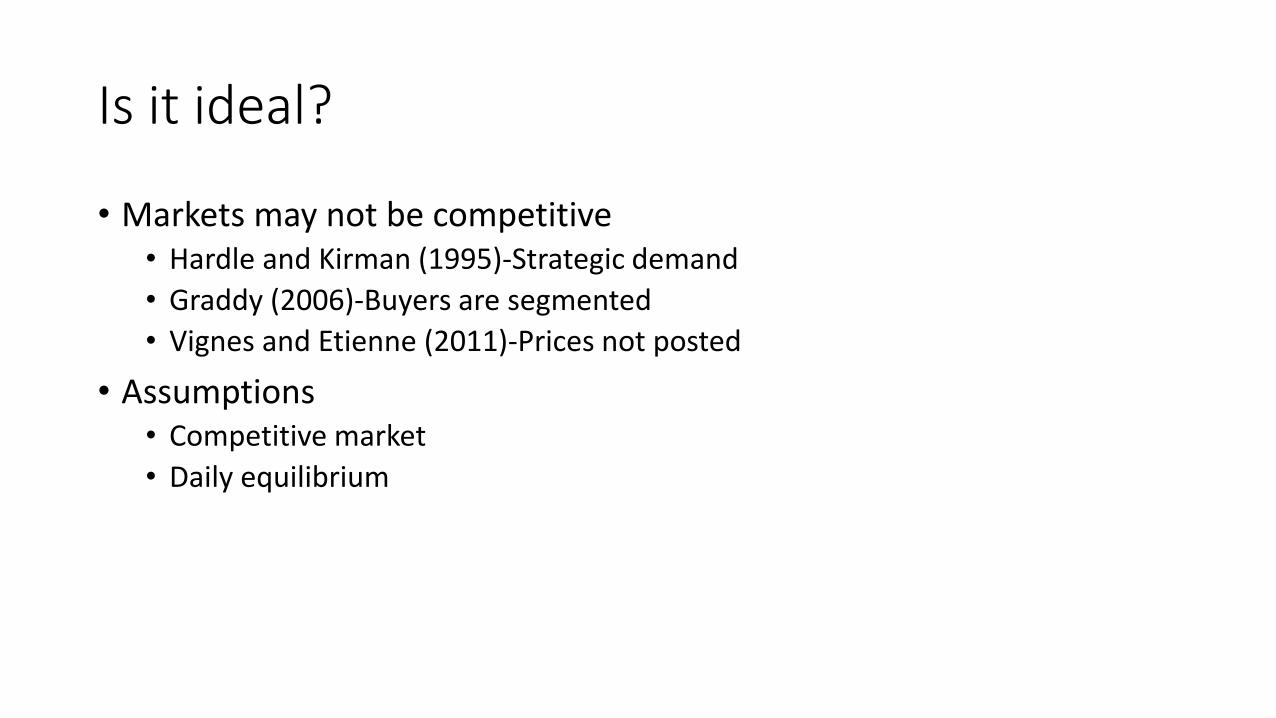
Is it ideal?

• Markets may not be competitive• Hardle and Kirman (1995)-Strategic demand

• Graddy (2006)-Buyers are segmented

• Vignes and Etienne (2011)-Prices not posted

• Assumptions• Competitive market

• Daily equilibrium

Market data

• Daily average price by fish species

• Daily sum quantity by fish species

• Focus on three most valuable species

Price and quantity

Time trends (Bigeye)

Time trends (Yellowfin)

Time trends (Swordfish)

Outline

• Background

• Setting

• Market model

• Welfare model

• Policy comments

• Extensions

Previous literature

• Studies of both supply and demand• Kahn and Kemp (1985)

• Huang et al. (2012)

• Studies of only demand side• Burton (1992)

• Hardle and Kirman (1995)

• Angrist et al. (2000)

• Hammarlund (2015)

• Huang (2015)

Our contribution

• Consistently estimate both supply and demand elasticities for fish

• Apply these estimates to accurately measure welfare effects from policies

Supply and demand

Supply of i:𝑞𝑖𝑠 = 𝛽0 + 𝛽1𝑝𝑖 + 휀

Demand for i:𝑞𝑖𝑑 = 𝛽3 + 𝛽4𝑝𝑖 + 휀

Wright (1928)

• Developed the instrumental variables estimator (IV)

• Find two instruments: one that shifts supply but not demand, the other shifts demand but not supply.

Examples

• Angrist et al. (2000)• Marine weather shifts fish supplied, but not fish demanded.

• Roberts and Schlenker (2013)• Weather shocks shifts agricultural supply but not demand

• Past yield shocks shift agricultural demand but not supply.

Our instruments

• Marine weather shifts supply but not demand• Wave height

• Price of substitutes shifts demand but not supply• Price of swordfish

• Price of bigeye

Instrument validation

• Must be relevant

• Must be exogenous

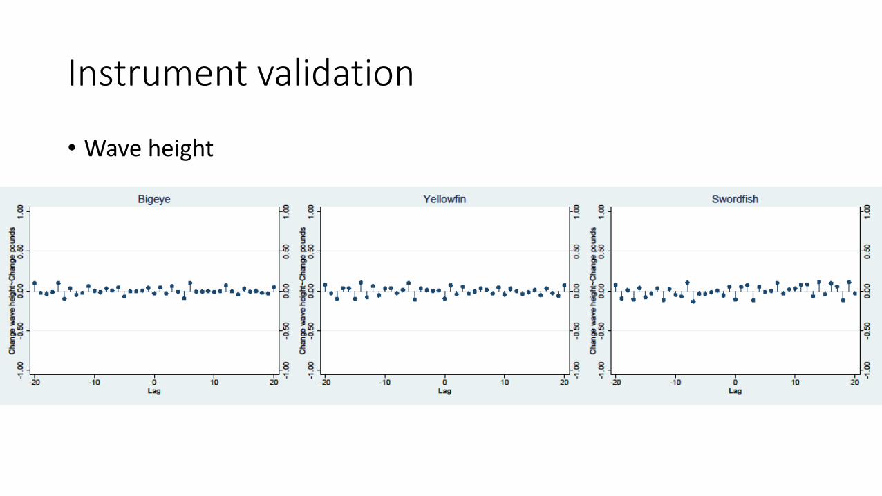
Instrument validation

• Wave height

Instrument validation

• Price of substitute

Trip Type YF (lbs) BE (lbs) SF (lbs)Tuna (D) 1101.08 (1719.96) 7076.88 (4822.13) 244.034 (579.829)Swordfish (S) 130.039 (395.567) 470.413 (956.967) 9303.64 (8784.01)

Supply and demand IV model

Supply i:𝑙𝑜𝑔𝑞𝑖

𝑠 = 𝛽0 + 𝛽1𝑙𝑜𝑔𝑝𝑖 + 𝛽2𝑥 + 휀𝑙𝑜𝑔𝑝𝑖 = 𝛿0 + 𝛿1𝑙𝑜𝑔𝑝−𝑖 + 𝛿2𝑥 + 𝜂

Demand i:𝑙𝑜𝑔𝑞𝑖

𝑑 = 𝛽3 + 𝛽4𝑙𝑜𝑔𝑝𝑖 + 𝛽5𝑥 + 휀𝑙𝑜𝑔𝑝𝑖 = 𝛿3 + 𝛿4𝑙𝑜𝑔𝑧 + 𝛿5𝑥 + 𝜂

i={bigeye, yellowfin, swordfish}

Estimation results

Bigeye (BE) Yellowfin (YF) Swordfish (SF)

Supply (qS) Demand (qD) Supply (qS) Demand (qD) Supply (qS) Demand (qD)

Price (psp) 2.79 (1.22) -2.71 (0.43) -0.52 (0.41) -13.83 (6.22) 6.98 (2.47) -3.66 (1.09)

Year FE Yes Yes Yes Yes Yes Yes

1st Stage

F-stat 12.17 35.73 42.51 4.70 12.17 24.14

N 3,548 3,430 3,531 3,410 3,548 1,256

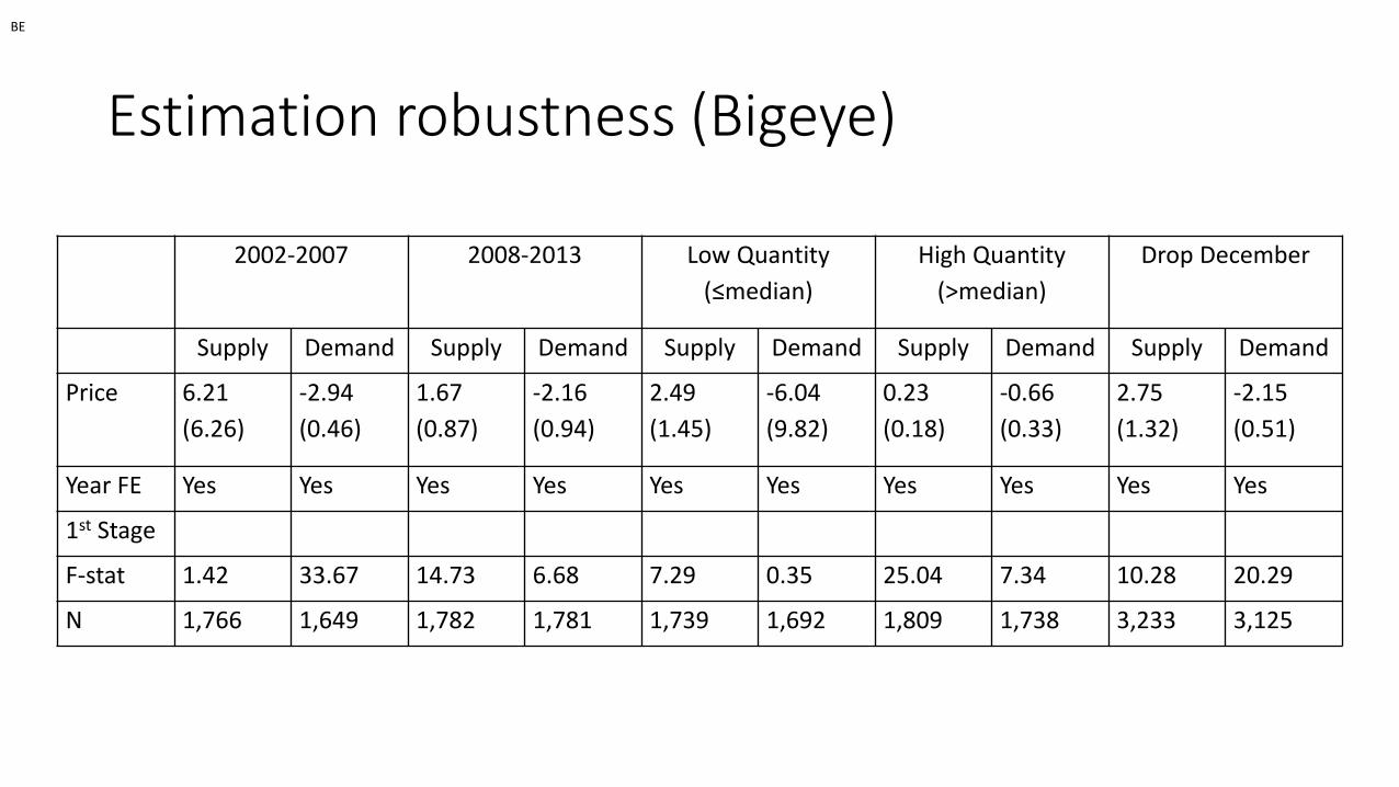
Estimation robustness (Bigeye)

2002-2007 2008-2013 Low Quantity

(≤median)

High Quantity

(>median)

Drop December

Supply Demand Supply Demand Supply Demand Supply Demand Supply Demand

Price 6.21

(6.26)

-2.94

(0.46)

1.67

(0.87)

-2.16

(0.94)

2.49

(1.45)

-6.04

(9.82)

0.23

(0.18)

-0.66

(0.33)

2.75

(1.32)

-2.15

(0.51)

Year FE Yes Yes Yes Yes Yes Yes Yes Yes Yes Yes

1st Stage

F-stat 1.42 33.67 14.73 6.68 7.29 0.35 25.04 7.34 10.28 20.29

N 1,766 1,649 1,782 1,781 1,739 1,692 1,809 1,738 3,233 3,125

BE

Estimation robustness (Yellowfin)

2002-2007 2008-2013 Low Quantity

(≤median)

High Quantity

(>median)

Drop December

Supply Demand Supply Demand Supply Demand Supply Demand Supply Demand

Price 0.31

(1.24)

-5.72

(2.16)

-0.79

(0.39)

-74.63

(200.4)

-1.66

(0.83)

-173.28

(2373.36)

0.45

(0.26)

-4.75

(8.52)

-0.79

(0.47)

-15.39

(8.61)

Year FE Yes Yes Yes Yes Yes Yes Yes Yes Yes Yes

1st Stage

F-stat 5.06 7.02 50.80 0.14 11.11 0.01 30.95 0.29 33.78 3.05

N 1,757 1,637 1,774 1,773 1,736 1,761 1,795 1,649 3,216 3,105

Estimation robustness (Swordfish)

2002-2007/2009-

2010

2008-2013/2011-

2013

Low Quantity

(≤median)

High Quantity

(>median)

Drop December

Supply Demand Supply Demand Supply Demand Supply Demand Supply Demand

Price 17.38

(14.96)

-6.66

(4.56)

3.53

(1.64)

-2.99

(1.05)

-1.11

(0.60)

1.34

(0.97)

0.10

(0.84)

4.25

(2.52)

6.97

(2.67)

-3.66

(1.09)

Year FE Yes Yes Yes Yes Yes Yes Yes Yes Yes Yes

1st Stage

F-stat 1.42 2.06 14.73 26.39 17.88 4.79 11.42 5.10 10.28 24.14

N 1,766 430 1,782 826 1,778 586 1,770 670 3,233 1,256

Outline

• Background

• Setting

• Market model

• Welfare model

• Policy comments

• Extensions

Marshall model

Invert supply and demand elasticity

𝑞 = 𝛽𝑝𝑝 + 휀

p= 𝛽𝑞𝑞 + 휀

𝛽𝑝 =𝑐𝑜𝑣(𝑞, 𝑝)

𝑣𝑎𝑟(𝑝)

𝛽𝑞 =𝑐𝑜𝑣(𝑝, 𝑞)

𝑣𝑎𝑟(𝑞)

Direct supply and demand elasticities

• BE:• Supply 0.65

• Demand -0.60

• SF:• Supply 0.37

• Demand -0.17

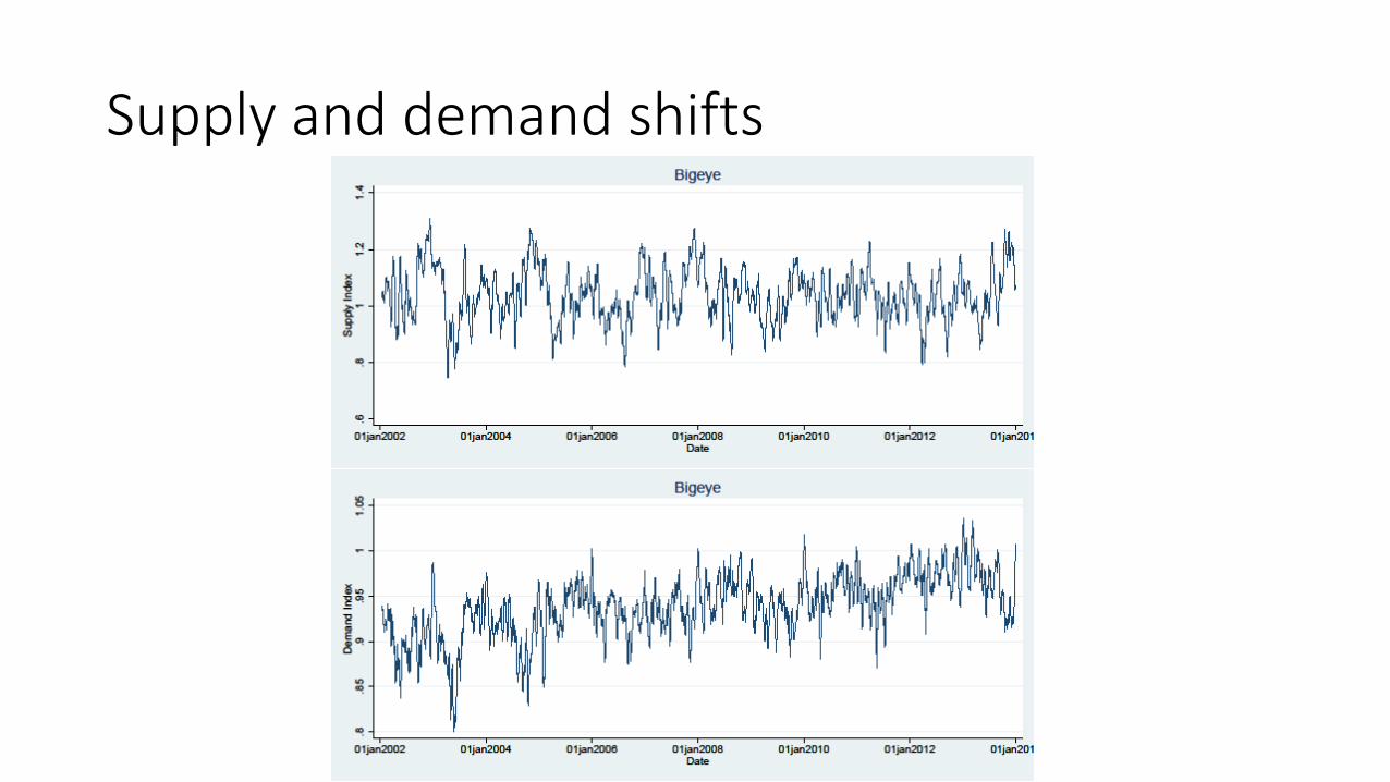
Supply and demand shifts

Supply and demand shifts

Measuring producer and consumer surplus

• By aggregating days, our index accounts for race-to-fish effects

• Log scaled index

Producer and consumer surplus index

Producer and consumer surplus index

Outline

• Background

• Setting

• Market model

• Welfare model

• Policy comments

• Extensions

Policy comments

• The effects of policies are not that large.

• Policies may in fact benefit producers and consumers.

• Interesting to see if trends continue

Response to anecdotes

• Closures drive consumers to imports.• These results suggest this is not the case. We observe the opposite effect.

• Decline in swordfish is driven by a change in consumers tastes.• In fact, we see a modest increase in demand.

• Decreases in supply seem to be the driver.

Outline

• Background

• Setting

• Market model

• Welfare model

• Policy comments

• Extensions

True welfare measure

• We estimate ordinary demand q=g(x,p)

• Need compensated demand q=h(u,p)

Vartia (1983)

• Develops algorithm to generate compensated demand from uncompensated.

True consumer and producer welfare

• Apply Vartia (1983) algorithm to estimate true consumer surplus.

• Extend his algorithm to estimate true producer surplus.

Thank you.