what can we learn about neighborhood effects...
TRANSCRIPT
144 AJS Volume 114 Number 1 (July 2008): 144–88
� 2008 by The University of Chicago. All rights reserved.0002-9602/2008/11401-0005$10.00
What Can We Learn about NeighborhoodEffects from the Moving to OpportunityExperiment?1
Jens LudwigUniversity of Chicago
Jeffrey B. LiebmanHarvard University
Jeffrey R. KlingBrookings Institution
Greg J. DuncanUniversity of California, Irvine
Lawrence F. KatzHarvard University
Ronald C. KesslerHarvard Medical School
Lisa SanbonmatsuNational Bureau of Economic Research
Experimental estimates from Moving to Opportunity (MTO) showno significant impacts of moves to lower-poverty neighborhoods onadult economic self-sufficiency four to seven years after randomassignment. The authors disagree with Clampet-Lundquist andMassey’s claim that MTO was a weak intervention and thereforeuninformative about neighborhood effects. MTO produced largechanges in neighborhood environments that improved adult mentalhealth and many outcomes for young females. Clampet-Lundquistand Massey’s claim that MTO experimental estimates are plaguedby selection bias is erroneous. Their new nonexperimental estimatesare uninformative because they add back the selection problemsthat MTO’s experimental design was intended to overcome.
INTRODUCTION
Experimental analyses of the data from the “interim evaluation” of theDepartment of Housing and Urban Development’s Moving to Oppor-
1 Support for this research was provided by grants from the National Science Foun-dation to the National Bureau of Economic Research (9876337 and 0091854) and theNational Consortium on Violence Research (9513040), as well as by the U.S. Depart-ment of Housing and Urban Development (HUD), the National Institute of Child
MTO Symposium: What Can We Learn from MTO?
145
tunity (MTO) housing mobility experiment, which measured outcomesfor participating adults and children four to seven years after randomassignment, find no significant impacts on adult economic outcomes fromthe opportunity to move to lower-poverty neighborhoods (Orr et al. 2003;Kling, Liebman, and Katz 2007). In an article in this issue, Susan Clampet-Lundquist and Douglas Massey (hereafter “CM”) reassess the MTOexperimental estimates and present new nonexperimental estimates ofneighborhood impacts on economic self-sufficiency.
We are delighted that CM have undertaken a reanalysis of data fromthe MTO interim evaluation. One of our teams’ key goals in partneringwith HUD and Abt Associates to fund, design, and implement the interimMTO study was to contribute to the research infrastructure available forstudying neighborhood effects. A discussion about what the MTO dataimply about neighborhood effects is exactly the type of exchange we hopedreanalysis of the MTO data would engender. We are particularly pleasedthat this reanalysis has been carried out by CM, since Clampet-Lundquisthas previously collaborated with two members of our team (Duncan andKling) on qualitative studies of MTO adult employment and the behaviorof young people, and we hold Massey in the highest esteem for his manydistinguished scholarly contributions.
The basic arguments developed by CM are as follows: MTO was aweak intervention for studying neighborhood effects because the exper-iment was focused on generating residential integration by social classrather than by both class and race. The low-poverty but predominantlyminority neighborhoods into which most MTO movers relocated are notcapable of producing substantial improvements in the economic outcomesof MTO families. Moreover, the fact that many families who were offeredthe chance to relocate through the MTO program did not do so, and thatsome MTO movers subsequently moved to higher-poverty areas on their
Health and Development and the National Institute of Mental Health (R01-HD40404and R01-HD40444), the Robert Wood Johnson Foundation, the Russell Sage Foun-dation, the Smith Richardson Foundation, the MacArthur Foundation, the W. T. GrantFoundation and the Spencer Foundation. Additional support was provided by grantsto Princeton University from the Robert Wood Johnson Foundation and from NICHD(5P30-HD32030 for the Office of Population Research), by the Princeton IndustrialRelations Section, the Bendheim-Thomas Center for Research on Child Wellbeing, thePrinceton Center for Health and Wellbeing, the National Bureau of Economic Re-search, and a Brookings Institution fellowship supported by the Andrew W. Mellonfoundation. Thanks to Susan Clampet-Lundquist, David Deming, Lisa Gennetian,Harold Pollack, and seminar participants at the University of Chicago, Harvard, andthe Population Association of America meetings for helpful comments and assistance.The MTO data used in this article are from HUD. The contents of this comment arethe views of the authors and do not necessarily reflect the views or policies of HUDor the U.S. government. Direct correspondence to Jens Ludwig, University of Chicago,969 East 60th Street, Chicago, Illinois 60637. E-mail: [email protected]
American Journal of Sociology
146
own, compromises the demonstration’s experimental design by impartingselection bias to estimates of the MTO intervention’s effects. CM’s newnonexperimental analysis of the MTO data suggests a substantial positive“association” between time spent in low-poverty neighborhoods and adulteconomic outcomes which, combined with evidence from other research,makes it likely that neighborhoods do have important impacts on theseoutcomes.
We respectfully disagree with each of the main methodological andsubstantive points developed by CM. To date, most of our team’s writingson MTO have focused on presenting and interpreting the main experi-mental impacts of the demonstration.2 We have not discussed in print anyof the broader questions raised by CM’s article about alternative researchmethodologies or more fundamental implications of the MTO evaluationfor theories of neighborhood effects. So we are grateful to the editor ofAJS for giving us the opportunity to discuss these issues.
In what follows, we address three main points. First, we clarify whatcan and cannot be learned from a randomized policy experiment withpartial compliance. We show that features of MTO that lead to what CMdescribe as “selection bias” do not bias estimates from a properly executedexperimental analysis of the MTO data. Their claim seems to reflect somemisunderstanding about the calculation of experimental estimates or whatis conventionally meant by selection bias. We focus on two types of es-timates that follow from MTO’s experimental design—termed “intent totreat” and “treatment on the treated” in the experimental literature.Roughly speaking, the MTO intent-to-treat (ITT) effect on a given out-come is the simple difference between the outcome for all individualsassigned at random to MTO’s experimental condition, regardless ofwhether they “complied” by actually moving through MTO to a low-poverty neighborhood, and the outcome for all individuals assigned tothe control group. In contrast, the treatment-on-the-treated (TOT) esti-mates are of outcome differences for families actually moving in con-junction with the program. We show that neither ITT nor TOT estimatesare biased by the fact that only some families moved through MTO orby the fact that not all movers stayed in low-poverty areas. Both esti-mators are informative about the existence of neighborhood effects onbehavior, contrary to the distinction CM make between estimating “policytreatment effects” and “neighborhood effects.”
2 For results derived from the interim MTO evaluation, see Orr et al. (2003), Kling,Ludwig and Katz (2005), Sanbonmatsu et al. (2006), Kling et al. (2007), and Ludwigand Kling (2007). Various members of our team were also involved in studying MTOparticipants from individual demonstration sites over the short term (see Katz, Kling,and Liebman 2001; Ludwig, Duncan, and Hirschfield 2001; Ludwig, Ladd, and Duncan2001; and Ludwig, Duncan, and Pinkston 2005).

MTO Symposium: What Can We Learn from MTO?
147
Second, we discuss whether the neighborhood differences generated byMTO are large enough to tell us anything useful about neighborhoodeffects. We show that CM’s classification of neighborhoods into “low” and“high” poverty groups on the basis of a single 20% poverty rate thresholdoverstates the degree to which subsequent mobility by families movingthrough the MTO program waters down the MTO “treatment dose.”Despite subsequent mobility, the average neighborhood environments offamilies moving through the program differed greatly from the neigh-borhoods of their control-group counterparts in terms of neighborhoodsocioeconomic status (SES), crime, and collective efficacy, but not in termsof race.
What to make of the limited MTO impacts on neighborhood racialintegration? CM argue that because these new communities are lowerpoverty but still overwhelmingly minority, they should not be expectedto change the behavioral outcomes of MTO families. This claim seemsinconsistent with the original theories of neighborhood effects that mo-tivated the MTO experiment, such as that of Wilson (1987), and also withevidence of sizable MTO impacts on other important outcomes, includingmental health, some indicators of physical health, and violent behavioramong adolescents (Kling et al. 2005; Kling et al. 2007). Perhaps one mightargue that moving to a neighborhood that is both low poverty and ma-jority white non-Hispanic is particularly important for improving eco-nomic outcomes. But that argument is inconsistent with CM’s newnonexperimental estimates, which, if taken at face value, suggest that theeffects on economic outcomes of living in segregated versus integratedlow-poverty tracts are indistinguishable.
The third point of our article is to consider whether anything usefulcan be learned about neighborhood effects from the new nonexperimentalestimates presented by CM. The answer, in our judgment, is no. We aresympathetic to CM’s goal of understanding how the effects of MTO varyby time spent in low-poverty neighborhoods. In any experiment, somesubjects will benefit more than others. Understanding how and why ben-efits vary across program participants can help inform policy design. ButCM’s approach reintroduces all of the selection problems that MTO’srandomization was designed to overcome.
Even taken at face value, the associations CM document are overstated,because their analysis confounds cohort and time effects with neighbor-hood effects, and they perform the wrong hypothesis test for determiningwhether extra time spent in a low- rather than high-poverty area improvesadult economic outcomes. CM measure economic outcomes at a singlepoint in time using data from the interim MTO survey. Random assign-ment occurred over the four-year period between 1994 and 1998. Ourprevious work suggests that earlier cohorts of movers may have benefited

American Journal of Sociology
148
more than later cohorts with respect to some outcomes, even when timesince random assignment is held constant. Because CM’s key explanatoryvariable is the number of months spent in a low-poverty census tract,their analysis confounds differences in neighborhood effects by random-ization cohort with changes in impacts by time spent in low-poverty areas.We show that when we replicate their analysis but control for total numberof months between random assignment and the time of the interim survey,there is no evidence that extra time spent in low-poverty integrated neigh-borhoods improves economic outcomes, while the estimated effects of timein low-poverty segregated neighborhoods are quite small. We also findno evidence that living in low-poverty neighborhoods in general (poolingsegregated and integrated areas together) improves economic outcomes.
We do not mean to imply that we oppose any attempt to go beyond apure experimental ITT or TOT estimate of MTO’s impact. On the con-trary, we believe there can be great value in such analyses, but only aslong as they are carried out in a way that still capitalizes to the greatestextent possible on the strengths of MTO’s experimental design. We pro-vide an example of an instrumental variables (IV) analysis of the effectof neighborhood poverty on employment that takes advantage of MTOrandom assignment.
More definitive evidence on the connection between time spent in low-poverty neighborhoods and economic outcomes will require longer-termfollow-up data on MTO participants as well as analyses that exploit therandom assignment design of the MTO experiment. That is the plan forthe long-term evaluation of MTO that is currently under way. We lookforward to sharing these data and results in the future with members ofthe research and policy communities interested in neighborhood effects.
AVOIDING SELECTION BIAS USING RANDOMIZED EXPERIMENTS
In this section, we review the main challenges associated with identifyingcausal neighborhood effects on behavior and then discuss what random-ized mobility experiments can—and cannot—accomplish. CM’s articleintroduces some confusion about the proper interpretation of publishedMTO estimates because it repeatedly refers to “sources of selection bias”in the experiment, caused by the failure of some families to move throughthe MTO program or to stay in low-poverty areas. We now discuss whya properly conducted experimental analysis of neighborhood effects usingMTO data does not suffer from selection bias.

MTO Symposium: What Can We Learn from MTO?
149
Challenges to Nonexperimental Estimation
Nonexperimental analyses of neighborhood effects using data on individ-uals typically proceed by regressing an outcome of interest on measuresof a given person’s neighborhood and individual characteristics.3 Out-comes that have been studied in this way range from earnings to teenchildbearing and frequency of asthma attacks (see, e.g., Jencks and Mayer1990; Aber, Brooks-Gunn, and Duncan 1997; Leventhal and Brooks-Gunn2000; Sampson, Morenoff, and Gannon-Rowley 2002; Ellen and Turner2003). The neighborhood variables tend to be those easily measured fromthe decennial census, such as census tract–level poverty rates or %mi-nority, although in some cases extraordinary data collection efforts provideadditional measures of such key constructs as neighborhood collectiveefficacy (Sampson, Raudenbush, and Earls 1997). Individual-level controlvariables include standard demographic characteristics such as age, ed-ucation, and race, but may also include more detailed measures of familyfunctioning.
The key problem plaguing nonexperimental approaches is classic omit-ted-variable bias: people choose or in other ways end up in neighborhoodsfor reasons that are difficult to measure and that may also correlate withtheir outcomes. Neighborhood selection bias is difficult to avoid withnonexperimental analysis, because there will inevitably be individualcharacteristics left out of the regression that affect the outcome variableand that may also be related to neighborhood sorting. For example, aperson’s level of competence or initiative may affect labor-market out-comes. If these factors also help determine where a person lives but areomitted, then the estimated coefficient on the neighborhood variable willreflect not only the impact of the neighborhood on the outcome but alsothe impact of the omitted variables that are correlated with both theneighborhood variable and the outcome. If unmeasured initiative bothcauses a person to find an apartment in a better neighborhood and boostsearnings, then the estimated impact of neighborhood conditions on earn-ings will be overstated.
But downward bias is possible as well. For example, if parents of achild with learning disabilities move to a higher-income neighborhood inthe hope of receiving better special-needs services but the researcher fails
3 Alternative approaches include attempts to estimate the scope of neighborhood effectsusing, e.g., correlations in outcomes among children or adults growing up or living inthe same neighborhood (Solon, Page, and Duncan 2000), excess variation across areasin outcomes beyond what can be explained by variation in observable individualbackground characteristics (Glaeser, Sacerdote, and Scheinkman 1996), or differencesin the size of the individual- vs. aggregate-data elasticity of some behavior to somemeasure of incentives or information (Glaeser, Sacerdote, and Scheinkman 2003).
American Journal of Sociology
150
to measure the child’s history of learning disabilities, then the child’sattainment may in fact be boosted by the move but still be lower thanobservationally similar children whose families did not move to betterneighborhoods. In this case, the estimated impact of neighborhood con-ditions on educational outcomes would be understated.
Thus the curse of omitted-variable bias owing to neighborhood selec-tion: neither the magnitude nor even the direction of selection bias iscertain. So we cannot even bound the true neighborhood effect fromnonexperimental estimates that are susceptible to selection bias.
The use of longitudinal data to control for unobserved individual- orfamily-level time-invariant factors, through either standard panel-datafixed-effects models or their close cousins in the hierarchical linear model(HLM) realm, does not solve these problems. Fixed-effects or trajectorymodels identify neighborhood effects for subjects who change neighbor-hood residence over time. But if, say, families move from high- to low-poverty areas in response to changes in hard-to-measure family circum-stances related to initiative, children’s learning needs, or other factors,then selection biases persist.
Although these selection concerns are well known, the standard non-experimental approach remains the workhorse research design in the field.The obvious reasons are the ready availability of nonexperimental na-tional surveys and the dearth of public-use data from randomized ex-periments. A growing number of social science studies rely on identifying“natural experiments” that generate plausibly exogenous variation in in-dependent variables of interest, but this approach has proved challengingin the case of neighborhood environments.
A second problem that plagues the nonexperimental literature is ourlack of knowledge of which neighborhood characteristics matter for aparticular outcome, in addition to our inability in most data sets to captureanything other than the coarsest measures of neighborhood environments.Suppose it is the poverty rate in a person’s apartment building, and notin the rest of the census tract, that determines outcomes. Or suppose thejob network to which a person is exposed is a function of the number ofdifferent employers employing not only people in that person’s censustract but also people at that person’s church. If we put the wrong neigh-borhood characteristic on the right-hand side of the regression, we coulderroneously conclude that neighborhood effects do not matter. This is aparticularly difficult challenge in nonexperimental research, because thespecific neighborhood variables that will be most important, and eventhe relevant geographic or social definition of “neighborhood,” may de-pend on the specific outcome that is being studied.
MTO Symposium: What Can We Learn from MTO?
151
What a Randomized Intervention Can Achieve
A randomized mobility intervention that induces otherwise identicalgroups of people to live, on average, in different types of neighborhoodssolves both problems with respect to detecting the existence of neighbor-hood effects on the outcomes of interest. Randomization eliminates theneed to correctly specify which neighborhood characteristic matters foreach outcome to learn about whether neighborhoods matter. A mobilityintervention changes an entire bundle of neighborhood characteristics,and the total impact of changing this entire bundle on any outcome canbe estimated even if the researcher does not know which neighborhoodvariables matter. Randomization also solves the selection problem, bycausing the variation in neighborhood of residence to occur for reasonsthat are uncorrelated with individual characteristics, whether or not thosecharacteristics are measurable. In the following discussion, we emphasizeintuition over precision. But since part of our disagreement with CMstems from differences in what we mean by the term “selection bias,” weinclude a more formal development of these issues in the appendix.
Our main experimental results come from comparing the outcomes ofall of the families randomized into the treatment group with those of allof the families randomized into the control group (i.e., ITT analysis).4
Because randomization ensures that the families in the two groups wouldhave had, on average, identical outcomes in the absence of the experi-mental intervention, any differences that occur between the two groupscan be attributed to the experimental intervention, which in this case wasthe offer of a geographically restricted housing voucher and housing mo-bility counseling.
CM wonder how these ITT analyses can be informative about theexistence of neighborhood effects, given the range of neighborhood en-vironments experienced by families within the MTO experimental group(p. 128). The key to our experimental evaluations of MTO is that randomassignment to the experimental group generates large differences in av-erage neighborhood attributes with the control group, as we documentbelow. If neighborhoods matter, these large differences in average neigh-borhood attributes should lead to differences in average economic or otheroutcomes. So while CM make a distinction between understanding the
4 We refer to the former as, interchangeably, “experimental-group” or “treatment-group”families. In the MTO experiment there were actually two experimental groups—onerequired to move to low-poverty neighborhoods and the other offered Section 8 (housingchoice) vouchers. While we initially follow CM in focusing only on the experimentaland control groups, having data on the Section 8 group is of great value, particularlyfor efforts to sort out the mechanisms through which MTO influences economic orother outcomes, as we discuss further below.
American Journal of Sociology
152
effects of the MTO “policy treatment” and understanding “neighborhoodeffects,” experimental estimates of MTO treatment effects are informativeabout the existence of neighborhood effects even when there is variationin neighborhood environments within the experimental and controlgroups.
It is true that the differences in average neighborhood characteristicsbetween the experimental and control groups are generated by very het-erogeneous processes. Some experimental-group families used the vouch-ers they were offered and some did not. Adopting the language of medicaltrials, in which people are randomly assigned to take medicines but somedo not obey the doctors’ instructions, social scientists studying randomizedexperiments call people who take the offered service “compliers” and thosewho do not take advantage of the service “noncompliers.” CM correctlynote that compliance was “highly selective” (p. 138) in the sense that thecompliers and noncompliers are quite different from one another, as we(Kling et al. 2007) and others (Shroder 2002) have documented in previouswork.
However, CM are mistaken when they claim that partial compliancein MTO introduces “another potential source of selection bias into theexperiment” (p. 121). Their claim seems to reflect some confusion eitherabout the mechanics of how an ITT estimate is calculated or else aboutthe meaning of selection bias as conventionally used in social science.Given this confusion, it might be useful to consider the logic of ITTestimates more closely.
The fact that only some MTO families assigned to the experimentalgroup comply with their treatment assignment and relocate through theprogram does not introduce any selection bias to an estimate of the effectsof being offered MTO vouchers, because the control group is compara-ble—it contains both individuals who would have complied, had theyhad been offered the treatment, and individuals who would not havecomplied. Similarly, the fact that some MTO compliers move on fromtheir placement neighborhoods, sometimes even to poorer communities,does not introduce any selection bias into our ITT estimates because thecontrol group also contains people who would have made subsequentmoves had they been offered the treatment. By comparing all membersof the treatment group to all members of the control group, ITT estimatesavoid selection bias.
ITT estimates are directly relevant for public policy because mobilityprograms that are likely to be implemented presumably will also be vol-untary, so noncompliance is inevitable. Few (if any) social programs aretaken up by everyone who is eligible (see Moffitt 2003). Nevertheless, forboth scientific reasons (to understand the direct causal effect of locationon outcomes) and policy reasons (to allow extrapolation to other mobility
MTO Symposium: What Can We Learn from MTO?
153
programs and settings where compliance rates may be different), it wouldbe desirable to have an estimate of the impact of moving per se. Theconceptual obstacle to coming up with such an estimate is that while wecan observe which members of the experimental group are compliers, wecannot directly observe which members of the control group would havebeen compliers had they been offered the treatment. Since compliers andnoncompliers differ, it would not be appropriate to compare the outcomesof compliers to the outcomes of all members of the control group.
Remarkably, it turns out that if we are willing to make some reasonableadditional assumptions, we can in fact use the experimental variation toestimate the TOT impact—that is, the effect of the intervention on thesubset of treatment group members who complied with the experiment.The assumptions are that the intervention had no effect on noncompliersin the treatment group and that the experience of losing the MTO lotteryhad no impact on people in the control group.5 Under these assumptions,we know that the average outcomes of the noncompliers in the treat-ment group and of the potential noncompliers in the control group arethe same. Put differently, we know that the experimental impact for thenoncompliers was zero. Thus, under the TOT assumptions, the ITT es-timate is simply a weighted average of the impact on compliers and thezero effect on noncompliers—the weights are the portion of the samplethat are compliers and the portion that are noncompliers (Bloom 1984).This result implies that the TOT impact can be calculated by simplyrescaling the ITT estimate by the program compliance rate.6 This TOTestimate represents the impact of the treatment on only those who actuallymoved using an MTO voucher and captures the impact of the entirebundle of changes in neighborhood attributes generated by MTO moves.
5 This would mean that MTO treatment group families were not affected by theexperience of winning the voucher lottery and receiving housing counseling unless theyactually managed to move using an MTO voucher. This assumption is probably notstrictly valid. Some noncompliers may have gained experience in searching for housingthat benefited them later, and some may have been so discouraged by failing to finda unit that it set them back in future housing searches. But if we are willing to assumethat any effect of treatment assignment on noncompliers is modest relative to theeffects of actually complying with treatment, then we can approximate the TOT im-pact. A similar argument can be made about the impact of losing the lottery on membersof the control group.6 We define the “treatment” here as moving with an MTO voucher, and so, by definition,none of the control families are treated. We know that the ITT estimate is a weightedaverage of the impact on compliers and noncompliers. Let Pc be the fraction of thesample that represents compliers. This is a number that can be observed from theexperimental group. Under the TOT assumption, we know that the impact on non-compliers is zero. Therefore, , and we can estimate the TOTITT p P TOT � (1 � P ) 0c c
as ITT/Pc. Thus, the TOT is obtained by simply inflating the ITT estimate by thefraction of compliers.

American Journal of Sociology
154
The TOT estimate is not attenuated, as the ITT estimate is, by zeroeffects of the intervention on the noncompliers.
We suspect that what CM might really be trying to say with theirreference to “selection bias” is that the outcomes of a different interventionin which families were incentivized or compelled to remain indefinitelyin their new low-poverty neighborhoods might produce larger impacts.Of course, it is always true of any social intervention that a more powerfulintervention could be imagined. Perhaps an involuntary mobility programthat required Chicago public housing families all to move to suburbs likeWilmette, Illinois (89.7% white, 2.3% poor in the 2000 census), and staythere forever might have had larger impacts than those observed in theMTO program.
But perhaps not. There could be costs associated with moving awayfrom one’s origin neighborhoods, such as lost social networks and diffi-culty integrating into the new community, which would reduce gainsrelative to MTO-type moves. Moreover, under the actual MTO demon-stration, families who were struggling to adapt to their new lower-povertyareas were able to reoptimize their residential locations by moving again,which would not be possible in a program that required struggling familiesto stay forever in their placement communities. In any case, the actualMTO program design is likely to be at least as intensive as any mobilityprogram that could actually be implemented given current political (andethical) constraints.
Internal versus External Validity
Partial compliance with MTO treatment assignment does not threatenthe internal validity of either ITT or TOT estimates. However, it is im-portant to be clear about the populations to which MTO experimentalestimates can be generalized (i.e., the external validity of MTO estimates).MTO defined its eligible sample as families with children living in publichousing projects in high-poverty neighborhoods in five cities (Baltimore,Boston, Chicago, Los Angeles, and New York).7 Families within this el-igible population were invited to apply for the program. The availabledata suggest that around one-quarter of eligible families applied (Goeringet al. 2003, p. 11). Randomization occurred only among those eligiblefamilies that applied for housing assistance.
Thus MTO data, and both experimental and nonexperimental analysesof them, are strictly informative only about this population subset—people
7 Families also had to meet several other requirements, including that they be up todate on their rent payments and that the household not contain anyone with a criminalrecord; see Goering, Feins, and Richardson (2003), p. 11.
MTO Symposium: What Can We Learn from MTO?
155
residing in high-rise public housing in high-poverty neighborhoods in themid-1990s, who were at least somewhat interested in moving and suffi-ciently organized to take note of the opportunity and complete an appli-cation. The MTO results should only be extrapolated to other populationsif the other families, their residential environments, and their motivationsfor moving are similar to those of the MTO population. MTO’s TOTestimates apply to an even narrower (complier) segment of the population.There is no reason to expect that the noncompliers would have had asimilar effect had they complied—after all, the noncompliers are clearlydifferent from the compliers in that they did not manage to lease up, andthis difference is unlikely to be due to random chance.
Period effects may also limit the external validity of MTO impactestimates. The program operated in the late 1990s, a time of low un-employment and welfare reform. In fact, the employment rates of exper-imental-group mothers nearly doubled between baseline and the interimassessment four to seven years later. But employment increased just asmuch among the control-group mothers, leaving no experimental em-ployment differences between the two MTO groups.8
Interference
A different issue about the MTO experimental results noted by CM isSobel’s (2006) concern about interference between MTO program partic-ipants. The stable unit treatment value assumption (SUTVA) introducedby Rubin (1980) assumes that the effect of some intervention on a givenindividual is not related to the treatment assignments of other people (orobservational units). In the context of MTO, this could include effects ofpublic-housing neighbors’ receiving MTO lottery assignments at baselineas well as the existence of MTO neighbors in destination neighborhoods.If this assumption is violated in MTO, then our previous estimates willbe relevant only for other mobility programs with similar types of inter-actions among residents and compliance rates.
Potential violation of SUTVA is often a concern with social experiments.While this cannot be directly tested, two pieces of evidence argue againstthe practical importance of this problem in the MTO context. First, mostfamilies that signed up for MTO were socially isolated at baseline: fully55% of household heads reported on the baseline surveys that they hadno friends in the baseline neighborhood, and 65% reported they had no
8 The large increase in employment rates over time for both MTO experimental- andcontrol-group mothers reflects the particular macroeconomic conditions and policychanges affecting low-income single mothers in the 1990s as well as typical patternsof increased employment for mothers after their preschool-aged children enter school.

American Journal of Sociology
156
family in the neighborhood. Since around one-quarter of eligible familiessigned up for MTO, and some public housing residents would not evenhave been eligible (e.g., because they did not have children), social inter-actions among MTO families were probably very limited.
Second, the MTO intervention deliberately aimed to avoid concen-trating MTO families in new neighborhoods. Maps of MTO relocationoutcomes reveal relatively little clustering of experimental-group families;across the MTO cities, few census tracts contain more than a few familiesmoving in conjunction with the MTO program (see Orr et al. 2003, ex-hibits C2.2–C2.6). Thus, it seems unlikely that there would be a greatdeal of contact among program-group families in destination neighbor-hoods, much less peer effects.
Mechanisms
One legitimate complaint about randomized experiments is that they areoften something of a black box; they are typically used to estimate only“total effects” of the experimental manipulation but not to shed light onthe mediating mechanisms behind them. But in fact, some of the pathsin mediational models can be estimated from random-assignment vari-ation. Think of a path model in which MTO effects on maternal em-ployment operate through maternal mental health; moves out of crime-ridden neighborhoods reduce depression and enable otherwiseincapacitated women to secure stable employment. MTO’s experimentaldesign provides unbiased estimates of two of the three mediational paths—the effects of MTO on employment and mental health—but not of theeffect of mental health on employment.
Of course, it is easy to fixate on the desire to understand behavioralmechanisms and to lose sight of the first-order benefit that randomizedmobility experiments convey: they at least let us answer the key questionof whether neighborhood environments actually exert any sort of causaleffect on individual behavior. Standard nonexperimental studies of thetype described above (and conducted by CM) will usually not be veryinformative about even the basic question of how neighborhood envi-ronments influence behavioral outcomes of interest, much less about thebehavioral pathways through which these impacts arise.9
9 Yet another way of uncovering mediational pathways is through open-ended inter-views with experimental- and control-group families. Using qualitative data from in-depth, semistructured interviews with 67 participants selected at random in Baltimore,Turney et al. (2006) find evidence consistent with minimal MTO effects on employment.Employed respondents in both the experimental and control groups were heavily con-centrated in retail and health care jobs. To secure or maintain employment, they reliedheavily on a particular job search strategy: informal referrals from similarly skilled

MTO Symposium: What Can We Learn from MTO?
157
WAS MTO A WEAK INTERVENTION?
CM’s argument that MTO was a weak intervention for studying neigh-borhood effects seems to rest on three key propositions: because of partialcompliance, the MTO intervention ended up being a small one; subse-quent mobility by MTO movers into higher-poverty areas minimized theamount of neighborhood change experienced even by the MTO compliers;and the fact that MTO achieved relatively little racial integration meansthat we should not expect much in the way of behavioral effects fromthis intervention. In this section, we explain why we disagree with eachof these propositions.
At the same time, we also think that some of the translation of theMTO results into policy debates has been overly negative about the po-tential of housing vouchers to improve the life chances of low-incomefamilies. One problem is that policy discussions have sometimes treatedall of the statistically insignificant estimates for MTO as if they werezeroes, failing to distinguish between results that were precisely estimatedto be close to zero from results for which the confidence intervals wereso large as to include both zero and substantively large effects.10 A seconddifficulty is that the significant estimated impacts of MTO on mentalhealth, family safety, and outcomes for adolescents are often ignored inpolicy discussions emphasizing the impacts on adult economic self-suffi-ciency. And of course, the experiment is still ongoing, and there could belong-run effects that are either bigger or smaller than those that havebeen observed to date.
Partial Compliance
Part of CM’s case that MTO is a weak intervention is that “only 47% ofthose families assigned to the experimental group actually used their MTOvouchers” (p. 111). Whether a 47% compliance rate for an ambitious social
and credentialed acquaintances who already held jobs in these sectors. Though ex-perimentals were more likely to have neighbors who were employed, few of theirneighbors held jobs in these sectors or could provide such referrals. Thus, controlshad an easier time garnering such referrals. Additionally, the configuration of themetropolitan area’s public transportation routes in relation to the locations of hospitals,nursing homes, and malls posed additional transportation challenges to experimentalsas they searched for employment—challenges controls were less likely to face.10 The experimental ITT impact, e.g., on the likelihood that individuals ages 15–19are “educationally on track” (i.e., in school, or have completed a high school diplomaor GED) is equal to 0.029 (SE p 0.028), compared to a control mean of 0.741 (Orr etal. 2003, p. 119). This means that we can only rule out an impact that is larger than11% of the control mean. But an MTO impact on schooling attainment smaller than11% would still be important for any sort of benefit-cost analysis of MTO, given thevery large social costs associated with school dropout.
American Journal of Sociology
158
program like MTO should be considered “high” or “low” in some absolutesense is not obvious. One possible benchmark is Chicago’s Gautreauxprogram, which CM discuss as an example of a superior mobility strategyto MTO on account of the former’s emphasis on achieving racial ratherthan socioeconomic integration. But only around 20% of eligible familieswho signed up for Gautreaux moved through that program (Rubinowitzand Rosenbaum 2000, p. 67). Compliance with the experimental-groupvoucher offer in MTO was also larger than the planners of MTO antic-ipated. This caused a change in the random-assignment ratios after thefirst year of MTO in order to take advantage of the opportunity presentedby high compliance to reduce the experiment’s minimum detectableeffects.
More important, we have already shown that a low compliance rateby itself does not invalidate the ability of a mobility program to be in-formative about the existence of neighborhood effects, since TOT esti-mates isolate the causal effect of the treatment on families who movedin conjunction with the program. A lower or higher compliance rate sim-ply affects the scaling factor that we apply to the ITT estimate but doesnot bias the TOT value itself.
MTO’s Effects on Neighborhood Environments
CM argue that even families who move in conjunction with the programdo not experience very large, or at least sustained, changes in neighbor-hood environments, because some families move again after their initialone-year lease is up.11 However, the degree to which these voluntarysubsequent moves by MTO compliers reduces the MTO experiment’simpact on neighborhood environments is overstated by CM’s decision toclassify neighborhoods into just four categories. They assign all censustracts in which MTO families spent time into four types based on twodimensions: low versus high poverty (using a threshold of 20%), andintegrated versus segregated (using a threshold of 30% minority, combin-ing black and Hispanic). Popular discussions of MTO have focused onthe subsequent moves made by MTO compliers that cross CM’s 20%tract poverty threshold. For example, in a Washington Post article aboutMTO, William Julius Wilson noted that “as many as 41 percent of thosewho entered low-poverty neighborhoods subsequently moved back tomore-disadvantaged neighborhoods” (Matthews 2007).
11 Families assigned to the experimental group in MTO could redeem their vouchersonly in census tracts with 1990 poverty rates of 10% or less and had to stay there forat least one year (otherwise, they would lose their vouchers), but after that first one-year lease they were free to relocate elsewhere.

MTO Symposium: What Can We Learn from MTO?
159
By aggregating all census tracts with poverty rates above 20%, CMmiss the fact that very few MTO experimental-group compliers chooseto move back into the highest-poverty areas in which so many of thecontrol families continued to reside. Four years after random assignment,only 8% of the experimental-group compliers were living in census tractswith poverty rates of 40% or more, compared with 52% of the controlgroup.12 This is a very large difference.
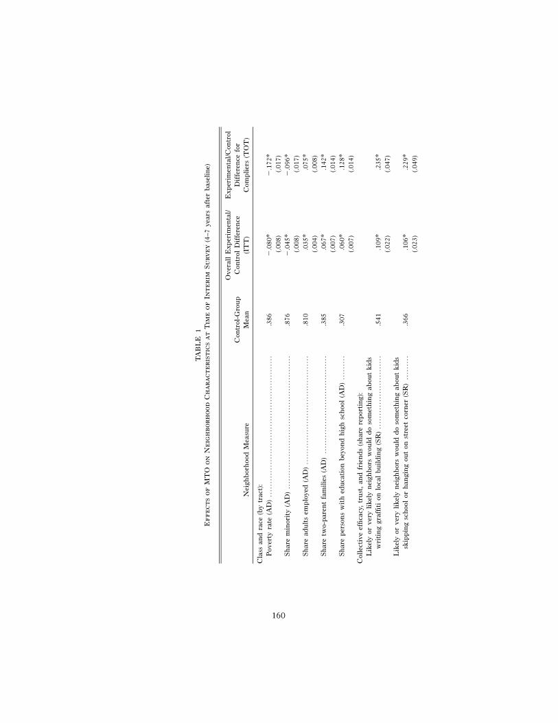
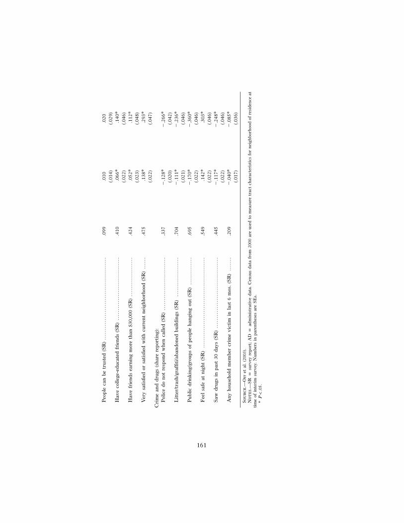
We believe that a more informative way to examine how MTO changesdiverse dimensions of neighborhood environments for participating fam-ilies is to calculate ITT and TOT impacts on continuous measures ofneighborhood characteristics. The results shown in table 1 demonstratethat, despite the fact that only 47% of experimental-group families movedthrough MTO, and some then moved back on their own to somewhathigher-poverty areas over time, very large changes in a wide range ofneighborhood attributes persisted at the time the interim MTO surveyswere conducted. For example, the TOT impact reported in the first rowof table 1 shows that at the time of the interim survey, the average complierin the experimental group lived in a census tract with a poverty rate about17 percentage points below that of the control group (about 45% of thecontrol-group mean).13 The TOT effect on tract share minority is smaller(by 9.6 percentage points, or about 11% of the control mean). But thereare large TOT effects on other tract sociodemographic attributes, includ-ing the share of two-parent families (14 percentage points, or about 37%of the control mean) and the share of tract adults who have more thana high school education (13 percentage points, or about 42% of the controlmean).
We also see large MTO effects on the types of neighborhood socialprocesses or institutions that sociologists often emphasize as the key be-havioral mechanisms behind neighborhood effects on behavior. For ex-ample, experimental-group compliers are about 27 percentage points lesslikely than controls to report that the police do not respond to 911 calls
12 Using the data on addresses six years after baseline that are available for aroundtwo-thirds of the MTO sample, we see only 9% of MTO experimental compliers livingin tracts with poverty rates of 40% or more, compared to 43% of the control group.If we use a lower threshold for “high-poverty tracts” of 30% poverty rate or more,four years after random assignment we see 16% of MTO experimental compliers livingin tracts with poverty rates of 30% or more, compared to 73% of the control group.Six years after random assignment, about 20% of the experimental compliers are intracts with poverty rates of 30% or more, compared to 64% of the control group.13 The most appropriate benchmark for the TOT estimate is actually the averageoutcome among those families assigned to the control group who would have movedhad they been assigned to the treatment group, or the “control complier mean” (CCM);see Katz et al. 2001. However, in practice the CCM is usually fairly close to the overallcontrol mean, and so for simplicity we focus here on the latter.
160
TA
BL
E1
Ef
fect
so
fM
TO
on
Ne
igh
borh
ood
Ch
arac
teri
stic
sa
tT
ime
of
Int
erim
Su
rvey
(4–7
year
saf
ter
bas
elin
e)
Nei
ghbo
rhoo
dM
easu
reC
ontr
ol-G
rou
pM
ean
Ov
eral
lE
xper
imen
tal/
Con
trol
Dif
fere
nce
(IT
T)
Exp
erim
enta
l/Con
trol
Dif
fere
nce
for
Com
plie
rs(T
OT
)
Cla
ssan
dra
ce(b
ytr
act)
:P
over
tyra
te(A
D)
....
....
....
....
....
....
....
....
....
....
....
....
....
.386
�.0
80*
�.1
72*
(.008
)(.0
17)
Sh
are
min
orit
y(A
D)
....
....
....
....
....
....
....
....
....
....
....
....
..8
76�
.045
*�
.096
*(.0
08)
(.017
)S
har
ead
ults
emp
loye
d(A
D)
....
....
....
....
....
....
....
....
....
....
.810
.035
*.0
75*
(.004
)(.0
08)
Sh
are
two-
pare
nt
fam
ilie
s(A
D)
....
....
....
....
....
....
....
....
....
.385
.067
*.1
42*
(.007
)(.0
14)
Sh
are
per
son
sw
ith
educ
atio
nb
eyon
dh
igh
sch
ool
(AD
)..
....
...
.307
.060
*.1
28*
(.007
)(.0
14)
Col
lect
ive
effi
cacy
,tr
ust,
and
frie
nds
(sh
are
rep
orti
ng):
Lik
ely
orv
ery
like
lyn
eigh
bors
wou
ldd
oso
met
hin
gab
out
kid
sw
riti
ng
graf
fiti
onlo
cal
bui
ldin
g(S
R)
....
....
....
....
....
....
...
.541
.109
*.2
35*
(.022
)(.0
47)
Lik
ely
orv
ery
like
lyn
eigh
bors
wou
ldd
oso
met
hin
gab
out
kid
ssk
ipp
ing
sch
ool
orh
angi
ng
out
onst
reet
corn
er(S
R)
....
....
..3
66.1
06*
.229
*(.0
23)
(.049
)
161
Peo
ple
can
be
tru
sted
(SR
)..
....
....
....
....
....
....
....
....
....
....
.099
.010
.020
(.014
)(.0
29)
Hav
eco
lleg
e-ed
ucat
edfr
ien
ds(S
R)
....
....
....
....
....
....
....
....
.410
.066
*.1
40*
(.022
)(.0
46)
Hav
efr
ien
dsea
rnin
gm
ore
than
$30,
000
(SR
)..
....
....
....
....
...4
24.0
52*
.112
*(.0
23)
(.048
)V
ery
sati
sfied
orsa
tisfi
edw
ith
curr
ent
nei
ghbo
rhoo
d(S
R)
....
...4
75.1
38*
.293
*(.0
22)
(.047
)C
rim
ean
dd
rugs
(sh
are
rep
orti
ng):
Pol
ice
do
not
resp
ond
wh
enca
lled
(SR
)..
....
....
....
....
....
....
..3
37�
.128
*�
.266
*(.0
20)
(.042
)L
itte
r/tr
ash
/gra
ffiti
/ab
ando
ned
bui
ldin
gs(S
R)
....
....
....
....
....
.704
�.1
11*
�.2
36*
(.021
)(.0
46)
Pu
blic
dri
nk
ing/
grou
ps
ofp
eop
leh
angi
ng
out
(SR
)..
....
....
....
.695
�.1
70*
�.3
60*
(.022
)(.0
46)
Fee
lsa
feat
nig
ht
(SR
)..
....
....
....
....
....
....
....
....
....
....
....
.549
.142
*.3
03*
(.022
)(.0
46)
Saw
dru
gsin
pas
t30
day
s(S
R)
....
....
....
....
....
....
....
....
....
.445
�.1
17*
�.2
48*
(.022
)(.0
46)
An
yh
ouse
hol
dm
emb
ercr
ime
vic
tim
inla
st6
mos
.(S
R)
....
...
.209
�.0
40*
�.0
85*
(.017
)(.0
36)
So
urc
e.—
Orr
etal
.(2
003)
.N
ot
es.
—S
Rp
surv
eyre
por
t;A
Dp
adm
inis
trat
ive
dat
a.C
ensu
sd
ata
from
2000
are
use
dto
mea
sure
trac
tch
arac
teri
stic
sfo
rn
eigh
bor
hoo
dof
resi
denc
eat
tim
eof
inte
rim
surv
ey.
Nu
mbe
rsin
par
enth
eses
are
SE
s.*
.P
!.0
5
American Journal of Sociology
162
for service, which is nearly 80% of the control-group mean. Experimentalcompliers are much less likely than controls to report that their neigh-borhoods are plagued by social disorder, as indicated by litter, graffiti,public drinking, or groups hanging out at night in public spaces. Exper-imental-group compliers are in turn much more likely than controls toindicate that they feel safe at night in their neighborhood (by 30 percentagepoints, about 55% of the control mean) and are less likely to indicate thatanyone in the household was victimized by a crime in the past six months(by nearly 9 percentage points, or about two-fifths of the control mean).Informal social control seems to be more common in the neighborhoodsin which the experimental-group families reside four to seven years afterrandom assignment. Although experimental adults are not more likelythan controls to report that they think, in general, that people can betrusted (responses by both groups suggest low levels of trust), adults inthe experimental group are more likely to have college-educated friendsor friends who earn more than $30,000 per year.
Note again that we are measuring neighborhood characteristics in table1 at the time of the interim surveys (four to seven years after randomassignment) using either survey reports or data from the 2000 census.Because some of the neighborhoods experimental-group families movedinto were deteriorating from 1990 to 2000, and some MTO families movedagain on their own, MTO’s impacts on the average neighborhood envi-ronment families experienced from baseline to the time of these surveysare even larger than table 1 would suggest.
It is hard to think of any larger randomized social policy interventionthan MTO. MTO families were assisted in moving from some of the mostviolent and distressed housing projects in America. This was not a pro-gram that simply offered short-term job training, like the Job TrainingPartnership Act (JTPA) programs (Bloom et al. 1996; Orr et al. 1996);changed health insurance co-payment rates, like the RAND health ex-periment (Newhouse and IEG 1993); or helped with interview skills, likethe job-search assistance experiments. The living arrangements for peoplewho moved through MTO were fundamentally transformed for years.
The Role of Neighborhood Racial Integration
While CM acknowledge that MTO helped experimental-group compliersmove to neighborhoods that were less disadvantaged and dangerous alongmany dimensions, they argue that MTO provides a weak test of neigh-borhood effects because of its relatively limited impact on racial integra-tion. “MTO shuffled families around within the confines of racially seg-regated neighborhoods, exposing them to a limited range of resources andopportunities” (pp. 137–38) and so “stacked the deck against finding neigh-
MTO Symposium: What Can We Learn from MTO?
163
borhood effects” (p. 116). Even MTO experimental-group compliers con-tinued to live in census tracts that were lower poverty but still heavilyminority.
But the argument that mobility programs that achieve social class in-tegration must also necessarily achieve racial integration in order tochange behavior would appear to be inconsistent with the influentialtheoretical model developed by Wilson (1987). The precipitating event inthe Wilson model is the flight of black working- and middle-class familiesduring the 1960s and 1970s, a “profound social transformation” that con-tributed to high prevalence rates among the remaining families of crime,out-of-wedlock births, female-headed families, and welfare dependency(Wilson 1987, p. 49). In Wilson’s model, the exodus of middle- and work-ing-class families was particularly important because these families servedas “a social buffer,” as “mainstream role models that help keep alive theperception that education is meaningful, that steady employment is aviable alternative to welfare, and that family stability is the norm, notthe exception” (Wilson 1987, p. 49). MTO as implemented would seemto provide an almost perfect test of this theory—it helped families moveout of some of the most unsafe neighborhoods in America into neigh-borhoods with substantial shares of middle-class minority residents whocould potentially serve as role models.
CM’s argument that large changes in both neighborhood racial com-position and social class composition are necessary to change behavior isalso inconsistent with our findings of MTO impacts on a number of keyoutcomes besides economic self-sufficiency. For example, adults assignedto the MTO experimental rather than the control group reported largeimprovements in mental health; the ITT impact on Kessler’s K-6 indexof psychological distress (which is the fraction of six questions aboutpsychological distress that the respondent answered in the affirmative) isequal to around �0.1 standard deviations, with a TOT impact of �0.2standard deviations—about the same magnitude change in mental healthoutcomes as results from current best-practice antidepressant drug treat-ment (Kling et al. 2007, pp. 92, 102). The MTO impact on the K-6 mentalhealth index for young females is even larger, with ITT and TOT esti-mates equal to �0.29 and �0.59 standard deviations, respectively. Duringthe first few years after random assignment, MTO reduced the numberof arrests of young females by nearly half and even for young malesreduced the number of arrests for violent crimes by more than one-third(Kling et al. 2005, p. 104).
It is true that after a few years, young males assigned to the experi-mental group wind up with worse outcomes than those assigned to the
American Journal of Sociology
164
control group.14 For policy purposes, we would hope for positive effectsrather than these large adverse effects on many outcomes for young males.But the fact that even the adverse responses of some young males to MTOare so large seems inconsistent with the characterization of MTO as a“weak intervention.”15
Additional evidence against CM’s claim that racial integration is anecessary condition for changing economic outcomes comes from theirown estimates. For example, estimates presented in their table 5 indicatethat each additional month spent in a low-poverty integrated neighbor-hood increases employment rates by 1.1 percentage points, and each extramonth spent in a low-poverty segregated neighborhood increases em-ployment rates by 1.1 percentage points. This is not a very large difference.The estimated effects in CM’s study of spending more time in a low-poverty integrated neighborhood versus a low-poverty segregated neigh-borhood are also quite similar for weekly earnings (1.89 vs. 1.53; SE p0.91 and 0.81, respectively), use of TANF (Temporary Assistance forNeedy Families) (�0.009 vs. �0.008; SE p 0.006 and 0.005), and foodstamp use (�0.015 vs. �0.014; SE p 0.005 and 0.004). Moreover, as wedemonstrate below, CM’s estimates of the effects of time spent in low-poverty integrated areas are sensitive to their specific modeling and es-timation decisions.
CM suggest that corroborating evidence for the importance of inte-grating by race as well as by social class in order to influence adulteconomic outcomes can be found in the Chicago Gautreaux program,which placed families in neighborhoods on the basis of race rather thanclass. Rosenbaum (1995) reports that around 64% of adults who movedto the suburbs through Gautreaux were employed at the time of a 1988survey (around five to six years after initial Gautreaux placements), com-pared with about 51% of city movers. But the difference in results betweenMTO and Gautreaux could also be explained by potential selection prob-lems with evaluations of the Gautreaux program.
14 For instance, administrative arrest histories show that, three to four years afterrandom assignment, the experimental ITT impact on property crime arrests is equalto 0.038 more arrests per male youth per year, nearly half the control mean (Kling etal. 2005, p. 104). The MTO interim survey data, collected on average about five yearsafter random assignment, show an experimental ITT impact on the share of youngmales reporting a nonsports accident or injury in the past year of 9 percentage points(about 150% of the control mean), while the experimental ITT impact on smoking inthe past 30 days is 10 percentage points, over 80% of the control mean (Kling et al.2007, p. 92).15 It is also true that MTO wound up generating relatively modest changes in accessto jobs (Kling et al. 2007). While this mechanism is central to “spatial mismatch”theories (Kain 1968), it is not central to many of the key theories emphasized bysociologists as to why neighborhoods might affect economic outcomes.
MTO Symposium: What Can We Learn from MTO?
165
Gautreaux was not a randomized experiment in which some familiesreceived the Gautreaux offer and others did not. Families in Gautreauxwere offered rental units by the nonprofit agency running the programin the order in which they were assigned to the waiting list. A commonclaim is that Gautreaux families accepted the first or second rental unitoffered to them by the local nonprofit agency, but documentation of thisoffer-and-accept process is not available, and so there remains some ques-tion about the possibility of selection into suburban rather than urbanneighborhoods. Rosenbaum’s (1995) results for effects on adult labor mar-ket outcomes, based on comparisons between suburban and city movers,are drawn from a follow-up survey of Gautreaux movers with a responserate of 59%. Mendenhall, DeLuca, and Duncan (2006) use administrativedata on Gautreaux families to overcome problems of selective surveysample attrition and find no detectable differences in economic outcomesbetween city and suburban movers, although they do find signs of rela-tively small associations between some specific socioeconomic or racialneighborhood characteristics and economic outcomes. But all of theseresults are difficult to interpret, given evidence of an association betweenplacement neighborhoods and baseline family and origin-neighborhoodattributes.16
In sum, it may be true that residential integration by race is particularlyimportant for some behavioral outcomes, including violent behavior (Lud-wig and Kling 2007). But there is not a very strong empirical basis atpresent for suggesting that a large change in neighborhood racial com-position is a necessary condition for affecting behavioral outcomes. Tothe contrary, there is strong evidence from our own experimental analysisof MTO that the intervention was in fact powerful enough to yield largechanges in a number of key outcomes aside from adult economic self-sufficiency.
WHAT CAN WE LEARN FROM CM’S NEW ESTIMATES?
We have argued above that CM are wrong in claiming that our previousexperimental ITT and TOT estimates from the MTO data are uninform-ative about the existence of neighborhood effects. Nevertheless, we aresympathetic to CM’s goal of trying to learn more about who benefits the
16 Mendenhall et al. (2006) find that, compared to suburban movers, city movers inGautreaux have slightly older children (measured by age of youngest child), are morelikely to live in public housing at baseline, and generally come from more disadvan-taged and dangerous baseline neighborhoods. Votruba and Kling (2004) also find evi-dence for an association between baseline characteristics and placement neighborhoodoutcomes.
American Journal of Sociology
166
most from MTO and why, and so in this section we consider the questionof how much useful information their nonexperimental estimates con-tribute to our understanding of neighborhood effects. Unfortunately, ourconclusion is that they do not contribute much. The most important reasonis that their nonexperimental cross-section regression estimates are likelyto be affected by selection bias. Another reason is that their research designconfounds treatment effect differences by random assignment cohort withdifferences in time spent in low-poverty neighborhoods. We also dem-onstrate that even if we ignore these two significant problems, their find-ings that adult labor market outcomes are improved by additional timespent in low-poverty integrated neighborhoods appears to be sensitive totheir specific modeling and estimation decisions.
Replicating CM’s Estimates
We begin by replicating CM’s estimates using their model specificationand version of the MTO data set, which they generously shared with us.Before presenting these results, we first briefly review their estimationframework. CM’s main estimates for neighborhood “associations” areshown in their tables 5 and 6. The key explanatory variables are measuresof months of exposure to low-poverty integrated, low-poverty segregated,and poor neighborhoods. They also control for indicators for assignmentgroup and compliance status (i.e., variables indicating experimental non-compliers and experimental compliers), as well as a standard set of base-line characteristics that we have used in our own previous research, in-cluding the adult’s own sociodemographic characteristics and baselineemployment status.
As shown in the top row of table 2, we are able to reproduce theirpoint estimates and standard errors almost exactly for three of the fouroutcomes they examine: employed at the time of the MTO interim survey,TANF receipt, and food stamp receipt. Our estimates differ from theirsfor weekly earnings because we estimate models for all four outcomesusing sampling weights that adjust for the fact that there was a changeduring the course of the MTO study period in the probability that enrolleeswould be assigned to each of the three mobility groups in the demon-stration. CM use these sampling weights for their estimates for employ-ment, TANF receipt, and food stamp receipt, but they estimate weeklyearnings without weights.17 We follow CM’s convention of showing actuallogit or Tobit coefficients and standard errors, although our own pref-erence would have been to show the results in a way that makes it easier
17 When we estimate the model without weights, we can replicate their unweightedestimates exactly.
MTO Symposium: What Can We Learn from MTO?
167
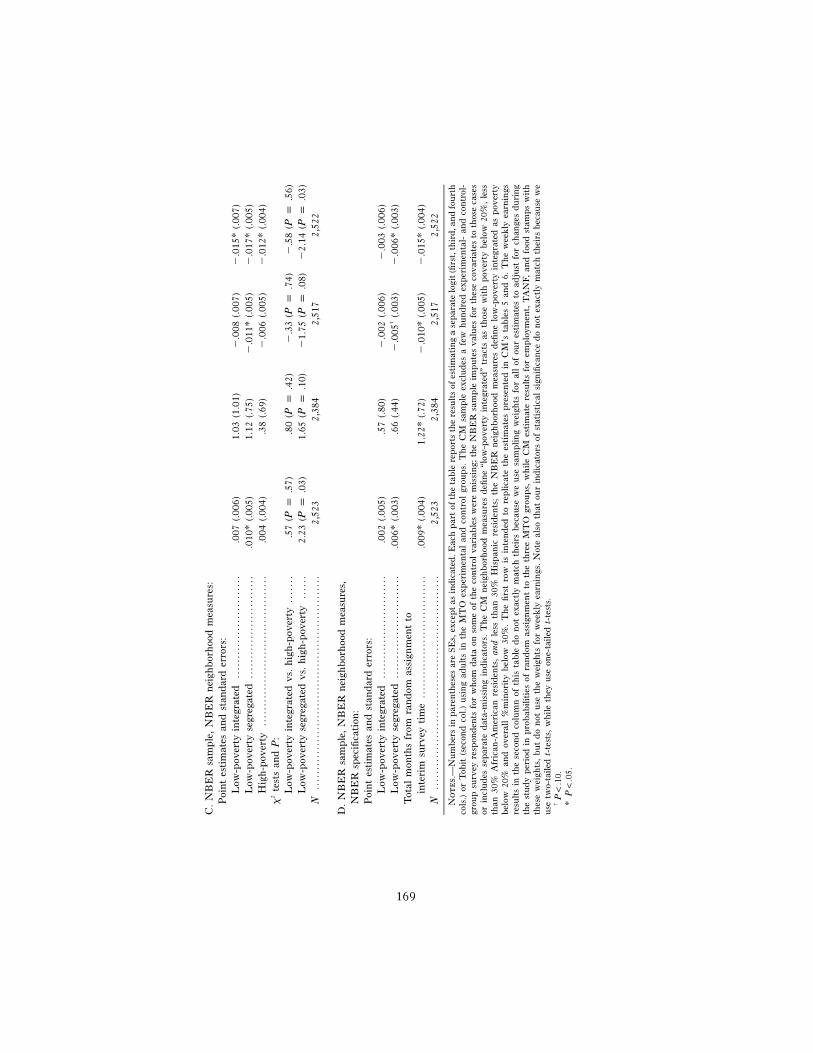
to understand the magnitude of the estimated effects—for example, forthe dichotomous dependent variables we would have shown either oddsratios or, better still, average marginal effects.18
Note that our indications of statistical significance do not quite matchtheirs (e.g., with TANF receipt), because CM are calculating P valuesusing one-tailed t-tests. We instead use P values calculated from two-tailed t-tests, since much of the theoretical work in this area suggests thepossibility of adverse effects of MTO moves on behavioral outcomes(Jencks and Mayer 1990; Luttmer 2005). The fact that assignment to theMTO experimental rather than the control group has, on balance, det-rimental effects for young males by the time of the interim survey wouldseem to justify this decision.
A different concern with CM’s statistical tests is that they seem to beusing the wrong null hypothesis for testing whether there are neighbor-hood effects on economic outcomes. By neighborhood effect, we usuallymean that time spent in a less disadvantaged neighborhood has morebeneficial impacts on behavioral outcomes of interest than does time spentin a relatively more disadvantaged neighborhood. CM’s claim for anassociation between low-poverty neighborhoods and economic outcomesis derived from testing whether the estimated coefficients for the effectsof months in a low-poverty integrated or segregated census tract are dif-ferent from zero. But given that the counterfactual of interest here is timespent in a high-poverty rather than low-poverty area, we should be testingwhether the coefficients for time in low-poverty integrated or segregatedtracts are different from the coefficient for time in high-poverty tracts.We present the result of these tests in part A of table 2; we find that atthe usual 5% cutoff we cannot reject the hypothesis that the effects ofliving in low-poverty integrated neighborhoods are the same as those ofliving in high-poverty neighborhoods. Extra exposure to low-poverty seg-regated areas boosts employment rates and reduces food stamp receipt,but it has no significant effect on earnings or TANF receipt.
During the course of working with CM’s data, we realized that theyhandle missing values among the MTO baseline control variables in adifferent way from our own team’s standard practice when analyzingMTO data. Specifically, for families missing values for any baseline controlvariables, we either impute values or include missing-data indicators for
18 Most software packages calculate marginal effects (dp/dx) at the mean values of thecontrol variables. This can be problematic in cases such as MTO, where many of ourright-hand-side variables are dichotomous, and so no one in the MTO sample is atthe means. We instead calculate the marginal effects for everyone in the MTO sampleand then take the average of these marginal effects (see Chamberlain [1984, p. 1274]for a conceptual discussion; for calculating the average marginal effects in Stata, seeBartus [2005]).

168
TA
BL
E2
Re
plic
atin
ga
nd
Ex
ten
din
gC
M’s
Est
imat
esf
orE
ffe
cts
of
Tim
ein
Low
-a
nd
Hig
h-P
over
tyT
rac
tso
nE
con
omic
Ou
tcom
es
Em
plo
yed
Wee
kly
Ear
nin
gsT
AN
FR
ecei
ptF
ood
Sta
mp
Rec
eipt
A.
CM
sam
ple
,C
Mn
eigh
borh
ood
mea
sure
s:P
oint
esti
mat
esan
dst
anda
rder
rors
:L
ow-p
over
tyin
tegr
ated
....
....
....
....
....
....
...0
11†
(.006
)1.
47(.9
1)�
.009
(.006
)�
.015
*(.0
06)
Low
-pov
erty
segr
egat
ed..
....
....
....
....
....
....
.011
*(.0
05)
.94
(.81)
�.0
08(.0
06)
�.0
14*
(.005
)H
igh
-pov
erty
....
....
....
....
....
....
....
....
....
...0
05(.0
04)
.32
(.73)
�.0
03(.0
05)
�.0
09*
(.004
)x
2te
sts
and
P:
Low
-pov
erty
inte
grat
edv
s.h
igh
-pov
erty
....
...
1.42
(Pp
.15)
1.80
(Pp
.07)
�1.
12(P
p.2
6)�
1.55
(Pp
.12)
Low
-pov
erty
segr
egat
edv
s.h
igh
-pov
erty
....
..2.
04(P
p.0
4)1.
30(P
p.2
0)�
1.45
(Pp
.15)
�2.
08(P
p.0
4)N
....
....
....
....
....
....
....
....
....
....
....
....
....
..2,
293
2,16
62,
287
2,29
2
B.
NB
ER
sam
ple
,C
Mn
eigh
borh
ood
mea
sure
s:P
oint
esti
mat
esan
dst
anda
rder
rors
:L
ow-p
over
tyin
tegr
ated
....
....
....
....
....
....
...0
09†
(.005
)1.
28(.8
7)�
.011
†(.0
06)
�.0
18*
(.006
)L
ow-p
over
tyse
greg
ated
....
....
....
....
....
....
...0
10*
(.005
)1.
04(.7
7)�
.010
*(.0
05)
�.0
16*
(.005
)H
igh
-pov
erty
....
....
....
....
....
....
....
....
....
...0
04(.0
04)
.38
(.69)
�.0
06(.0
05)
�.0
11*
(.004
)x
2te
sts
and
P:
Low
-pov
erty
inte
grat
edv
s.h
igh
-pov
erty
....
...
1.27
(Pp
.21)
1.46
(Pp
.14)
�1.
35(P
p.1
8)�
1.65
(Pp
.10)
Low
-pov
erty
segr
egat
edv
s.h
igh
-pov
erty
....
..2.
08(P
p.0
4)1.
40(P
p.1
6)�
1.46
(Pp
.14)
�1.
79(P
p.0
7)N
....
....
....
....
....
....
....
....
....
....
....
....
....
..2,
523
2,38
42,
517
2,52
2
169
C.
NB
ER
sam
ple
,N
BE
Rn
eigh
borh
ood
mea
sure
s:P
oint
esti
mat
esan
dst
anda
rder
rors
:L
ow-p
over
tyin
tegr
ated
....
....
....
....
....
....
...0
07(.0
06)
1.03
(1.0
1)�
.008
(.007
)�
.015
*(.0
07)
Low
-pov
erty
segr
egat
ed..
....
....
....
....
....
....
.010
*(.0
05)
1.12
(.75)
�.0
11*
(.005
)�
.017
*(.0
05)
Hig
h-p
over
ty..
....
....
....
....
....
....
....
....
....
.004
(.004
).3
8(.6
9)�
.006
(.005
)�
.012
*(.0
04)
x2
test
san
dP
:L
ow-p
over
tyin
tegr
ated
vs.
hig
h-p
over
ty..
....
..5
7(P
p.5
7).8
0(P
p.4
2)�
.33
(Pp
.74)
�.5
8(P
p.5
6)L
ow-p
over
tyse
greg
ated
vs.
hig
h-p
over
ty..
....
2.23
(Pp
.03)
1.65
(Pp
.10)
�1.
75(P
p.0
8)�
2.14
(Pp
.03)
N..
....
....
....
....
....
....
....
....
....
....
....
....
....
2,52
32,
384
2,51
72,
522
D.
NB
ER
sam
ple
,N
BE
Rn
eigh
borh
ood
mea
sure
s,N
BE
Rsp
ecifi
cati
on:
Poi
ntes
tim
ates
and
stan
dard
erro
rs:
Low
-pov
erty
inte
grat
ed..
....
....
....
....
....
....
.002
(.005
).5
7(.8
0)�
.002
(.006
)�
.003
(.006
)L
ow-p
over
tyse
greg
ated
....
....
....
....
....
....
...0
06*
(.003
).6
6(.4
4)�
.005
†(.0
03)
�.0
06*
(.003
)T
otal
mon
ths
from
ran
dom
assi
gnm
ent
toin
teri
msu
rvey
tim
e..
....
....
....
....
....
....
....
..0
09*
(.004
)1.
22*
(.72)
�.0
10*
(.005
)�
.015
*(.0
04)
N..
....
....
....
....
....
....
....
....
....
....
....
....
....
2,52
32,
384
2,51
72,
522
No
te
s.—
Nu
mb
ers
inp
aren
thes
esar
eS
Es,
exce
pt
asin
dic
ated
.Eac
hp
art
ofth
eta
ble
rep
orts
the
resu
lts
ofes
tim
atin
ga
sep
arat
elo
git
(firs
t,th
ird
,an
dfo
urt
hco
ls.)
orT
obit
(sec
ond
col.)
usi
ng
adu
lts
inth
eM
TO
exp
erim
enta
lan
dco
ntr
olgr
oup
s.T
he
CM
sam
ple
excl
ud
esa
few
hu
nd
red
exp
erim
enta
l-an
dco
ntr
ol-
grou
psu
rvey
resp
ond
ents
for
wh
omd
ata
onso
me
ofth
eco
ntr
olv
aria
ble
sw
ere
mis
sin
g;th
eN
BE
Rsa
mp
leim
pu
tes
val
ues
for
thes
eco
var
iate
sto
thos
eca
ses
orin
clu
des
sep
arat
ed
ata-
mis
sin
gin
dic
ator
s.T
he
CM
nei
ghb
orh
ood
mea
sure
sd
efin
e“l
ow-p
over
tyin
tegr
ated
”tr
acts
asth
ose
wit
hp
over
tyb
elow
20%
,le
ssth
an30
%A
fric
an-A
mer
ican
resi
den
ts,
and
less
than
30%
His
pan
icre
sid
ents
;th
eN
BE
Rn
eigh
bor
hoo
dm
easu
res
defi
ne
low
-pov
erty
inte
grat
edas
pov
erty
bel
ow20
%an
dov
eral
l%
min
orit
yb
elow
30%
.T
he
firs
tro
wis
inte
nd
edto
rep
lica
teth
ees
tim
ates
pre
sen
ted
inC
M’s
tab
les
5an
d6.
Th
ew
eek
lyea
rnin
gsre
sult
sin
the
seco
nd
colu
mn
ofth
ista
ble
do
not
exac
tly
mat
chth
eirs
bec
ause
we
use
sam
pli
ng
wei
ghts
for
all
ofou
res
tim
ates
toad
just
for
chan
ges
du
ring
the
stu
dy
per
iod
inp
rob
abil
itie
sof
ran
dom
assi
gnm
ent
toth
eth
ree
MT
Ogr
oup
s,w
hil
eC
Mes
tim
ate
resu
lts
for
emp
loym
ent,
TA
NF,
and
food
stam
psw
ith
thes
ew
eigh
ts,
bu
td
on
otu
seth
ew
eigh
tsfo
rw
eek
lyea
rnin
gs.
Not
eal
soth
atou
rin
dic
ator
sof
stat
isti
cal
sign
ifica
nce
do
not
exac
tly
mat
chth
eirs
bec
ause
we
use
two-
taile
dt-
test
s,w
hile
they
use
one-
taile
dt-
test
s.†
.P
!.1
0*
.P
!.0
5

American Journal of Sociology
170
each control variable (equal to 1 in cases where the variable’s value wasmissing, 0 otherwise). CM instead code many of these cases as missing.In part B of table 2, we show that using imputed values for these controlvariables increases the sample size by a few hundred cases but has littleeffect on the qualitative pattern revealed by the data.
Working with CM’s data, we also discovered that their system forclassifying low-poverty integrated versus segregated neighborhoods is dif-ferent from what we had inferred from their article. Specifically, they say,“Following the criteria used by Gautreaux, we classify census tracts thatare under 30% minority (black and Hispanic) as ‘integrated neighbor-hoods’ and those whose minority percentage exceeds this level as ‘seg-regated.’” (p. 117). The Gautreaux program’s criterion was to move fam-ilies into “predominantly white” tracts with less than 30%African-American families (Keels et al. 2005). What CM did was to classifylow-poverty tracts as integrated if the census tract had less than 30%African-American residents and less than 30% Hispanic residents—so thatin principle, a census tract that was nearly 60% minority would still becounted as integrated so long as the African-American and Hispanicshares were still both individually below 30%.
In part C of table 2, we show what happens when we use an equallydefensible measure of what constitutes an integrated neighborhood—spe-cifically, census tracts that are less than 30% minority overall (African-American, Hispanic, and other minority groups together). This definitionhas the virtue of being more consistent with the Gautreaux program’sgoals of moving families to “predominantly white” neighborhoods. Com-pared to CM’s classification system, this definition reduces the amountof time that MTO experimental-group families spent in low-poverty in-tegrated neighborhoods.19 When we use our system to define integratedneighborhoods as less than 30% minority, rather than less than 30% blackand less than 30% Hispanic, we do not find any evidence that extra timein low-poverty integrated tracts rather than high-poverty tracts improvesany of the economic outcomes CM consider. There do still appear to besigns of some effect of extra time in low-poverty segregated areas, contraryto CM’s hypothesis that race and social class integration together arenecessary to improve adult economic outcomes. More generally, if wererun this model using a measure of total months spent in low-povertycensus tracts (regardless of whether they are integrated or segregated), wedo not find any evidence that living in a low-poverty rather than high-
19 CM’s system suggests that experimental families overall spent about 8.1 months inlow-poverty integrated neighborhoods, while our definition suggests something closerto 3.8 months. Under our definition, experimental families spent somewhat moremonths in low-poverty segregated tracts compared to CM’s system (21.39 vs. 17.08).
MTO Symposium: What Can We Learn from MTO?
171
poverty area affects the economic outcomes studied by CM. In any case,even these estimates are overstated, because they confound cohort withtime effects.
Cohort Effects vs. the Effects of Time in Low-Poverty Areas
One source of bias in CM’s estimates is that they confound the effectson economic outcomes of spending more time in a low-poverty area withdifferences in program impacts that vary by randomization entry cohortsin MTO. Because of the limited capacity of the nonprofit agencies thathelped MTO experimental families relocate, and for other reasons, familieswho enrolled in MTO were randomly assigned into different mobilitygroups over an extended period of time ranging from 1994 to 1998. CM’skey explanatory variables of interest are the number of months spent inlow-poverty and high-poverty areas, both of which will(! 20%) (≥ 20%)on average be higher for earlier cohorts for mechanical reasons. In fact,the only reason CM are even able to estimate a model that controls fortime in both low-poverty and high-poverty census tracts, yet avoids theproblem of perfect multicollinearity, is that some families were randomlyassigned earlier in time than others and so will have more months ofaddress data available between the time of randomization and the interimMTO survey.20 CM’s estimates confound cohort differences in MTO im-pacts on survey outcomes with changes in impacts over time for reasonssimilar to those in demography that often make it hard to disentangleage, period, and cohort effects.
Some evidence for cohort differences in MTO impacts comes from table3, taken from Orr et al. (2003, table G-7), which shows TOT impacts onadministrative data measures for TANF and food stamp benefits, takenfive years after random assignment for cohorts randomly assigned earlier(with an average time between randomization and interim survey of 81
20 If all MTO families had the same amount of postrandomization data (the samenumber of months between time of random assignment and time at which the interimMTO survey was conducted), the explanatory variables for number of months in low-poverty integrated, low-poverty segregated, and high-poverty census tracts would beperfectly multicollinear. This is easy to see by imagining that we simply rescaled thevariables for time in low-poverty and high-poverty areas by dividing by the samplemean for total number of months of post–random assignment address data. If theamount of postrandomization data were the same for everyone (always equal to themean), then the measures for share time in low-poverty and high-poverty areas wouldtogether sum to one.
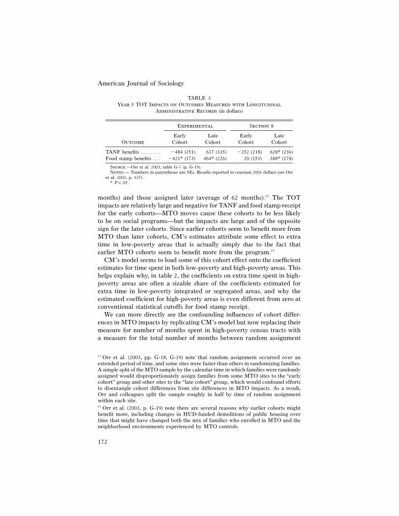
American Journal of Sociology
172
TABLE 3Year 5 TOT Impacts on Outcomes Measured with Longitudinal
Administrative Records (in dollars)
Outcome
Experimental Section 8
EarlyCohort
LateCohort
EarlyCohort
LateCohort
TANF benefits . . . . . . . . . . �484 (251) 617 (335) �252 (218) 628* (236)Food stamp benefits . . . . �421* (173) 464* (226) 20 (153) 388* (178)
Source.—Orr et al. 2003, table G-7 (p. G-19).Notes.— Numbers in parentheses are SEs. Results reported in constant 2001 dollars (see Orr
et al. 2003, p. 137).* .P ! .05
months) and those assigned later (average of 62 months).21 The TOTimpacts are relatively large and negative for TANF and food stamp receiptfor the early cohorts—MTO moves cause these cohorts to be less likelyto be on social programs—but the impacts are large and of the oppositesign for the later cohorts. Since earlier cohorts seem to benefit more fromMTO than later cohorts, CM’s estimates attribute some effect to extratime in low-poverty areas that is actually simply due to the fact thatearlier MTO cohorts seem to benefit more from the program.22
CM’s model seems to load some of this cohort effect onto the coefficientestimates for time spent in both low-poverty and high-poverty areas. Thishelps explain why, in table 2, the coefficients on extra time spent in high-poverty areas are often a sizable share of the coefficients estimated forextra time in low-poverty integrated or segregated areas, and why theestimated coefficient for high-poverty areas is even different from zero atconventional statistical cutoffs for food stamp receipt.
We can more directly see the confounding influences of cohort differ-ences in MTO impacts by replicating CM’s model but now replacing theirmeasure for number of months spent in high-poverty census tracts witha measure for the total number of months between random assignment
21 Orr et al. (2003, pp. G-18, G-19) note that random assignment occurred over anextended period of time, and some sites were faster than others in randomizing families.A simple split of the MTO sample by the calendar time in which families were randomlyassigned would disproportionately assign families from some MTO sites to the “earlycohort” group and other sites to the “late cohort” group, which would confound effortsto disentangle cohort differences from site differences in MTO impacts. As a result,Orr and colleagues split the sample roughly in half by time of random assignmentwithin each site.22 Orr et al. (2003, p. G-19) note there are several reasons why earlier cohorts mightbenefit more, including changes in HUD-funded demolitions of public housing overtime that might have changed both the mix of families who enrolled in MTO and theneighborhood environments experienced by MTO controls.
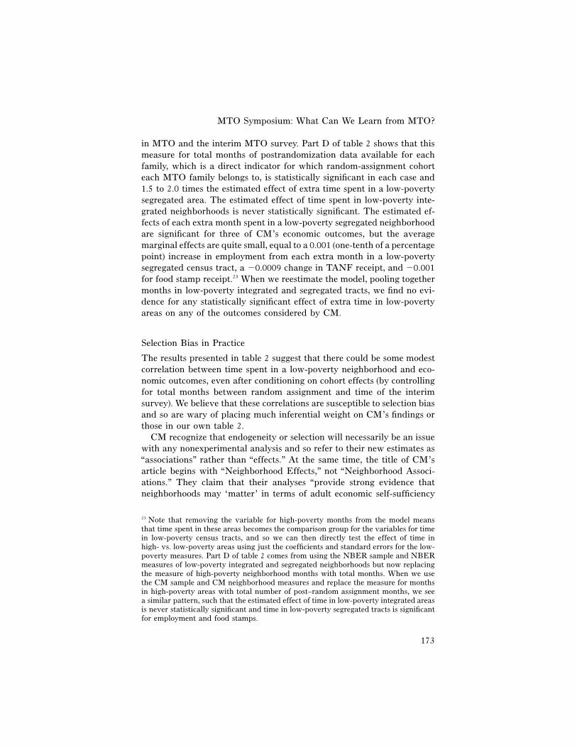
MTO Symposium: What Can We Learn from MTO?
173
in MTO and the interim MTO survey. Part D of table 2 shows that thismeasure for total months of postrandomization data available for eachfamily, which is a direct indicator for which random-assignment cohorteach MTO family belongs to, is statistically significant in each case and1.5 to 2.0 times the estimated effect of extra time spent in a low-povertysegregated area. The estimated effect of time spent in low-poverty inte-grated neighborhoods is never statistically significant. The estimated ef-fects of each extra month spent in a low-poverty segregated neighborhoodare significant for three of CM’s economic outcomes, but the averagemarginal effects are quite small, equal to a 0.001 (one-tenth of a percentagepoint) increase in employment from each extra month in a low-povertysegregated census tract, a �0.0009 change in TANF receipt, and �0.001for food stamp receipt.23 When we reestimate the model, pooling togethermonths in low-poverty integrated and segregated tracts, we find no evi-dence for any statistically significant effect of extra time in low-povertyareas on any of the outcomes considered by CM.
Selection Bias in Practice
The results presented in table 2 suggest that there could be some modestcorrelation between time spent in a low-poverty neighborhood and eco-nomic outcomes, even after conditioning on cohort effects (by controllingfor total months between random assignment and time of the interimsurvey). We believe that these correlations are susceptible to selection biasand so are wary of placing much inferential weight on CM’s findings orthose in our own table 2.
CM recognize that endogeneity or selection will necessarily be an issuewith any nonexperimental analysis and so refer to their new estimates as“associations” rather than “effects.” At the same time, the title of CM’sarticle begins with “Neighborhood Effects,” not “Neighborhood Associ-ations.” They claim that their analyses “provide strong evidence thatneighborhoods may ‘matter’ in terms of adult economic self-sufficiency
23 Note that removing the variable for high-poverty months from the model meansthat time spent in these areas becomes the comparison group for the variables for timein low-poverty census tracts, and so we can then directly test the effect of time inhigh- vs. low-poverty areas using just the coefficients and standard errors for the low-poverty measures. Part D of table 2 comes from using the NBER sample and NBERmeasures of low-poverty integrated and segregated neighborhoods but now replacingthe measure of high-poverty neighborhood months with total months. When we usethe CM sample and CM neighborhood measures and replace the measure for monthsin high-poverty areas with total number of post–random assignment months, we seea similar pattern, such that the estimated effect of time in low-poverty integrated areasis never statistically significant and time in low-poverty segregated tracts is significantfor employment and food stamps.

American Journal of Sociology
174
as well, though having more specific neighborhood targets and a longerrequired stay than MTO did are important. Thus, there is substantialevidence for keeping geographically specific vouchers on the table in orderto offer low-income families a chance to improve their well-being” (pp.139–40).
CM are trying to thread a narrow rhetorical needle. They acknowledgethat their estimates may be susceptible to some degree of selection bias,and so they do not want to claim that their new findings capture theprecise causal effects of neighborhood environments on economic out-comes. But at the same time they want to argue that their new estimatesprovide enough useful information about neighborhood effects to informpolicy decisions. What they seem to be implicitly claiming is that theirestimates are, if not exactly right, at least in the right ballpark.
However, there is no way to tell whether these results are in fact in theright ballpark. Recall that CM’s model includes measures of time spentin low-poverty neighborhoods and indicators for MTO treatment groupand compliance status. CM’s estimates for the effects of specific neigh-borhood characteristics on economic outcomes are thus essentially aweighted average of three regression-adjusted differences: the mean out-comes for experimental-group compliers who chose (or were able) to spenda long time in low-poverty areas versus compliers who spent less time inlow-poverty areas; the difference in outcomes between experimental non-compliers who spent a long time in low-poverty areas versus those whospent less time in low-poverty areas; and the difference in outcomes be-tween control families who spent more time in low-poverty areas thanother families in the control group.
CM’s approach to estimating the effects of cumulative time spent inlow-poverty areas on employment outcomes measured from the interimsurvey is particularly vulnerable to selection biases. For example, anynumber of chance circumstances that might lead quickly to an unusuallygood job situation (e.g., seeing a “help wanted” sign for a well-paying jobin a neighborhood store) will increase the chances of being able to affordto continue to live in a better neighborhood and having a better job atthe time of the interim survey. In this case, employment is as much acause as a result of the neighborhood conditions.
A growing body of research demonstrates that the magnitude of selec-tion bias with nonexperimental estimators can often be quite large inpractice. This type of evidence is derived from what Shadish (2000) callsa “within-study comparison,” which involves using data from a random-ized experiment to estimate the true causal effect of some policy or pro-gram intervention and then reestimating the effect using different non-experimental methods. In our own previous research, we have shown thatapplying nonexperimental estimates to the MTO data can lead to severely
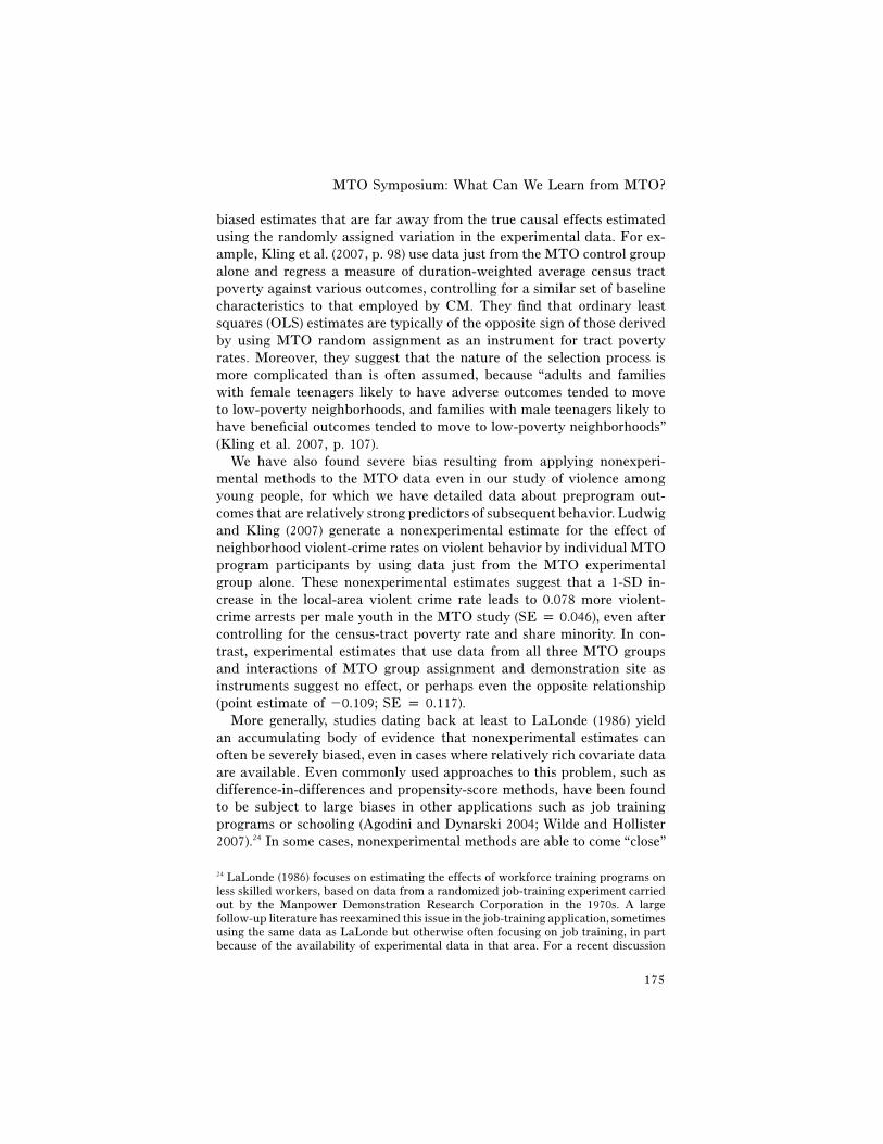
MTO Symposium: What Can We Learn from MTO?
175
biased estimates that are far away from the true causal effects estimatedusing the randomly assigned variation in the experimental data. For ex-ample, Kling et al. (2007, p. 98) use data just from the MTO control groupalone and regress a measure of duration-weighted average census tractpoverty against various outcomes, controlling for a similar set of baselinecharacteristics to that employed by CM. They find that ordinary leastsquares (OLS) estimates are typically of the opposite sign of those derivedby using MTO random assignment as an instrument for tract povertyrates. Moreover, they suggest that the nature of the selection process ismore complicated than is often assumed, because “adults and familieswith female teenagers likely to have adverse outcomes tended to moveto low-poverty neighborhoods, and families with male teenagers likely tohave beneficial outcomes tended to move to low-poverty neighborhoods”(Kling et al. 2007, p. 107).
We have also found severe bias resulting from applying nonexperi-mental methods to the MTO data even in our study of violence amongyoung people, for which we have detailed data about preprogram out-comes that are relatively strong predictors of subsequent behavior. Ludwigand Kling (2007) generate a nonexperimental estimate for the effect ofneighborhood violent-crime rates on violent behavior by individual MTOprogram participants by using data just from the MTO experimentalgroup alone. These nonexperimental estimates suggest that a 1-SD in-crease in the local-area violent crime rate leads to 0.078 more violent-crime arrests per male youth in the MTO study (SE p 0.046), even aftercontrolling for the census-tract poverty rate and share minority. In con-trast, experimental estimates that use data from all three MTO groupsand interactions of MTO group assignment and demonstration site asinstruments suggest no effect, or perhaps even the opposite relationship(point estimate of �0.109; SE p 0.117).
More generally, studies dating back at least to LaLonde (1986) yieldan accumulating body of evidence that nonexperimental estimates canoften be severely biased, even in cases where relatively rich covariate dataare available. Even commonly used approaches to this problem, such asdifference-in-differences and propensity-score methods, have been foundto be subject to large biases in other applications such as job trainingprograms or schooling (Agodini and Dynarski 2004; Wilde and Hollister2007).24 In some cases, nonexperimental methods are able to come “close”
24 LaLonde (1986) focuses on estimating the effects of workforce training programs onless skilled workers, based on data from a randomized job-training experiment carriedout by the Manpower Demonstration Research Corporation in the 1970s. A largefollow-up literature has reexamined this issue in the job-training application, sometimesusing the same data as LaLonde but otherwise often focusing on job training, in partbecause of the availability of experimental data in that area. For a recent discussion
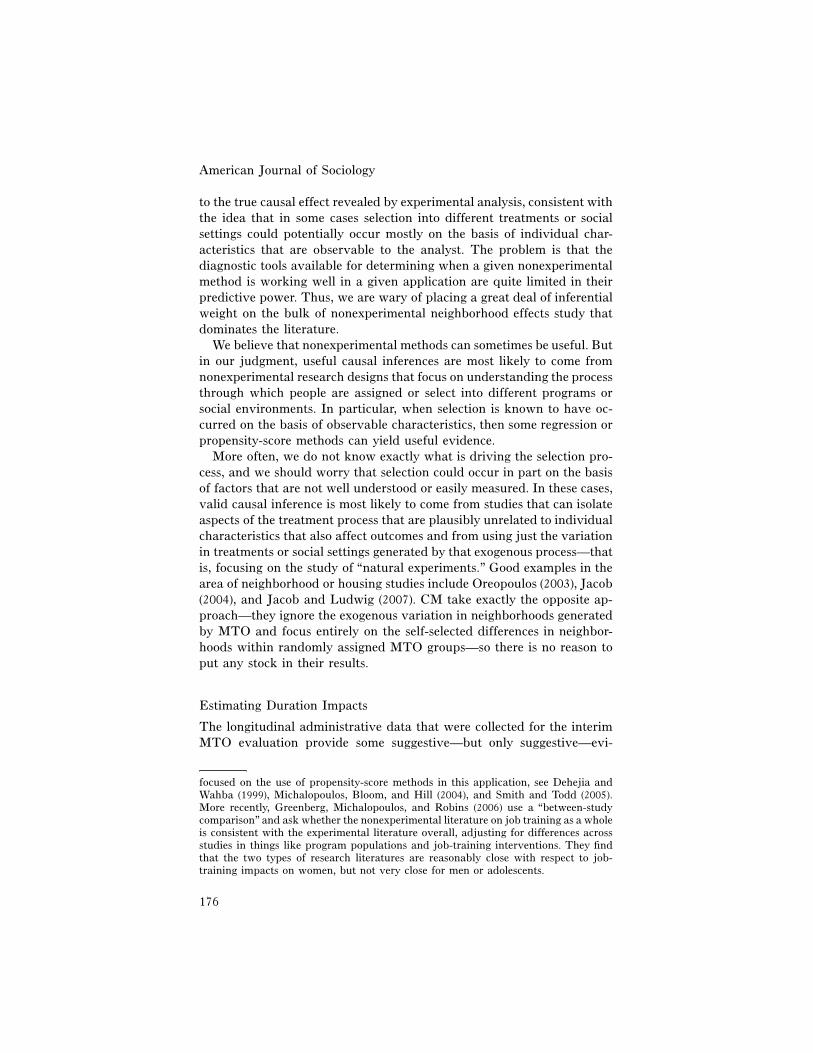
American Journal of Sociology
176
to the true causal effect revealed by experimental analysis, consistent withthe idea that in some cases selection into different treatments or socialsettings could potentially occur mostly on the basis of individual char-acteristics that are observable to the analyst. The problem is that thediagnostic tools available for determining when a given nonexperimentalmethod is working well in a given application are quite limited in theirpredictive power. Thus, we are wary of placing a great deal of inferentialweight on the bulk of nonexperimental neighborhood effects study thatdominates the literature.
We believe that nonexperimental methods can sometimes be useful. Butin our judgment, useful causal inferences are most likely to come fromnonexperimental research designs that focus on understanding the processthrough which people are assigned or select into different programs orsocial environments. In particular, when selection is known to have oc-curred on the basis of observable characteristics, then some regression orpropensity-score methods can yield useful evidence.
More often, we do not know exactly what is driving the selection pro-cess, and we should worry that selection could occur in part on the basisof factors that are not well understood or easily measured. In these cases,valid causal inference is most likely to come from studies that can isolateaspects of the treatment process that are plausibly unrelated to individualcharacteristics that also affect outcomes and from using just the variationin treatments or social settings generated by that exogenous process—thatis, focusing on the study of “natural experiments.” Good examples in thearea of neighborhood or housing studies include Oreopoulos (2003), Jacob(2004), and Jacob and Ludwig (2007). CM take exactly the opposite ap-proach—they ignore the exogenous variation in neighborhoods generatedby MTO and focus entirely on the self-selected differences in neighbor-hoods within randomly assigned MTO groups—so there is no reason toput any stock in their results.
Estimating Duration Impacts
The longitudinal administrative data that were collected for the interimMTO evaluation provide some suggestive—but only suggestive—evi-
focused on the use of propensity-score methods in this application, see Dehejia andWahba (1999), Michalopoulos, Bloom, and Hill (2004), and Smith and Todd (2005).More recently, Greenberg, Michalopoulos, and Robins (2006) use a “between-studycomparison” and ask whether the nonexperimental literature on job training as a wholeis consistent with the experimental literature overall, adjusting for differences acrossstudies in things like program populations and job-training interventions. They findthat the two types of research literatures are reasonably close with respect to job-training impacts on women, but not very close for men or adolescents.
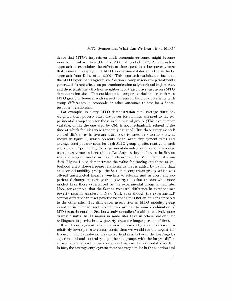
MTO Symposium: What Can We Learn from MTO?
177
dence that MTO’s impacts on adult economic outcomes might becomemore beneficial over time (Orr et al. 2003; Kling et al. 2007). An alternativeapproach to examining the effects of time spent in a low-poverty areathat is more in keeping with MTO’s experimental design is to use the IVapproach from Kling et al. (2007). This approach exploits the fact thatthe MTO experimental-group and Section 8 comparison-group treatmentsgenerate different effects on postrandomization neighborhood trajectories,and these treatment effects on neighborhood trajectories vary across MTOdemonstration sites. This enables us to compare variation across sites inMTO group differences with respect to neighborhood characteristics withgroup differences in economic or other outcomes to test for a “dose-response” relationship.
For example, in every MTO demonstration site, average duration-weighted tract poverty rates are lower for families assigned to the ex-perimental group than for those in the control group. (This explanatoryvariable, unlike the one used by CM, is not mechanically related to thetime at which families were randomly assigned). But these experimental/control differences in average tract poverty rates vary across sites, asshown in figure 1, which presents mean adult employment rates andaverage tract poverty rates for each MTO group by site, relative to eachsite’s mean. Specifically, the experimental/control difference in averagetract poverty rates is largest in the Los Angeles site, smallest in the Bostonsite, and roughly similar in magnitude in the other MTO demonstrationsites. Figure 1 also demonstrates the value for tracing out these neigh-borhood effect dose-response relationships that is added by having dataon a second mobility group—the Section 8 comparison group, which wasoffered unrestricted housing vouchers to relocate and in every site ex-perienced changes in average tract poverty rates that are somewhat moremodest than those experienced by the experimental group in that site.Note, for example, that the Section 8/control difference in average tractpoverty rates is smallest in New York even though the experimental/control difference in tract poverty for that site is not an outlier comparedto the other sites. The differences across sites in MTO mobility-groupvariation in average tract poverty rate are due to some combination ofMTO experimental or Section 8–only compliers’ making relatively moredramatic initial MTO moves in some sites than in others and/or theirwillingness to persist in low-poverty areas for longer periods of time.
If adult employment outcomes were improved by greater exposure torelatively lower-poverty census tracts, then we would see the largest dif-ference in adult employment rates (vertical axis) between the Los Angelesexperimental and control groups (the site-groups with the largest differ-ence in average tract poverty rate, as shown in the horizontal axis). Butin fact, the average employment rates are very similar in the experimental
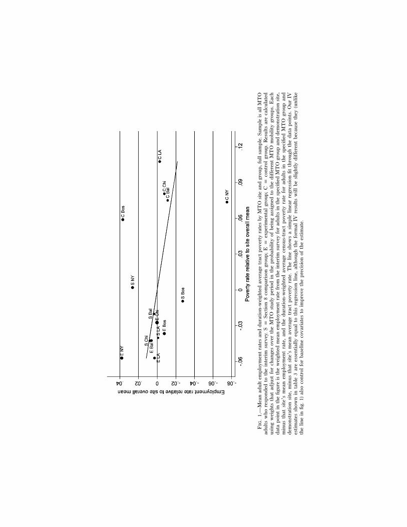
Fig
.1.
—M
ean
adu
ltem
plo
ymen
tra
tes
and
du
rati
on-w
eigh
ted
aver
age
trac
tp
over
tyra
tes
by
MT
Osi
tean
dgr
oup
,fu
llsa
mp
le.S
amp
leis
allM
TO
adu
lts
wh
ore
spon
ded
toth
ein
teri
msu
rvey
.S
pS
ecti
on8
com
par
ison
grou
p;
Ep
exp
erim
enta
lgr
oup
;C
pco
ntr
olgr
oup
.R
esu
lts
are
calc
ula
ted
usi
ng
wei
ghts
that
adju
stfo
rch
ange
sov
erth
eM
TO
stu
dy
per
iod
inth
ep
rob
abil
ity
ofb
ein
gas
sign
edto
the
dif
fere
nt
MT
Om
obil
ity
grou
ps.
Eac
hd
ata
poi
nt
inth
efi
gure
isth
ew
eigh
ted
mea
nem
plo
ymen
tra
tefr
omth
ein
teri
msu
rvey
for
adu
lts
inth
esp
ecifi
edM
TO
grou
pan
dd
emon
stra
tion
site
,m
inu
sth
atsi
te’s
mea
nem
plo
ymen
tra
te,
and
the
du
rati
on-w
eigh
ted
aver
age
cen
sus-
trac
tp
over
tyra
tefo
rad
ult
sin
the
spec
ified
MT
Ogr
oup
and
dem
onst
rati
onsi
te,
min
us
that
site
’sm
ean
aver
age
trac
tp
over
tyra
te.
Th
eli
ne
show
sa
sim
ple
lin
ear
regr
essi
onfi
tth
rou
ghth
ed
ata
poi
nts
.O
urIV
esti
mat
essh
own
inta
ble
3ar
ees
sen
tial
lyeq
ual
toth
isre
gres
sion
lin
e,al
thou
ghth
efo
rmal
IVre
sult
sw
ill
be
slig
htl
yd
iffe
ren
tb
ecau
seth
ey(u
nli
keth
eli
nein
fig.
1)al
soco
ntr
olfo
rb
asel
ine
cov
aria
tes
toim
pro
ve
the
pre
cisi
onof
the
esti
mat
e.

MTO Symposium: What Can We Learn from MTO?
179
and control groups in the Los Angeles site. The same dose-response logicsuggests that we should see a relatively small difference in employmentrates between the Section 8 and control groups in the New York site,since the group contrast in average tract poverty is smallest here comparedto all of the other treatment/control contrasts across the MTO sites. Butagain, that is not the case.
More generally, the regression line fit through the 15 site-group meansshown in figure 1 is downward-sloping but rather flat, suggesting thatthere is not much relationship between average tract poverty rates andemployment rates. This regression line through the site-group means isessentially what is estimated by a two-stage least squares procedure thatuses interactions between indicators for MTO demonstration sites andmobility group assignments as instrumental variables for average tractpoverty rate in a regression that has adult employment as the outcomeof interest.
With this approach, a neighborhood socioeconomic measure such asduration-weighted average tract poverty rates (POV) is viewed as a sum-mary index for a bundle of neighborhood characteristics that are changedas a result of MTO. Interactions between treatment-group assignments(e) and site indicators (S) are used as instrumental variables to isolate theexperimentally induced variation in POV across sites and groups, as inequation (1), where the main site effects are subsumed in X together withthe same standard set of baseline covariates controlled for by CM and inour own previous published work on MTO. Controlling for these baselinecovariates serves mainly to improve the precision of our estimates. Wealso use weights to adjust for changes over the course of the MTO ex-periment in the probability that subjects are randomly assigned to thethree MTO mobility groups (see Orr et al. 2003). The first-stage powerof our estimates is quite high: The F-test for the joint significance of theinstruments in first-stage equation (1), using the full sample, is equal to40.5 ( ). Table 4 shows the results for l2 from a separate estimationP ! .001of equations (1) and (2) for different outcomes and analytic samples, whereY in equation (2) is some behavioral outcome of interest.
POV p (e # S)m � Xb � � . (1)1 1 1
Y p POVl � Xb � � . (2)2 2 2
Table 4 shows the results of estimating this IV procedure for differentoutcome measures (rows) and analytic samples (columns), where each cellreports the coefficient from a different two-stage least squares regression.We do not see much support for the idea that more pronounced andsustained changes in tract poverty rates translate into improved adult

American Journal of Sociology
180
TABLE 4Instrumental Variable Estimates for Effects of Tract Poverty on
MTO Adult Economic Outcomes
Outcome MeasureFull
Sample
Random Cohort Assignment
Early Late
Psychological distress (K-6index) . . . . . . . . . . . . . . . . . . . . . .239* (.117) .112 (.174) .284* (.142)
Employed . . . . . . . . . . . . . . . . . . . �.159 (.161) �.253 (.234) �.016 (.202)Weekly earnings . . . . . . . . . . . . 29 (71) �59 (106) 164 (88)TANF receipt . . . . . . . . . . . . . . . .147 (.151) .411 (.216) �.150 (.195)Food stamps receipt . . . . . . . . .028 (.160) .290 (.238) �.244 (.200)N . . . . . . . . . . . . . . . . . . . . . . . . . . . . . 3,664 1,823 1,841
Notes.—The table presents point estimates and SEs (in parentheses) using interactions ofMTO treatment group and MTO demonstration site as instrumental variables for duration-weighted postrandomization average tract poverty rate. These estimates control for a set ofstandard baseline covariates related to the adult’s educational attainment, baseline employmentstatus, and social program participation and use weights to adjust for a change in the random-ization rates across MTO groups during the course of the program period (see Orr et al. [2003]for details).
* .P ! .05
economic outcomes. We see slightly larger point estimates for labor marketoutcomes for early cohorts relative to those derived using either the fullsample or just the late cohorts, but this may simply reflect the fact thatthe economic outcomes for earlier cohorts of program participants responddifferently than do those of later cohorts (as demonstrated in table 3). Incontrast, the estimate in the top row of table 4 for the full MTO sampleindicates a large and statistically significant improvement in adult mentalhealth (reductions in Ronald Kessler’s K-6 index) from more time spentin lower-poverty areas.
It is important to note that our IV estimates in table 4 cannot beinterpreted literally as the effects of changing neighborhood poverty rateson the economic outcomes of MTO adults. Our tract poverty measurecaptures the effects of the entire bundle of community attributes that arecorrelated with tract poverty and that influence economic outcomes. Withonly 10 instruments, our ability to isolate the distinct effects of separateneighborhood attributes on outcomes is necessarily limited (see Kling etal. [2007] for an extended discussion).25
25 Ludwig and Kling (2007) show that there is enough variation across MTO sites andgroups to distinguish the effects of tract SES composition from tract racial compositionon violent-crime arrests of MTO participants. When we try to instrument for bothtract SES and racial composition with adult economic outcomes as the dependentvariable of interest, the estimated effects of duration-weighted tract poverty changeonly slightly in comparison to the results in table 4, while the estimated effects fortract share minority are quite imprecise.
MTO Symposium: What Can We Learn from MTO?
181
CONCLUSIONS
Empirical evidence on the existence and nature of neighborhood effectsis important, given that fully 7.9 million people lived in high-povertycensus tracts in 2000 (Jargowsky 2003). Housing and other social policiesaffect the concentration of poor families in highly disadvantaged neigh-borhoods. There is great demand from policy makers across the countryto understand whether and how neighborhood environments affect thelife chances of low-income families, and, if so, what to do about it. TheMTO experiment provides the best opportunity to date for answeringsome of these questions.
Our disagreement with CM concerns the best way to analyze the MTOdata and what inferences can and cannot be supported from these anal-yses. CM end their article with an argument for how analysts should usethe MTO data in the future: “Measuring the effect of a voucher offer isvital to assessing the experimentally sound results of the policy demon-stration. However, if MTO data are used to measure neighborhood effects,different assumptions and techniques should be considered,” using non-experimental models that “sacrifice MTO’s experimental design” (p. 139).We believe that their assessment of the ability of experimental MTOanalysis to be informative about neighborhood effects is misguided andthat their specific prescriptions for future MTO analyses are likely togenerate erroneous conclusions.
Experimental estimates of the effects of MTO voucher offers and uti-lization are useful for understanding the scope of neighborhood effectson behavioral outcomes for low-income families, currently living in someof our nation’s most disadvantaged communities, who wish to relocate—a highly policy-relevant group. Random assignment of families to differentMTO mobility groups, some of which are offered housing vouchers, gen-erates large differences in average neighborhood trajectories across groupswith respect to such community attributes as socioeconomic composition,safety, disorder, informal social control, and the social ties of MTO familiesthemselves. Sociological and other theories predict that these neighbor-hood attributes influence behavior.
Large neighborhood differences across MTO groups persist despite thefact that only some families assigned to the experimental group movedthrough the program, MTO moves generated relatively little residentialintegration by race and ethnicity, and some families moving in conjunctionwith the program eventually moved on to worse neighborhoods. None ofthese facts bias our ITT or TOT estimates of the effects of the differingneighborhood bundles caused by random assignment to the MTO treat-ment. If neighborhood environments affect behavior four to seven yearsafter baseline among the sort of people who enroll in MTO, then these
American Journal of Sociology
182
neighborhood effects ought to be reflected in ITT and TOT impacts onbehavior.
Thus, MTO tells us something important about the effects of mobilityinterventions in the medium run for an important population of low-income families living in very distressed urban areas. It shows us thatmoving out of a disadvantaged, dangerous neighborhood into more af-fluent and safer areas does not have detectable impacts on economicoutcomes four to seven years out. However, such neighborhood movesdo have important effects on other self-reported measures of the well-being of program participants (which surely count for something), on adultmental health and some physical health outcomes, and on violent behavioramong young people.
Nonexperimental analyses of the type conducted by CM reintroduceall of the selection bias problems that MTO was designed to overcome.Moreover, their model confounds changes in neighborhood effects as fam-ilies stay in low-poverty areas longer with neighborhood effects that varyby random assignment cohort in MTO, as suggested by the fact thatcontrolling for random-assignment cohort greatly reduces the magnitudeof CM’s estimated effects of time spent in low-poverty areas. And theirresults provide no support for their arguments about the importance ofintegrating by both race and social class.
We should emphasize that the MTO estimates are informative onlyabout the effects of mobility programs like MTO on the types of low-income families who would choose to participate in such programs. MTOis silent on the effects of involuntary mobility programs, which is animportant point, given ongoing HOPE VI activities across the country todemolish some of our highest-poverty housing projects.
Readers are also cautioned against trying to draw inferences from MTOabout interventions designed to change disadvantaged neighborhoodsthemselves, rather than relocating residents to other areas. Compared withMTO, this type of intervention requires much greater knowledge on thepart of policy makers about what specific neighborhood attributes mattermost for improving outcomes. If policy makers focus on changing thewrong set of neighborhood attributes, the impacts of a place-based in-tervention could be less beneficial than what we see in MTO. The effectsof a place-based program might also differ from MTO because the formermight be less disruptive to the existing social networks of families.Whether that would lead to more- or less-beneficial impacts compared toMTO is not obvious as a conceptual matter; for some families, existingsocial ties may hinder rather than help their economic and other outcomes,and so the net effect of leaving these networks unchanged will dependin part on the distribution of positive and negative network connections.
We agree with CM that it is possible that MTO impacts on participating
MTO Symposium: What Can We Learn from MTO?
183
families might grow larger over time, if families become more sociallyintegrated into their new communities or are able to accumulate morehuman capital as a result of their improved mental health. The best wayto test this hypothesis is additional data collection—from administrativerecords on MTO families for a longer time period and a second wave ofdetailed survey reports from MTO participants. This possibility suggeststhe great importance of continuing to follow MTO families into the future,a point that CM are sure to join our team in endorsing.
APPENDIX
To help clarify the issues around selection bias, we review Heckman’s(1996) framework for thinking about how randomized experiments helpovercome selection. Let represent some economic, health, or other out-Y1i
come for a given low-income adult (i) if he uses a voucher to move intoa low-poverty area, and let represent the outcome this person wouldY0i
receive if he did not have a voucher and so remained in a high-povertyarea. Let di p 1 if the person uses a voucher; otherwise, di p 0. Theessential problem for social scientists is that a given individual either usesa voucher or does not; we cannot observe both and at the sameY Y1i 0i
point in time for the same person, and so we must rely on differentstatistical methods to estimate the missing data on counterfactualoutcomes.
Assume that the potential outcomes for people in both states (low pov-erty with voucher and high poverty) are functions of observable variables(Xi) as well as other variables that are usually not observed in the standarddata sets that are typically used to estimate neighborhood effects on labormarket or other outcomes (Ui):
Y p g (X ) � U , E(U ) p 0; (A1)1i 1 i 1i 1i
Y p g (X ) � U , E(U ) p 0. (A2)0i 0 i 0i 0i
The outcome we actually observe for a given person is Y p d Y �i i 1i
, and so by substituting this into equations (A1) and (A2) and(1 � d )Yi 0i
defining , we getD p (Y � Y )i 1i 0i
Y p g (X ) � d {[g (X ) � g (X )] � (U � U )} � Ui 0 i i 1 i 0 i 1i 0i 0i
p g (X ) � d D � U . (A3)0 i i i 0i
People might benefit from living in a lower-poverty neighborhood witha housing voucher because, for instance, labor market outcomes for highschool dropouts (an observable characteristic in Xi) are better in areas
American Journal of Sociology
184
that are closer to less-skilled job opportunities; this would be representedby the difference . Alternatively, they might have improvedg (X ) � g (X )1 i 0 i
labor market outcomes because living in a lower-poverty area reduces anunobserved variable that makes it difficult to work, such as stress; thiswould be reflected by the difference .U � U1i 0i
Equation (A3) is essentially a stylized version of the sort of nonexper-imental regression analysis that dominates the neighborhood effects lit-erature. Instead of a simple dichotomous indicator for living in a low-poverty or high-poverty area, most studies regress some outcome ofinterest against a series of neighborhood variables that tend to be thosethat are easily measured from the decennial census, such as census-tractpoverty rates or tract %minority. The key econometric issues are similarif d is a vector of continuous neighborhood measures rather than a binaryscalar. The set of control variables (X) generally includes standard de-mographic variables such as age, education, and race and may also includemore involved individual-level background variables, such as parents’education levels, family income, or even more detailed measures of familyfunctioning.
Selection bias occurs when di is not orthogonal to the unobserved factorsthat influence outcomes (U1i and U0i in the equations above), so that
. Selection bias is difficult to avoid with non-E[U � U Fd p 1, X ] ( 01i 0i i i
experimental analysis, because individual characteristics that affect theoutcome variable will inevitably be left out of the regression. Moreover,the direction of this bias is difficult to predict by theory alone.
Randomization solves the selection problem by causing the variationin neighborhood of residence to occur for reasons that are uncorrelatedwith individuals’ potential outcomes. Building on the notation introducedabove, let if a person (i) is randomly assigned to the MTO treatmente p 1i
group and so is eligible to receive a MTO voucher, while if thee p 0i
person is assigned to the MTO control group. The main experimentalresults come from comparing the outcomes of all of the families random-ized into the treatment group with those of all the families randomizedinto the control group, calculated mechanically by regressing Y against eand adjusting for baseline covariates X to improve precision. This ITTanalysis measures the effect of offering families a housing voucher andhousing mobility counseling.
To see why partial compliance does not introduce selection bias in theexperiment, use the potential outcomes framework from above and let
represent the probability that someone with observable char-P(d p 1FX )i i
acteristics Xi makes an MTO move in equation (A4). If MTO treatment-group assignment has no effect on those who do not move through theprogram (represented as ), thenE[YFd p 0, e p 1] p E[YFd p 0, e p 0]i i i i i i
the change in outcomes (Y) induced by assignment to the experimental

MTO Symposium: What Can We Learn from MTO?
185
rather than the control group is equal to the mean effect of MTO moveson those who move (represented as , and known moreE(D Fd p 1, X )i i i
generally as the TOT effect), multiplied by the share of people who willmake MTO moves if given the chance, .P(d p 1FX )i i
Y p g (X ) � [E(D Fd p 1, X )]P(d p 1FX )ei 0 i i i i i i i
� (U � U )P(d p 1FX )e � U . (A4)1i 0i i i i 0i
The key virtue of random assignment is that the indicator for assign-ment to the treatment group, e, will be independent of the backgroundcharacteristics of MTO sample respondents, X, the potential outcomespeople would experience with and without a voucher, Y0 and Y1, and theprobability of leasing up if offered a voucher, . The fact thatP(d p 1FX)only some MTO families assigned to the experimental group comply withtheir treatment assignment and relocate through the program does notintroduce any bias to our estimates, because this propensity to movethrough MTO is balanced across families assigned to both the experi-mental and control groups. Similarly, random assignment balances thepropensity to stay in a low-poverty area rather than move back to aslightly higher-poverty area, and so subsequent mobility after familiesmake their initial MTO moves also does not introduce any bias to theITT estimate.
A more subtle point is that there is some “selection bias” in equation(A4), in the sense that the baseline covariates, X, are not independent ofthe unobserved determinants of potential outcomes U1 and U0 (Heckman1996). In our previous published estimates for MTO impacts on outcomes(e.g., Kling et al. 2005; Kling et al. 2007), we controlled for baseline char-acteristics to improve the precision of our ITT and TOT estimates, butthe fact that these baseline measures may be correlated with unobservabledeterminants of postrandomization outcomes means that we cannot in-terpret the coefficients on the baseline covariates as causal effects. But,as Heckman (1996) notes, this type of “selection bias” (correlation of back-ground controls with the error term) is balanced across randomly assignedgroups, and so it will not affect our ability to generate an unbiased ITTestimate. The ITT estimate compares all members of the treatment groupto all members of the control group, and so by construction does not sufferfrom selection bias itself.
REFERENCES
Aber, J. Lawrence, Jeanne Brooks-Gunn, and Greg J. Duncan, eds. 1997. NeighborhoodPoverty: Context and Consequences for Children, vols. 1 and 2. New York: RussellSage Foundation.
Agodini, Roberto, and Mark Dynarski. 2004. “Are Experiments the Only Option? A
American Journal of Sociology
186
Look at Dropout Prevention Programs.” Review of Economics and Statistics 86 (1):180–94.
Bartus, Tamas. 2005. “Estimation of Marginal Effects using margeff.” Manuscript. http://www.bke.hu/bartus/pdf/bartus_2005_sj.pdf
Bloom, Howard S. 1984. “Accounting for No-Shows in Experimental EvaluationDesigns.” Evaluation Review 8 (April): 225–46.
Bloom, Howard S., et al. 1996. “The Benefits and Costs of JTPA Title II-A Programs.”Journal of Human Resources 12 (3): 549–76.
Chamberlain, Gary. 1984. “Panel Data.” Pp. 1247–1320 in Handbook of Econometrics,vol. 2. Edited by Zvi Griliches and Michael D. Intriligator. Amsterdam: North-Holland.
Clampet-Lundquist, Susan, and Douglas S. Massey. 2008. “Neighborhood Effects onEconomic Self-Sufficiency: A Reconsideration of the Moving to OpportunityExperiment.” American Journal of Sociology 114 (1): 107–43.
Dehejia, Rajeev, and Sadek Wahba. 1999. “Causal Effects in Non-experimental Studies:Re-evaluating the Evaluation of Training Programs.” Journal of the AmericanStatistical Association 94 (448): 1053–62.
Ellen, Ingrid Gould, and Margery Austin Turner. 2003. “Do Neighborhoods Matterand Why?” Pp. 313–38 in Choosing a Better Life? Evaluating the Moving toOpportunity Social Experiment, edited by John Goering and Judith D. Feins.Washington, D.C.: Urban Institute Press.
Glaeser, Edward L., Bruce Sacerdote, and Jose A. Scheinkman. 1996. “Crime andSocial Interactions.” Quarterly Journal of Economics 111 (2): 507–48.
———. 2003. “The Social Multiplier.” Journal of the European Economic Association1 (2–3): 345–53.
Goering, John, Judith D. Feins, and Todd M. Richardson. 2003. “What Have WeLearned about Housing Policy and Poverty Deconcentration?” Pp. 3–36 in Choosinga Better Life: Evaluating the Moving to Opportunity Social Experiment, edited byJohn Goering and Judith D. Feins. Washington, D.C.: Urban Institute Press.
Greenberg, David H., Charles Michalopoulos, and Philip K. Robins. 2006. “DoExperimental and Nonexperimental Evaluations Give Different Answers about theEffectiveness of Government-Funded Training Programs?” Journal of PolicyAnalysis and Management 25 (3): 523–52.
Heckman, James J. 1996. “Randomization as an Instrumental Variable.” Review ofEconomics and Statistics 78 (2): 336–41.
Jacob, Brian A. 2004. “Public Housing, Housing Vouchers and Student Achievement:Evidence from Public Housing Demolitions in Chicago.” American EconomicReview 94 (1): 233–58.
Jacob, Brian A., and Jens Ludwig. 2007. “The Effects of Housing Vouchers onChildren’s Outcomes.” Working paper. University of Michigan, Ford School ofPublic Policy.
Jargowsky, Paul A. 2003. “Stunning Progress, Hidden Problems: The Dramatic Declineof Concentrated Poverty in the 1990s.” Policy brief. Brookings Institution,Washington, D.C.
Jencks, Christopher, and Susan E. Mayer. 1990. “The Social Consequences of GrowingUp in a Poor Neighborhood.” Pp. 111–86 in Inner-City Poverty in the United States,edited by L. E. Lynn, Jr. and M. G. H. McGeary. Washington, D.C.: NationalAcademies Press.
Kain, John F. 1968. “Housing Segregation, Negro Employment and MetropolitanDecentralization.” Quarterly Journal of Economics 82 (2): 175–97.
Katz, Lawrence F., Jeffrey R. Kling, and Jeffrey B. Liebman. 2001. “Moving toOpportunity in Boston: Early Results of a Randomized Mobility Experiment.”Quarterly Journal of Economics 116:607–54.
Keels, Micere, Stefanie DeLuca, Greg J. Duncan, Ruby Mendenhall, and James
MTO Symposium: What Can We Learn from MTO?
187
Rosenbaum. 2005. “Fifteen Years Later: Can Residential Mobility Programs Providea Long-Term Escape from Neighborhood Segregation, Crime, and Poverty?”Demography 42 (1): 51–73.
Kling, Jeffrey R., Jeffrey B. Liebman, and Lawrence F. Katz. 2007. “ExperimentalAnalysis of Neighborhood Effects.” Econometrica 75 (1): 83–119.
Kling, Jeffrey R., Jens Ludwig, and Lawrence F. Katz. 2005. “Neighborhood Effectson Crime for Female and Male Youth: Evidence from a Randomized HousingVoucher Experiment.” Quarterly Journal of Economics 120 (1): 87–130.
LaLonde, Robert J. 1986. “Evaluating the Econometric Evaluations of TrainingPrograms with Experimental Data.” American Economic Review 76:604–20.
Leventhal, Tama, and Jeanne Brooks-Gunn. 2000. “The Neighborhoods They Live In:The Effects of Neighborhood Residence on Child and Adolescent Outcomes.”Psychological Bulletin 126 (2): 309–37.
Ludwig, Jens, Greg J. Duncan, and Paul Hirschfield. 2001. “Urban Poverty andJuvenile Crime: Evidence from a Randomized Housing-Mobility Experiment.”Quarterly Journal of Economics 116 (2): 655–80.
Ludwig, Jens, Greg J. Duncan, and Joshua C. Pinkston. 2005. “Housing MobilityPrograms and Economic Self-Sufficiency: Evidence from a RandomizedExperiment.” Journal of Public Economics 89 (1): 131–56.
Ludwig, Jens, and Jeffrey R. Kling. 2007. “Is Crime Contagious?” Journal of Law andEconomics 50 (3): 491–518.
Ludwig, Jens, Helen Ladd, and Greg J. Duncan. 2001. “The Effects of Urban Povertyon Educational Outcomes: Evidence from a Randomized Experiment.” Pp. 147–201in Urban Poverty and Educational Outcomes, edited by William Gale and JanetRothenberg Pack. Brookings-Wharton Papers on Urban Affairs. Washington, D.C.:Brookings Institution Press.
Luttmer, Erzo F. P. 2005. “Neighbors as Negatives: Relative Earnings and Well-Being.”Quarterly Journal of Economics 120 (3): 963–1002.
Matthews, Jay. 2007. “Neighborhoods’ Effect on Grades Challenged: Moving StudentsOut of Poor Inner Cities Yields Little, Studies of HUD Vouchers Say.” WashingtonPost, August 14. Page A2.
Mendenhall, Ruby, Stefanie DeLuca, and Greg Duncan. 2006. “NeighborhoodResources, Racial Segregation and Economic Mobility: Results from the GautreauxProgram.” Social Science Research 35 (4): 892–923.
Michalopoulos, Charles, Howard S. Bloom, and Carolyn J. Hill. 2004. “Can PropensityScore Methods Match the Findings from a Random Assignment Evaluation ofMandatory Welfare-to-Work Programs?” Review of Economics and Statistics 86:156–79.
Moffitt, Robert A., ed. 2003. Means-Tested Transfer Programs in the United States.Chicago: University of Chicago Press.
Newhouse, Joseph P., and IEG (the Insurance Experiment Group). 1993. Free for All?Lessons from the RAND Health Experiment. Cambridge, Mass.: Harvard UniversityPress.
Oreopoulos, Philip. 2003. “The Long-Run Consequences of Growing Up in a PoorNeighborhood.” Quarterly Journal of Economics 118 (4): 1533–75.
Orr, Larry L., Howard S. Bloom, Stephen H. Bell, Fred Doolittle, Winston Lin, andGeorge Cave. 1996. Does Training for the Disadvantaged Work? Evidence from theNational JTPA Study. Washington, D.C.: Urban Institute Press.
Orr, Larry L., Judith D. Feins, Robin Jacob, Erik Beecroft, Lisa Sanbonmatsu,Lawrence F. Katz, Jeffrey B. Liebman, and Jeffrey R. Kling. 2003. Moving toOpportunity Interim Impacts Evaluation. Washington, D.C.: U.S. Department ofHousing and Urban Development, Office of Policy Development and Research.
Rosenbaum, James E. 1995. “Changing the Geography of Opportunity by Expanding
American Journal of Sociology
188
Residential Choice: Lessons from the Gautreaux Program.” Housing Policy Debate6 (1): 231–69.
Rubin, Donald B. 1980. “Comment on ‘Randomization Analysis of Experimental Data:The Fisher Randomization Test,’ by D. Basu.” Journal of the American StatisticalAssociation 75:591–93.
Rubinowitz, Leonard S., and James E. Rosenbaum. 2000. Crossing the Class and ColorLines: From Public Housing to White Suburbia. Chicago: University of ChicagoPress.
Sampson, Robert J., Jeffrey D. Morenoff, and Thomas Gannon-Rowley. 2002.“Assessing ‘Neighborhood Effects’: Social Processes and New Directions inResearch.” Annual Review of Sociology 28:443–78.
Sampson, Robert J., Stephen W. Raudenbush, and Felton Earls. 1997. “Neighborhoodsand Violent Crime: A Multilevel Study of Collective Efficacy.” Science 277 (5328):918–24.
Sanbonmatsu, Lisa, Jeffrey R. Kling, Greg J. Duncan, and Jeanne Brooks-Gunn. 2006.“Neighborhoods and Academic Achievement: Results from the Moving toOpportunity Experiment.” Journal of Human Resources 41 (4): 649–691.
Shadish, W. R. 2000. “The Empirical Program of Quasi-experimentation.” Pp. 13–36in Research Design: Donald Campbell’s Legacy, edited by L. Bickman. ThousandOaks, Calif.: Sage.
Shroder, M. 2002. “Locational Constraint, Housing Counseling, and Successful Lease-Up in a Randomized Housing Voucher Experiment.” Journal of Urban Economics51:315–38.
Smith, Jeffrey, and Petra Todd. 2005. “Does Matching Overcome LaLonde’s Critiqueof Non-experimental Estimators?” Journal of Econometrics 125:305–53.
Sobel, Michael E. 2006. “What Do Randomized Studies of Housing MobilityDemonstrate? Causal Inference in the Face of Interference.” Journal of the AmericanStatistical Association 101 (476): 1398–1407.
Solon, Gary, Marianne E. Page, and Greg J. Duncan. 2000. “Correlations betweenNeighboring Children in their Subsequent Educational Attainment.” Review ofEconomics and Statistics 82 (3): 383–92.
Turney, Kristin, Susan Clampet-Lundquist, Kathryn Edin, Jeffrey R. Kling, and GregJ. Duncan. 2006. “Neighborhood Effects on Barriers to Employment: Results froma Randomized Housing Mobility Experiment in Baltimore.” Pp. 137–87 inBrookings-Wharton Papers on Urban Affairs, edited by Gary Burtless and Janet R.Pack. Washington, D.C.: Brookings Institution Press.
Votruba, Mark E., and Jeffrey R. Kling. 2004. “Effects of Neighborhood Characteristicson the Mortality of Black Male Youth: Evidence from Gautreaux.” Working paperno. 491. Princeton University, Industrial Relations Section.
Wilde, Elizabeth Ty, and Robinson Hollister. 2007. “How Close is Close Enough?Evaluating Propensity Score Matching Using Data from a Class Size ReductionExperiment.” Journal of Policy Analysis and Management 26 (3): 455–78.
Wilson, William Julius. 1987. The Truly Disadvantaged: The Inner City, the Underclass,and Public Policy. Chicago: University of Chicago Press.