Policy Research

Infrastructure and Urban Development Department

The World Bank October 1992

WPS 998

What Determines Demand for Freight Transport?

Esra Bennathan Julie Fraser

and Louis S. Thompson

Long-run demand for freight transport is determined in closely similar ways in developed and developing market economies. Not, however, in the transitional socialist countries, where structural change is likely to bring far greater changes in rail freight activity than in road transport.

Policy Research Wo&ing Papers dissemmste the fmdings of work in pmgrea and mmumgethe exchange of ideas among Bank staff and all othexs intarsted in developent issues. These papers carry the names of the authors, reflect only their views, and should be used and cited accordingly The fmdings, interpretations. and conclusions are the authors’ own. They should not be attributed to the World Bank, its Board of Directors, its management. or any of its member countries.

policy Research

Transport

WPS 998

This paper - a product of the Transport Division, Infrastructure and Urban Development Department - is part of a larger effort in the department to develop quantitative aids for the evaluation of performance of infrastructure-related services, the design of policy, and the establishment of priorities. Copies of the paper are available free from the World Bank, 1818 H Street NW, Washington, DC 20433. Please contact Barbara Gregory, room SlO-049, extension 33744 (October 1992.29 pages).

Decisions about investments in the long-lived assets of transport infrastructure require some assumptions about prospective long-term demand from services using that infrastructure. To improve the basis for such predictions, Bennathan, Fraser, and Thompson estimated the long-run determinants of domestic freight transport, using single-equation regressions on a cross-section of data from “developed” (high- income), “developing” (low-income), and former socialist economies.

They also sought answets to two related questions. First, since statistics on national ton- kilometers of freight transport are much scarcer for developing than for developed countries, what is the scope for generalizing from data on high-income countries? Second, within what limits may one apply results obtained from data on market economies to the prospective evolu- tion of freight transport demand in the socialist transitional economies?

They report the following findings, subject to caveats related to the simple methodology used:

. For the sample of developed countries, and the merged samples of developed plus develop- ing countries, total ton-kilometers of freight transport (excluding transit) are adequately explained by two variables: a country’s area and total GDP. Ton-kilometers by road are chiefly explained by GDP; ton-kilometers by rail am explained by country area.

0 Road freight in developed and developing market economies shows very similar response

(in additional ton-kilometers) to variations in GDP. But the elasticity of demand for road ton- kilometers with regard to GDP should be about or above 1.25 for developing countries, com- pared with close to unity for the high-income countries.

l Demand for rail freight transport appears to be determined in closely similar ways in both groups of countries. Elasticity with GDP appears to be close to unity.

0 Judging from the narrow basis of evidence on socialist economies (China and the former USSR were excluded for technical reasons), transport demand was determined very differ- ently in their systems than in the market econo- mies. The contrasts are almost entirely ex- plained by the differences in the role of, and demand for, rail transport in the different eco- nomic systems.

The road sector of freight transport, on the other hand, conforms closely to norms in the market economies; the marginal response (additional ton-kilometer for additional GDP) and elasticity with respect to GDP, appear - on the available evidence -to be close to what is found for developed market economies.

* Jn short, structural change in the socialist economies is likely to bring about far greater changes in rail freight activity than in road transport.

The Policy Research Working Paper Series disseminates the findings of work under way in the Bank. An objective of the series is to get these findings out quickly, even if presentations are less than fully polished. The findings, interpretations, and conclusions in these papers do not necessarily represent official Bank policy.

Produced by the Policy Research Dissemination Center

Infrastwture and Urban Development Depaltment

The World Bank

FREIGHT TRANSPORT DEMAND: DETERMINANTS AND INTENSITY

Esra Bennathan Julie Fraser

Louis S. Thompson

CQNTENTS

Introduction and Summary . . . . . . . e . . . . . . . . . . . . . . . . . . . . . . D . . . . . . . i

1 -Qbject,MeaningoftheResultsandtheData ...................... 1 Specification ....................................... 1

Cross-section Coefficients: Meaning ........................ 1 TheData ......................................... . An Adjustment to Country Area .......................... .2

The Sample and Sample Selection .......................... 3 Collinearity.. ...................................... .

2 Results.. .......................................... ...6 The Regressions, and Order of Discussion ..................... 6 “Developed” and “Developing” Countries ..................... 6 “Developed” and “Socialist” Countries ...................... 10

A GDP in Dollars: Which Dollars? ............................. 17 B SampleData ......................................... .21 C Regression: F’ullReport ................................... 22 D Test for the Equality of Coefficients ........................... 29

TABLES In Text

Table 1: Regression Results - Total Tkm ............................ 7 Table 2: Regression Results - Road Tlcm ............................ 8

Table 3: Regression Results - Rail Tkm ............................ 9

In Annexes

Table A. la: Results of Regressing Ton-Kilometers on dollar GDP (converted first at MXR and then by PPP) . . . . . . . . . . . . . . . . . . . . 19

Table A. lb: Results of Regressing Ton-Kilometers on dollar GDP (after logarithmic transformation of the variables) . . . . . . . . , . . . . s . . 20

Paee 2 of 2 CONTENTS

In Text

Figure 1: Transport Ton-Km per $ of GDP (Road, Rail & Water) . . . . . . . . . . . . 11 Figure 2: RailShareofTruck + RailTraffic . . . . . . . . . . . . . . . . . . . . . . . . 13 Figure 3: Variation of Observed over Predicted Total Ton-Km (1) . . . . . . . . . . . . 14 Figure 4: Variation of Observed over Predicted Road Ton-Km (1) . . . . . . . . . . . . 15

In Annexes

Figure A. 1: ICP GDP vs. GDP Converted at Market Rates (dollars per capita) . . . . . 18

ACKNOWLEDGEMENTS

The cdmments and suggestions of Ms. Frida Johansen, Mr. Philip Blackshaw, Mr. Gregory Ingram, and Mr. Jan de Weille are gratefully acknowledged.

INTRODUCTI~NAND S-Y

THE QUESTIONS

. In this note we attempt to estimate the determinants of the domestic freight transport of countries from cross-section data. Our investigation is guided by an interest in three questions:

e Can the evolution of domestic demand for freight transport be predicted to a reasonably high level of explanation with a few readily available variables? For practical purposes, in decisions on sectoral investment allocations or as background parameters in decisions on individual investments or service projects, that would be a desirable outcome. Moreover, the small number of usable observations available for our study dictated strict economy in the number of explanatory variables.

0 Does the explanation differ in a significant way between high-income (“developed”) and lower-income (“developing “) countries? One would expect such differences if the structure of national production (e.g., industry vs agriculture) had an important effect on the demand for freight transport, independent of the effect of measured GDP.

l And does the explanation differ significantly according to economic system: between market economies and others? The formally centrally planned economies of Europe are known to be highly transport intensive. In designing schemes for the transformation and privatization of transport enterprises it is important to know whether such high (average) intensity expresses itself also at the margin, and equally for the different major modes?

Our results go some way towards answering these questions.

M~WHOD, DATA, AND LIMITATIONS

We investigated the domestic (non-transit) demand for freight transport with a single equation, regressing ton-kilometers on total GDP and country area, on the data of 33 countries.

Since the results are obtained from a cross-section study, they describe long-run behavior or demand for freight transport: the elasticities we obtain are long-run elasticities.

GDP was measured in international dollars as estimated by the International Comparison Project (i.e., converted at purchasing power parities). The chief effect of substituting GDP data converted to US dollars with market exchange rates is to lower significantly the elasticity of ton-

ii Introduction and Summary

kilometers with respect to GDP. The areas of Australia and Canada, both in our sample, were scaled down to allow for the vast tracts of empty land in each of their territories.

Our sample includes three mutually exclusive groups of countries: ‘developed’ and ‘developing’, categorized by GDP per capita, and socialist economies. The number of observations available for analysis is small because estimates of ton-kilometers are a relatively scarce statistic. China, the United States and the USSR (for which data are available) had to be omitted from the sample. Being very large in both territorial extent and populations, their presence in the samples raised the correlation between our two explanatory variables -- GDP and area --to unsafe levels. Retaining them in the samples would have biased the coefficient estimates: the separate effects of GDP and area could not have been reliably estimated. Faced with the small number of observations for the groups of ‘developing’ and ‘socialist’ countries, we carried out the regressions on three sub-samples: developed countries, developed + developing countries, and developed + socialist countries.

The significance of differences in coefficients between the sub-samples was investigated by testing for the equality of coefficients in the underlying samples (‘developed’, ‘developing’ and ‘socialist’).

The major caveat attaching to our results arises from the two-way relation between ton- kilometers of transport and GDP which is ignored in our single-equation model. Our results may therefore be affected by a simultaneity bias. They can only be taken for what they purport to represent on the assumption that GDP in the countries was not constrained by shortage of freight transport.

RESULTS

Performance of the Model

The explanatory power of the model, measured by the R2s, was generally high when all variables were entered in their natural values, and somewhat lower in the logarithmic version. The explanatory power was least when the “socialist” countries were included in the samples. In the regressions on the samples of “developed” and “developing” countries the R2s were .85 or higher and thus satisfactory by usual standards.

Dominant Variables

Separating by mode of transport, the explanation of t-kms by road is dominated by the In the determination of rail transport, it is country m (or variations in area) GDP variable.

that dominates.

Introduction and Summary . . . 1l.l

‘6Developed9p and 6‘Developingpp Market Econo~es

Demand for ton-kilometers by the three surface modes (road, rail and water) appears to have a higher (positive) elasticity with respect to GDP in the poorer countries, but the difference is not strictly significant. Sharper results are obtained from an analysis by mode.

For road freight, the elasticity of demand with respect to GDP, given country area, rises markedly when the developing countries are added to the sample of developed countries. The difference is significant and we infer a substantially higher elasticity for the developing countries: very likely with a lower bound of 1.25. At the margin, however, another Dollar of GDP generates almost the same number of ton-kilometers of freight in either group of countries, and therefore irrespective of GDP per capita,

In the explanation of ton-kilometers of rail transport, on the other hand, none of the differences that appear between ‘developed’ and ‘developed plus developing’ country samples turn out significant: demand is determined by a similar process irrespective of differences in GDP, and country area dominates the explanation. Allowing for area, the elasticity of ton- kilometers with respect to country GDP may be taken as unity.

‘6Developedpp + ‘6SociaM9y Countries Sample

The addition of only five “socialist” to 17 “developed market” countries may not permit the idiosyncracies of freight transport demand under socialist organization of the economies to show through adequately in our regressions. But there are nevertheless strong hints of the type and direction of the divergences. Pirst, the elasticity of t-kms with respect to GDP drops markedly when the five socialist economies are added to the developed market economies: apparently, transport demand is governed by different laws in the different systems. Second, a clear contrast is evident between the behavior of freight transport by road and by rail. When applied to road transport, the explanatory power of the model is hardly affected by the addition of socialist countries to the sample, and the estimated (simple) coefficients on the independent variables are only slightly changed. Not so in the case of rail: the model loses explanatory power9 and the size of the estimated coefficients on the explanatory variables are about halved when the socialist economies are admitted into the sample. By this evidence, the road sector of freight transport, but not the rail sector, conforms rather closely to the norms of the market economies. The conclusion is fully consistent with the known share of rail in socialist freight transport which exceeds the corresponding share in market economies by a large factor.

I OBJECT,MEANINGOFTHERESULTS, ANDTHEDATA

1. In this paper we seek to explain total ton-kilometers of freight in a cross-section of countries, in terms of two intuitively appropriate variables: a country’s total GDP, and its area. In this selection of explanatory variables we have been deliberately austere or simplistic. The object was to discover, if possible, relationships between variables that are readily ascertained, in a form that is readily understood.

2. Before presenting the results an explanation is in order of what meaning we can attach to them, as well as a description of the data and of data-related problems.

Specification

3. We have estimated the determinants of ton-kilometerst’ of freight by Ordinary Least Squares regression with a single equation. Notionally, this is a demand equation: demand for ton-kilometers (the dependent. variable) is determined by GDP and area (the independent variables). GDP, however, is not exogenous with respect to freight transport. It is itself produced by transport. To account for this input characteristic of freight transport would require the formulation of a simultaneous equations model, and a solution of the reduced form (explaining ton-kilometers in terms of, say, area and the national stocks of labor and capital).2’ The results would not be easy to interpret, nor is it easy to obtain values for the appropriate exogenous variables for many countries. We therefore stayed with the single equation model, thus accepting the risk of simultaneity bias in the estimated coefficients. Concretely, the results represent what they claim to represent on the assumption that transport capacity (infrastructure and services) forms no constraint on GDP.

Cross-section Coefficients: Meaning

4. Abstracting from a potential simultaneity bias, the results need to be understood with due regard to the meaning of the cross-section approach. Cross-section analysis is intended to reveal equilibrium relations. The coefficient on GDP purports then to show the increase in ton- kilometers (millions) for another (million) dollars of GDP, given the country’s area, and after full adjustment of the country’s economy, factor use and location of production and consumption to that addition to GDP. The coefficient does not tell us about the reaction of ton-kilometers to cyclical variation in GDP: for that we would need to study time series. Similarly, the elasticities that we obtain have to be seen as long-run elasticities.

II A ton-kilometer or tlcm represents one metric ton moved one kilometer.

21 An alternative method for dealing with the problem would be the use of instrumentable variables.

2 Chapter 1

The Data

5. Information on country area (in km2) is readily obtained and presumably quite accurate. The area variable nevertheless presents us with a special problem, to be discussed in the section immediately following.

6. GDP data are adjusted for purchasing power and expressed in international dollars, as provided by the International Comparison Project.3’ The exceptions are Bulgaria, Czechoslovakia, and the USSR for which there are no corresponding ICP GDP figures. As a best estimate, for Bulgaria and Czechoslovakia we have used data provided by L.W. International Financial Research, Inc. From PlanEcon (as quoted in The Economist) we took the figure for the USSR though the country was omitted from the regression analysis for reasons to be given later.

7. Measuring GDP in a common currency according to the ICP methodology rather than by methods that involve market exchange rates obviously affects the regression results. In Annex A we discuss the effect of this approach.

8. Dollar GDP numbers were taken for the year 1989. Where ton-kilometers data were only available for another (earlier) year, an adjustment was made (via GDP in national currency and the general GDP deflator) so as to represent GDP for that earlier year at 1989 prices.

9. Our ton-kilometers refer to domestic (i.e. non-transit) transport performed by modes other than air and pipeline. As a statistic, this is unlikely to be better than GDP estimates, and probably rather more problematic. Rail transport data are presumably relatively accurate. The difficulty of estimation affects road and water transport for which sources and method differ between countries. The definitions and reporting of Yransit” also vary among countries.

10. Transit traffic is neither a function of the transit country’s GDP, nor of its area. We have therefore sought to exclude the transit component from the total ton-kilometers of countries with a substantial amount of transit traffic. The available data allowed all or part of transit traffic to be removed from the data for Austria, Belgium, Finland, Hungary, Netherlands, Norway, and Yugoslavia.

An Adjustment to Country Area

11. GDP and Area are obviously not the only explanations that one thinks of for the volume of a country’s freight transport. They may be so for some countries, but not for all. More comprehensive formulations might yield better (or more widely based and applicable) regression

31 For the latest set of these estimate-s, see Summers, R. and Alan He&on, “The Penu World Table (Mark 5): An expanded set of international comparisons, 1950-1988,” Ouarterlv Journal of Economics, Vol. C!VI, No. 2, May 1991.

Chapter 1 3

results, if the attending statistical risks can be avoided. Bringing in further variables would, however, conflict with our pragmatic rule of simplicity. But in considering the Area variable we could not altogether avoid compromising the rule, by allowing some role to another variable, that of density of settlement.

12. . Several countries in our sample cover large areas but have very low average density. This is the case of Canada, Australia, Finland, Norway and Sweden, the first two being at the lower extreme. The developed parts of Canada cover not more than one-third of its area, and in the interior parts of Australia -- about 85 percent of its total area -- density is 0.5 persons per square km. In these two cases we reduced total country area to reflect the existence of large expanses substantially void of activity that could give rise to freight transport. Canada’s area was reduced by 75 percent and Australia’s, by 80 percent. Both are countries with high incomes per head but populations that are small relative to their large areas. The effect of thus scaling down their areas has been to raise the regression coefficient of Area and to sharpen the distinction between Area and GDP as determinants of total ton-kms of freight. Adjustments to other country area figures were not done since the effects on our results would be minor.

The Sample and Sample Selection

13. An immediate consequence of the difficulty of estimating ton-kilometers for a country’s total freight transport is the relative scarcity of such data. Developed countries tend to provide the information, but it is available for only some developing countries. Therefore, in composing and dividing the sample for purposes of comparison between different classes of countries, we were necessarily constrained by the supply of data.

14. Our total sample consisted of the 36 countries listed in Annex B. For reasons to be given later, we removed 3 countries from the regression set, leaving 33. We categorized the remaining countries broadly according to GDP per capita and economic system, as follows:

(a)

(b)

(c)

17 high and upper-middle income economies (“Developed, market”)

11 lower-middle and low income market economies (“Developing, market”)

5 transitional socialist economies of Europe (“Socialist”)

15. Samples (b) and (c) are rather small. For purposes of comparison we therefore limited our regression analysis to sample (a) on its own, (a) +@) merged, and (a) -t(c) merged. It follows that any differences between the determinants of ton-kilometers in “developed” and “developing” or “socialist” economies have to be inferred from variations in the enlarged samples relative to the basic developed market sample.

4 Chapter 1

16. When differences appear between the coefficients estimated on sample (a) and the amalgamated samples (a + b) or (a + c) we have to establish that the difference is significant (i.e., unlikely to be due to chance). We do this by testing for the equality of coefficients (the Chow test) at the .05 level of significance. Annex D presents the steps in the test.

Collinearity

17. Since we are seeking to explain ton-kilometers of freight in a cross-section of countries by two variables, area and GDP, it is necessary to ask whether the two exogenous variables are related: could either stand in for the other? In that case the regression results would be biased. One should expect to find multicollinearity if it were the case that (a) country area is correlated across the sample with country population, and (b) the variation in area across the sample is greater than the variation in GDP per capita.

18. We started investigating the question by looking at the largest countries (in terms of unadjusted area) within our data set: USSR, China, USA, Canada, Australia and India. The smallest of those, India, is not quite 4 times as large in area as the next biggest, Pakistan. India has a very large population but a very low income per head. Canada and Australia, while high- income countries, have relatively small populations and hence relatively small GDP (Canada’s is about 70 percent of India’s). That leaves the USA with large area, large population and high income per head; and the (former) USSR with the largest area, a population larger than that of the USA and with an income per head that may be a small fraction of USA incomes but a large multiple of India’s, and China, with an area somewhat greater than the USA. The latest ICP estimate of China’s GDP per capita (1988) seems unduly high at $2,472. But even after scaling this down by 30 percent, China’s total GDP would amount to $1.9 trillion, second only to that of the USA.

19. We investigated the correlation between area and GDP in our various samples:

(a) In our sample of 18 developed countries, the correlation coefficient (r) between area and GDP dropped precipitously when the USA was removed from the sample: from .94 to .22.

We then formed a sample of developed and socialist countries. With both the USA and the USSR in the sample, the simple correlation coefficient between area and GDP was .52. Removing only the USA, it rose to .63; removing only the USSR, it went up to .95. The two therefore operate as counterweights: the area of the USSR is 2.4 times that of the USA, but the USA (according to our numbers) has 3.8 times the GDP. While a correlation coefficient of .52 does not contain a major threat of bias in the estimated coefficients, we wanted to stay on the side of caution, and therefore removed both countries from the sample. The effect was to lower r to .27, an innocuous level.

Chapter 1 5

(c) Similarly, in the sample of “developed + developing” countries, the presence of China (assigned to this group because of systemic differences with other centrally planned economies) raised the coefficient of correlation between GDP and Area from .40 to .82.

20. . Our conclusion is that the safest regression results would be obtained from samples that excluded the USA, the USSR and China. Our discussion of results will therefore be based on those reduced samples but the coefficients from estimation on unreduced samples are shown in Annex C.

6

2 RESULTS

THE REGRESSIONS, AND ORDER OF DIEUSSION

21. We performed our regressions separately for:

l ton-kilometers by rail, road and water (Table l), l ton-kilometers by road (Table 2), 0 ton-kilometers by rail (Table 3).

22. Each regression was performed twice over. In the first version, the variables are measured in the normal form. In the second, we enter the (natural) logarithms of the values. For ease of discussion, we refer to the coefficients resulting from the first model as simple coefficients, and to those from the logarithmic transformation, as elasticties.

23. In discussion, we concentrate first on results for “developed” and “developed + developing n countries. After that, we turn to the sample of “developed + socialist” countries.

Ton-kilometers by Three Modes

24. The estimates of the simple coefficients in Table 1, panels B and C, are all highly significant by the test of the t-ratio. Next, the explanatory power of the model, in terms of the adjusted R2 statistic, rises markedly when ton-kilometers are regressed on area and GDP rather than separately on each of the two regressors. That, we will argue, results from lumping together freight transport by road and by rail.

25. The most interesting information that one hopes to obtain from the regression of ton-kms by all (three) modes concerns the elasticity of demand with respect to GDP. Here, unfortunately, the results are ambiguous. On the other hand, proceeding from the sample of developed countries, we find the elasticity rising from 1.06 to 1.24. This suggests that the elasticity rises systematically, as GDP declines in the cross section. But the difference of the coefficient in the two underlying samples (developed and developing countries) turns out to be just below the critical point for significance (Annex D). That would imply that the same process generates demand for freight transport in the two groups of countries, differences in coefficients being probably due to chance. But as we move on to analyzing the determinants of demand by mode of transport, a clearer picture emerges.

Chapter 2

II Table 1: Regression Results - Total Tkm

t V&able = LN(lKhfY

Road Freight

26. Of the two independent variables, it is GDP that determines variations in ton-kilometers of road transport (Table 2). While the simple coefficient on area has the right sign, it is generally not significant and only serves to improve the explanation of ton-kilometers marginally, if at all. The coefficient on GDP, however, is highly significant and accordingly displays useful characteristics. First, it is virtually the same whether area is included in the regression or not: it gives a high level of explanation when used on its own. Second, it has very similar values in the smaller (“developed” countries) and the larger (“developed + developing” countries) samples. For either group of countries it would be legitimate to say that another million (international) Dollars added to GDP adds another 170,000 ton-kilometers to road freight transport, irrespective of the country’s income per capita, and practically irrespective of its area.

27. These identical (or almost identical) absolute additions to road freight service are, however, associated with different long-run elasticities. The difference is significant. Poorer countries have fewer road ton-kilometers per dollar of GDP than the richer ones. For the sample of 17 “developed” countries, the partial elasticity of ton-kilometers by road with respect to GDP is about unity (1.02). For the larger sample, including the poorer countries, it is well

Chapter 2

above unity (1.28). The contrast suggests (though our observations are too few to demonstrate) that the long-run elasticity is substantially higher in the group of developing countries than in the high-and-middle-income group. We hazard the proposition that the value of the elasticity in developing countries has, say, 1.25 as its lower limit.

Table 2: Regression Results - Road Tkm

Rail Freight

28. Demand for rail ton-kms (Table 3) is governed by essentially similar determinants in our samples of developed and developing countries. Of the two independent variables, it is clearly country area that provides the dominant explanation of inter-country variation. The explanatory power of GDP when taken on its own is very low and the estimate of the simple coefficient on GDP is normally not significantly different from zero. Adding GDP to Area in the regressions does practically nothing for the model’s power of explanation (the R2s).

29. By the test of R2 and t-ratio, our model seems no less adequate as an explanation of inter- country variations of rail freight than of road freight. But the almost total failure of GDP to enter into the explanation so far is nevertheless surprising and somewhat disappointing: there appears to be no growth effect in the use of railways. One naturally thinks of other factors that

Chapter 2 9

are likely to enter into the explanation of the inter-country differences in rail freight and are not caught in our model.

30. Railways are normally the chosen mode for the long-haul transport of basic bulk commodities. But adding national output of coal, lignite and iron ore to our independent variables yields insignificant results. Again, there is the historical factor: railways developed long before trucking, and hence before the networks of main roads, reached their present extent. We therefore entered the ratio of paved road length to country area as another explanatory variable. The sign on the coefficient of this ratio was negative, as expected. The coefficient estimate itself, however, was not significant.

31. Some indication of the effect of GDP on rail freight is, however, provided by the estimated elasticities. Logarithmic formulation lowers the explanatory power of our model (the R2) but the estimated coefficients on both area and GDP are significant, and of a size that agrees with intuition. The elasticity of rail ton-lcms with respect to area is somewhat lowered when the poorer countries are added to the set of “developed” countries. The GDP elasticity, however,

10 Chapter 2

rises markedly and is of the size that one expects: well below unity in the sample of middle- and-high income countries, and only little above unity for the enlarged set that includes the low- income countries. For developing countries, failing drastic changes in transport policy, one may expect rail freight to rise not much faster than GDP.

Transport Intensity

32. The socialist economies of Europe have long been known for their high transport intensity. Recent analysis, motivated by the search for methods of reforming the economies after their turn from socialist organization, has revealed the full extent of their transport intensity.4’ No unique explanation can be advanced for what is apparently the joint result of high industrial concentration, large activity in investment and construction, an absence of market relations and of market-based decisions on location, output and investment. The average transport intensity in the countries is declining, but remains high by the standards of Europe’s market economies (Figure 1). This high avenge intensity (a high ratio of ton-kilometers to GDP) is the background to the marginal relations shown by regression analysis.

Elasticities

33. The eccentrically large volume of ton-kilometers of freight in the socialist economies shows through in the elasticity estimates. From each of the three modes (all modes, road, rail), we obtain elasticities of ton-kilometers with respect to GDP which move in opposite directions when we merge the sample of “developed” countries, first with “developing” countries and then, with “socialist” countries. In the first case, the elasticity rises, in the second case it falls. To illustrate, we excerpt from Table 1 the elasticities for ton-kilometers by all three modes:

Elasticity w.r.t.

Developed countries

Developing Socialist + countries or + countries

Area .22 .19 .23

GDP 1.06 1.24 .94

41 Em Bennathan, Jeffrey Gutman and Louis Thompson, “Reforming and Privatizing Poland’s Road Freight Industry,” The World Bank, WPS 750, August 1991; Em Bennathan, Jeffrey Gutman and Louis Thompson, “Reforming and Privatizing Hungary’s Road Haulage,” The World Bank, WPS 790, October 1991.

Chapter 2 11

Figure 1 Transport Ton-Km per $ of GDP

(Road, Rail & Water)

( ) Area, 000 Km2

USSR (22,272)

Poland (305)

CSFR (125)

China (9,597)

Canada (2,305)

Bulgaria (Ill)

USA (9,167)

Hungary (92)

India (2,973)

Yugoslavia (255)

Spain (499)

Holland (34)

Sweden (412)

Belgium (30)

W. Germany (244)

U.K. (242)

Italy (294)

France (546)

Austria (63)

32

‘8

4

2

L

0 1 2 3 4 5

Tonne-Km per $ of GDP GDP is Purchasing Power Adjusted

12 Chapter 2

While the difference between the elasticities for the two underlying samples of developed and developing countries just misses the conventional 5 percent level of significance, the contrast in the deviations nevertheless agrees with intuition. It is simply the other side of the coin of high transport intensity in the (former) socialist economies. The “developing” countries are poorer than the “developed” countries, and have fewer ton-kilometers per Dollar of their GDP. As between the two groups, transport intensity rises with GDP. The “socialist” countries, on the other hand, are poorer than the “developed” countries but have a higher average transport intensity. In comparing ‘socialist’ and ‘developed’ countries, therefore, transport intensity does not rise with GDP.” The cross-section elasticity (with respect to GDP) accordingly rises as we add “developing” to “developed” countries, but declines as we add the “socialist” countries. To obtain a truer relationship between ton-kilometers and GDP across the latter sample, one would have to introduce a “socialist factor” as a separate independent variable in the regression.

Road and Rail

34. The simple coefficients on what we showed to be the dominant explanations of ton- kilometers by the two different modes - GDP for road and Area for rail - are closely similar across our three country samples. At the margin, therefore, freight carriage responds in a similar way to the identified determinants (or sources of demand), in the different groupings. But if the explanatory power of our model is measured in terms of the coefficient of determination (the adjusted R2) a strong contrast appears between “socialist” ton-kilometers by road and by rail. For the road mode, the R2 obtained from the different samples are practically of the same size. For the rail mode, however, the R2 drops precipitously as we move from the first two country samples to the one that includes the socialist economies: from .85 for sample B to .66 in sample D. In the case of roads, our model then explains as much of the variance of ton-kilometers in the “developed + socialist” sample as in the samples of “developed + developing” countries. But that is patently not true of ton-kilometers by rail. The comparatively low R2, and the comparatively large constants in the rail equations when the socialist countries are inserted in the sample is evidence of a strong “socialist factor” in the demand for rail haulage, not caught in the model as we formulate it.

35. This result is consistent with the share of rail in the combined ton-kilometers of road and rail in the former socialist economies. By the standards of Europe’s market economies, the share of rail is abnormally high (Figure 2). The main features of socialist freight transport that appear from a comparison with Europe’s market economies are shown in Figures 3 and 4. We first attempt to predict the total freight transport demand of socialist and developing countries by applying the coefficients estimated on our sample of developed countries. The result, in Figure 3, is consistent underprediction of demand in the socialist countries. Performing the same prediction, but only for road freight demand, we find no characteristic differences between developed, socialist and developing countries (Figure 4).

51 This argument is intuitive. To make it rigorous we should need to demonstrate that “developing” or “socialist” countries are on average poorer than “developed” countries in terms of dollar per ktli2.

Chapter 2 13

Figure 2 Rail Share of Truck + Rail Traffic

1 ) Area, 000 Km2

USSR (22,272)

CSFR (125)

Poland (305)

China (9,597)

Canada (2,305)

lndia (2,973)

USA (9,167)

Hungary (92)

Bulgaria (111)

Sweden (412)

Austria (83)

Yugoslavia (255)

France (546)

Belgium (30)

W. Germany (244)

Holland (34)

U.K. (242)

Italy (294)

Spain (499) i- , i-

20 40 60 80 100

Percent

66

60

59

!!!!!!I 69

(Transit traffic not included.)

14 Chapter 2

Figure 3 Variation of Observed over Predicted Total Ton-Km (1)

Philippines

Pakistan

Thailand -

Turkey -

Sweden -

Sri Lanka -

France -

Greece -

Tunisia -

India -

Australia -

Italy -

Finland -

Great Britain -

Canada -

Austria -

Spain -

China -

W. Germany -

Portugal -

Korea -

Denmark -

Yugoslavia -

USA -

Ireland -

Netherlands -

USSR -

Belgium -

Poland -

Hungary -

CSFR -

Bulgaria -

I i

(200) (50)

Percent

Developing

(1) lOO*(Actual-Predicted)/Actual Based on sample of developed countries.

Chapter 2 15

I

Figure 4 Variation of Observed over Predicted Road Ton-Km (1)

Norway - Korea -

Ireland - Austria -

Denmark - Tunisia -

China - Thailand - Pakistan -

India - Sweden - Greece - France -

Canada - Portugal -

USSR - CSFR -

Netherlands - Great Britain -

W. Germany - Hungary -

Turkey - Poland -

USA - Yugoslavia -

Finland - Italy -

Belgium - Australia - Bulgaria -

Spain - ._L

(200) (50) Percent

Developing Socialist

(1) 1 OO*(Actual-Predicted)/Actual Based on sample of developed countries.

16 Chapter 2

36. Our conclusion is that the road freight sector of the former socialist countries, in terms of its volume of output and the determinants of its output, conforms reasonably closely to the norms of Europe’s market economies. The appropriate statistical test confirms that ton-kms of road freight are determined in a similar way in developed, developing and socialist economies. Abnormally high transport intensity in the former socialist countries has its main cause in an abnormally large demand for rail freight. In the longer run, with the transformation of the economies, one expects transport intensity to decline. Technology, pricing and general transport policy will determine the pace of decline and the way in which it will be shared by road and rail. But it seems unavoidable that rail, and with it the railway establishment, will face the larger share of change.

17

ANNEXA GDPm DOLLARS: ~~%IICHDOLLARS?

Purchasing Power Parity vs. Market Exchange Rate

(0 Most of the GDP data that entered our regressions in this paper were expressed in International Dollars, estimated by the International Comparison Project (ICP) on the basis of purchasing power parities (PPP). That was done for all 28 “developed” and “developing” countries in our sample, and for 3 of the 5 “socialist” countries. But many multi-country, cross- section studies still employ national income or GDP figures converted into US Dollars at prevailing market exchange rates (MXR) or some simple transformation (e.g., n-year averages) of market rates6’

(ii) The chief difference between the results of the two methods of conversion -- between PPP and MXR conversion -- is in the relative levels of countries’ GDP rather than in growth rates. PPP conversion tends to raise the incomes of poorer countries relative to those with higher incomes. This effect appears clearly in our sample of 28 “developed” and “developing” countries (Figure A. 1).

(iii) Conversion of GDP by purchasing power parity takes account of relative prices, and of relative quantities of products and activities in a way that market exchange rates cannot reflect. That is the economic case for preferring ICP estimates of GDP. But practitioners still tend to use, and think in terms of, GDP data converted by MXR into US Dollars. We therefore repeat some of our regressions, substituting GDP in US Dollars at MXR, and comparing the results obtained with alternative GDP estimates.

“Developed + Developing” Countries

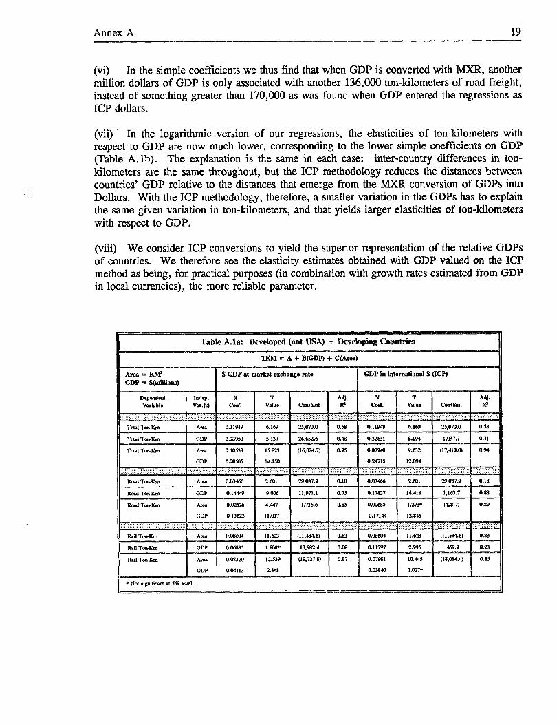
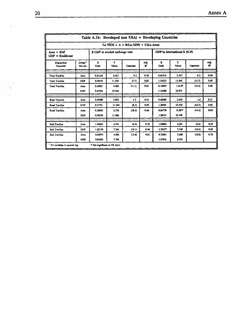
(iv) In Table A.la we present side by side the results of regressing ton-kilometers (total, road, and rail) on Dollar GDP, converted first at MXR and then by PPP. In Table A. lb, we compare the results of regressions after logarithmic transformation of the variables.

w The explanatory power of the model (the R’s) is hardly affected by switching from one specification of GDP to the other. The result of converting GDP at MXR is primarily to lower the effect of GDP on ton-kilometers of freight, and, secondarily, to raise somewhat the size of the Area effect. As a consequence, the differential dominance of GDP and Area in the explanation of ton-kms is much less visible when GDP is converted at MXR.

61 World Bank & GNP estimates allow for relative changes in the price levels of each country and the US but convert also with an (averaged) market exchange rate for the US Dollar.

18 Annex A

Figure A. 1 ICP GDP vs. GDP Converted at Market Rates

(Dollars per capita)

ICP GDP p.c.

25,000

20,000

15,000

10,000

5,000

0 0 5,000 10,000 15,000 20,000 25,000

GDP p.c. Converted at Market

Exchange Rates

Annex A 19

(vi) In the simple coefficients we thus find that when GDP is converted with MXR, another million dollars of GDP is only associated with another 136,000 ton-kilometers of road freight, instead of something greater than 170,000 as was found when GDP entered the regressions as ICP dollars.

(vii) . In the logarithmic version of our regressions, the elasticities of ton-kilometers with respect to GDP are now much lower, corresponding to the lower simple coefficients on GDP (Table A. lb). The explanation is the same in each case: inter-country differences in ton- kilometers are the same throughout, but the ICP methodology reduces the distances between countries’ GDP relative to the distances that emerge from the MXR conversion of GDPs into Dollars. With the ICP methodology, therefore, a smaller variation in the GDPs has to explain the same given variation in ton-kilometers, and that yields larger elasticities of ton-kilometers with respect to GDP.

(viii) We consider ICP conversions to yield the superior representation of the relative GDPs of countries. We therefore see the elasticity estimates obtained with GDP valued on the ICP method as being, for practical purposes (in combination with growth rates estimated from GDP in local currencies), the more reliable parameter.

Table A.Ba: Developed (not WA) + Developing Comtries

TKM = A + B(GDFj + C(Area)

20 Annex A

II Table A.lb: Developed (not USA) + Developing Countries 1

LnTKM=A+B&nGDP)fC(LnAra)

$ GDP at market exchange rate GDP in hMmationd $ (ICP)

Annex B 21

(ooo,ow toMt&Lll) Wlww &a (ooo) Tkd GDP/ country Road Water Rail Total Frt ICP GDP AREA Popul. SGDP Capita SOWX

1 1988 Australia 85000.0 0.0 81,000.0 166,OCO.O 228,455,976 1,523,586 16,765 0.73 13,627.O 1 1988 Austria 3 1985 Bangladesh 1 1988 Belgium 2 1988 Bulgaria 1 1988 Canada 3 1988 China 2 1988 Czechoslovakia 1 1985 Denmark 1 1985 Finland 1 1988 France 1 1988 Great Britain 1 1985 Greece 2 1988 Hungary 3 1987 India 1 1985 Ireland 1 1988 Italy 3 1981 Korea 3 1985 Malawi 3 1980 Morocco 1 1988 Netherlands 1 1985 Norway 3 1988 Pakistan 3 1980 Philippines 2 1988 Poland 1 1985 Portugal 1 1988 Spain 3 1987 SriLanka 1 1988 Sweden 3 1978 Thailand 3 1985 Tunisia 3 1988 Turkey 1 1988 USA 2 1988 USSR 1 1988 W. Germany 2 1988 Yugoslavia

Country Codes:

9,500.o 98.0 2,478.1 1,376.7

28,807.O 5,005.o 17,442.5 2,162.O 99,471.0

322,000.0 310,400.O 23,767.5 5,248.0

8,300.O 0.0 20,092.8 1,7@4.3

111,800.5 6644.0 129800.0 59300.0

12.096.0 0.0 14,640.o 2,046.O

120,780.5 10,980.O 4,498.2 0.0

157.600.0 194.5 11,400.o 9,400.o

166.8 9.2 LO80.9 3,779.o

33,069.O 29345.0 6,599.2 0.0

31,724.O 0.00 7,170.o 8,740.O

39,240.o 1,394.o 12,698.0 0.0

133,000.5 1,105.o 0.0

22,611.O 19,500.o 3,060.O 5,668.7 0.0

55,233.4 9,717.0 1,027,828.0 635.209.0

507,994.S 251,181.5 149,232.o 44,710.o 29,650.5 4,456.0

11,213.O 734.2

7,694.0 17,585.5

263,689.0 987,800.O

75,294.5 1,700.o 8,102.g

53,767.5 18,OOO.O

704.0 21,732.O

234,241.O 601.8

19,663.O 13,900.o

102.0 3,787.6 3,200.5 2.905.4 7,828.0

360.0 122,204.o

1,302.O 11,716.O

195.0 18,687.O 2,650.O 1,693.3 8,036.6

1,513,377.0 3,924,800.5

61,180.O 26,067.O

20.811.0 100,360.989 82,730 7,598 0.21 13,208.g 4,589 0 94,816,244 133,910 112,000 0.05 846.6

41,506.O 129,833,753 30,230 9,886 0.32 13,133.l 37,190.o 52,013,OOO 110,550 9,001 0.72 5,778.6

363,160.O 491641,079 2,305,244 26,302 0.74 18‘692.2 1,620,200.0 2,088,191,306 9,596,960 1,083,887 0.78 1.926.6

104,310.o l2&9gu.000 125,460 15,641 0.82 8,118.g 10,000.0 70,762,018 42,370 5,132 0.14 13,788.4 29,900.o 64,569,159 305,470 4,974 0.46 12,981.3

172,212.O 783,405,079 545,630 56,119 0.22 13,959.7 207,lOO.O 787,637,771 241,590 57,270 0.26 13,753.l

12,800.O 66,510,917 130,800 10,039 0.19 6,625.3 38,418.O 65,776,lOO 92,340 10,587 0.58 6.212.9

366,001.6 712,323,901 2,973,190 833,000 0.51 855.1 5,lOO.O 38,144,620 68,890 3,537 0.13 10.784.5

177,457.5 776,168,OOO 294,020 57,537 0.23 13,489.g 34,700.o 136,558,545 98,190 42,380 0.25 3,222.2

277.9 4,952,524 94,080 8,230 0.06 601.8 8,647.5 46,113,257 446,300 24,567 0.19 1,877.O

65,614.5 193,858,248 33,940 14,828 0.34 13,073 8 9.504.6 64,337,322 307,860 4,215 0.15 15,263.g

39,552.0 178,102,396 778,720 109,950 0.22 1,619.S 16,270.O 120,877,752 298,170 61,224 0.13 1,974.4

162,838.0 188,627,693 304,510 38,061 0.86 4,955.g 14,000.0 66,690,306 91,640 10,333 0.21 6,454.l

144716.5 395,752,565 499,400 39,161 0.37 10.105.8 1,300.o 34549,370 64,740 16,779 0.04 2.059.1

41,298.O 130,265,237 411,620 8,485 0.32 15,352.4 25,210.O 109,174,608 511,770 55,200 0.23 1,977.8

7,362.0 27,201,780 155,360 7,988 0.27 3,405.3 72,986.g 250,000,654 770,760 54,899 0.29 4,553.8

3,176,414.0 4,991,909,799 9,166,600 248,000 0.64 20,128.7 4,683,976.5 1,304,700,000 22,272,OOO 287,664 3.59 4,535.5

255,122.O 896,957,492 244,280 61,337 0.28 14.623.4 60,173.5 125,184,663 255,400 23,707 0.48 5,280.5

1. Developed Countries 2. Socialist Countries 3. Developing Countries

Sources of GDP data: 1. World Bank, World Development Report 1991, Table 30, pg 262-263, and The World Bank, World Tables 1991. 2. L.W. International Financial Research, Inc., “Occasional Papers Nos. 115-119 of the Research Project on National Income ln East Central

Europe, Table 15, pg 28., New York, NY 1991 3. The Economist, January 12, 1991, page 65 (quoting PlanEcon). 4. Central Bank of Ireland Annual Report, OECD Economic Outlook and World Bank, World Development Report 1991, Table 30, p. 263. 5. Summers, R. and Alan Heston, “The Penn World Table (Mark 5): An Expanded Set of International Comparisons, 1950-1988. Quarterly

Journal of Economics, Vol. CVI, No. 2, May 1991. Note:

GDP figures are based on 1989 ICP GDP per capita figures provided in World Development Report 1991, Table 30. This number is adjusted to the data year by applying a GDP deflator algorithm. ICP (International Comparison Program) estimates are expressed in “international dollars” which are obtained by special conversion factors designed to equalize purchasing powers of currencies in the respective countries. This note excludes Bulgaria, Czechoslovakia, and the USSR which were supplied in sources 2 and 3 above.

22 Annex C

Dependent Variable = Total Tkm (in millions) (Total Road, Rail, Water Tonne-Km)

Regression Analysis #I Area = KM2

GDP = PCP Intern’1 $ (mil)

GDP 0.21835 1 0.02732 ) 7.993 1 0.0000 1 I I

Annex C 23

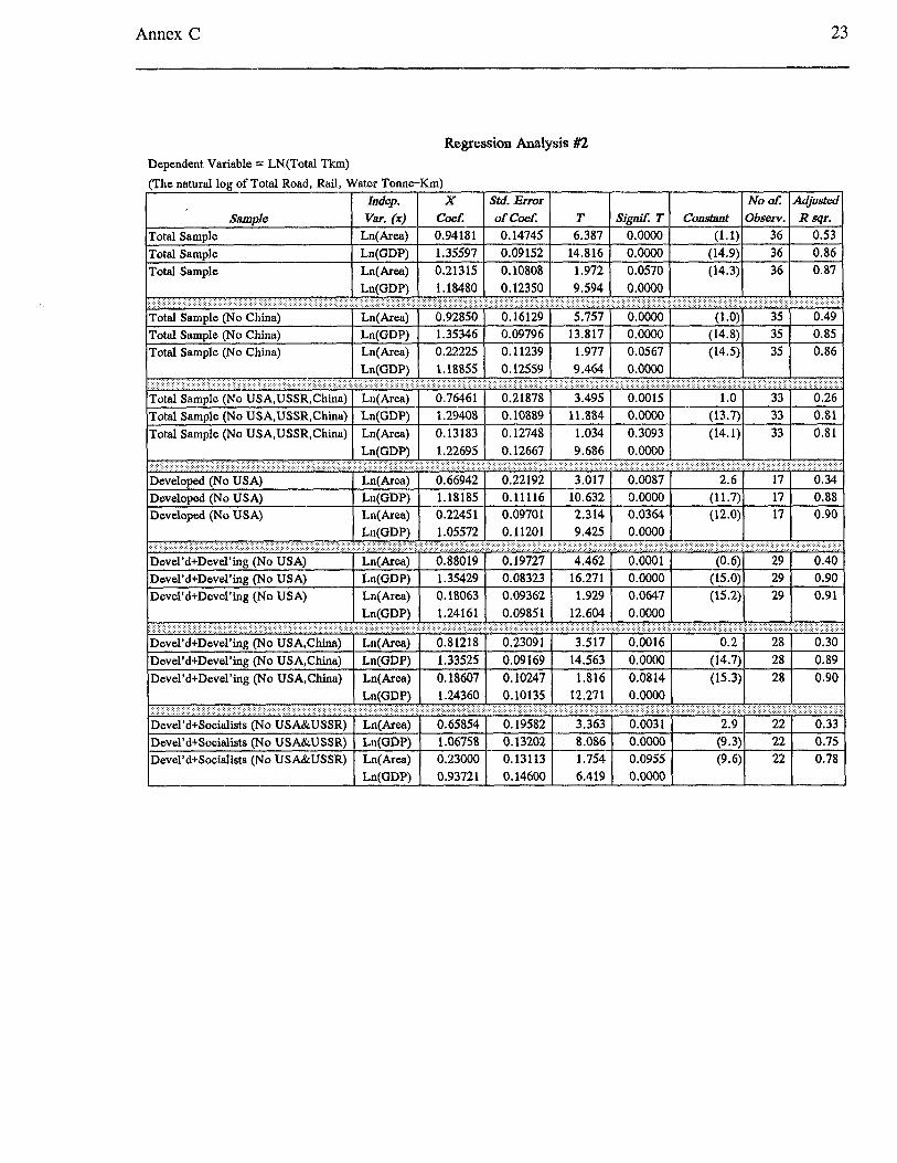
Regression Analysis #2 Dependent Variable = LN(Total Tkm)

(The natural log of Total Road, Rail, Water Tonne-Km)

Indep. x Std. Error No of. Adjusted Samule of CoeL T Sienif. T Constant Observ. Rsar.

1 Develooed INo USA> 1.18185 1 0.11116 1 10.632 1 O.OOOQ 1 111.7‘)) 17 I 0.88 I [i5kveiiped (No USA) ( Ln(Area) 1 0.22451 1 0.09701 1 2.314 1 0.0364 l l7 I 0.90 I

1 Ln(GDP) ( 1.05572 ... ,.I .,., ., .\. . . ;...,. :: .,., ..> . . . . . . ‘. . . . .:: :.:,:, _:“. ;.?,:::;$<: :: .....i....‘_._~ _“A,,,. :., .::::::, ,, _.‘. :: :‘::. .‘.‘. .’ . . . . 2. .,.... .‘.‘, ,,,., .: . . . . . . ‘.I? ,,,, .:‘/::~ ..y..:. j:::::: ., ., ; .,.,. . . Devel’d+Devel’ing (No USA) 1 Ln(Area) 1’ 0.88019 Devel’d+Devel’ing (No USA) 1 Ln(GDP) 1 1.35429

, . ,, Devel’d+Socialists (No USA&USSR) Ln(Area) 0.23000 0.13113 1.754 0.0955 ;9.6; 22 0.78

Ln(GDP) 0.93721 0.14600 6.419 0.0000

24 Annex C

Dependent Variable = Road Tkm Regression Analysis iK3

Area = KM2

Annex C 25

Dependent Variable = Ln (Road Tkm)

Regression Analysis #4

hdep. X std. Error NOOK Adjusted Sample var. (x) cod of cod T Signif T Constaot Observ. Raqr.

Total Sample Ln(Area) 0.75611 0.14781 5.115 0.0000 0.5 36 0.42 Total Sample Ln(GDP) 1.22350 0.08033 15.231 0.0000 (13.0) 36 0.87

1 Total Sample 1 Ln(Are.a) 1 0.00721 1 0.10029 1 0.072 1 0.9431 1 (13.O)l 36 I 0.86 I

/Total Sample (No

1 Ln(GDP) ,., .:.,.:...: . . . . .: . . . . . . . :... .,..: . . . . . . . . . . ,.:. :.:.:.::.:.:.:.:., ,.::;I):: .:. ,/ .:,:,:: :,:. ::, .:., ./:.:. .:..., ..,.. ..,. ,... . . . . . . .,.,...,.,.... :.:.:.:.:..:.:. China) Ln(Area) China) Ln(GDP) China) Ln(Area)

0.08504 1 0.10324 1

10.625 1 0.0000 ..:: :,:.: :::)::,.:?,’ . . . . . . . . . . . .,., ‘.:,:::::~,.:.::,:::.::::::::,j ,.,. .,...,.:. . . . . . . . .: . . . . . . . . ,,:. y::::

4.675 0.0000 14.660 0.0000 0.269 0.7900

1 Ln(GDP) 1 1.22618 1 0.11537 1 10.628 I 0.0000 I ..I. ........,, .,..,... :.,.> ,.... ~~.,.,.... ..,.,,.,..... .,.,., :.: ::.,:,,.:.::,.: ,,.. .I... . . . .:.:.:.:.:.:.I....:.. :.A.: .I.. .:.: . . . . . . . . . :...: . . . . . 3,:.. ‘,:,,,:,,:::,::,: . .:..: . . . ...\.... :...:...:...::::.:. . . . . . . . . . . . . .: . . . . . ,, .,. ,,.,., !., ,., ,... ,, ,, I... ,,,,., ,,.,. ,. . . . . :::j:j.j:::j:j::,::j,::,: . . ..A....:::. :,,. .+y:fi:fl,,., ,:: ::::.:.:,:<j::...>.:~:~~:~: ., ,,,,., ;, .:..:.:.:::::::::.’ ‘.‘.:.‘.:::.k. ‘,:.:::.:.:::::: .:.... ,> .,.,. ..:,:.:.:.:.x.. :.:.::.:::.‘.‘..:.:.:.,. . . . . . . . . . . . . . . . . “.:.V)):.:~y.: :..,.. . . . . . . . .,.,. .+.:::: ‘.’ : >:.:):‘.:::::,.::::::::::.:.:,:,:,:,:,:,. ..:.::.:,::,:,: ,..\... :. ..::: j:::::.::::::.::::: .:. Total Samule (No USA.USSR.China\ 1 Ln(Area\ 1 0.66965 1 0.22106.i 3.029 1 0.0049 1 1.6 1 33 1 0.20 I ‘Total Sample {No USA;USSR&inaj I LniGDPj 1.26883 0.10296 12.324 O.OOW (13.9) 33 0.83 Total Sample (No USA,USSR,China) Ln(Area) 0.02071 0.12260 0.169 0.8670 (13.9) 33 0.82

IDeveloued INo USA) I LnlArea1 I 0.5 9 I . I , . ,,

:5863 1 0.21170 1 2.639 1 0.0186 1 3.6 1 17 1 0.27 ~Deve.lo~ed INo USA) 1 LnfGDP1 1 1.09033 I 0.09069 1 12.022 I 0.0000 1 c1o.nl 17 I 0.90 I Developed (No USA) Ln( Area) 0.12990 0.08635 1.504’ 0.1547 (10.5) 17 0.91

Ln(GDP) 1.01735 0.09970 10.204 0.0000 .: :.::.~::::.:.: :. .’ ::;‘:~::;:.:::, :;:i;::::,., :,.~,::j:;:y .:.. . ...:;::::: :.:.:.:c ,;:: >::y,:‘:‘;;::;,,i,_ ,.j:::i::I~i::::~::::::;,;;::..~:.: :jj:j:j:jy; ,..‘.‘.‘.‘::.:x, ;:, :,‘::ii:_i~~;:ii‘. ,.::j::> :::iil_y:j .::. :,i,i:;_,‘r’ ., : ,: ..,. . . . . . . . . . . . . . . . . :.:. .( .:.: :.: :.: ..: .):.,.,,: ..,.,.,.,., ,;, . . . . . . . . . . . ., ., ,. ,.

” Devel’d+Devel’inn INo USA) 1 LnfArea) 1 0.71667 1 0.20726 1 3.458 I 0.0018 1 0.9 1 29 1 0.28 -. Devel’d+Devel’ing (No USA) LniGDd) 1.26759 0.09548 13.276 0.0000 (14.0) 29 0.86 Devel’d+Devel’ing (No USA) Ln(Area) 0.00380 0.11482 0.033 0.9738 (14.0) 29 0.86

LnfGDP1 1.26522 0.12082 10.472 0.0000

Devel’d+Devel’ing (No USA,China) I Ln(GDP) 1 1.30481 1 0.10409 I 12.535 ( 0.0000 1 (14.7)( 28 1 0.85

Devel’d+Devel’ing (No USA,China)

26 Annex C

Regression Analysis 46 Dependent Variable = Rail Tkm (in millions) Area = KM2

GDP = ICP Intern’1 $ (mil)

Annex C 27

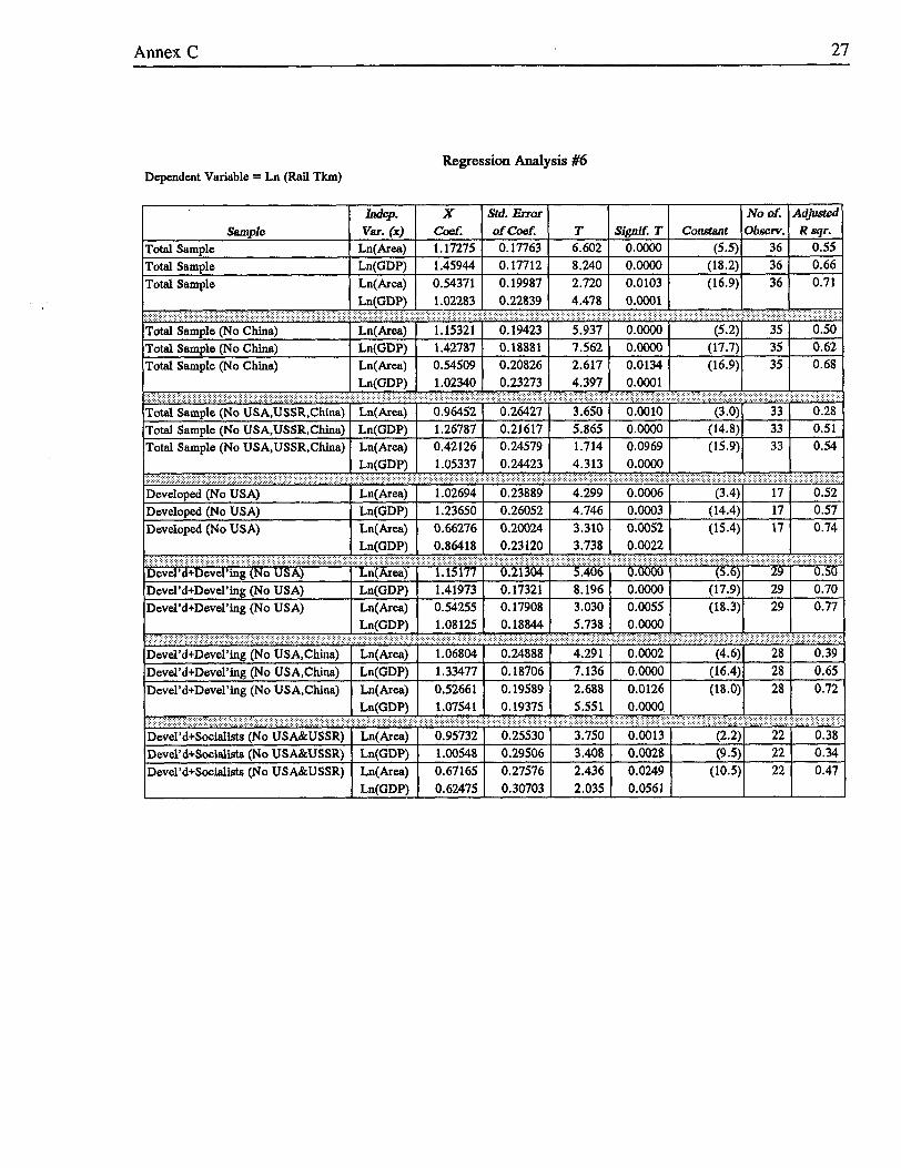
Dependent Variable = Ln (Rail Tkm) Regression Analysis #6

1 Indep. 1 X ISrd.EnorI I I

1 Ln(GDP) 1 1.02283 1 0.22839 1 4.478 1 O.OOOl l I I ,.. ,:.:.::: ..,, ..:.,.:.:.:.:., .,.:.:.:.::~~ .,.:.,: .,..,. :.. . . . . . . . . ...’ ::,;:;,;.i:, ,.::.:::.,. .,.,.: .,.........: .:.:.:.:.:. ,., ,. .,., ,.... ..:: . . . . . . . . .,.,: :::::; . . . . . :.:.:..::. : ..,.. ,.,.,., ;.... . . . . . . . . . :.:.:j:j::. ,.. >..:.:.::: . . . . ..:.::.:.:.:.>:.: ..::.:.:.:.: . . . . . . . ~:::: . ,.... ..,. ./...... . . . . . . . . . . . . . . . . . . . . . . . . . . ..A .,iii:i;l:,: ., ::;;;;y;: ..,I:, jjj;:::: j I,., :::<:; :I,, :::,:; 5.937 o.o&o

‘.‘.‘. . . . . . .,.,.,... :. .,..., .‘. .: . . ..:.> . . . . . :.:.: . . . . . :.:.:.::::::~:~::::::::~:~~:,j:. . .:..., ,.,..............,.. ,.,.<;j:j:j:l::<:~, __yI1I_I__L__c_LyLc_ Total Sample (No China) Ln(Area) (5.2) 35 0.50 Total Sample (No China) Ln( GDP) 1.42787 0.18881 7.562 O.OOOO (17.7) 35 0.62 Total Sample (No China) Ln(Area) 0.54509 0.20826 2.617 0.0134 (16.9) 35 0.68

1 Ln(GDP) 1 1.02340 I 0.23273 1 4.397 1 O.OOOl ) .:::.::;::::::::::::.:... ‘.‘:‘:‘:‘:‘. :..:.:x:::::: :‘:‘:x:::::::::: :.:::::::,:..: .“““’ .‘.:........‘.‘.. .)):.:.~:...:...:.:.. . . . . . . . . . . . . . . . . : ,.,.,:,:,..,: .:.::::::j: ..:::.;j :....,.....,, >y.: .//,. :::;i:::,::;:.,j: .;.jii:jj,jj:jj:::, ,“,:::,:,;:;:;: ,. .:::.$:;$:;,: :::;;;;;:I:l, ,. . . . . . . .j:i:j:iiiiillll:llli:ii::iiiiilllii:.: ‘, i;$$i:y.~ :,;:;;;;;::,: : ‘:i;;;l:, .::: i:::;:;;l:l.l :,jj:j:::::.. ,:j::::,:,. :,: :::::::j: :.,, ;j:,j:j::,, ! ., . . ., ., ., ., . . . . 1, : :.:::.. .,. .,., .,., ,..i_,::::III:j:j:::::: . . . . . . . . . . . . . . . . . . . . . . . . . . . . . . . . . :.,,.,:,:,;.;, ,. . ...:.:...>,. ./ . . . . . . . :\, . . . . . . . ., Total Sam ,ule (No USA.USSR.China\ 1 Lnkeal 1 0.96452 1 o.2@ 127 1 3.650 1’ 0.0010 1 (3.0)1 33 1 0.28

5.865 I o.oooo I h4.8;1 33 1 0.511 Total Sample (No USA,USSR,China) 1 Ln(GDP) 1 1.26787 1 0.21617 I Total Sample (No USA,USSR,China) 1 Ln(Area) 1 0.42126 1 0.24579 ( 1.714 I 0.0969 i15.9jj 33 ( 0.54

0.244231 o.oooo~ .,.,...,...,.jjj,......., : :, :, :, ,. . . . . . . . . . . . . .:i. . . . . ..A .,.. :.,: :..,:...: ;: . . . . . . ::;‘;I I:::::::::.~:.:.::::.::.....‘.‘::~~:.~::::~::::::~ ,,,,, .,.,:,, ,. .,:,,: ,.,., :..:.:.: .,,.,., ,., :. . . . . . . .

0.23889 1 4.299 ) O.OOO6 1 (3.4)1 17 1 0.52 0.26052 1 4.746 1 O.OOO3 1 (14.411 17 I 0.57

Devel’d+Devel’ing (No USA)

. . . . . . . ..‘.‘.‘..‘...‘.‘.........:.:.:.:.:.:.:.:.:...:...: ,.:...: . . . . :.‘.’ . . . . . . . . . . :. . . . . . . . . . . . . . . . . .) ,.,. . . . . . . :. .:.,. . . . . . . . . . . . :,::. . . . . ..c .,. .,. . . . . . . . :::::j; ,,,., ,, ,::::::.+..:::: . . . :.:::,:: ,.p..j: :::::,.::,.:::.....:...:.~:.::.:.:.: .,:; :,, :,.,:.; ::::::.::jj~:::.:.,.:j:.~.: ::::::... ,.,: :.:.:.: ., .P.... .A. . .y:,::... . ...: :.:.::::::):::.....:::.:.,. ..:.:::.,.:.:...:.:::.,.::: . . . . . . . .,.: :,.,. v:: :.:.::)::::::::::::.~:~:~:~:::::y :.))::)::::.j:::::j:::j): 3::::::. . ..:::.,. Devel’d+Socialists (No USA&USSR) Ln(Area) 0.95732 0.25530 3.750 o.oo13 (2.2) 22 0.38 Devel’d+Sccialists (No USA&USSR) Ln(GDP) 1 .OO548 0.29506 3.408 0.0028 (9.5) 22 0.34 Devel’d+Socialists (No USA&USSR) Ln(Area) 0.67165 0.27576 2.436 0.0249 (10.5) 22 0.47

I Ln(GDP) I 0.62475 I 0.30703 I 2.035 I 0.0561 I I J

Annex C

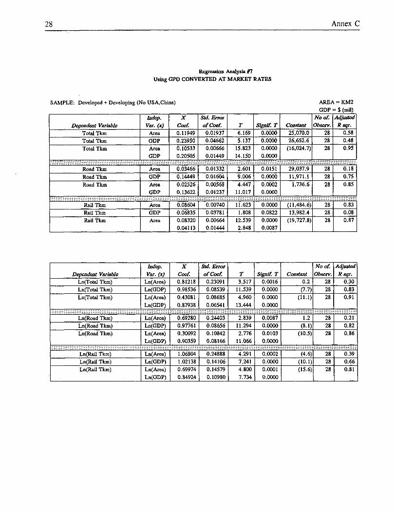
Regredon Aaalysie #I Using GPD CONVERTED AT MARKET RATES

SAMPLE: Developed + Developing (No USA,China) AREA = KM2 GDP = $ (mil)

Rail Tkm Area 0.08320 0.00664 12.539 0.0000 (19,727.a) 28 0.87 0.04113 0.01444 2.848 0.0087

X IStd.Error( I I No of.

TEST FOR EQUALITY OF CQEFFICIEN’IS

1. Sum of Squared Residuals

DEPENDENT VARIABLE

2. The Test Statistic

F* = [(SSRd” - SSRd - SSRJk] / [(.%Rd + SSRtJ/(nd + nu - 2k)]

where: d = developed u = developing or socialist n = number of observations k = number of parameters

3. Value of F*, and critical values (Fe) for the F distribution at the 0.05 point.

Total Road Rail Ln(Total) Ln(Road) In(Rai1) Dev’d + Dev’g: F* = 4.563 1.568 1.994 2.968 3.886 1.220

Dev’d + Socialist: F* = 7.374 0.021 7.684 7.297 1.456 8.156

Critical Values Dev’d + De@ Fc3.22 = 3.05 Dev’d + So&hit: Fc3,16 = 3.24

WPS977

Title

income Security for Old Age: Conceptual Background and Major

WPS978 How Restricting Carbon Dioxide Charles R. Biitzer and Methane Emissions Would Affect R. S. Eckaus the Indian Economy

WPS979 Economic Growth and the Environment

WPS980 The Environment: A New Challenge for GATT

WPS981 After Socialism and Dirigisme: Which Way?

WPS982 Microeconomics of Transformation in Poland: A Survey of State Enterprise Responses

WPS983 Legal Reform for Hungary’s Private Sector

WPS984 Barriers to Portfolio Investments in Emerging Stock Markets

WPS985 Regional integration, Old and New

WPS986 The Administration of Road User Taxes in Developing Countries

WPS987 How the Epidemiological Transition Affects Health Policy issues in Three Latin American Countries

WPS988 Economic Valuation and the Natural World

WPS989 The Indian Trade Regime

WPS990

WPS991

Protection and industrial Structure in India

Environmental Costs of Natural Resource Commodities: Magnitude and incidence

Policy Research Working Paper

Author

Esteiie James

Supriya Lahiri Alexander Meeraus

Dennis Anderson

Piritta Sorsa

And&s Solimano

Brian Pinto Marek Belka Stefan Krajewski

Cheryl W. Gray Rebecca J. Hanson Michael Heller

Asli Demirgiig-Kunt Harry Huizinga

Jaime de Melo Claudio Montenegro Arvind Panagariya

Roy Bahl

Jose Luis Bobadilla Cristina de A. Possas

David Pearce

M. Ataman Aksoy

M. Ataman Aksoy Francois M. Ettori

Margaret E. Slade

Date

September 1992

September 1992

September 1992

September 1992

September 1992

September 1992

Gctober 1992

October 1992

October 1992

October 1992

October 1992

October 1992

October 1992

October 1992

October 1992

Contact for paper

i3. Evans 37489

WDR Gffice 31393

WDR Office 31393

WDR Gffice 31393

S. Fallon 37947

S. Husain 37139

R. Martin 39065

W. Patrawimolpon 37664

D. Baliantyne 37947

J. Francis-O’Connor 35205

0. Nadora 31091

WDR Gffice 31393

R. Matenda 35055

R. Matenda 35055

WDR Office 31393

Policy Research Working Paper Series

Title Author Date

WPS992 Regional integration in Sub-Saharan Faezeh Foroutan Africa: Experience and Prospects

October 1992

WPS993 An Economic Analysis of Capital S. Ibi Ajayi October 1992 ~Flight from Nigeria

MIPS994 Textiles and Apparel in NAFTA: Geoffrey Bannister October 1992 A Case of Constrained Liberalization Patrick Low

WPS995 Recent Experience with Commercial Stijn Claessens October 1992 Bank Debt Reduction lshac Diwan

Eduardo Fernandez-Arias

WPS996 Strategic Management of Population Michael H. Bernhart October 1992 Programs

WPS997 How Financial Liberalization in John R. Harris October 1992 Indonesia Affected Firms’ Capital Fabio Schiantarelli Structure and Investment Decisions Miranda G. Siregar

WPS998 What Determines Demand for Freight Esra Bennathan October 1992 Transport? Julie Fraser

Louis S. Thompson

Contact for paper

S. Fallon 37947

0. Miranda 34877

A. Daruwala 33713

Rose Vo 33722

0. Nadora 31091

W. Pitayatonakarn 37664

8. Gregory 33744