what do cooperative firms maximize, if at all? evidence
TRANSCRIPT
ISSN 2282-6483
What Do Cooperative Firms
Maximize, if at All?
Evidence from Emilia-Romagna
in the pre-Covid Decade
Guido Caselli Michele Costa
Flavio Delbono
Quaderni - Working Paper DSE N°1159
1
What Do Cooperative Firms Maximize, if at All?
Evidence from Emilia-Romagna in the pre-Covid Decade°
Guido Casellia, Michele Costab and Flavio Delbonob
a Unioncamere Emilia-Romagna, V.le A. Moro 62, 40127 Bologna, Italy
b Department of Economics, University of Bologna, P.za Scaravilli 2, 40126 Bologna, Italy
([email protected]; [email protected], corresponding author)
Abstract
The Italian region Emilia-Romagna ranks first among the world’s most important cooperative
districts. Using a unique dataset covering all firms registered in the region, we investigate the
performance of active firms in the period 2010-18. By focusing on employment, revenue and profits
of cooperative firms as compared to conventional firms, we disentangle the differences between the
average performance of the two types of companies and detect the presence of a “size effect”
driving much of the difference between them. Moreover, our results strengthen previous empirical
evidence about the countercyclical role of cooperative firms: they seem to optimize a mixture of
employment and profits, assigning a greater weight to the former during downturns and stagnation.
Finally, we examine the regional logistics industry and compare also the profitability of employees
in the two segments of the sector.
JEL Codes: L21, L25
Keywords: cooperative firms, employment, Gini decomposition
° We thank Daniele Brusha, Stefano Zamagni and Vera Zamagni for help and suggestions. The
usual disclaimer applies.
2
Non-Technical Summary
Given the importance of the cooperative movement in the Italian economy, and in particular in the
Emilia-Romagna region, we utilize the unique dataset of the regional Chamber of Commerce to
compare the cooperative firms and the conventional ones. In investigating the balance sheets of all
firms registered in the region between 2010 and 2018, we concentrate on employment, revenues and
profits. We show that the main differences between the two types mostly occur within the large
firms (in terms of revenue). Moreover, our research confirms that the cooperative companies
(including stock companies controlled by cooperatives) care more about employment than profits
and their actions contribute to stabilize employment, especially during downturns. Finally, we
deepen the performance of the regional logistics industry and underline some remarkable difference
between cooperative and noncooperative firms. Hence, contrarily to the behavior assumed in a
consolidated theoretical literature, in reality cooperative firms seem to optimize a blend of
employment and profits, adjusting pay and sacrificing profits when needed to protect employees.
3
1. Introduction
An apparent lasting issue in comparative economics deals with the differences between cooperative
firms (sometimes labelled labour-managed firms, LMF)1 and conventional, i.e, non-cooperative
firms (NCFs, hereafter). To tackle this issue, theory is of little help. The overcited approach
pioneered by Ward (1958) and retained by his epigones, is patently inadequate. His formulation,
according to which a workers’ firm2 would maximize added value, net of non-labour costs per
member, raises two severe objections. On the theoretical grounds, in a competitive economy - as
well as under monopoly, as shown in Gal-or et al. (1980) - such formulation entails the annoying
negative relationship between output price shock and output response3. Moreover, such approach
finds no empirical support.
However, one may arguably disregard such extreme and unlikely market structures. In reality, CFs
operate in oligopolistic markets4; more precisely, in mixed oligopolies, i.e., concentrated industries
hosting companies pursuing different goals (see De Fraja and Delbono, 1990). Unfortunately, again,
theoretical models do not provide significant insights about the “correct” maximand of cooperative
firms, nor for the properties of the equilibria resulting from market interaction with profit-
maximizing companies (see, for instance, Craig and Pencavel 1993, Perotin 2006 and the literature
cited in Delbono and Reggiani 2013).
As for the objective function, an interesting route is explored by Kahana and Nitzan (1989).5 Under
price-taking behaviour, a workers’ firm (in which labour force coincides with membership), selects
inputs and output to maximize (i) income per worker/member subject to an employment constraint
or, alternatively, (ii) employment subject to a profit per worker/member constraint (bounded below
1 We do prefer “cooperative firms” because such a category encompasses various types of companies,
including cooperatives that are not owned and/or run by workers.
2 A worker’s firm is one in which all workers are members and all members are workers: Sertel (1982).
3 This is the well-known perverse effect, and it is not the only one. As shown in Delbono and Lambertini
(2014), in an oligopolistic supergame among Ward-like firms, in equilibrium tacit collusion is increasing in
the number of participants, as opposed to the standard conclusion with profit-maximizing players.
4 A notable exception is provided by some markets for childcare services, disadvantaged people, elderly:
here buyers are often local public institutions auctioning the provision of such services to groups of social
cooperatives (much active in Italy since the early ‘90s of the last century). Such markets often fit the form of
oligopsony.
5 For clarity, the route explored by Kahana and Nitzan (1989) goes back to Law (1977) who considers an
augmented utility function of LMFs’ members to include the membership size in addition to income. Law’s
paper, in turn, was inspired by Fellner (1947).
4
by the union wage). Standard duality arguments show the equivalence between (i) and (ii), both
formulations trying to capture the concern for employment that should shape the behaviour of firms
owned and controlled by workers-members. Of course, for a given number of workers, an LMF
becomes indistinguishable from a profit-maximizer. We shall come back to the relevance of this
approach in the conclusions. Here it suffices to note that the comparative statics by Kahana and
Nitzan (1989) may avoid perverse effects, depending on whether labour is a normal input.6
Hence, being the theory inconclusive and/or unfit to stylize actual markets, one is forced to resort to
empirical investigation. This paper provides a simple descriptive statistical analysis to contribute to
such still tiny stream of research and to have an insight about the underlying behavioural premises
driving the choices of cooperative firms. We try to infer their implicit objective function from
observed behaviour as measured by their performance.
Our benchmark is provided by the Italian region Emilia-Romagna (ER, hereafter) in the period
between the great recession of 2009 and the dramatic downturn fuelled by the pandemics in 2020.
Moreover, the regional setting allows one to detect the aggregate effect of the overall cooperative
magnitude. With this, we mean the set of: (i) cooperative firms; (ii) NCFs controlled by cooperative
firms; (iii) consortia of cooperative companies; (iv) cooperative associations. While the weights of
(iii) and (iv) are negligible in terms of number of employees - our rough estimate amounts to about
500 white collars altogether - and revenues, the size of (ii) is highly significant, especially in the
insurance, banking and facility management industries and cannot be ignored. Hence, by now, CFs
will mnemonics for both (i) and (ii), provided that we will specify if we refer to (i) or (ii) when
needed.
Our main findings can be summarized as follows:
• CFs and NCFs are very different in average size, particularly when looking at the subset of
firms above the median revenue7, in terms of employment, revenue and profits.
• Employment and revenues are much more countercyclical in CFs than in NCFs.
• CFs “profits”8, especially in recessions and stagnating periods, are pressed and employment
levels are stabilized or increased.
6 If this is the case, the supply function of an LMF is positively sloped; Kahana and Nitzan (1980), p. 537.
7 We choose operating revenue (or revenue from sales) as a comparable variable between both types of firms
instead of the so-called “value of production” recorded in production CFs’s balance sheets because it has no
clear counterpart in NCFs.
8 We postpone to Section 3 a discussion on the interpretation of “profits” in CFs.
5
• CFs seem to optimize9 their employment levels under a non-negative profit constraint (or
profits under an employment constraint).
• The industry case study of logistics strengthens the above conclusions hinting at a
remarkable difference in labour productivity between CFs and NCFs.
The empirical literature mostly related to our contribution includes a group of papers testing and
confirming that cooperative firms tend to act countercyclically as for their employment decisions
and that no perverse effect seems to emerge as a reaction to output demand shocks. These
conclusions have been validated, for instance, by: Burdin and Dean (2009, 2012) for some
Uruguay’s industries; Craig and Pencavel (1992, 1995) for the plywood industry of the US Pacific
Northwest; Delbono and Reggiani (2013) for production cooperatives in the Italian economy
immediately after the 2008 financial crisis; Navarra (2016) for a sample of Italian cooperatives
between 2000 and 2005. All these papers detect an employment stabilizing effect of cooperatives’
behaviour. While NCFs tend to adjust employment relatively to fluctuations in demand, production
cooperatives adjust pay to protect workplaces, at least towards their members (see Perotin 2012 for
a disquisition on the subject).
This paper is organized as follows. In Section 2 we sketch the Emilia-Romagna economy in the
period 2010-18, describe the dataset and illustrate our sample. Section 3 focuses on a comparative
analysis of cooperative firms wrt to conventional firms in terms of employment, revenue and
profits. In Section 4 we divide our sample in two groups depending on the revenue being above or
below the median and proceed to compare the relative performance of CFs vs NCFs. Section 5
examines an industry case study by briefly replicating the aforementioned analysis for the regional
logistics sector. Here we also deal with the apparently huge handicap of CFs wrt NCFs in terms of
labour productivity. Section 6 concludes.
1. The dataset and sample
As measured by the impact of CFs on employment and GDP, Italy ranks top in Western countries
and ER comes first among the Italian regions.10 Hence, ER represents a fairly sound environment to
examine the relative performance of CFs versus NCFs, as well as the differences within CFs.
9 We do prefer this word to maximize, as the latter refers to a standard conceptual frame which unfits the
variety of organizations belonging to our set of CFs.

6
It is worth emphasizing that modern cooperatives differ significantly from Sertel’s ideal type of
workers’ cooperative often assumed in the theoretical literature. Indeed, the so-called membership
ratio (number of members over the number of employees) is lower than one, especially in the
biggest CFs. Unfortunately, the value of such ratio is absent in the balance sheets and it is only
occasionally made public through reports of CFs associations at the aggregate (industrial and/or
territorial) level. However, to envisage an order of magnitude, in a large sample of Italian
production CFs part of Legacoop, the membership ratio was roughly 0.7 around approximately ten
years ago (Delbono and Reggiani, 2013).
The source of our dataset is the ER Chamber of Commerce which collects the balance sheets of all
companies registered in its regional database. Specifically, we focus on the 2010-2018 time set
because this period has the most accurate dataset and comes after the deep downturn following the
2008 financial crisis. The following table summarizes the regional GDP and the employee trends
compared to the national ones.
Table 1. GDP (at market prices, million euros, linked values, basis 2015) and employees, ER and
Italy (source, Istat)
When inspecting this database, one must give attention to the geographical interpretation of figures
about employment. Both CFs and NCFs registered in ER – especially the largest ones – employ
10 See, for instance, Navarra (2016), International Co-operative Alliance (2017), Zamagni (2019) and Euricse
(2020). The cooperative movement in Italy evolved around three main associations (Legacoop,
Confcooperative and Agci, now coordinating their actions under the label ACI) including the vast majority
of sizeable cooperative organizations in terms of revenue and employment. In 2017, 60% of cooperative
firms registered in ER adhere to an association, accounting for almost 90% of overall cooperative
employment (Regione Emilia-Romagna, 2019).
GDP Employment
Year ER Italy ER Italy
2010 148.361 1.711.622 1.906.496 22.526.851
2011 152.278 1.723.612 1.934.279 22.598.244
2012 147.925 1.672.284 1.927.925 22.565.972
2013 146.834 1.641.333 1.904.093 22.190.535
2014 148.316 1.641.346 1.911.463 22.278.918
2015 149.111 1.654.204 1.918.318 22.464.753
2016 151.636 1.675.210 1.967.141 22.757.840
2017 155.147 1.703.002 1.973.043 23.022.958
2018 157.870 1.716.622 2.004.879 23.214.951
7
labour force also outside the regional boundaries (from here on, employees); on the other hand, in
the regional area we observe employees of CFs and NCFs registered in other regions (local
production unit employees). In this paper we will focus on the employees. This means that we shall
emphasize the economic consequences of decisions taken in the corporate headquarters located in
ER, being obviously aware that they happen also elsewhere. First of all, we partition the total
number of firms registered in ER into the two groups.
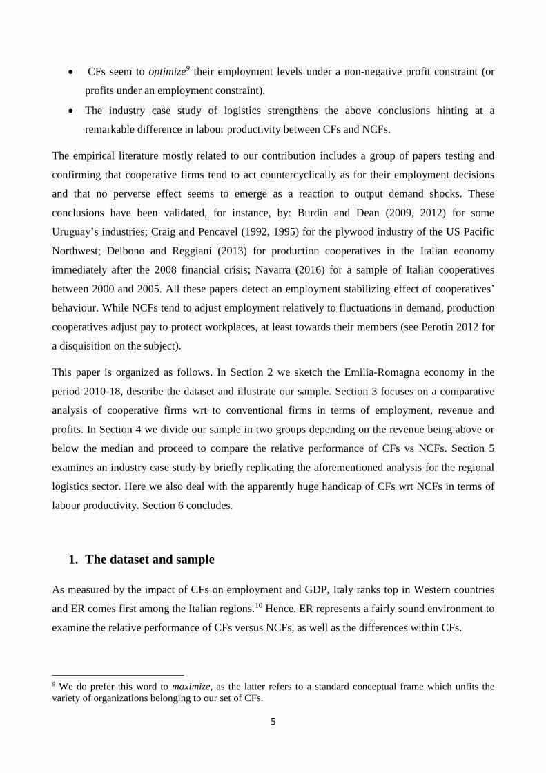
Table 2. Number of CFs and NCFs registered in ER
NCF CF TOTAL
2010 68.127 4.475 72.602
2011 68.979 4.411 73.390
2012 68.193 4.351 72.544
2013 67.889 4.290 72.179
2014 68.141 4.252 72.393
2015 68.762 4.176 72.938
2016 69.960 4.093 74.053
2017 70.656 3.983 74.639
2018 70.750 3.798 74.548
While we start considering the entire set of firms registered in the Chambers of Commerce of ER,
our intention is to focus on a sample composed only by those actually active firms. Therefore, we
exclude all companies – both CF and NCF – that did not submit their balance sheets and/or that do
not have employees at all.
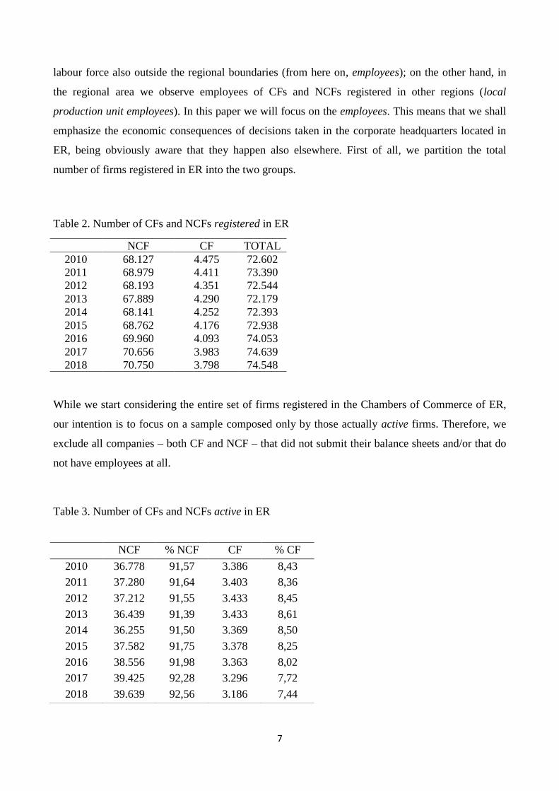
Table 3. Number of CFs and NCFs active in ER
NCF % NCF CF % CF
2010 36.778 91,57 3.386 8,43
2011 37.280 91,64 3.403 8,36
2012 37.212 91,55 3.433 8,45
2013 36.439 91,39 3.433 8,61
2014 36.255 91,50 3.369 8,50
2015 37.582 91,75 3.378 8,25
2016 38.556 91,98 3.363 8,02
2017 39.425 92,28 3.296 7,72
2018 39.639 92,56 3.186 7,44
8
Table 3 summarizes the composition of the resulting sample: having our dataset been cleared from
inactive firms, its size considerably shrinks.
Moreover, due to entries and exits, the list of active firms varies over time: restricting the attention
solely to persistently active firms over the entire time span would reduce the sample even more.
To provide an insight on the economic relevance of both types of firms in the regional system, we
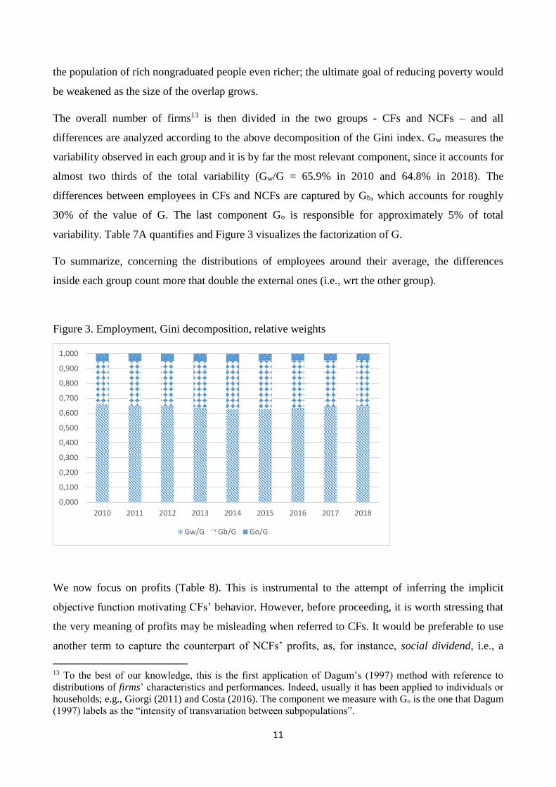
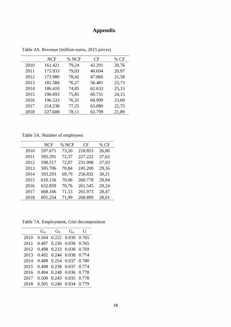
summarize their revenues in Table 4A11 and plot them in Figure 1.
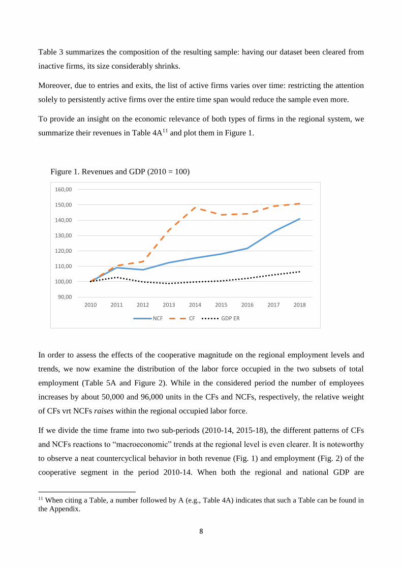
Figure 1. Revenues and GDP (2010 = 100)
In order to assess the effects of the cooperative magnitude on the regional employment levels and
trends, we now examine the distribution of the labor force occupied in the two subsets of total
employment (Table 5A and Figure 2). While in the considered period the number of employees
increases by about 50,000 and 96,000 units in the CFs and NCFs, respectively, the relative weight
of CFs vrt NCFs raises within the regional occupied labor force.
If we divide the time frame into two sub-periods (2010-14, 2015-18), the different patterns of CFs
and NCFs reactions to “macroeconomic” trends at the regional level is even clearer. It is noteworthy
to observe a neat countercyclical behavior in both revenue (Fig. 1) and employment (Fig. 2) of the
cooperative segment in the period 2010-14. When both the regional and national GDP are
11 When citing a Table, a number followed by A (e.g., Table 4A) indicates that such a Table can be found in
the Appendix.
90,00
100,00
110,00
120,00
130,00
140,00
150,00
160,00
2010 2011 2012 2013 2014 2015 2016 2017 2018
NCF CF GDP ER
9
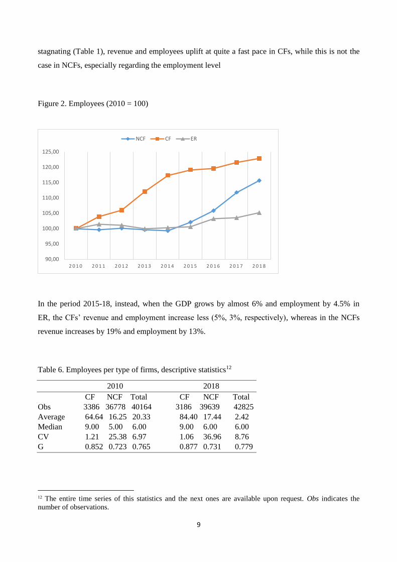
stagnating (Table 1), revenue and employees uplift at quite a fast pace in CFs, while this is not the
case in NCFs, especially regarding the employment level
Figure 2. Employees (2010 = 100)
In the period 2015-18, instead, when the GDP grows by almost 6% and employment by 4.5% in
ER, the CFs’ revenue and employment increase less (5%, 3%, respectively), whereas in the NCFs
revenue increases by 19% and employment by 13%.
Table 6. Employees per type of firms, descriptive statistics12
2010 2018
CF NCF Total CF NCF Total
Obs 3386 36778 40164 3186 39639 42825
Average 64.64 16.25 20.33 84.40 17.44 2.42
Median 9.00 5.00 6.00 9.00 6.00 6.00
CV 1.21 25.38 6.97 1.06 36.96 8.76
G 0.852 0.723 0.765 0.877 0.731 0.779
12 The entire time series of this statistics and the next ones are available upon request. Obs indicates the
number of observations.
90,00
95,00
100,00
105,00
110,00
115,00
120,00
125,00
2 0 1 0 2 0 1 1 2 0 1 2 2 0 1 3 2 0 1 4 2 0 1 5 2 0 1 6 2 0 1 7 2 0 1 8
NCF CF ER
10
Other substantial differences emerge among CF and NCF (Tables 5A and 6). Considering, for
instance, the last year of our interval, while representing less that 8% of the sample, CFs account for
over 28% of total employment. Incidentally, this confirms that the presence of CFs is biased
towards labor-intensive industries.
Besides being greater than NCFs in terms of average number of employees, CFs also differ
regarding the overall distribution of labor force around their average size (Table 6). This is self-
evident from the values of the Coefficient of Variation (CV), the difference between average and
median and the value of the Gini index (G). These features underline the presence of a heavy right
tail and a strong positive skewness in the distribution of employment across CFs. This is another
reason why it is not advisable to use the average as a proxy of the distribution, or any other
econometric tool based on it, as, for instance, the OLS.
2. CFs vs NCFs: employment, revenues and profits
To elaborate on the differences between the two distributions of employees in both types of firms,
we decompose the Gini index by following the approach pioneered by Dagum (1997). Accordingly,
the differences among all pairs of values embedded in the Gini formula are subdivided into three
components: inequality within the group (Gw); inequality between the groups (Gb) and the
overlapping factor (Go).
The overlapping factor represents an important, and often neglected aspect in the analyses of the
key factors driving inequalities in statistical distributions. To clarify its relevance - if not too
pedagogically - suppose that all CFs are “large” (wrt to some dimension), whereas all NCFs are
“small”. Here their size is fully explained by the nature of the company. In the opposite scenario,
suppose the distributions of the two groups of firms fully coincide; in this case, the size is not
explained at all by the company being CF or NCF. In reality, however, the distributions of two
groups - CFs and NCFs in our setting - usually overlap; hence, to continue our illustration, we will
observe also small CFs and large NCFs. Here is where Go kicks off, by measuring a portion of total
variability which is not captured by Gw nor by Gb. To add a potential policy implication of Dagum’s
approach, consider a setting in which all rich people are college graduate, and all poor people are
not. To reduce poverty, one may then tax the graduate ones. In presence of an overlap between the
two distributions, however, such a policy would result in making poor graduates even poorer and
11
the population of rich nongraduated people even richer; the ultimate goal of reducing poverty would
be weakened as the size of the overlap grows.
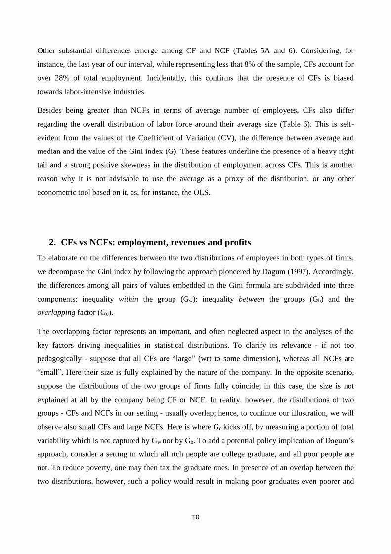
The overall number of firms13 is then divided in the two groups - CFs and NCFs – and all
differences are analyzed according to the above decomposition of the Gini index. Gw measures the
variability observed in each group and it is by far the most relevant component, since it accounts for
almost two thirds of the total variability (Gw/G = 65.9% in 2010 and 64.8% in 2018). The
differences between employees in CFs and NCFs are captured by Gb, which accounts for roughly
30% of the value of G. The last component Go is responsible for approximately 5% of total
variability. Table 7A quantifies and Figure 3 visualizes the factorization of G.
To summarize, concerning the distributions of employees around their average, the differences
inside each group count more that double the external ones (i.e., wrt the other group).
Figure 3. Employment, Gini decomposition, relative weights
We now focus on profits (Table 8). This is instrumental to the attempt of inferring the implicit
objective function motivating CFs’ behavior. However, before proceeding, it is worth stressing that
the very meaning of profits may be misleading when referred to CFs. It would be preferable to use
another term to capture the counterpart of NCFs’ profits, as, for instance, social dividend, i.e., a
13 To the best of our knowledge, this is the first application of Dagum’s (1997) method with reference to
distributions of firms’ characteristics and performances. Indeed, usually it has been applied to individuals or
households; e.g., Giorgi (2011) and Costa (2016). The component we measure with Go is the one that Dagum
(1997) labels as the “intensity of transvariation between subpopulations”.
0,000
0,100
0,200
0,300
0,400
0,500
0,600
0,700
0,800
0,900
1,000
2010 2011 2012 2013 2014 2015 2016 2017 2018
Gw/G Gb/G Go/G
12
residual to be computed differently from the procedure delivering profits in NCFs.14 Moreover, our
overall sample includes a large variety of CFs: workers’, producers’, users’, social, credit’s and so
on (see Zamagni and Zamagni 2011). Hence these different roles of members within their CFs may
entail differences in CFs’ ultimate goals. Furthermore, by CFs in this paper we mean also the joint
stock companies controlled by cooperative holdings which may maximize profits to be distributed
as dividends to the controlling cooperative firms. This withstanding, we conform to the prevailing
terminology, while recommending caution when comparing “profits” between CFs and NCFs as
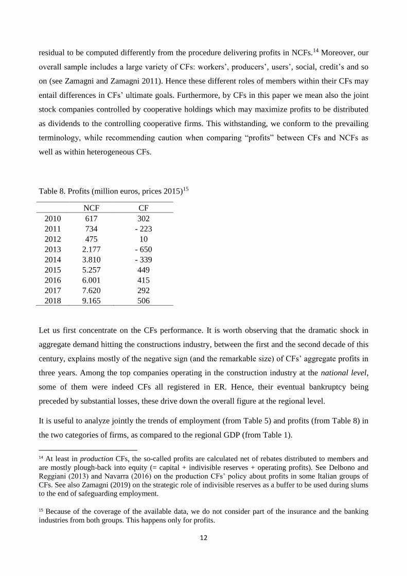
well as within heterogeneous CFs.
Table 8. Profits (million euros, prices 2015)15
NCF CF
2010 617 302
2011 734 - 223
2012 475 10
2013 2.177 - 650
2014 3.810 - 339
2015 5.257 449
2016 6.001 415
2017 7.620 292
2018 9.165 506
Let us first concentrate on the CFs performance. It is worth observing that the dramatic shock in
aggregate demand hitting the constructions industry, between the first and the second decade of this
century, explains mostly of the negative sign (and the remarkable size) of CFs’ aggregate profits in
three years. Among the top companies operating in the construction industry at the national level,
some of them were indeed CFs all registered in ER. Hence, their eventual bankruptcy being
preceded by substantial losses, these drive down the overall figure at the regional level.
It is useful to analyze jointly the trends of employment (from Table 5) and profits (from Table 8) in
the two categories of firms, as compared to the regional GDP (from Table 1).
14 At least in production CFs, the so-called profits are calculated net of rebates distributed to members and
are mostly plough-back into equity (= capital + indivisible reserves + operating profits). See Delbono and
Reggiani (2013) and Navarra (2016) on the production CFs’ policy about profits in some Italian groups of
CFs. See also Zamagni (2019) on the strategic role of indivisible reserves as a buffer to be used during slums
to the end of safeguarding employment.
15 Because of the coverage of the available data, we do not consider part of the insurance and the banking
industries from both groups. This happens only for profits.

13
Table 9. Profits, GDP and Employees (2010 = 100)
Profits GDP Employees
NCF CF ER NCF CF ER
2010 100,00 100,00 100,00 100,00 100,00 100
2011 119,05 -73,88 102,64 99,60 103,82 101,46
2012 76,98 3,36 99,71 100,14 106,01 101,12
2013 353,06 -215,25 98,97 99,67 112,04 99,87
2014 618,01 -112,23 99,97 99,27 117,35 100,26
2015 852,64 148,49 100,51 102,09 119,16 100,62
2016 973,38 137,45 102,21 105,89 119,51 103,18
2017 1236,06 96,72 104,57 111,79 121,53 103,49
2018 1486,56 167,29 106,41 115,66 122,87 105,16
Table 9 shows other striking differences between CFs and NCFs. For instance, let us consider the
interval 2010-14, a period of stagnation in which the Italian GDP falls by over 4% (Table 1) and the
regional one is experiencing a zero growth. As for the NCF, while their revenue increases by about
15% and their profits grows six-fold, their employment level slightly decreases. In contrast, the
CFs’ revenue goes up by 48%, profits decrease by 21.2% and, above all, employment raises by
more than 17%. In the 2015-18 timeframe, when the regional GDP is growing at an average rate of
1.5% per year, the revenue and employment levels of CFs grow slower (5% and 3%, respectively,
in 4 years) and their profits increase by 13%. The NCFs, instead, uplift their revenue by 19%,
profits by 74% and employment by 13%.
In the entire time span, while the regional GDP is at a standstill averaging a rate of about 0.65% per
year, the performances of CFs and NCFs are very different, especially as for the way in which
employment and profits accompany the course of their revenues. The latter increases by 41% for the
NCFs and by slightly more (48%) for the CFs. However, such a similar expansion in revenue yields
drastically diverging consequences: profits grow fourteenfold in CNF and only 67% in CFs,
whereas the number of employees increase by less than 16% in NCF and almost by 23% in CFs.
Here is one of the major findings of our statistical investigation. We have indeed registered a
remarkable difference in the reaction to demand shocks hitting both the local and national economy.
While (basically profit-maximizing) NCFs tend to be procyclical, CFs tend to stabilize their
employment and, given their critical mass, they contribute to flatter also the overall regional
employment level, at the cost of profits.
To obtain a quantitative summary of the relationships among revenues (RV), profits (PR) and
employment (EM) within the two group of firms, we calculate the correlation for all relevant pairs.
The next three tables collect the value of the correlation coefficient for the entire sample (Table 10),
14
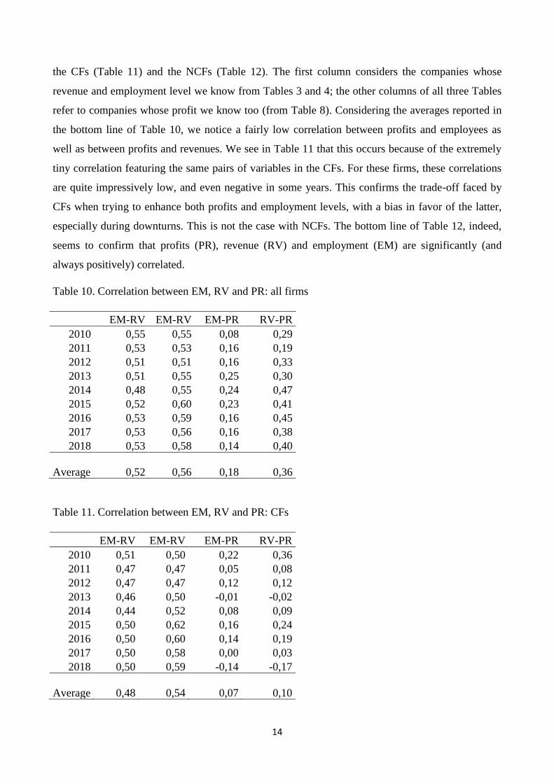
the CFs (Table 11) and the NCFs (Table 12). The first column considers the companies whose
revenue and employment level we know from Tables 3 and 4; the other columns of all three Tables
refer to companies whose profit we know too (from Table 8). Considering the averages reported in
the bottom line of Table 10, we notice a fairly low correlation between profits and employees as
well as between profits and revenues. We see in Table 11 that this occurs because of the extremely
tiny correlation featuring the same pairs of variables in the CFs. For these firms, these correlations
are quite impressively low, and even negative in some years. This confirms the trade-off faced by
CFs when trying to enhance both profits and employment levels, with a bias in favor of the latter,
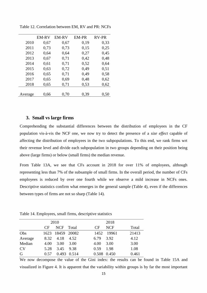
especially during downturns. This is not the case with NCFs. The bottom line of Table 12, indeed,
seems to confirm that profits (PR), revenue (RV) and employment (EM) are significantly (and
always positively) correlated.
Table 10. Correlation between EM, RV and PR: all firms
EM-RV EM-RV EM-PR RV-PR
2010 0,55 0,55 0,08 0,29
2011 0,53 0,53 0,16 0,19
2012 0,51 0,51 0,16 0,33
2013 0,51 0,55 0,25 0,30
2014 0,48 0,55 0,24 0,47
2015 0,52 0,60 0,23 0,41
2016 0,53 0,59 0,16 0,45
2017 0,53 0,56 0,16 0,38
2018 0,53 0,58 0,14 0,40
Average 0,52 0,56 0,18 0,36
Table 11. Correlation between EM, RV and PR: CFs
EM-RV EM-RV EM-PR RV-PR
2010 0,51 0,50 0,22 0,36
2011 0,47 0,47 0,05 0,08
2012 0,47 0,47 0,12 0,12
2013 0,46 0,50 -0,01 -0,02
2014 0,44 0,52 0,08 0,09
2015 0,50 0,62 0,16 0,24
2016 0,50 0,60 0,14 0,19
2017 0,50 0,58 0,00 0,03
2018 0,50 0,59 -0,14 -0,17
Average 0,48 0,54 0,07 0,10
15
Table 12. Correlation between EM, RV and PR: NCFs
EM-RV EM-RV EM-PR RV-PR
2010 0,67 0,67 0,19 0,33
2011 0,73 0,73 0,15 0,25
2012 0,64 0,64 0,27 0,45
2013 0,67 0,71 0,42 0,48
2014 0,61 0,71 0,52 0,64
2015 0,63 0,72 0,49 0,51
2016 0,65 0,71 0,49 0,58
2017 0,65 0,69 0,48 0,62
2018 0,65 0,71 0,53 0,62
Average 0,66 0,70 0,39 0,50
3. Small vs large firms
Comprehending the substantial differences between the distribution of employees in the CF
population vis-à-vis the NCF one, we now try to detect the presence of a size effect capable of
affecting the distribution of employees in the two subpopulations. To this end, we rank firms wrt
their revenue level and divide each subpopulation in two groups depending on their position being
above (large firms) or below (small firms) the median revenue.
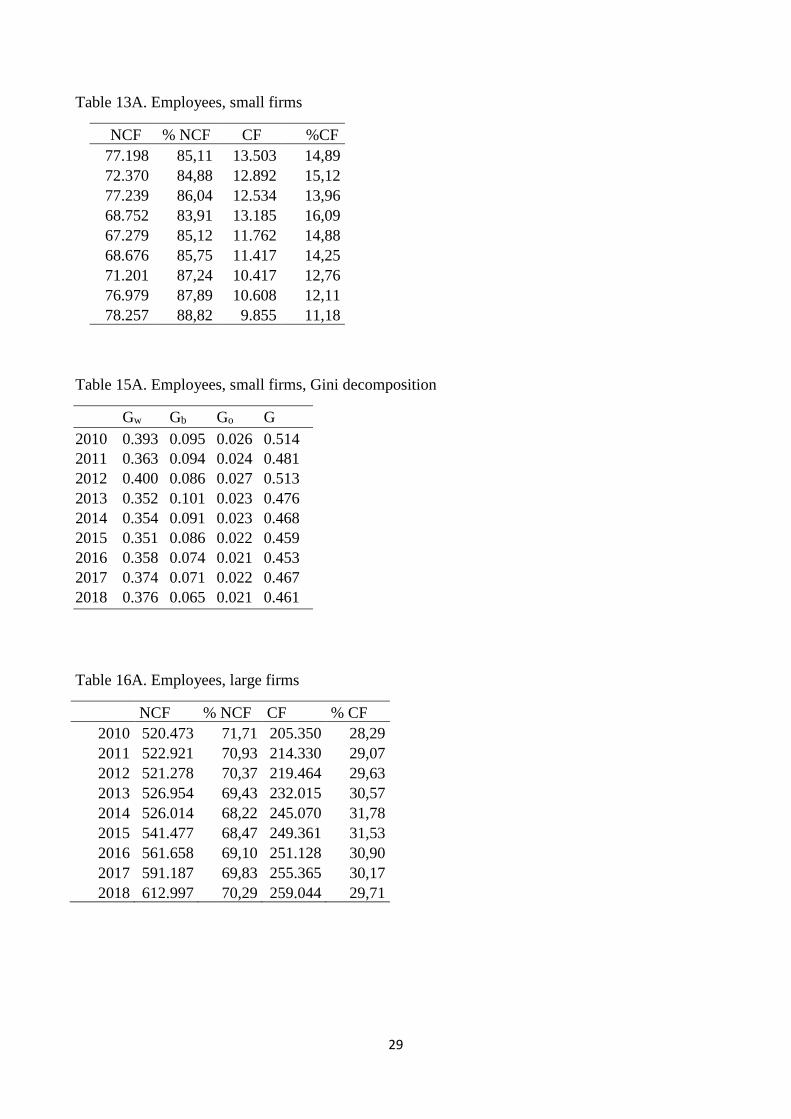
From Table 13A, we see that CFs account in 2018 for over 11% of employees, although
representing less than 7% of the subsample of small firms. In the overall period, the number of CFs
employees is reduced by over one fourth while we observe a mild increase in NCFs ones.
Descriptive statistics confirm what emerges in the general sample (Table 4), even if the differences
between types of firms are not so sharp (Table 14).
Table 14. Employees, small firms, descriptive statistics
2010 2018
CF NCF Total CF NCF Total
Obs 1623 18459 20082 1452 19961 21413
Average 8.32 4.18 4.52 6.79 3.92 4.12
Median 4.00 3.00 3.00 4.00 3.00 3.00
CV 5.28 3.45 9.38 0.59 1.98 1.08
G 0.57 0.493 0.514 0.508 0.450 0.461
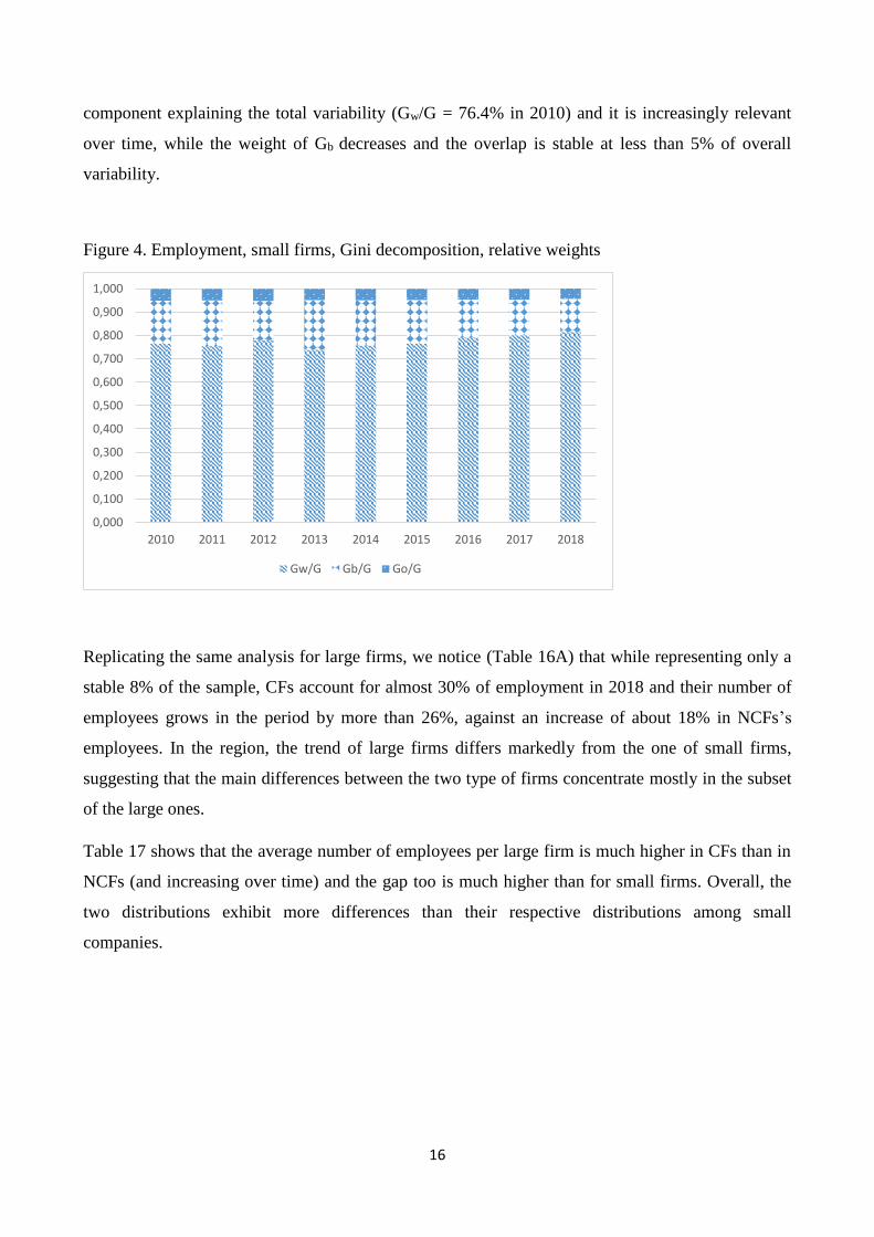
We now decompose the value of the Gini index: the results can be found in Table 15A and
visualized in Figure 4. It is apparent that the variability within groups is by far the most important
16
component explaining the total variability (Gw/G = 76.4% in 2010) and it is increasingly relevant
over time, while the weight of Gb decreases and the overlap is stable at less than 5% of overall
variability.
Figure 4. Employment, small firms, Gini decomposition, relative weights
Replicating the same analysis for large firms, we notice (Table 16A) that while representing only a
stable 8% of the sample, CFs account for almost 30% of employment in 2018 and their number of
employees grows in the period by more than 26%, against an increase of about 18% in NCFs’s
employees. In the region, the trend of large firms differs markedly from the one of small firms,
suggesting that the main differences between the two type of firms concentrate mostly in the subset
of the large ones.
Table 17 shows that the average number of employees per large firm is much higher in CFs than in
NCFs (and increasing over time) and the gap too is much higher than for small firms. Overall, the
two distributions exhibit more differences than their respective distributions among small
companies.
0,000
0,100
0,200
0,300
0,400
0,500
0,600
0,700
0,800
0,900
1,000
2010 2011 2012 2013 2014 2015 2016 2017 2018
Gw/G Gb/G Go/G
17
Table 17. Employees, large firms, descriptive statistics
2010 2018
CF NCF Total CF NCF Total
Obs 1763 18319 20082 1734 19678 21412
Average 116.48 28.41 36.14 149.39 31.15 40.73
Median 22.00 12.00 12.00 25.00 12.00 12.00
CV 0.86 19.94 5.39 0.84 27.88 6.79
G 0.819 0.671 0.725 0.843 0.681 0.741
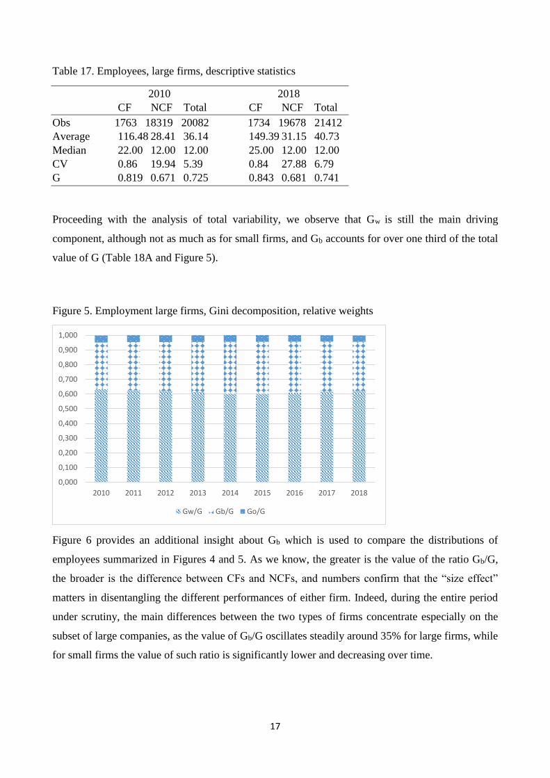
Proceeding with the analysis of total variability, we observe that Gw is still the main driving
component, although not as much as for small firms, and Gb accounts for over one third of the total
value of G (Table 18A and Figure 5).
Figure 5. Employment large firms, Gini decomposition, relative weights
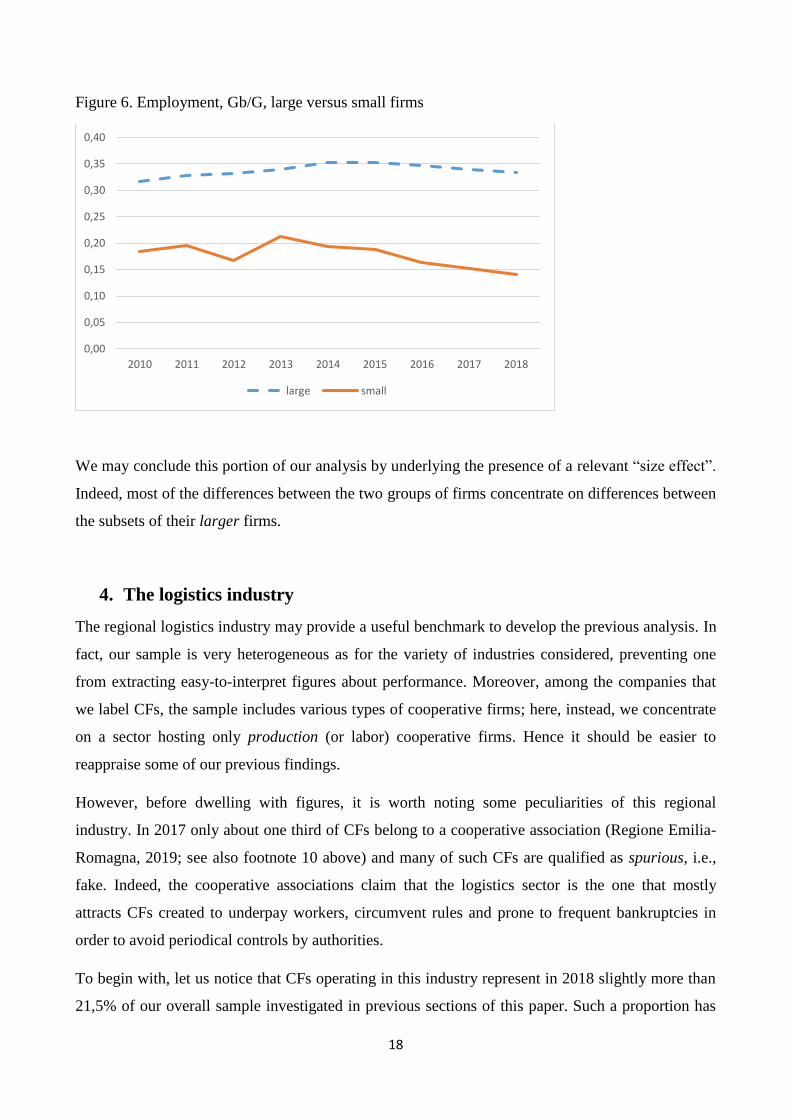
Figure 6 provides an additional insight about Gb which is used to compare the distributions of
employees summarized in Figures 4 and 5. As we know, the greater is the value of the ratio Gb/G,
the broader is the difference between CFs and NCFs, and numbers confirm that the “size effect”
matters in disentangling the different performances of either firm. Indeed, during the entire period
under scrutiny, the main differences between the two types of firms concentrate especially on the
subset of large companies, as the value of Gb/G oscillates steadily around 35% for large firms, while
for small firms the value of such ratio is significantly lower and decreasing over time.
0,000
0,100
0,200
0,300
0,400
0,500
0,600
0,700
0,800
0,900
1,000
2010 2011 2012 2013 2014 2015 2016 2017 2018
Gw/G Gb/G Go/G
18
Figure 6. Employment, Gb/G, large versus small firms
We may conclude this portion of our analysis by underlying the presence of a relevant “size effect”.
Indeed, most of the differences between the two groups of firms concentrate on differences between
the subsets of their larger firms.
4. The logistics industry
The regional logistics industry may provide a useful benchmark to develop the previous analysis. In
fact, our sample is very heterogeneous as for the variety of industries considered, preventing one
from extracting easy-to-interpret figures about performance. Moreover, among the companies that
we label CFs, the sample includes various types of cooperative firms; here, instead, we concentrate
on a sector hosting only production (or labor) cooperative firms. Hence it should be easier to
reappraise some of our previous findings.
However, before dwelling with figures, it is worth noting some peculiarities of this regional
industry. In 2017 only about one third of CFs belong to a cooperative association (Regione Emilia-
Romagna, 2019; see also footnote 10 above) and many of such CFs are qualified as spurious, i.e.,
fake. Indeed, the cooperative associations claim that the logistics sector is the one that mostly
attracts CFs created to underpay workers, circumvent rules and prone to frequent bankruptcies in
order to avoid periodical controls by authorities.
To begin with, let us notice that CFs operating in this industry represent in 2018 slightly more than
21,5% of our overall sample investigated in previous sections of this paper. Such a proportion has
0,00
0,05
0,10
0,15
0,20
0,25
0,30
0,35
0,40
2010 2011 2012 2013 2014 2015 2016 2017 2018
large small
19
been declining over time (27.8% in 2010), whereas the number of NCFs has been growing by over
17% in the same period.
Of course, the sample we are going to employ has been cleared as we did with the entire regional
sample. Tables 19A, 20A and 21A summarize, respectively, the number of firms, revenues and
employees, for both CFs and NCFs in the regional logistics industry. It emerges that employees are
almost split evenly between CFs and NCFs, although the former group is much less numerous than
the latter. This confirms that also in this highly labor-intensive sector, that CFs are larger than
NCFs, as summarized in Table 22.
Table 22. Employees, logistics, descriptive statistics
2010 2018
CF NCF Total CF NCF Total
Obs 452 1173 1625 377 1376 1753
Average 49.73 18.97 27.52 65.09 20.13 29.80
Median 17.00 6.00 8.00 18.00 7.00 8.00
CV 1.61 5.29 3.17 1.36 7.21 3.52
G 0.694 0.720 0.740 0.731 0.75 0.755
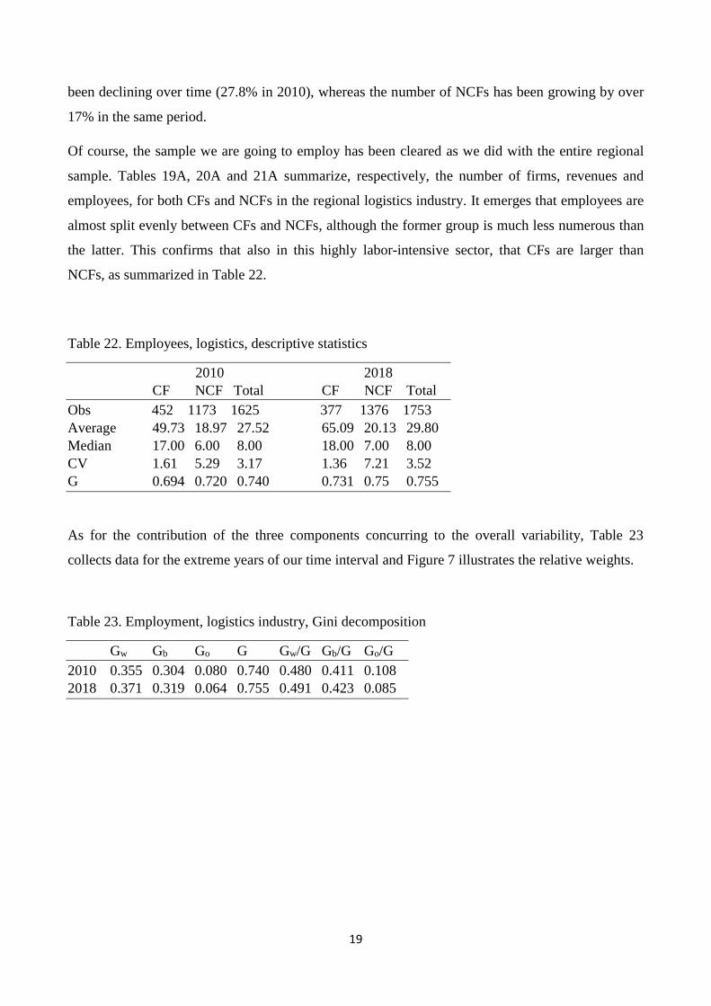
As for the contribution of the three components concurring to the overall variability, Table 23
collects data for the extreme years of our time interval and Figure 7 illustrates the relative weights.
Table 23. Employment, logistics industry, Gini decomposition
Gw Gb Go G Gw/G Gb/G Go/G
2010 0.355 0.304 0.080 0.740 0.480 0.411 0.108
2018 0.371 0.319 0.064 0.755 0.491 0.423 0.085
20
Figure 7. Employment, logistics, Gini decomposition, relative weights
It is interesting to remark that, as compared to the overall sample, in this case the variability within
(between) groups is much lower (higher); consequently, the type of company, more than the
differences within each type of distribution, matters greatly in explaining how employment differs
across companies. Moreover, the overlap factor is more significant than in the overall economy.
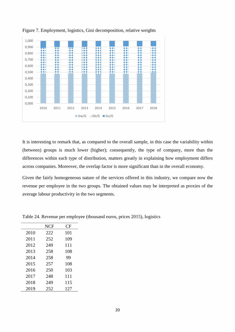
Given the fairly homogeneous nature of the services offered in this industry, we compare now the
revenue per employee in the two groups. The obtained values may be interpreted as proxies of the
average labour productivity in the two segments.
Table 24. Revenue per employee (thousand euros, prices 2015), logistics
NCF CF
2010 222 101
2011 252 109
2012 249 111
2013 258 108
2014 258 99
2015 257 108
2016 250 103
2017 248 111
2018 249 115
2019 252 127
0,000
0,100
0,200
0,300
0,400
0,500
0,600
0,700
0,800
0,900
1,000
2010 2011 2012 2013 2014 2015 2016 2017 2018
Gw/G Gb/G Go/G

21
The difference between types of firms is stably large: it takes about two employees in CFs to obtain
the same revenue generated by one employee in NCFs. This handicap should raise serious concerns
about the efficiency of CFs that may be worth exploring further in the future.16 Table 25 shows that
this enormous gap is reflected also in profits, which are always greater in NCFs since 2013. Instead,
in the early years of our time span, firms operating in the regional logistics industry have been
severely hit by the stagnation and incur substantial losses, whatever type they belong. To move
towards the same analysis as we did before through the computation of correlation coefficients, we
need to record the profits.
Table 25. Profits (million euros, prices 2015), logistics
NCF CF
2010 -19 -26
2011 -37 -2
2012 -62 -23
2013 8 -23
2014 43 -16
2015 1 8
2016 101 2
2017 114 0
2018 97 11
In general, the relationships among our main variables are hugely different for CFs vs NCFs, as we
can verify in Tables 26 and 27, which collect the correlation coefficients. Notice that we report two
bottom lines, depending on whether we compute the simple arithmetic mean, which may be
misleading when measuring also negative yearly correlations, or when averaging (*) the absolute
values of the coefficients.
16 For such an exploration it would also be necessary to examine wages in the two segments; see Clemente et al. (2012)
for the case of Spain and the rich bibliography.
22
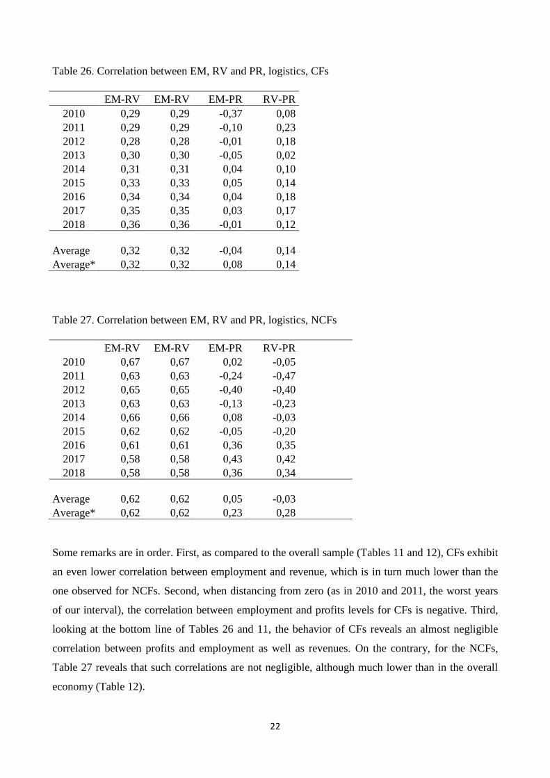
Table 26. Correlation between EM, RV and PR, logistics, CFs
EM-RV EM-RV EM-PR RV-PR
2010 0,29 0,29 -0,37 0,08
2011 0,29 0,29 -0,10 0,23
2012 0,28 0,28 -0,01 0,18
2013 0,30 0,30 -0,05 0,02
2014 0,31 0,31 0,04 0,10
2015 0,33 0,33 0,05 0,14
2016 0,34 0,34 0,04 0,18
2017 0,35 0,35 0,03 0,17
2018 0,36 0,36 -0,01 0,12
Average 0,32 0,32 -0,04 0,14
Average* 0,32 0,32 0,08 0,14
Table 27. Correlation between EM, RV and PR, logistics, NCFs
EM-RV EM-RV EM-PR RV-PR
2010 0,67 0,67 0,02 -0,05
2011 0,63 0,63 -0,24 -0,47
2012 0,65 0,65 -0,40 -0,40
2013 0,63 0,63 -0,13 -0,23
2014 0,66 0,66 0,08 -0,03
2015 0,62 0,62 -0,05 -0,20
2016 0,61 0,61 0,36 0,35
2017 0,58 0,58 0,43 0,42
2018 0,58 0,58 0,36 0,34
Average 0,62 0,62 0,05 -0,03
Average* 0,62 0,62 0,23 0,28
Some remarks are in order. First, as compared to the overall sample (Tables 11 and 12), CFs exhibit
an even lower correlation between employment and revenue, which is in turn much lower than the
one observed for NCFs. Second, when distancing from zero (as in 2010 and 2011, the worst years
of our interval), the correlation between employment and profits levels for CFs is negative. Third,
looking at the bottom line of Tables 26 and 11, the behavior of CFs reveals an almost negligible
correlation between profits and employment as well as revenues. On the contrary, for the NCFs,
Table 27 reveals that such correlations are not negligible, although much lower than in the overall
economy (Table 12).

23
Notwithstanding the aforementioned peculiarities, we can summarize our analysis of the regional
logistics industry as follows. Here, more than in the entire economy, CFs seem to care more about
employment than about profits. As compared to NCFs, the CFs attitude of protecting employees17 is
associated with a poorer performance in terms of labor productivity, as it is evident from the lower
level of both revenue per worker and aggregate profits.
5. Conclusions
In this paper we investigate the ER economy in order to shed light on the differences between the
performance of cooperative firms and the conventional ones. A related key question we aimed at
tackling deals with the objective function of cooperative firms as apparently revealed by their
decisions. We employ a unique data set covering the entire universe of firms registered in ER from
which we select appropriately the sample. Our statistically descriptive analysis, although simple,
allows us to underline that: CFs are larger, in terms of employees, than NCFs; a “size effect” seems
at work in driving differences between CFs and NCFs; CFs tend to act countercyclically, or at least
more resiliently than NCFs during downturns; CFs tend to stabilize employment by sacrificing
profits.
As for the last evidence, we argue that our analysis seems to support the model by Kahana and
Nitzan (1989) and the predecessors of their approach: their formulation of the objective function of
CFs finds in our paper an empirical validation. Hence, the assumption of maximizing employment
under a profit constraint (or, equivalently, maximizing profits under an employment constraint) not
only normally avoids perverse effects, but it fits quite squarely the empirical evidence offered in
this paper as well as in previous empirical research. In other words, Kahana and Nitzan (1989)’s
approach appears capable of overcoming both objections that we can address (as we did in Section
1) to the original Ward (1958)’s formulation of cooperatives’ goal (labor-managed firms’, in his
own world).
A subtle issue may arise when observing countercyclical behavior by CFs because this may
seemingly echo Ward’s perverse effect. However, it is easy to relate our empirical findings, on the
one hand, and some testable predictions stemming from the approach modeled by Kahana and
Nitzan (1989) as well as the setting considered by Ward (1958), on the other. Indeed, both Ward
(1958) and Kahana and Nitzan (1989) assume price-taking behaviour and ideal (in the sense of
17 All workers or mainly the member ones; this is an aspect that would require knowing at least the average
membership ratio which is unfortunately unavailable, also because, as we know, most CFs of the logistics do
not adhere to any cooperative association.
24
Sertel’s workers’ firms) LMFs, while our sample is extracted from real oligopolistic markets where
profit-maximizing firms cohabit with heterogeneous (as for the operating sector, the nature of their
membership and being cooperative firms or joint stock companies controlled by cooperative firms)
CFs in which the membership ratio is sizably lower than one. The basic difference between Ward’s
and Kahana and Nitzan’s models deals with the specification of the objective function. Hence,
notwithstanding they share some assumptions, the different formulation about what cooperatives are
supposed to maximize is crucial enough to yield very different properties of the resulting
comparative statics. Our empirical findings seem to support the view, captured by Kahana and
Nitzan (1989)’s behavioral assumption, that CFs do care about their own employment levels even if
it entails sacrificing profitability.
There is another implication of our results. It is by now well known that the main source of income
inequality is labour income inequality18. Hence, to shrink the former, actions to reduce the latter are
in order. By preserving employment, especially during slums, CFs participate in the process of
containing labour income inequality because unemployment, by zeroing market revenues of a
fraction of labor force, cannot but uplift income inequality. We may claim that CFs strategies
operate as an ex-ante redistributive mechanism, as opposed to ex-post public policies designed to
mitigate the consequences of falls in labour incomes19. Moreover, we know that the pay-ratio within
CFs employees (at least in cooperative firms, not necessarily in companies controlled by
cooperatives) is usually lower than in NCFs20. By limiting wage dispersion between white collars
and blue collars, CFs provides another contribution to limit, once again ex-ante, an exceedingly
high-income inequality among their employees and then, given their critical mass, also within the
employed in ER as a whole.
Last but not least, we believe that, while showing how different regional producers reacted to the
financial crisis and the subsequent recession, our empirical analysis may also establish a fairly
18 See, for instance, the interesting contribution by Milanovic (2019) and the large bibliography cited there.
19 This is particularly true in social CFs which function combining workers and users of a vast range of social
services and hire people with profiles in high risk of employment exclusion. Incidentally, excluding the
constructions sector, anecdotical evidence indicates that during recessions CFs have resorted to social
welfare nets in lower proportions than their NCFs counterparts. According to Kruse (2016, p. 1), a large
empirical evidence suggests that: “Employee ownership companies have more stability, higher survival rates,
and fewer layoffs in recessions, potentially leading to lower unemployment in the overall economy. … The
broader sharing of economic rewards may help reduce economic inequality.” Production cooperatives belong
to such a category of companies.
20 For instance, in its ethical code, Legacoop sets an upper bound of 8 between the values of the highest and
the lowest salary within the various layers of their organization.

25
useful benchmark to assess in due time the economic effects of the pandemic severely hitting also
the ER economy.
26
References
Burdin, C. and A. Dean (2009), “New evidence on wages and employment in worker cooperatives
compared with capitalist firms”, Journal of Comparative Economics, 37, 517-33.
Burdin, C. and A. Dean (2012), “Revisiting the objectives of worker cooperatives: an empirical
assessment”, Economic Systems, 36, 158-71.
Clemente, J., M. Diaz-Fonced, C. Maruello, and M. Sanso-Navarro (2012), “The wage gap between
cooperative and capitalist firms: evidence from Spain”, Annals of Public and Cooperative
Economics, 83, 337-56.
Costa, M. (2016), “Overlapping component and inequality decomposition: a simulation study for
the Gini index”, Metron, 74, 193-205.
Craig, B. and J. Pencavel (1992), “The behaviour of workers cooperatives: the plywood companies
of the Pacific Northwest”, American Economic Review, 82, 1083-105.
Craig, B. and J. Pencavel (1993), “The objectives of workers cooperatives”, Journal of
Comparative Economics, 17, 288-308.
Craig, B. and J. Pencavel (1995), “Participation and productivity: a comparison of workers
cooperatives and conventional firms in the plywood industry”, Brookings Papers on Economic
Activity, 26, 121-74.
Dagum, C. (1997), “A new decomposition of the Gini income inequality ratio”, Empirical
Economics, 22, 515-31.
Delbono, F. and G. De Fraja (1990), “Game theoretic models of mixed oligopoly”, Journal of
Economic Surveys, 4, 1-17.
Delbono, F. and L. Lambertini (2014), “Cartel size and collusive stability with non-capitalistic
players”, Economics Letters, 125, 156-9.
Delbono, F. and C. Reggiani (2013), “Cooperative firms and the crisis: evidence from some Italian
mixed oligopolies”, Annals of Public and Cooperative Economics, 84, 383-97.
Delbono, F. and G. Rossini (1992), “Competition policy vs horizontal merger with public,
entrepreneurial and labor-managed firms”, Journal of Comparative Economics, 16, 226-40.
Euricse (2020), “Exploring the co-operative economy”, Report 2020.
Fellner, W. (1947), “Prices and wages under bilateral monopoly”, Quarterly Journal of Economics,
61, 503-32.
Gal-or, E., M. Landsberger and A. Subotnik (1980), “Allocative and distributional effects of a
monopolistic cooperative firm in a capitalist economy”, Journal of Comparative Economics, 4, 158-
72.
Giorgi, G.M. (2011), “The Gini inequality index decomposition. An evolutionary study”, in
Deutsch, J. and J. Silber (eds.), The measurement of individual well-being and group inequalities,
185–218, London, Routledge.
27
International Cooperative Alliance (2017), “Co-operatives and employment”.
Kahana, N. and S. Nitzan (1989), “More on alternative objectives of labor-managed firms”, Journal
of Comparative Economics, 13, 527-38.
Kruse, D. (2016), “Does employee ownership improve performance?” IZA World of Labor, 311
Law, P. (1977) “The Ilyrian firm and Fellner’s union-management model”, Journal of Economic
Studies, 4, 29-37.
Milanovic, B. (2019), Capitalism. Alone. The future of the system that rules the world, Belknap
Press of Harvard University Press, Cambridge (Mass.).
Navarra, C. (2016), “Employment stabilization inside firms: an empirical investigation of worker
cooperatives”, Annals of Public and Cooperative Economics, 87, 563-85.
Perotin, V. (2006), “Entry, exit, and the business cycle: are cooperatives different?”, Journal of
Comparative Economics, 34, 295-316.
Perotin, V. (2012), “The performance of workers cooperatives”, in Battilani P. and H. Schroter
(eds.), The cooperative business movement, 1950 to the present, Cambridge University Press.
Regione Emilia-Romagna (2019), Rapporto Biennale sullo stato della cooperazione.
Sertel, M. (1982), Workers and incentives, North-Holland, Amsterdam.
Ward, B. (1958), “The firm in Ilyria: market syndicalism”, American Economic Review, 48, 566-89.
Zamagni, S. and V. Zamagni (2011), Cooperative Enterprise, Chelthenaum, Edward Elgar.
Zamagni, V. (2019), “Why we need cooperatives to make the business world more people-
centered”, presented at UNFTSSE International Conference, Geneve.
28
Appendix
Table 4A. Revenue (million euros, 2015 prices)
NCF % NCF CF % CF
2010 161.421 79,24 42.291 20,76
2011 175.933 79,03 46.694 20,97
2012 173.980 78,42 47.866 21,58
2013 181.584 76,27 56.481 23,73
2014 186.410 74,85 62.633 25,15
2015 190.693 75,85 60.731 24,15
2016 196.533 76,31 60.999 23,69
2017 214.238 77,25 63.080 22,75
2018 227.608 78,11 63.799 21,89
Table 5A. Number of employees
NCF % NCF CF % CF
2010 597.671 73,20 218.853 26,80
2011 595.291 72,37 227.222 27,63
2012 598.517 72,07 231.998 27,93
2013 595.706 70,84 245.200 29,16
2014 593.293 69,79 256.832 30,21
2015 610.156 70,06 260.778 29,94
2016 632.859 70,76 261.545 29,24
2017 668.166 71,53 265.973 28,47
2018 691.254 71,99 268.899 28,01
Table 7A. Employment, Gini decomposition
Gw Gb Go G
2010 0.504 0.222 0.039 0.765
2011 0.497 0.230 0.039 0.765
2012 0.498 0.233 0.038 0.769
2013 0.492 0.244 0.038 0.774
2014 0.488 0.254 0.037 0.780
2015 0.498 0.238 0.037 0.774
2016 0.494 0.248 0.036 0.778
2017 0.500 0.243 0.035 0.778
2018 0.505 0.240 0.034 0.779
29
Table 13A. Employees, small firms
NCF % NCF CF %CF
77.198 85,11 13.503 14,89
72.370 84,88 12.892 15,12
77.239 86,04 12.534 13,96
68.752 83,91 13.185 16,09
67.279 85,12 11.762 14,88
68.676 85,75 11.417 14,25
71.201 87,24 10.417 12,76
76.979 87,89 10.608 12,11
78.257 88,82 9.855 11,18
Table 15A. Employees, small firms, Gini decomposition
Gw Gb Go G
2010 0.393 0.095 0.026 0.514
2011 0.363 0.094 0.024 0.481
2012 0.400 0.086 0.027 0.513
2013 0.352 0.101 0.023 0.476
2014 0.354 0.091 0.023 0.468
2015 0.351 0.086 0.022 0.459
2016 0.358 0.074 0.021 0.453
2017 0.374 0.071 0.022 0.467
2018 0.376 0.065 0.021 0.461
Table 16A. Employees, large firms
NCF % NCF CF % CF
2010 520.473 71,71 205.350 28,29
2011 522.921 70,93 214.330 29,07
2012 521.278 70,37 219.464 29,63
2013 526.954 69,43 232.015 30,57
2014 526.014 68,22 245.070 31,78
2015 541.477 68,47 249.361 31,53
2016 561.658 69,10 251.128 30,90
2017 591.187 69,83 255.365 30,17
2018 612.997 70,29 259.044 29,71

30
Table 18A. Employees, large firms, Gini decomposition
Gw Gb Go G
2010 0.459 0.230 0.035 0.725
2011 0.455 0.238 0.034 0.727
2012 0.451 0.242 0.034 0.727
2013 0.451 0.250 0.034 0.735
2014 0.446 0.262 0.034 0.741
2015 0.446 0.262 0.034 0.741
2016 0.450 0.257 0.033 0.739
2017 0.456 0.252 0.032 0.740
2018 0.460 0.248 0.032 0.741
Table 19A. Number of CFs and NCFs, logistics
NCF % NCF CF % CF
2010 1.173 72,18 452 27,82
2011 1.199 73,56 431 26,44
2012 1.194 73,75 425 26,25
2013 1.192 73,95 420 26,05
2014 1.209 74,45 415 25,55
2015 1.266 75,58 409 24,42
2016 1.289 75,96 408 24,04
2017 1.345 77,34 394 22,66
2018 1.376 78,49 377 21,51
Table 20A. Revenue (million euros, 2015 prices), logistics
NCF % NCF CF % CF
2010 4.946 68,49 2.275 31,51
2011 5.403 69,40 2.382 30,60
2012 5.593 69,79 2.420 30,21
2013 5.684 70,47 2.381 29,53
2014 5.838 70,70 2.420 29,30
2015 6.147 70,51 2.571 29,49
2016 6.101 70,34 2.572 29,66
2017 6.509 70,32 2.747 29,68
2018 6.887 70,93 2.823 29,07

31
Table 21A. Number of employees, logistics
NCF % NCF CF % CF
2010 22.247 49,74 22.479 50,26
2011 21.407 49,57 21.780 50,43
2012 22.464 50,67 21.866 49,33
2013 22.029 49,92 22.102 50,08
2014 22.620 48,17 24.337 51,83
2015 23.903 50,06 23.841 49,94
2016 24.437 49,42 25.009 50,58
2017 26.279 51,44 24.807 48,56
2018 27.700 53,03 24.537 46,97
