what do latin american inflation targeters care about? a
TRANSCRIPT

gareth.jones Section name
© Department of Economics, University of Reading 2016
What Do Latin American Inflation Targeters Care About? A Comparative Bayesian Estimation of Central Bank Preferences
by Stephen McKnight, Alexander Mihailov
and Antonio Pompa Rangel
Department of Economics Economic Analysis Research Group (EARG)
Discussion Paper No. 129 Department of Economics University of Reading Whiteknights Reading RG6 6AA United Kingdom www.reading.ac.uk


What Do Latin American Inflation Targeters Care About? A
Comparative Bayesian Estimation of Central Bank Preferences∗
Stephen McKnight,† Alexander Mihailov‡ and Antonio Pompa Rangel§
November 2016
Abstract
This paper uses Bayesian estimation techniques to uncover the central bank preferences
of the big five Latin American inflation targeting countries: Brazil, Chile, Colombia, Mex-
ico, and Peru. The target weights of each central bank’s loss function are estimated using
a medium-scale small open economy New Keynesian model with incomplete international
asset markets and imperfect exchange-rate pass-through. Our results suggest that all central
banks in the region place a high priority on stabilizing inflation and interest rate smoothing.
While stabilizing the real exchange rate is a concern for all countries except Brazil, only
Mexico is found to assign considerable weight to reducing real exchange rate fluctuations.
Overall, Brazil, Colombia, and Peru show evidence of implementing a strict inflation tar-
geting policy, whereas Chile and Mexico follow a more flexible policy by placing a sizeable
weight to output gap stabilization. Finally, the posterior distributions for the central bank
preference parameters are found to be strikingly different under complete asset markets.
This highlights the sensitivity of Bayesian estimation, particularly when uncovering central
bank preferences, to alternative international asset market structures.
JEL codes: C51, E52, F41.
Keywords: Bayesian estimation, central bank preferences, inflation targeting, Latin Amer-ica, small open economies, incomplete asset markets, monetary policy.
∗We are grateful to Julio Carrillo, Jesús Fernández-Villaverde, Kólver Hernández, Timothy Kam, AlbertoOrtiz, Jessica Roldán, and Konstantinos Theodoridis for helpful comments and suggestions. Feedback from theaudiences at seminars at Banco de México and El Colegio de México, at the workshops on “How Should DSGEModels Be Estimated?” and on “Bayesian Computation” at the University of Reading, and at the LACEA-LAMES 2016 in Medellín is also acknowledged. We are indebted to Timothy Kam and Alejandro Justiniano forkindly providing their Matlab codes. The usual disclaimer applies. The views expressed herein are those of theauthors and do not necessarily reflect those of Banco de México.†Centro de Estudios Económicos, El Colegio de México, Camino al Ajusco 20, Col. Pedregal de Santa Teresa,
Mexico City, 10740, Mexico. E-mail: [email protected].‡Department of Economics, University of Reading, Whiteknights, PO Box 218, Reading, RG6 6AA, United
Kingdom. E-mail: [email protected].§Dirección General de Investigación Económica, Banco de México, Calle 5 de Mayo 18, Col. Centro, Mexico
City, 06069, Mexico. E-mail: [email protected].

Contents
1 Introduction 1
2 The Model 32.1 Households . . . . . . . . . . . . . . . . . . . . . . . . . . . . . . . . . . . . . . . 3
2.2 Domestic Good Producers . . . . . . . . . . . . . . . . . . . . . . . . . . . . . . . 5
2.3 Retail Firms . . . . . . . . . . . . . . . . . . . . . . . . . . . . . . . . . . . . . . . 6
2.4 Market Clearing . . . . . . . . . . . . . . . . . . . . . . . . . . . . . . . . . . . . 7
2.5 The Log-Linearized Model . . . . . . . . . . . . . . . . . . . . . . . . . . . . . . . 7
2.6 Central Bank Preferences . . . . . . . . . . . . . . . . . . . . . . . . . . . . . . . 9
3 Estimation 93.1 Data . . . . . . . . . . . . . . . . . . . . . . . . . . . . . . . . . . . . . . . . . . . 9
3.2 Methodology and Prior Selection . . . . . . . . . . . . . . . . . . . . . . . . . . . 10
4 Results 114.1 Model Comparison, Posterior Shapes and Convergence Diagnostics . . . . . . . . 11
4.2 Estimated Structural Parameters Influencing the Endogenous Propagation . . . . 13
4.3 Estimated Persistence and Volatility of the Latent Exogenous Shock Processes . 14
4.4 Complete versus Incomplete International Financial Markets . . . . . . . . . . . 14
5 Conclusions 15
List of Figures
1 Brazil —Posterior Distributions of the Structural Parameters (µq > 0) . . . . . . 22
2 Brazil —Posterior Distributions of the Structural Parameters (µq = 0) . . . . . . 23
3 Chile —Posterior Distributions of the Structural Parameters (µq > 0) . . . . . . . 24
4 Colombia —Posterior Distributions of the Structural Parameters (µq > 0) . . . . 25
5 Colombia —Posterior Distributions of the Structural Parameters (µq = 0) . . . . 26
6 Mexico —Posterior Distributions of the Structural Parameters (µq > 0) . . . . . . 27
7 Peru —Posterior Distributions of the Structural Parameters (µq > 0) . . . . . . . 28
List of Tables
1 The 6 Latin American Inflation Targeters: Some Basic Facts . . . . . . . . . . . 29
2 Prior Distributions . . . . . . . . . . . . . . . . . . . . . . . . . . . . . . . . . . . 30
3 Model Comparison and Estimated Policy Weights . . . . . . . . . . . . . . . . . . 31
4 Brazil: Posterior Parameters and Convergence Diagnostics (µq > 0) . . . . . . . . 32
5 Brazil: Posterior Parameters and Convergence Diagnostics (µq = 0) . . . . . . . . 33
6 Chile: Posterior Parameters and Convergence Diagnostics (µq > 0) . . . . . . . . 34

7 Colombia: Posterior Parameters and Convergence Diagnostics (µq > 0) . . . . . . 35
8 Colombia: Posterior Parameters and Convergence Diagnostics (µq = 0) . . . . . . 36
9 Mexico: Posterior Parameters and Convergence Diagnostics (µq > 0) . . . . . . . 37
10 Peru: Posterior Parameters and Convergence Diagnostics (µq > 0) . . . . . . . . 38
11 Model Comparison under Complete Asset Markets . . . . . . . . . . . . . . . . . 39


McKnight, Mihailov and Pompa Rangel (November 2016) 1
1 Introduction
For many central banks in both developed and developing countries, inflation targeting (IT)
has become the operational monetary framework of choice to achieve price stability.1 According
to the International Monetary Fund (IMF) (see, e.g., Jahan, 2012), since the adoption of IT
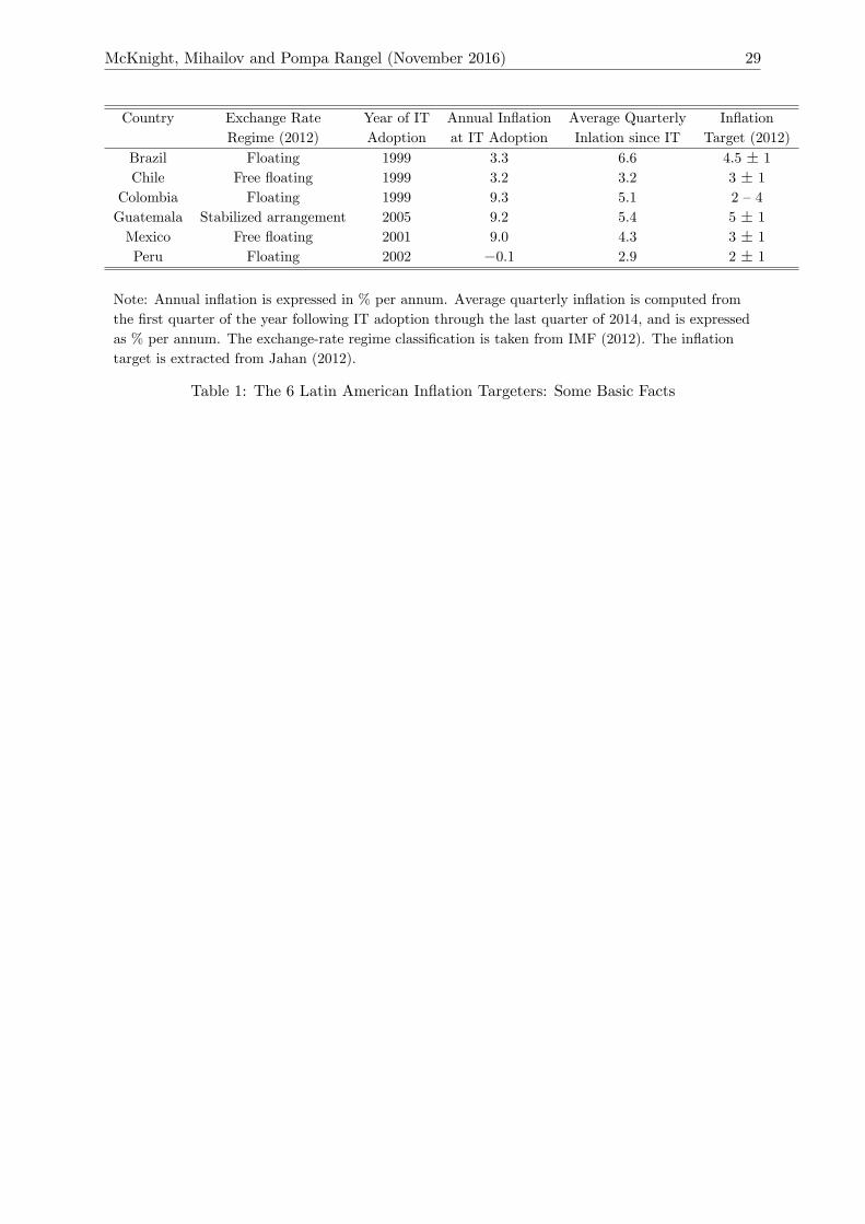
by New Zealand in December 1989, there are now 28 IT central banks worldwide, of which 6
currently originate from Latin America: Brazil, Chile and Colombia all adopted IT in 1999,
shortly followed by Mexico (2001), Peru (2002), and Guatemala (2005) (see Table 1).2 While
there is some empirical evidence to suggest that IT has been successful in reducing inflation in
developing countries (see, e.g., Batini and Laxton, 2007; Goncalves and Salles, 2008; Lin and
Ye, 2009; Lee, 2011),3 little is known about the policy preferences of central banks operating in
these countries.4 As discussed by Castelnuovo and Surico (2004) and Ilbas (2010, 2012), such
information can help in evaluating the performance of central banks, as well as improving our
understanding of monetary policy actions and its effects on the formation of expectations by
private agents.
The aim of this paper is to use Bayesian estimation techniques to uncover and compare
the central bank preferences of the big five Latin American inflation targeting (LAIT) coun-
tries.5 Since the IT framework can be considered as “constrained discretion” (Bernanke and
Mishkin, 1997), we assume that in each country monetary policy is conducted under discretion.
Each central bank is assumed to optimally set the nominal interest rate by minimizing an in-
tertemporal quadratic loss function that includes four specific policy objectives: price stability
via control of inflation, stabilizing the output gap, reducing real exchange rate variability, and
nominal interest rate smoothing. The weight attributed to each policy objective will depend on
the institutional preferences of each central bank, which we can make inferences about using
estimates of the respective Bayesian posterior distributions.
The structural model used to represent the LAIT economies is a dynamic medium-scale
small open economy New Keynesian model. Following the modeling frameworks of Monacelli
(2005), Kam et al. (2009) and Justiniano and Preston (2010), we allow for imperfect exchange-
rate pass-through (ERPT) such that the law of one price fails to hold. As in Adolfson et
al. (2007) and Justiniano and Preston (2010), international asset markets are assumed to
be incomplete such that consumption risk sharing is not perfect. Both these features have
been identified as empirically relevant, the more so for developing countries as in our sample.
Using the popular Random-Walk Metropolis-Hastings Markov Chain Monte Carlo algorithm,
we present posterior estimates and convergence diagnostics for both the structural parameters
and the persistence and standard deviations of the shocks we consider as most important in
1See, for example, Mishkin and Schmidt-Hebbel (2001), Carare and Stone (2006), Roger (2010), Hammond(2011), Jahan (2012).
2As Table 1 reveals, there is significant heterogeneity across these 6 Latin American countries in terms of theinflation target set and their performance in steering actual inflation towards the target.
3Lee (2011) finds that IT has been particularly successful in reducing inflation in Colombia, while no significantreductions were found for Chile. In contrast to much of the earlier literature, Brito and Bystedt (2010) find noevidence that IT improves economic performance in developing countries, as measured by the behavior of inflationand output growth.
4There is also some evidence to suggest that IT has reduced the dispersion of long-run inflation expectationsin developing countries. See Capistrán and Ramos-Francia (2010) for further details.
5We exclude Guatemala from the analysis due to the lack of reliable data.

What Do Latin American Inflation Targeters Care About? 2
emerging market economies (such as, among others, shocks to preferences, the risk premium,
the terms of trade, and technology).
Our main findings are as follows. First, all five central banks are strongly concerned about
stabilizing inflation and smoothing the nominal interest rate. In particular, relative to the weight
of inflation stabilization, we find that Brazil and Peru place very high weights on interest rate
smoothing. Second, there is significant heterogeneity amongst the five central banks concerning
the priorities of output gap stabilization and real exchange rate stabilization. Brazil, Colombia,
and Peru show little concern for the stabilization of the output gap, whereas Chile and Mexico
assign sizeable weights. While Brazil and Colombia are not concerned about real exchange rate
volatility, for the remaining three countries only Mexico is found to assign a suffi ciently high
weight to minimizing real exchange rate fluctuations. Overall, Brazil, Colombia and Peru show
evidence of implementing a strict inflation targeting policy, whereas Chile and Mexico appear
much more flexible in terms of their inflation targeting preferences.
In terms of the estimated key structural parameters influencing the endogenous propagation
mechanism of the model, we find that these are statistically reliable, economically plausible,
and broadly comparable to analogous estimates for other countries available in the literature
using non-Bayesian econometric methods. For example, the estimated elasticity of substitution
between home and foreign goods is within the typical range reported in Corsetti et al. (2008).
Furthermore, we uncover some interesting differences across countries. For example, the degree
of price stickiness in Brazil and Mexico is estimated to be over 3.5 times higher than in Peru.
In terms of the sources of exogenous fluctuations affecting the five LAIT economies, our
results indicate a high volatility (measured by the posterior mean standard deviation) for the
preference shock, the risk premium shock and the terms of trade shock. The most persistent
shock appears to be the risk premium shock, yet it does not dominate the persistence of some
among the other shocks in each individual country. Overall, the least persistent shock in all five
LAIT economies is the preference shock.
There are few papers that have used Bayesian techniques to estimate central bank preferences
in an open-economy setting.6 Kam et al. (2009) estimate the central bank preferences for
three developed IT countries, Australia, Canada, and New Zealand under optimal discretionary
monetary policy. They find that the central banks of these countries all have very similar
preferences: the highest priority is inflation stabilization, followed by interest rate smoothing,
with no concern for stabilizing the output gap (with the exception of Australia) and the real
exchange rate. Palma and Portugual (2014) estimate the model of Kam et al. (2009) using
Brazilian data. They find that the major concern was inflation stabilization, followed by interest
rate smoothing, real exchange rate stabilization and output gap stabilization.
While the estimation approach adopted in this paper is similar to Kam et al. (2009), one
important difference relates to the asset market assumption used in the structural model. Kam
et al. (2009) assume complete international asset markets which implies perfect risk sharing in
consumption and a strong positive correlation between the real exchange rate and the marginal
utilities of consumption across countries. However, there is clear empirical evidence for both de-
6 In a closed-economy setting, Ilbas (2010, 2012) estimates the preferences of the European Central Bank andthe US Federal Reserve under commitment using the structural models of Smets and Wouters (2003, 2007).
McKnight, Mihailov and Pompa Rangel (November 2016) 3
veloped and developing economies of low consumption risk sharing across countries.7 Moreover,
Rabanal and Tuesta (2010) show that the extent of international financial market integration af-
fects both the Bayesian estimates of the parameters and the transmission mechanism of shocks.
We therefore depart from Kam et al. (2009) and follow the modeling approach of Adolfson et
al. (2007) and Justiniano and Preston (2010) in assuming incomplete international financial
markets in addition to imperfect ERPT.8 Furthermore, we test the sensitivity of our results to
the alternative assumption of complete asset markets and show that a number of our key policy
conclusions obtained under incomplete asset markets are now reversed. This is consistent with
the Bayesian analysis of Rabanal and Tuesta (2010) who also find that the degree of model
misspecification depends on the asset market structure.9 Overall, our sensitivity analysis em-
phasizes the dangers of using the complete asset markets assumption in Bayesian estimation,
particularly when uncovering central bank prevalences.
The paper is organized as follows. Section 2 outlines the theoretical model. Section 3
describes the data and explains the estimation strategy. Section 4 reports our main results.
Finally, section 5 concludes.
2 The Model
This section outlines the model economy, which is based on the SOE frameworks of Monacelli
(2005), Kam et al. (2009), and Justiniano and Preston (2010). The domestic economy is popu-
lated by infinitely-lived households of measure one, a continuum of domestic good producers, a
continuum of retail firms who import foreign goods at competitive world prices, and a central
bank. Both domestic and retail firms are assumed to operate under monopolistic competition
and set prices in a staggered fashion according to Calvo (1983). Market power in the retail sec-
tor for imported goods results in incomplete ERPT and thus the law of one price fails to hold.
International financial markets are assumed to be incomplete. Following Kam et al. (2009), the
inflation-targeting central bank is assumed to minimize a quadratic loss function under discre-
tion. In what follows, asterisks conventionally denote foreign variables, and subscripts H (F )
denote variables of Home (Foreign) origin.
2.1 Households
Households consume a composite of domestic CH and imported CF goods:
Ct =
[(1− α)
1nC
η−1η
H,t + α1nC
η−1η
F,t
], (1)
CH,t =
[∫ 1
0CH,t(i)
ε−1ε di
] εε−1
; CF,t =
[∫ 1
0CF,t(j)
ε−1ε dj
] εε−1
. (2)
7See, e.g., Chari et al. (2002), Heathcote and Perri (2002), Corsetti et al. (2008), Rabanal and Tuesta (2010),Raffo (2010).
8Justiniano and Preston (2010) estimate the coeffi cients of a Taylor-type monetary policy rule for the samethree advanced IT economies as in Kam et al. (2009).
9Using Bayesian estimation of a medium-scale two-country model for the US and the Euro Area, they findthat incomplete asset markets fits the data better than complete asset markets, including matching the dynamicsof the real exchange rate.

What Do Latin American Inflation Targeters Care About? 4
The parameter η > 0 measures the elasticity of substitution between home and foreign goods,
α ∈ (0, 1) is the share of foreign goods in the domestic consumption bundle, and ε > 1 measures
the elasticity of substitution between the varieties of goods produced within H or F , where
i, j ∈ [0, 1]. The optimal allocation of expenditures between domestic and imported goods
yields the following aggregate demand conditions:
CH,t = (1− α)
(PH,tPt
)−ηCt, CF,t = α
(PF,tPt
)−ηCt, (3)
where the consumer price index Pt is given by:
Pt =[(1− α)P 1−ηH,t + αP 1−ηF,t
] 11−η
. (4)
The (home) real exchange rate qt is defined by
qt = etP ∗tPt, (5)
where et denotes the (home) nominal exchange rate. The relative price of foreign goods in terms
of home goods, or the (home) terms of trade, St, is expressed as
St =PF,tPH,t
. (6)
The representative household chooses consumption Ct and labor Nt to maximize expected
discounted utility:
maxE0∞∑t=0
βtεg,tU
((Ct −Ht)
1−σ
1− σ − N1+ϕt
1 + ϕ
),
where the discount factor is β ∈ (0, 1), σ, ϕ > 0 are the inverse elasticities of intertemporal
substitution and labor supply, respectively, Ht ≡ hCt−1 is an external habit variable with
h ∈ (0, 1), and εg,t is a preference shock.
The household during period t supplies labor to domestic firms receiving income from wages
Wt and profits from the ownership of domestic and retail firms Πt. As in Adolfson et al. (2007)
and Justiniano and Preston (2010) — but differently from Monacelli (2005) and Kam et al.
(2009) —the international asset market structure is assumed to be incomplete. Let Bt−1 and
B∗t−1 denote the holdings of home and foreign risk-free bonds that mature in period t with
corresponding interest rates rt and r∗t . Following Justiniano and Preston (2010), we assume
that there is a debt-elastic interest rate premium ωt−1(Dt−1, εq,t−1) given by:
ωt−1 = exp[−χ(Dt−1 + εq,t−1)], Dt−1 ≡et−1B∗t−1YssPt−1
, (7)
where εq,t−1 is a risk premium shock and Dt−1 is defined as the ratio of the real quantity of
foreign bond holdings (expressed in terms of domestic currency) to steady state output Yss.
If the household is a borrower (Dt > 0), it must pay a premium over the interest rate. This

McKnight, Mihailov and Pompa Rangel (November 2016) 5
debt-elastic interest rate premium is suffi cient to ensure that bond holdings are stationary.10
Consequently, the period budget constraint of the domestic household can be expressed as:
PtCt +Bt + etB∗t = Bt−1(1 + rt−1) + etB
∗t−1(1 + r∗t−1)ωt−1(Dt−1) +WtNt + Πt. (8)
The first-order conditions from the households maximization problem yield:
(Ct −Ht)σNϕ
t =Wt
Pt, (9)
β(1 + rt)Et
{(Ct+1 −Ht+1
Ct −Ht
)−σ ( PtPt+1
)(εg,t+1εg,t
)}= 1, (10)
Et{εg,t+1(Ct+1 −Ht+1)
−σ
Pt+1
[(1 + rt)− (1 + r∗t )
(et+1et
)ωt(Dt, εq,t)
]}= 0. (11)
Equation (9) is the intratemporal labor supply condition, (10) is the intertemporal consumption
Euler equation, and (11) is the interest rate parity condition.
2.2 Domestic Good Producers
The domestic goods market is comprised of a continuum of monopolistically competitive firms
i ∈ [0, 1] that produce differentiated goods. Domestic firms hire labor N to produce output
using a linear production technology
YH,t(i) = εa,tNt(i), (12)
where εa,t is an exogenous domestic technology shock, and given competitive prices of labor,
cost minimization yields
MCt =Wt
εa,tPH,t, (13)
where MCt denotes real marginal cost.
Domestic firms set prices according to Calvo (1983), where in each period there is a constant
probability 1 − θH that a firm will be randomly selected to adjust its price, while a fraction
0 < θH < 1 adjusts their prices according to the following indexation rule
PH,t(i) = PH,t−1(i)
(PH,t−1PH,t−2
)δH, (14)
where δH ∈ [0, 1] measures the degree of inflation indexation. For simplicity, we assume that
the export price of the domestic good is determined by the law of one price: P ∗Ht = (1/St)PH,t.
A domestic firm i, faced with changing its price at time t, has to choose PH,t(i) to maximize its
expected discounted value of profits:
maxPH,t(i)
Et∞∑s=0
Qt,t+sθsH
[PH,t(i)
(PH,t+s−1PH,t−1
)δH− PH,t+sMCt+s exp(εH,t+s)
]YH,t+s(i),
10For an in-depth discussion of the stationarity problem of small open-economy models with incomplete assetmarkets, see Schmitt-Grohé and Uribe (2003).

What Do Latin American Inflation Targeters Care About? 6
where
YH,t+s(i) =
(PH,t(i)
PH,t+s
(PH,t+s−1PH,t−1
)δH)−ε(CH,t+s + C∗H,t+s), (15)
and εH,t is a cost-push shock. The first-order condition is:
Et∞∑s=0
Qt,t+sθsHYH,t+s(i)
[PH,t
(PH,t+s−1PH,t−1
)δH−(
ε
ε− 1
)PH,t+sMCt+s exp(εH,t+s)
]= 0.
(16)
The aggregate price level evolves according to:
PH,t =
(1− θH)(PH,t)1−ε + θH
(PH,t−1
(PH,t−1PH,t−2
)δH)1−ε 11−ε
. (17)
2.3 Retail Firms
The retail market is comprised of a continuum of monopolistically competitive firms j ∈ [0, 1]
that import differentiated goods from abroad. Similar to domestic firms, retail firms also set
prices according to Calvo (1983) where in each period there is a constant probability 1 − θFthat a retail firm will be randomly selected to adjust its price.11 Faced with changing its price
at time t, a retail firm j importing a good at cost etP ∗F,t(j) chooses PF,t(j) to maximize its
expected discounted value of profits:
maxPF,t(j)
Et∞∑s=0
Qt,t+sθsF
[PF,t(j)
(PF,t+s−1PF,t−1
)δF− et+sP ∗F,t+s(j) exp(εF,t+s)
]YF,t+s(j), (18)
where
YF,t+s(j) =
[PF,t(j)
PF,t+s
(PF,t+s−1PF,t−1
)δF ]−εCF,t+s, (19)
and εF,t is a cost-push shock to import retailers. The first-order condition is given by:
Et∞∑s=0
Qt,t+sθsFYF,t+s(j)
[PF,t
(PF,t+s−1PF,t−1
)δF−(
ε
ε− 1
)et+sP
∗F,t+s(j) exp(εF,t+s)
]= 0, (20)
and the aggregate price index for imports:
PF,t =
(1− θF )(PF,t)1−ε + θF
(PF,t−1
(PF,t−1PF,t−2
)δF)1−ε 11−ε
. (21)
11The parameter θF governs the degree of ERPT.
McKnight, Mihailov and Pompa Rangel (November 2016) 7
2.4 Market Clearing
Goods market clearing for domestic firms requires:
YH,t(i) = CH,t(i) + C∗H,t(i) =
(PH,t(i)
PH,t
)−ε [CH,t + C∗H,t
],
⇒ Yt ≡∫ 1
0YH,t(i)di = CH,t + C∗H,t,
(22)
where
C∗H,t = α
(P ∗H,tP ∗t
)−ηC∗t and Y ∗t = C∗t .
Market clearing for domestic bonds requires:
Bt = 0. (23)
2.5 The Log-Linearized Model
The model is log-linearized around a deterministic zero-inflation steady state where bond hold-
ings are zero and the terms of trade are equal to Sss = 1. Let lowercase letters denote the
log-deviations of the respective variables from their steady-state values: i.e., xt = ln(Xt/Xss).
Log-linearizing the consumption Euler equation of the domestic household (10) yields:
ct − hct−1 = Et(ct+1 − hct)−1− hσ
(rt − Etπt+1)−1− hσ
(Etεg,t+1 − εg,t). (24)
Log-linearizing (16) and (17) gives the aggregate supply condition for domestic goods:
πH,t − δHπH,t−1 = βEt(πH,t+1 − δHπH,t) +(1− βθH)(1− θH)
θH(mct + εH,t), (25)
where πH,t = pH,t − pH,t−1 and
mct = ϕyt − (1 + ϕ)εa,t + αst +σ
1− h(ct − hct−1),
which is obtained after combining (9), the aggregate version of (12), (13) and noting that the
log-linearized version of the CPI index (4) implies pt − pH,t = αst after using (6).
Log-linearizing (20) and (21) gives the aggregate supply condition for retail goods:
πF,t − δFπF,t−1 = βEt(πF,t+1 − δFπF,t) +(1− βθF )(1− θF )
θF(ψF,t + εF,t), (26)
where πF,t = pF,t − pF,t−1 and the law of one price gap ψF,t is defined as:
ψF,t ≡ et + p∗t − pF,t.

What Do Latin American Inflation Targeters Care About? 8
Log linearizing equations (4)—(6) and using the above definition of ψF,t yields the following
relationship for the real exchange rate and the terms of trade:
qt = et + p∗t − pt = ψF,t + (1− α)st. (27)
First-differencing the log-linearized version of equation (6) yields:
st − st−1 = πF,t − πH,t + εs,t, (28)
where εs,t is an exogenous terms of trade shock, and first-differencing the log-linearized version
of the CPI index (4) gives:
πt = (1− α)πH,t + απF,t, (29)
where πt = pt − pt−1.The real interest rate parity condition is obtained by first-differencing (27) and combining
with the log-linearized version of (11):
(rt − Etπt+1)− (r∗t − Etπ∗t+1) = Et(qt+1 − qt)− χ(dt + εq,t). (30)
The disturbance term εq,t captures time-varying deviations from real interest rate parity. Log-
linearizing the budget constraint (8) implies:12
ct + dt =dt−1β− α(st + ψF,t) + yt, (31)
where dt = log(Dt) ≡ log(etB∗t /YssPt) is domestic-currency real foreign bond holdings (relative
to steady state output). Finally, the goods market clearing condition (22) implies
yt = (1− α)ct + αηqt + αηst + αy∗t . (32)
We assume that the stochastic processes for preferences, technology, the terms of trade, and
risk-premium follow an independent AR(1) process:
εx,t = ρxεx,t−1 + vx,t, where ρx ∈ (0, 1), vx ∼ iid(0, σ2x) (33)
for x = g, a, s, q, and the cost-push shocks in the domestic and retail sectors follow an i.i.d.
process: εH ∼ i.i.d.(0, σH) and εF ∼ i.i.d. (0, σF ). Following Kam et al. (2009), we further
assume that the foreign country variables {π∗, y∗, r∗} follow uncorrelated AR(1) processes: π∗ty∗tr∗t
=
a1 0 0
0 b2 0
0 0 c3
π∗t−1
y∗t−1r∗t−1
+
σπ∗ 0 0
0 σy∗ 0
0 0 σr∗
vπ∗,t
vy∗,t
vr∗,t
(34)
where vπ∗,t, vy∗,t, vr∗,t ∼ N(0, I3).
12Similar to Justiniano and Preston (2010), in equilibrium household nominal income WtNt + Πt = PH,tYt +(PF,t − etP
∗t )CF,t.

McKnight, Mihailov and Pompa Rangel (November 2016) 9
Given the specification for monetary policy, the processes for {εa,t, εg,t, εq,t, εs,t} and
{π∗t , y∗t , r
∗t } described by (33) and (34), and the cost-push shocks {εH,t, εF,t}, the system of equa-
tions (24)—(32) determines the following ten endogenous variables {ct, yt, dt, qt, st, ψF,t, rt, πt,πH,t, πF,t}.
2.6 Central Bank Preferences
As is standard in the literature, we assume that the central bank minimizes a one-period ad-hoc
quadratic loss function where monetary policy targets inflation, the output gap, and interest
rate smoothing.13 In addition, following Kam et al. (2009) the central bank can also target the
real exchange rate. Consequently, the loss function is given by:
L(πt, yt, qt, rt − rt−1) =1
2
[π2t + µyy
2t + µqq
2t + µr(rt − rt−1)2
]. (35)
The weight assigned to the annual inflation rate πt ≡∑3
i=0 πt−i/4 is normalized to one and the
weights µy, µq, µr ∈ [0,+∞) represent the relative importance assigned to output gap stabiliza-
tion, RER stabilization and interest rate smoothing. The loss function specification given by
(35) is consistent with flexible inflation targeting as described by Svensson (1999). Interest rate
smoothing is included to capture monetary policy inertia.14 As discussed by Svensson (2000),
the RER plays a prominent role in the monetary policy transmission mechanism in SOEs.
We further assume that the central bank minimizes (35) subject to the structural equations
(24)—(32) under discretion.15 We employ the algorithm of Dennis (2007) to compute solutions
to a linear-quadratic Markov perfect equilibrium (LQ-MPE) problem.16 Following Kam et al.
(2009), we add a noise term εr,t ∼ N(0, σ2r) to the resulting optimal interest rate rule rt(εt, zt−1)
to capture imperfections in the setting of interest rates (i.e., an exogenous monetary policy
shock).
3 Estimation
3.1 Data
To estimate the model we use quarterly data for each of the five LAIT countries. The Foreign
economy is proxied by the United States (US). All data were downloaded from the IMF’s Inter-
national Financial Statistics, the OECD’s National Accounts, and statistical tables published by
the central bank of each country. Since the LAIT countries switched to IT at different periods
during the late 1990s and early 2000s (see Table 1), the sample period differs for each country.
To remove any country-specific noise in the data, the first few years of data after the adoption
13An alternative approach would be to derive an approximate welfare-based loss function using the preferencesof the household. While this approach is theoretically appealing (see, e.g., Woodford, 2003; Galí, 2015), it doesnot carry over easily to open economies (see, e.g., Benigno and Benigno, 2003; Monacelli, 2005). In particular,an accurate quadratic approximation of household welfare can be obtained in open economy models only underspecial assumptions on household preferences and on the value of the trade elasticity parameter η.14See Ilbas (2012) and McKnight and Mihailov (2015) for further discussion on the reasons behind its inclusion.15When solving (35) under discretion, the central bank treats the problem as one of sequential optimization,
whereas under commitment, the central bank credibly commits to a policy plan.16For further details, see Dennis (2007) and Kam et al. (2009).
What Do Latin American Inflation Targeters Care About? 10
of IT were also omitted from the sample. Specifically, the sample period for each country used
in the estimations is as follows: 2004:1 —2014:4 for Brazil, 2002:1 —2014:4 for Chile, 2003:1 —
2014:4 for Colombia, 2002:1 —2014:4 for Mexico, and 2005:1 —2014:4 for Peru.
As the model features 10 exogenous shock processes {εa,t, εg,t, εq,t, εr,t, εs,t, εH,t, εF,t,
vπ∗,t, vr∗,t, vy∗,t}, 10 observable time series are needed to avoid stochastic singularity. Our
data set contains the following 10 observable variables: imported goods inflation denominated
in domestic currency (πF,t), the terms of trade (measured as the price of imports to exports)
(st), the real exchange rate (computed using the nominal exchange rate defined as national
currency per 1 USD) (qt), domestic real GDP (yt), domestic CPI inflation (πt), the nominal
interest rate (rt), US CPI inflation (π∗t ), US real output (y∗t ), and the US federal funds rate
(r∗t ). Consistent with the definition in (7), the foreign bond holdings ratio (dt) is proxied by
the real value of international reserves of each country converted into national currency by the
nominal exchange rate and divided by the Hodrick-Prescott trend in output. All variables are
expressed in logs and detrended using the Hodrick—Prescott filter, except inflation rates and
interest rates, which are expressed in quarterly percentage change. Since monetary policy in
our framework is driven using an output gap methodology, for yt we use the Hodrick—Prescott
filter to construct an output gap of deviations from the trend. As is customary in the estimation
of DSGE models analysis, all variables, including those in percentage terms, are demeaned to
approximate theoretical deviations from the steady state.
In order to assess whether a positive or zero weight for the real exchange rate is more probable
for the policy objectives of each central bank, we follow Kam et al. (2009) in estimating two
versions of the model, µq > 0 versus µq = 0 in (35), to see which is more probable (given the
same observables and shocks) via the comparison of Bayesian posterior odds.
3.2 Methodology and Prior Selection
The model M is estimated using Bayesian methods.17 We update the a priori beliefs about
the parameter vector θ, represented by the prior density p(θ|M) in view of the information
contained in the observed sample Y .18 According to Bayes Theorem (see, e.g., Herbst and
Schorfheide, 2016),
p(θ|Y,M) =p(Y |θ,M)p(θ|M)∫p(Y |θ,M)p(θ|M)dθ
, (36)
this updating generates a posterior distribution (or likelihood function) p(θ|Y,M). The denom-
inator in (36) is commonly known as the marginal likelihood of the data (or marginal data den-
sity) associated withM . As discussed by Herbst and Schorfheide (2016), among others, Bayesian
inference amounts to characterizing the properties of the posterior distribution p(θ|Y,M). Usu-
ally, posterior samplers are employed that generate sequences of draws θj , j = 1, ..., J from
p(θ|Y,M). As is common in the literature, we apply the Random-Walk Metropolis-Hastings
(RWMH) Markov Chain Monte Carlo (MCMC) algorithm to obtain draws from the posterior
17Bayesian methods are described in detail in Gelman et al. (2004) and Koop (2006), among others. Theirapplication to DSGE models has been expanding rapidly and includes key references such as Smets and Wouters(2003, 2007), An and Schorfheide (2007), Fernández-Villaverde et al. (2010), DeJong and Dave (2011), Del Negroand Schorfheide (2011), Miao (2014), Herbst and Schorfheide (2016), Fernández-Villaverde et al. (in press).18The parameter vector θ describes the preferences, technology, central bank policy weights, and exogenous
shock processes of the model M .
McKnight, Mihailov and Pompa Rangel (November 2016) 11
distribution.19 For each country, 2000000 RWMH-MCMC draws and 2500 Kalman filter iter-
ations were obtained, where the first half of the draws was discarded (or burnt-in) in order to
remove initial condition effects.
As the posterior density (36) is derived by combining the prior density p(θ|M) with the
likelihood function p(Y |θ,M), the selection of priors for each parameter plays a fundamental
role in Bayesian estimation. The priors used in our estimates are summarized in Table 2. As
is customary, we conform to the established conventions in selecting the prior densities: we use
the beta distribution for parameters in the interval [0, 1], the inverse gamma distribution for
the standard deviations of the stochastic innovations [0,∞), and the gamma distribution for
the rest.
Due to limited information in the data set, some structural parameters cannot be estimated
with suffi cient precision, and were therefore calibrated prior to estimation. For each country, we
calibrate the import share in domestic consumption, α, to values corresponding to the sample
average share of imports of goods and services in consumption: we set α to 0.20 for Brazil;
0.51 for Chile; 0.29 for Colombia; 0.44 for Mexico; and 0.35 for Peru.20 As is common in the
literature, for all countries the discount factor (β) is fixed at 0.99 and the debt-elastic interest
rate parameter (χ) is fixed at 0.05 consistent with the estimates of Selaive and Tuesta (2003 a,
b).21
In order not to add any prior information into the estimation stage, we follow Kam et
al. (2009) and assume that the prior distributions for the central bank preference parameters
µy, µq and µr are exactly the same. Consequently, any resulting differences in the posterior
distributions of these (as well as the other) parameters will be due to the data itself.
4 Results
For each of the five LAIT countries, Table 3 compares the characteristics of the Bayesian
RWMH-MCMC estimation for the two model versions, µq > 0 and µq = 0. This table also
presents a summary of the posterior mean and standard deviation estimates for the central
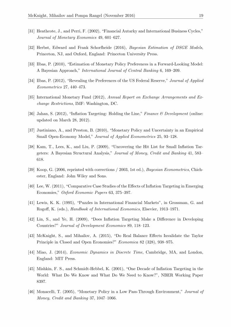
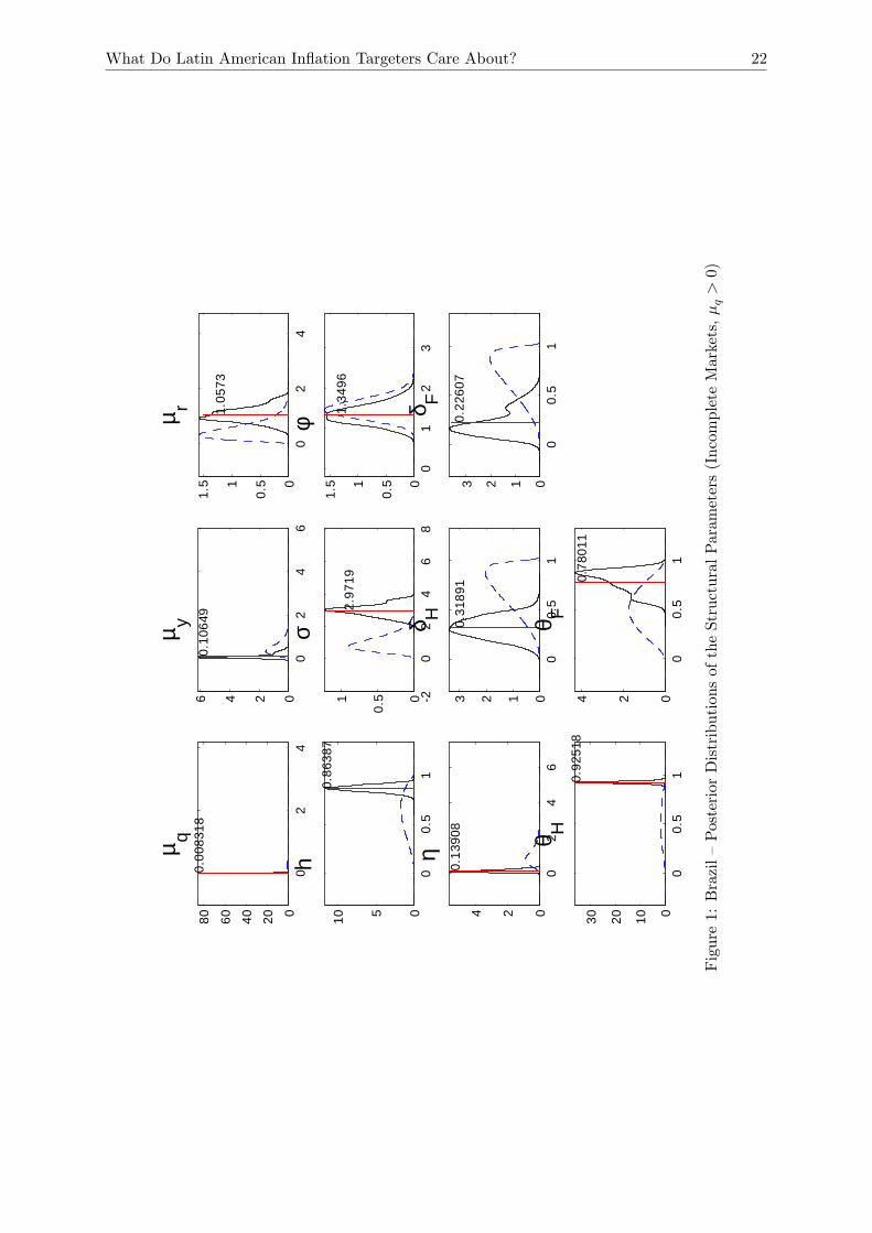
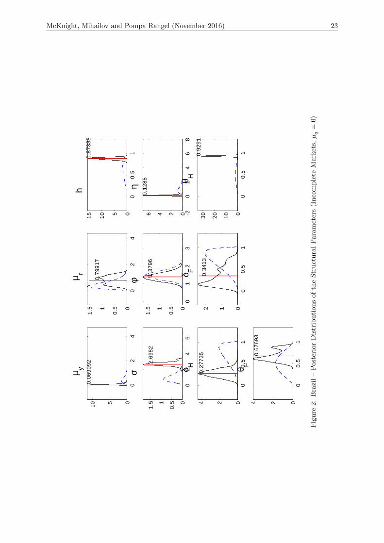
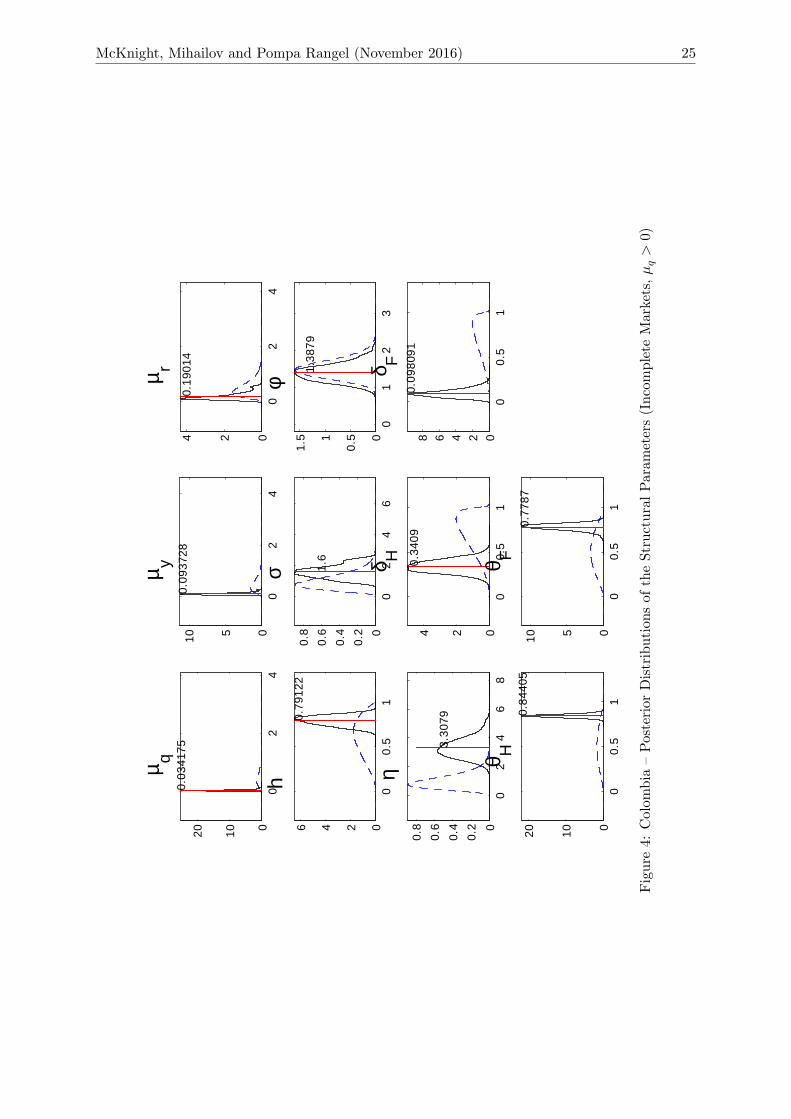
bank preferences obtained under each model version. Figures 1—7 depict the estimated posterior
distributions for each structural parameter and tables 4—10 report the posterior estimates and
convergence diagnostics for both the structural parameters and the persistence and standard
deviations of the shocks.
4.1 Model Comparison, Posterior Shapes and Convergence Diagnostics
For each country, Table 3 compares selected characteristics of the Bayesian RWMH-MCMC
estimation for the two model versions, µq > 0 and µq = 0. Comparison of the marginal
likelihoods reported in Table 3 suggests that the central banks of Chile, Mexico and Peru are
19The pseudo-code for this popular algorithm is detailed in Appendix B of Kam et al. (2009).20These values correspond to the average quarterly share (in our whole sample, 1999:1-2014:4) of real imports
of goods and services in real consumption by country. Since direct information for the latter ratio is usually notreleased in statistical publications, we obtained it indirectly, by the ratio of the average quarterly share of realimports of goods and services in GDP to the average quarterly share of real consumption in real GDP.21Using GMM, Selaive and Tuesta (2003 a, b) estimate χ to be in the range of 0.004 and 0.071 for a sample of
OECD countries.

What Do Latin American Inflation Targeters Care About? 12
explicitly concerned with stabilizing the real exchange rate. In the case of Brazil and Colombia,
the results suggest that the model µq = 0 is a better fit of the data in terms of having a higher
marginal likelihood.22 For the µq > 0 model version, with the exception of Brazil where the
acceptance rate is low, the acceptance rates obtained for Chile, Colombia, Mexico, and Peru all
fall within conventional range.23
For each model version, Table 3 also summarizes the parameter estimates associated with the
loss function of each central bank. By inspection, while there is significant heterogeneity in terms
of the specific parameter weights estimated for each country, three main conclusions arise. First,
there is significant evidence that all five central banks, with a possible exception of Colombia,
are concerned about smoothing the nominal interest rate. In particular, relative to the weight
of inflation stabilization (normalized at 1), we find that Brazil (0.8 or 1.06 depending on the
model version) and Peru (1.6) place very high weights on interest rate smoothing. Colombia is
found to have the lowest weight in both model versions (0.19 or 0.05). For the three countries
concerned about real exchange rate volatility (i.e., where the µq > 0 model version is preferable
in terms of marginal likelihoods), the estimates for Chile (0.11), and Peru (0.06) yield low
weights suggesting the low importance of real exchange rate stabilization in these countries. In
stark contrast, Mexico assigns a significant weight to real exchange rate stabilization (nearly
half of that to inflation stabilization, which is greater than interest rate smoothing (0.38) and
output gap stabilization (0.3). Third, while Brazil, Colombia, and Peru show little concern for
output gap stabilization, Chile (0.24) and Mexico (0.3) place a sizeable weight on it. Overall,
there is evidence to suggest that the central banks of Brazil, Colombia, and Peru implement a
strict inflation targeting policy with small weights assigned to real exchange rate stabilization
and output gap stabilization, whereas the central banks of Chile and Mexico appear to be more
flexible in terms of their inflation targeting preferences.
Figures 1—7 show both the assumed prior (dashed curve) and the estimated posterior (solid
curve) distributions (also indicating the posterior mean by the vertical line) for each structural
parameter for the five LAIT economies. For Brazil and Colombia we report both model versions
in the figures that depict the posterior distributions, whereas for the remaining three LAIT
countries we only report the µq > 0 case.24 By inspection, the posterior distributions are
generally unimodal and nicely shaped in most cases.
Tables 4—10 report the posterior mean and standard deviation estimates, the 95% confidence
sets for the posterior estimates, and selected diagnostic tests for MCMC convergence. As before,
for Brazil and Colombia we report both model versions in the tables and for the remaining
three LAIT countries we only report the µq > 0 case.25 In these tables, NSE stands for
the numerical standard error, which approximates the true posterior moment as proposed by
Geweke (1992). The NSE reported for each country uses an 8% autocovariance tapered estimate.
The G p-values report the p-value associated with Geweke’s (1992) chi-squared convergence
22This finding is further corroborated by the posterior densities reported in Table 3, which are very close tozero for Brazil and Colombia in the µq > 0 version of the model.23The Bayesian literature has no recommendation for a single value of an “optimal”acceptance rate. Common
practice considers the range from about 20% to 50% to be the most reliable (see, e.g., Koop, 2006, or Herbst andSchorfheide, 2016).24Results for all model versions for each country are available upon request.25Results for the µq = 0 model version are available upon request.

McKnight, Mihailov and Pompa Rangel (November 2016) 13
test.26 The last column of tables 4—10 reports the Brooks-Gelman (B-G) univariate shrink
factor proposed by Gelman and Rubin (1992) and extended by Brooks and Gelman (1998).27
By inspection of tables 4—10, we can conclude that our estimation results are overall satisfactory.
The reported convergence test statistics for the estimated parameters indicate that in general
the latter converge to an invariant distribution.28 There are few exceptions, however, where
both the Geweke chi-squared convergence test and the univariate shrink B-G factor both agree
on problems with convergence: δF for Brazil (for the µq = 0 model); ρq for Chile; σ, θF , σFand σs for Colombia (for the µq = 0 model); σH , σF , σa and σs for Mexico; σH and σπ∗ for
Peru.29
4.2 Estimated Structural Parameters Influencing the Endogenous Propaga-tion
We now check if the estimated key structural parameters are economically plausible and how
they compare to analogous earlier estimates.
We obtain estimates for habit persistence that are broadly consistent with the literature:
posterior mean of 0.87 for Brazil and 0.75 for Colombia for the preferred model version in the
case of these two counties (µq = 0), and of 0.77 for Chile and 0.92 for Mexico for the preferred
µq > 0 version. Peru, however, is an exception, with a low estimated habit persistence of 0.26.
Our estimates of the coeffi cient of relative risk aversion vary considerably across the five LAIT
countries: 0.97 in Chile and Mexico, 1.48 in Colombia and 2.7 in Brazil. Peru is again an
exception, with extremely low degree of relative risk aversion, 0.07. The inverse of the Frish
elasticity of labor supply is estimated within the usual range, 1.38 in Brazil, 1.46 in Chile, 1.36
in Colombia, 1.45 in Mexico, and 1.80 in Peru. With the exception of Peru, the estimated
elasticity of substitution between home and foreign goods is (roughly) within the typical range
of estimates found in the empirical literature of 0.1—2.0 (see, for example, Corsetti et al., 2008):
1.3 for Brazil, 1.72 for Chile, 2.89 for Colombia and 2.19 for Mexico.
The degree of domestic-output versus import price stickiness is estimated at 0.93 versus 0.68
for Brazil; 0.78 in both sectors for Chile; 0.80 versus 0.70 for Colombia; 0.97 versus 0.96 for
Mexico; and 0.26 versus 0.63 for Peru; Kam et al. (2009) find for all their sample countries a
consistently higher degree of price stickiness for domestic output relative to imported goods.
We find little difference in the estimates of price stickiness across sectors for Chile and Mexico,
whereas in Peru imported price stickiness is over twice higher in the imported sector. While
there is evidence of a high degree of sticky prices in the domestic economy for Brazil, Colombia,
Chile and Mexico, prices are much more flexible in Peru. The backward-lookingness of the
NKPC for home prices versus that for import prices is estimated at 0.28 versus 0.34 in Brazil,
26 If the Markov chain of draws has converged to a stable distribution, one would expect the means from thetwo halves of the generated sample to be statistically indistinguishable. The null hypothesis of the test is thatthe means are equal. Thus, a low p-value may indicate some evidence of problems in convergence.27This test runs the chain two or more times from a widely-dispersed starting point to see if the Markov
chain always converges to the same value. Commonly, a B-G factor below 1.1 is considered as little evidence ofdispersion (see, e.g., Gelman et al., 2004).28The MCMC diagnostics figures illustrating the convergence results discussed here are available upon request.29Note that Kam et al. (2009) report similar problems for some of the parameters we enumerated for Australia,
Canada, and New Zealand using a complete asset markets model.

What Do Latin American Inflation Targeters Care About? 14
0.24 versus 0.21 in Chile, 0.42 versus 0.15 in Colombia, 0.72 versus 0.38 in Peru, and 0.77
versus 0.65 in Mexico. For all five LAIT economies except Brazil, our findings reveal that
backward-lookingness in the NKPC is higher in domestic versus imported price inflation.
4.3 Estimated Persistence and Volatility of the Latent Exogenous ShockProcesses
We now turn to the sources of exogenous fluctuations in the LAIT economies, presenting our
set of estimates for persistence and volatility of the structural shock processes we included in
our model.30
As it was thus far, the estimated persistence of the exogenous shock processes reveals some
common features as well as some country specificity. To start with the persistence parameter
of the technology shock, its posterior mean is as follows: Brazil 0.98, Chile 0.46, Colombia 0.64,
Mexico 0.51 and Peru 0.89. The estimated (posterior mean) persistence of the risk premium
shock is, respectively: Brazil 0.80, Chile 0.86, Colombia 0.91, Mexico 0.99 and Peru 0.72; that
of the ToT shock is: Brazil 0.99, Chile 0.96, Colombia 0.65, Mexico 0.24 and Peru 0.44; and
the persistence of the preference shock is: Brazil 0.37, Chile 0.04, Colombia 0.04, Mexico 0.04,
Peru 0.11. Across all five LAIT economies, the most persistent shock appears to be the risk
premium shock, yet it does not dominate the persistence of some among the other shocks in
each individual country. Overall, the least persistent shock in all five LAIT economies is the
preference shock.
Looking now at the estimated volatility (measured by the posterior mean of the standard
deviation) of the exogenous shock processes, we could summarize the following findings. The
preference shock and the risk premium shock are among the most volatile in all countries except
Peru, where the terms of trade shock is the most volatile. With the exception of Brazil, the
terms of trade shock is of a comparable magnitude. Only in Mexico the technology shock plays
a role in driving volatility (but is not precisely estimated in terms of the diagnostics). For
Brazil, the cost-push shock in the imported goods sector appears to matter too, while for Peru
it is the cost-push shock in the domestic economy and the foreign inflation shock that come out
as sizable as well. Our estimates therefore show the importance in generating volatility of the
preference shock, which we incorporated in the SOE model with incomplete asset markets as
another realistic feature of the LAIT countries.
4.4 Complete versus Incomplete International Financial Markets
We now consider the role played by the assumption of incomplete international financial markets.
More precisely, we investigate the sensitivity of our results for the estimated policy parameters
to the asset market structure. We do this by reestimating the model under the alternative
assumption of complete asset markets employed in the closely-related study of Kam et al.
(2009).31 Specifically, we follow Kam et al. (2009) in estimating the complete asset markets
30The prior and posterior figures per country, illustrating the results discussed in the present subsection, areavailable upon request.31Palma and Portugal (2014) estimate the model of Kam et al. (2009) using Brazilian quarterly data (2000-
2013).

McKnight, Mihailov and Pompa Rangel (November 2016) 15
model using 9 observables (as the variable dt is now redundant) and 9 shocks (as the preference
shock εg,t is now omitted). The key difference is that complete asset markets implies perfect risk
sharing such that the real exchange rate equals the marginal rate of substitution in consumption
across countries. Incomplete international financial markets breaks this link (see Chari et al.,
2002, and Rabanal and Tuesta, 2010).
Table 11 summarizes the posterior mean and standard deviation for the central bank prefer-
ences for the two model versions, µq > 0 and µq = 0, estimated under complete asset markets.32
In stark contrast with the results reported in Table 3 under incomplete asset markets, we find
the following key differences. First, comparing the two model versions we now find for Peru the
model µq = 0 to be a better fit of the data (and not for Brazil and Colombia as under incom-
plete asset markets). Moreover, under complete asset markets both the central banks of Brazil33
and Chile assign a sizeable weight (0.31) to real exchange rate stabilization, whereas Mexico,
the only country to do so under incomplete asset markets, does not. Second, under complete
asset markets Brazil (0.73) and Colombia (0.51) are concerned about output gap stabilization,
instead of Chile and Mexico as under incomplete markets. Overall the central banks of Mexico
and Peru appear to implement a strict inflation targeting policy if the model is estimated under
complete asset markets, whereas Brazil, Colombia and Peru follow the same policy under in-
complete asset markets. While the major similarity between the two asset market structures is
the significant role of interest rate smoothing uncovered for all 5 LAIT central banks, the rank-
ing of the central bank target weights changes, except for Colombia, according to the assumed
structure of international financial markets.
The above exercise highlights the sensitivity of the Bayesian estimates for the central bank
policy weights to the assumption of international asset markets (in)completeness. Similar to
Rabanal and Tuesta (2010), we find that complete asset markets increase the degree of model
misspecification and distort significantly the Bayesian estimates, in particular the reported
policy parameters. For example, under incomplete asset markets we find no evidence that the
central bank of Brazil engages in real exchange rate and output stabilization, whereas for the
central bank of Mexico we find clear evidence of such concern. By contrast, under compete
asset markets these conclusions are reversed. In so far that incomplete asset markets are a more
realistic assumption, especially for developing countries, our analysis emphasizes the dangers
of using the common complete asset markets assumption in Bayesian estimation, in our case
focusing on uncovering central bank preferences.
5 Conclusions
The objective of this paper was to uncover and compare the central bank preferences of the
big five LAIT countries using Bayesian estimation. We employed a medium-scale New Key-
nesian small open economy model that assumed incomplete international asset markets and
imperfect ERPT. Optimal monetary policy was modeled under discretion, where the central
32The prior and posterior figures per country, illustrating the results discussed in the present subsection, areavailable upon request.33This is consistent with the findings of Palma and Portugal (2014) for the same model but a different sample.
However, they find a lower weight for output gap stabilization and a higher weight for interest rate inertia.

What Do Latin American Inflation Targeters Care About? 16
bank minimized an intertemporal quadratic loss function with four policy objectives: inflation
control, output gap stabilization, real exchange rate volatility reduction and nominal interest
rate smoothing. The weight attributed to each policy objective, which depends on the country-
specific institutional preferences of each central bank, was represented in terms of Bayesian
posterior distributions and convergence diagnostics.
The key insights of our analysis can be summarized as follows. The five LAIT economies we
considered seem to fall broadly into two groups. The first group consists of Brazil, Colombia and
Peru whose priority targets are to stabilize inflation with a significant degree of nominal interest
rate smoothing, consistent with strict IT. The second group, Chile and Mexico, has broader
policy objectives: both central banks additionally care about output gap stabilization, consistent
with flexible IT; only Mexico further assigns a sizeable weight to reducing real exchange rate
volatility. We also estimated the key structural parameters and the exogenous shocks. Our
Bayesian estimates reveal that three of the ten considered shocks drive the fluctuations in the
LAIT economies: the risk premium shock, the terms of trade shock and the preference shock.
We test the sensitivity of our results to the alternative assumption of complete asset markets
and find that a number of our key policy conclusions are now reversed. This suggests that
the degree of model misspecification depends on the asset market structure, highlighting the
limitations of employing the assumption of complete asset markets in Bayesian estimation,
especially when the aim is to uncover central bank preferences.
This work can be improved along various dimensions. It could be possible that preferences
were not constant over this period. Personalities of governors, in addition to the legal mandate
of the institution itself, could also shape the preferences of the central bank. For future research,
it would therefore be interesting to study separate subperiods in the institutional history or in
governor terms of offi ce within a central bank, and compare across such subperiods the estimated
policy preference parameters.

McKnight, Mihailov and Pompa Rangel (November 2016) 17
References
[1] Adolfson, M., Laseen, S., Lindé, J., Villani, M. (2007), “Bayesian Estimation of an Open
Economy DSGE Model with Incomplete Pass-through,” Journal of International Eco-
nomics 72, 481—511.
[2] An, S., and Schorfheide, F. (2007), “Bayesian Analysis of DSGE Models,”Econometric
Reviews 26, 211—219.
[3] Ball, C. P., and Reyes, J. (2004), “Inflation Targeting or Fear of Floating in Disguise: The
Case of Mexico,”International Journal of Finance & Economics 9, 49—69.
[4] Batini, N., and Laxton, D. (2007), “Under What Conditions Can Inflation Targeting Be
Adopted? The Experience of Emerging Markets,”in Mishkin, F., and Schmidt-Hebbel, K.
(eds.), Monetary Policy under Inflation Targeting. Central Bank of Chile, Santiago, 1—38.
[5] Benigno, G. and Benigno, P. (2003), “Price Stability in Open Economies,”Review of Eco-
nomic Studies 70, 743—764.
[6] Bernanke, B., and Mishkin, F. (1997), “Inflation Targeting: A New Framework for Mone-
tary Policy,”Journal of Economic Perspectives 11, 97—116.
[7] Brooks, S. P. and Gelman, A. (1998), “General Methods for Monitoring Convergence of
Iterative Simulations,”Journal of Computational and Graphical Statistics 7, 434—455.
[8] Brito, R., and Bystedt, B. (2010), “Inflation Targeting in Emerging Economies: Panel
Evidence,”Journal of Development Economics 91, 198—210.
[9] Calvo, G. (1983), “Staggered Prices in a Utility Maximizing Framework,”Journal of Mon-
etary Economics 12, 383—398.
[10] Capistrán, C., and Ramos-Francia, M. (2010), “Does Inflation Targeting Affect the Dis-
persion of Inflation Expectations?”Journal of Money, Credit and Banking 42, 113—134.
[11] Carare, A., and Stone, M. (2006), “Inflation Targeting Regimes,” European Economic
Review 50, 1297—1315.
[12] Carstens, A., and Werner, A. M. (2000), “Mexico’s Monetary Policy Framework Under
a Floating Exchange Rate Regime,”Money Affairs, Centro de Estudios Monetarios Lati-
noamericanos 0(2), 113—165.
[13] Castelnuovo, E., and Surico., P. (2004), “Model Uncertainty, Optimal Monetary Policy
and the Preferences of the Fed,”Scottish Journal of Political Economy 51, 105—126.
[14] Chari, V. V., Kehoe, P. J., and McGrattan, E. R. (2002), “Can Sticky Price Models
Generate Volatile and Persistent Real Exchange Rates?,”Review of Economic Studies 69,
533—563.
[15] Corsetti, G., Dedola, L., and Leduc, S. (2008), “International Risk Sharing and the Trans-
mission of Productivity Shocks”, Review of Economic Studies 75, 443—473.

What Do Latin American Inflation Targeters Care About? 18
[16] Del Negro, M., and Schorfheide, F. (2011), “Bayesian Macroeconometrics”, in J. Geweke,
G. Koop and H. van Dijk (eds.), The Oxford Handbook of Bayesian Econometrics, Oxford:
Oxford University Press (Ch. 7).
[17] DeJong, D., and Dave, C. (2011, 2nd ed.), Structural Macroeconometrics, Princeton, NJ,
and Oxford, England: Princeton University Press.
[18] Dennis, R. (2007), “Optimal Policy in Rational Expectations Models: New Solution Algo-
rithms,”Macroeconomic Dynamics 11, 31—55.
[19] Fernández-Villaverde, J., Guerron-Quintana, P. and Rubio-Ramírez, J. F. (2010) “The New
Macroeconometrics: A Bayesian Approach,”in A. O’Hagan and M. West (eds.), Handbook
of Applied Bayesian Analysis, Oxford: Oxford University Press.
[20] Fernández-Villaverde, J., Rubio-Ramírez, J. F., and Schorfheide, F. (in press), “Solution
and Estimation Methods for DSGE Models,” in J. Taylor and H. Uhlig (eds.), Handbook
of Macroeconomics, Volume 2, Elsevier.
[21] Galí, J. (2015, 2nd ed.), Monetary Policy, Inflation and the Business Cycle: An Introduc-
tion to the New Keynesian Framework and Its Applications, Princeton, NJ, and Oxford,
England: Princeton University Press.
[22] Galí, J., and Monacelli, T. (2005) “Monetary Policy and Exchange Rate Volatility in a
Small Open Economy,”Review of Economic Studies 72, 707—734.
[23] Gelfand, A. E. and Dey, D. K. (1994), “Bayesian Model Choice: Asymptotics and Exact
Calculations,”Journal of the Royal Statistical Society B 56, 501—514.
[24] Gelman, A., Carlin, J. B., Stern, H. S., Rubin, D. B. (2004, 2nd ed.), Bayesian Data
Analysis, Chapman & Hall/CRC.
[25] Gelman, A., and Rubin, D. B. (1992), “Inference from Iterative Simulation Using Multiple
Sequences,”Statistical Science 7, 457—511.
[26] Geweke, J. (1992), “Evaluating the Accuracy of Sampling-Based Approaches to Calculating
Posterior Moments,” in J. M. Bernardo, J. O. Berger, A. P. Dawid, and A. F. M. Smith
(eds.), Bayesian Statistics 4, Oxford, UK: Clarendon Press.
[27] Geweke, J. (1999), “Using Simulation Methods for Bayesian Econometric Models: Infer-
ence, Development, and Communication,”Econometric Reviews 18:1, 1-73.
[28] Goncalves, C., and Salles, J. (2008), “Inflation Targeting in Emerging Economies: What
Do the Data Say?”Journal of Development Economics 85, 312—318.
[29] Guerrón-Quintana, P., and Nason, J. M. (2012), “Bayesian Estimation of DSGE Models,”
FRB of Philadelphia Research Department Working Paper 12-4.
[30] Hammond, G. (2011) State of the Art of Inflation Targeting, Centre for Central Banking
Studies Handbook No. 29, London: Bank of England.
McKnight, Mihailov and Pompa Rangel (November 2016) 19
[31] Heathcote, J., and Perri, F. (2002), “Financial Autarky and International Business Cycles,”
Journal of Monetary Economics 49, 601—627.
[32] Herbst, Edward and Frank Schorfheide (2016), Bayesian Estimation of DSGE Models,
Princeton, NJ, and Oxford, England: Princeton University Press.
[33] Ilbas, P. (2010), “Estimation of Monetary Policy Preferences in a Forward-Looking Model:
A Bayesian Approach,”International Journal of Central Banking 6, 169—209.
[34] Ilbas, P. (2012), “Revealing the Preferences of the US Federal Reserve,”Journal of Applied
Econometrics 27, 440—473.
[35] International Monetary Fund (2012), Annual Report on Exchange Arrangements and Ex-
change Restrictions, IMF: Washington, DC.
[36] Jahan, S. (2012), “Inflation Targeting: Holding the Line,”Finance & Development (online:
updated on March 28, 2012).
[37] Justiniano, A., and Preston, B. (2010), “Monetary Policy and Uncertainty in an Empirical
Small Open-Economy Model,”Journal of Applied Econometrics 25, 93—128.
[38] Kam, T., Lees, K., and Liu, P. (2009), “Uncovering the Hit List for Small Inflation Tar-
geters: A Bayesian Structural Analysis,”Journal of Money, Credit and Banking 41, 583—
618.
[39] Koop, G. (2006, reprinted with corrections / 2003, 1st ed.), Bayesian Econometrics, Chich-
ester, England: John Wiley and Sons.
[40] Lee, W. (2011), “Comparative Case Studies of the Effects of Inflation Targeting in Emerging
Economies,”Oxford Economic Papers 63, 375—397.
[41] Lewis, K. K. (1995), “Puzzles in International Financial Markets”, in Grossman, G. and
Rogoff, K. (eds.), Handbook of International Economics, Elsevier, 1913—1971.
[42] Lin, S., and Ye, H. (2009), “Does Inflation Targeting Make a Difference in Developing
Countries?”Journal of Development Economics 89, 118—123.
[43] McKnight, S., and Mihailov, A. (2015), “Do Real Balance Effects Invalidate the Taylor
Principle in Closed and Open Economies?”Economica 82 (328), 938—975.
[44] Miao, J. (2014), Economic Dynamics in Discrete Time, Cambridge, MA, and London,
England: MIT Press.
[45] Mishkin, F. S., and Schmidt-Hebbel, K. (2001), “One Decade of Inflation Targeting in the
World: What Do We Know and What Do We Need to Know?”, NBER Working Paper
8397.
[46] Monacelli, T. (2005), “Monetary Policy in a Low Pass-Through Environment,”Journal of
Money, Credit and Banking 37, 1047—1066.

What Do Latin American Inflation Targeters Care About? 20
[47] Palma, A. A., and Portugal, M. S. (2014), “Preferences Of The Central Bank Of Brazil
Under The Inflation Targeting Regime: Estimation Using A DSGE Model For A Small
Open Economy,”Journal of Policy Modeling 36, 824—839.
[48] Rabanal, P. and Tuesta, V. (2010) “Euro-Dollar Real Exchange Rate Dynamics in an Es-
timated Two-Country Model: An Assessment,”Journal of Economic Dynamics & Control
34, 780—797.
[49] Roberts, G. O., Gelman, A., and Gilks, W. R. (1997), “Weak Convergence and Optimal
Scaling of Random Walk Metropolis Algorithms,”The Annals of Applied Probability 7, No.
1, 110—120.
[50] Raffo, A. (2010), “Technology Shocks: Novel Implications for International Business Cy-
cles,” International Finance Discussion Papers 992, Board of Governors of the Federal
Reserve System.
[51] Roger, S. (2010), “Inflation Targeting Turns 20,”Finance & Development 47, No. 1, 46—49.
[52] Schmitt-Grohe, S., and Uribe, M. (2003), “Closing Small Open Economy Models,”Journal
of International Economics 61, 163—185.
[53] Selaive, J., and Tuesta, V. (2003a), “Net Foreign Assets and Imperfect Pass-through: The
Consumption-Real Exchange Rate Anomaly,”Board of Governors of the Federal Reserve
System, International Finance Discussion Paper 764.
[54] Selaive, J., and Tuesta, V. (2003b), “Net Foreign Assets and Imperfect Financial Integra-
tion: An Empirical Approach,”Central Bank of Chile Working Paper 252.
[55] Smets, F., and Wouters, R. (2003), “An Estimated Dynamic Stochastic General Equilib-
rium Model of the Euro area,”Journal of the European Economic Association 1, 1123—1175.
[56] Smets F., andWouters, R. (2007), “Shocks and Frictions in US Business Cycles: A Bayesian
DSGE Approach,”American Economic Review 97, 586—606.
[57] Svensson, L. E. O. (1999), “Inflation Targeting as a Monetary Policy Rule,” Journal of
Monetary Economics 43, 607—654.
[58] Svensson, L. E. O. (2000), “Open-Economy Inflation Targeting,”Journal of International
Economics 50, 155—183.
[59] Taylor J. B. (1993), “Discretion versus Policy Rules in Practice,”Carnegie-Rochester Con-
ference Series on Public Policy 39, 195—214.
[60] Woodford, M. (2003), Interest Rates and Prices: Foundations of a Theory of Monetary
Policy, Princeton, NJ: Princeton University Press.

McKnight, Mihailov and Pompa Rangel (November 2016) 21
What Do Latin American Inflation Targeters Care About? 22
02
4020406080
0.00
8318
µ q
02
46
02460.
1064
9
µ y
02
40
0.51
1.5
1.05
73
µ r
00.
51
05100.
8638
7h
20
24
68
0
0.51
2.97
19
σ
01
23
0
0.51
1.5
1.34
96
φ
02
46
0240.
1390
8
η
00.
51
01230.
3189
1
δ H
00.
51
01230.
2260
7
δ F
00.
51
01020300.
9251
8
θ H
00.
51
0240.
7801
1
θ F
Figure1:Brazil—PosteriorDistributionsoftheStructuralParameters(IncompleteMarkets,µq>
0)
McKnight, Mihailov and Pompa Rangel (November 2016) 23
02
40510
0.06
9092
µ y
02
40
0.51
1.5
0.79
917
µ r
00.
51
0510150.
8733
8h
02
46
0
0.51
1.5
2.69
82
σ
01
23
0
0.51
1.5
1.37
96
φ
20
24
68
02460.
1285η
00.
51
0240.
2773
5
δ H
00.
51
0120.
3413
δ F
00.
51
01020300.
9291
θ H
00.
51
0240.
6769
3
θ F
Figure2:Brazil—PosteriorDistributionsoftheStructuralParameters(IncompleteMarkets,µq
=0)

What Do Latin American Inflation Targeters Care About? 24
02
40246
0.10
975
µ q
02
4012
0.26
568
µ y
02
40
0.51
1.5
0.45
333
µ r
00.
51
0240.
8136
6
h
02
46
0
0.51
0.71
933
σ
01
23
0
0.51
1.5
1.50
79
φ
02
46
0
0.51
1.22
5
η
00.
51
02460.
2631
1
δ H
00.
51
0240.
2363
2
δ F
00.
51
010200.
7746
9
θ H
00.
51
010200.
7731
6
θ F
Figure3:Chile—PosteriorDistributionsoftheStructuralParameters(IncompleteMarkets,µq>
0)
McKnight, Mihailov and Pompa Rangel (November 2016) 25
02
401020
0.03
4175
µ q
02
40510
0.09
3728
µ y
02
4024
0.19
014
µ r
00.
51
02460.
7912
2
h
02
46
00.
20.
40.
60.
81.
6
σ
01
23
0
0.51
1.5
1.38
79
φ
02
46
80
0.2
0.4
0.6
0.8
3.30
79
η
00.
51
0240.
3409
δ H
00.
51
024680.
0980
91
δ F
00.
51
010200.
8440
5
θ H
00.
51
05100.
7787
θ F
Figure4:Colombia—PosteriorDistributionsoftheStructuralParameters(IncompleteMarkets,µq>
0)

What Do Latin American Inflation Targeters Care About? 26
02
40102030
0.04
2714
µ y
02
4051015
0.04
7072
µ r
00.
51
05100.
7517
6h
02
46
0
0.51
1.5
1.47
55
σ
01
23
0
0.51
1.5
1.35
45
φ
02
46
00.
20.
40.
60.
8
2.89
31
η
00.
51
0240.
4244
7
δ H
00.
51
0240.
1530
1
δ F
00.
51
01020
0.80
442
θ H
00.
51
0510150.
6994
7
θ F
Figure5:Colombia—PosteriorDistributionsoftheStructuralParameters(IncompleteMarkets,µq
=0)

McKnight, Mihailov and Pompa Rangel (November 2016) 27
02
4012
0.48
203
µ q
02
40123
0.30
101
µ y
02
4012
0.38
073
µ r
00.
51
0510150.
9186
2h
20
24
68
0
0.51
1.5
0.97
409
σ
02
40
0.51
1.5
1.45
14
φ
02
46
00.
20.
40.
60.
8
2.18
58
η
00.
51
01230.
7706
5
δ H
00.
51
0120.
6462
4
δ F
00.
51
02040
0.96
922
θ H
00.
51
010200.
9644
2
θ F
Figure6:Mexico—PosteriorDistributionsoftheStructuralParameters(IncompleteMarkets,µq>
0)

What Do Latin American Inflation Targeters Care About? 28
02
4051015
0.06
212
µ q
01
23
02040600.
0105
58
µ y
02
40
0.51
1.5
1.59
6
µ r
00.
51
01230.
2629
h
02
46
05100.
0674
22
σ
01
23
0
0.51
1.5
1.80
39
φ
02
46
80
0.2
0.4
0.6
0.8
5.05
91
η
00.
51
0120.
7193
δ H
00.
51
0120.
3847
5
δ F
00.
51
0120.
2590
1
θ H
00.
51
0510
0.62
986
θ F
Figure7:Peru—PosteriorDistributionsoftheStructuralParameters(IncompleteMarkets,µq>
0)
McKnight, Mihailov and Pompa Rangel (November 2016) 29
Country Exchange Rate Year of IT Annual Inflation Average Quarterly InflationRegime (2012) Adoption at IT Adoption Inlation since IT Target (2012)
Brazil Floating 1999 3.3 6.6 4.5 ± 1Chile Free floating 1999 3.2 3.2 3 ± 1
Colombia Floating 1999 9.3 5.1 2 —4Guatemala Stabilized arrangement 2005 9.2 5.4 5 ± 1Mexico Free floating 2001 9.0 4.3 3 ± 1Peru Floating 2002 −0.1 2.9 2 ± 1
Note: Annual inflation is expressed in % per annum. Average quarterly inflation is computed fromthe first quarter of the year following IT adoption through the last quarter of 2014, and is expressedas % per annum. The exchange-rate regime classification is taken from IMF (2012). The inflationtarget is extracted from Jahan (2012).
Table 1: The 6 Latin American Inflation Targeters: Some Basic Facts

What Do Latin American Inflation Targeters Care About? 30
Parameters Description Prior pdf Prior Mean Prior SD
Structural Parameters
h degree of habit persistence B 0.6 0.2
σ inverse of elasticity of intertemporal substitution in consumption Γ 1.0 0.5
φ inverse of Frish elasticity of intertemporal labor supply Γ 1.5 0.25
η elasticity of substitution between home and foreign goods Γ 1.0 0.5
δH degree of indexation in domestic-output markets B 0.7 0.2
δF degree of indexation in imported-goods markets B 0.7 0.2
θH degree of inflation persistence in domestic-output markets B 0.5 0.2
θF degree of inflation persistence in imported-goods markets B 0.5 0.2
a1 degree of persistence in foreign inflation B 0.5 0.2
b2 degree of persistence in foreign output B 0.5 0.2
c3 degree of persistence in foreign interest rate B 0.5 0.2
ρa degree of persistence in technology shock B 0.5 0.2
ρq degree of persistence in risk premium shock B 0.9 0.2
ρs degree of persistence in terms of trade shock B 0.25 0.2
ρg degree of persistence of preference shock B 0.5 0.2
Relative Policy Target Weights
µq real exchange rate stabilization Γ 0.5 0.3
µy output gap stabilization Γ 0.5 0.3
µr interest rate smoothing Γ 0.5 0.3
Standard Deviation of Shock Innovations
σH domestic-output cost-push shock Inverse Γ 0.5 0.25
σF imported-goods cost-push shock Inverse Γ 0.5 0.25
σa technology shock Inverse Γ 1.0 0.4
σq risk premium shock Inverse Γ 2.0 0.5
σs terms of trade shock Inverse Γ 1.0 0.4
σπ∗ foreign inflation shock Inverse Γ 1.0 0.4
σy∗ foreign output shock Inverse Γ 1.0 0.4
σr∗ foreign interest rate shock Inverse Γ 1.0 0.4
σr interest rate shock Inverse Γ 1.0 0.4
σg preference shock Inverse Γ 1.0 0.4
Note: Parameters calibrated to a value common to all countries: β = 0.99; χ = 0.05. The parameter α is calibrated toa country-specific value. For the µq= 0 model version, the prior and posterior distributions are degenerate at zero.
Table 2: Prior Distributions

McKnight, Mihailov and Pompa Rangel (November 2016) 31
µq> 0 µq= 0
Brazil (2004—2014)
Marginal Likelihood -1778.7 -1766.7
Acceptance Rate (%) 6.94 9.24
Indeterminacy Rate (%) 24.15 24.08
Invalid Likelihood Rate (%) 0.001208 0.000200
µq 0.01 (0.01) 0
µy 0.11 (0.11) 0.07 (0.07)
µr 1.06 (0.26) 0.80 (0.31)
Chile (2002—2014)
Marginal Likelihood -1921.3 -1923.1
Acceptance Rate (%) 25.79 33.38
Indeterminacy Rate (%) 5.57 0.79
Invalid Likelihood Rate (%) 0.000273 0.001550
µq 0.11 (0.05) 0
µy 0.24 (0.10) 0.08 (0.04)
µr 0.51 (0.20) 0.25 (0.17)
Colombia (2003—2014)
Marginal Likelihood -1799.3 -1793.0
Acceptance Rate (%) 20.31 5.54
Indeterminacy Rate (%) 5.10 7.03
Invalid Likelihood Rate (%) 0.000255 0.000350
µq 0.03 (0.02) 0
µy 0.09 (0.04) 0.043 (0.014)
µr 0.19 (0.14) 0.047 (0.027)
Mexico (2002—2014)
Marginal Likelihood -1759.6 -1788.9
Acceptance Rate (%) 31.73 9.82
Indeterminacy Rate (%) 7.76 14.84
Invalid Likelihood Rate (%) 0.000388 0.007450
µq 0.48 (0.20) 0
µy 0.30 (0.14) 0.024 (0.01)
µr 0.38 (0.18) 1.50 (0.53)
Peru (2005—2014)
Marginal Likelihood -1610.1 -1700.7
Acceptance Rate (%) 37.32 3.41
Indeterminacy Rate (%) 0.11 32.06
Invalid Likelihood Rate (%) 0.000006 0.000250
µq 0.06 (0.03) 0
µy 0.01 (0.01) 0.006 (0.005)
µr 1.60 (0.46) 0.037 (0.029)
Note: Estimates of the policy weights (relative to that of inflation, 1), µi with i = {q, y, r},report the posterior mean, with the posterior standard deviation in parentheses.
Table 3: Model Comparison and Estimated Policy Weights

What Do Latin American Inflation Targeters Care About? 32
Parameters Post Mean Post SD 2.5% 97.5% NSE (8%) G p-value B-GFStructural Parameters
h 0.86 0.03 0.19 0.93 0.01 0.11 1.03σ 2.97 0.35 0.27 2.19 0.09 0.49 1.01φ 1.35 0.24 1.05 2.03 0.02 0.07 1.01η 0.14 0.07 0.27 2.19 0.01 0.09 1.03δH 0.32 0.10 0.25 0.98 0.01 0.67 1.00δF 0.23 0.13 0.25 0.98 0.02 0.12 1.04θH 0.93 0.01 0.13 0.87 0.00 0.13 1.01θF 0.78 0.10 0.13 0.87 0.02 0.46 1.01a1 0.63 0.12 0.19 0.96 0.01 0.86 1.00b2 0.82 0.06 0.19 0.96 0.00 0.08 1.00c3 0.99 0.01 0.19 0.96 0.00 0.37 1.00ρa 0.99 0.01 0.13 0.87 0.00 0.72 1.00ρq 0.89 0.21 0.23 1.00 0.05 0.29 1.02ρs 0.99 0.01 0.01 0.72 0.00 0.51 1.00ρg 0.38 0.05 0.13 0.87 0.00 0.64 1.00
Relative Policy Target Weightsµq 0.01 0.01 0.09 1.24 0.00 0.01 1.05µy 0.11 0.11 0.09 1.24 0.02 0.02 1.09µr 1.06 0.26 0.09 1.24 0.06 0.45 1.01
Standard Deviation of Shock InnovationsσH 2.07 1.31 0.91 7.33 0.31 0.00 1.25σF 3.99 3.48 0.91 7.34 0.94 0.00 2.11σa 5.18 1.87 0.52 2.66 0.45 0.04 1.07σq 23.73 1.16 0.32 0.87 0.25 0.83 1.00σs 13.39 2.88 0.52 2.66 0.76 0.25 1.02σπ∗ 0.51 0.15 0.52 2.65 0.01 0.06 1.01σy∗ 5.83 1.01 0.52 2.65 0.19 0.71 1.00σr∗ 0.28 0.03 0.52 2.66 0.00 0.04 1.00σr 0.58 0.07 0.52 2.66 0.00 0.74 1.00σg 24.80 0.17 0.52 2.66 0.02 0.69 1.00
Note: Calibrated parameters: β = 0.99; χ = 0.05; α = 0.20.
Table 4: Brazil: Posterior Parameters and Convergence Diagnostics (µq > 0)

McKnight, Mihailov and Pompa Rangel (November 2016) 33
Parameters Post Mean Post SD 2.5% 97.5% NSE (8%) G p-value B-GFStructural Parameters
h 0.87 0.03 0.19 0.93 0.00 0.46 1.00σ 2.70 0.26 0.27 2.19 0.05 0.46 1.01φ 1.38 0.23 1.05 2.03 0.01 0.16 1.00η 0.13 0.07 0.27 2.20 0.01 0.99 1.00δH 0.28 0.09 0.25 0.98 0.01 0.72 1.00δF 0.34 0.21 0.25 0.98 0.05 0.00 1.14θH 0.93 0.01 0.13 0.87 0.00 0.38 1.01θF 0.68 0.12 0.13 0.87 0.03 0.15 1.03a1 0.66 0.12 0.19 0.96 0.01 0.15 1.00b2 0.82 0.06 0.19 0.96 0.00 0.78 1.00c3 0.98 0.01 0.19 0.96 0.00 0.43 1.00ρa 0.98 0.01 0.13 0.87 0.00 0.02 1.02ρq 0.80 0.28 0.23 1.00 0.06 0.32 1.02ρs 0.99 0.01 0.01 0.73 0.00 0.00 1.03ρg 0.37 0.05 0.13 0.87 0.00 0.45 1.00
Relative Policy Target Weightsµy 0.07 0.07 0.09 1.24 0.01 0.04 1.05µr 0.80 0.31 0.10 1.23 0.07 0.79 1.00
Standard Deviation of Shock InnovationsσH 1.71 1.32 0.91 7.37 0.27 0.11 1.04σF 16.91 1.97 0.92 7.37 0.49 0.09 1.05σa 4.29 1.70 0.52 2.66 0.42 0.35 1.02σq 23.47 1.21 0.32 0.88 0.24 0.00 1.26σs 10.06 2.43 0.52 2.66 0.61 0.62 1.01σπ∗ 0.50 0.15 0.52 2.66 0.01 0.45 1.00σy∗ 5.14 0.88 0.52 2.66 0.15 0.16 1.03σr∗ 0.27 0.04 0.52 2.67 0.00 0.48 1.00σr 0.58 0.07 0.52 2.66 0.00 0.52 1.00σg 24.81 0.19 0.52 2.66 0.01 0.50 1.00
Note: Calibrated parameters: β = 0.99; χ = 0.05; α = 0.20.
Table 5: Brazil: Posterior Parameters and Convergence Diagnostics (µq = 0)

What Do Latin American Inflation Targeters Care About? 34
Parameters Post Mean Post SD 2.5% 97.5% NSE (8%) G p-value B-GFStructural Parameters
h 0.77 0.05 0.19 0.93 0.01 0.08 1.04σ 0.97 0.26 0.27 2.19 0.06 0.02 1.10φ 1.46 0.24 1.05 2.03 0.02 0.75 1.00η 1.72 0.66 0.27 2.19 0.12 0.82 1.00δH 0.24 0.05 0.25 0.98 0.01 0.30 1.01δF 0.21 0.06 0.25 0.98 0.01 0.52 1.00θH 0.78 0.02 0.13 0.87 0.00 0.06 1.01θF 0.78 0.02 0.13 0.87 0.00 0.30 1.00a1 0.50 0.11 0.19 0.96 0.00 0.58 1.00b2 0.85 0.07 0.19 0.96 0.00 0.11 1.00c3 0.99 0.02 0.19 0.96 0.00 0.14 1.00ρa 0.46 0.14 0.13 0.87 0.02 0.93 1.00ρq 0.86 0.25 0.24 1.00 0.06 0.01 1.14ρs 0.96 0.03 0.01 0.72 0.00 0.69 1.00ρg 0.04 0.04 0.13 0.87 0.00 0.67 1.00
Relative Policy Target Weightsµq 0.10 0.05 0.09 1.24 0.00 0.30 1.01µy 0.20 0.08 0.09 1.24 0.01 0.05 1.04µr 0.67 0.24 0.09 1.24 0.05 0.33 1.02
Standard Deviation of Shock InnovationsσH 1.35 0.68 0.91 7.33 0.11 0.36 1.01σF 1.79 1.07 0.91 7.34 0.22 0.05 1.06σa 1.34 0.69 0.52 2.66 0.09 0.42 1.01σq 23.76 0.92 0.32 0.87 0.17 0.14 1.03σs 24.60 0.35 0.52 2.65 0.04 0.43 1.01σπ∗ 2.37 0.85 0.52 2.65 0.18 0.09 1.04σy∗ 12.60 1.27 0.52 2.66 0.28 0.95 1.00σr∗ 0.25 0.03 0.52 2.66 0.00 0.62 1.00σr 0.62 0.07 0.52 2.66 0.00 0.35 1.00σg 24.52 0.44 0.52 2.66 0.05 0.21 1.02
Note: Calibrated parameters: β = 0.99; χ = 0.05; α = 0.51.
Table 6: Chile: Posterior Parameters and Convergence Diagnostics (µq > 0)

McKnight, Mihailov and Pompa Rangel (November 2016) 35
Parameters Post Mean Post SD 2.5% 97.5% NSE (8%) G p-value B-GFStructural Parameters
h 0.79 0.05 0.19 0.93 0.01 0.03 1.07σ 1.60 0.41 0.27 2.19 0.10 0.00 1.24φ 1.39 0.23 1.05 2.03 0.01 0.39 1.00η 3.31 0.70 0.27 2.19 0.10 0.14 1.02δH 0.34 0.07 0.25 0.98 0.01 0.65 1.00δF 0.10 0.04 0.25 0.98 0.00 0.81 1.00θH 0.84 0.02 0.13 0.87 0.00 0.12 1.02θF 0.78 0.04 0.13 0.87 0.00 0.16 1.02a1 0.51 0.11 0.19 0.96 0.00 0.25 1.00b2 0.83 0.07 0.19 0.96 0.00 0.85 1.00c3 0.98 0.01 0.19 0.96 0.00 0.85 1.00ρa 0.76 0.08 0.13 0.87 0.02 0.00 1.10ρq 0.98 0.05 0.24 1.00 0.00 0.38 1.01ρs 0.89 0.07 0.01 0.72 0.01 0.04 1.04ρg 0.06 0.04 0.13 0.87 0.00 0.28 1.00
Relative Policy Target Weightsµq 0.03 0.02 0.09 1.23 0.00 0.00 1.08µy 0.09 0.04 0.09 1.24 0.01 0.00 1.06µr 0.19 0.14 0.09 1.24 0.02 0.00 1.19
Standard Deviation of Shock InnovationsσH 1.97 1.13 0.91 7.33 0.24 0.09 1.05σF 3.08 1.75 0.91 7.34 0.42 0.00 1.18σa 1.71 0.89 0.52 2.66 0.21 0.00 1.24σq 24.20 0.66 0.32 0.87 0.11 0.22 1.02σs 13.11 3.32 0.52 2.66 0.87 0.00 1.63σπ∗ 0.69 0.25 0.52 2.65 0.03 0.34 1.01σy∗ 6.91 1.12 0.52 2.66 0.21 0.21 1.03σr∗ 0.25 0.03 0.52 2.65 0.00 0.61 1.00σr 0.62 0.07 0.52 2.66 0.00 0.32 1.00σg 24.21 0.79 0.52 2.65 0.16 0.08 1.05
Note: Calibrated parameters: β = 0.99; χ = 0.05; α = 0.29.
Table 7: Colombia: Posterior Parameters and Convergence Diagnostics (µq > 0)
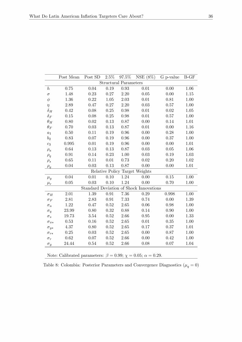
What Do Latin American Inflation Targeters Care About? 36
Post Mean Post SD 2.5% 97.5% NSE (8%) G p-value B-GFStructural Parameters
h 0.75 0.04 0.19 0.93 0.01 0.00 1.06σ 1.48 0.23 0.27 2.20 0.05 0.00 1.15φ 1.36 0.22 1.05 2.03 0.01 0.81 1.00η 2.89 0.47 0.27 2.20 0.03 0.57 1.00δH 0.42 0.08 0.25 0.98 0.01 0.02 1.05δF 0.15 0.08 0.25 0.98 0.01 0.57 1.00θH 0.80 0.02 0.13 0.87 0.00 0.14 1.01θF 0.70 0.03 0.13 0.87 0.01 0.00 1.16a1 0.50 0.11 0.19 0.96 0.00 0.28 1.00b2 0.83 0.07 0.19 0.96 0.00 0.37 1.00c3 0.995 0.01 0.19 0.96 0.00 0.00 1.01ρa 0.64 0.13 0.13 0.87 0.03 0.05 1.06ρq 0.91 0.14 0.23 1.00 0.03 0.19 1.03ρs 0.65 0.11 0.01 0.73 0.02 0.20 1.02ρg 0.04 0.03 0.13 0.87 0.00 0.00 1.01
Relative Policy Target Weightsµy 0.04 0.01 0.10 1.24 0.00 0.15 1.00µr 0.05 0.03 0.10 1.24 0.00 0.70 1.00
Standard Deviation of Shock InnovationsσH 2.01 1.39 0.91 7.36 0.29 0.998 1.00σF 2.81 2.83 0.91 7.33 0.74 0.00 1.39σa 1.22 0.47 0.52 2.65 0.06 0.98 1.00σq 23.99 0.80 0.32 0.88 0.14 0.90 1.00σs 19.73 3.54 0.52 2.66 0.95 0.00 1.33σπ∗ 0.53 0.16 0.52 2.65 0.01 0.35 1.00σy∗ 4.37 0.80 0.52 2.65 0.17 0.37 1.01σr∗ 0.25 0.03 0.52 2.65 0.00 0.87 1.00σr 0.62 0.07 0.52 2.66 0.00 0.42 1.00σg 24.44 0.54 0.52 2.66 0.08 0.07 1.04
Note: Calibrated parameters: β = 0.99; χ = 0.05; α = 0.29.
Table 8: Colombia: Posterior Parameters and Convergence Diagnostics (µq = 0)
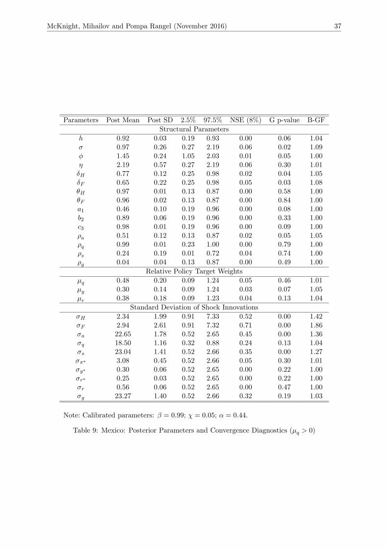
McKnight, Mihailov and Pompa Rangel (November 2016) 37
Parameters Post Mean Post SD 2.5% 97.5% NSE (8%) G p-value B-GFStructural Parameters
h 0.92 0.03 0.19 0.93 0.00 0.06 1.04σ 0.97 0.26 0.27 2.19 0.06 0.02 1.09φ 1.45 0.24 1.05 2.03 0.01 0.05 1.00η 2.19 0.57 0.27 2.19 0.06 0.30 1.01δH 0.77 0.12 0.25 0.98 0.02 0.04 1.05δF 0.65 0.22 0.25 0.98 0.05 0.03 1.08θH 0.97 0.01 0.13 0.87 0.00 0.58 1.00θF 0.96 0.02 0.13 0.87 0.00 0.84 1.00a1 0.46 0.10 0.19 0.96 0.00 0.08 1.00b2 0.89 0.06 0.19 0.96 0.00 0.33 1.00c3 0.98 0.01 0.19 0.96 0.00 0.09 1.00ρa 0.51 0.12 0.13 0.87 0.02 0.05 1.05ρq 0.99 0.01 0.23 1.00 0.00 0.79 1.00ρs 0.24 0.19 0.01 0.72 0.04 0.74 1.00ρg 0.04 0.04 0.13 0.87 0.00 0.49 1.00
Relative Policy Target Weightsµq 0.48 0.20 0.09 1.24 0.05 0.46 1.01µy 0.30 0.14 0.09 1.24 0.03 0.07 1.05µr 0.38 0.18 0.09 1.23 0.04 0.13 1.04
Standard Deviation of Shock InnovationsσH 2.34 1.99 0.91 7.33 0.52 0.00 1.42σF 2.94 2.61 0.91 7.32 0.71 0.00 1.86σa 22.65 1.78 0.52 2.65 0.45 0.00 1.36σq 18.50 1.16 0.32 0.88 0.24 0.13 1.04σs 23.04 1.41 0.52 2.66 0.35 0.00 1.27σπ∗ 3.08 0.45 0.52 2.66 0.05 0.30 1.01σy∗ 0.30 0.06 0.52 2.65 0.00 0.22 1.00σr∗ 0.25 0.03 0.52 2.65 0.00 0.22 1.00σr 0.56 0.06 0.52 2.65 0.00 0.47 1.00σg 23.27 1.40 0.52 2.66 0.32 0.19 1.03
Note: Calibrated parameters: β = 0.99; χ = 0.05; α = 0.44.
Table 9: Mexico: Posterior Parameters and Convergence Diagnostics (µq > 0)
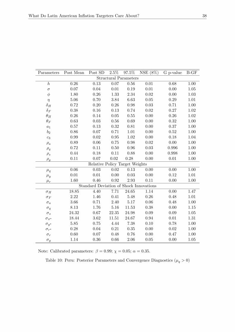
What Do Latin American Inflation Targeters Care About? 38
Parameters Post Mean Post SD 2.5% 97.5% NSE (8%) G p-value B-GFStructural Parameters
h 0.26 0.13 0.07 0.56 0.01 0.68 1.00σ 0.07 0.04 0.01 0.19 0.01 0.00 1.05φ 1.80 0.26 1.33 2.34 0.02 0.00 1.03η 5.06 0.70 3.84 6.63 0.05 0.29 1.01δH 0.72 0.20 0.26 0.98 0.03 0.71 1.00δF 0.38 0.16 0.13 0.74 0.02 0.27 1.02θH 0.26 0.14 0.05 0.55 0.00 0.26 1.02θF 0.63 0.03 0.56 0.69 0.00 0.32 1.00a1 0.57 0.13 0.32 0.81 0.00 0.37 1.00b2 0.86 0.07 0.71 1.01 0.00 0.52 1.00c3 0.99 0.02 0.95 1.02 0.00 0.18 1.04ρa 0.89 0.06 0.75 0.98 0.02 0.00 1.00ρq 0.72 0.11 0.50 0.96 0.03 0.996 1.00ρs 0.44 0.18 0.11 0.88 0.00 0.998 1.00ρg 0.11 0.07 0.02 0.28 0.00 0.01 1.00
Relative Policy Target Weightsµq 0.06 0.03 0.02 0.13 0.00 0.00 1.00µy 0.01 0.01 0.00 0.03 0.00 0.12 1.01µr 1.60 0.46 0.92 2.93 0.11 0.00 1.00
Standard Deviation of Shock InnovationsσH 18.85 4.40 7.71 24.65 1.14 0.00 1.47σF 2.22 1.46 0.41 5.48 0.26 0.48 1.01σa 3.66 0.71 2.40 5.17 0.06 0.48 1.00σq 8.13 1.76 5.16 11.53 0.38 0.00 1.15σs 24.32 0.67 22.35 24.98 0.09 0.09 1.05σπ∗ 18.44 3.62 11.51 24.67 0.94 0.01 1.31σy∗ 5.85 0.75 4.44 7.38 0.10 0.78 1.00σr∗ 0.28 0.04 0.21 0.35 0.00 0.02 1.00σr 0.60 0.07 0.48 0.76 0.00 0.47 1.00σg 1.14 0.36 0.66 2.06 0.05 0.00 1.05
Note: Calibrated parameters: β = 0.99; χ = 0.05; α = 0.35.
Table 10: Peru: Posterior Parameters and Convergence Diagnostics (µq > 0)

McKnight, Mihailov and Pompa Rangel (November 2016) 39
µq> 0 µq= 0
Brazil (2004—2014)
Marginal Likelihood -1431.5 -1469.8
Acceptance Rate (%) 12.93 8.24
Indeterminacy Rate (%) 4.72 18.16
Invalid Likelihood Rate (%) 2.247600 1.929550
µq 0.31 (0.12) 0
µy 0.73 (0.22) 0.78 (0.34)
µr 0.53 (0.30) 0.39 (0.18)
Chile (2002—2014)
Marginal Likelihood -1591.9 -1606.4
Acceptance Rate (%) 20.50 20.28
Indeterminacy Rate (%) 9.13 14.36
Invalid Likelihood Rate (%) 1.534950 0.679450
µq 0.31 (0.11) 0
µy 0.17 (0.09) 0.06 (0.04)
µr 1.14 (0.39) 1.08 (0.17)
Colombia (2003—2014)
Marginal Likelihood -1504.6 -1506.2
Acceptance Rate (%) 22.66 18.61
Indeterminacy Rate (%) 2.41 6.31
Invalid Likelihood Rate (%) 1.775850 1.896250
µq 0.13 (0.06) 0
µy 0.51 (0.22) 0.44 (0.19)
µr 0.54 (0.34) 0.47 (0.27)
Mexico (2002—2014)
Marginal Likelihood -1527.6 -1560.7
Acceptance Rate (%) 20.86 22.69
Indeterminacy Rate (%) 4.19 5.12
Invalid Likelihood Rate (%) 1.600200 2.042550
µq 0.06 (0.04) 0
µy 0.10 (0.05) 0.01 (0.01)
µr 0.43 (0.30) 1.29 (0.33)
Peru (2005—2014)
Marginal Likelihood -1437.1 -1399.8
Acceptance Rate (%) 29.18 15.97
Indeterminacy Rate (%) 6.67 1.14
Invalid Likelihood Rate (%) 1.018800 2.664300
µq 0.11 (0.07) 0
µy 0.62 (0.23) 0.03 (0.02)
µr 0.85 (0.26) 1.78 (0.48)
Note: Estimates of the policy weights (relative to that of inflation, 1), µi with i = {q, y, r},report the posterior mean, with the posterior standard deviation in parentheses.
Table 11: Model Comparison under Complete Asset Markets