What Do You Think Would Make You Happier?

What Do You Think You Would Choose?*

Daniel J. Benjamin Cornell University and NBER

Ori Heffetz Cornell University

Miles S. Kimball

University of Michigan and NBER

Alex Rees-Jones Cornell University

First Draft: July 26, 2010

This Draft: July 26, 2011

Abstract

Would people choose what they think would maximize their subjective well-being (SWB)? We

present survey respondents with hypothetical scenarios and elicit both choice and predicted SWB

rankings of two alternatives. While choice and predicted SWB rankings usually coincide in our

data, we find systematic reversals. We identify factors—such as predicted sense of purpose,

control over one’s life, family happiness, and social status—that help explain hypothetical choice

controlling for predicted SWB. We explore how our findings vary by SWB measure and by

scenario. Our results have implications regarding the use of SWB survey questions as a proxy for

utility.

JEL Classification: D03, D60

Keywords: happiness, life satisfaction, subjective well-being, hypothetical choice, utility

* A previous version of this paper circulated under the title “Do People Seek to Maximize Happiness? Evidence

from New Surveys.” We are extremely grateful to Dr. Robert Rees-Jones and his office staff for generously allowing

us to survey their patients and to Cornell’s Survey Research Institute for allowing us to put questions in the 2009

Cornell National Social Survey. We thank Gregory Besharov, John Ham, Benjamin Ho, Erzo F. P. Luttmer,

Michael McBride, Ted O’Donoghue, Matthew Rabin, Antonio Rangel, and Robert J. Willis for especially valuable

early comments and suggestions, as well as the editor and four anonymous referees for suggestions that substantially

improved the paper. We are grateful to participants at the CSIP Workshop on Happiness and the Economy, the

NBER Summer Institute, the Stanford Institute for Theoretical Economics (SITE), the Lausanne Workshop on

Redistribution and Well-Being, the Cornell Behavioral/Experimental Lab Meetings, and seminar audiences at

Cornell, Deakin, Syracuse, Wharton, Florida State, Bristol, Warwick, Dartmouth, Berkeley, Princeton, Penn,

RAND, and East Anglia for helpful comments. We thank Eric Bastine, Colin Chan, J.R. Cho, Kristen Cooper, Isabel

Fay, John Farragut, Geoffrey Fisher, Sean Garborg, Arjun Gokhale, Jesse Gould, Kailash Gupta, Han Jiang, Justin

Kang, June Kim, Nathan McMahon, Elliot Mandell, Cameron McConkey, Greg Muenzen, Desmond Ong, Mihir

Patel, John Schemitsch, Brian Scott, Abhishek Shah, James Sherman, Dennis Shiraev, Elizabeth Traux, Charles

Whittaker, Brehnen Wong, Meng Xue, and Muxin Yu for their research assistance. We thank the National Institute

on Aging (grant P01-AG026571/01) for financial support.

E-mail: db468@cornell.edu, oh33@cornell.edu, mkimball@umich.edu, arr34@cornell.edu.

2

All things considered, how satisfied are you with your life as a whole these days?

Taken all together, how would you say things are these days—would you say that you are

very happy, pretty happy, or not too happy?

Much of the time during the past week, you felt you were happy. Would you say yes or no?1

Economists increasingly use survey-based measures of subjective well-being (SWB) as

an empirical proxy for utility. In many applications, SWB data are used for testing or estimating

preference models, or for conducting welfare evaluations, in situations where these are difficult

to do credibly with choice-based revealed-preference methods. Examples include estimating the

negative externality from neighbors’ higher earnings (Erzo F.P. Luttmer, 2005), individuals’

tradeoff between inflation and unemployment (Rafael Di Tella, Robert J. MacCulloch, and

Andrew J. Oswald, 2003), and the effect of health status on the marginal utility of consumption

(Amy Finkelstein, Luttmer, and Matthew J. Notowidigdo, 2008). Such work often points out that

in addition to being readily available where choice-based methods might not be, SWB-based

proxies avoid the concern that choices may reflect systematically biased beliefs about their

consequences (e.g., George Loewenstein, Ted O’Donoghue, and Matthew Rabin, 2003; Daniel

T. Gilbert, 2006). It hence interprets SWB data as revealing what people would choose if they

were well-informed about the consequences of their choices for SWB, and uses SWB measures

to proxy for utility under the assumption that people make the choices they think would

maximize their SWB. This paper provides evidence for evaluating that assumption.

We pose a variety of hypothetical decision scenarios to three respondent populations: a

convenience sample of 1,066 adults, a representative sample of 1,000 adult Americans, and 633

students. Each scenario has two alternatives. For example, one scenario describes a choice

between a job that pays less but allows more sleep versus a job with higher pay and less sleep.

We ask respondents which alternative they think they would choose. We also ask them under

which alternative they anticipate greater SWB; we assess this “predicted SWB” using measures

based on each of the three commonly-used SWB questions posed in the epigraph above. We test

1 The first of these three questions is from the World Values Survey; similar questions appear in the Euro-Barometer

Survey, the European Social Survey, the German Socioeconomic Panel, and the Japanese Life in Nation survey. The

second question is from the U.S. General Social Survey; similar questions appear in the Euro-Barometer survey, the

National Survey of Families and Households, and the World Values Survey. The third question is from the

University of Michigan’s Survey of Consumers; similar questions appear in the Center of Epidemiologic Studies

Depression Scale, the Health and Retirement Study, and the Gallup-Healthways Well-Being Index.

3

whether these two rankings coincide.2 To the extent that they do not, we attempt to identify—by

eliciting predictions about other consequences of the choice alternatives—what else besides

predicted SWB explains respondents’ hypothetical choices, and to quantify the relative

contribution of predicted SWB and other factors in explaining these choices.

In designing our surveys, we made two methodological decisions that merit discussion.

First, while the purpose of our paper is to help relate choice behavior to SWB measures, those

measures are based on reports of respondents’ general levels of realized SWB, whereas our

survey questions elicit respondents’ predictions comparing the SWB consequences of specific

choices. To compare SWB rankings with choice rankings under the same information set and

beliefs, however, we must measure predictions about SWB because it is only predictions that are

available at the moment of choice. Moreover, to link SWB with choice, we must focus on the

SWB consequences of specific choices.

Second, while economists generally prefer data on incentivized choices, our choice data

consist of responses to questions about predicted choice in hypothetical scenarios. This is a

limitation of our approach because the two may not be the same.3 However, using hypothetical

scenarios allows us to address a much wider variety of relevant real-world choice situations. It

also allows us to have closely comparable survey measures of choice and SWB.4 For brevity,

hereafter we will sometimes omit the modifiers “predicted” and “hypothetical” when the context

makes it clear that by “choice” and “SWB” we refer to our survey questions.

We have two main results. First, we find that overall, respondents’ SWB predictions are a

powerful predictor of their choices. On average, SWB and choice coincide 83 percent of the time

in our data. We find that the strength of this relationship varies across choice situations, subject

populations, survey methods, questionnaire structure variations, and measures of SWB, with

2 In the terminology of Daniel Kahneman, Peter P. Wakker, and Rakesh K. Sarin (1997), our work can be viewed as

comparing “decision utility” (what people choose) with “predicted utility” (what people predict will make them

happier). We avoid these terms, however, because our “decisions” are hypothetical; and because we ask respondents

to predict their responses to common SWB survey questions, rather than the integral over time of their moment-by-

moment affect. 3 Although economists generally prefer data on incentivized choices, in some situations self-reports may be more

informative about preferences, e.g., when temptation, social pressure, or family bargaining might distort real-world

choices away from preferences. (As we mention below, our data are silent on which method best elicits preferences.) 4 The advantage in having closely comparable (survey-based) measures is that when we find discrepancies between

choice responses and SWB responses, these discrepancies can be attributed wholly to differences in question content

rather than at least partially to differences in how respondents react to the perceived realness of the consequences of

their response.

4

coincidence ranging from well below 50 percent to above 95 percent.

Our second main result is that discrepancies between choice and SWB rankings are

systematic. Moreover, we can indeed identify other factors that help explain respondents’

choices. As mentioned above, in addition to eliciting participants’ choices and predicted SWB, in

some surveys we also elicit their predictions regarding particular aspects of life other than their

own SWB. The aspects that systematically contribute most to explaining choice, controlling for

own SWB, are sense of purpose, control over life, family happiness, and social status. At the

same time, and in line with our first main result above, when we compare the predictive power of

own SWB to that of the other factors we measure, we find that across our scenarios, populations,

and methods, it is by far the single best predictor of choice.

We use a variety of survey versions and empirical approaches in order to test the

robustness of our main results to alternative interpretations. For example, while most of our data

are gathered by eliciting both choice and predicted SWB rankings from each respondent, in some

of our survey variations we elicit the two rankings far apart in the survey, or we elicit only

choice rankings from some participants and only SWB rankings from others. As another

example, we assess the impact of measurement error by administering the same survey twice

(weeks or months apart) to some of our respondents. While these different approaches affect our

point estimates and hence the relative importance of our two main results, both results appear to

be robust.

As steps toward providing practical, measure-specific and situation-specific guidance to

empirical researchers as to when the assumption that people’s choices maximize their predicted

SWB is a better or worse approximation, we analyze how our results differ across SWB

measures and across scenarios. Comparing SWB measures, we find that in our data, a “life

satisfaction” measure (modeled after the first question in the epigraph) is a better predictor of

choice than either of two “happiness” measures (modeled after the second and third questions in

the epigraph) that perform similarly to each other. Comparing scenarios, we find that in scenarios

constructed to resemble what our student respondents judge as representative of important

decisions in their lives, predicted SWB coincides least often with choice, and other factors add

relatively more explanatory power. We also find that in scenarios where one alternative offers

more money, respondents are systematically more likely to choose the money alternative than

they are likely to predict it will yield higher SWB. Under some conditions, this last finding

5

suggests that the increasingly common method of valuing non-market goods by comparing the

coefficients from a regression of SWB on income and on the amount of a good5 systematically

estimates a higher value than incentivized-choice-based methods of eliciting willingness-to-pay

(since the weight of money in predicted SWB understates its weight in choice).

Much previous research has studied the relationship between choice and happiness.6 Our

work is most closely related to experiments reported in Amos Tversky and Dale Griffin (1991),

Christopher H. Hsee (1999), and Hsee, Jiao Zhang, Fang Yu, and Yiheng Xi (2003) that use

methods similar to some of ours.7 However, because our goal is to provide guidance for

interpreting results from the empirical economics literature, our paper differs from these prior

papers in two fundamental ways. First, both our scenarios and our SWB measures are tailored to

be closely relevant to the economics literature. Thus, rather than primarily focusing on narrow

affective reactions to specific consumption experiences (e.g., the “enjoyment” of a sound

system), as in Hsee (1999) and Hsee et al. (2003), we purposefully model our measures on the

SWB questions asked in large-scale social surveys, and we focus on a range of scenarios that we

designed to be relevant to empirical work in economics as well as scenarios that are judged by

our respondents to represent important decisions in their lives. Second, crucially, we elicit

predictions about other valued aspects of the choice alternatives. Indeed, it has often been

observed that factors beyond one’s own happiness (in the narrow sense measured by standard

5 Recent examples have valued deaths in one’s family (Angus Deaton, Jane Fortson and Robert Tortora, 2010), the

social costs of terrorism (Bruno S. Frey, Simon Luechinger, and Alois Stutzer, 2009), and the social cost of floods

(Luechinger and Paul A. Raschky, 2009). 6 In a spirit similar to ours, Gary S. Becker and Luis Rayo (2008) propose (but do not pursue) empirical tests of

whether things other than happiness matter for preferences in empirically-relevant choice situations. Relatedly,

Ricardo Perez-Truglia (2010) tests empirically whether the utility function inferred from consumption choices is

distinguishable from the estimated happiness function over consumption. In contrast to our approach, these tests and

their interpretation are affected by whether individuals correctly predict the SWB consequences of their choices.

Our work is also related to a literature in philosophy that poses thought experiments in hypothetical scenarios in

order to demonstrate that people’s preferences encompass more than their own happiness (e.g., Robert Nozick,

1974, pp. 42-45), but that literature focuses on extreme situations, such as being hooked up to a machine that

guarantees happiness, and focuses on an abstract conception of happiness that is broader than empirical measures. 7 These papers find discrepancies between choice and predicted affective reactions, in hypothetical scenarios

carefully designed to test theories about why the two may differ. Tversky and Griffin (1991) theorize that payoff

levels are weighted more heavily in choice, while contrasts between payoffs and a reference point are weighted

more heavily in happiness judgments. Hsee (1999) and Hsee et al. (2003) theorize that when making choices,

individuals engage in “lay rationalism,” i.e., they mistakenly put too little weight on anticipated affect and too much

weight on “rationalistic” factors that include payoff levels as well as quantitatively-measured attributes. Our finding

that factors other than SWB help predict choice provides a different possible perspective on the evidence from these

earlier papers.

6

survey measures) may matter for choice.8 As far as we are aware, however, our work is the first

to quantitatively estimate the relative contribution of predicted SWB and these other factors in

explaining choice.

The rest of the paper is organized as follows. Section I discusses the survey design and

subject populations. Section II asks whether participants choose the alternative in our decision

scenarios that they predict will generate greater SWB. Section III asks whether aspects of life

other than SWB help predict choice, controlling for SWB, and compares the relative predictive

power of the factors that matter for choice. Section IV presents robustness analyses. Section V

characterizes the heterogeneity in choice-SWB concordance across SWB measures, scenarios,

and respondent characteristics. Section VI concludes and discusses other possible applications of

our methodology and implications of our findings. For example, while our paper focuses on

testing measures that are based on existing SWB survey questions, our methodology can be used

to explore whether alternative, novel questions could better explain choice. And while our data

cannot inform us regarding the best way to elicit preferences, if one assumes that hypothetical

choices reveal preferences, then our findings may imply that individuals do not exclusively seek

to maximize SWB as currently measured. The Appendix lists our decision scenarios. For longer

discussions, as well as detailed information on all survey instruments, pilots, robustness analyses,

and additional results, see our working paper, Daniel J. Benjamin, Ori Heffetz, Miles S. Kimball,

and Alex Rees-Jones (2010) with its Web Appendix (hereafter BHKR).

I. Survey Design

While our main evidence is based on 29 different survey versions, they all share a similar

core that consists of a sequence of hypothetical pairwise-choice scenarios. To illustrate, our

‘Scenario 1’ highlights a tradeoff between sleep and income. Followed by its SWB and choice

questions, it appears on one of our questionnaires as follows:

Say you have to decide between two new jobs. The jobs are exactly the same in almost every way, but have different work hours and pay different amounts. Option 1: A job paying $80,000 per year. The hours for this job are reasonable, and you would be able to get about 7.5 hours of sleep on the average work night.

8 For a few recent examples, see Ed Diener and Christie Scollon (2003), Loewenstein and Peter A. Ubel (2008, pp.

1801-1804), Hsee, Reid Hastie, and Jingqui Chen (2008, p. 239), and Marc Fleurbaey (2009).

7

Option 2: A job paying $140,000 per year. However, this job requires you to go to work at unusual hours, and you would only be able to sleep around 6 hours on the average work night.

Between these two options, taking all things together, which do you think would give you a happier life as a whole?

Option 1: Sleep more but earn less

Option 2: Sleep less but earn more

definitely happier

probably happier

possibly happier

possibly happier

probably happier

definitely happier

X X X X X X

Please circle one X in the line above

If you were limited to these two options, which do you think you would choose?

Option 1: Sleep more but earn less

Option 2: Sleep less but earn more

definitely choose

probably choose

possibly choose

possibly choose

probably choose

definitely choose

X X X X X X

Please circle one X in the line above

In within-subject questionnaires, respondents are asked both the SWB question and the

choice question above. In between-subjects questionnaires, respondents are asked only one of the

two questions.

I.A. Populations and Studies

We conducted surveys among 2,699 respondents from three populations: 1,066 patients

at a doctor’s waiting room in Denver who participated voluntarily; 1,000 adults who participated

by telephone in the 2009 Cornell National Social Survey (CNSS) and form a nationally

representative sample;9 and 633 Cornell students who were recruited on campus and participated

for pay or for course credit. The Denver and Cornell studies include both within-subject and

between-subjects survey variants, while the CNSS study is exclusively within-subject.

Table 1 summarizes the design details of these studies. It lists each study’s respondent

population, sample size, scenarios used (see I.B below), types of questions asked (see I.C below),

9 The CNSS is an annual survey conducted by Cornell University’s Survey Research Institute. For details:

https://sri.cornell.edu/SRI/cnss.cfm.

8

and other details such as response scales, scenario order, and question order.10

The rest of this

section explains the details summarized in the table.

I.B. Scenarios

Our full set of 13 scenarios is given in the Appendix. Table 1 reports which scenarios are

used in which studies, and in what order they appear on different questionnaires. As detailed in

the Appendix, some scenarios are asked in different versions (e.g., different wording, different

quantities of money, etc.) and some scenarios are tailored to different respondent populations

(e.g., while we ask students about school, we ask older respondents about work). In constructing

the scenarios, we were guided by four considerations.

First, we chose scenarios that highlight tradeoffs between options that the literature

suggests might be important determinants of SWB. Hence, respondents face choices between

jobs and housing options that are more attractive financially versus ones that allow for: in

Scenario 1, more sleep (Kahneman et al., 2004; William E. Kelly, 2004); in Scenario 12, a

shorter commute (Stutzer and Frey, 2008); in 13, being around friends (Kahneman et al., 2004);

and in 3, making more money relative to others (Luttmer, 2005; see Heffetz and Robert H.

Frank, 2011, for a survey).

Second, since some of us were initially unsure we would find any divergences between

predicted choice and SWB, in our earlier surveys we focused on choice situations where one’s

SWB may not be the only consideration. Hence, in Scenario 4 respondents choose between a

career path that promises an “easier” life with fewer sacrifices versus one that promises

posthumous impact and fame, and in Scenarios 2 and 11 they choose between a more convenient

or “fun” option versus an option that might be considered “the right thing to do.”

Third, once we found divergences between predicted SWB and choice, in our later

surveys (the Cornell studies) we wanted to assess the magnitude of these divergences in

scenarios that are representative of important decisions faced by our respondent population. For

this purpose we asked a sample of students to list the three top decisions they made in the last

day, month, two years, and in their whole lives.11

Naturally, decisions that were frequently

10

The median age in our Denver, CNSS, and Cornell samples is, respectively, 47, 49, and 21; the share of female

respondents is 76, 53, and 60 percent. For summary statistics, see BHKR table A3. 11

The sample included 102 University of Chicago students; results were subsequently supported by surveying

another 171 Cornell students. See BHKR for details and classification of responses.

9

mentioned by respondents revolved around studying, working, socializing and sleeping. Hence,

in the resulting Scenarios 7-10, individuals have to choose between socializing and fun versus

sleep and schoolwork; traveling home for Thanksgiving versus saving the airfare money;

attending a more fun and social college versus a highly selective one; and following one’s

passion versus pursuing a more practical career path. To these scenarios we added Scenario 6,

which involves a time-versus-money tradeoff tailored for a student population.

Fourth, as an informal check on our methods, we wanted to have one falsification-test

scenario where we expected a respondent’s choice and SWB ratings to coincide. For this

purpose, we added Scenario 5, in which respondents face a choice between two food items

(apple versus orange) that are offered for free and for immediate consumption. Since we

carefully attempted to avoid any non-SWB differences between the options, we hypothesized

that in this scenario, predicted SWB would most strongly predict choice. This scenario has the

additional attraction of being similar to prevalent decisions in almost everyone’s life, which is

our third consideration above.

I.C. Main Questions

Choice question. In all studies, for each scenario, the choice question is worded as in our

example above. In our analysis, we convert the horizontal six-point response scale into an

intensity-of-choice variable, ranging from 1 to 6, or into a binary choice variable. CNSS

responses are elicited as binary choices.12

SWB question. While the choice question is always kept the same, we vary the SWB

question in order to examine how choice relates to several different SWB measures. In our

Denver within-subject study we ask three versions of the SWB question, modeled after what we

view as three “families” of SWB questions that are commonly used in the literature (see

examples in the epigraph):

(i) life satisfaction: “Between these two options, which do you think would make you

more satisfied with life, all things considered?”;

(ii) happiness with life as a whole: “Between these two options, taking all things

together, which do you think would give you a happier life as a whole?”; and

12

CNSS responses are elicited as binary because in telephone interviews the binary format is both briefer for

interviewers to convey and easier for respondents to understand.

10

(iii) felt happiness: “Between these two options, during a typical week, which do you

think would make you feel happier?”

As in the example above, there are six possible answers, which we convert into either a six-point

variable or a binary variable.

In the CNSS study, where design constraints limited us to one version of the SWB

question, we ask only version (ii). As with the choice question, response is binary.

As described shortly, in our Cornell studies we ask respondents about twelve different

aspects of life, of which (one’s own) happiness is only one. In those studies we use versions of

(ii) and (iii) that are modified to remain meaningful, with fixed wording, across aspects. The

modified (ii) and (iii) result in these two new versions:

(iv) own happiness with life as a whole: “Between these two options, taking all things

together, which option do you think would make your life as a whole better in

terms of … [your own happiness]”; and

(v) immediately-felt own happiness: “Between these two options, in the few minutes

immediately after making the choice, which option do you think would make

you feel better in terms of … [your own happiness].”13

The modified response scale now includes a middle “no difference” response, and has seven

possible answers (Option 1 definitely better; Option 1 probably better; Option 1 possibly better;

no difference; Option 2 possibly better, etc.). We allow respondents to indicate “no difference”

because we anticipated that in some of the scenarios, it would make little sense to force

respondents to predict that all aspects would differ across the two options (e.g., “sense of

purpose” in Scenario 5, “apple vs. orange”).

On the spectrum between more cognitive, evaluative SWB measures and more affective,

hedonic ones (e.g., Diener et al., 2009), we view version (i) as the most evaluative, versions (iii)

and (v) as the most affective, and versions (ii) and (iv) as intermediate.

Other questions. For completeness, let us briefly mention, first, that in all questionnaires

of the Denver and Cornell within-subject studies, the choice question is followed by what we

refer to as a meta-choice question: “If you were limited to these two options, which would you

want yourself to choose?” Also, recall that the SWB question in all Cornell studies is modified

13

Since our between-subject tests have less statistical power than our within-subject tests, we ask only version (i) in

our Denver between-subjects surveys and only version (iv) in our Cornell between-subjects surveys.

11

to elicit rankings of the two scenario options in terms of eleven additional aspects of life as well

as “own happiness.” For example, in versions (iv) and (v) of the SWB question, [your own

happiness] may be followed by [your family’s happiness], [your health], [your romantic life],

etc.15

We discuss these additional questions and the data they yield in later sections.

II. Do People Respond to the Choice and SWB Questions in the Same Way?

In this section we look at respondents’ binary ranking of Option 1 versus Option 2 in terms

of hypothetical choice compared with their binary ranking in terms of predicted SWB.

II.A. Within-Subject Results

Table 2 reports the distribution of binary responses to our within-subject surveys’ choice

and SWB questions by study and scenario, along with p-value statistics from equality-of-

proportions tests. The table pools responses across SWB question variants (see I.C and table 1

above); we discuss results by specific SWB measure below.16

The left-most column in the top section of the table reports Scenario 1 figures from the

Denver within-subject questionnaires (our “sleep vs. income” scenario from the example in

section I). The column’s top four cells report a vertically-stacked 22 contingency matrix,

consisting of the joint binary distribution of subjects who favor an option in the choice question

and those who favor it in the SWB question. Looking at these four cells, we point out two facts

that illustrate this section’s two main findings. First, the top two cells reveal that the SWB

response is highly predictive of the choice response: between the two cells, 87 percent of

respondents rank Option 1 versus Option 2 in the choice question the same as they do in the

15

In some questionnaire versions, we separate “own happiness” from the other eleven aspects, and ask respondents

first only about own happiness in each scenario, and then, re-presenting the scenarios, we ask about the other

aspects. In these versions, we refer to the question on own happiness as an “isolated” measure of SWB (see table 1).

In other versions, where the twelve aspects appear together, we refer to the own happiness question as a “first/last in

series” measure. When own happiness is “first in series,” the twelve aspects appear together in the order they are

listed as regressors in table 3 below. When own happiness is “last in series,” the twelve aspects appear together in

reverse order. 16

Non-response in our surveys was generally low. In the Cornell studies, virtually all questions had a non-response

rate below 2 percent (one Cornell respondent was excluded due to obvious confusion with instructions). In the

CNSS, fewer than 5 percent of respondents answered “Do not know” or refused to answer in any of the questions.

Due to the less-structured recruiting method used in our Denver doctor’s office studies, some questions from those

studies had non-response rates as high as 20 percent. However, the majority of this non-response is driven by

respondents being called in for their appointments, alleviating concerns of selection bias. Comparing the completed

responses of subjects who did not finish the survey to the responses of those who finished the entire survey, we find

no evidence of a difference in average responses.

12

SWB question. Second, the next two cells reveal systematic differences across the two questions

among the remaining 13 percent of respondents: while 12 percent rank Option 1 (sleep) above

Option 2 (income) in the SWB question and reverse this ranking in the choice question, only 1

percent do the opposite. This asymmetry suggests that on average, respondents react to the two

questions systematically differently. The fifth cell reports the p-value from a Liddell exact test, a

nonparametric, equality-of-proportions test for paired data (Douglas K. Liddell, 1983). The null

hypothesis—namely, that the proportion of respondents who rank Option 2 above Option 1 is the

same across the choice and the SWB questions—is easily rejected.

Examining the top five rows in table 2 for the rest of the Denver columns verifies that the

two main findings above are not unique to Scenario 1: in the remaining five scenarios, 81 to 90

percent of respondents rank the two options identically across the choice and SWB questions; yet

in four out of five cases, choice-SWB reversals among the remaining 10 to 19 percent of

respondents are asymmetric, and the equality-of-proportions null hypothesis across the two

questions is easily rejected. In these cases, respondents rank income above legacy, concert above

duty, low rent above short commute, and income above friends in higher proportions in the

choice question than in the SWB question. There appears to be a systematic tendency among

respondents to favor money in the choice question more than in the SWB question, a point we

return to below. (The results for the absolute vs. relative income scenario are discussed below.)

Similarly, the CNSS column suggests that, qualitatively, Scenario 1’s findings carry over

from our Denver study—a pencil-and-paper survey with six-point response scales administered

to a convenience sample—to the CNSS study—a telephone survey with binary response scales

administered to a nationally representative sample. While the proportion of participants with no

choice-SWB reversals increases to 92 percent, almost all of the rest—7 out of the remaining 8

percent—favor Option 1 (sleep) in the SWB question and Option 2 (income) in the choice

question. The direction of this asymmetry is hence the same as in the Denver sample, and

equality of proportions is again easily rejected.

Last among our within-subject data, results from the Cornell surveys are reported at the

bottom section of table 2. The structure of this portion of the table is similar to the corresponding

Denver and CNSS portions, with the following three differences that result from the fact that the

Cornell questionnaires allow for an additional “no difference” response in the SWB question: (a)

an additional row below the top four rows reports the proportion of respondents who choose the

13

“no difference” response; (b) the top four rows report vertically-stacked contingency matrices as

before, only here they exclude these “no difference” responses (their sum is normalized to 100

percent); and (c) the “no difference” responses are excluded from the Liddell tests.17

Starting again with Scenario 1 in the left-most column, choice-SWB reversals (in the

third and fourth rows, 24 percent together) are still a minority, although they are almost twice to

three times more common in the Cornell sample than in the Denver and CNSS samples.

Nonetheless, consistent with the Denver and CNSS data, in virtually all of these reversals—23 of

the 24 percent—Option 1 (sleep) is ranked above Option 2 (income) in the SWB question and

below it in the choice question. Equality of proportions is, again, strongly rejected for this

scenario.18

Moving to the rest of the Cornell columns reveals a similar story. Equality of proportions

is strongly rejected for all the remaining nine scenarios (2-10) as well, with the exception of

Scenario 5. Recall that we constructed Scenario 5 (“apple vs. orange”) as a falsification test,

where—barring problems with our methods—choice and SWB should largely coincide. The

results support this prediction. Indeed, only 5 percent of responses exhibit reversals in this

scenario, by far the lowest fraction among the ten scenarios. Furthermore, we find no evidence

that these reversals are in one systematic direction.19

As to the two other scenarios that are used

in both the Denver and Cornell studies—Scenarios 3 and 4—choice-SWB reversals maintain

their direction: in both studies, (absolute) income is ranked above relative income (Scenario 3)

and above legacy (Scenario 4) in the choice questions more often than in the SWB questions.

While equality of proportions is rejected in the Cornell data but not in the Denver data in

Scenario 3, it is rejected in both studies in Scenario 4.

17

The distribution of choice-responses among individuals indicating “no difference” for SWB mirrors the

distribution of choice-responses among the rest of the respondents reasonably closely (BHKR table A5), and, hence,

the choice proportions in table 2 are virtually unaffected by excluding these individuals. Moreover, under the null

hypothesis that choice is determined solely by predicted SWB, the distribution of choice-responses should be closer

to 50-50 for individuals indicating SWB “no difference.” Hence, the responses of these respondents actually provide

additional suggestive evidence against the null hypothesis. 18

Comparing each of the top four cells in the scenario 1 column across the three within-subject samples reveals that

the reported proportions differ dramatically between the samples. Given the very different populations and, in the

CNSS study, the very different survey methods, this finding in itself is not surprising. (For example, we speculate

that since a telephone survey is harder to understand, more respondents answered the two questions in the same way,

taking the “artificial consistency” mental shortcut discussed in II.B below.) 19

At the same time, a sizeable 37 percent of respondents indicate “no difference” in the SWB question in scenario

5—by far the highest. This may suggest that scenario 5 is “cleaner” than we intended it to be: not only non-SWB

aspects of life, but even own happiness is deemed by many respondents irrelevant in what they may perceive as a

context of de gustibus non est disputandum.

14

Finally, in Scenarios 6 and 8, which are used only in the Cornell studies and include a

“money” option, we once again find that respondents favor money in the choice question more

than in the SWB question. That this tendency holds in all seven scenarios that trade off more

money/income for something else—be it more sleep, higher relative income, a legacy, a shorter

commute, being around friends, having more time, or visiting family—suggests that predicted

SWB understates the weight of money and income in hypothetical choice.20

Of course, predicted

SWB is not the same as experienced SWB, and hypothetical choice is not the same as

incentivized choice. Nevertheless, unless the difference between those gaps is sufficiently

negatively correlated with the systematic gap we find between hypothetical choice and predicted

SWB, our results suggest that survey measures of experienced SWB do not fully capture the

weight of money and income in choice.

Our two main findings—that the ranking of the two options is identical across the choice

and SWB questions for most respondents and in most scenarios, but that respondents react to the

two questions systematically differently—hold not only in the pooled data, but also for each

SWB question variant (i)-(v) separately. We show this in BHKR table A4, which reports versions

of table 2 by SWB measure. Interestingly, we find some differences across the measures in the

prevalence of choice-SWB reversals. In the Denver sample, the life satisfaction question

variation (i) comes closest to matching choice, with only 11 percent reversals, averaged across

all scenarios. In comparison, happiness with life as a whole (ii) and felt happiness (iii) yield more

reversals—17 percent each. In the Cornell sample, own happiness with life as a whole (iv) and

immediately felt own happiness (v) both yield 22 percent reversals. We return to the comparison

between different SWB measures in section V.A below.

II.B. Between-Subjects Results

Our within-subject analysis above is based on both choice and SWB responses elicited

from each individual. However, empirical work that uses SWB data relies on surveys that

measure SWB alone, not together with choice. Thus, two potential biases could compromise the

relevance of our findings to existing SWB survey data and their applications. On the one hand,

20

Reassuringly, this tendency in our data is consistent both with the data of Tversky and Griffin (1991) and Hsee et

al. (2003), who use a scenario similar to our Scenario 3 (absolute income vs. relative income), and with their

psychological theories (e.g., “lay rationalism”) mentioned in footnote 7.

15

asking a respondent both questions might generate an “artificial consistency” between the two

responses. For example, respondents might think they ought to give consistent answers, or might

give consistent answers as an effort-saving mental shortcut. On the other hand, an “artificial

inconsistency” bias is also possible if respondents infer from being asked more than one question

that they ought to give different answers, or if the presence of the other question focuses

respondents’ attention on the contrast between the wordings.

To assess these concerns, we compare the above results from the Denver and Cornell

within-subject studies with their counterpart between-subjects studies, in which respondents are

asked only the choice or only the SWB question. Three of the six Denver scenarios analyzed

above, and all ten of the Cornell scenarios, are repeated with identical wording in their between-

subjects counterparts (see table 1). Across these thirteen comparable scenarios and including

only the within-subject respondents who faced the SWB measure used in the between studies

(i.e., variant (i) in Denver and (iv) in Cornell), the median within-versus-between absolute

difference in the proportion of respondents favoring each option is 5 percentage points in the

choice question (a statistically significant difference in two scenarios) and is 8 percentage points

in the SWB question (statistically significant in four scenarios).21

Overall, then, the within and

between response distributions sometimes differ. Moreover, the direction of the differences in

the choice compared to the SWB data suggests that on average, artificial inconsistency might

indeed explain some of the choice-SWB reversals in the within data: in the within data, the

average choice-SWB difference in proportions is 10.8 percentage points; in the between data, it

is 7.4 percentage points—about two-thirds of the within difference.

While choice-SWB reversals are on average of smaller magnitudes in the between data,

they remain sufficiently large to yield statistical results comparable to those in the within data. In

the between data, we can reject the null hypothesis of no difference between choice and SWB

proportions in four scenarios, which is fewer than in the within data discussed in section II.A.

However, one important reason is that, mechanically, the unpaired test on the between data has

much less statistical power than the paired test on the within data: even with an equal number of

21

Using Fisher tests and a 5 percent significance level, we reject the null hypothesis that equal proportions choose

Option 2 in the within and between data for the Denver sleep vs. income scenario (1) and the Cornell interest vs.

career scenario (10). We reject the null hypothesis that equal proportions anticipate higher SWB under Option 2 in

the within and between data for the Denver friends vs. income scenario (13) and the Cornell money vs. time,

education vs. social life, and interest vs. career scenarios (6, 9, and 10). We report the full details of the between-

subjects data analysis, including all the relevant distributions and statistical tests mentioned in this subsection, in

BHKR (section II.B, table 2, and table A4).

16

respondents, each responds to only one question instead of two, and we cannot partial out

correlated individual effects on choice and SWB in analyzing the between data. To compare the

within and between data controlling for power differences, we “unpaired” our within data,

matched sample sizes as closely as possible, and simulated unpaired equality-of-proportion tests

that treat these data as if they were between data. We find that we can reject the no-difference

null in four scenarios, exactly the same as what we find using the between data.

Our overall interpretation is that while there are differences across the between- and the

within-subject studies—in particular, choice-SWB reversals are on average less pronounced in

the between-subjects studies—either set of studies supports our two main findings.

II.C. Measurement Error

Our analysis above suggests that in many scenarios, individuals do not respond to the

choice and SWB questions as if they were responding to the same question. However, in a given

scenario, such rejection of the null hypothesis could be explained by differences in measurement

error across the two questions—for example, because it is easier to introspect about choice than

about SWB, or vice versa. An individual whose “true” ranking of the options is identical across

the questions is more likely to mistakenly rank the “wrong” option higher in a question with

greater measurement error, leading to ranking proportions closer to 50-50 for that question.

Looking across table 2’s columns reveals that cross-question differences in the

measurement error for choice and SWB in the same direction in all scenarios in a study cannot

explain our data. For example, in the Denver data, choice proportions are closer to 50-50 in

Scenarios 1, 11, and 13, but SWB proportions are closer to 50-50 in Scenarios 4 and 12.

To summarize, the two main findings in this section are (a) that most respondents in most

scenarios do not exhibit choice- versus SWB-ranking reversals, and (b) that when they do, their

pattern of reversals is systematic. Overall, the two findings hold up well—although with

differences in relative strength—across scenarios, populations, and designs. Furthermore, these

findings cannot be explained by a measurement error structure that is stable across scenarios.

III. Do Other Factors Help Predict Choice, and by How Much?

In this section we ask: Can we identify other factors that help explain hypothetical

17

choices, controlling for predicted own SWB? We also analyze to what extent respondents’

choices in our data can be explained by their predicted SWB and other aspects of life together,

compared with their predicted SWB alone.

We address these questions using data from the Cornell sample, where we ask respondents

to rank the options on a set of eleven additional aspects of life, in addition to ranking them on

choice and own SWB (see section I.C). Specifically, in addition to being asked about “your own

happiness,” respondents are also asked about: your family’s happiness, your health, your

romantic life, your social life, your control over your life, your life’s level of spirituality, your

life’s level of fun, your social status, your life’s non-boringness, your physical comfort, and your

sense of purpose. While still a limited list, it is intended to capture “functionings” proposed by

economists and philosophers (Amartya K. Sen, 1985; Martha Nussbaum, 2000); non-hedonic

and eudaimonic components of well-being proposed by psychologists (e.g., Matthew P. White

and Paul Dolan, 2009) that are not fully captured by measures of SWB (Carol D. Ryff, 1989); as

well as other factors that we thought might matter for choice besides own happiness.

The design of our Cornell between-subjects surveys allows us to also elicit within-subject

data from our 201 participants. This is done by presenting subjects with the between-subjects

part of the survey, followed by an additional, within-subject part.22

When discussing the

between-subjects results in section II.B we used only data from the first, between-subjects part.

In contrast, in this section we pool data from both parts, treating them as within-subject data.

Further pooling these data with the original Cornell within-subject data (432 respondents) yields

an augmented sample of 633 Cornell within-subject respondents, which we analyze here. As we

report in section IV, our main results hold in the constituent subsamples.

III.A. Response distributions

Figure 1 displays, by scenario, the histograms of raw, multi-point responses to the choice,

22

To be specific, we present the entire sequence of ten scenarios three times. First, each scenario is presented and is

followed by only a choice question (for half the respondents) or only a SWB question (for the other half). Second,

after respondents finish answering that question for each of the ten scenarios, the ten scenarios are presented again,

each followed by only the question (SWB or choice) respondents had not seen yet. Finally, the ten scenarios are

presented for a third time, with each scenario followed by the eleven additional questions about other aspects of life.

Respondents are specifically instructed to answer the surveys in exactly the order questions are presented, and the

experimenters verify that they do (in the rare cases where a respondent was observed to flip through the pages,

she/he was promptly reminded of this instruction). With this design, excluding data collected after the first round of

scenario-presentation yields between-subjects data.

18

(own) SWB, and eleven other aspect questions. Note first that the choice responses—and also the

SWB responses, although to a lesser extent—tend to be bimodal with most of the mass on

“definitely” or “probably,” suggesting that the choice-SWB reversals discussed in section II are

not the result of widespread near-indifferences. Second, notice that we were rather successful in

constructing Scenario 5 (apple vs. orange): almost everyone indicates “no difference” in the

bottom eleven cells in this column. While 37 percent also indicate “no difference” on SWB, the

low count of reversals in Scenario 5 suggests that for the other respondents, variation in choice is

strongly related to variation in SWB. Finally, note that in many other scenarios, there is

substantial variation in the eleven other aspect rankings, and that the histogram of choice

responses sometimes looks rather different from the histogram of SWB responses.

III.B. Explaining the variation in choice

Table 3 presents a variety of specifications in which we regress choice on SWB and other

aspects of life, aggregating data across the ten scenarios (we discuss regressions by scenario in

section V.B below). We want to estimate the relationship from the within-scenario—rather than

the between-scenario—variation in responses. For this purpose, in the probit and ordered probit

specifications, we include scenario fixed effects. In the OLS specifications, we demean all

variables at the scenario level. Doing so yields coefficients identical to those in a fixed-effects

OLS specification, but has the advantage that the R2’s reflect only the within-scenario

explanatory power of the regressors.

The first column of table 3 reports an OLS regression of six-point choice on seven-point

SWB. The R2 shows that 0.38 of the variation in choice is explained by own happiness alone. In

comparison, a regression of the same choice measure on our eleven other aspects (each as a

seven-point variable) yields an R2 of 0.21 (second column of table 3). Hence, we find that own

SWB predicts choice substantially better than all of the other aspects combined. In the third

column we regress choice on both own SWB and the eleven other aspects. The R2 of 0.41 is

substantially higher than that in the second column but is only slightly higher than that in the first

column.23

The pattern in these three columns is similar when we relax the linear functional form,

replacing each regressor with a set of six dummy variables (not reported). In summary, when we

23

Bootstrapped standard errors yield the following 95-percent confidence intervals around the three respective R2’s:

[0.36, 0.40], [0.19, 0.23], and [0.39, 0.43].

19

pool data across scenarios we find that adding eleven additional aspects to the regression of

choice on own SWB increases explanatory power, but the increase is rather modest. (The

increase is substantial, however, in some of the individual scenarios, as we report in section

V.B.)

III.C. Comparing the coefficients

In order to compare and interpret the coefficients in table 3, we assume that hypothetical

choices in our data can be represented as maximizing a utility function U(H(X), X), where H is

own SWB and X is a vector of other factors that might affect choice both directly and indirectly

through H.24

If people choose what they think would maximize their SWB alone (as opposed to

trading off their SWB for other factors), then the (vector) partial derivative ∂U/∂X will be

identically zero. To a first-order approximation, this would require that all eleven coefficients

other than that on own happiness in table 3’s third column be zero—a hypothesis we can easily

reject (F-test p < 0.0001). This result is robust to treating the choice measure as ordinal or as

binary (table 3’s fifth and sixth columns); to relaxing the linearity of our SWB measure by

replacing it with a set of six dummy variables; and to combinations of these specifications.

Furthermore, with the exception of Scenario 8 (where F-test p = 0.086), the result holds in each

individual scenario.25

All this suggests that not all the marginal utilities ∂U/∂X are zero, even if

the first-order approximation is imperfect.

Moving from testing the null hypothesis to interpreting the magnitudes of coefficients

requires additional assumptions—both standard econometric assumptions and psychological

ones. Econometrically, for example, if X includes aspects we did not measure, the coefficients

might be biased due to omitted variables. Psychologically, the coefficients are comparable only

if respondents respond to the seven-point scales similarly across the twelve aspects.

Comparing the coefficients in the third column of table 3, the coefficient on own

happiness is by far the largest. A one-point increase in our seven-point measure of predicted

SWB is associated with a highly significant 0.46-point increase in our six-point choice measure.

24

For a more thorough treatment of our empirical framework within this simple model, see BHKR. 25

See tables A7-A10 in BHKR for these and other specifications. Table A10 shows that this result holds by scenario

even when the regressions include only aspects for which more than a trivial fraction of respondents (e.g. 15

percent) indicate answers other than “no difference.” In other words, it holds even when we include only the most

reliably-estimated coefficients. Interestingly, table A10 shows that the only large and robust non-SWB coefficient in

the “apple vs. orange” scenario is that on “physical comfort”; this seems consistent with the de gustibus

interpretation of this scenario.

20

After own happiness, the largest coefficients are on sense of purpose (0.12), control over one’s

life (0.08), family happiness (0.08), and social status (0.06). The relative sizes of the coefficients

are similar in alternative specifications (e.g., the ordered probit column), but remember that the

data are pooled across surveys that use two opposite orders in which aspects are presented, and

order matters for the coefficient estimates (see section IV). While the rejection of ∂U/∂X = 0

suggests that own SWB is not the only argument in the “hypothetical-choice utility function,” a

comparison of the coefficients suggests that the marginal utility of own happiness is several

times larger than the marginal utilities of even the most significant among the other aspects we

measure.26

III.D. Measurement error

Measurement error in our measures of own happiness and the other aspects will bias the

coefficient estimates and potentially also invalidate our test of the null hypothesis ∂U/∂X = 0. In

order to address these concerns, we collected repeated observations on a sub-sample (of 230) of

our Cornell respondents. This enables us to estimate measurement-error-corrected regressions.

In particular, we use Simulation-Extrapolation (SIMEX) (J. R. Cook and Leonard A. Stefanski,

1994), a semi-parametric method that assumes homoskedastic, additive measurement error but

does not make assumptions about the distribution of the regressors.27

As shown in table 3,

relative to the OLS results, the SIMEX coefficient on own happiness increases, and remains by

far the most predictive regressor. However, the other aspects with largest coefficients and

statistical significance in the OLS regressions remain statistically significant and also increase,

suggesting that our main results in this section are not due to measurement error.

IV. Robustness

26

However, we believe that the most plausible bias from unmeasured factors exaggerates the coefficient on own

happiness. In particular, an unmeasured factor whose effect on H has the same sign as its direct effect (i.e., not

through H) on U will bias upward the coefficient on own happiness. 27

Intuitively, the SIMEX method proceeds in two steps. First, it simulates datasets with additional measurement

error and uses them to estimate the function describing how the regression coefficients change with the amount of

measurement error. Then the algorithm extrapolates in order to estimate what the coefficients would be if there were

no measurement error in the original data. We choose this method over several more common measurement error

correction methods (such as IV or regression disattenuation) for several reasons. Primarily, the other methods are

much less efficient in this setting. Moreover, the SIMEX method is flexible in its treatment of the measurement error

structure, it accommodates misclassified categorical data, and it easily accommodates non-linear models such as

probit or ordered probit regressions. For additional discussion of SIMEX see BHKR, and for IV results see table

A12 there.

21

To examine the robustness of our results from sections II and III, we conduct a long list

of additional analyses. Full details, including all tables and statistics, are reported in BHKR. In

this section we briefly summarize our findings. Unless stated otherwise, they are based on our

within-subject data from either the Denver or Cornell samples.

Are results driven by only a few individuals? We find that most respondents (both in

Denver and Cornell) exhibit at least one reversal and that very few exhibit reversals in half or

more of the scenarios. Moreover, to explore whether some of the respondents who do not exhibit

a choice-SWB reversal in a given scenario would have done so if that scenario’s tradeoff

between SWB and other factors had assigned a different “price” to SWB, some Denver

respondents face three versions of Scenario 4 (legacy vs. income), with three different income

levels in the income option (see details in the Appendix). Ninety-one percent of these

respondents monotonically rank the income option higher in both choice and SWB as the amount

of income increases. Of those, 22 percent exhibit a choice-SWB reversal for at least one income

level, compared to an average of 12 percent reversals at a given income level. This suggests that

the fraction of reversals we observe in other scenarios is a lower bound on the fraction who

would exhibit a reversal in those scenarios with some “price of SWB.”

Scenario-order effects and participant fatigue. We investigate the effects of scenario

order on responses with our Denver sample, where respondents face the six scenarios in one of

two opposite orders (see table 1). Scenario-order effects could arise, for example, due to

increasing fatigue or boredom among respondents. While we indeed find evidence of scenario-

order effects on response patterns, they do not systematically affect the degree of choice-SWB

concordance we find.

Respondents’ explanations for their choice-SWB reversals. After our Cornell

respondents finish responding to all the decision scenarios, we directly ask all of them additional

questions, including: whether any choice-SWB reversals they might have made were a mistake

(only 7 percent respond “Yes”); whether they think they would regret any choice-SWB reversal

they might have made (23 percent respond “Yes”); and whether they were trying to make their

choice and SWB responses consistent (20 percent respond that they were). Our results from

section III remain largely the same when the analysis excludes groups of respondents based on

their responses to these questions. We also ask respondents to explain their reasoning for any

choice-SWB reversals, and we view the resulting qualitative data as roughly consistent with our

22

main results.28

Self-control. To assess whether choice-SWB reversals merely reflect a self-control

problem (as in David Laibson, 1997), in addition to asking participants what they would choose,

we also ask some of them what they would want themselves to choose (the meta-choice question

mentioned in Section I.C). Aggregating across all surveys that include the meta-choice question

(see table 1), we find reversals between choice and meta-choice in 28 percent of the cases. While

self-control problems may be relevant in these cases, our main conclusions from section III are

robust to either excluding these observations or to replacing choice with meta-choice as the

dependent variable.

Context of choice, SWB, and other-aspect questions. Respondents’ interpretations of

the questions or their understanding of the meaning of the related concepts may be context-

dependent.29

As mentioned in sections I (see table 1) and III, different versions of our surveys

vary in whether the choice and SWB questions are asked close together or far apart, and in the

order the questions are asked; they also vary in the distance between own happiness and the other

eleven aspects, and in the order of the aspects. Repeating our analysis in section III by

questionnaire organization indicates that order and context effects do indeed matter. For

example, aspects listed earlier have larger coefficients, and own happiness as part of a twelve-

aspects list has a smaller coefficient than as a stand-alone question. Yet, in all designs, aspects

other than own happiness are statistically significant, and the coefficient on own happiness has

the highest point estimate among the aspects.

V. Heterogeneity in Choice-SWB Concordance

We have thus far focused on characterizing the average concordance between our choice

and SWB measures. However, the averages mask substantial heterogeneity: across our

questionnaires (see table 1) and scenarios, choice-SWB coincidence ranges from well below 50

percent to above 95 percent. To provide information that may be useful for researchers and

policy makers, we conduct our main analysis separately across SWB measures, scenarios, and

28

For example, many respondents mention tradeoffs between their own happiness and the happiness of family and

friends, or mention tradeoffs between short-lived happiness and goals like long-term career success. The full text of

these responses, along with the rest of the data, will be made available online upon this paper’s acceptance at a

journal. 29

Notice the important difference between this possibility and the possibility of cross-respondent differences in the

interpretations or understanding of the scenarios. The latter possibility is a lesser concern as long as a respondent’s

interpretation or understanding of a scenario remains the same across the choice and SWB questions.

23

respondent characteristics. This section briefly summarizes a more thorough treatment in BHKR.

V.A. Comparing SWB measures

We compare how well our different SWB question variants predict choice by comparing

R2’s from univariate OLS regressions of our multiple-point choice variable on each of our

multiple-point SWB measures. As in section III, we demean our variables at the scenario level.

In the Denver sample, the life satisfaction question variant (i) is the best predictor of the choice

question, with R2 = 0.65. Happiness with life as a whole (ii) and felt happiness (iii) come second

and third, respectively, with R2 = 0.59 and 0.55. The felt happiness R

2 is statistically significantly

lower than the life satisfaction R2 (p = 0.02 calculated using bootstrapped standard errors), and

the R2

for happiness with life as a whole is not statistically distinguishable from the other two. In

the Cornell sample, own happiness with life as a whole (iv) and immediately felt own happiness

(v) have R2 = 0.39 and 0.37, not statistically distinguishable from each other.

These R2’s and our findings in II.A paint a consistent picture. While in the Denver data

the life-satisfaction-type SWB question is more predictive of choice than the happiness-type

SWB questions, in both Denver and Cornell the felt happiness and the happiness with life as a

whole questions predict choice similarly. On the evaluative-versus-affective spectrum of SWB

measures (see I.C above), these results lend partial support to the notion that more evaluative

measures may generate rankings more similar to hypothetical choice.30

V.B. Comparing scenarios

For applied work, it is useful to know in which situations the assumption that people’s

choices maximize their predicted SWB is a better or worse approximation. Table 4 shows the

benchmark OLS specification from table 3, conducted separately for each of the ten scenarios in

the Cornell data. The “Incremental R2” row reports the difference between the R

2’s from the

reported multivariate regressions and R2’s from univariate regressions of choice on only own

happiness (which are not reported).

30

One possible hypothesis as to why some SWB measures are better predictors of choice is that they induce

participants to more accurately report the present value of instantaneous SWB flows over time. Our data do not

allow us to directly test this hypothesis because we have no direct evidence on how respondents aggregate SWB

over time. However, our finding that variant (v)—about happiness “in the few minutes immediately after making the

choice”—is as predictive of choice as variant (iv)— about happiness in “life as a whole”—seems inconsistent with

this view.

24

As discussed above, Scenario 5 (apple vs. orange)—which was designed to minimize

choice-SWB reversals—has little variance in aspects other than own SWB and the fewest

reversals (see figure 1 and table 2). As expected, the R2 in a univariate regression of choice on

SWB is the highest (at 0.56) in Scenario 5, and the incremental R2 from adding all other aspects

is the lowest (at 0.02). If this type of minor decision—which possibly comprises most decisions

in life—generally features low variance in aspects other than own SWB, then the assumption that

people’s choices maximize their predicted SWB might be a good approximation in such settings.

Interestingly, at the other extreme, the four scenarios we designed to be representative of

typical important decisions (see section I.B) facing our college-age Cornell sample—Scenarios

7-10 (socialize vs. sleep, family vs. money, education vs. social life, and interest vs. career)—are

among the scenarios with the lowest univariate R2 and, correspondingly, the highest incremental

R2. Indeed, in Scenarios 7 and 10, where univariate R

2 is the lowest—at 0.25 and 0.24,

respectively—incremental R2 is 0.07 and 0.13. Here, the additional eleven aspects increase

predictive power (as measured by R2) substantially, by 28 and 54 percent. This in turn suggests

that one should be especially cautious in assuming that people’s choices maximize their

predicted SWB in empirical applications that focus on important life decisions.

The rest of the scenarios lie somewhere in between. They include the scenarios that were

designed to explore common themes from the happiness literature and, surprisingly, those

designed as situations where we most expected to find tensions between SWB and other factors.

V.C. Comparing respondents

Across the Denver, CNSS, and Cornell samples, we find relatively little evidence for

differences in the frequency of choice-SWB reversals across demographics that include gender,

age, race, education, and income, with the exception that in the Cornell sample, black

respondents are more likely than others to exhibit reversals. In the Cornell within-subject sample,

we measured the “Big 5” personality traits using Oliver P. John and Sanjay Srivastava’s (1999)

BFI scale. We find that a one standard deviation increase in conscientiousness is associated with

a 2 percent lower likelihood of a reversal, while a one standard deviation increase in neuroticism

(i.e., moody, tense) is associated with a 2 percent higher likelihood of a reversal.

VI. Discussion

25

Throughout this paper, we have remained agnostic as to which survey question, if any,

best elicits a person’s preferences.31

However, if one assumes that hypothetical choices reveal

preferences, our results could help in reconciling two opposing theoretical views regarding the

relationship between SWB data and preferences. The first, reflected at least implicitly in much of

the economics of happiness literature, is that SWB data represent idealized revealed-preference

utility in the sense of what individuals would choose if their predictions of the SWB conse-

quences of their choices were not biased. The second view, explicitly laid out in, e.g., Kimball

and Robert Willis (2006) and Becker and Rayo (2008), is that even well-informed agents will be

willing to trade off SWB for other things they care about, making SWB and preferences distinct.

Our results suggest that people do not seek to maximize SWB exclusively, at least as it is

currently measured, but that SWB is a uniquely important argument of the utility function.

Since hypothetical choices maximize predicted SWB (especially “life satisfaction”) for

most of our respondents in most of our scenarios, our results might be interpreted as comforting

for applied researchers who use SWB as a proxy for utility. We caution that the amount of

choice-SWB concordance we find overstates the justification to treat SWB as a proxy for utility;

applications always require additional assumptions that we do not test. For example, typical

assumptions are that SWB measures are comparable and can be aggregated across individuals.32

When comparing scenarios, our results suggest that, first, researchers should be

especially cautious when interpreting SWB data as indicating what well-informed individuals

would choose in settings that are perceived by those individuals to involve personally-important

decisions. Second, in settings where one alternative involves higher income or more money, our

survey respondents are systematically more likely to choose the money alternative than they are

likely to predict it will yield higher SWB. Unless this systematic gap is sufficiently negatively

correlated with the difference between the predicted-experienced SWB gap and the hypothetical-

31

Note that while economists often assume that incentivized choice reveals preferences, which in turn defines

economic welfare, psychologists instead often equate experienced SWB with welfare (see, e.g., Kahneman, Wakker,

and Sarin, 1997). Taking this latter perspective, Hsee (1999) and Hsee et al. (2003) interpret reversals between

hypothetical choice and predicted SWB as evidence of mistakes in choice behavior. For careful discussions of the

appropriate notion of welfare, see, e.g., Tversky and Griffin (1991), Loewenstein and Ubel (2008), and Fleurbaey

(2009). 32

Our results may also overstate the extent to which standard SWB questions provide a good measure of preferences

because standard questions are asked absolutely (“How satisfied are you with your life?”), while our SWB questions

are asked relatively (“Between these two options, which do you think would make you more satisfied with life?”).

Different individuals may apply different scales to a greater extent for an absolute measure, making it more difficult

to translate an absolute SWB measure into a meaningful utility number than might be suggested by our results.

26

incentivized choice gap, this finding in turn suggests that the increasingly-common practice of

estimating implicit willingness to pay for non-market goods by comparing the coefficient on

income with that on another variable in multivariate SWB regressions may bias these estimates

upwards relative to incentivized-choice-based estimates.

Our scenario-based methodology could be usefully applied in several new directions.

First, the method of assessing choice-SWB correspondence could be used to assess new SWB

measures that might predict hypothetical choice better than existing SWB measures. Our

findings suggest that responses to existing measures do not fully capture the weight that factors

such as sense of purpose have in explaining choice. Additionally, existing SWB measures may

primarily reflect current feelings, rather than also reflecting anticipated future SWB flows. In

BHKR we describe pilot data we collected on two novel measures aimed at addressing these

issues, neither of which appears to predict choice any better than existing measures. Nonetheless,

developing new measures seems an especially promising area for further research.33

Second, our method could be used to provide more tailored guidance for applied work by

asking about scenarios that are intended to address specific issues of interest. To illustrate this

point, we pilot four such scenarios at the end of our Cornell repeat-survey. For example, to

reconcile the intuition that Americans today are better off than in the past with the finding that

average SWB has remained flat in the U.S. over the past decades (Richard A. Easterlin, 1974,

1995; see Betsey Stevenson and Justin Wolfers, 2008, for a recent assessment), we ask

respondents to rank being born in 1950 versus being born in 1990 in both choice and SWB

questions. Although our respondents overwhelmingly favor being born in 1990 in both questions,

more choose 1990 despite believing that they would be happier in 1950 than the reverse. This

result indeed suggests that some people prefer being born later even if it does not make them

happier. For another example, to reconcile the intuition that expanding political and economic

freedoms for women have made women better off with the finding that average SWB among

women has declined in the U.S. since the 1970s, both absolutely and relative to men (Stevenson

and Wolfers, 2009), we ask respondents to rank living in a world with or without these expanded

freedoms for women. Again, significantly more respondents choose a world with these expanded

33

Since different SWB questions seem to capture distinct dimensions of well-being that correlate differently with

income and other variables (e.g., Kahneman and Deaton, 2010), future research could also explore whether a

combination of SWB questions predicts choice better than any individual SWB question alone (including ladder- or

mountain-type SWB questions, which we do not study in this paper).

27

freedoms for women in spite of believing that a world without them would make them happier

than the reverse. For further examples and full details, see BHKR.

Finally, some researchers have attempted to identify the key non-SWB aspects of life that

are associated with greater welfare (e.g., Sen, 1985). Others have called for an SWB-based

“national well-being index” to provide a measure of welfare that captures factors not represented

in economic indicators such as GDP (e.g., Diener et al., 2009). To the best of our knowledge, our

paper is the first attempt to empirically estimate weights on SWB and other factors in a way that

might be useful for combining them into an overall index for predicting what individuals

themselves would choose. If hypothetical choices are assumed to reveal preferences that are

relevant for evaluating welfare, then our method could be applied more systematically for the

purpose of developing a well-being index.

28

References

Becker, Gary S., and Luis Rayo. 2008. “Comment on ‘Economic Growth and Subjective well-

being: Reassessing the Easterlin Paradox’ by Betsey Stevenson and Justin Wolfers.”

Brookings Papers on Economic Activity, Spring: 88-95.

Benjamin, Daniel J., Ori Heffetz, Miles S. Kimball, and Alex Rees-Jones. 2010. “Do People

Seek to Maximize Happiness? Evidence from New Surveys.” NBER Working Paper

16489.

Cook, J. R., and Leonard A. Stefanski. 1994. “A Simulation Extrapolation Method for

Parametric Measurement Error Models.” Journal of the American Statistical Association,

89: 1314-1328.

Deaton, Angus, Jane Fortson, and Robert Tortora. 2010. “Life (Evaluation), HIV/AIDS, and

Death in Africa.” In International Differences in Well-Being, ed. Ed Diener, John

Helliwell, and Daniel Kahneman, 105-136. Oxford: Oxford University Press.

Diener, Ed, and Christie Scollon. 2003. “Subjective Well-Being is Desirable, but not the

Summum Bonum.” University of Minnesota, Workshop on Well-Being.

Minneapolis, MN.

Diener, Ed, Richard Lucas, Ulrich Schimmack, and John Helliwell. 2009. Well-Being for

Public Policy. New York: Oxford University Press.

Di Tella, Rafael, Robert J. MacCulloch, and Andrew J. Oswald. 2003. “The

Macroeconomics of Happiness.” Review of Economics and Statistics, 85(4): 809-827.

Easterlin, Richard A. 1974. “Does Economic Growth Improve the Human Lot? Some

Empirical Evidence.” In Nations and Households in Economic Growth: Essays in Honor

of Moses Abramovitz, ed. Paul A. David and Melvin W. Reder. New York: Academic

Press, Inc.

Easterlin, Richard A. 1995. “Will Raising the Incomes of All Increase the Happiness of All?”

Journal of Economic Behavior and Organization, 27: 35-47.

Finkelstein, Amy, Erzo F.P. Luttmer, and Matthew J. Notowigdo. 2008. “What Good is

Wealth Without Health? The Effect of Health on the Marginal Utility of Consumption.”

NBER Working Paper 14089.

Fleurbaey, Marc. 2009. “Beyond the GDP: The Quest for a Measure of Social Welfare.”

Journal of Economic Literature, 47: 1029-1075.

Frey, Bruno S., Simon Luechinger, and Alois Stutzer. 2009. “The Life Satisfaction Approach

to Valuing Public Goods: The Case of Terrorism.” Public Choice, 138: 317-345.

29

Gilbert, Daniel T. 2006. Stumbling on Happiness. New York: Knopf.

Heffetz, Ori, and Robert H. Frank. 2011. “Preferences for Status: Evidence and Economic

Implications.” In Handbook of Social Economics, ed. Jess Benhabib, Alberto Bisin, and

Matthew Jackson, Vol. 1A, 69-91. The Netherlands: North-Holland.

Hsee, Christopher K. 1999. “Value-Seeking and Prediction-Decision Inconsistency: Why Don’t

People Take What They Predict They’ll Like the Most?” Psychonomic Bulletin and

Review, 6(4): 555-561.

Hsee, Christopher K., Jiao Zhang, Fang Yu, and Yiheng Xi. 2003. “Lay Rationalism And

Inconsistency Between Predicted Experience and Decision.” Journal of Behavioral

Decision Making, 16: 257-272.

Hsee, Christopher K., Reid Hastie, and Jingqui Chen. 2008. “Hedonomics: Bridging

Decision Research with Happiness Research.” Perspectives on Psychological Science,

3(3): 224-243.

John, Oliver P., and Sanjay Srivastava. 1999. “The Big Five Trait Taxonomy: History,

Measurement, and Theoretical Perspectives.” In Handbook of Personality: Theory and

Research (2nd ed), ed. Lawrence A. Pervin and Oliver P. John, 102-138. New York:

Guilford.

Kahneman, Daniel, and Angus S. Deaton. 2010. “High Income Improves Evaluation of Life

but not Emotional Well-Being.” Proceedings of the National Academy of Sciences,

107(38): 16489-16493.

Kahneman, Daniel, Alan B. Krueger, David A. Schkade, Nobert Schwarz, and Arthur

Stone. 2004. “A Survey Method for Characterizing Daily Life Experience: The Day

Reconstruction Method.” Science, 306: 1776-1780.

Kahneman, Daniel, Peter P. Wakker, and Rakesh Sarin. 1997. “Back to Bentham?

Explorations of Experienced Utility.” Quarterly Journal of Economics, 112(2): 375-405.

Kelly, William E. 2004. “Sleep-Length and Life Satisfaction in a College Student Sample.”

College Student Journal, 38(3): 428-430.

Kimball, Miles, and Robert Willis. 2006. “Happiness and Utility.”

http://www.personal.umich.edu/~mkimball/pdf/uhap.pdf.

Laibson, David. 1997. “Golden Eggs and Hyperbolic Discounting.” Quarterly Journal of

Economics, 112(2): 443-477.

Liddell, Douglas K. 1983. “Simplified Exact Analysis of Case-Referent Studies: Matched Pairs;

Dichotomous Exposure.” Journal of Epidemiology and Community Health, 37(1): 82-84.

Loewenstein, George, Ted O'Donoghue, and Matthew Rabin. 2003. "Projection Bias In

Predicting Future Utility." The Quarterly Journal of Economics, 118(4): 1209-1248.

30

Loewenstein, George, and Peter A. Ubel. 2008. “Hedonic Adaptation and the Role of Decision

and Experience Utility in Public Policy.” Journal of Public Economics, 92(8-9): 1795-

1810.

Luechinger, Simon, and Paul A. Raschky. 2009. "Valuing Flood Disasters Using the Life

Satisfaction Approach," Journal of Public Economics, 93(3-4): 620-633.

Luttmer, Erzo F.P. 2005. “Neighbors as Negatives: Relative Earnings and Well-Being.”

Quarterly Journal of Economics, 120(3): 963-1002.

Nozick, Robert. 1974. Anarchy, State, and Utopia. New York: Basic Books.

Nussbaum, Martha. 2000. Women and Human Development: The Capabilities Approach.

Cambridge: Cambridge University Press.

Perez-Truglia, Ricardo. 2010. “A Samuelsonian Validation Test for Happiness Data,”

http://ssrn.com/abstract=1658747.

Ryff, Carol D. 1989. "Happiness is Everything, or Is It? Explorations on the Meaning of

Psychological Well‐Being.” Journal of Personality and Social Psychology, 57, 1069-

1081.

Sen, Amartya. 1985. Commodities and Capabilities. Oxford: Oxford University Press.

Stevenson, Betsey, and Justin Wolfers. 2008. “Economic Growth and Subjective Well-Being:

Reassessing the Easterlin Paradox.” Brookings Papers on Economic Activity, Spring: 1-

87.

Stevenson, Betsey, and Justin Wolfers. 2009. “The Paradox of Declining Female Happiness.”

American Economic Journal: Economic Policy, 1(2): 190-225.

Stutzer, Alois and Bruno S. Frey. 2008. “Stress that Doesn't Pay: The Commuting Paradox,”

Scandinavian Journal of Economics, 110(2): 339-366.

Tversky, Amos, and Dale Griffin. 1991. “Endowments and Contrast in Judgments of Well-

Being.” In Strategy and Choice, ed. Richard J. Zeckhauser. Cambridge, MA: MIT Press.

Reprinted in Choices, Values, and Frames, ed. Kahneman, Daniel, and Amos Tversky.

Cambridge, UK: Cambridge University Press.

White, Matthew P., and Paul Dolan. 2009. “Accounting for the Richness of Daily Activities.”

Psychological Science, 20(8): 1000-1008.

31

Table 1: Study-Specific Information

Study Location Denver CNSS Cornell

Choice vs. SWB: Within-

or Between-Subjects

Design

Within Between Within Within Between

Sample Population Volunteers at a doctor’s waiting room Nationally

representative Cornell students

Observations 497 569 1000 432† 201

Scenarios used 1, 3, 4, 11, 12, 13 1, 2, 3, 4 (version

2), 12 (v2), 13 1 1-10 (with v2 for scenario 4)

SWB Question Format Observations for each SWB question format

(i) Life Satisfaction

(Isolated) 164 569

(ii) Happiness with Life as

a Whole

(Isolated) 162 1000

(iii) Felt Happiness

(Isolated) 171

(iv) Own Happiness with

Life as a Whole

Isolated 107 201

First/Last In Series 107

(v) Immediately Felt Own

Happiness

Isolated 110

First/Last In Series 108

SWB Response Scale 6-point Binary 7-point

Choice Response Scale 6-point Binary 6-point

Meta-Choice Question? Yes No No Yes No

Order variations

Scenario order 4-1-11-12-13-3 1-2-12-13-3-4 1 1-2- … -9-10

3-13-12-11-1-4 3-13-12-2-1-4‡

Question order Choice-Meta-SWB

SWB-Choice-Meta SWB-Choice Choice-SWB

Aspects of life order Two opposite orderings of aspects

Summary: number of

questionnaire versions 12 4 1 8 4

Notes: See section I for the framing of the choice, SWB, and meta-choice questions. See the Appendix for a full description of each scenario. The

scenarios corresponding to the scenario-numbers above are: (1) sleep vs. income, (2) concert vs. birthday, (3) absolute income vs. relative income,

(4) legacy vs. income, (5) apple vs. orange, (6) money vs. time, (7) socialize vs. sleep, (8) family vs. money, (9) education vs. social life, (10) interest

vs. career, (11) concert vs. duty, (12) low rent vs. short commute, (13) friends vs. income.

† Of these, 230 were surveyed twice, allowing us to conduct measurement-error-corrected estimation.

‡ Scenario 4 is always presented last because it is followed by both a choice and a SWB question. In order to have a clean between-subjects design,

we did not want subjects to know we were interested in both choice and SWB until after subjects were done with the rest of the scenarios. We also

note that this scenario is presented in four different order-versions, so strictly speaking, the Denver between-subjects study includes the four

questionnaire versions reported in the table’s bottom row, times four (sixteen versions in total).

32

Table 2: Choice and SWB Responses Across Studies and Scenarios (Within-Subject Data)

Notes: Response distribution by study and scenario. For the complete text of each scenario, see the Appendix. If a scenario’s phrasing changed meaningfully between

surveys, the version of the scenario is indicated in the first row of the study block. The Liddell Exact Test is a paired equality-of-proportions test of the null hypothesis that mean response to choice question = mean response to SWB question. In the Cornell data, where respondents could indicate SWB indifference, responses indicating

indifference were dropped before conducting the test.

Denver

CNSS

Choice Scenario 1 3 4 11 12 13 1

Sleep Abs. Inc. Legacy Concert Low Rent Friends

Sleep

For exact phrasing vs vs vs vs vs vs vs

see Appendix Income Rel. Inc. Income Duty Short

Commute

Income Income

Higher SWB: Option 1 58% 48% 24% 16% 52% 50%

74% Chosen: Option 1

Higher SWB: Option 2 29% 42% 60% 65% 32% 34%

18% Chosen: Option 2

Higher SWB: Option 2 1% 6% 2% 12% 11% 2%

1% Chosen: Option 1

Higher SWB: Option 1 12% 4% 14% 7% 5% 14%

7% Chosen: Option 2

p-value from Liddell

Exact Test 0.000 0.350 0.000 0.024 0.002 0.000

0.000

n = 425 n = 420 n = 422 n = 422 n = 425 n = 422 n = 972

Cornell

Choice Scenario 1 2 3 4 5 6 7 8 9 10

Sleep Concert Abs. Inc. Legacy Apple Money Socialize Family Education Interest

For exact phrasing, vs vs vs vs vs vs vs vs vs vs

see Appendix Income Birthday Rel. Inc. Income Orange Time Sleep Money Social life Career

Version 2

Higher SWB: Option 1 29% 29% 41% 44% 45% 44% 62% 68% 53% 27%

Chosen: Option 1

Higher SWB: Option 2 46% 49% 43% 31% 50% 37% 15% 15% 22% 35% Chosen: Option 2

Higher SWB: Option 2 1% 7% 14% 8% 2% 14% 17% 5% 22% 3% Chosen: Option 1

Higher SWB: Option 1 23% 15% 2% 17% 3% 5% 6% 12% 3% 35%

Chosen: Option 2

Indifference for SWB 8% 14% 13% 10% 37% 22% 10% 5% 6% 6%

p-value of Liddell Exact Test

0.000 0.002 0.000 0.001 0.424 0.000 0.000 0.001 0.000 0.000

n = 397 n = 368 n = 375 n = 387 n = 270 n = 333 n = 385 n = 409 n = 402 n = 402

Table 3: Regressions of Choice on Aspects of Life

OLS Ordered

Probit

Probit

SIMEX

Corrected

SIMEX

Corrected

Measurement error correction None None None Additive None None Additive

Own happiness 0.54*** 0.46*** 0.59*** 0.37*** 0.37*** 0.48***

(0.009) (0.010) (0.014) (0.009) (0.012) (0.019)

Family happiness 0.15*** 0.08*** 0.11*** 0.06*** 0.09*** 0.13***

(0.017) (0.015) (0.026) (0.012) (0.017) (0.032)

Health 0.07** 0.00 0.00 0.01 0.01 0.02

(0.021) (0.019) (0.031) (0.016) (0.022) (0.042)

Life's level of romance -0.00 -0.01 0.01 -0.00 -0.00 0.04

(0.024) (0.021) (0.033) (0.018) (0.025) (0.045)

Social life -0.01 -0.03 -0.05 -0.02 -0.02 -0.04

(0.020) (0.018) (0.028) (0.015) (0.021) (0.036)

Control over your life 0.17*** 0.08*** 0.11*** 0.06*** 0.09*** 0.13***

(0.017) (0.015) (0.025) (0.012) (0.017) (0.028)

Life's level of spirituality -0.08** -0.02 -0.04 -0.02 -0.04 -0.05

(0.024) (0.021) (0.036) (0.018) (0.025) (0.047)

Life's level of fun 0.13*** 0.05* 0.03 0.04* 0.04* 0.03

(0.021) (0.018) (0.031) (0.015) (0.021) (0.036)

Social status 0.07*** 0.06*** 0.07** 0.05*** 0.07*** 0.10***

(0.016) (0.014) (0.023) (0.012) (0.016) (0.027)

Life's non-boringness 0.07*** -0.01 -0.01 0.00 0.00 0.01

(0.020) (0.017) (0.030) (0.014) (0.020) (0.037)

Physical comfort 0.09*** 0.04** 0.03 0.04** 0.05** 0.04

(0.017) (0.014) (0.023) (0.012) (0.017) (0.030)

Sense of purpose 0.21*** 0.12*** 0.13*** 0.10*** 0.12*** 0.14***

(0.015) (0.013) (0.022) (0.011) (0.015) (0.025)

Observations 6217 6217 6217 6217 6217 6217 6217

(pseudo) R2 0.38 0.21 0.41 0.19 0.35

Notes: Standard errors in parentheses. In the OLS and ordered probit regressions, the dependent variable is 6-point choice. In the probit regressions the dependent variable is binary choice. All

regressions use 7-point ratings of aspects. Based on 633 Cornell respondents. Each observation is a respondent's choice and aspect ratings for one scenario; there are 10 observations per respondent

corresponding to the 10 scenarios in the questionnaires. Probit and ordered probit regressions include (unreported) scenario fixed effects. OLS regressions’ variables are demeaned at the scenario

level, generating coefficients equivalent to those generated by including scenario fixed effects. Measurement error corrections are done using the Simulation-Extrapolation method described in section

III, under the assumption of additive measurement error. Observations with missing data in any variable are excluded from all regressions. * p < 0.05, ** p < 0.01, *** p < 0.001

34

Table 4: OLS Regressions of Choice on All Aspects of Life, by Scenario

Choice Scenario All

scenarios

pooled

1 2 3 4 5 6 7 8 9 10 Sleep Concert Abs. Inc. Legacy Apple Money Socialize Family Education Interest

For exact phrasing, vs vs vs vs vs vs vs vs vs vs

see Appendix Income Birthday Rel. Inc. Income Orange Time Sleep Money Social life Career

Own happiness 0.46*** 0.38*** 0.44*** 0.52*** 0.44*** 0.73*** 0.53*** 0.31*** 0.53*** 0.35*** 0.27***

(0.010) (0.031) (0.031) (0.032) (0.031) (0.036) (0.036) (0.032) (0.033) (0.029) (0.030)

Family happiness 0.08*** 0.07* 0.01 0.16*** 0.05 0.16 0.15* -0.09 0.05 0.14*** 0.21***

(0.015) (0.032) (0.071) (0.046) (0.041) (0.159) (0.059) (0.053) (0.050) (0.037) (0.041)

Health 0.00 -0.05 -0.07 -0.11 -0.04 0.05 0.06 0.18*** 0.05 -0.03 -0.06

(0.019) (0.055) (0.076) (0.077) (0.058) (0.065) (0.075) (0.054) (0.057) (0.044) (0.063)

Life's level of romance -0.01 0.08 -0.02 0.07 -0.00 -0.67** -0.10 0.02 -0.03 0.01 0.01

(0.021) (0.059) (0.064) (0.078) (0.066) (0.228) (0.086) (0.054) (0.068) (0.053) (0.072)

Social life -0.03 -0.02 0.02 -0.01 0.00 0.02 0.04 -0.00 -0.05 -0.04 0.01

(0.018) (0.055) (0.043) (0.056) (0.058) (0.225) (0.071) (0.065) (0.053) (0.053) (0.054)

Control over your life 0.08*** 0.02 0.05 0.04 0.08* -0.00 0.07 0.15*** 0.05 0.06 0.07*

(0.015) (0.042) (0.053) (0.056) (0.039) (0.093) (0.052) (0.043) (0.049) (0.038) (0.035)

Life's level of spirituality -0.02 -0.04 -0.00 -0.16 0.13* 0.31 -0.15 -0.01 -0.15* -0.00 -0.01

(0.021) (0.049) (0.061) (0.090) (0.055) (0.221) (0.091) (0.076) (0.062) (0.054) (0.068)

Life's level of fun 0.05* 0.06 0.15** 0.04 0.05 -0.08 0.13 -0.03 0.03 0.06 -0.00

(0.018) (0.042) (0.051) (0.066) (0.047) (0.127) (0.068) (0.073) (0.059) (0.057) (0.057)

Social status 0.06*** -0.00 0.04 0.05 0.04 -0.27 -0.01 0.06 0.11 0.06* 0.16***

(0.014) (0.036) (0.045) (0.040) (0.036) (0.227) (0.061) (0.059) (0.060) (0.029) (0.043)

Life's non-boringness -0.01 0.05 -0.03 0.22** -0.01 0.09 -0.03 0.18** -0.05 -0.02 0.05

(0.017) (0.037) (0.054) (0.078) (0.047) (0.121) (0.060) (0.062) (0.061) (0.055) (0.055)

Physical comfort 0.04** 0.09* 0.00 -0.05 0.00 0.21** -0.00 0.05 -0.10* 0.06 -0.02

(0.014) (0.036) (0.060) (0.054) (0.042) (0.066) (0.049) (0.048) (0.041) (0.040) (0.049)

Sense of purpose 0.12*** 0.17*** 0.12** 0.12** 0.12** 0.29* 0.05 0.04 0.09* 0.17*** 0.17***

(0.013) (0.038) (0.047) (0.044) (0.041) (0.119) (0.050) (0.044) (0.046) (0.037) (0.029)

Observations 6217 615 621 620 624 624 619 622 625 626 621

R2 0.41 0.46 0.43 0.53 0.41 0.58 0.42 0.32 0.38 0.43 0.37

Incremental R2 0.03 0.06 0.03 0.04 0.04 0.02 0.02 0.07 0.02 0.08 0.13

Notes: Standard errors in parentheses. OLS regressions of 6-point choice on 7-point aspects of life. Based on 633 Cornell respondents. The left-most column aggregates data across choice scenarios;

each of the other columns corresponds to a specific scenario. Each observation is a respondent’s choice and aspect ratings for one scenario; there are 10 observations per respondent corresponding to

the 10 scenarios in the questionnaires. All variables are demeaned at the scenario level, generating coefficients equivalent to those generated by including scenario fixed effects. “Incremental R2” is the

difference in R2 between the reported multivariate regression and a univariate regression of choice on own happiness; it represents the increased percentage of variation in choice that can be explained

by including the additional aspects. Observations with missing data in any variable are excluded from the regression. * p < 0.05, ** p < 0.01, *** p < 0.001

35

Figure 1: Raw Response Distributions (Choice and Aspects of Life)

Notes: Based on 633 Cornell respondents. The histograms show the distribution of 6-point responses to the choice question (top row) and 7-point responses to the aspect questions (bottom twelve

rows). The left-most column aggregates data across choice scenarios; each of the other columns corresponds to a specific scenario.

Choice

Own Happiness

Family Happiness

Health

Romance

Social Life

Control

Spirituality

Fun

Social Status

Non-boringness

Comfort

Purpose

1 6

1 4 7

1 4 7

1 4 7

1 4 7

1 4 7

1 4 7

1 4 7

1 4 7

1 4 7

1 4 7

1 4 7

1 4 7

AllScenarios

Pooled

1 6

1 4 7

1 4 7

1 4 7

1 4 7

1 4 7

1 4 7

1 4 7

1 4 7

1 4 7

1 4 7

1 4 7

1 4 7

1Sleep

vsIncome

1 6

1 4 7

1 4 7

1 4 7

1 4 7

1 4 7

1 4 7

1 4 7

1 4 7

1 4 7

1 4 7

1 4 7

1 4 7

2Concert

vsBirthday

1 6

1 4 7

1 4 7

1 4 7

1 4 7

1 4 7

1 4 7

1 4 7

1 4 7

1 4 7

1 4 7

1 4 7

1 4 7

3Abs. Inc.

vsRel. Inc.

1 6

1 4 7

1 4 7

1 4 7

1 4 7

1 4 7

1 4 7

1 4 7

1 4 7

1 4 7

1 4 7

1 4 7

1 4 7

4Legacy

vsIncome

1 6

1 4 7

1 4 7

1 4 7

1 4 7

1 4 7

1 4 7

1 4 7

1 4 7

1 4 7

1 4 7

1 4 7

1 4 7

5Apple

vsOrange

1 6

1 4 7

1 4 7

1 4 7

1 4 7

1 4 7

1 4 7

1 4 7

1 4 7

1 4 7

1 4 7

1 4 7

1 4 7

6Income

vsTime

1 6

1 4 7

1 4 7

1 4 7

1 4 7

1 4 7

1 4 7

1 4 7

1 4 7

1 4 7

1 4 7

1 4 7

1 4 7

7Socialize

vsSleep

1 6

1 4 7

1 4 7

1 4 7

1 4 7

1 4 7

1 4 7

1 4 7

1 4 7

1 4 7

1 4 7

1 4 7

1 4 7

8Family

vsIncome

1 6

1 4 7

1 4 7

1 4 7

1 4 7

1 4 7

1 4 7

1 4 7

1 4 7

1 4 7

1 4 7

1 4 7

1 4 7

9Education

vsSocial Life

1 6

1 4 7

1 4 7

1 4 7

1 4 7

1 4 7

1 4 7

1 4 7

1 4 7

1 4 7

1 4 7

1 4 7

1 4 7

10Interest

vsCareer

36

Appendix: Scenarios Presented in Surveys

Scenario 1: Sleep vs. Income

Say you have to decide between two new jobs. The jobs are exactly the same in almost every

way, but have different work hours and pay different amounts.

Option 1: A job paying $80,000 per year. The hours for this job are reasonable, and you would

be able to get about 7.5 hours of sleep on the average work night.

Option 2: A job paying $140,000 per year. However, this job requires you to go to work at

unusual hours, and you would only be able to sleep around 6 hours on the average work night.

Scenario 2: Concert vs. Birthday

Suppose you promised a close friend that you would attend his or her 50th [“21st” in student

samples] birthday dinner. However, at the last minute you find out that you have won front row

seats to see your favorite musician, and the concert is at the same time as the dinner. This is the

musician’s last night in town. You face two options:

Option 1: Skip your friend’s birthday dinner to attend the concert.

Option 2: Attend your friend’s birthday dinner and miss the concert.

Scenario 3: Absolute Income vs. Relative Income

Suppose you are considering a new job, and have offers from two companies. Even though all

aspects of the two jobs are identical, employees’ salaries are different across the two companies

due to arbitrary timing of when salary benchmarks happened to be set. Everyone in each

company knows the other employees’ salaries. You must choose one of the two companies,

which means you must decide between the following two options:

Option 1: Your yearly income is $105,000, while on average others at your level earn $120,000.

37

Option 2: Your yearly income is $100,000, while on average others at your level earn $85,000.

Scenario 4: Legacy vs. Income

(Phrasing in Denver within-subject study): Suppose you are a skilled artist, and you have to

decide between two career paths for your life.

Option 1: You devote yourself to your own style of painting. This would require a number of

sacrifices, such as having less time for friends and family, and making less money. For example,

you expect that selling your paintings will give you an income of $40,000 a year. If you choose

this path, you don’t expect that your work will be appreciated in your lifetime, but posthumously

you will make an impact on the history of art, achieve fame, and be remembered in your work.

Option 2: You become a graphic designer at an advertising company. This would give you more

money and more time with friends and family than Option 1. The company is offering you a

salary of $60,000 a year, which will afford you a much more comfortable lifestyle, but you will

have no impact and leave no legacy to be remembered.

(Version 2: Phrasing in Denver between-subjects study and Cornell studies): Suppose you are a

skilled artist, and you have to decide between two career paths for your life. There are two styles

of painting that you consider to be your own style, and you enjoy both equally. Style 1 happens

to be much less popular than Style 2 today, but you know it will be an important style in the

future.

Option 1: You devote yourself to Style 1. You expect that selling your paintings will give you

an income of $40,000 a year. If you choose this path, you don’t expect that your work will be

appreciated in your lifetime, but posthumously you will make an impact on the history of art,

achieve fame, and be remembered in your work.

Option 2: You devote yourself to Style 2. You expect that selling your paintings will give you

an income of $60,000 a year, but you will have no memorable impact.

[In the Denver between-subjects study, each subject saw this question three times, with different

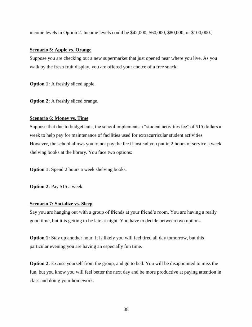
38

income levels in Option 2. Income levels could be $42,000, $60,000, $80,000, or $100,000.]

Scenario 5: Apple vs. Orange

Suppose you are checking out a new supermarket that just opened near where you live. As you

walk by the fresh fruit display, you are offered your choice of a free snack:

Option 1: A freshly sliced apple.

Option 2: A freshly sliced orange.

Scenario 6: Money vs. Time

Suppose that due to budget cuts, the school implements a “student activities fee” of $15 dollars a

week to help pay for maintenance of facilities used for extracurricular student activities.

However, the school allows you to not pay the fee if instead you put in 2 hours of service a week

shelving books at the library. You face two options:

Option 1: Spend 2 hours a week shelving books.

Option 2: Pay $15 a week.

Scenario 7: Socialize vs. Sleep

Say you are hanging out with a group of friends at your friend’s room. You are having a really

good time, but it is getting to be late at night. You have to decide between two options.

Option 1: Stay up another hour. It is likely you will feel tired all day tomorrow, but this

particular evening you are having an especially fun time.

Option 2: Excuse yourself from the group, and go to bed. You will be disappointed to miss the

fun, but you know you will feel better the next day and be more productive at paying attention in

class and doing your homework.

39

Scenario 8: Family vs. Money

Imagine that for the first time in three years, your parents (or if your parents are gone, your

closest relatives who are older than you) have arranged for a special family gathering that will

happen the day after Thanksgiving, with everyone also invited to Thanksgiving dinner. You face

two options. Would you choose to go to the family gathering the day after Thanksgiving (and

maybe to Thanksgiving dinner) if getting there required a $500 roundtrip plane ticket for plane

flights that were 5 hours each way?

Option 1: Go to the thanksgiving gathering, which requires a $500 round trip plane ticket.

Option 2: Miss the thanksgiving gathering, but save the money.

Scenario 9: Education vs. Social Life

Suppose you have decided to leave Cornell, and are transferring to a new school. You have been

accepted to two schools, and are deciding where to go. The first school is extremely selective and

high quality, but is in a small town out in the country with a less active social scene. The second

school is in a major city with a great social scene, but is slightly less renowned. Which would

you choose?

Option 1: Highly selective school, isolated socially and geographically.

Option 2: Less selective school, socially active and in a major city.

Scenario 10: Interest vs. Career

Suppose you are considering two summer internships. One is extremely interesting and involves

work you are passionate about, but does not advance your career. The other will likely be boring,

but will help you get a job in the future. Which would you choose?

Option 1: Interesting internship which does not advance career.

Option 2: Boring internship which will help you get a job.

40

Scenario 11: Concert vs. Duty

Say you are driving by yourself to see your favorite musician in concert on their last day in town.

You are five minutes away, and the concert starts in ten minutes. On the drive, you witness a

truck hit a parked car, causing roughly $500 in damages, and then drive away without leaving

their information. You notice the truck’s license plate, and you are the only witness. You face

two options:

Option 1: Keep driving and get to the concert on time.

Option 2: Call the police, in which case you will have to wait around the parked car to give a

testimony. This would take about half an hour. You would have trouble finding a seat and might

miss the whole concert.

Scenario 12: Low Rent vs. Short Commute

(Phrasing in Denver within-subject study): Say you are moving to a new town. You are trying to

decide between two similar apartments which you could rent. The two apartments are identical in

almost everything – including floor plan, amenities, neighborhood character, schools, safety, etc.

However, they have different rents and are located at different distances from your work.

Option 1: An apartment which requires a 45-minute drive to work. The rent is about 20% of

your monthly income.

Option 2: A similar apartment, with only a 10-minute drive. The rent is about 40% of your

monthly income.

(Version 2: Phrasing in Denver between-subject study): Say you are moving to a new town. The

new town is known for its terrible traffic jams, and driving there is widely considered to be

unpleasant. You are trying to decide between two similar apartments which you could rent. The

two apartments are identical in almost everything – including floor plan, amenities,

neighborhood character, schools, safety, etc. However, they have different rents and are located

41

at different distances from your work.

Option 1: An apartment which requires a 45-minute drive each way to work. The commute has

heavy traffic almost the whole way. The rent is about 20% of your monthly income.

Option 2: A similar apartment which requires a 10-minute drive each way to work. The

commute has heavy traffic almost the whole way. The rent is about 40% of your monthly

income.

Scenario 13: Friends vs Income

Say you have been reassigned at your job, and will be moved to a new location. There are two

offices where you could request to work. One office is in a city where many of your friends

happen to live, and pays 20% less than your current salary. The other office is in a city where

you don’t know anyone, and pays 10% more than your current salary. Your job will be exactly

the same at either office. You must decide between the following two options:

Option 1: Make 20% less than your current salary and move to the city with your friends.

Option 2: Make 10% more than your current salary and move to a city where you do not know

anyone.