what drives corporate asset prices: short- or long-run risk?

What Drives Corporate Asset Prices:

Short- or Long-Run Risk? ∗

Adelphe Ekponon†

Job Market Paper

September 13, 2017

This paper investigates the relative impact of various types of systematic risk on corporate asset

prices. Equity risk premium and credit spreads are priced in a consumption-based corporate finance

model with time-varying macroeconomic conditions. I decompose the risk premia into different

sources of systematic risk compensation and show that long-run risk commands most of the risk

premium (about 70%), for both equities and bonds. The role of long-run risk in the equity risk

premium is amplified in recessions, but remains stable over the business cycle for credit spreads.

The relative importance of short- vs. long-run risk also varies at the cross-section, thus providing

new testable implications.

JEL Codes: G12, G17, E44Keywords: Asset pricing, long-run risk, cross-section of returns, recursive preferences.

∗I am very grateful to my thesis supervisor Alexandre Jeanneret for constant support and many helpful discussions.I also thank Patrick Augustin, Frank Coggins, Christian Dorion, Jan Ericsson, Mathieu Fournier, Pascal Francois,Hyacinthe Some, Chao Xiong (discussant) and seminar participants at Universite de Sherbrooke, University ofToronto Ph.D Students in Finance Brownbag Seminar, and 2017 HEC-McGill Doctoral Workshop. Research supportsfrom HEC Montreal are gratefully acknowledged. All errors are mine.†HEC Montreal, Department of Finance, 3000 Cote-Sainte-Catherine, Montreal, Canada H3T 2A7. Phone:

(514) 473 2711. E-mail: [email protected]. Website: https://sites.google.com/site/adelpheekponon/

1 Introduction

The nature of risk premia is central for the understanding of asset prices. It is now widely accepted

that there exist different sources of systematic risk, which carry separate risk premium. First, firm

cash-flow shocks are partly systematic as they correlate positively with aggregate consumption.

Because these shocks are short-lived, the associated premium can be viewed as a compensation

for short-run risk. Second, the expected cash-flow growth rate is exposed to aggregate economic

conditions. That is, firms tend to grow less rapidly in recessions when expected consumption

growth is also low. Because expected growth rates are persistent, as they vary slowly over the

business cycle, the corresponding risk premium is a compensation for long-run risk. Consumption

based asset pricing models postulate that the first type of systematic risk is the main driver of

equity risk premium.1 More recent studies document that the second type helps explain some asset

pricing moments.2 It remains important, however, to understand the role of each type of risk for

the equity risk premium and corporate credit spreads.

This paper contributes to the literature in various dimensions. First, it decomposes and quan-

tifies the level of systematic risk and the associated risk premium. Second, it compares the role of

systematic risk across asset classes, equity versus debt. And third, it separates the risk premia into

the different sources of systematic risk to analyze their relative importance, both over the business

cycle and at the cross-section.

I propose a consumption-based asset pricing model that allows analyzing both types of sys-

tematic risk, individually or in tandem. The environment is characterized by time-varying macroe-

conomic conditions, which determine the expected growth rates of firm cash-flows and aggregate

consumption, as in Bansal and Yaron (2004), Bhamra, Kuehn, and Strebulaev (2010a; 2010b), and

Chen (2010). The representative agent is of an Epstein-Zin type. That is, this agent is not only

averse to short-run risk, but also has preference for early resolution of uncertainty, i.e. averse to

long-run risk.3 The approach to derive corporate asset prices follows the structural corporate finance

1See Rubinstein (1976), Lucas (1978), Breeden and Litzenberger (1978), and Breeden (1979).2Bansal and Yaron (2004) and Bhamra, Kuehn, and Strebulaev (2010b) show that time-varying expected growth

rates (and volatilities) generate high levels of the equity risk premium, while Bhamra, Kuehn, and Strebulaev (2010a)and Chen (2010) finds that such types of risk can explain the credit-spread puzzle.

3The coefficient of elasticity of intertemporal substitution (EIS) is greater than the inverse of the coefficient ofRRA.

1

models developed by Fischer, Heinkel and Zechner (1989), Leland (1994), and Hackbarth, Miao

and Morellec (2006).4 The firm’s optimal capital structure and default decisions are endogenously

determined.

The contribution is to separate the quantity from the price of risk, and to disentangle the

asset pricing implications of each source of systematic risk. I derive the credit spread in the full

model and isolate the quantity of risk component by assuming that the agent is risk neutral, i.e.

she does not command any risk premium. This is the pure compensation for holding default-

risky corporate bonds. The credit spread premium is defined by the difference between the total

credit spread and its default-risk compensation. Then, I separate the risk premia associated with

each type of systematic risk. The credit spread premium component that relates to short-run risk

is obtained by assuming that the agent has CRRA preferences.5 The long-run risk premium is

obtained by subtracting the short-run risk premium from the total credit spread premium. The

same methodology applies for the equity risk premium.

The model is calibrated to real consumption and aggregate firm profits data over the period

1952Q1–2015Q4. I respectively use U.S. real non-durables goods plus service consumption ex-

penditures and U.S. corporate profits before tax, both from the Bureau of Economic Analysis.

Short-run risk is determined by the correlation between consumption and corporate profits. Ag-

gregate economic conditions are considered to be time-varying and to switch between two states.

That is, the economy is either in expansion or in recession. The conditional expected growth rates

of consumption and firm cash-flows are computed using the NBER classification. The random

transition from one state to another is modeled by a two-states Markov-regime switching model,

following Hamilton (1989)’s approach. The transition matrix reveals that the states of the economy

tend to be persistent.

The main findings are as follow. First, systematic risk affects the expected excess return

differently for equities versus bonds. For corporate bonds, the quantity of risk represents around

63% of the total credit spread, while the corresponding risk premium captures 37%. This magnitude

is similar to what is observed empirically.6 In contrast, the compensation for systematic risk

4See also Goldstein, Ju, and Leland (2001) and Strebulaev (2007).5A CRRA agent has no preference for early resolution of the uncertainty, because the coefficient of elasticity of

intertemporal substitution is equal to the inverse of the coefficient of relative risk aversion.6Longstaff, Mithal, and Neis (2005) show that the default component represents 56% for A-rated bonds, 71% for

2

represents 100% of the equity risk premium, by definition.

Second, long-run risk commands a greater risk premium than short-run risk, when the agent has

a preference for early resolution of the uncertainty. This lends support to Bansal and Yaron (2004),

Tedongap (2014) and Bansal, Kiku, Shaliastovich, and Yaron (2014), who show that long-run

risk can help explain some stylized facts in asset pricing. I find that the long-run risk component

represents 72.8% of the total risk premium embedded into equity prices. The remaining 27.2%

represents a compensation for short-run risk, which arises when the investor is risk averse to cash-

flow shocks that positively correlate with aggregate consumption shocks. In contrast, the long-run

risk component of the credit spread premium represents 68.5%. These results show that the impact

of aversion to long-run risk, when the agent has recursive preferences, is significantly higher than

the aversion to short-run risk.

Third, the model shows how these risk premia vary over the business cycle. Long-run risk

represents 89.9% of equity risk premium in periods of economic downturns, but only 60.6% during

periods of economic expansion. Hence, the relative importance of long-run risk appears to be

strongly countercyclical for equity valuation. In contrast, the proportion of long-run risk in the

credit spread premium is stable over time, i.e. around 69%. Hence, stockholders price more their

preference for early resolution of the uncertainty during recessions than bondholders do.

Fourth, I find that the relative importance of these risk premia differs at the cross-section,

as it varies with firm characteristics. When idiosyncratic volatility increases, the proportion of

the credit spread premium due to long-run risk decreases. However, the model predicts that the

allocation of long-run vs. short-run risk in the equity risk premium is almost insensitive to the level

of indiosyncratic risk. When firms perform well and financial leverage decreases, the proportion of

the long-run risk premium decreases for equities but increases for bonds. These are novel testable

predictions. This paper also shows how preferences affect optimal debt and default decisions. When

the investor cares about long-run risk, the firm chooses to issue less debt and a lower default barrier.

This means that default probability is expected to be lower when corporate assets are valued by an

agent with recursive preferences. Hence, preferences affect the firms’ optimal decisions.

Finally, I consider an extension of the model in which cash-flow volatility varies over the business

BBB-rated bonds, and 83% for BB-rated bonds. Elton, Gruber, Agrawal, and Mann (2001) report that systematicrisk may explain up to 46% of the credit spread for 10-year corporates spread.

3

cycle. This creates a second source of long-run risk. I show that the conditional equity risk premium

is more countercyclical with time-varying cash-flow volatility, as reported in Bansal and Yaron

(2004). In presence of this additional source of risk, the proportion of the long-run risk component

in the equity risk premium decreases to 76.1% in recession (from 89.9% without time-varying

volatility) and increases to 67.6% in expansion (from 60.6% without time-varying volatility). In

contrast, the conditional credit spread premium increases in both states.

Overall, this paper helps us better understand the role of investor preferences and systematic

risk in corporate asset valuation. The results show that the compensation for long-run risk appears

to be the main component of the equity risk premium and corporate credit spreads. This paper

thus highlights the importance of the risk premium associated with an expected cash flow growth

rate that is time-varying and exposed to aggregate economic conditions. Yet the classical risk

premium associated with the consumption beta is not negligible, as it accounts for one third of the

total risk premium.

The remainder of the article is organized as follows. Section 2 reviews the literature. Section

3 describes the economy, details the sources of the systematic risks embedded into the model,

and the pricing of claims, Sections 4 and 5 present respectively the data and the methodology

proposed to measure the risk premiums, Section 6 studies the model’s implications, while Section

7 concludes. Proofs and others additional materials are contained in the Appendices.

2 Literature review

Asset pricing models like the capital asset pricing model (CAPM) of Markowitz (1952), Sharpe

(1964) and Lintner (1965) (and subsequent models as in Black, Jensen and Scholes (1972); Fama

and MacBeth (1973) have postulated that the sensitivity to market or systematic volatility is the

only risk that is needed to describe average returns.

However, since the 1970’s, several papers (see Basu (1977); Banz (1981); Shanken (1985);

Fama and French (1992; 1993)) proposed new approaches to improve the pricing performances

and provide answers to some of the inconsistencies of the CAPM, shown for example by empirical

analysis of cross-sectional asset data. In particular, the empirical asset pricing model proposed by

Fama and French (1992; 1993) is perhaps the most important. They demonstrate that CAPM has

4

virtually no explanatory power to explain the cross-section of average returns on assets of portfolios

sorted by size and book-to-market equity ratios, among others characteristics.

A second important trend of the literature has developed theoretical models to improve the

pricing performances of the CAPM via a consumption-based approach: the Consumption Capital

Asset Pricing Model (CCAPM). The main innovation of the CCAPM models lied on the introduction

of the macroeconomic risk into asset pricing. According to these first models, the risk premia

should be proportion to the consumption beta (correlation between the firm’s cash flow and the

consumption).

One line of this literature built on the market-based CAPM of Sharpe (1964) and Lintner

(1965), and on the Intertemporal CAPM developed by Merton (1973). The very first models

of CCAPM were issued by Rubinstein (1976), Lucas (1978), Breeden and Litzenberger (1978),

and Breeden (1979). However, the tests conducted on this line of the CCAPM models were not

concluding.7 Others authors have also argued that there exist some issues regarding the accuracy

of the consumption data due to the way they are recorded.8

Among the CCAPM models, another set of papers has introduced new features in the hope

to enhance the pricing performances.9 In particular, Epstein and Zin (1989) and Weil (1989)

have developed preferences, which allow for the separation between the intratemporal relative

risk aversion (CRRA) from the elasticity of intertemporal substitution (EIS). By introducing this

separability, it is now feasible to isolate, the aversion to future economic uncertainty from the

aversion to the current correlation between consumption and firm’s cash-flows. The later type of

aversion is measured through the consumption beta.

Alongside these papers, many empirical works have explored conditional versions of the con-

sumption CAPM as for example Jagannathan and Wang (2007) and Lettau and Ludvigson (2001a;

2001b).10 In particular, Lettau and Ludvigson (2001a; 2001b) explore a conditional version of

the consumption CAPM or CCAPM, by expressing the stochastic discount factor not in an un-

7See Hansen and Singleton (1983), Mehra and Prescott (1985), Chen, Roll, and Ross (1986) and, Hansen andJagannathan (1991).

8For example, Grossman, Melino, and Shiller (1987) and Breeden, Gibbons, and Litzenberger (1989)9See Pye (1972) and Greenig (1986) with time-multiplicative utility functions. See also Sundaresan (1989),

Constantinides (1990), Abel (1990), and Campbell and Cochrane (1999) with habit formation.10Predecessor works that have studies conditional versions of the CCAPM are Harvey (1991), Ferson and Harvey

(1991), Jagannathan and Wang (1996), and Ferson and Harvey (1999).

5

conditional linear model setting, as in traditional derivations of the CCAPM, but as a conditional

factor model. Empirically, their model performs as good as the Fama-French three-factor model

in explaining the cross-section of average returns of portfolios sorted by size and book-to-market

value. Lettau and Ludvigson’s conditional model captures the countercyclical risk premium and

improves the performance of the CCAPM. The reason is that the correlation between stocks and

the consumption growth increases more in bad times, when risk aversion is high, compare to the

good times when the risk aversion is low. According to their findings, this conditionality on risk

premia is missed by unconditional CCAPM models because they produce constant risk premia over

time.

This indicates that the most suitable assets pricing models should incorporate not only investors

preferences but also conditional pricing. Bansal and Yaron (2004)and recent papers by Bhamra,

Kuehn, and Strebulaev (2010a; 2010b) and Chen (2010), have successfully developed consumption-

based models with a representative agent with Epstein-Zin-Weil type of preference and in a time-

varying macroeconomic environment. This type of agent is not only risk-averse but also dislikes

the uncertainty about the future macroeconomic conditions. These papers achieve the objective to

disentangle the impact of these two types of preferences on equity and debt and show that these

preferences help resolve the credit spread puzzle and to generate reasonable levels of equity risk

premium. However, this paper emphasizes on how much pure long-run risk actually influences risk

premia.

3 The model setup

The economy consists of a representative agent and several firms. The agent provides capital to

the firm by buying equity and bond. There is no friction in the economy.

3.1 Firm cash-flows

Let assume the representation firm has a stream of cash-flows, denoted by Xt, which is given by

the stochastic process:

6

dXt

Xt

= µstdt+ σiddBidt + σgdBt, st = {R,E} . (1)

First, cash-flows are affected by continuous systematic shocks, dBt. Second, the expected growth

rate varies with global conditions. In this economy, there are two different economic conditions

- expansion, E and, recession, R. The state of the economy, st, switches from one economic

condition to another randomly. The switching is modeled through a two-states Markov process.

This random change in the state of the economy happens infrequently. Therefore, each state

tends to be persistent. The firm state-dependent cash-flows growth rate, µst , is procyclical so that

µE > µR . Cash-flows also experience idiosyncratic shocks, dBidt , so that, the total volatility of

cash-flows equals to σX =√

(σid)2 + (σg)2. The standard Brownian motions measure Bidt and Bt

are independent.

3.2 Representative agent

3.2.1 Consumption

The representative agent prices firm claims. Her consumption has an exogenous stream Ct. Let

assume Ct follows the stochastic process:

dCtCt

= θstdt+ σdBC,t, st = {R,E} , (2)

where, the state-dependent consumption growth rate, θst , is procyclical so that θE > θR and σ

is the consumption volatility. The standard Brownian motion under the physical measure BC,t

represents the continuous shocks to the consumption. Because firm cash-flows correlate with these

shocks, the processes BC,t and Bt are correlated.

3.2.2 Stochastic discount factor

The representative agent has Epstein-Zin-Weil preference.11 This preference separates the impacts

of risk aversion, γ from the elasticity of intertemporal substitution, defined by the EIS coefficient,

11This type of utility function, developed by Kreps and Porteus (1978), Epstein and Zin (1989), Duffie andEpstein (1992), and Weil (1989).

7

ψ. In equilibrium, the state-price density dynamic follows:

dπtπt

= −rstdt+dMt

Mt

(3)

= −rstdt−ΘBdBt + ΘPstdNst,t, (4)

where Mt is a martingale under the physical measure, Nst,t a Poisson process which jumps

upward by one whenever the state of the economy switches from the state st to the state st 6= st,

ΘB = γσ is the market price of risk due to Brownian shocks in the state st, ΘPst = ∆st − 1 is the

market price of risk due to random changes of the state of economy from st = {R,E}, where ∆st ,

is the change in the state-price density πt at the transition time from state st = {R,E}.

3.2.3 Price of short-run risk

Firms cash-flows are affected by macroeconomic shocks, that also affects consumption. Call, ρ, the

coefficient of correlation between cash-flows and consumption. The agent cannot diversify away

those shocks that positively correlate with her consumption. This will lead the agent to ask a price

for this risk above the compensation that a risk neutral agent should demand. This additional

compensation is obtained by viewing the firm’s cash flows as more risky than in reality. In this

regard, the agent derives a risk-neutral measure of cash flows growth rate, µst , by reducing the

physical rate so that µst = µst−γρσgσ, where γ is the constant coefficient of relative risk aversion

which is independent from the EIS. The agent has risk aversion if γ > 0 and is risk neutral if γ = 0.

3.2.4 Price of long-run risk

The time-varying consumption and cash flows growth rates incorporates the long-run risk into the

model. More precisely, these consumption and cash flows moments depend on the state of the

economy. Consequently, in presence of the long-run risk, the agent prices assets as if recessions

last longer than in reality and so expansion last shorter than in reality. This preference originates

from the fact that the agent does not like not knowing when next recession will arrive since this

state of the economy corresponds to weaker cash-flows growth rates at the time when consumption

growth is also low.

8

Call, λst , the probability per unit of time of leaving state st. Hence, the quantity 1/λst is the expected

duration of state st. However, recessions are shorter than expansions, so that 1/λR < 1/λE. Thus,

the physical probabilities λR and λE are converted to their risk-neutral counterparts λR and λE

through the factor ∆E, which is the change in the state-price density πt at the transition time from

expansion to recession. The risk-neutral probabilities per unit of time of changing state are then

given by

λE = ∆EλE and λR = ∆RλR =1

∆E

λR. (5)

When ψ > 1γ

, the agent has preference for earlier resolution of the uncertainty, i.e. ∆E > 1. In

contrast, the agent is indifferent to earlier resolution of the uncertainty about the future states of

the economy if ∆E = ∆R = 1, i.e. when ψ = 1γ

. This is a CRRA agent who would use the actual

probability to price assets, i.e. λE = λE and λR = λR.

3.3 Asset prices

Equity and debt are issued at initial time s0 = {R,E}, thus their values depend on the financing

states as well as on the current st = {R,E}.

3.3.1 Bond price

The present debt value, Bst , is the discounted coupon stream c before default plus the present value

of the recovered firm asset liquidation value at default (φsDAsD), where φst is the state-dependent

asset recovery rate and Ast is the firm asset liquidation value. Hence,

Bst = Et

[∫ tD

t

cπuπtdu | st

]+ Et

[πuπtφtDAtDdu | st

]. (6)

The credit spread, CSst , for the present state st = {R,E} is defined by

CSst =c∗

Bst

− rB,st (7)

9

where c∗ is the optimal coupon value and rB,st is the perpetual risk-free discount.

3.3.2 Stock price

The stock value, Sst , is the after-tax discounted value of future cash-flows, Xt less coupon pay-

ments, c before bankruptcy is declared by the stockholders.

Sst = (1− τ)Et

[∫ tD

t

πuπt

(Xt − c) du | st]

(8)

where tD is the random default time. The absolute priority rule holds so that at default equity

value is worthless.

The levered equity risk premium, RPst , for the current state st = {R,E} is

RPst = γρσBstσ + (1−4st)σPstλst (9)

with σBst = XtSst

∂Sst∂Xt

σg is the systematic volatility of stock returns caused by Brownian shocks,

where Sst represents the equity value and σPst =SjSi− 1, i 6= j = {R,E} the volatility of stock

returns caused by the change of state of the economy. The first term (γρσBstσ) corresponds to the

compensation asked by investors to bear the short-run risk and the second term, (1−4st)σPstλst ,

to the price associated to the long-run risk, where ∆st , is the change in the state-price density πt

at the transition time from state st = {R,E}.

3.4 Firm decisions

The coupon value is chosen by shareholders at the time debt is issued to maximize the firm value

cs0 = argmax(Ds0 + Ss0), where s0 = {R,E} is the financing state. The shareholders also

determine the ex-ante default boundaries, XD,st , corresponding to each state of the economy with

the objective to optimize the equity value, so that:

10

∂Sst∂Xt

|Xt=XD,st = 0 (10)

4 Data and model calibration

This section presents the calibration of the model. Table 1 summarizes the parameter values. The

model is calibrated to match the salient aspects of the market.

Table 1 [about here]

NBER dates are used to characterize the U.S. business cycle. The state of the economy can

be either expansion (E) or recession (R). The switch from one state to another, which occurs

randomly, is modeled by a Markov chain. The actual probability of transition from one state to

another, λst , the actual long-run probability of being in each state, fst , and the actual rate of

news arrival, denoted by p, are estimated using a two-state Markov-regime switching model on

NBER recession dates over the period 1952Q1-2015Q4.12 The estimation approach is based on

Hamilton (1989) and detailed in Appendix F. Real non-durables goods plus service consumption

expenditures obtain from the Bureau of Economic Analysis is used as proxy of the aggregate

consumption. The estimates of the actual probabilities of being in a expansion and in recession

are respectively fE = 85.16% and fR = 14.84%. When calibrating the conditional moments of

consumption growth to the NBER recession dates, I obtain a U.S. consumption growth rate of

θL = 0.65% in recession and θE = 2.20% in expansion, while its unconditional systematic volatility

is σ = 0.86%.

The cash-flows data are the quarterly corporate profits (without inventory valuation and capital

consumption adjustment) in billions of dollar before tax from the US Bureau of Economic Analysis.

I use information over the period 1952Q1-2015Q4 to compute the moments of the representative

12Following Boguth and Kuehn (2013) and Lettau, Ludvigson, and Wachter (2008), I use postwar data. Romer(1989) has shown that data on consumption recorded at the prewar period are not reliable since they containsignificant measurement errors.

11

firm cash-flows growth.13 The conditional growth rate is thus equal to µR = −13.47% in recession

and µE = 5.62% in expansion while its unconditional standard deviation σg = 11.82%. The debt

recovery rate is set to αR = 40% in recession and αE = 70% in expansion. Chen (2010) estimates

that mean bond recovery rate is 41.8%. Longstaff, Mithal, and Neis (2005) use a recovery rate of

50% and Duffee (1999), 44% using Moody’s data. The corporate tax rate τ is set at 15%.

Regarding the representative agent’s preferences, I consider a coefficient of risk aversion γ = 10,

a coefficient of elasticity intertemporal substitution (EIS) ψ = 1.5, and an annual discount rate

equal to β = 3.0%.

With this calibration, the default probability is very high in recession (around 12%), whereas

this probability is less than 1% in expansion. The equity risk premium is 0.88% in expansion and

3.56% in recession, showing that the equity risk premium is countercyclical. Interestingly, the

unconditional credit spread obtained by computing fR×CSfullR + fE×CSfullE , is equal to 117 bps

and the unconditional equity risk premium, obtained by computing fR ×RP fullR + fE ×RP full

E , is

equal to 1.282%. This is consistent with the admitted observation that the risk levels embedded

into stocks should not be significantly higher than those carried by bonds. This unconditional

equity risk premium computed by assuming rational expectation, is consistent with what similar

models will predict. Bhamra, Kuehn, and Strebulaev (2010a; 2010b) and Chen (2010) simulate

an economy consisting of a cross-section of firms which helps increase significantly the equity risk

premium, with the objective to resolve the equity premium puzzle. However, this paper addresses

the question of the relative impact of the short-run risk, as in CAPM model, versus the long-run

risk, as in models that incorporate macroeconomic risk. Here, I focus on modeling an individual

firm which is sufficient to achieve this goal.

5 Methodology to measure the risk premia

This section describes the procedure that I follow to separately retrieve the long- and short-run risk

components of risk premia. For bond pricing, the actual compensation demanded by investors is

the sum of the default risk component and risk premia. Hence, the default risk component is the

remaining part of the credit spread after the risk premia component is removed.

13The earnings data start in 1952 to match the consumption data.

12

5.1 Measuring the short-run risk premium

If investors have no aversion to the short-run risk, this means that they use the physical cash-flow

growth rate µst , instead of the risk neutral one µst to price corporate claims. In this case, the

investors are neutral regarding the fact that corporate cash-flows are correlated to their consump-

tion. Hence, I measure the short-run risk premium by comparing the full model with a model that

sets µst = µst . For corporate bonds, the short-run risk premium is CSSRst = CSfullst − CSµst=µstst .

For equity, the short-run risk premium is RP SRst = RP full

st − RP µst=µstst . Analytically, the equity

risk premium due to short-run risk equals to γρσBσ as shown in the section 3.3.2.

5.2 Measuring the long-run risk premium

Similarly, if investors do not care about long-run risk they use the physical probability of being in

state st, fst instead of the risk neutral one fst to price firm assets. Hence, I measure the long-run

risk premium by comparing the full model with a model that sets fst = fst . For corporate bonds,

the long-run risk premium equals to CSLRst = CSfullst − CSfst=fstst . For equity, the long-run risk

premium yields RPLRst = RP full

st −RPfst=fstst . Analytically, the equity risk premium related to the

preference for early resolution of the uncertainty equals to (1 −4ss)σPssλst , where λst = pfst as

shown in the section 3.3.2.

5.3 Measuring the compensation for default risk

The default risk component is obtained by assuming that investors have CRRA preferences. That

is, they use physical measure of cash-flow growth rate µst and actual probability of being in state st,

fst . Alternatively, this compensation, embedded into the credit spread, is measured by subtracting

premia due to long- and short-run risks from the full model predictions. Hence, for corporate

bonds, the default risk component equals to CSQst = CSfullst −CSLRst −CS

SRst . For the equity risk

premium, the compensation for default risk is worthless, i.e. RPQst = RP full

st −RPLRst −RP

SRst = 0.

13

6 Theoretical predictions

This part presents and discusses the theoretical predictions of the paper. The main objective are to

disentangle, first, the impacts of investor preferences from default risk component into corporate

asset prices, then, compare the relative proportions of the long- and short-run risk premia. Without

loss of generality, it is assumed that firms finance themselves in expansion. Predictions are done

for the same economy but assuming various types of agent. In the last section, I compare different

economies in which the firm can account for investor preferences while choosing its optimal policies.

6.1 Quantity vs price of risk

This section presents the findings concerning the quantity and price of risk embedded into the

equity risk premium and credit spread. The predictions are done for the full model which I compare

with the three following special cases: i) when the agent does not about long-run risk, ii) when the

investor has no aversion to the short-run risk and, finally iii) when the investor is risk-neutral. The

economy is the same for all cases, i.e. coupon and barriers are kept constant to those of the full

model for all cases. I used the methodology explained in the section 5 to produce the risk premia

due to the two systematic risks (short- and long-run risks) and, then, the quantity of risk, which

is also obtained from the case iii) predictions. The table 2 reports the main results for the four

cases (full model, case i, case ii and case iii) and the table 3 reports the quantity of risk and the

risk premiums related to each type of systematic risk as well as their weights into both the total

equity risk premium and credit spread.

Tables 2 and 3 [about here]

The proportion of the default risk, into the credit spread, is about 63% (or 74.34 bps), the

remaining representing the credit spread premium (42.7 bps). In a risk-neutral setting, Chen,

Collin-Dufresne, and Goldstein (2009) find an average four-year Baa credit spreads of 86.8 bps

and 5.6 bps for Aaa. This proportion of default risk in bond spread (i.e. 63%) stays constant

across the states of the economy. Similar structural models are designed to capture the average

14

spread of A-rated and B-rated bonds.14 This finding also matches those of Longstaff, Mithal, and

Neis (2005), who have estimated that the default component accounts for 51% of the spread for

AAA-rated and 71% for BBB-rated bonds.

Since it is a premium for holding stocks, the equity risk premium carries no quantity of risk.

Indeed, for a risk-neutral agent to both short-run (γ = 0) and the long-run (∆E = ∆R = 1) risks,

the equity risk premium yields zero, as it can be seen with the equation 9. The figure 1 summarizes

these findings.

Figure 1 [about here]

The remaining sections focus on the risk prices embedded into corporate assets.

6.2 Importance of the preference for earlier resolution of the uncertainty

The unconditional price of long-run risk represents 72.8% of the equity risk premium. Hence, a

little than one-fourth of the equity risk premium originates from the correlation between firm cash

flows and consumption. 68.5% of the credit risk premium comes from investors’ willingness to

see a quick resolution of the uncertainty regarding the subsequent states of the economy and the

remaining is due to the short-run risk. This confirms the macroeconomic risk as the main source

of uncertainty in the pricing of corporate assets and this is particularly true in an economy in which

the investor prefers quicker resolution of uncertainties regarding the future conditions.

However, many reasons may explain the weak impact of the risk aversion on corporate assets

prices compared to the aversion to macroeconomic risk.

For equity pricing, this stylized fact has been extensively reported 15. Chen, Roll, and Ross

(1986) performed an empirical test of classical consumption-based models, which postulate that

the main factor in asset pricing should be the covariance with the aggregate consumption as in the

classical CCAPM models like Rubinstein (1976) or Lucas (1978). They found that this factor is

14Bhamra, Kuehn, and Strebulaev (2010a; 2010b) restrict their analysis, as in many other papers, to BBB-rateddebt. As they pointed out the spreads of top graded bonds (AAA or AA-rated) are mostly dominated by factorsother than credit risk, and that structural models work well for low-grade bonds (B-rated and below). Similarly,Chen (2010) also focus mainly on Baa-rated firms (Baa in Moody’s being equivalent to BBB in the S&P notationsystem).

15See Hansen and Singleton (1983), Mehra and Prescott (1985) and, Hansen and Jagannathan (1991).

15

not sufficient to explain stock prices. This also provides evidence for the Fama and French (1993)

findings that the correlation with the market alone cannot explain stocks prices. Bansal and Yaron

(2004) provide empirical support for a model with aggregate consumption and dividend processes

that contain a small persistent expected growth rate component and a conditional volatility com-

ponent, in conjunction with Epstein-Zin-Weil preferences to explain many asset pricing puzzles.

This underpins further the preeminent role of long-run risk in driving corporate assets prices. Here,

the poor impact of the short-run risk, on equity value, can easily be measured. The associated

equity premium is measured by γρσBstσ, with σBst = XtSst

∂Sst∂Xt

σg =∂lnSst∂lnXst

σg the systematic volatility

of stock returns induced by Brownian shocks. However, the U.S. consumption growth volatility

σ is around 1% (see Table 1) in the data, the corporate earnings growth volatility σg is around

12% and, the correlation between earnings and the consumption ρ is about 25%. Because of the

fact that the term∂lnSst∂lnXst

(which is the responsiveness of stock price to a change in cash-flow)

is bounded, γρσBstσ will stay relatively small. Consequently, the short-run risk will have a limited

impact on stocks. A recent work by Bali and Zhou (2016) proposes a conditional intertemporal

capital asset pricing model with time-varying market risk and economic uncertainty. As in the

approach developed in this paper, the risk price on equity is composed of two separate terms; the

first term compensates for the standard market risk and the second term represents additional pre-

mium for economic uncertainty. They back up their model with empirical analysis to test whether

the time-varying conditional covariances of equity returns with the market or economic uncertainty

predicts the time-series and cross-sectional variation in stock returns. This study also concludes

that exposures to economic uncertainty better predict stock returns. This finding is also supported

by Lettau, Ludvigson, and Wachter (2008) who document that the fall in macroeconomic risk has

lead to exceptional high aggregate stock prices in the 1990 and that this phenomenon persists

today.

Regarding the bond pricing, using credit default swap (CDS) spreads, Tang and Yan (2010)

document that average credit spreads are decreasing in GDP growth rate, but increasing in GDP

growth volatility and that, credit spreads are lower for smaller systematic jump risk. These results

support the role of macroeconomic uncertainties in corporate bonds value as well.

As pointed out in Fama and French (1993), common factors seem to drive the returns on stocks

16

and bonds. They document that stock and bond returns are related through shared variation in the

bond-market factors. Besides low-grade corporates, the bond-market factors, namely maturity and

default risk (but not directly the market risk) capture the common variation in bond returns. Most

importantly, they have identified five factors including the market risk that may explain average

returns on both stocks and bonds. The implications of these results are twofold. First, the aversion

due to the correlation between consumption and cash-flows (a proxy for the market risk) does not

have significant repercussions on credit risk spread premium. Second, others common factors,

which at least some of them are likely to vary with macroeconomic conditions, capture more of

risk premia than market risk alone.

This paper provides support to these results and gives a better understanding as to why the

long-run risk is dominant.

6.3 Countercyclical risk premia

The equity risk premium is 3.59% in bad times and 0.88% in good times. In particular, the

compensation asked by investors to bear the risk associated with the uncertainty about future

economic conditions represents 89.9% of the equity risk premium or an annual required rate of

return of 3.23%, in bad times, while it worths 60.62% in recession or 0.53%.

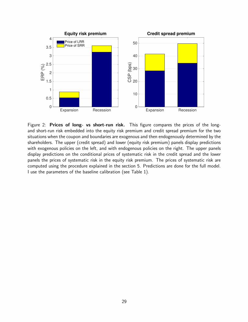
On average, the credit spread premium is 49.7 bps in bad times and 41.5 bps in good times.

However, Regardless of the state of the economy, the proportion of the credit spread premium due

to the long-run risk represents 70% of the total price of risk while the remaining 30% comes from

the sensitivity of the firm cash-flow to the consumption.

Lettau and Ludvigson (2001a; 2001b)16 explore a conditional version of the consumption CAPM

and found that their model performs as good as the Fama-French three-factor model in explaining

the cross-section of average returns of portfolios sorted by size and book-to-market value. They

document that countercyclical risk premium help improve assets pricing.

16Bekaert, Engstrom, and Xing (2009), Bansal, Kiku, Shaliastovich, and Yaron (2014) and Bali and Zhou (2016)also provide support for time-varying risk prices.

17

6.4 Investors’ preferences

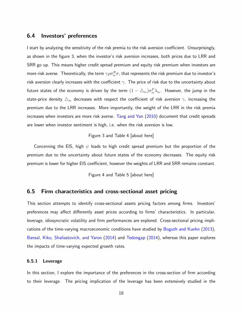
I start by analyzing the sensitivity of the risk premia to the risk aversion coefficient. Unsurprisingly,

as shown in the figure 3, when the investor’s risk aversion increases, both prices due to LRR and

SRR go up. This means higher credit spread premium and equity risk premium when investors are

more risk averse. Theoretically, the term γρσBstσ, that represents the risk premium due to investor’s

risk aversion clearly increases with the coefficient γ. The price of risk due to the uncertainty about

future states of the economy is driven by the term (1 − 4st)σPstλst . However, the jump in the

state-price density 4st decreases with respect the coefficient of risk aversion γ, increasing the

premium due to the LRR increases. More importantly, the weight of the LRR in the risk premia

increases when investors are more risk averse. Tang and Yan (2010) document that credit spreads

are lower when investor sentiment is high, i.e. when the risk aversion is low.

Figure 3 and Table 4 [about here]

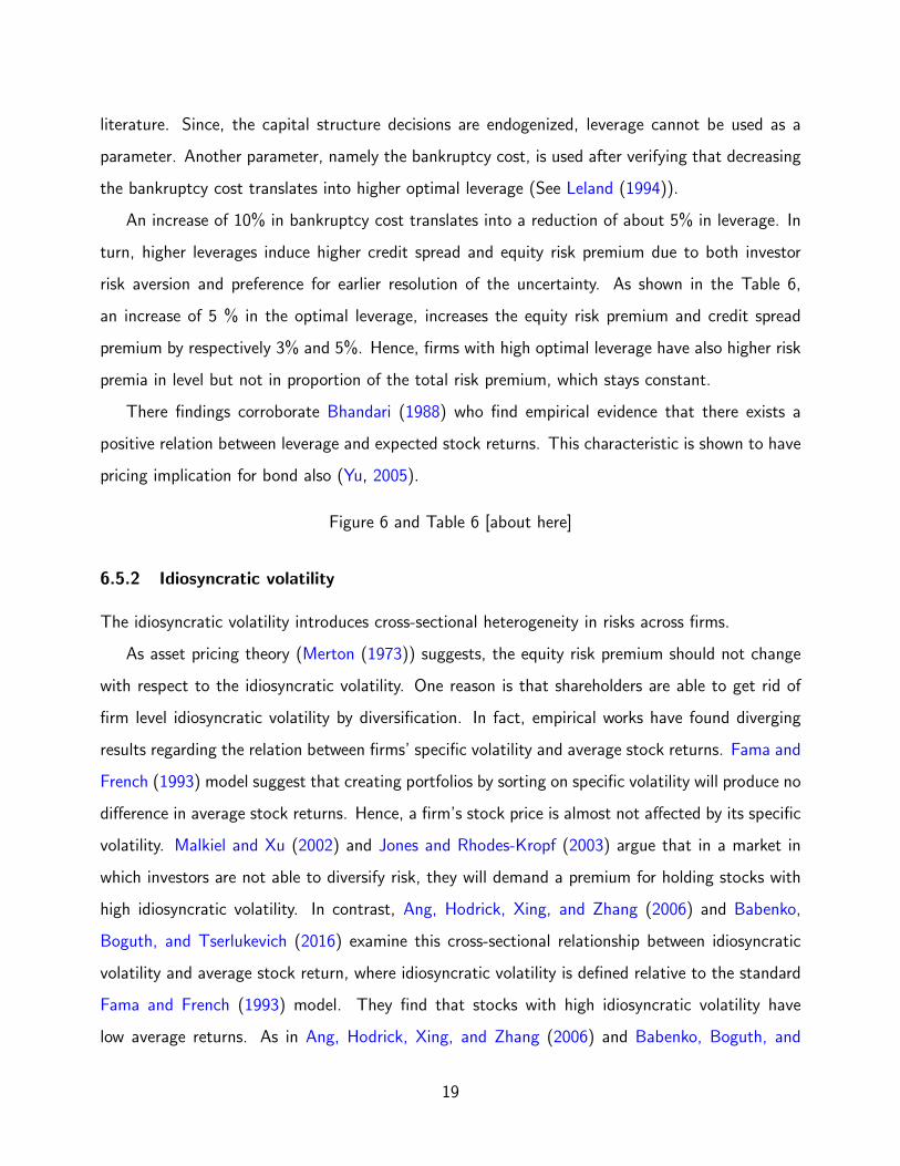
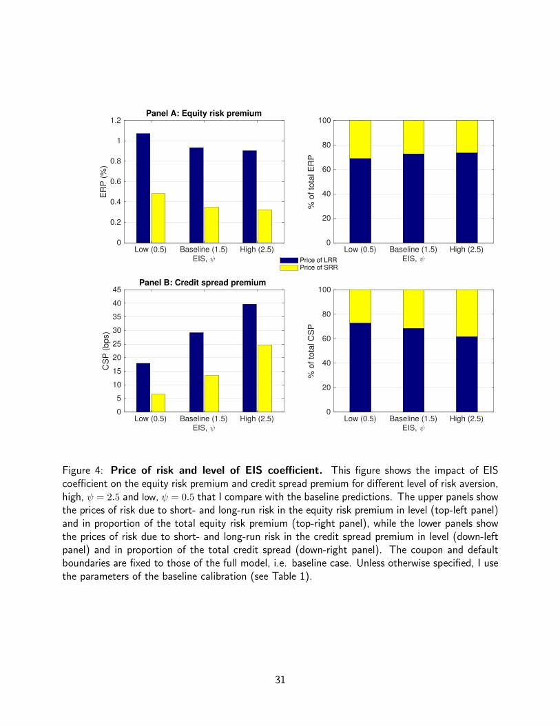
Concerning the EIS, high ψ leads to high credit spread premium but the proportion of the

premium due to the uncertainty about future states of the economy decreases. The equity risk

premium is lower for higher EIS coefficient, however the weights of LRR and SRR remains constant.


6.5 Firm characteristics and cross-sectional asset pricing

This section attempts to identify cross-sectional assets pricing factors among firms. Investors’

preferences may affect differently asset prices according to firms’ characteristics. In particular,

leverage, idiosyncratic volatility and firm performances are explored. Cross-sectional pricing impli-

cations of the time-varying macroeconomic conditions have studied by Boguth and Kuehn (2013),

Bansal, Kiku, Shaliastovich, and Yaron (2014) and Tedongap (2014), whereas this paper explores

the impacts of time-varying expected growth rates.

6.5.1 Leverage

In this section, I explore the importance of the preferences in the cross-section of firm according

to their leverage. The pricing implication of the leverage has been extensively studied in the

18

literature. Since, the capital structure decisions are endogenized, leverage cannot be used as a

parameter. Another parameter, namely the bankruptcy cost, is used after verifying that decreasing

the bankruptcy cost translates into higher optimal leverage (See Leland (1994)).

An increase of 10% in bankruptcy cost translates into a reduction of about 5% in leverage. In

turn, higher leverages induce higher credit spread and equity risk premium due to both investor

risk aversion and preference for earlier resolution of the uncertainty. As shown in the Table 6,

an increase of 5 % in the optimal leverage, increases the equity risk premium and credit spread

premium by respectively 3% and 5%. Hence, firms with high optimal leverage have also higher risk

premia in level but not in proportion of the total risk premium, which stays constant.

There findings corroborate Bhandari (1988) who find empirical evidence that there exists a

positive relation between leverage and expected stock returns. This characteristic is shown to have

pricing implication for bond also (Yu, 2005).


6.5.2 Idiosyncratic volatility

The idiosyncratic volatility introduces cross-sectional heterogeneity in risks across firms.

As asset pricing theory (Merton (1973)) suggests, the equity risk premium should not change

with respect to the idiosyncratic volatility. One reason is that shareholders are able to get rid of

firm level idiosyncratic volatility by diversification. In fact, empirical works have found diverging

results regarding the relation between firms’ specific volatility and average stock returns. Fama and

French (1993) model suggest that creating portfolios by sorting on specific volatility will produce no

difference in average stock returns. Hence, a firm’s stock price is almost not affected by its specific

volatility. Malkiel and Xu (2002) and Jones and Rhodes-Kropf (2003) argue that in a market in

which investors are not able to diversify risk, they will demand a premium for holding stocks with

high idiosyncratic volatility. In contrast, Ang, Hodrick, Xing, and Zhang (2006) and Babenko,

Boguth, and Tserlukevich (2016) examine this cross-sectional relationship between idiosyncratic

volatility and average stock return, where idiosyncratic volatility is defined relative to the standard

Fama and French (1993) model. They find that stocks with high idiosyncratic volatility have

low average returns. As in Ang, Hodrick, Xing, and Zhang (2006) and Babenko, Boguth, and

19

Tserlukevich (2016), this paper’s approach provides a negative relationship between idiosyncratic

volatility and equity risk premium (see upper panels of Figure 7). This is the case for both the

short-run and long-run risks. This paper further predicts that the weights of LRR and SRR in

equity premium do not change with idiosyncratic volatility.

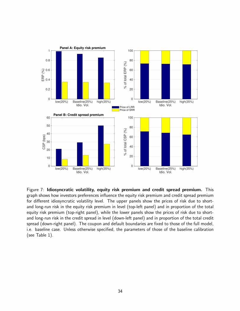
Regarding bond valuation, the level of the price of risk embedded into the credit spread increases

with firm specific volatility. Moreover, even if the impact of LRR is higher, SRR’s impact also

increases as the firm specific volatility goes up. An increase in volatility from 25% to 35% leads

to a nearly 80 % increase of the credit spread premium, i.e. from 42.7 to 77.5 bps. In term of

proportion, the impact of the LRR is reduced for firms with high level of idiosyncratic volatility. In

the cross-section, Tang and Yan (2010) found out that firm-level cash-flow volatility raises credit

spreads. Exploring the quality of a firm’s information disclosure on the term structure of its bond

yield spreads, Yu (2005) documents that firms with high volatility behave differently compared to

firms with low volatility.


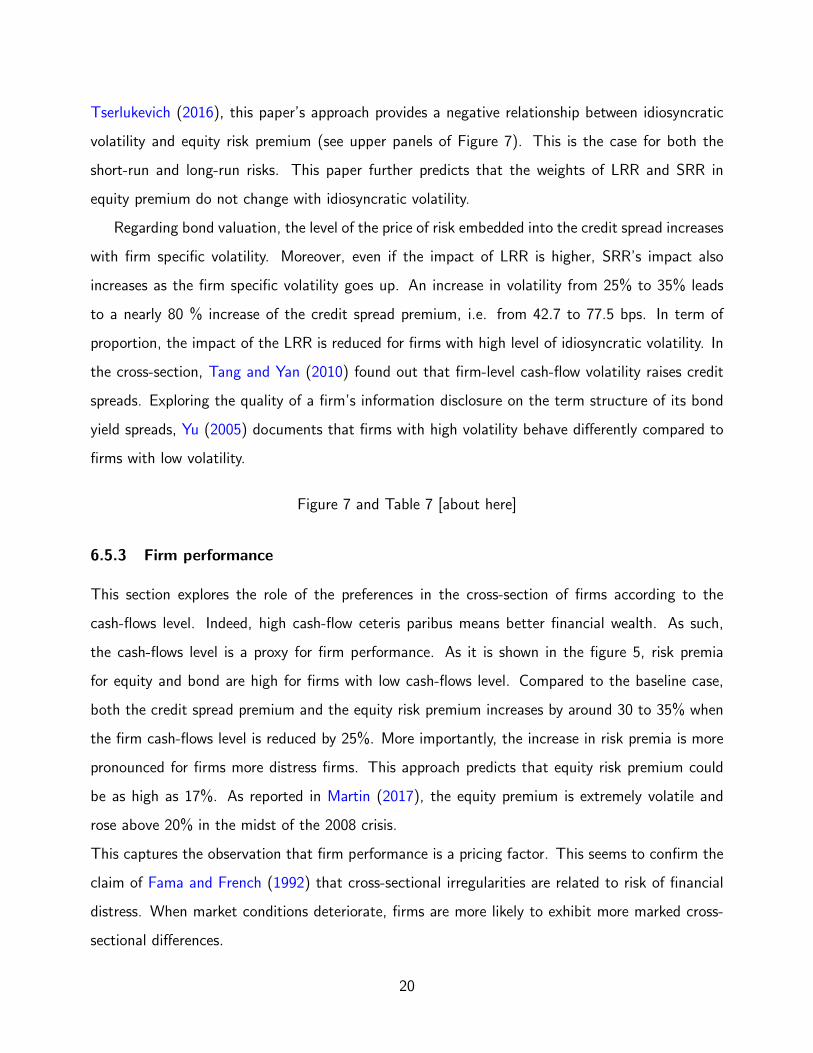
6.5.3 Firm performance

This section explores the role of the preferences in the cross-section of firms according to the

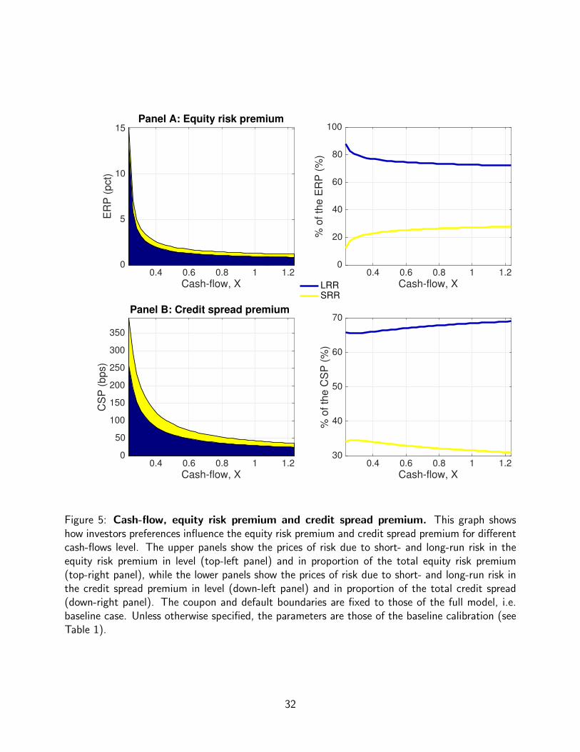
cash-flows level. Indeed, high cash-flow ceteris paribus means better financial wealth. As such,

the cash-flows level is a proxy for firm performance. As it is shown in the figure 5, risk premia

for equity and bond are high for firms with low cash-flows level. Compared to the baseline case,

both the credit spread premium and the equity risk premium increases by around 30 to 35% when

the firm cash-flows level is reduced by 25%. More importantly, the increase in risk premia is more

pronounced for firms more distress firms. This approach predicts that equity risk premium could

be as high as 17%. As reported in Martin (2017), the equity premium is extremely volatile and

rose above 20% in the midst of the 2008 crisis.

This captures the observation that firm performance is a pricing factor. This seems to confirm the

claim of Fama and French (1992) that cross-sectional irregularities are related to risk of financial

distress. When market conditions deteriorate, firms are more likely to exhibit more marked cross-

sectional differences.

20

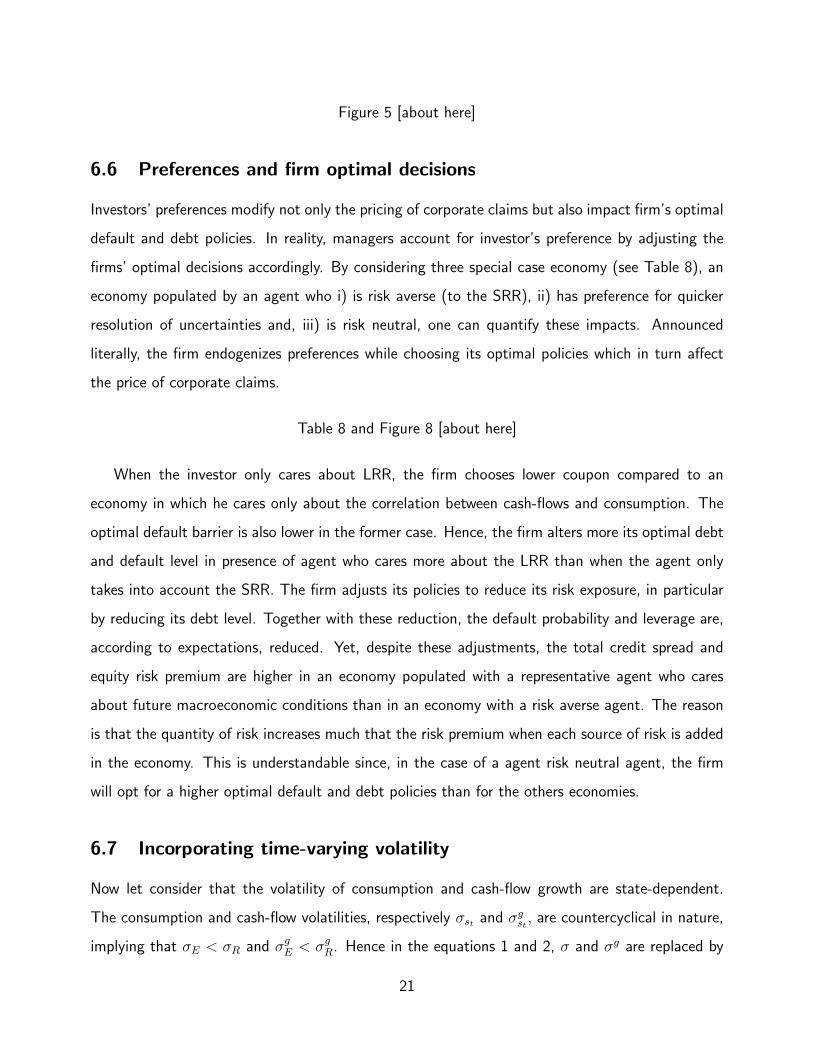
Figure 5 [about here]

6.6 Preferences and firm optimal decisions

Investors’ preferences modify not only the pricing of corporate claims but also impact firm’s optimal

default and debt policies. In reality, managers account for investor’s preference by adjusting the

firms’ optimal decisions accordingly. By considering three special case economy (see Table 8), an

economy populated by an agent who i) is risk averse (to the SRR), ii) has preference for quicker

resolution of uncertainties and, iii) is risk neutral, one can quantify these impacts. Announced

literally, the firm endogenizes preferences while choosing its optimal policies which in turn affect

the price of corporate claims.

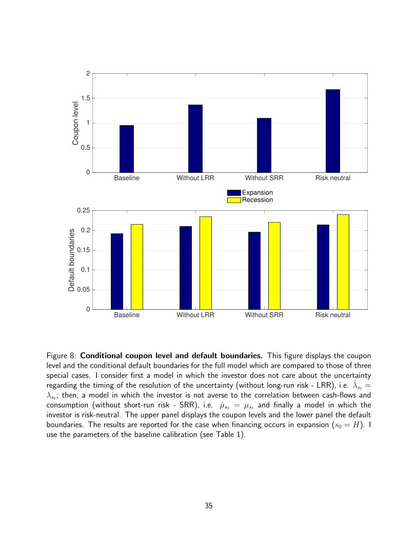
Table 8 and Figure 8 [about here]

When the investor only cares about LRR, the firm chooses lower coupon compared to an

economy in which he cares only about the correlation between cash-flows and consumption. The

optimal default barrier is also lower in the former case. Hence, the firm alters more its optimal debt

and default level in presence of agent who cares more about the LRR than when the agent only

takes into account the SRR. The firm adjusts its policies to reduce its risk exposure, in particular

by reducing its debt level. Together with these reduction, the default probability and leverage are,

according to expectations, reduced. Yet, despite these adjustments, the total credit spread and

equity risk premium are higher in an economy populated with a representative agent who cares

about future macroeconomic conditions than in an economy with a risk averse agent. The reason

is that the quantity of risk increases much that the risk premium when each source of risk is added

in the economy. This is understandable since, in the case of a agent risk neutral agent, the firm

will opt for a higher optimal default and debt policies than for the others economies.

6.7 Incorporating time-varying volatility

Now let consider that the volatility of consumption and cash-flow growth are state-dependent.

The consumption and cash-flow volatilities, respectively σst and σgst , are countercyclical in nature,

implying that σE < σR and σgE < σgR. Hence in the equations 1 and 2, σ and σg are replaced by

21

σst and σgst , where σR = 1.23% in recession and σE = 0.80% in expansion and σgR = 24.61% in

recession and σgE = 9.59% in expansion.

Equity risk premium is more countercyclical with time-varying volatility of consumption and

cash-flow, as reported in Bansal and Yaron (2004). This feature introduces more (less) risk in

recessions (expansion). With time-varying volatility, the conditional total price of risk in equity risk

premium is 4.45% in recession as opposed to 3.56% without and 0.80% in expansions as compared

to 0.88% without. However, because of the countercyclicality of volatility, the proportion of the

LRR becomes only 76.6% (instead of 89.9% without time-varying volatility) and 67.6% (instead

of 60.6% without time-varying volatility).

Credit spread premium increases in both states, respectively from 49.64 to 58.46 bps in re-

cessions and from 41.51 to 47.21 bps in expansion when adding time-varying volatility to the

model.

Table 9, Table 10 and Table 11 [about here]

This approach allows to retrieve separately from discount rate news, risk premia due to con-

sumption volatility news as in Boguth and Kuehn (2013) and Bansal, Kiku, Shaliastovich, and

Yaron (2014).

7 Concluding remarks

Investor’s preferences influence firm decisions, hence affecting the valuation of the firm’s claims.

Thus, a better assessment of the systematic risks that firms face is a good way to apprehend the

risk premium embedded into corporate securities.

This paper proposes a new approach, constructed in a consumption based asset pricing envi-

ronment, to understand the impact of investor preferences for the pricing of stocks and corporate

bonds. This pricing of the firm’s assets is done after considering two sources of systematic risks that

can affect expected cash-flows, i.e. the time-varying macroeconomic conditions and the instanta-

neous correlation between the consumption and the firms cash-flows. Firms’ react to investor’s

preferences regarding these systematic risks by adjusting their default and debt decisions, in order

to reduce the impacts of these preferences. The present approach allows putting the emphasize

22

on the levels of the risk premia associated to each of these systematic risks and in various situ-

ations. This provides evidence that the preference for the earlier resolution of the uncertainty is

preponderant into the equity risk premium and credit spread. This study also shows that equity and

bond react differently to the investors’ preferences and predicts that firm performance, leverage

and idiosyncratic volatility are pricing factors for both equity and corporate bond.

23

References

Abel, A. B. (1990), Asset prices under habit formation and catching up with the joneses, AmericanEconomic Review 80(2), 38–42.

Ang, A., Hodrick, R. J., Xing,, Y. and Zhang, X. (2006), The cross-section of volatility andexpected returns, Journal of Finance 61(1), 259–299.

Babenko, I., Boguth,, O. and Tserlukevich, Y. (2016), Idiosyncratic cash flows and systematic risk,Journal of Finance 71(1), 425–456.

Bali, T. and Zhou, H. (2016), Journal of financial and quantitative analysis, Journal of Financialand Quantitative Analysis 51(3), 707–735.

Bansal, R., Kiku, D., Shaliastovich,, I. and Yaron, A. (2014), Volatility, the macroeconomy, andasset prices, The Journal of Finance 69(6), 2471–2511.

Bansal, R. and Yaron, A. (2004), Risks for the long run: A potential resolution of asset pricingpuzzles, Journal of Finance 59(4), 1481–1509.

Banz, R. W. (1981), The relationship between return and market value of common stocks, Journalof Financial Economics 9(1), 3–18.

Basu, S. (1977), The investment performance of common stocks in relation to their price-earningsratios: A test of the efficient market hypothesis, Journal of Finance 32(3), 663–82.

Bekaert, G., Engstrom,, E. and Xing, Y. (2009), Risk, uncertainty, and asset prices, Journal ofFinancial Economics 91(1), 59–82.

Bhamra, H. S., Kuehn,, L.-A. and Strebulaev, I. A. (2010a), The aggregate dynamics of capitalstructure and macroeconomic risk, Review of Financial Studies 23(12), 4187–4241.

Bhamra, H. S., Kuehn,, L.-A. and Strebulaev, I. A. (2010b), The levered equity risk premium andcredit spreads: A unified framework, Review of Financial Studies 23(2), 645–703.

Bhandari, L. C. (1988), Debt/equity ratio and expected common stock returns: Empirical evidence,Journal of Finance 43(2), 507–528.

Black, F., Jensen, M. and Scholes, M. (1972), The Capital Asset Pricing Model: Some EmpiricalTests, Studies in the Theory of Capital Markets.

Boguth, O. and Kuehn, L.-A. (2013), Consumption volatility risk, Journal of Finance 68(6), 2589–2615.

Breeden, D., Gibbons,, M. R. and Litzenberger, R. (1989), Empirical tests of the consumption-oriented capm, Journal of Finance 44(2), 231–262.

Breeden, D. T. (1979), An intertemporal asset pricing model with stochastic consumption andinvestment opportunities, Journal of Financial Economics 7(3), 265–96.

24

Breeden, D. T. and Litzenberger, R. H. (1978), Prices of state-contingent claims implicit in optionprices, Journal of Business 51(4), 621–651.

Campbell, J. and Cochrane, J. (1999), By force of habit: A consumption-based explanation ofaggregate stock market behavior, Journal of political Economy 107(2), 205–251.

Chen, H. (2010), Macroeconomic conditions and the puzzles of credit spreads and capital structure,Journal of Finance 65(6), 2171–2212.

Chen, L., Collin-Dufresne,, P. and Goldstein, R. S. (2009), On the relation between the creditspread puzzle and the equity premium puzzle, Review of Financial Studies 22(9), 3367–3409.

Chen, N., Roll,, R. and Ross, S. A. (1986), Economic forces and the stock market, Journal ofBusiness 59(3), 383–403.

Constantinides, G. M. (1990), Habit formation: A resolution of the equity premium puzzle, Journalof Political Economy 98(3), 519–543.

Duffee, G. R. (1999), Estimating the price of default risk, Review of Financial Studies 12(1), 197–226.

Duffie, D. and Epstein, L. G. (1992), Stochastic differential utility, Econometrica 60(2), 353–94.

Elton, E. J., Gruber, M. J., Agrawal,, D. and Mann, C. (2001), Explaining the rate spread oncorporate bonds, Journal of Finance 56(1), 247–277.

Epstein, L. G. and Zin, S. E. (1989), Substitution, risk aversion, and the temporal behavior ofconsumption and asset returns: A theoretical framework, Econometrica 57(4), 937–69.

Fama, E. F. and French, K. R. (1992), The cross-section of expected stock returns, Journal ofFinance 47(2), 427–65.

Fama, E. F. and French, K. R. (1993), Common risk factors in the returns on stocks and bonds,Journal of Financial Economics 33(1), 3–56.

Fama, E. F. and MacBeth, J. D. (1973), Risk, return, and equilibrium: Empirical tests, Journal ofPolitical Economy 81(3), 607–36.

Ferson, W. E. and Harvey, C. R. (1991), The variation of economic risk premiums, Journal ofPolitical Economy 99(2), 385–415.

Ferson, W. E. and Harvey, C. R. (1999), Conditioning variables and the cross section of stockreturns, Journal of Finance 54(4), 1325–1360.

Fischer, E. O., Heinkel, R. and Zechner, J. (1989), Dynamic capital structure choice: Theory andtests, Journal of Finance 44(1), 19–40.

Goldstein, R., Ju,, N. and Leland, H. (2001), An ebit-based model of dynamic capital structure,Journal of Business 74(4), 483–512.

25

Greenig, D. (1986), Non-separable preferences, stochastic returns and intertemporal substitutionin consumption. Princeton University dissertation.

Grossman, S. J., Melino,, A. and Shiller, R. J. (1987), Estimating the continuous-time consumption-based asset-pricing model, Journal of Business and Economic Statistics 5(3), 315–327.

Hackbarth, D., Miao, J. and Morellec, E. (2006), Capital structure, credit risk, and macroeconomicconditions, Journal of Financial Economics 82(3), 519–550.

Hamilton, J. (1989), A new approach to the economic analysis of nonstationary time series andthe business cycle, Econometrica 57(2), 357–84.

Hansen, L. P. and Jagannathan, R. (1991), Implications of security market data for models ofdynamic economies, Journal of Political Economy 99(2), 225–262.

Hansen, L. P. and Singleton, K. J. (1983), 1983, stochastic consumption, risk aversion, and thetemporal behavior of asset returns, Journal of Political Economy 91(2), 249–265.

Harvey, C. R. (1991), The world price of covariance risk, Journal of Finance 46(1), 111–157.

Jagannathan, R. and Wang, Z. (1996), The conditional capm and the cross-section of expectedreturns, Journal of Finance 51(1), 3–53.

Jagannathan, R. and Wang, Z. (2007), Lazy investors, discretionary consumption, and the cross-section of stock returns, Journal of Finance 62(4), 1623–1661.

Jones, C. M. and Rhodes-Kropf, M. (2003), The price of diversifiable risk in venture capital andprivate equity, Unpublished working paper, Columbia University .

Kreps, D. M. and Porteus, E. L. (1978), Temporal resolution of uncertainty and dynamic choicetheory, Econometrica 46(1), 185–200.

Leland, H. E. (1994), Corporate debt value, bond covenants, and optimal capital structure., Journalof Finance 49(4), 1213–52.

Lettau, M. and Ludvigson, S. (2001a), Consumption, aggregate wealth, and expected stock returns,Journal of Finance 56(3), 815–849.

Lettau, M. and Ludvigson, S. (2001b), Resurrecting the (c)capm: A cross-sectional test when riskpremia are time-varying, Journal of Political Economy 109(6), 1238–87.

Lettau, M., Ludvigson,, S. and Wachter, J. (2008), The declining equity premium: What role doesmacroeconomic risk play?,, Review of Financial Studies 21(4), 1653–87.

Lintner, J. (1965), Security prices, risk, and maximal gains from diversification, Journal of Finance20(4), 587–615.

Longstaff, F. A., Mithal,, S. and Neis, E. (2005), Corporate yield spreads: Default risk or liquidity?new evidence from the credit default swap market, Journal of Finance 60(5), 2213–2253.

26

Lucas, R. E. (1978), Asset prices in an exchange economy, Econometrica 46(6), 1429–1445.

Malkiel, B. G. and Xu, Y. (2002), Idiosyncratic risk and security returns. Working paper, Universityof Texas at Dallas.

Markowitz, H. M. (1952), Portfolio selection, Journal of Finance 7(1), 77–91.

Martin, I. (2017), What is the expected return on the market?, Quarterly Journal of Economics132(1), 367–433.

Mehra, R. and Prescott, E. C. (1985), The equity premium: A puzzle, Journal of MonetaryEconomics 15(2), 145–161.

Merton, R. C. (1973), The theory of rational option pricing, Bell Journal of Economics 4(1), 141–183.

Pye, G. (1972), Lifetime Portfolio Selection with age Dependent Risk Aversion, Mathematicalmethods in investment and finance, Amsterdam: NorthHolland Publishing Co., 49-64.

Romer, C. D. (1989), The pre-war business cycle reconsidered: New estimates of gross nationalproduct 1869-1908, Journal of Political Economy 97(1), 1–37.

Rubinstein, M. (1976), The valuation of uncertain income streams and the pricing of options, BellJournal of Economics and Management Science 7(2), 407–25.

Shanken, J. (1985), Multivariate tests of the zero-beta capm, Journal of Financial Economics14(3), 327–48.

Sharpe, W. F. (1964), Capital asset prices: A theory of market equilibrium under conditions of risk,Journal of Finance 19(3), 425–42.

Strebulaev, I. (2007), Do tests of capital structure theory mean what they say?, Journal of Finance62(4), 1747–1787.

Sundaresan, S. M. (1989), Intertemporally dependent preferences and the volatility of consumptionand wealth, Review of financial Studies 2(1), 73–89.

Tang, D. Y. and Yan, H. (2010), Market conditions, default risk and credit spreads, Journal ofBanking & Finance 34(4), 743–753.

Tedongap, R. (2014), Consumption volatility and the cross-section of stock returns, Review ofFinance 19(1), 367–405.

Weil, P. (1989), The equity premium puzzle and the risk free rate puzzle, Journal of MonetaryEconomics 24(3), 401–21.

Yu, F. (2005), Accounting transparency and the term structure of credit spreads, Journal of Fi-nancial Economics 75(1), 53–84.

27

Expansion Recession0

20

40

60

80

100

120

140

bps

Credit spread

Quantity of riskPrice of risk


0.5

1

1.5

2

2.5

3

3.5

4

4.5%

Equity risk premium

Figure 1: Quantity vs price of risk. This figure compares the quantity and the price of riskembedded into the credit spread for the two situations when the coupon and boundaries areexogenous and then endogenously determined by the shareholders. The first four upper panelsdisplay predictions on conditional credit spread, the conditional levels on the first two upper panels(exogenous policies on the left and endogenous policies on the right) and the proportions on themiddle panels (exogenous policies on the left and endogenous policies on the right). The last twopanels display predictions on conditional level of equity risk premium (exogenous policies on the leftand endogenous policies on the right). The quantity and prices of systematic risk are computedusing the procedure explained in the section 5. Predictions are done for the full model. I use theparameters of the baseline calibration (see Table 1).

28


10

20

30

40

50

CS

P (

bps)

Credit spread premium


0.5

1

1.5

2

2.5

3

3.5

4E

RP

(%

)

Equity risk premium

Price of LRRPrice of SRR

Figure 2: Prices of long- vs short-run risk. This figure compares the prices of the long-and short-run risk embedded into the equity risk premium and credit spread premium for the twosituations when the coupon and boundaries are exogenous and then endogenously determined by theshareholders. The upper (credit spread) and lower (equity risk premium) panels display predictionswith exogenous policies on the left, and with endogenous policies on the right. The upper panelsdisplay predictions on the conditional prices of systematic risk in the credit spread and the lowerpanels the prices of systematic risk in the equity risk premium. The prices of systematic risk arecomputed using the procedure explained in the section 5. Predictions are done for the full model.I use the parameters of the baseline calibration (see Table 1).

29

Low (2) Baseline (10) High (14)Risk aversion, γ

0

10

20

30

40

50

CS

P (

bps)

Panel B: Credit spread premium


0

20

40

60

80

100

% o

f to

tal C

SP


0

0.2

0.4

0.6

0.8

1

1.2

1.4

1.6

ER

P (

%)

Panel A: Equity risk premium



0

20

40

60

80

100

% o

f to

tal E

RP

Figure 3: Price of risk and level of risk aversion. This figure shows the impact of investors’ riskaversion on the equity risk premium and credit spread premium for different level of risk aversion,high, γ = 14 and low, γ = 2 that I compare with the baseline predictions. The upper panels showthe prices of risk due to short- and long-run risk in the equity risk premium in level (top-left panel)and in proportion of the total equity risk premium (top-right panel), while the lower panels showthe prices of risk due to short- and long-run risk in the credit spread premium in level (down-leftpanel) and in proportion of the total credit spread (down-right panel). The coupon and defaultboundaries are fixed to those of the full model, i.e. baseline case. Unless otherwise specified, I usethe parameters of the baseline calibration (see Table 1).

30

Low (0.5) Baseline (1.5) High (2.5)EIS, ψ

0

5

10

15

20

25

30

35

40

45

CS

P (

bps)



0

20

40

60

80

100

% o

f to

tal C

SP


0

0.2

0.4

0.6

0.8

1

1.2

ER

P (

%)




0

20

40

60

80

100

% o

f to

tal E

RP

Figure 4: Price of risk and level of EIS coefficient. This figure shows the impact of EIScoefficient on the equity risk premium and credit spread premium for different level of risk aversion,high, ψ = 2.5 and low, ψ = 0.5 that I compare with the baseline predictions. The upper panels showthe prices of risk due to short- and long-run risk in the equity risk premium in level (top-left panel)and in proportion of the total equity risk premium (top-right panel), while the lower panels showthe prices of risk due to short- and long-run risk in the credit spread premium in level (down-leftpanel) and in proportion of the total credit spread (down-right panel). The coupon and defaultboundaries are fixed to those of the full model, i.e. baseline case. Unless otherwise specified, I usethe parameters of the baseline calibration (see Table 1).

31

0.4 0.6 0.8 1 1.2

Cash-flow, X

0

5

10

15

ER

P (

pct)


0.4 0.6 0.8 1 1.2

Cash-flow, X

0

20

40

60

80

100

% o

f th

e E

RP

(%

)

0.4 0.6 0.8 1 1.2

Cash-flow, X

0

50

100

150

200

250

300

350

CS

P (

bps)


0.4 0.6 0.8 1 1.2

Cash-flow, X

30

40

50

60

70%

of th

e C

SP

(%

)

LRRSRR

Figure 5: Cash-flow, equity risk premium and credit spread premium. This graph showshow investors preferences influence the equity risk premium and credit spread premium for differentcash-flows level. The upper panels show the prices of risk due to short- and long-run risk in theequity risk premium in level (top-left panel) and in proportion of the total equity risk premium(top-right panel), while the lower panels show the prices of risk due to short- and long-run risk inthe credit spread premium in level (down-left panel) and in proportion of the total credit spread(down-right panel). The coupon and default boundaries are fixed to those of the full model, i.e.baseline case. Unless otherwise specified, the parameters are those of the baseline calibration (seeTable 1).

32

35% 39% 45%Leverage

0

5

10

15

20

25

30

35

CS

P (

bp

s)


35% 39% 45%Leverage

0

10

20

30

40

50

60

70

% o

f th

e t

ota

l C

SP

(%

)

35% 39% 45%Leverage

0

0.2

0.4

0.6

0.8

1

1.2

ER

P (

%)



35% 39% 45%Leverage

0

10

20

30

40

50

60

70

80

% o

f to

tal E

RP

(%

)

Figure 6: Leverage, equity risk premium and credit spread premium. This graph showshow investors preferences influence the equity risk premium and credit spread premium for differentleverage level. The upper panels show the prices of risk due to short- and long-run risks in theequity risk premium in level (top-left panel) and in proportion of the total equity risk premium(top-right panel), while the lower panels show the prices of risk due to short- and long-run risks inthe credit spread premium in level (down-left panel) and in proportion of the total credit spread(down-right panel). The coupon and default boundaries are fixed to those of the full model, i.e.baseline case. Unless otherwise specified, the parameters of those of the baseline calibration (seeTable 1).

33

low(20%) Baseline(25%) high(35%)Idio. Vol.

0

10

20

30

40

50

60

CS

P (

bp

s)



0

20

40

60

80

100

% o

f to

tal C

SP

(%

)


0

0.2

0.4

0.6

0.8

1

ER

P (

%)




0

20

40

60

80

100

% o

f to

tal E

RP

(%

)

Figure 7: Idiosyncratic volatility, equity risk premium and credit spread premium. Thisgraph shows how investors preferences influence the equity risk premium and credit spread premiumfor different idiosyncratic volatility level. The upper panels show the prices of risk due to short-and long-run risk in the equity risk premium in level (top-left panel) and in proportion of the totalequity risk premium (top-right panel), while the lower panels show the prices of risk due to short-and long-run risk in the credit spread in level (down-left panel) and in proportion of the total creditspread (down-right panel). The coupon and default boundaries are fixed to those of the full model,i.e. baseline case. Unless otherwise specified, the parameters of those of the baseline calibration(see Table 1).

34

Baseline Without LRR Without SRR Risk neutral0

0.5

1

1.5

2C

oupon level

Baseline Without LRR Without SRR Risk neutral0

0.05

0.1

0.15

0.2

0.25

Defa

ult b

oundaries

ExpansionRecession

Figure 8: Conditional coupon level and default boundaries. This figure displays the couponlevel and the conditional default boundaries for the full model which are compared to those of threespecial cases. I consider first a model in which the investor does not care about the uncertaintyregarding the timing of the resolution of the uncertainty (without long-run risk - LRR), i.e. λst =λst ; then, a model in which the investor is not averse to the correlation between cash-flows andconsumption (without short-run risk - SRR), i.e. µst = µst and finally a model in which theinvestor is risk-neutral. The upper panel displays the coupon levels and the lower panel the defaultboundaries. The results are reported for the case when financing occurs in expansion (s0 = H). Iuse the parameters of the baseline calibration (see Table 1).

35

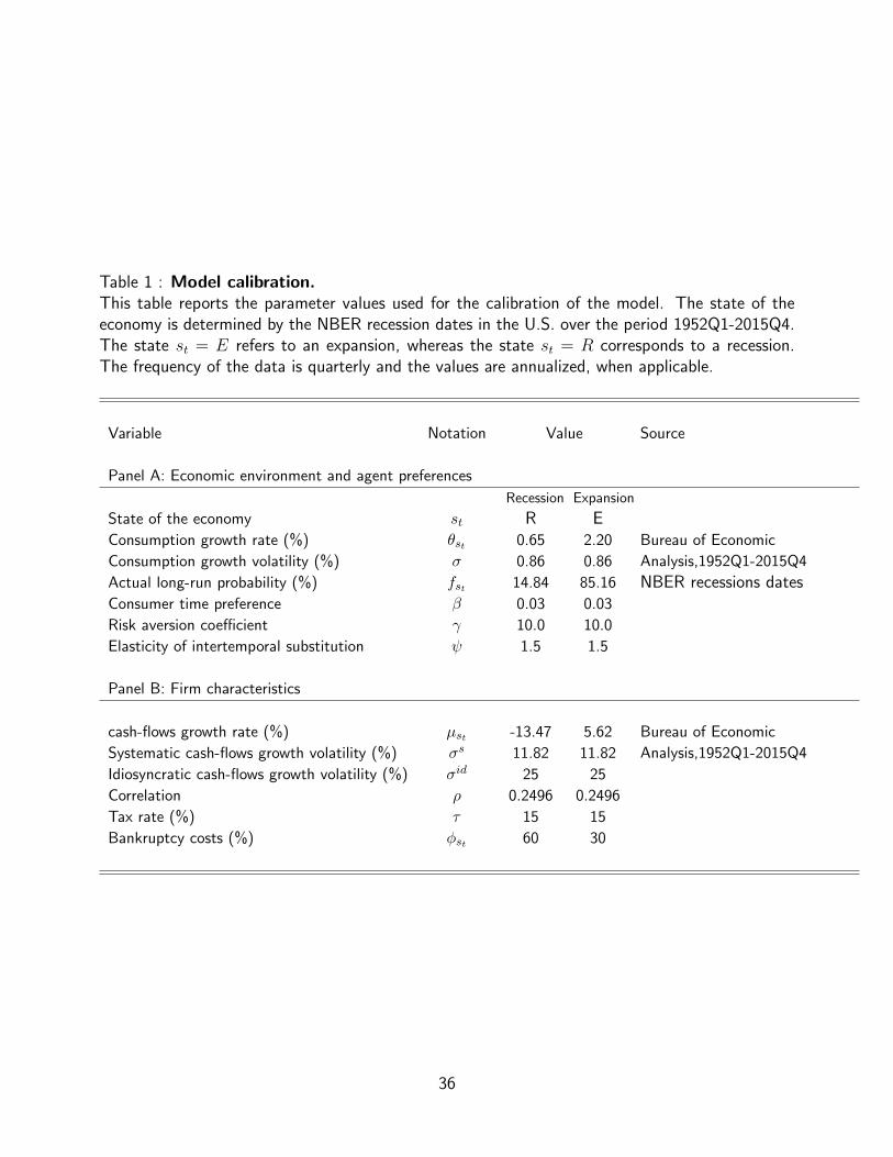
Table 1 : Model calibration.This table reports the parameter values used for the calibration of the model. The state of theeconomy is determined by the NBER recession dates in the U.S. over the period 1952Q1-2015Q4.The state st = E refers to an expansion, whereas the state st = R corresponds to a recession.The frequency of the data is quarterly and the values are annualized, when applicable.

Variable Notation Value Source

Panel A: Economic environment and agent preferences

Recession Expansion

State of the economy st R EConsumption growth rate (%) θst 0.65 2.20 Bureau of Economic

Analysis,1952Q1-2015Q4Consumption growth volatility (%) σ 0.86 0.86

Actual long-run probability (%) fst 14.84 85.16 NBER recessions datesConsumer time preference β 0.03 0.03

Risk aversion coefficient γ 10.0 10.0

Elasticity of intertemporal substitution ψ 1.5 1.5

Panel B: Firm characteristics

cash-flows growth rate (%) µst -13.47 5.62 Bureau of Economic

Analysis,1952Q1-2015Q4Systematic cash-flows growth volatility (%) σs 11.82 11.82

Idiosyncratic cash-flows growth volatility (%) σid 25 25

Correlation ρ 0.2496 0.2496

Tax rate (%) τ 15 15

Bankruptcy costs (%) φst 60 30

36

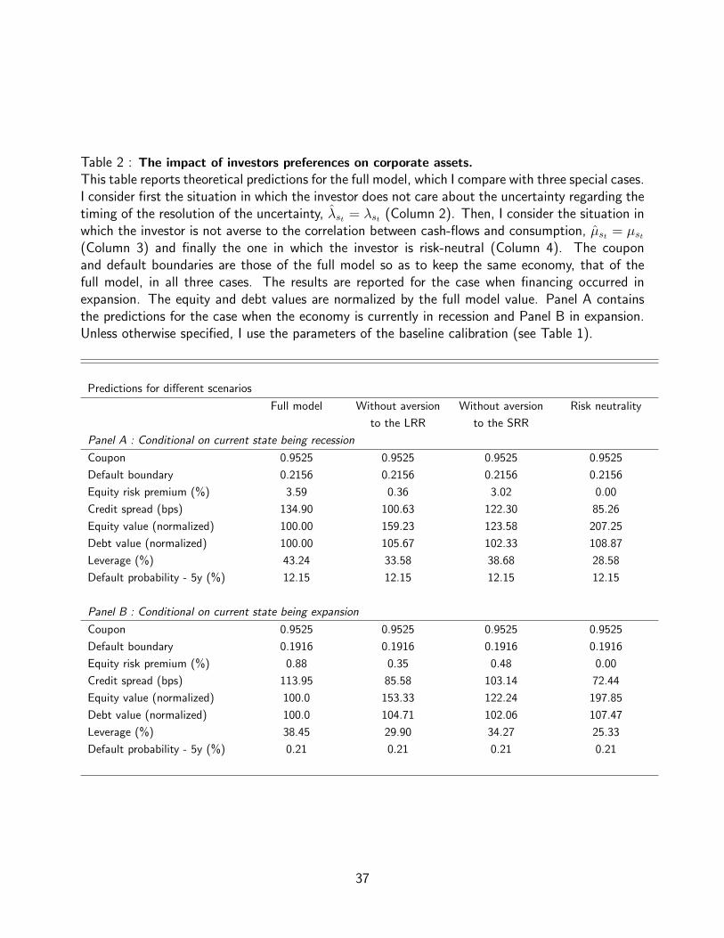
Table 2 : The impact of investors preferences on corporate assets.

This table reports theoretical predictions for the full model, which I compare with three special cases.I consider first the situation in which the investor does not care about the uncertainty regarding thetiming of the resolution of the uncertainty, λst = λst (Column 2). Then, I consider the situation inwhich the investor is not averse to the correlation between cash-flows and consumption, µst = µst(Column 3) and finally the one in which the investor is risk-neutral (Column 4). The couponand default boundaries are those of the full model so as to keep the same economy, that of thefull model, in all three cases. The results are reported for the case when financing occurred inexpansion. The equity and debt values are normalized by the full model value. Panel A containsthe predictions for the case when the economy is currently in recession and Panel B in expansion.Unless otherwise specified, I use the parameters of the baseline calibration (see Table 1).

Predictions for different scenarios

Full model Without aversion

to the LRR

Without aversion

to the SRR

Risk neutrality

Panel A : Conditional on current state being recession

Coupon 0.9525 0.9525 0.9525 0.9525

Default boundary 0.2156 0.2156 0.2156 0.2156

Equity risk premium (%) 3.59 0.36 3.02 0.00

Credit spread (bps) 134.90 100.63 122.30 85.26

Equity value (normalized) 100.00 159.23 123.58 207.25

Debt value (normalized) 100.00 105.67 102.33 108.87

Leverage (%) 43.24 33.58 38.68 28.58

Default probability - 5y (%) 12.15 12.15 12.15 12.15

Panel B : Conditional on current state being expansion

Coupon 0.9525 0.9525 0.9525 0.9525






Leverage (%) 38.45 29.90 34.27 25.33


37

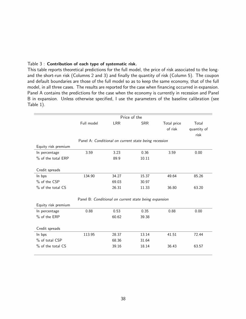
Table 3 : Contribution of each type of systematic risk.

This table reports theoretical predictions for the full model, the price of risk associated to the long-and the short-run risk (Columns 2 and 3) and finally the quantity of risk (Column 5). The couponand default boundaries are those of the full model so as to keep the same economy, that of the fullmodel, in all three cases. The results are reported for the case when financing occurred in expansion.Panel A contains the predictions for the case when the economy is currently in recession and PanelB in expansion. Unless otherwise specified, I use the parameters of the baseline calibration (seeTable 1).

Price of the

Full model LRR SRR Total price

of risk

Total

quantity of

risk

Panel A: Conditional on current state being recession

Equity risk premium

In percentage 3.59 3.23 0.36 3.59 0.00

% of the total ERP 89.9 10.11

Credit spreads

In bps 134.90 34.27 15.37 49.64 85.26

% of the CSP 69.03 30.97

% of the total CS 26.31 11.33 36.80 63.20

Panel B: Conditional on current state being expansion

Equity risk premium

In percentage 0.88 0.53 0.35 0.88 0.00

% of the ERP 60.62 39.38

Credit spreads

In bps 113.95 28.37 13.14 41.51 72.44

% of total CSP 68.36 31.64

% of the total CS 39.16 18.14 36.43 63.57

38

Table 4 : Risk aversion, equity risk premium and credit spread.

This table reports theoretical predictions for the full model, which I compare with three specialcases. I consider first the case in which the investor does not care about the uncertainty regardingthe timing of the resolution of the uncertainty, i.e. λst = λst (Column 2). Then, I consider amodel in which the investor is not averse to the correlation between cash-flows and consumption,i.e. µst = µst (Column 3) and finally a model in which the investor is risk-neutral (Column 4).The coupon and default boundaries are those of the full model so as to keep the same economy,that of the full model, in all three cases. Panel A report the credit spread (Panel A1) and equityrisk premium (panel A2) obtained for two different levels of risk aversion, high, γ = 14 and low,

γ = 2 that I compare with the baseline predictions and the Panel B the contribution of each type ofsystematic risk. The results are reported for the case when financing occurs in expansion (s0 = E).Equity risk premiums and credit spreads are weighted average, where the weights are given by theactual long-run distribution, fst . Unless otherwise specified, I use the parameters of the baselinecalibration (see Table 1).

Panel A: Equity risk premium and credit spreadFull model

(A)Without aversion

to LRR

(B)

Without aversionto SRR

(C)

Risk neutrality

(D)

Panel A1: Equity risk premium (pct)

Low CRRA 0.171 0.068 0.102 0.00

Baseline 1.282 0.349 0.855 0.00

High CRRA 2.026 0.496 1.351 0.00

Panel A2: Credit spread (bps)

Low CRRA 82.81 78.63 80.17 75.87

Baseline 117.06 87.81 105.98 74.34

High CRRA 135.14 92.21 120.28 73.53

Panel B : Decomposition of the price of risk

Price of LRR

(A) - (B)Price of SRR

(A) - (C)Total

(A) - (D)Panel B1: Equity risk premium (pct)

Low CRRA 0.104 0.068 0.171

Baseline 0.933 0.349 1.282

High CRRA 1.530 0.496 2.026

Panel B2: Credit spread premium (bps)

Low CRRA 4.18 2.76 6.94

Baseline 29.25 13.47 42.71

High CRRA 42.93 18.68 61.61

39

Table 5 : EIS coefficient, equity risk premium and credit spread.

This table reports theoretical predictions for the full model, which I compare with three specialcases. I consider first the case in which the investor does not care about the uncertainty regardingthe timing of the resolution of the uncertainty, i.e. λst = λst (Column 2). Then, I consider amodel in which the investor is not averse to the correlation between cash-flows and consumption,i.e. µst = µst (Column 3) and finally a model in which the investor is risk-neutral (Column 4).The coupon and default boundaries are those of the full model so as to keep the same economy,that of the full model, in all three cases. Panel A report the credit spread (Panel A1) and equityrisk premium (panel A2) obtained for two different levels of EIS coefficient, high, ψ = 2.5 and low,

ψ = 0.5 that I compare with the baseline predictions and the Panel B the contribution of eachtype of systematic risk. The results are reported for the case when financing occurs in expansion(s0 = E). Equity risk premiums and credit spreads are weighted average, where the weights aregiven by the actual long-run distribution, fst . Unless otherwise specified, I use the parameters ofthe baseline calibration (see Table 1).


(A)Without aversion

to LRR

(B)


(C)

Risk neutrality

(D)


Low EIS 1.557 0.484 0.975 0.00

Baseline 1.282 0.349 0.855 0.00

High EIS 1.228 0.324 0.829 0.00


Low EIS 123.45 105.52 116.39 98.88

Baseline 117.06 87.81 105.98 74.34

High EIS 109.04 69.31 94.51 44.65


Price of LRR


(A) - (C)Total


Low EIS 1.073 0.484 1.557

Baseline 0.933 0.349 1.282

High EIS 0.904 0.324 1.228


Low EIS 17.92 6.64 24.56

Baseline 29.25 13.47 42.71

High EIS 39.72 24.66 64.39

40

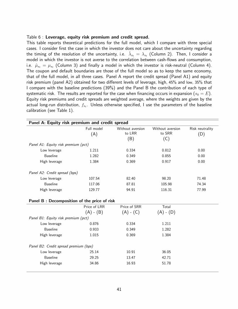
Table 6 : Leverage, equity risk premium and credit spread.

This table reports theoretical predictions for the full model, which I compare with three specialcases. I consider first the case in which the investor does not care about the uncertainty regardingthe timing of the resolution of the uncertainty, i.e. λst = λst (Column 2). Then, I consider amodel in which the investor is not averse to the correlation between cash-flows and consumption,i.e. µst = µst (Column 3) and finally a model in which the investor is risk-neutral (Column 4).The coupon and default boundaries are those of the full model so as to keep the same economy,that of the full model, in all three cases. Panel A report the credit spread (Panel A1) and equityrisk premium (panel A2) obtained for two different levels of leverage, high, 45% and low, 35% thatI compare with the baseline predictions (39%) and the Panel B the contribution of each type ofsystematic risk. The results are reported for the case when financing occurs in expansion (s0 = E).Equity risk premiums and credit spreads are weighted average, where the weights are given by theactual long-run distribution, fst . Unless otherwise specified, I use the parameters of the baselinecalibration (see Table 1).


(A)Without aversion

to LRR

(B)


(C)

Risk neutrality

(D)


Low leverage 1.211 0.334 0.812 0.00

Baseline 1.282 0.349 0.855 0.00

High leverage 1.384 0.369 0.917 0.00


Low leverage 107.54 82.40 98.20 71.48

Baseline 117.06 87.81 105.98 74.34

High leverage 129.77 94.91 116.31 77.99


Price of LRR


(A) - (C)Total


Low leverage 0.876 0.334 1.211

Baseline 0.933 0.349 1.282

High leverage 1.015 0.369 1.384


Low leverage 25.14 10.91 36.05

Baseline 29.25 13.47 42.71

High leverage 34.86 16.93 51.78

41

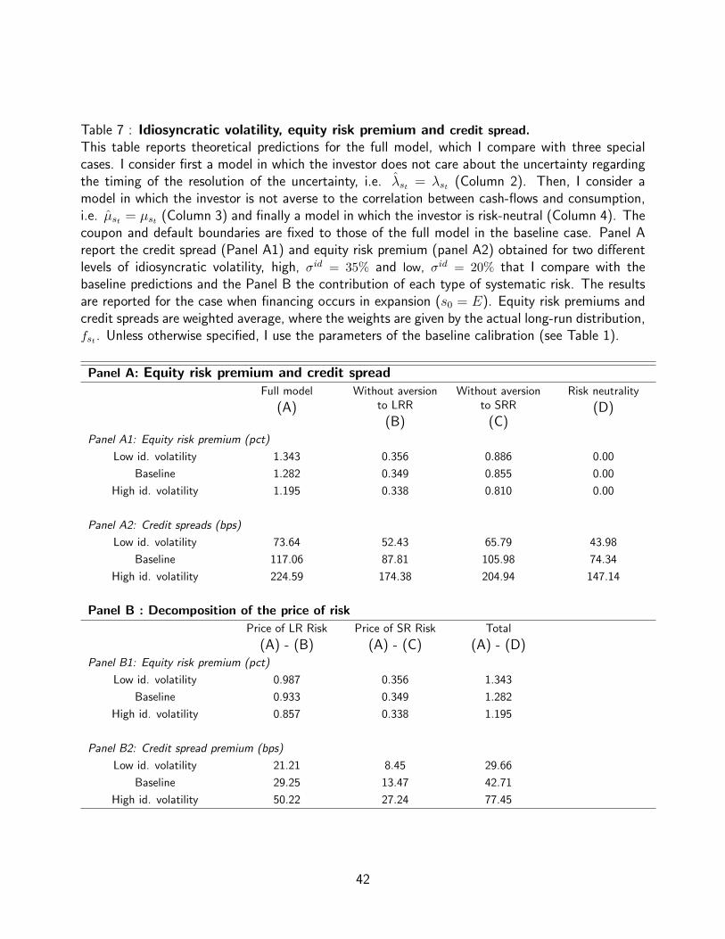
Table 7 : Idiosyncratic volatility, equity risk premium and credit spread.

This table reports theoretical predictions for the full model, which I compare with three specialcases. I consider first a model in which the investor does not care about the uncertainty regardingthe timing of the resolution of the uncertainty, i.e. λst = λst (Column 2). Then, I consider amodel in which the investor is not averse to the correlation between cash-flows and consumption,i.e. µst = µst (Column 3) and finally a model in which the investor is risk-neutral (Column 4). Thecoupon and default boundaries are fixed to those of the full model in the baseline case. Panel Areport the credit spread (Panel A1) and equity risk premium (panel A2) obtained for two differentlevels of idiosyncratic volatility, high, σid = 35% and low, σid = 20% that I compare with thebaseline predictions and the Panel B the contribution of each type of systematic risk. The resultsare reported for the case when financing occurs in expansion (s0 = E). Equity risk premiums andcredit spreads are weighted average, where the weights are given by the actual long-run distribution,fst . Unless otherwise specified, I use the parameters of the baseline calibration (see Table 1).


(A)Without aversion

to LRR

(B)


(C)

Risk neutrality

(D)


Low id. volatility 1.343 0.356 0.886 0.00

Baseline 1.282 0.349 0.855 0.00

High id. volatility 1.195 0.338 0.810 0.00

Panel A2: Credit spreads (bps)

Low id. volatility 73.64 52.43 65.79 43.98

Baseline 117.06 87.81 105.98 74.34

High id. volatility 224.59 174.38 204.94 147.14


Price of LR Risk

(A) - (B)Price of SR Risk

(A) - (C)Total


Low id. volatility 0.987 0.356 1.343

Baseline 0.933 0.349 1.282

High id. volatility 0.857 0.338 1.195


Low id. volatility 21.21 8.45 29.66

Baseline 29.25 13.47 42.71

High id. volatility 50.22 27.24 77.45

42

Table 8 : The impact of investors preferences on corporate assets - Endogenous policy.

This table reports theoretical predictions for the full model, which I compare with three specialmodels. I consider first a model in which the investor does not care about the uncertainty regardingthe timing of the resolution of the uncertainty, λst = λst (Column 2). Then, I consider a model inwhich the investor is not averse to the correlation between cash-flows and consumption, µst = µst(Column 3) and finally a model in which the investor is risk-neutral (Column 4). The coupon anddefault boundaries are endogenous, i.e., shareholders now consider investors preferences in theirdecision making. The results are reported for the case when financing occurred in expansion. Theequity and debt values are normalized by the full model value. Panel A contains the predictions forthe case when the economy is currently in recession and Panel B in expansion. Unless otherwisespecified, I use the parameters of the baseline calibration (see Table 1).

Predictions for different economies

Full model

When agent is

averse to the

SRR

When agent is

averse to the LRRRisk neutrality


Coupon 0.9525 1.3702 1.1009 1.6771






Leverage (%) 43.24 45.52 43.70 45.99

Equity return volatility (%) 51.46 52.17 51.88 52.62



Coupon 0.9525 1.3702 1.1009 1.6771






Leverage (%) 38.45 40.84 38.84 41.25

Equity return volatility (%) 42.22 43.52 42.47 43.81


43

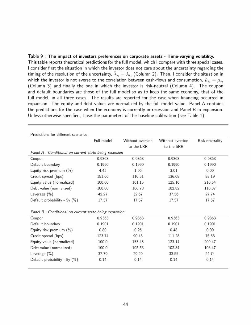
Table 9 : The impact of investors preferences on corporate assets - Time-varying volatility.

This table reports theoretical predictions for the full model, which I compare with three special cases.I consider first the situation in which the investor does not care about the uncertainty regarding thetiming of the resolution of the uncertainty, λst = λst (Column 2). Then, I consider the situation inwhich the investor is not averse to the correlation between cash-flows and consumption, µst = µst(Column 3) and finally the one in which the investor is risk-neutral (Column 4). The couponand default boundaries are those of the full model so as to keep the same economy, that of thefull model, in all three cases. The results are reported for the case when financing occurred inexpansion. The equity and debt values are normalized by the full model value. Panel A containsthe predictions for the case when the economy is currently in recession and Panel B in expansion.Unless otherwise specified, I use the parameters of the baseline calibration (see Table 1).

Predictions for different scenarios

Full model Without aversion

to the LRR

Without aversion

to the SRR

Risk neutrality


Coupon 0.9363 0.9363 0.9363 0.9363






Leverage (%) 42.27 32.67 37.56 27.74



Coupon 0.9363 0.9363 0.9363 0.9363






Leverage (%) 37.79 29.20 33.55 24.74


44

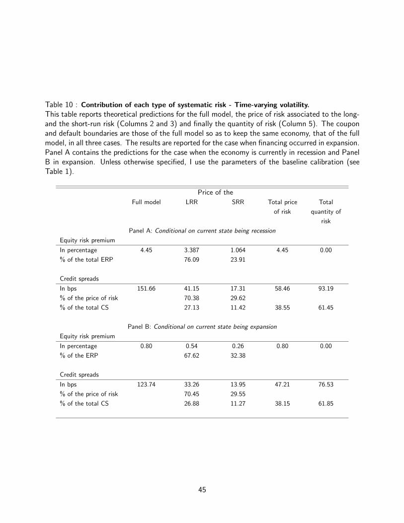
Table 10 : Contribution of each type of systematic risk - Time-varying volatility.


Price of the

Full model LRR SRR Total price

of risk

Total

quantity of

risk

Panel A: Conditional on current state being recession

Equity risk premium

In percentage 4.45 3.387 1.064 4.45 0.00

% of the total ERP 76.09 23.91

Credit spreads

In bps 151.66 41.15 17.31 58.46 93.19

% of the price of risk 70.38 29.62

% of the total CS 27.13 11.42 38.55 61.45

Panel B: Conditional on current state being expansion

Equity risk premium

In percentage 0.80 0.54 0.26 0.80 0.00

% of the ERP 67.62 32.38

Credit spreads

In bps 123.74 33.26 13.95 47.21 76.53

% of the price of risk 70.45 29.55

% of the total CS 26.88 11.27 38.15 61.85

45

Table 11 : Impact of the time-varying volatility in risk premia.


In recession In expansionTotal LRR impact Total LRR impact

Equity risk premium % Proportion % Proportion

T-V growth and volatility 4.45 76.1% 0.80 67.6%

T-V growth only 3.59 89.9% 0.88 60.6%

Credit spreads premium bps Proportion % Proportion

T-V growth and volatility 58.46 70.4% 47.21 70.5%

T-V growth only 49.64 69.1% 41.51 68.4%

46

Appendix

I present the main point of the model which is a static version of the model of Bhamra, Kuehn, and

Strebulaev (2010a, b). The model uses a state-dependent approach to derive endogenously each

state optimum coupon and default boundaries which in turn are used to compute the firms claims,

i.e. equity and debt. The Arrow-Debreu default claims which measure the present value of the

jump in the state-price density from one state to another allow to introduce the state-dependency

in the pricing.

A Consumption and cash-flows dynamics

The economy is populated by the N firms and a representative agent. Firm cash-flows vary with

continuous shocks and time-varying macroeconomic conditions. All variables are in real terms.

A.1 Consumption

Let Ct denote the perpetual stream of consumption in the economy. The output level follows the

process

dCtCt

= θstdt+ σstdBt, st = {R,E} , (11)

where θst and σst are the drift and volatility of output, and Bt is a standard Brownian motion

under the physical measure.

This economy is characterized by the long-run risk, which creates variation in the business cycle.

I assume that the economy is governed by two states such that the first and second moments of

output growth, θst and σst , are state-dependent. The state of the economy at time t is determined

by st, which is equal to R in recession and to E in expansion. The first moment is procyclical,

while the second one is countercyclical such that θE > θR and σE < σR. The evolution of st is

given by a 2-state Markov chain. All agents can observe the current state of the economy.

47

A.2 Firm cash-flows

The firm i has a stream of cash-flows, denoted by Xi,t, which is given by

dXi,t

Xi,t

= µi,stdt+ σidi dBidi,t + σsi,stdBt, st = {R,E} , (12)

where µi,st is the conditional growth rate of the firm i’s cash-flows, while σidi and σgi

capture

respectively the idiosyncratic and systematic volatility of the firm i’s earning growth rate. The

standard Brownian motion Bidi,t is the shock specific to firm i, which is uncorrelated to the shock

to consumption Bt. The firm i’s total earning volatility is equal σXi,st =√(

σidi)2

+(σgi,st

)2. The

procyclical nature of economic growth implies that µi,E > µi,R.

The firms’ cash-flows depend on the macroeconomic environment in two ways. First, all firms share

common shocks coming from the country level economic conditions. As consequence, firm cash-

flows shocks are correlated with the shocks to the aggregate consumption, so that: dBtdBC,t = ρdt,

where ρ is the constant coefficient of correlation between cash-flows and consumption. Second,

the firms cash-flows follow the business cycle, which is determined by the state st.

B State-price density and equilibrium risk-free rate

In this section, I provide the formula of the state-price density and the equilibrium risk-free rate.17

The state-price density is initially derived by Duffie and Skiadas (1994) for the general class of

stochastic differential utility function proposed by Duffie and Epstein (1992). This type of utility

function incorporates not only the agent’s risk aversion but also the aversion for intertemporal

resolution of the uncertainty in the economy.

The representative agent’s state-price density πt, in the case ψ 6= 1, is given by

πt =(βe−βt

) 1−γ

1− 1ψ C−γt

(pC,ste

∫ t0 p−1C,su

du)− γ− 1

ψ

1− 1ψ , (13)

17For additional details and complete derivation, I refer the reader to the Appendix of Bhamra, Kuehn, andStrebulaev (2010b) in the case of two states, and to the Appendix of Chen (2010) for N states.

48

where pC,st is the price-consumption ratio that satisfies the following implicit non-linear equation:

p−1C,st = rst − θst + γσ2st −(

1− 1

ψ

)λst

(pC,stpC,st

) 1−γ1− 1

ψ − 1

1− γ

, st, st ∈ {R,E} , st 6= st (14)

with

rst = β +1

ψθst −

1

2γ

(1 +

1

ψ

)σ2st . (15)

The dynamics of the state-price density πt follow the following stochastic differential equation

dπtπt

= −rstdt+dMt

Mt

(16)

= −rstdt−ΘBstdBt + ΘP

stdNst,t, (17)

where M is a martingale under the physical measure, Nst,t a Poisson process which jumps upward

by one whenever the state of the economy switches from st to st 6= st, ΘBst = γσ2

st is the market

price of risk due to Brownian shocks in state st, and ΘPst = ∆st − 1 is the market price of risk due

to Poisson shocks when the economy switches out of state st = {R,E}.

Finally, rst represents the equilibrium real risk-free rate, which is given by

rst =

rL + λL

[γ− 1

ψ

1−γ

(∆− γ−1

γ− 1ψ − 1

)− (∆−1 − 1)

], st = R

rH + λH

[γ− 1

ψ

1−γ

(∆

γ−1

γ− 1ψ − 1

)− (∆− 1)

], st = E

(18)

with ∆H = ∆−1L = ∆, where ∆ is the solution of G(∆) = 0 from

G(x) = x−

1− 1ψ

γ− 1ψ −

rH + γσ2H − θH + λH

1− 1ψ

γ−1

(xγ−1

γ− 1ψ − 1

)rL + γσ2

L − θL + λL1− 1

ψ

γ−1

(x− γ−1

γ− 1ψ − 1

) , ψ 6= 1 (19)

The agent has preference for earlier resolution of uncertainty in the case when γ > 1ψ

and thus

49

cares about the rate of news arrival, denoted by p. When p is small, the speed at which information

arrives is low, thereby increasing the risk of the intertemporal substitution for an agent averse to

such risk. The rate at which the distribution for the state of the economy converges to its steady

state is given by p = λR +λE, where λst is the probability per unit of time of leaving state st. The

quantity 1/λst is the expected duration of state st. Recessions are shorter than expansions, such

that 1/λR < 1/λE.

The physical probabilities λR and λE are converted to their risk-neutral counterparts λR and λE

through a risk distortion factor ∆E, which is defined as the change in the state-price density πt at

the transition time from expansion to recession. The risk-neutral probabilities per unit of time of

changing state are then given by

λE = ∆EλE and λR =1

∆E

λR. (20)

The agent prefers earlier resolution of the uncertainty, which implies that ∆E > 1. Hence, this

agent prices securities as if recessions last longer (λR > λR) and expansions shorter (λE < λE)

than in reality. The risk-neutral rate of news arrival is p = λR+ λE, which implies that the long-run

risk-neutral distribution is determined by(fR, fE

)=(λEp, λRp

).

The equilibrium risk-free rate prevailing in equilibrium in state st is given by (see Appendix A)

rst = rst −

(γ − 1

ψ

γ − 1

)λst

(1−∆

γ−1

γ− 1ψ

st

)+ λst (1−∆st) , ψ 6= 1, st = {R,E} , (21)

where

rst = β +1

ψθst −

1

2γ

(1 +

1

ψ

)σ2st . (22)

Higher uncertainty (σE < σR) and lower economic growth (θE > θR) in recession induce greater

demand for the risk-free bond, thereby reducing the equilibrium interest rate (rE > rR). The

risk-free interest rate is therefore procyclical.

50

C Arrow-Debreu default claims

This Appendix derives two kinds of Arrow-Debreu claims that are used to discount cash flows. The

first kind captures the default triggered by the firm’s earning falling below the default boundary,

whereas the second kind additionally accounts for the default related to a change in the state of

the economy. In the second case, default can occur instantaneously because of a change in state

although the firm’s earning remains unchanged. This situation can occur when the economy is in

good economic state (st = E) and switches to the bad state (sD = R), and the firm’s earning is

above the good state’s default boundary, but below the bad state’s default boundary. The reason

is that the default boundary is countercyclical (XD,R > XD,E), as shown in Bhamra, Kuehn, and

Strebulaev (2010a, p.4238). The first kind of the Arrow-Debreu claims is defined as

qstsD = Et

[πtDπtProb (sD | st) | st

], (23)

while the second kind corresponds to

q′stsD = Et

[πtDπt

XtD

Xst

Prob (sD | st) | st]. (24)

C.1 First kind

The Arrow-Debreu default security qstsD is the present time t value of a security that pays one unit

of consumption at the moment of default tD, where st represents the present state of the economy,

and sD the state at the default time. The time of default is the first time that the earning level of

the firm falls to the boundary XD,sD . By definition, this Arrow-Debreu claim is given by

qstsD = Et

[πtDπtProb (sD | st) | st

], (25)

which is solution of the two ordinary differential equations (ODE)

1

2σ2i,stX

2d2qstsDdX2

+ µstXdqD,stsDdX

+λst (qjsD − qstsD)− rstqstsD = 0, st = {R,E} , (26)

51

where σi,st denotes the firm’s earning growth volatility in state st.

The above ODEs are obtained by applying Ito’s Lemma to the classical non-arbitrage condition

EQt [dqstsD − rstqstsD ] = 0, (27)

The Arrow-Debreu claim payoffs are such that:

qstsD (X) =

1, st = sD, X ≤ XD,st

0, st 6= sD, X ≤ XD,st .

, st, sD = {R,E} (28)

Therefore, each state of the economy is characterized by a specific default boundary. The default

barriers are higher in recession and lower in expansion, that is XD,E ≤ XD,R. Each of the four

Arrow-Debreu claims is then determined over three separate intervals: X ≥ XD,R, XD,R ≥ X ≥

XD,E, and X ≤ XD,E.

From the payoff equations, I can infer the values of the four Arrow-Debreu claims in the interval

X ≤ XD,E. For the interval X ≥ XD,R, I are looking for a solution of the following general form:

qstsD (X) = hstsDXk, (29)

which implies that k must be a root of the quartic equation

[1

2σ2i,Ek (k − 1) + µRk +

(−λR − rR

)] [1

2σ2i,Ek (k − 1) + µEk +

(−λE − rE

)]−λRλE = 0. (30)

The Arrow-debreu claims can be written as

qstsD (X) =4∑

m=1

hstsDmXkm (31)

with k1, k2 < 0 and k3, k4 > 0. However, when Y goes to infinity the Arrow-Debreu claims must

52

be null, which indicates that I should have hstsD,3 = hstsD,4 = 0. I then obtain

qRsD (Y ) =2∑

m=1

hRsD,mXkm (32)

qEsD (Y ) =2∑

m=1

hEsD,mε (km)Xkm , (33)

where

ε (km) = − λH12σ2i,Hk (k − 1) + µEk −

(λE + rE

) = −12σ2i,Rk (k − 1) + µRk −

(λR + rR

)λR

. (34)

Finally, over the interval XD,R ≥ X ≥ XD,E, both qD,RR and qD,RE are known from the payoffs

equations and are respectively equal to 1 and 0. Then,

qER (X) =λE

rE + λE+

2∑m=1

sR,mXjm (35)

qEE (X) =2∑

m=1

sE,mXjm , (36)

where1

2σ2i,Ej (j − 1) + µRj −

(λE + rE

)= 0 (37)

with j1 < j2.

53

To summarize, the four Arrow-Debreu claims can be written as follows

qRR =

∑2m=1 hRR,mX

km , X ≥ XD,R

1, XD,R ≥ X ≥ XD,E

1, X ≤ XD,E

(38)

qRE =

∑2m=1 hRE,mX

km , X ≥ XD,E

0, XD,R ≥ X ≥ XD,E

0, X ≤ XD,E

(39)

qER =

∑2m=1 hRR,mε (km)Xkm , X ≥ XD,R

λErE+λE

+∑2

m=1 sR,mXjm , XD,R ≥ X ≥ XD,E

0, X ≤ XD,E

(40)

qEE =

∑2m=1 hRE,mε (km)Xkm , X ≥ XD,R∑2m=1 sE,mX

jm , XD,R ≥ X ≥ XD,E

1, X ≤ XD,E.

(41)

The eight constants are determined by eight boundary conditions, which are

limX→XD,R

qEE = 1, limX→XD,R

qRE = 0 (42)

limX→X+

D,R

qER = limX→X−D,R

qER, limX→X+

D,R

qEE = limX→X−D,R

qEE (43)

limX→X+

D,R

qER = limX→X−D,R

qER, limX→X+

D,R

qEE = limX→X−D,R

qEE (44)

limX→XD,E

qER = 0, limX→XD,E

qEE = 1. (45)

C.2 Second kind

I use the same approach to derive the second kind of Arrow-Debreu default claims, which account

for the possibility that a default can when the state of the economy changes. The only claim that

54

is different from that of the first kind is qHL, whose expression is now given by

q′

ER =

∑2m=1 hRR,mε (km)Xkm , X ≥ XD,R

λErE+λE−µE

XXD,R

+∑2

m=1 sR,mXjm , XD,R ≥ X ≥ XD,E

0, X ≤ XD,E.

(46)

D Corporate debt

The present debt value, Dst , is the discounted perpetual coupon stream before default s plus the

present value of the after-tax firm recovered asset value at default. Hence, the debt value is:

Dst = Et

[∫ tD

t

cπuπtdu | st

]+ Et

[πuπtφtDAtDdu | st

](47)

=c

rB,st−∑sD

(c

rB,sD− φtDAtD

)qstsD , st, sD = {R,E} (48)

where φst is the state-dependent asset recovery rate, Ast = (1 − τ) XrA,st

is the firm asset

liquidation value, rB,st = rst +rj−rstp+rj

pfj, j 6= st is the bond discount rate and rA,st = rst − µst +

(rj−µj)−(rst−µst)p+rj−µj pfj, j 6= st, is the risky discount rate with µst = µst − γρσgstσst .

E Equity value

The equity value, Sst , is the after-tax discounted value of future cash-flows (i.e. EBIT) less coupon

payments before bankruptcy is declared by the stockholders

Sst = (1− τ)Et

[∫ tD

t

πuπt

(Xt − c) du | st], st = {R,E} ,

hence

55

Sst = AtD − (1− τ)c

rB,st−∑sD

((1− τ)

c

rB,sD− AtD

)qstsD , st, sD = {R,E} (49)

where AtD is the asset recovery rate at the time the shareholders decide to declare bankruptcy

(see section D).

F Estimation of the transition probabilities

This section describes the estimation of the transition probabilities considered in the paper. I

estimate a Markov regime-switching model with two regimes using the NBER recession dates over

the period 1952Q1-2015Q4. The transition probability matrix, is obtained by maximum likelihood

using the Hamilton (1989)’s approach. There are some issues with the estimation when using

consumption date between of the period spanning the 2007-09 financial crisis. This originates

from the fact that the consumption growth slowdown was so pronounced during this period that

it is recognized as representing by itself one more regime. To overcome that, I have replaced the

consumption data by the NBER dates and put 1 or 0 when the economy is respectively in recession

or in expansion. The estimation gives the following transition matrix:

T =

TRR TRE

TER TEE

= T =

0.9603 0.2275

0.0397 0.7725

(50)

where Tij denotes the probability of a switch from state i to state j.

The actual long-run probability fst to be in the state st ∈ {R,E} is determined by fR =(1 + TRE

TER

)−1and fE = 1− fR. The probability λst that the economy leaves the state st ∈ {R,E}

is then given by λR = pfE and λE = pfR, with p = −4ln(

1− TRE1−fR

).

56

what drives corporate asset prices: short- or long-run risk?

Documents