what drives long-run biodiversity change? new … drives long... · what drives long-run...
TRANSCRIPT
What drives long-run biodiversity change? New insights from
combining economics, paleoecology and environmental history.
Nick Hanley and Dugald Tinch, Economics Department, University of Stirling;
Konstantinos Angelopoulos, Economics Department, University of Glasgow;
Althea Davies, School of Biological and Environmental Sciences, University of Stirling;
Edward B. Barbier, Dept. of Economics and Finance, University of Wyoming.
Fiona Watson, History Department, University of Dundee, Scotland;
Address for correspondence: Nick Hanley, Economics Department, University of Stirling,
Stirling FK9 4LA, Scotland, UK. Email [email protected]. Phone +44 1786 466410. Fax
+44 1786 467469.
Running title: What drives biodiversity change?
We thank the Leverhulme Trust for funding the research on which this paper is based. We also
thank participants at the First Conference on Early Economic Developments, Copenhagen, 2006
for helpful comments, especially Gregory Clark, and participants at the Frontiers of
Environmental Economics conference, Washington DC, February 2007, especially Kerry Smith,
Spencer Banzhaf, and Glenn Harrison. Thanks to Alistair Hamilton and Alasdair Ross for
research assistance and to an anonymous referee, Elias Tzavalis, Chris Smout and Brian Huntley
for comments.
2
Abstract This paper presents a new approach to understanding the effects of economic factors on
biodiversity change over the long run. We illustrate this approach by studying the determinants of
biodiversity change in upland Scotland from 1600-2000. The measure of biodiversity used is a
proxy for plant species diversity, constructed using statistical analysis of paleoecological (pollen)
data. We assemble a new data set of historical land use and prices over 11 sites during this 400
year period; this data set also includes information on changes in agricultural technology, climate
and land ownership. A panel model is then estimated, which controls for both supply and demand
shifts over time. A main result is that prices, which act in our model as a proxy for livestock
numbers, do indeed impact on biodiversity, with higher prices leading to lower biodiversity.
Keywords: agricultural development, biodiversity, paleoecology, panel models, instrumental variables. JEL codes: C33, N53, O13, Q57
3
1. Introduction
The state of a nation’s “biodiversity” has emerged as an increasingly important indicator
of environmental health [49]. Biodiversity incorporates the range and abundance of plant and
animal species, the interactions between them, and the natural systems that support them [7].
Whilst many measures of biodiversity exist, the number of different species existing in a given
area is an important component of most indicators, and this is the concept used in this paper.
Biodiversity can be expected to change over time as ecosystems evolve, partly in response to
exogenous shocks. What interests us in this paper is quantifying the long-term relationship
between biodiversity (derived from pollen data) and the functioning of the economic system: in
particular, we focus on agricultural change as a potential driver of biodiversity change.
Threats to biodiversity from human activity are usually thought of by biologists in terms
of habitat loss, degradation, and fragmentation; harvesting; and human-induced climate change
[33]. Addressing these threats at both the theoretical and empirical level has been an important
theme in environmental economics work in the recent past, as evidenced for instance in work on
drivers of rainforest loss [9]. But at the empirical level, this work has been limited to looking
either at rather recent cross-sectional data (eg species loss by country) or at rather short-duration
time series data, typically looking no further back than the 1970s.
The main contribution of this paper is two-fold. First, we set out a new, empirical method
for investigating the drivers of biodiversity loss over time, in manner which allows for the
relative weights of economic, social and environmental factors to be judged. Second, we
assemble and analyze an illustrative data set which allows econometric modeling of one estimate
of biodiversity change (using pollen richness as a proxy for plant diversity) as a function of
economic development in an agricultural economy over a 400 year period for Scotland. This data
set is assembled using inputs from economic history and paleoecology for a sample of upland
4
sites. We estimate a structural model which is based on the dominant ecological theory about
what drives plant species change in the uplands of North-West Europe, namely changes in
grazing pressure from livestock [5], [34], [44]. Given the lack of historical data on livestock
numbers, we illustrate how livestock prices may be used instead of grazing pressure as a
determinant of long-term biodiversity impacts. We then test the findings of this main model using
a shorter panel with actual livestock densities, albeit at a less precise spatial level.
2. A new approach to modeling biodiversity change over the long run.
Contemporary economic analysis of the determinants of biodiversity change take it as a necessary
condition for analysis that a dataset on biodiversity indicators exists, which can be combined with
economic (e.g. prices), social (e.g. civil liberty measures) and environmental (e.g. climate) data in
an econometric analysis. This, for example, is the basis for the many studies on determinants of
rainforest loss summarized in Barbier and Burgess [9]. However, this kind of data on biodiversity
is typically rather modern – few time series or cross sections amenable to economic analysis exist
pre-20th century. Yet our understanding of the long-term process of biodiversity change would be
much enhanced if economists could look back further into the past, rather than relying on short-
run time series or cross sectional variation. Moreover, much of the debate on the restoration of
habitats and indeed water quality in North America and Europe is based on an ideal of returning
systems to “natural conditions” – by which is often meant “pre-anthropogenic” or “pre-
industrial” conditions [51]. Understanding the environmental past, and how economic forces
have helped shape these processes of change, can enrich our ability to inform contemporary
policy debates.
The disciplines of paleoecology and environmental history offer a route to understanding
past environmental change. Paleoecology is the science of reconstructing past environments
5
using sources such as pollen records found in lake sediments and peat bogs [29]. By identifying
plants from their pollen remains, and dating the sediments in which the pollen occurs, changes in
the distribution of vegetation and patterns of land-use around a given site can be reconstructed
through time. In our data, these pollen records stretch back to 5500 BP (years before present).
Paleoecological analysis has been combined with both archaeological techniques [17], [39] and
historical sources [21], [46], [47] to understand the environmental impacts of human land use.
The discipline of environmental history [30], [38] uses a range of sources, primarily
written sources, but also ecological and paleoecological data, to understand historic
environmental change, and has been increasingly applied in North America and Europe [52],
[41]. However, no attempt that the authors are aware of has been previously made to combine
paleoecological methods with a quantitative economic analysis of the determinants of land use
and land management intensity. This is the approach taken here: we use paleoecological methods
to estimate plant diversity over time for a range of sites, and then use historical analysis of
documentary sources to construct a database of candidate determinants of changes in the
biodiversity measure which are informed by an economic model of land use. Finally, panel data
econometric methods are used to examine this combined data-base.
The example we use to illustrate this approach is the use of upland grazing in Scotland,
over the period 1600-2000. The measure of biodiversity extracted from the paleoecological
record is the standardized number of pollen types observed at each site i in each time period t.
Based on current ecological understanding of how grazing pressure from livestock relates to plant
diversity at upland sites , we expect that sheep and cattle stocking decisions will impact on this
estimate of plant diversity over time. In what follows, we first explain how the database for the
case study was created, before detailing the econometric analysis undertaken. In the Conclusions
section, we comment on other contexts in which this “new approach” can be applied.
6
3. Data collection
Virtually all of the data used in this application had to be obtained from primary
documentary sources and new paleoecological investigations by the research team. The first
requirement was to select the sites to be used for data collection. Sites were intended to represent
a range of biogeographical zones in the Scottish uplands, from the hills of the Scottish borders to
the northernmost areas on the mainland (note that sites were not sampled on the basis of expected
biodiversity levels0F
i). This was an iterative process, involving identifying sites with historical
potential (i.e. sites where there was a reasonable chance of obtaining enough, intact primary
documentary sources), alongside fieldwork to seek suitable peat deposits (to obtain intact,
undisturbed historic pollen sequences), and then final joint site selection.
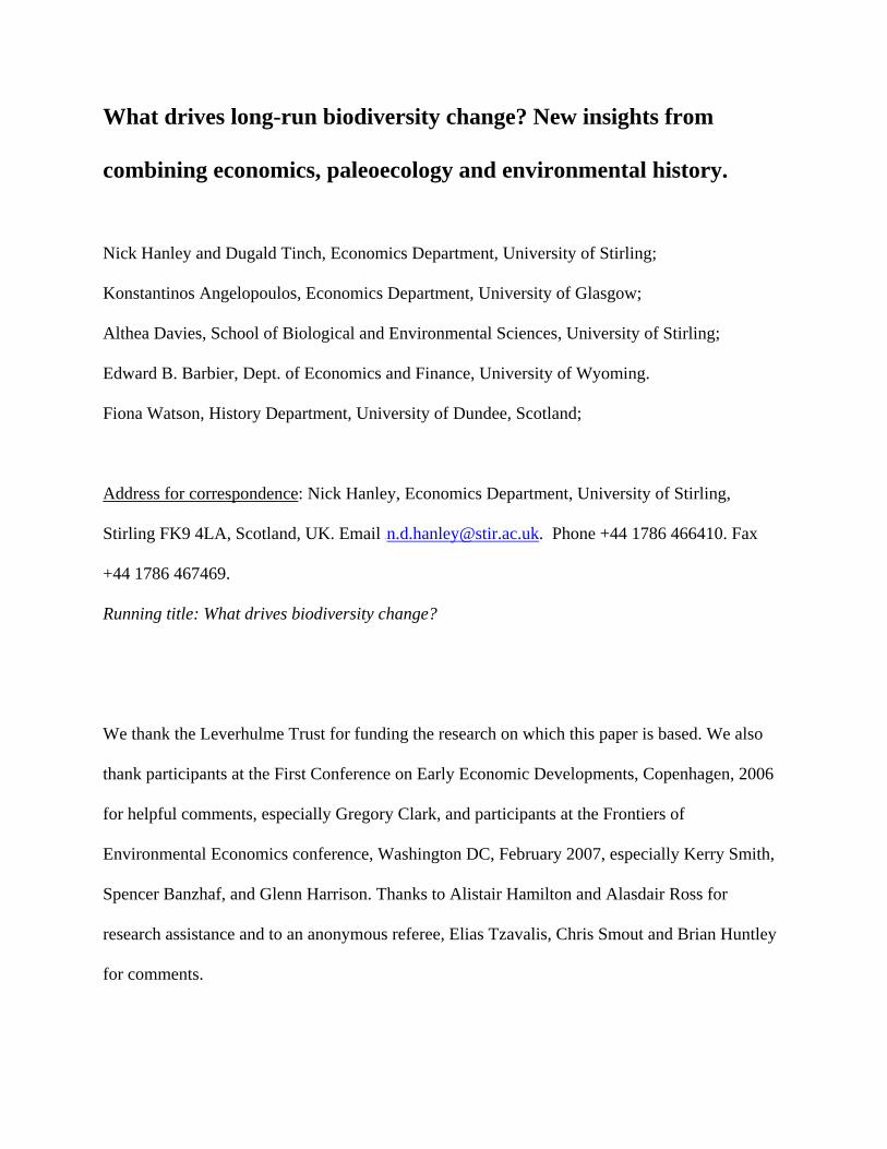
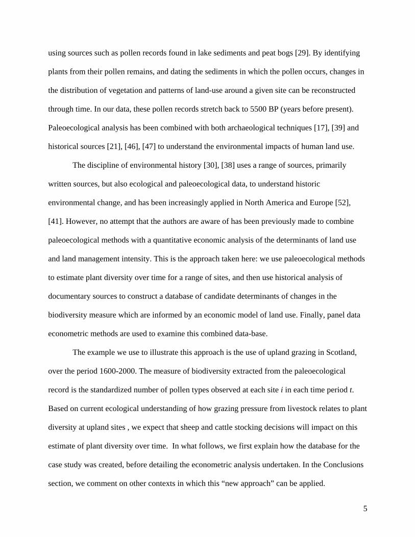
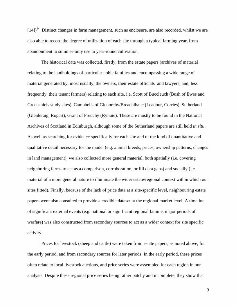
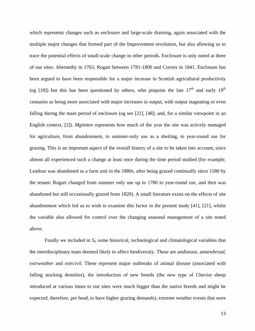
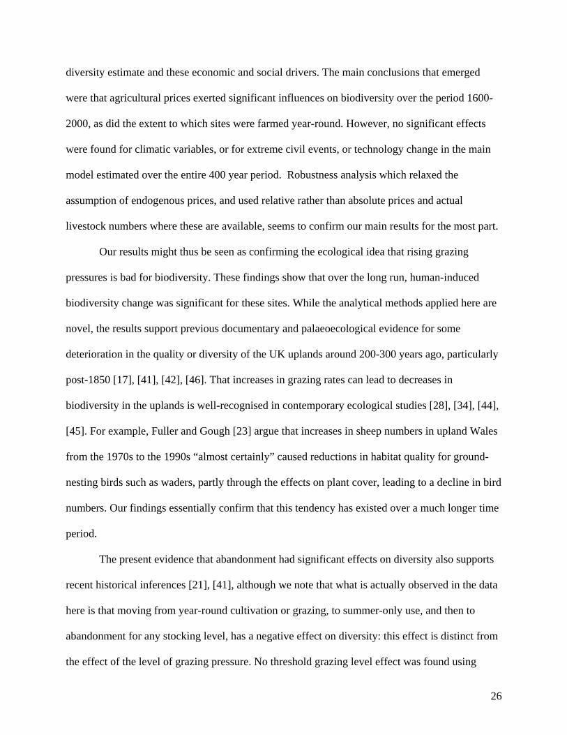
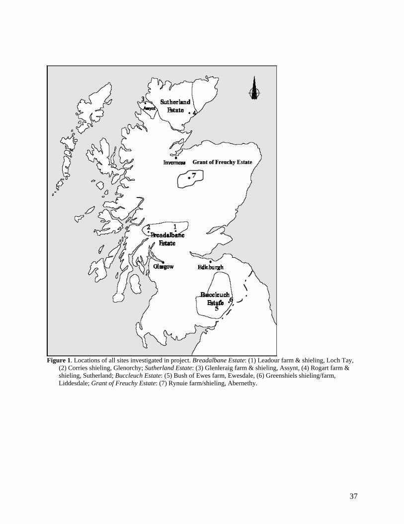
The eleven sites eventually selected are shown in Figure One. They include two sites in
the Southern Uplands (Greenshiels and Bush of Ewes), four sites in the Central Highlands
(Leadour farm and sheiling (the latter known as Ardtalnaig) in Loch Tayside), Corries farm and
shieling, in Glen Orchy), four sites in the Northern Highlands (Glenleraig, Ruigh Dorch, Rogart
farm and shieling) and one in the Eastern Highlands (Rynuie). The original intention had been to
sample pairs of farm and shieling sites: farms being where livestock were kept in winter,
shielings being summer grazing sites at higher levels, to which all stock and many farm workers
and their families moved for the summer. However, due to lack of suitable peat deposits yielding
intact sequences, this did not turn out to be possible. Instead, the sites consist of a mix of shieling
and farm areas, sampled across four main parts of the Scottish uplands All sites were
predominantly upland livestock farms, with very limited arable cropping potential. Areas which
had been, or which are currently, principally woodlands were excluded. Sites vary in altitude:
hillside sites such as Ardtalnaig are around 400 metres above sea level; southern upland sites
7
such as Greenshiels and Bush of Ewes are 160 metres and 260 metres high; lower lying sites
include Glenleraig, which is 80 metres above sea level. Soils are mostly poor, limiting
agricultural potential.
The second need was to construct a time series for a biodiversity index for each of our
sites. This was accomplished by focusing on a proxy for plant diversity using a paleoecological
technique known as rarefaction [11]. We refer to this measure of “palynological richness” below
as Bit, the estimated pollen count at site i in time period t. This involved taking pollen samples
from peat cores, dating these using a combination of radiocarbon (14C) and lead-210 techniques
(the former for samples pre- mid nineteenth century, the latter for samples post this date), and
identifying and quantifying the pollen types present in each peat sequence, thus effectively
reconstructing vegetation change through time1F
ii. Note that this is an estimate of the number of
plant taxa since not all plant species can be distinguished from their pollen remains, whilst the
dating of each sample is also an estimate. The pollen analyses also allow us to see how the
vegetation composition changed through time at individual sites.
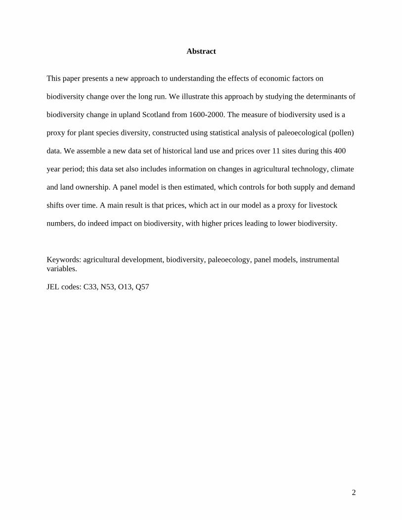
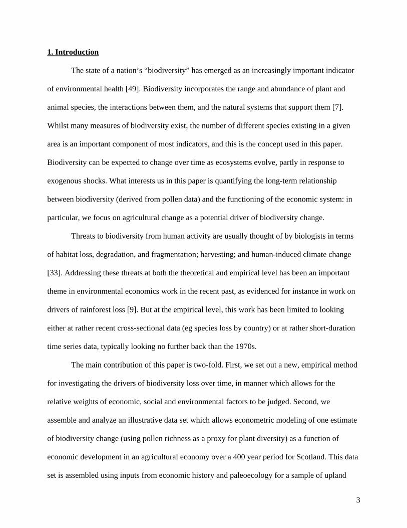
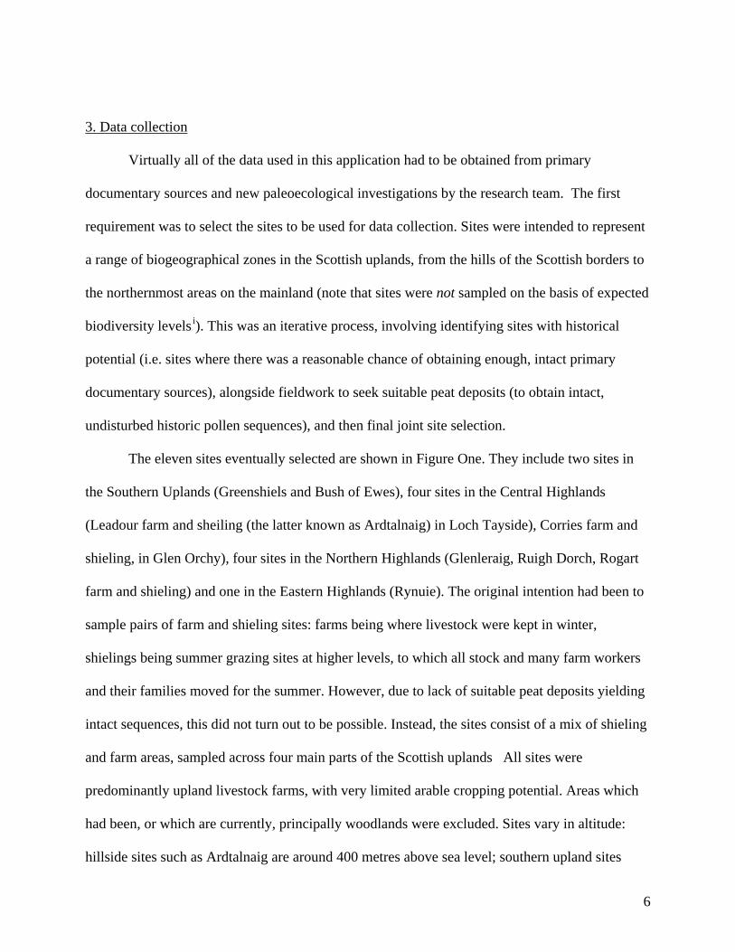
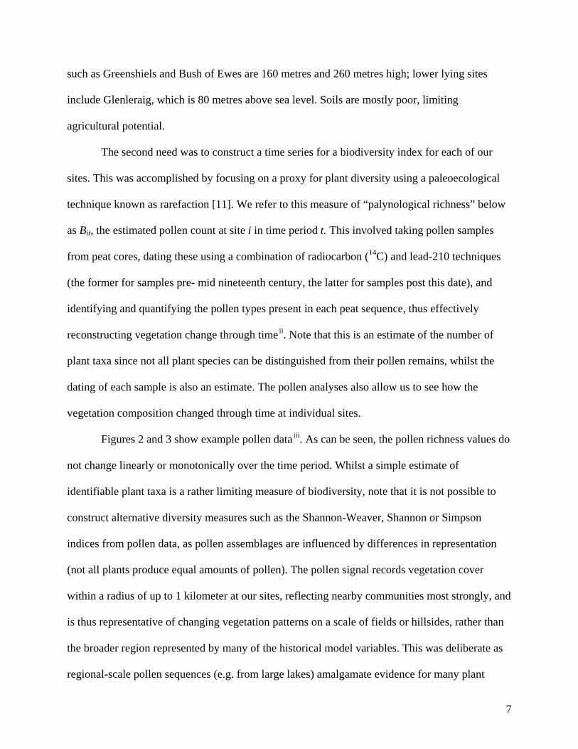
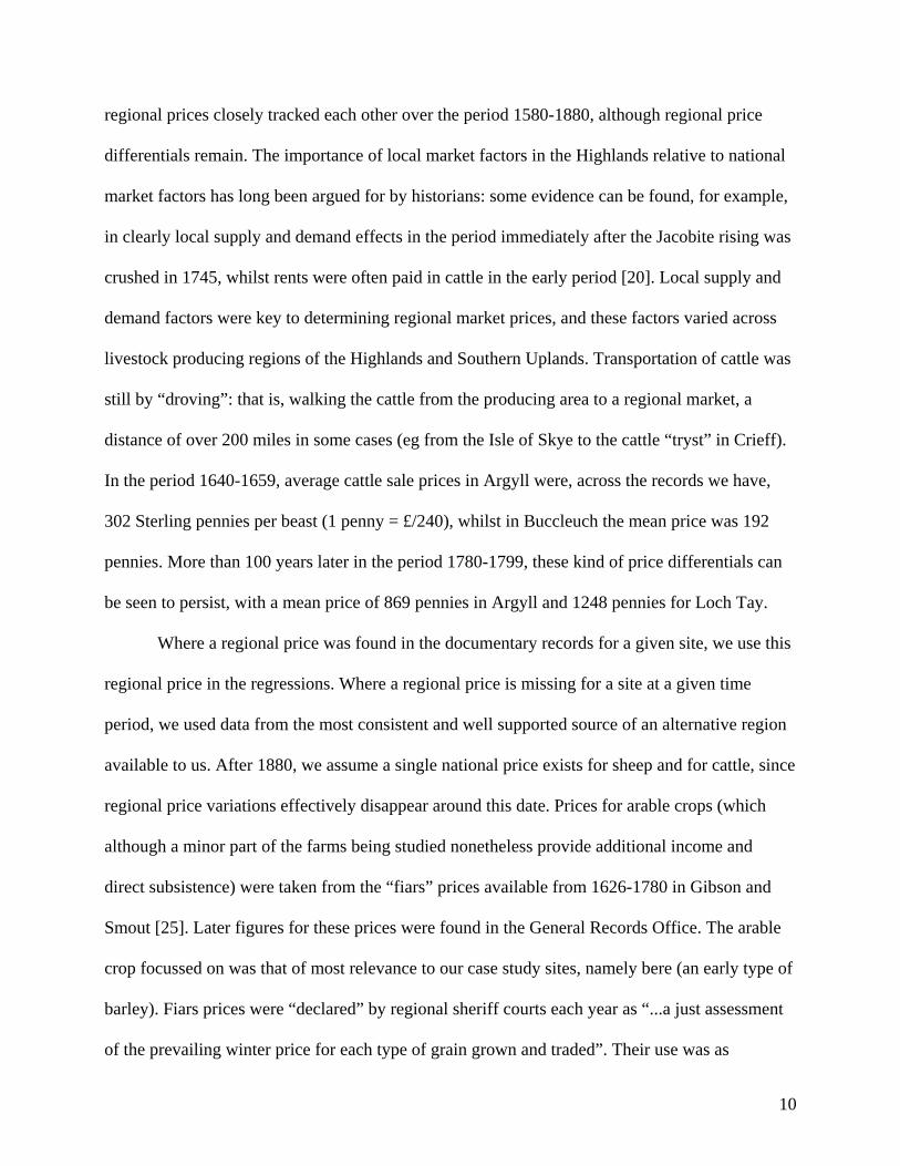
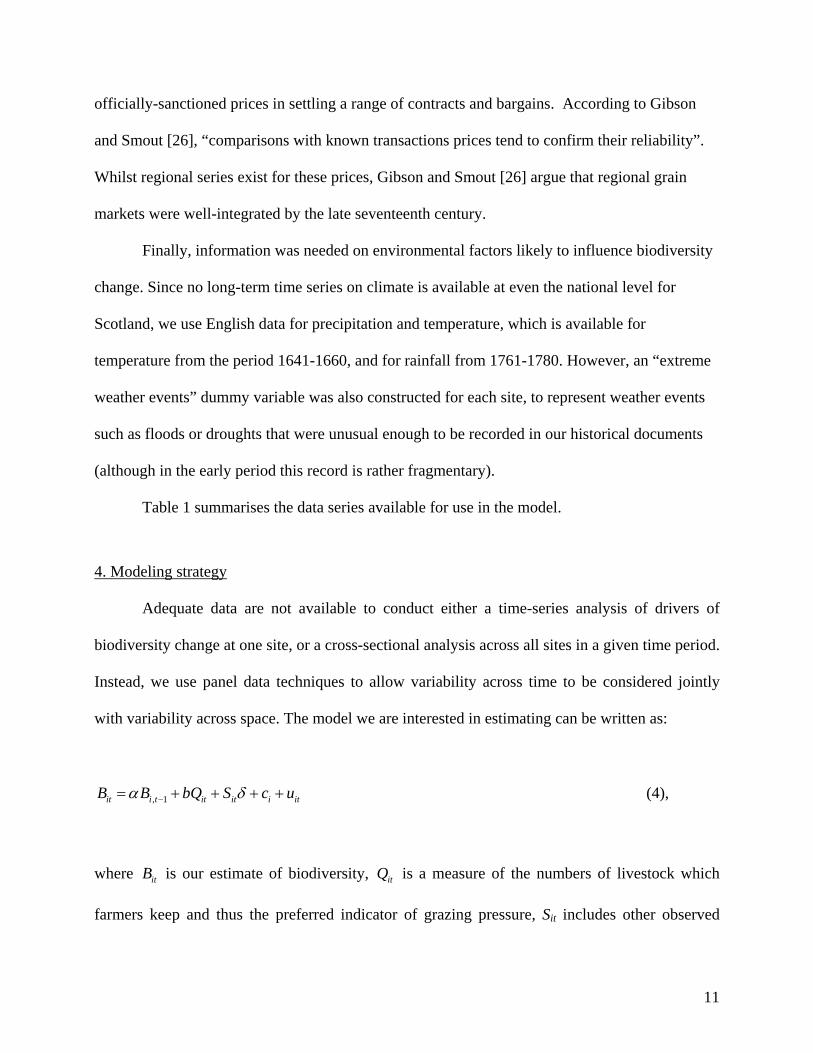
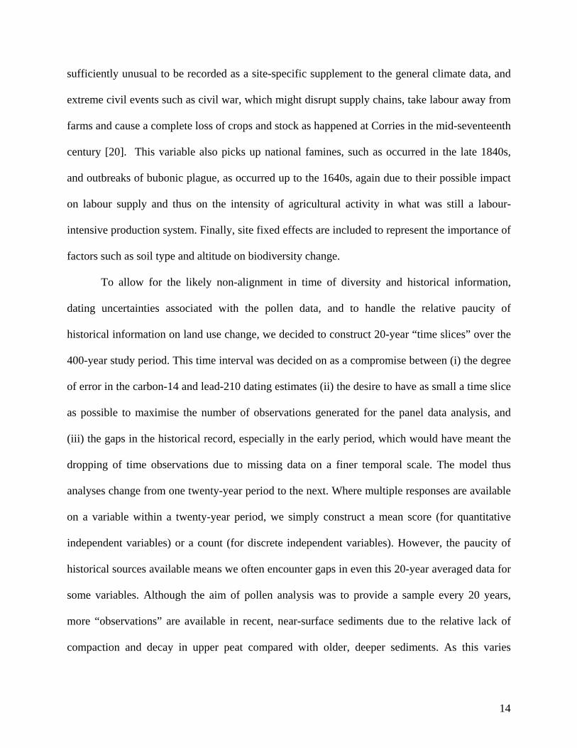
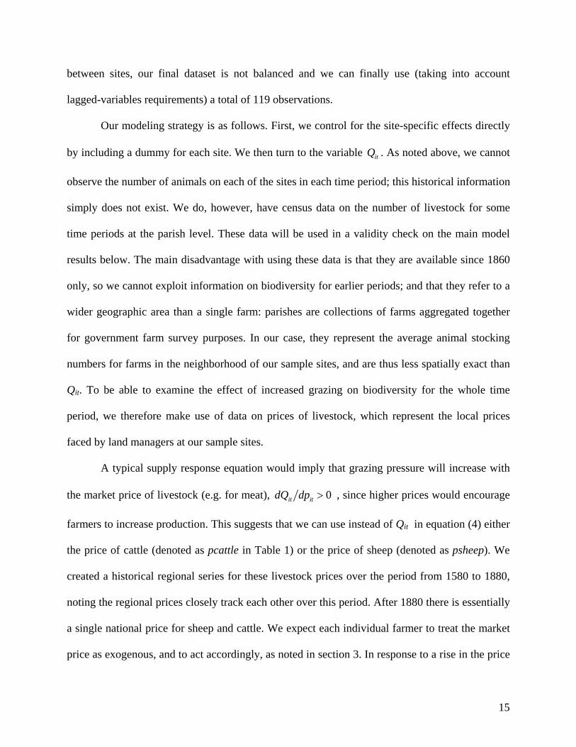
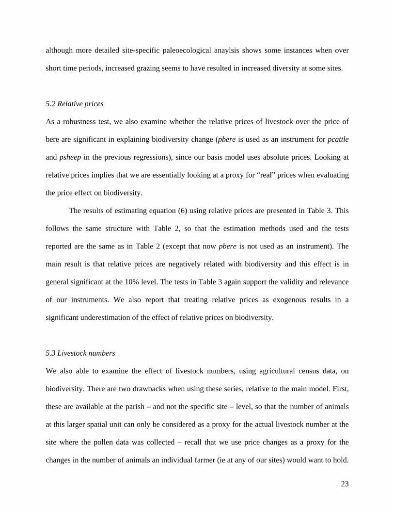
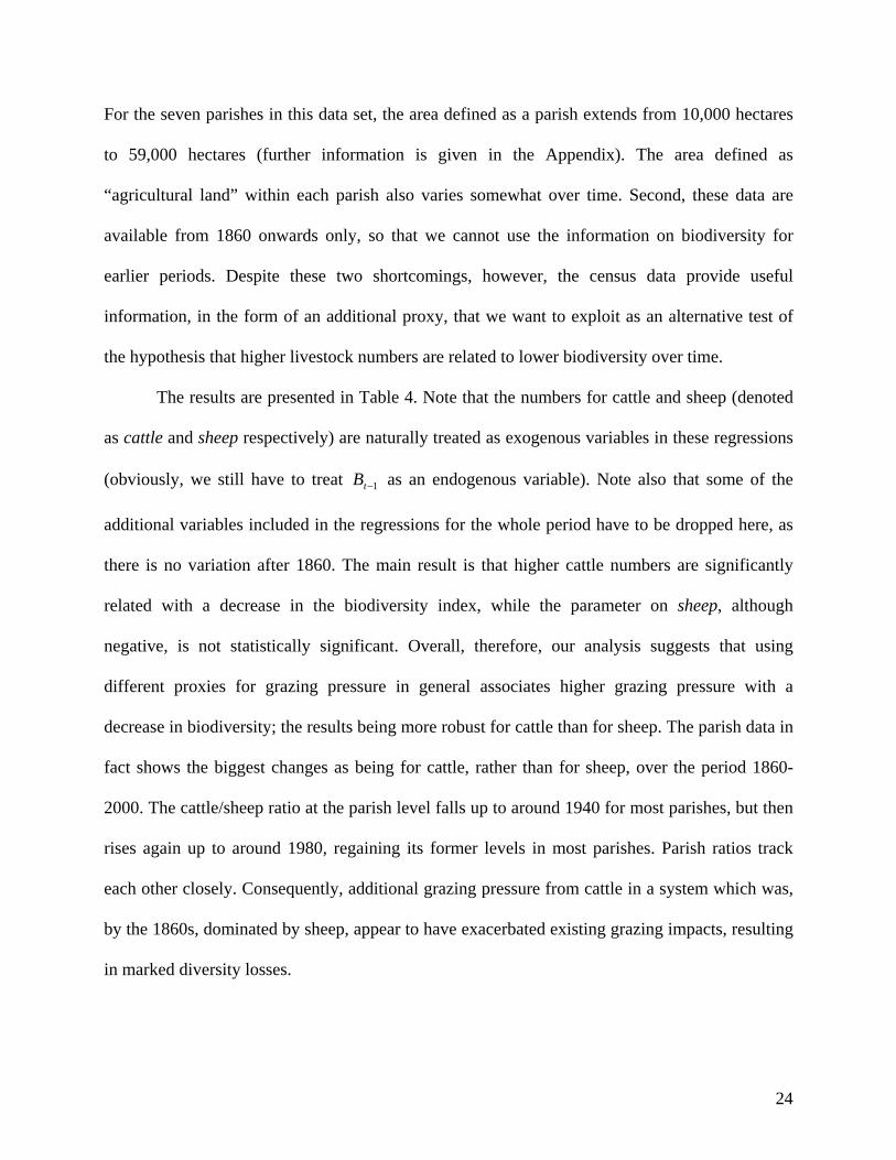
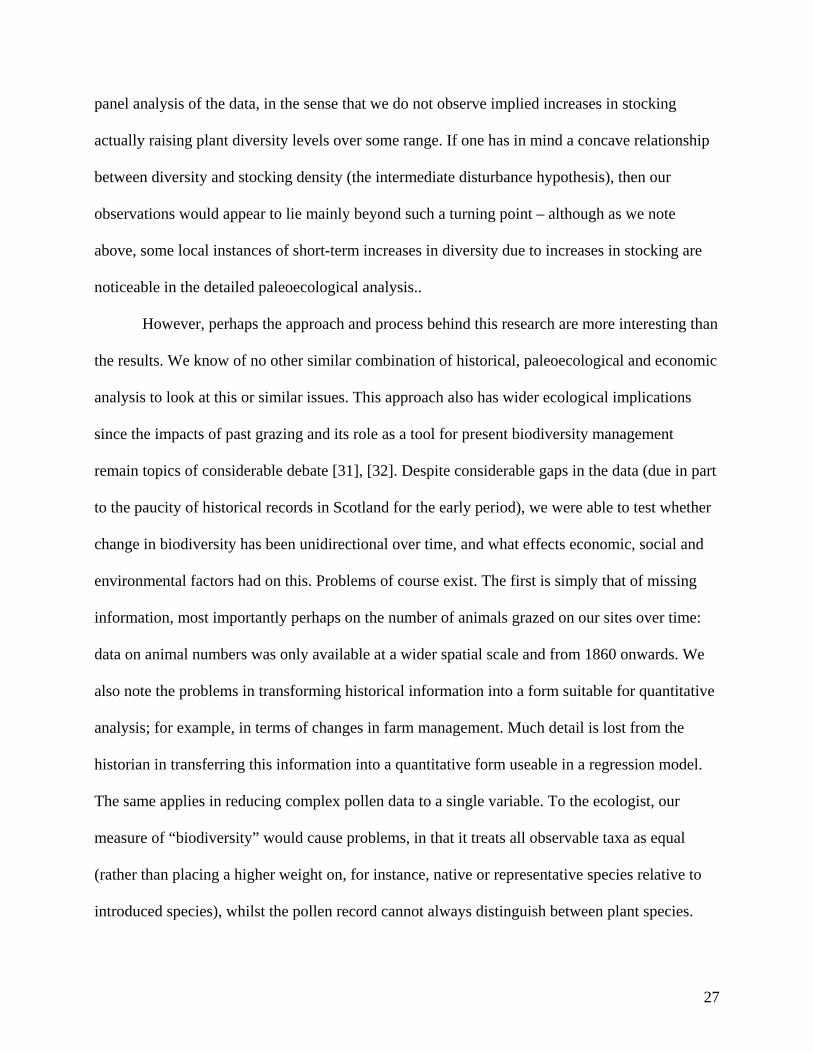
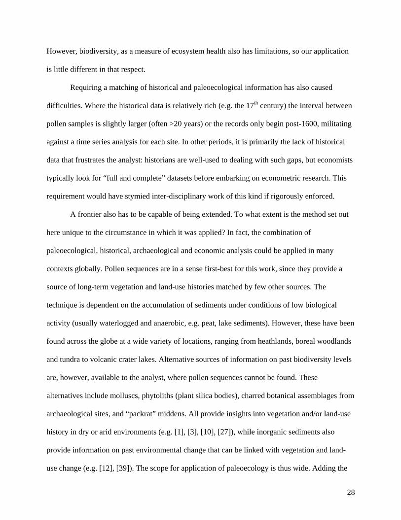
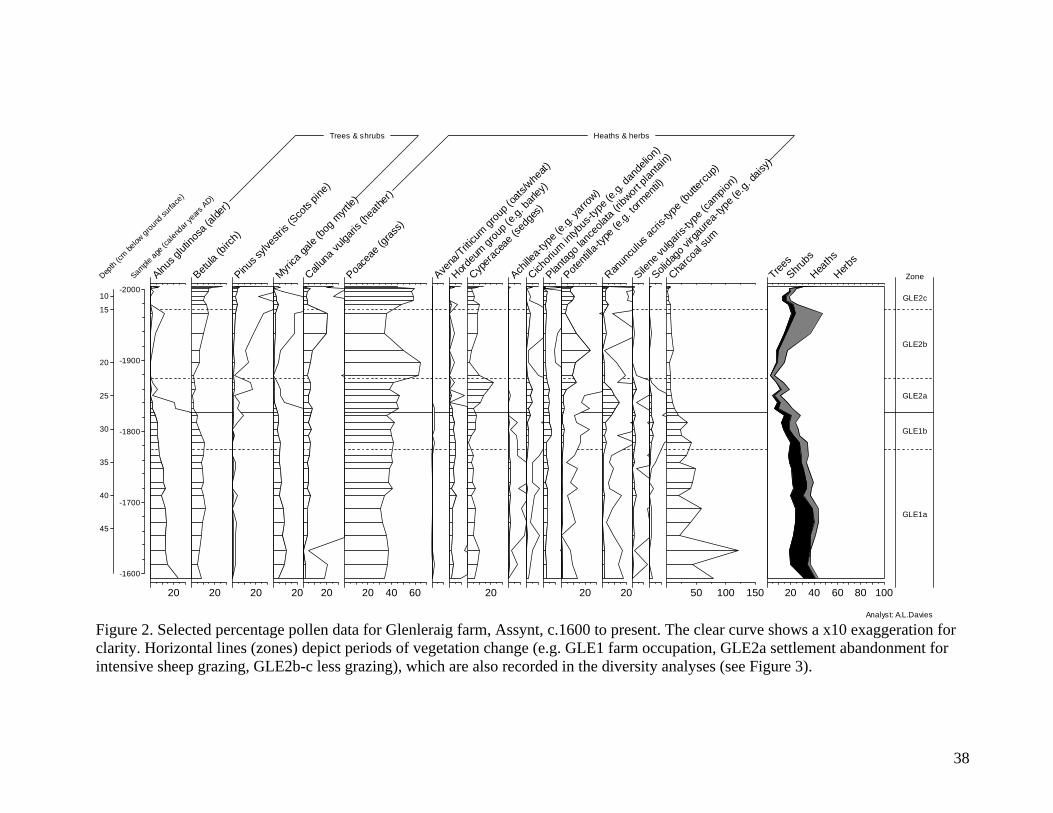
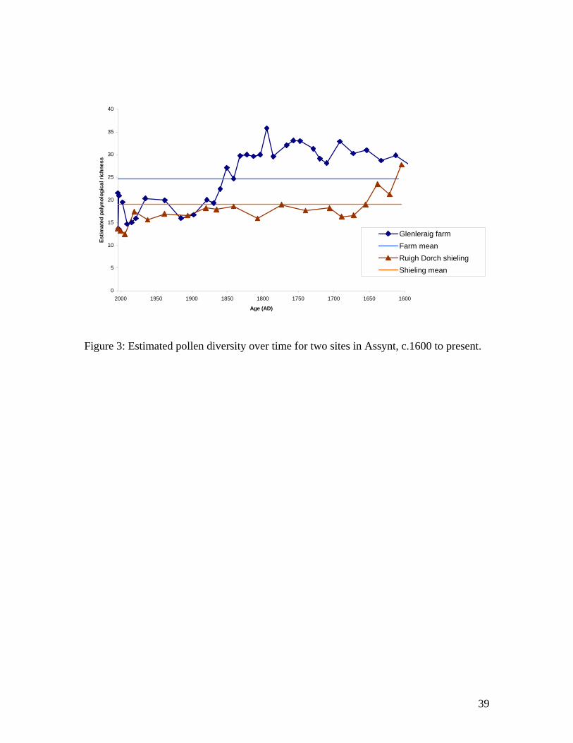
Figures 2 and 3 show example pollen data2F
iii. As can be seen, the pollen richness values do
not change linearly or monotonically over the time period. Whilst a simple estimate of
identifiable plant taxa is a rather limiting measure of biodiversity, note that it is not possible to
construct alternative diversity measures such as the Shannon-Weaver, Shannon or Simpson
indices from pollen data, as pollen assemblages are influenced by differences in representation
(not all plants produce equal amounts of pollen). The pollen signal records vegetation cover
within a radius of up to 1 kilometer at our sites, reflecting nearby communities most strongly, and
is thus representative of changing vegetation patterns on a scale of fields or hillsides, rather than
the broader region represented by many of the historical model variables. This was deliberate as
regional-scale pollen sequences (e.g. from large lakes) amalgamate evidence for many plant
8
communities and land-uses, thus introducing many uncertainties to the ecological interpretation
of both vegetation patterning and the drivers of change. Furthermore, our case studies include
numerous pairs of sites, which reflect spatial and temporal patterns within single farm
management units.
The third need was to construct a historical and cross-sectional database of agricultural
land management. Cattle and sheep grazing was the dominant agricultural land use at the sites we
investigated over the period in question, and we expect impacts on biodiversity to depend on how
intensively land was managed - particularly in terms of stocking rates - and what technology was
available and utilized (e.g. new breeds of sheep which exert different grazing pressure than older
breeds). Few alternative land uses than cattle or sheep production are recorded for our sites:
management decisions thus appear to be mainly concerned with how many cattle or sheep to
stock at any point in time. A contemporary study of agricultural impacts on upland plant diversity
would focus on grazing density, measured in livestock units per hectare (ha). Unfortunately, the
records of livestock numbers and the area grazed on individual farms are very patchy, and official
data was only collected on this from the 1860s onwards, and then only at a higher level of spatial
aggregation, known as the parish. Individual farm estate records typically do not record either the
area being grazed or the total number of livestock at individual sites. We thus cannot use a
modern grazing intensity measure. Instead, we reconstruct a time series of prices for livestock
and crops by region, since we can expect that higher prices of livestock (for meat) and other
products (e.g. wool), ceteris paribus, would motivate farmers to increase their herds as a normal
supply response. However, we are able to represent technological change directly, by creating
count variables for tallying recorded instances of new breeds or new agricultural techniques such
as liming, or the introduction of fodder crops at each of our sites (for a perspective on the overall
effects of technological change in agriculture during this period – albeit for English data – see
9
[14])3F
iv. Distinct changes in farm management, such as enclosure, are also recorded, whilst we are
also able to record the degree of utilization of each site through a typical farming year, from
abandonment to summer-only use to year-round cultivation.
The historical data was collected, firstly, from the estate papers (archives of material
relating to the landholdings of particular noble families and encompassing a wide range of
material generated by, most usually, the owners, their estate officials and lawyers, and, less
frequently, their tenant farmers) relating to each site, i.e. Scott of Buccleuch (Bush of Ewes and
Greenshiels study sites), Campbells of Glenorchy/Breadalbane (Leadour, Corries), Sutherland
(Glenleraig, Rogart), Grant of Freuchy (Rynuie). These are mostly to be found in the National
Archives of Scotland in Edinburgh, although some of the Sutherland papers are still held in situ.
As well as searching for evidence specifically for each site and of the kind of quantitative and
qualitative detail necessary for the model (e.g. animal breeds, prices, ownership patterns, changes
in land management), we also collected more general material, both spatially (i.e. covering
neighboring farms to act as a comparison, corroboration, or fill data gaps) and socially (i.e.
material of a more general nature to illuminate the wider estate/regional context within which our
sites fitted). Finally, because of the lack of price data at a site-specific level, neighbouring estate
papers were also consulted to provide a credible dataset at the regional market level. A timeline
of significant external events (e.g. national or significant regional famine, major periods of
warfare) was also constructed from secondary sources to act as a wider context for site specific
activity.
Prices for livestock (sheep and cattle) were taken from estate papers, as noted above, for
the early period, and from secondary sources for later periods. In the early period, these prices
often relate to local livestock auctions, and price series were assembled for each region in our
analysis. Despite these regional price series being rather patchy and incomplete, they show that
10
regional prices closely tracked each other over the period 1580-1880, although regional price
differentials remain. The importance of local market factors in the Highlands relative to national
market factors has long been argued for by historians: some evidence can be found, for example,
in clearly local supply and demand effects in the period immediately after the Jacobite rising was
crushed in 1745, whilst rents were often paid in cattle in the early period [20]. Local supply and
demand factors were key to determining regional market prices, and these factors varied across
livestock producing regions of the Highlands and Southern Uplands. Transportation of cattle was
still by “droving”: that is, walking the cattle from the producing area to a regional market, a
distance of over 200 miles in some cases (eg from the Isle of Skye to the cattle “tryst” in Crieff).
In the period 1640-1659, average cattle sale prices in Argyll were, across the records we have,
302 Sterling pennies per beast (1 penny = £/240), whilst in Buccleuch the mean price was 192
pennies. More than 100 years later in the period 1780-1799, these kind of price differentials can
be seen to persist, with a mean price of 869 pennies in Argyll and 1248 pennies for Loch Tay.
Where a regional price was found in the documentary records for a given site, we use this
regional price in the regressions. Where a regional price is missing for a site at a given time
period, we used data from the most consistent and well supported source of an alternative region
available to us. After 1880, we assume a single national price exists for sheep and for cattle, since
regional price variations effectively disappear around this date. Prices for arable crops (which
although a minor part of the farms being studied nonetheless provide additional income and
direct subsistence) were taken from the “fiars” prices available from 1626-1780 in Gibson and
Smout [25]. Later figures for these prices were found in the General Records Office. The arable
crop focussed on was that of most relevance to our case study sites, namely bere (an early type of
barley). Fiars prices were “declared” by regional sheriff courts each year as “...a just assessment
of the prevailing winter price for each type of grain grown and traded”. Their use was as
11
officially-sanctioned prices in settling a range of contracts and bargains. According to Gibson
and Smout [26], “comparisons with known transactions prices tend to confirm their reliability”.
Whilst regional series exist for these prices, Gibson and Smout [26] argue that regional grain
markets were well-integrated by the late seventeenth century.
Finally, information was needed on environmental factors likely to influence biodiversity
change. Since no long-term time series on climate is available at even the national level for
Scotland, we use English data for precipitation and temperature, which is available for
temperature from the period 1641-1660, and for rainfall from 1761-1780. However, an “extreme
weather events” dummy variable was also constructed for each site, to represent weather events
such as floods or droughts that were unusual enough to be recorded in our historical documents
(although in the early period this record is rather fragmentary).
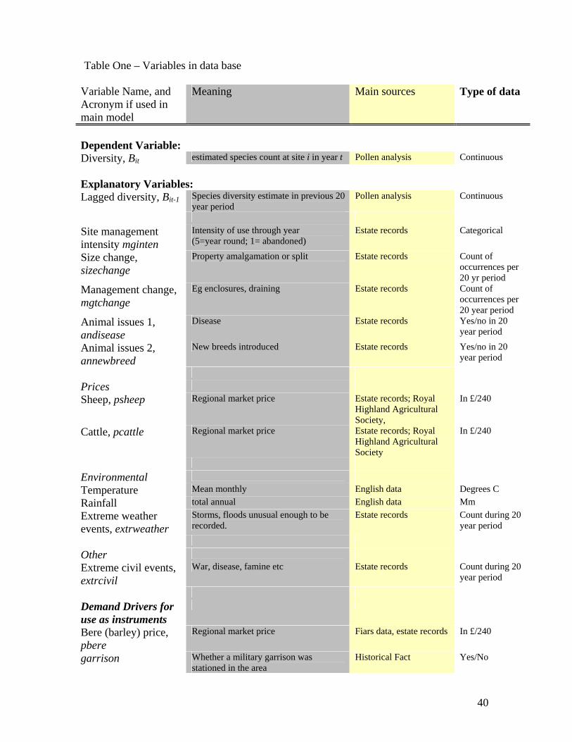
Table 1 summarises the data series available for use in the model.
4. Modeling strategy
Adequate data are not available to conduct either a time-series analysis of drivers of
biodiversity change at one site, or a cross-sectional analysis across all sites in a given time period.
Instead, we use panel data techniques to allow variability across time to be considered jointly
with variability across space. The model we are interested in estimating can be written as:
, 1it i t it it i itB B bQ S c uα δ−= + + + + (4),
where itB is our estimate of biodiversity, itQ is a measure of the numbers of livestock which
farmers keep and thus the preferred indicator of grazing pressure, Sit includes other observed
12
variables that are also thought to affect biodiversity, ic are site-specific (fixed) effects relating to
biodiversity levels (such as soil type and elevation), itu is the idiosyncratic error term and
, ,bα δ are parameters to be estimated. 4F
v Our null hypothesis, based on the ecological work cited
above, is that increases in Q will be associated with declines in B. We will also test whether a
quadratic relationship exists between Q and B, namely whether the data shows that increased
grazing pressure increases plant diversity up to some turning point (threshold), and then reduces
it.
Our estimate of biodiversity is also, however, state dependent. Past vegetation
composition and land-use influence current ecology, but the rates at which plants respond to
change may differ between species. The ecological argument is thus in favor of including the past
pollen diversity estimate as a determinant of the current diversity at a site. We therefore include a
lagged term for diversity, , 1i tB − as a predictor of itB . We expect higher values for , 1i tB − to result in
higher values of itB . However, our main interest here lies on the effect of economic variables on
biodiversity and primarily on the effect of the variable itQ on biodiversity. As we noted, we
cannot directly observe itQ . We would expect, as per Section 1, that higher livestock densities are
in general associated with lower levels of plant diversity, although we also allow for other
influences which might have caused changes on or in the ground. For instance, we include in Sit
management variables, such as sizechange, mgtchange and mgtinten. The first of these represents
whether farm amalgamations occurred in a time period. We know historically that such
amalgamations are sometimes linked to changes in management, particularly in the Improvement
period when many landowners deliberately encouraged, or acquiesced in, the transformation of
the agricultural landscape from multiple-tenanted “fermetouns” to single-tenant farms as part of a
wider revolution in agricultural practices and organisation [19]. Mgtchange is a count variable
13
which represents changes such as enclosure and large-scale draining, again associated with the
multiple major changes that formed part of the Improvement revolution, but also allowing us to
trace the potential effects of small-scale change in other periods. Enclosure is only noted at three
of our sites: Abernethy in 1763, Rogart between 1781-1800 and Corries in 1841. Enclosure has
been argued to have been responsible for a major increase in Scottish agricultural productivity
(eg [18]) but this has been questioned by others, who pinpoint the late 17th and early 19th
centuries as being more associated with major increases in output, with output stagnating or even
falling during the main period of enclosure (eg see [22], [48]; and, for a similar viewpoint in an
English context, [2]). Mgtinten represents how much of the year the site was actively managed
for agriculture, from abandonment, to summer-only use as a sheiling, to year-round use for
grazing. This is an important aspect of the overall history of a site to be taken into account, since
almost all experienced such a change at least once during the time period studied (for example,
Leadour was abandoned as a farm unit in the 1880s, after being grazed continually since 1580 by
the tenant: Rogart changed from summer only use up to 1780 to year-round use, and then was
abandoned but still occasionally grazed from 1820). A small literature exists on the effects of site
abandonment which led us to wish to examine this factor in the present study [41], [21], whilst
the variable also allowed for control over the changing seasonal management of a site noted
above.
Finally we included in Sit some historical, technological and climatological variables that
the interdisciplinary team deemed likely to affect biodiversity. These are andisease, annewbread,
extrweather and extrcivil. These represent major outbreaks of animal disease (associated with
falling stocking densities), the introduction of new breeds (the new type of Cheviot sheep
introduced at various times to our sites were much bigger than the native breeds and might be
expected, therefore, per head, to have higher grazing demands), extreme weather events that were
14
sufficiently unusual to be recorded as a site-specific supplement to the general climate data, and
extreme civil events such as civil war, which might disrupt supply chains, take labour away from
farms and cause a complete loss of crops and stock as happened at Corries in the mid-seventeenth
century [20]. This variable also picks up national famines, such as occurred in the late 1840s,
and outbreaks of bubonic plague, as occurred up to the 1640s, again due to their possible impact
on labour supply and thus on the intensity of agricultural activity in what was still a labour-
intensive production system. Finally, site fixed effects are included to represent the importance of
factors such as soil type and altitude on biodiversity change.
To allow for the likely non-alignment in time of diversity and historical information,
dating uncertainties associated with the pollen data, and to handle the relative paucity of
historical information on land use change, we decided to construct 20-year “time slices” over the
400-year study period. This time interval was decided on as a compromise between (i) the degree
of error in the carbon-14 and lead-210 dating estimates (ii) the desire to have as small a time slice
as possible to maximise the number of observations generated for the panel data analysis, and
(iii) the gaps in the historical record, especially in the early period, which would have meant the
dropping of time observations due to missing data on a finer temporal scale. The model thus
analyses change from one twenty-year period to the next. Where multiple responses are available
on a variable within a twenty-year period, we simply construct a mean score (for quantitative
independent variables) or a count (for discrete independent variables). However, the paucity of
historical sources available means we often encounter gaps in even this 20-year averaged data for
some variables. Although the aim of pollen analysis was to provide a sample every 20 years,
more “observations” are available in recent, near-surface sediments due to the relative lack of
compaction and decay in upper peat compared with older, deeper sediments. As this varies
15
between sites, our final dataset is not balanced and we can finally use (taking into account
lagged-variables requirements) a total of 119 observations.
Our modeling strategy is as follows. First, we control for the site-specific effects directly
by including a dummy for each site. We then turn to the variable itQ . As noted above, we cannot
observe the number of animals on each of the sites in each time period; this historical information
simply does not exist. We do, however, have census data on the number of livestock for some
time periods at the parish level. These data will be used in a validity check on the main model
results below. The main disadvantage with using these data is that they are available since 1860
only, so we cannot exploit information on biodiversity for earlier periods; and that they refer to a
wider geographic area than a single farm: parishes are collections of farms aggregated together
for government farm survey purposes. In our case, they represent the average animal stocking
numbers for farms in the neighborhood of our sample sites, and are thus less spatially exact than
Qit. To be able to examine the effect of increased grazing on biodiversity for the whole time
period, we therefore make use of data on prices of livestock, which represent the local prices
faced by land managers at our sample sites.
A typical supply response equation would imply that grazing pressure will increase with
the market price of livestock (e.g. for meat), 0it itdQ dp > , since higher prices would encourage
farmers to increase production. This suggests that we can use instead of Qit in equation (4) either
the price of cattle (denoted as pcattle in Table 1) or the price of sheep (denoted as psheep). We
created a historical regional series for these livestock prices over the period from 1580 to 1880,
noting the regional prices closely track each other over this period. After 1880 there is essentially
a single national price for sheep and cattle. We expect each individual farmer to treat the market
price as exogenous, and to act accordingly, as noted in section 3. In response to a rise in the price
16
of livestock the farmer will want to sell more livestock, and thus will increase the existing herd
size on the farm. The result of this supply response, according to (4), should ceteris paribus be a
fall in Bit. However, since the observed prices are endogenous, as equilibrium prices are jointly
determined with quantity, this effect is uncertain in our analysis. The main concern with
substituting our observed livestock prices pcattle and psheep for itQ in (4) is therefore that prices
are endogenous in this regression, as their effect is not immediately identified as a demand or a
supply effect.
If we could assume the existence of a supply equation,
it t it itQ P S eη θ= + + (5)
then an increase in prices would result in an increase in the number of animals per ha and hence a
decrease in the number of species (a fall in itB ). This requires that equation (5) is identified as a
supply equation; in this case, we would expect η to be positive in (5). However, the equilibrium
prices that we observe historically are most likely an endogenous outcome, determined jointly
with quantity. In this case, the effect of prices in (5), and hence in (4) may be affected by reverse
causality, and therefore is not identified. In other words, we do not know if, when estimating
equation (5), we estimate a supply or a demand function. A demand function would imply a
negative η . Hence, endogeneity of prices in (5) implies that we cannot ex ante sign η . If we do
not indentify (5) as a supply equation, we should expect a downward bias in our estimate in η .
This then implies that the effect of prices in (4) is not indentified.
To make this clear, substitute (5) in (4) to get (note that the supply shifters in (5) are
essentially the variables already included as Sit in (4)):
17
( ), 1
, 1
( ) ,
, ,
it i t t it i it it
it i t t it i it
it it it
B B b P S b c u be orB B P S c vwhere
b b v u be
α η δ θ
α β γ
β η γ δ θ
−
−
= + + + + + +
= + + + +
= = + = +
(6)
Therefore, , ,α β γ are the parameters we can estimate in (6). If itP is correlated with ite in
(5), then itP will also be correlated with itv in (6). This implies that if the estimation of (6) does
not take into account this type of endogeneity of prices, the downward (simultaneity) bias of η in
(5) will result in underestimating β in (6), as it will be biased towards zero.
Our approach to identify the effect of itP in (6) is essentially the method used to identify
itP in a supply equation like (5). That is, we use demand shifters that are correlated with prices,
but uncorrelated with ite (and hence with itv ), as instruments in IV methods to estimate (6). In
this way, since itP is identified in (5), we expectη to be positive and thus a negative β will imply
a negativeb . As demand shifters we use the variables: pbere, garrison, union, popenglish and
refrigeration. All these variables are expected to have affected demand for meat in Scotland. The
price of bere (barley) pbere is used as the price of a substitute good in consumption (none of our
sites engaged in significant grain production, due to their locations). When the price of bere
increases, consumers would increase their demand for substitutes, including meat, and hence the
demand for cattle and sheep would increase. Regarding garrison, it was a feature of the
Highlands from the mid-seventeenth century onwards that particular areas had a military garrison
installed for considerable periods of time, even beyond periods of civil unrest and actual warfare.
This acted as a new and potentially lucrative market for both meat and grain, as well as bringing
18
highland cattle owners into contact with those familiar with the wider English market during the
Cromwellian occupation (1650-60) [37]. Our sites were not likely to be equally affected by this
aspect.
The union variable refers to the impact of the act of incorporating union between the
parliaments of England and Scotland, creating the single parliament of Great Britain. The
practical aspects of this involved the relaxing of trade barriers between England and Scotland
which, prior to then, had operated as two separate countries (as, indeed, they were) with their
own restrictive tariffs, mostly on the English side. This removal of trade barriers with England
gave additional impetus to the growing market in black cattle particularly, which had begun in
the previous century [40]. The variable popenglish is included given that we would expect that
increased population in England represents increased demand from consumers in England for
Scottish livestock exports. Finally, refrigeration is expected to have had a negative effect on the
demand for Scottish-produced meat, as the advent of refrigerated transport in the 1890s meant
that consumers could substitute imported meat from the New World for Scottish meat. Overall,
this set of variables were derived from an overview of the historical literature to enable us to
ascertain the key issues most likely to have had an effect on demand for livestock production in
Scotland. These variables can be thought of as unrelated with either ite or itu , conditioning on the
right hand side variables in equations (5) and (6) and can thus be used together with the variables
in itS as instruments for the prices. In any case, the validity of the instruments will be tested by
over-identification tests. We will also examine the effects of treating prices as exogenous in (6).
The final issue we deal with is the presence of the lagged endogenous variable as a
regressor. This implies that (6) will not satisfy the strict exogeneity assumption needed for the
fixed effects estimator to be consistent, as itv will be correlated with future realizations of , 1i tB − .
19
In such dynamic models, the usual approach is to exploit sequential moment restrictions, i.e. the
fact that the error term is correlated with leads but not with lags of , 1i tB − , and use the latter as
instruments in IV methods. As the main interest here lies in consistently estimating (primarily) β
and (also) γ , we deal with potential biases introduced by , 1i tB − , by using , 2i tB − , along with the
demand shifters and the variables in itS to instrument , 1i tB − (see e.g. [43], for panel data models
without the strict exogeneity assumption).
5. Results
We start by presenting the basic results obtained for the whole period, using prices for livestock
to estimate equation (6) as described above, within a fixed effects IV panel model. We then
discuss the robustness of these basic results by using relative prices, testing for breaks in price
endogeneity, and also present results obtained by using parish census livestock data for the period
starting from 1860.
5.1 Livestock prices – the main model.
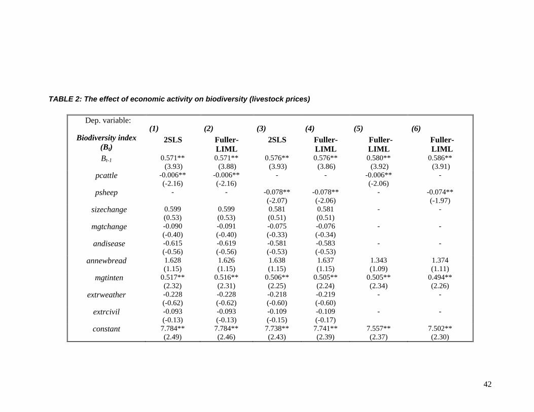
Results from the panel model are presented in Table 2. All regressions include a dummy for each
site. The first two columns present results using pcattle for itP in (6), and the following two
columns we use psheep for itP . As the two prices are highly correlated (the correlation coefficient
is 0.99) it makes little sense to include them together in the regression. The variables , 1i tB − , pcattle
and psheep are treated as endogenous and the excluded instruments in these regressions are , 2i tB − ,
popenglish, war, union, refrigeration and pbere.5F
vi Columns (1) and (3) presents 2SLS results
while columns (2) and (4) report results obtained by Fuller’s [24] modified LIML, with a = 1, as
20
it has been found in simulation studies to be more robust to potentially weak instruments (the
potential biases due to weak instruments are much smaller with LIML, see [6] and [43].
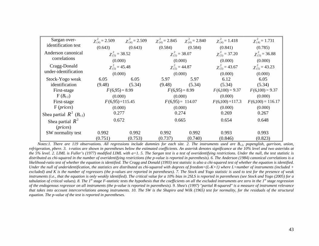
Before discussing the results, we note that the model does well with respect to the
diagnostics for the validity and relevance of the instruments. In particular, we first see that the
Sargan over-identifying tests clearly support the null that the instruments are uncorrelated with
the structural error term. In addition, the Anderson [4] canonical correlations and the Cragg and
Donald [16] tests reject the null of under-identification. To further examine instrument relevance,
we report the first stage F-statistics (of the test that the joint effect of the excluded instruments on
the endogenous variable is zero in the first stage regression) and Shea’s [36] first stage “partial
R-squared”. Both present strong evidence of high correlation of the instruments with the
endogenous variables (especially with prices). The Stock and Yogo [43] tests for weak
instruments suggest that the first stage correlations may introduce biases in the 2SLS regressions
but not in LIML regressions and thus favour Fuller’s LIML estimator. In any case, we do not find
important differences between the 2SLS and LIML estimates. Finally, Shapiro and Wilk [35]
tests for normality suggest that the residuals from the structural equations are in all regressions
normally distributed.
The results show that higher prices for both sheep and cattle imply lower levels of
biodiversity over time and across sites. The implication is that the rise in the price in livestock
markets for “meat on the hoof” means that the farmer will want to sell more livestock, and thus
will want to increase the existing herd size, which in turn results in a loss in plant species
diversity. This response seems to “confirm” modern ecological thinking about the likely effects
of overgrazing on fragile upland ecosystems. It is interesting to note the implication that
increased sheep grazing (as captured by increases in the price of sheep) has been much worse for
biodiversity than increased cattle grazing (as captured by increases in the price of cattle) –

21
although recall that these parameters refer to increases in prices, not increases in animal numbers
which are only inferred – we do not know how elastic the supply response was at individual sites,
or on average. The only other variable that emerges as significant is the degree to which sites are
managed year-round; results show that abandonment of sites reduces biodiversity. Neither
technological innovations nor extreme weather events seem to matter to our estimate of
biodiversity. Finally, in accord with expectations, it can be seen that higher plant species numbers
in preceding periods are associated with higher species numbers in subsequent periods – there is a
biological inheritance effect present in the data.
Since most of the variables in itS are not significant, we repeat the regressions in columns
(2) and (4) by keeping only annewbreed and mgtinten to check whether the estimates for the
main variables of interest are affected by the inclusion of irrelevant variables (the former variable
was retained since there has been considerable interest in the effects of new breeds on
biodiversity). The new results are reported in columns (5) and (6). As may be seen, this produced
no major changes to the results noted above.
We also have examined what happens when prices are treated as exogenous when
estimating equation (6). It turns out that the biases introduced by the correlation of prices with the
error term (reverse causality) are of the order of 100%, as both coefficients have half of the
values reported in Table 2 (and are not statistically significant), while the estimates for the other
coefficients do not differ greatly. As a further exercise to investigate the effect of endogeneity
bias in our estimates by treating prices as exogenous, we split the sample into pre- and post- 1880
(by 1880, as discussed above, our working assumption is that markets were well integrated to
assume more or less a common price). We would expect endogeneity bias from OLS estimation
to be larger in the pre 1880 sub-sample, as local prices would react stronger to local market
22
forces; on the contrary, national prices should be less influenced by shocks in local markets and
mainly react to national demand and supply. Indeed, when we re-estimate our model for the two
sub-samples and look at the size of the estimated coefficients obtained from 2SLS and OLS
estimation, we find that endogeneity bias is clearly high in the pre-1880 period – again, about
100% for the price of cattle and 80% for the price of sheep. In contrast, for the post-1880 period,
the 2SLS and OLS estimated coefficients are very close for the price of cattle suggesting no
endogeneity in prices, although there is still a difference for the price of sheep (all estimated
coefficients, in both sub-samples, using both 2SLS and OLS, are negative). As a remark of
caution, we note that we have to treat these results with caution, as they are based on small
samples (the degrees of freedom drop to about 55 for the pre-1880 sample and 30 for post-1880),
so that estimates are not precise and hence the estimated coefficients are not statistically
significant. Nevertheless, they are supportive of the argument that regional prices are likely to be
endogenous in our regressions prior to 1880, and that not accounting for this will bias our
estimates.6F
vii
In addition, we report that we have examined whether including some additional
climatological variables affects our results. Variables describing changes in mean annual
temperature and rainfall are not significant when they are entered into our regressions and they do
not affect the results described above. However, since no long term climatic time series exist for
Scotland, we have to use English data for these variables: this may contribute to the lack of
statistical significance. Finally, a quadratic relationship between Q and B was tested for: as noted
above, this would imply that up to some point, increasing grazing pressure actually increases
plant diversity, but that after this turning point or threshold, increased grazing pressure reduces
diversity. However, results show that no such effect is revealed in the data presented here,
23
although more detailed site-specific paleoecological anaylsis shows some instances when over
short time periods, increased grazing seems to have resulted in increased diversity at some sites.
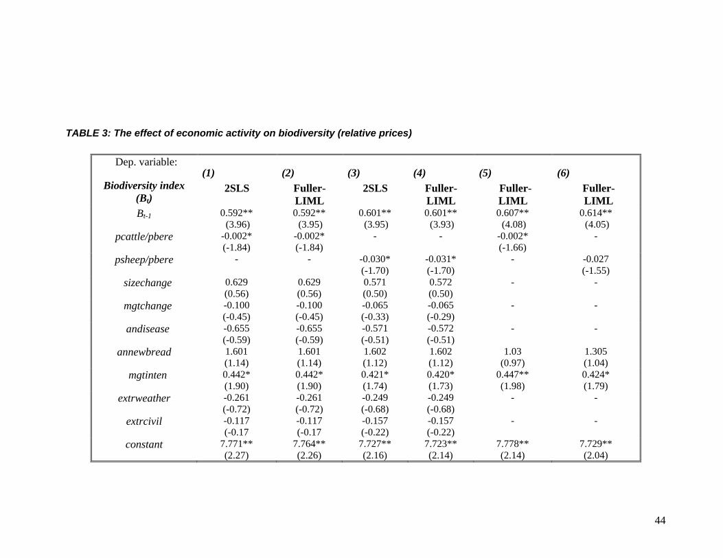
5.2 Relative prices
As a robustness test, we also examine whether the relative prices of livestock over the price of
bere are significant in explaining biodiversity change (pbere is used as an instrument for pcattle
and psheep in the previous regressions), since our basis model uses absolute prices. Looking at
relative prices implies that we are essentially looking at a proxy for “real” prices when evaluating
the price effect on biodiversity.
The results of estimating equation (6) using relative prices are presented in Table 3. This
follows the same structure with Table 2, so that the estimation methods used and the tests
reported are the same as in Table 2 (except that now pbere is not used as an instrument). The
main result is that relative prices are negatively related with biodiversity and this effect is in
general significant at the 10% level. The tests in Table 3 again support the validity and relevance
of our instruments. We also report that treating relative prices as exogenous results in a
significant underestimation of the effect of relative prices on biodiversity.
5.3 Livestock numbers
We also able to examine the effect of livestock numbers, using agricultural census data, on
biodiversity. There are two drawbacks when using these series, relative to the main model. First,
these are available at the parish – and not the specific site – level, so that the number of animals
at this larger spatial unit can only be considered as a proxy for the actual livestock number at the
site where the pollen data was collected – recall that we use price changes as a proxy for the
changes in the number of animals an individual farmer (ie at any of our sites) would want to hold.
24
For the seven parishes in this data set, the area defined as a parish extends from 10,000 hectares
to 59,000 hectares (further information is given in the Appendix). The area defined as
“agricultural land” within each parish also varies somewhat over time. Second, these data are
available from 1860 onwards only, so that we cannot use the information on biodiversity for
earlier periods. Despite these two shortcomings, however, the census data provide useful
information, in the form of an additional proxy, that we want to exploit as an alternative test of
the hypothesis that higher livestock numbers are related to lower biodiversity over time.
The results are presented in Table 4. Note that the numbers for cattle and sheep (denoted
as cattle and sheep respectively) are naturally treated as exogenous variables in these regressions
(obviously, we still have to treat 1−tB as an endogenous variable). Note also that some of the
additional variables included in the regressions for the whole period have to be dropped here, as
there is no variation after 1860. The main result is that higher cattle numbers are significantly
related with a decrease in the biodiversity index, while the parameter on sheep, although
negative, is not statistically significant. Overall, therefore, our analysis suggests that using
different proxies for grazing pressure in general associates higher grazing pressure with a
decrease in biodiversity; the results being more robust for cattle than for sheep. The parish data in
fact shows the biggest changes as being for cattle, rather than for sheep, over the period 1860-
2000. The cattle/sheep ratio at the parish level falls up to around 1940 for most parishes, but then
rises again up to around 1980, regaining its former levels in most parishes. Parish ratios track
each other closely. Consequently, additional grazing pressure from cattle in a system which was,
by the 1860s, dominated by sheep, appear to have exacerbated existing grazing impacts, resulting
in marked diversity losses.
25
In addition, we see that in Table 4 more variables are significant in explaining
biodiversity change over this later period. An increase in the number of size changes in the farm
holding, whether this was an increase in the farm size due to amalgamations, or (much more
rarely in the records) a decrease due to the farm holding being split up, is associated with a fall in
diversity. Discontinuities in management thus appear to be bad for biodiversity in the data. The
introduction of new breeds produces an increase in diversity, whilst the extent to which sites are
utilised year-round also affects diversity, in line with results from the main model, as may be
seen from the parameter estimate for mginten. The number of management changes such as
burning, liming or fencing (mgtchange) also has a significant effect on diversity in the sheep
numbers model. Finally, extreme weather events in this later period seem to be related to plant
diversity changes.
6. Conclusions
This paper is part of a series commissioned by Resources for the Future on “Frontiers in
Environmental Economics”. In what sense is it “on the frontier”? We think in two ways. First, we
present a new methodology for investigating economic influences on biodiversity, which greatly
extends the temporal range over which analysis can be undertaken. This method involves a
combination of paleoecological methods and environmental historical research with economic
reasoning and econometric analysis. Second, we present what we believe to be the first empirical
application of this method to a specific context. Empirically, the paper set out to investigate the
effects of economic, social and environmental factors on biodiversity over a 400-year period. We
constructed a panel of estimates of plant diversity across space and time using pollen analysis,
and assembled a dataset of prices, land use change, technological improvements and changes in
property rights. Panel regression analysis was then used to explore relationships between the
26
diversity estimate and these economic and social drivers. The main conclusions that emerged
were that agricultural prices exerted significant influences on biodiversity over the period 1600-
2000, as did the extent to which sites were farmed year-round. However, no significant effects
were found for climatic variables, or for extreme civil events, or technology change in the main
model estimated over the entire 400 year period. Robustness analysis which relaxed the
assumption of endogenous prices, and used relative rather than absolute prices and actual
livestock numbers where these are available, seems to confirm our main results for the most part.
Our results might thus be seen as confirming the ecological idea that rising grazing
pressures is bad for biodiversity. These findings show that over the long run, human-induced
biodiversity change was significant for these sites. While the analytical methods applied here are
novel, the results support previous documentary and palaeoecological evidence for some
deterioration in the quality or diversity of the UK uplands around 200-300 years ago, particularly
post-1850 [17], [41], [42], [46]. That increases in grazing rates can lead to decreases in
biodiversity in the uplands is well-recognised in contemporary ecological studies [28], [34], [44],
[45]. For example, Fuller and Gough [23] argue that increases in sheep numbers in upland Wales
from the 1970s to the 1990s “almost certainly” caused reductions in habitat quality for ground-
nesting birds such as waders, partly through the effects on plant cover, leading to a decline in bird
numbers. Our findings essentially confirm that this tendency has existed over a much longer time
period.
The present evidence that abandonment had significant effects on diversity also supports
recent historical inferences [21], [41], although we note that what is actually observed in the data
here is that moving from year-round cultivation or grazing, to summer-only use, and then to
abandonment for any stocking level, has a negative effect on diversity: this effect is distinct from
the effect of the level of grazing pressure. No threshold grazing level effect was found using
27
panel analysis of the data, in the sense that we do not observe implied increases in stocking
actually raising plant diversity levels over some range. If one has in mind a concave relationship
between diversity and stocking density (the intermediate disturbance hypothesis), then our
observations would appear to lie mainly beyond such a turning point – although as we note
above, some local instances of short-term increases in diversity due to increases in stocking are
noticeable in the detailed paleoecological analysis..
However, perhaps the approach and process behind this research are more interesting than
the results. We know of no other similar combination of historical, paleoecological and economic
analysis to look at this or similar issues. This approach also has wider ecological implications
since the impacts of past grazing and its role as a tool for present biodiversity management
remain topics of considerable debate [31], [32]. Despite considerable gaps in the data (due in part
to the paucity of historical records in Scotland for the early period), we were able to test whether
change in biodiversity has been unidirectional over time, and what effects economic, social and
environmental factors had on this. Problems of course exist. The first is simply that of missing
information, most importantly perhaps on the number of animals grazed on our sites over time:
data on animal numbers was only available at a wider spatial scale and from 1860 onwards. We
also note the problems in transforming historical information into a form suitable for quantitative
analysis; for example, in terms of changes in farm management. Much detail is lost from the
historian in transferring this information into a quantitative form useable in a regression model.
The same applies in reducing complex pollen data to a single variable. To the ecologist, our
measure of “biodiversity” would cause problems, in that it treats all observable taxa as equal
(rather than placing a higher weight on, for instance, native or representative species relative to
introduced species), whilst the pollen record cannot always distinguish between plant species.
28
However, biodiversity, as a measure of ecosystem health also has limitations, so our application
is little different in that respect.
Requiring a matching of historical and paleoecological information has also caused
difficulties. Where the historical data is relatively rich (e.g. the 17th century) the interval between
pollen samples is slightly larger (often >20 years) or the records only begin post-1600, militating
against a time series analysis for each site. In other periods, it is primarily the lack of historical
data that frustrates the analyst: historians are well-used to dealing with such gaps, but economists
typically look for “full and complete” datasets before embarking on econometric research. This
requirement would have stymied inter-disciplinary work of this kind if rigorously enforced.
A frontier also has to be capable of being extended. To what extent is the method set out
here unique to the circumstance in which it was applied? In fact, the combination of
paleoecological, historical, archaeological and economic analysis could be applied in many
contexts globally. Pollen sequences are in a sense first-best for this work, since they provide a
source of long-term vegetation and land-use histories matched by few other sources. The
technique is dependent on the accumulation of sediments under conditions of low biological
activity (usually waterlogged and anaerobic, e.g. peat, lake sediments). However, these have been
found across the globe at a wide variety of locations, ranging from heathlands, boreal woodlands
and tundra to volcanic crater lakes. Alternative sources of information on past biodiversity levels
are, however, available to the analyst, where pollen sequences cannot be found. These
alternatives include molluscs, phytoliths (plant silica bodies), charred botanical assemblages from
archaeological sites, and “packrat” middens. All provide insights into vegetation and/or land-use
history in dry or arid environments (e.g. [1], [3], [10], [27]), while inorganic sediments also
provide information on past environmental change that can be linked with vegetation and land-
use change (e.g. [12], [39]). The scope for application of paleoecology is thus wide. Adding the
29
economic dimension to paleoecology requires a theoretical view on what human or
environmental influences drive the system under study, and the ability to construct data sets of
those influences that are measurable, such as climate change, prices and technological
innovations. For this, the economist needs to work closely with colleagues in history and
archaeology. But the gains from analysis seem likely to be great in terms of generating new
insights into what drives long-term biodiversity change.
30
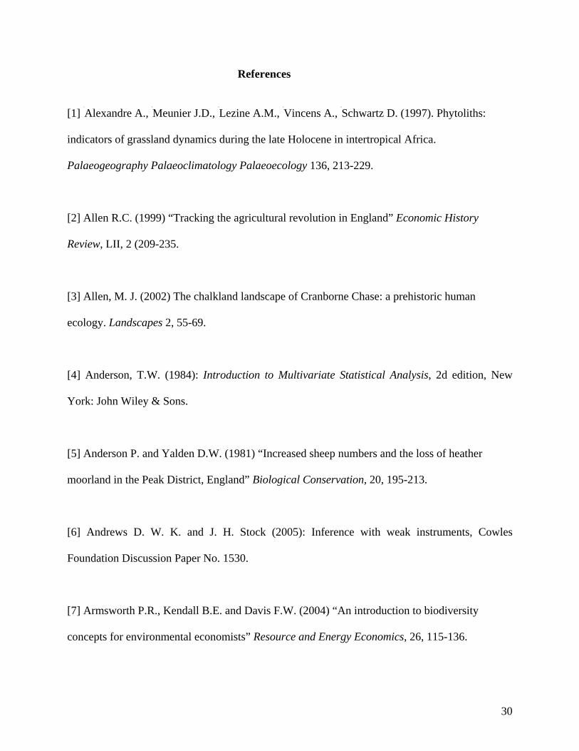
References
[1]
1H
Alexandre A., 2H
Meunier J.D., 3H
Lezine A.M., 4H
Vincens A., 5H
Schwartz D. (1997). Phytoliths:
indicators of grassland dynamics during the late Holocene in intertropical Africa.
Palaeogeography Palaeoclimatology Palaeoecology 136, 213-229.
[2] Allen R.C. (1999) “Tracking the agricultural revolution in England” Economic History
Review, LII, 2 (209-235.
[3] Allen, M. J. (2002) The chalkland landscape of Cranborne Chase: a prehistoric human
ecology. Landscapes 2, 55-69.
[4] Anderson, T.W. (1984): Introduction to Multivariate Statistical Analysis, 2d edition, New
York: John Wiley & Sons.
[5] Anderson P. and Yalden D.W. (1981) “Increased sheep numbers and the loss of heather
moorland in the Peak District, England” Biological Conservation, 20, 195-213.
[6] Andrews D. W. K. and J. H. Stock (2005): Inference with weak instruments, Cowles
Foundation Discussion Paper No. 1530.
[7] Armsworth P.R., Kendall B.E. and Davis F.W. (2004) “An introduction to biodiversity
concepts for environmental economists” Resource and Energy Economics, 26, 115-136.
31
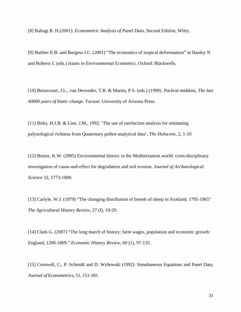
[8] Baltagi B. H.(2001): Econometric Analysis of Panel Data, Second Edition, Wiley.
[9] Barbier E.B. and Burgess J.C. (2001) “The economics of tropical deforestation” in Hanley N
and Roberts C (eds.) Issues in Environmental Economics. Oxford: Blackwells.
[10] Betancourt, J.L., van Devender, T.R. & Martin, P.S. (eds.) (1990). Packrat middens, The last
40000 years of biotic change. Tucson: University of Arizona Press.
[11] Birks, H.J.B. & Line, J.M., 1992. ‘The use of rarefaction analysis for estimating
palynological richness from Quaternary pollen-analytical data’, The Holocene, 2, 1-10.
[12] Butzer, K.W. (2005) Environmental history in the Mediterranean world: cross-disciplinary
investigation of cause-and-effect for degradation and soil erosion. Journal of Archaeological
Science 32, 1773-1800.
[13] Carlyle, W.J. (1979) “The changing distribution of breeds of sheep in Scotland, 1795-1965”
The Agricultural History Review, 27 (I), 19-29.
[14] Clark G. (2007) “The long march of history: farm wages, population and economic growth:
England, 1200-1869.” Economic History Review, 60 (1), 97-135.
[15] Cornwell, C., P. Schmidt and D. Wyhowski (1992): Simultaneous Equations and Panel Data,
Journal of Econometrics, 51, 151-181.
32
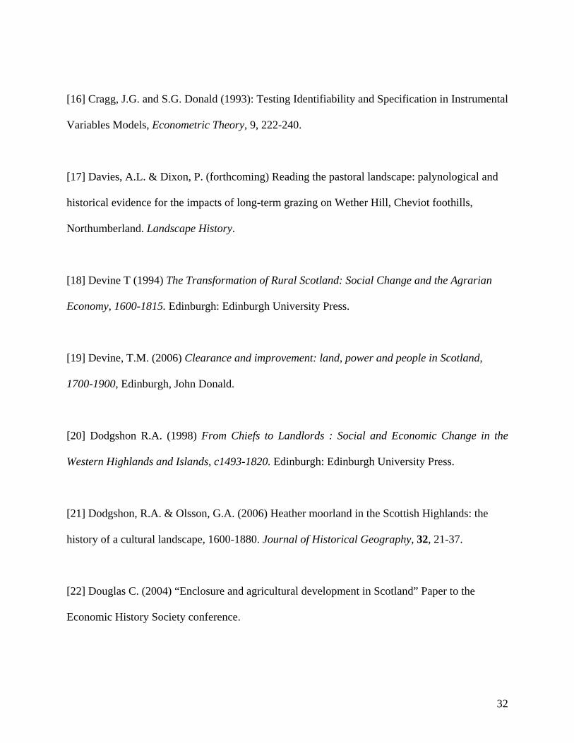
[16] Cragg, J.G. and S.G. Donald (1993): Testing Identifiability and Specification in Instrumental
Variables Models, Econometric Theory, 9, 222-240.
[17] Davies, A.L. & Dixon, P. (forthcoming) Reading the pastoral landscape: palynological and
historical evidence for the impacts of long-term grazing on Wether Hill, Cheviot foothills,
Northumberland. Landscape History.
[18] Devine T (1994) The Transformation of Rural Scotland: Social Change and the Agrarian
Economy, 1600-1815. Edinburgh: Edinburgh University Press.
[19] Devine, T.M. (2006) Clearance and improvement: land, power and people in Scotland,
1700-1900, Edinburgh, John Donald.
[20] Dodgshon R.A. (1998) From Chiefs to Landlords : Social and Economic Change in the
Western Highlands and Islands, c1493-1820. Edinburgh: Edinburgh University Press.
[21] Dodgshon, R.A. & Olsson, G.A. (2006) Heather moorland in the Scottish Highlands: the
history of a cultural landscape, 1600-1880. Journal of Historical Geography, 32, 21-37.
[22] Douglas C. (2004) “Enclosure and agricultural development in Scotland” Paper to the
Economic History Society conference.
33
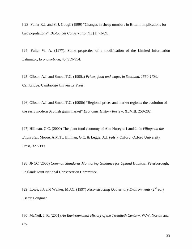
[ 23] Fuller R.J. and S. J. Gough (1999) “Changes in sheep numbers in Britain: implications for
bird populations”. Biological Conservation 91 (1) 73-89.
[24] Fuller W. A. (1977): Some properties of a modification of the Limited Information
Estimator, Econometrica, 45, 939-954.
[25] Gibson A.J. and Smout T.C. (1995a) Prices, food and wages in Scotland, 1550-1780.
Cambridge: Cambridge University Press.
[26] Gibson A.J. and Smout T.C. (1995b) “Regional prices and market regions: the evolution of
the early modern Scottish grain market” Economic History Review, XLVIII, 258-282.
[27] Hillman, G.C. (2000) The plant food economy of Abu Hureyra 1 and 2. In Village on the
Euphrates, Moore, A.M.T., Hillman, G.C. & Legge, A.J. (eds.). Oxford: Oxford University
Press, 327-399.
[28] JNCC (2006) Common Standards Monitoring Guidance for Upland Habitats. Peterborough,
England: Joint National Conservation Committee.
[29] Lowe, J.J. and Walker, M.J.C. (1997) Reconstructing Quaternary Environments (2nd ed.)
Essex: Longman.
[30] McNeil, J. R. (2001) An Environmental History of the Twentieth Century. W.W. Norton and
Co..
34
[31] Midgley, A.C. (2006) The social negotiation of nature conservation policy: conserving
pinewoods in the Scottish Highlands. Biodiversity and Conservation DOI 10.1007/s10531-006-
9133-7.
[32] Moore, P.D. (2005) Palaeoecology - Down to the Woods Yesterday. Nature 433, 588-589.
[33] Orians GH and Soule ME (2001) “Introduction” in Orians and Soule (eds) Conservation
Biology: Priorities for the next decade”: Washington DC: Island Press.
[34] Palmer, S.C.F. (1997). Prediction of the shoot production of heather under grazing in the
uplands of Great Britain. Grass and Forage Science 52, 408-424.
[35] Shapiro, S. S. and M. B. Wilk (1965): An analysis of variance test for normality, Biometrika,
52, 591-641.
[36] Shea, J. (1997): Instrument relevance in multivariate linear models: A simple measure,
Review of Economics and Statistics, 49, 348-352.
[37] Simmons A (1998) Burt’s Letters from the north of Scotland. Edinburgh: Birlinn Press.
[38] Simmons I. (2001) An environmental history of Great Britain from 10,000 years ago to the
present. Edinburgh: Edinburgh University Press.
35
[39] Simpson, I.A., Dugmore, A.J., Thomson, A. & Vesteinsson, O. (2001) Crossing the
thresholds: human ecology and historical patterns of landscape degradation. Catena, 42, 175-192.
[40] Smout, TC (1985) A History of the Scottish People, 1560-1830, London: Fontana.
[41] Smout T.C. (2000) Nature Contested: environmental history in Scotland and Northern
England since 1600. Edinburgh: Edinburgh University Press.
[42] Stevenson, A.C. and Thompson, D.B.A. (1993) Long-term changes in the extent of heather
moorland in upland Britain and Ireland: palaeoecological evidence for the importance of grazing.
The Holocene, 3, 70-76.
[43] Stock, J. H. and M. Yogo (2005): Testing for Weak Instruments in Linear IV Regression,
Ch.5 in J.H. Stock and D.W.K. Andrews (eds), Identification and Inference for Econometric
Models: Essays in Honor of Thomas J. Rothenberg, Cambridge University Press.
[44] Sutherland W. and Hill D. (1995) Managing Habitats for Conservation. Cambridge:
Cambridge University Press.
[45] Thompson D.B.A., MacDonald A.J. and Galbraith C.A. (1995) “Upland heather moorland in
Great Britain: a review of international importance, vegetation change and some objectives for
nature conservation” Biological Conservation, 71, 163-178.
36
[46] Tipping, R. (2000) Palaeoecological approaches to historical problems: a comparison of
sheep-grazing intensities in the Cheviot hills in the medieval and later periods. In Townships to
Farmsteads: Rural Settlement Studies in Scotland, England and Wales (ed. by Atkinson, J.,
Banks, I. & MacGregor, G.). British Archaeological Reports (British Series), 293, 130-143.
[47] Tipping, R. (2004) Palaeoecology and political history; evaluating driving forces in historic
landscape change in southern Scotland. In Society, Landscape and Environment in Upland
Britain, Whyte, I.D. & Winchester, A.J.L. (eds.), pp. 11-20. Society for Landscape Studies
supplementary series 2.
[48] Whyte I (1979) Agriculture and Society in Seventeenth Century Scotland. Edinburgh: John
Donald Publishers Ltd.
[49] Wilson E.O. (1988) Biodiversity. Washington DC: National Academy Press.
[50] Wooldridge J. (2002) Econometric analysis of cross section and panel data” . Cambridge.,
Ma. :MIT Press.
[51] Worster D. (1993) Wealth of Nature: Environmental History and the Ecological
Imagination. Oxford: Oxford University Press.
[52] Worster D. (1988) The Ends of the Earth: perspectives on modern environmental history.
Cambridge: Cambridge University Press.
37
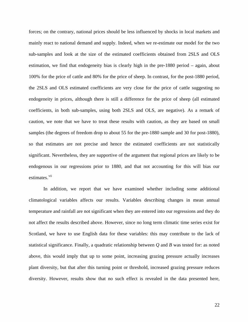
Figure 1. Locations of all sites investigated in project. Breadalbane Estate: (1) Leadour farm & shieling, Loch Tay,
(2) Corries shieling, Glenorchy; Sutherland Estate: (3) Glenleraig farm & shieling, Assynt, (4) Rogart farm & shieling, Sutherland; Buccleuch Estate: (5) Bush of Ewes farm, Ewesdale, (6) Greenshiels shieling/farm, Liddesdale; Grant of Freuchy Estate: (7) Rynuie farm/shieling, Abernethy.
38
-2000
-1900
-1800
-1700
-1600
Sample
age (
calen
dar y
ears
AD)
10
15
20
25
30
35
40
45
Depth
(cm be
low gr
ound
surfa
ce)
20
Alnus g
lutino
sa (a
lder)
20
Betula
(birch
)
20
Pinus s
ylves
tris (S
cots
pine)
20
Myrica
gale
(bog m
yrtle)
20
Callun
a vulg
aris (
heath
er)
20 40 60
Poace
ae (g
rass)
Avena
/Triti
cum gr
oup (
oats/
wheat)
Hordeu
m grou
p (e.g
. barl
ey)
20Cyp
erac
eae (
sedg
es)
Achille
a-typ
e (e.g
. yarr
ow)
Cichori
um in
tybus
-type
(e.g.
dand
elion
)
Plantag
o lan
ceola
ta (rib
wort p
lantai
n)
20
Potenti
lla-ty
pe (e
.g. to
rmen
til)
20
Ranun
culus
acris
-type
(butt
ercu
p)
Silene
vulga
ris-ty
pe (c
ampio
n)
Solida
go vi
rgaure
a-typ
e (e.g
. dais
y)
50 100 150
Charco
al su
m
20 40 60 80 100
Trees
Shrubs
Heaths
Herbs
Zone
GLE2c
GLE2b
GLE2a
GLE1b
GLE1a
Trees & shrubs Heaths & herbs
Analyst: A.L.Davies Figure 2. Selected percentage pollen data for Glenleraig farm, Assynt, c.1600 to present. The clear curve shows a x10 exaggeration for clarity. Horizontal lines (zones) depict periods of vegetation change (e.g. GLE1 farm occupation, GLE2a settlement abandonment for intensive sheep grazing, GLE2b-c less grazing), which are also recorded in the diversity analyses (see Figure 3).
39
0
5
10
15
20
25
30
35
40
160016501700175018001850190019502000
Age (AD)
Estim
ated
pal
ynol
ogic
al ri
chne
ss
Glenleraig farmFarm meanRuigh Dorch shielingShieling mean
Figure 3: Estimated pollen diversity over time for two sites in Assynt, c.1600 to present.
40
Table One – Variables in data base
Variable Name, and Acronym if used in main model
Meaning Main sources Type of data
Dependent Variable: Diversity, Bit estimated species count at site i in year t Pollen analysis Continuous Explanatory Variables: Lagged diversity, Bit-1 Species diversity estimate in previous 20
year period Pollen analysis Continuous
Site management intensity mginten
Intensity of use through year (5=year round; 1= abandoned)
Estate records Categorical
Size change, sizechange
Property amalgamation or split Estate records Count of occurrences per 20 yr period
Management change, mgtchange
Eg enclosures, draining Estate records Count of occurrences per 20 year period
Animal issues 1, andisease
Disease Estate records Yes/no in 20 year period
Animal issues 2, annewbreed
New breeds introduced Estate records Yes/no in 20 year period
Prices Sheep, psheep Regional market price Estate records; Royal
Highland Agricultural Society,
In £/240
Cattle, pcattle Regional market price Estate records; Royal Highland Agricultural Society
In £/240
Environmental Temperature Mean monthly English data Degrees C Rainfall total annual English data Mm Extreme weather events, extrweather
Storms, floods unusual enough to be recorded.
Estate records Count during 20 year period
Other Extreme civil events, extrcivil
War, disease, famine etc Estate records Count during 20 year period
Demand Drivers for use as instruments
Bere (barley) price, pbere
Regional market price Fiars data, estate records In £/240
garrison Whether a military garrison was stationed in the area
Historical Fact Yes/No

41
union Act of Union between Scotland and England enacted
Historical Fact Yes/No
refrigeration Introduction of refrigerated transport. Historical Fact Yes/No popenglish Population of England Pre 1800: expert opinion
Post 1800: Census Count
42
TABLE 2: The effect of economic activity on biodiversity (livestock prices)
Dep. variable:
Biodiversity index (Bt)
(1) 2SLS
(2) Fuller-LIML
(3) 2SLS
(4) Fuller-LIML
(5) Fuller- LIML
(6) Fuller- LIML
Bt-1 0.571** (3.93)
0.571** (3.88)
0.576** (3.93)
0.576** (3.86)
0.580** (3.92)
0.586** (3.91)
pcattle -0.006** (-2.16)
-0.006** (-2.16)
- - -0.006** (-2.06)
-
psheep - - -0.078** (-2.07)
-0.078** (-2.06)
- -0.074** (-1.97)
sizechange 0.599 (0.53)
0.599 (0.53)
0.581 (0.51)
0.581 (0.51)
- -
mgtchange -0.090 (-0.40)
-0.091 (-0.40)
-0.075 (-0.33)
-0.076 (-0.34)
- -
andisease -0.615 (-0.56)
-0.619 (-0.56)
-0.581 (-0.53)
-0.583 (-0.53)
- -
annewbread 1.628 (1.15)
1.626 (1.15)
1.638 (1.15)
1.637 (1.15)
1.343 (1.09)
1.374 (1.11)
mgtinten 0.517** (2.32)
0.516** (2.31)
0.506** (2.25)
0.505** (2.24)
0.505** (2.34)
0.494** (2.26)
extrweather -0.228 (-0.62)
-0.228 (-0.62)
-0.218 (-0.60)
-0.219 (-0.60)
- -
extrcivil -0.093 (-0.13)
-0.093 (-0.13)
-0.109 (-0.15)
-0.109 (-0.17)
- -
constant 7.784** (2.49)
7.784** (2.46)
7.738** (2.43)
7.741** (2.39)
7.557** (2.37)
7.502** (2.30)
43
Sargan over-identification test
2)4(χ = 2.509
(0.643)
2)4(χ = 2.509
(0.643)
2)4(χ = 2.845
(0.584)
2)4(χ = 2.840
(0.584)
2)4(χ = 1.418
(0.841)
2)4(χ = 1.731
(0.785) Anderson canonical
correlations 2
)5(χ = 38.52 (0.000)
2)5(χ = 38.07
(0.000)
2)5(χ = 37.20
(0.000)
2)5(χ = 36.88
(0.000) Cragg-Donald
under-identification 2
)5(χ = 45.48 (0.000)
2)5(χ = 44.87
(0.000)
2)5(χ = 43.67
(0.000)
2)5(χ = 43.23
(0.000) Stock-Yogo weak
identification 6.05
(9.48) 6.05
(5.34) 5.97
(9.48) 5.97
(5.34) 6.12
(5.34) 6.05
(5.34) First-stage
F (Bt-1) )95,6(F = 8.99
(0.000) )95,6(F = 8.99
(0.000) )100,6(F = 9.37
(0.000) )100,6(F = 9.37
(0.000) First-stage F (prices)
)95,6(F =115.45 (0.000)
)95,6(F = 114.07 (0.000)
)100,6(F =117.3 (0.000)
)100,6(F = 116.17 (0.000)
Shea partial 2R (Bt-1) 0.277 0.274 0.269 0.267
Shea partial 2R (prices)
0.672 0.665 0.654 0.648
SW normality test 0.992 (0.751)
0.992 (0.753)
0.992 (0.737)
0.992 (0.740)
0.993 (0.846)
0.993 (0.823)
Notes:1. There are 119 observations. All regressions include dummies for each site. 2. The instruments used are Bt-2, popenglish, garrison, union, refrigeration, pbere. 3. t-ratios are shown in parentheses below the estimated coefficients. An asterisk denotes significance at the 10% level and two asterisks at the 5% level. 2. LIML is Fuller’s (1977) modified LIML with a=1. 5. The Sargan test is a test of overidentifying restrictions. Under the null, the test statistic is distributed as chi-squared in the number of overidentifying restrictions (the p-value is reported in parenthesis). 6. The Anderson (1984) canonical correlations is a likelihood-ratio test of whether the equation is identified. The Cragg and Donald (1993) test statistic is also a chi-squared test of whether the equation is identified. Under the null of underidentification, the statistics are distributed as chi-squared with degrees of freedom=(L-K+1) where L=number of instruments (included + excluded) and K is the number of regressors (the p-values are reported in parentheses). 7. The Stock and Yogo statistic is used to test for the presence of weak instruments (i.e., that the equation is only weakly identified). The critical value for a 10% bias in 2SLS is reported in parentheses (see Stock and Yogo (2005) for a tabulation of critical values). 8. The 1st stage F-statistic tests the hypothesis that the coefficients on all the excluded instruments are zero in the 1st stage regression of the endogenous regressor on all instruments (the p-value is reported in parenthesis). 9. Shea's (1997) "partial R-squared" is a measure of instrument relevance that takes into account intercorrelations among instruments. 10. The SW is the Shapiro and Wilk (1965) test for normality, for the residuals of the structural equation. The p-value of the test is reported in parentheses.
44
TABLE 3: The effect of economic activity on biodiversity (relative prices)
Dep. variable:
Biodiversity index (Bt)
(1) 2SLS
(2) Fuller-LIML
(3) 2SLS
(4) Fuller-LIML
(5) Fuller- LIML
(6) Fuller- LIML
Bt-1 0.592** (3.96)
0.592** (3.95)
0.601** (3.95)
0.601** (3.93)
0.607** (4.08)
0.614** (4.05)
pcattle/pbere -0.002* (-1.84)
-0.002* (-1.84)
- - -0.002* (-1.66)
-
psheep/pbere - - -0.030* (-1.70)
-0.031* (-1.70)
- -0.027 (-1.55)
sizechange 0.629 (0.56)
0.629 (0.56)
0.571 (0.50)
0.572 (0.50)
- -
mgtchange -0.100 (-0.45)
-0.100 (-0.45)
-0.065 (-0.33)
-0.065 (-0.29)
- -
andisease -0.655 (-0.59)
-0.655 (-0.59)
-0.571 (-0.51)
-0.572 (-0.51)
- -
annewbread 1.601 (1.14)
1.601 (1.14)
1.602 (1.12)
1.602 (1.12)
1.03 (0.97)
1.305 (1.04)
mgtinten 0.442* (1.90)
0.442* (1.90)
0.421* (1.74)
0.420* (1.73)
0.447** (1.98)
0.424* (1.79)
extrweather -0.261 (-0.72)
-0.261 (-0.72)
-0.249 (-0.68)
-0.249 (-0.68)
- -
extrcivil -0.117 (-0.17
-0.117 (-0.17
-0.157 (-0.22)
-0.157 (-0.22)
- -
constant 7.771** (2.27)
7.764** (2.26)
7.727** (2.16)
7.723** (2.14)
7.778** (2.14)
7.729** (2.04)
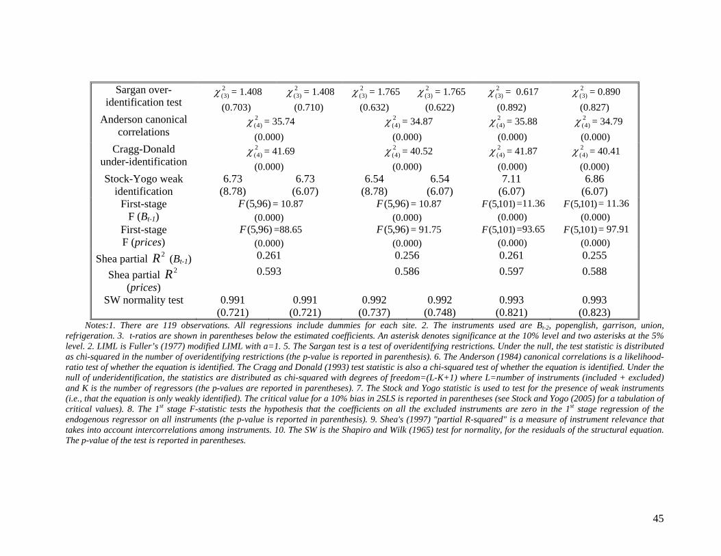
45
Sargan over-identification test
2)3(χ = 1.408
(0.703)
2)3(χ = 1.408
(0.710)
2)3(χ = 1.765
(0.632)
2)3(χ = 1.765
(0.622)
2)3(χ = 0.617
(0.892)
2)3(χ = 0.890
(0.827) Anderson canonical
correlations 2
)4(χ = 35.74 (0.000)
2)4(χ = 34.87
(0.000)
2)4(χ = 35.88
(0.000)
2)4(χ = 34.79
(0.000) Cragg-Donald
under-identification 2
)4(χ = 41.69 (0.000)
2)4(χ = 40.52
(0.000)
2)4(χ = 41.87
(0.000)
2)4(χ = 40.41
(0.000) Stock-Yogo weak
identification 6.73
(8.78) 6.73
(6.07) 6.54
(8.78) 6.54
(6.07) 7.11
(6.07) 6.86
(6.07) First-stage
F (Bt-1) )96,5(F = 10.87
(0.000) )96,5(F = 10.87
(0.000) )101,5(F =11.36
(0.000) )101,5(F = 11.36
(0.000) First-stage F (prices)
)96,5(F =88.65 (0.000)
)96,5(F = 91.75 (0.000)
)101,5(F =93.65 (0.000)
)101,5(F = 97.91 (0.000)
Shea partial 2R (Bt-1) 0.261 0.256 0.261 0.255
Shea partial 2R (prices)
0.593 0.586 0.597 0.588
SW normality test 0.991 (0.721)
0.991 (0.721)
0.992 (0.737)
0.992 (0.748)
0.993 (0.821)
0.993 (0.823)
Notes:1. There are 119 observations. All regressions include dummies for each site. 2. The instruments used are Bt-2, popenglish, garrison, union, refrigeration. 3. t-ratios are shown in parentheses below the estimated coefficients. An asterisk denotes significance at the 10% level and two asterisks at the 5% level. 2. LIML is Fuller’s (1977) modified LIML with a=1. 5. The Sargan test is a test of overidentifying restrictions. Under the null, the test statistic is distributed as chi-squared in the number of overidentifying restrictions (the p-value is reported in parenthesis). 6. The Anderson (1984) canonical correlations is a likelihood-ratio test of whether the equation is identified. The Cragg and Donald (1993) test statistic is also a chi-squared test of whether the equation is identified. Under the null of underidentification, the statistics are distributed as chi-squared with degrees of freedom=(L-K+1) where L=number of instruments (included + excluded) and K is the number of regressors (the p-values are reported in parentheses). 7. The Stock and Yogo statistic is used to test for the presence of weak instruments (i.e., that the equation is only weakly identified). The critical value for a 10% bias in 2SLS is reported in parentheses (see Stock and Yogo (2005) for a tabulation of critical values). 8. The 1st stage F-statistic tests the hypothesis that the coefficients on all the excluded instruments are zero in the 1st stage regression of the endogenous regressor on all instruments (the p-value is reported in parenthesis). 9. Shea's (1997) "partial R-squared" is a measure of instrument relevance that takes into account intercorrelations among instruments. 10. The SW is the Shapiro and Wilk (1965) test for normality, for the residuals of the structural equation. The p-value of the test is reported in parentheses.
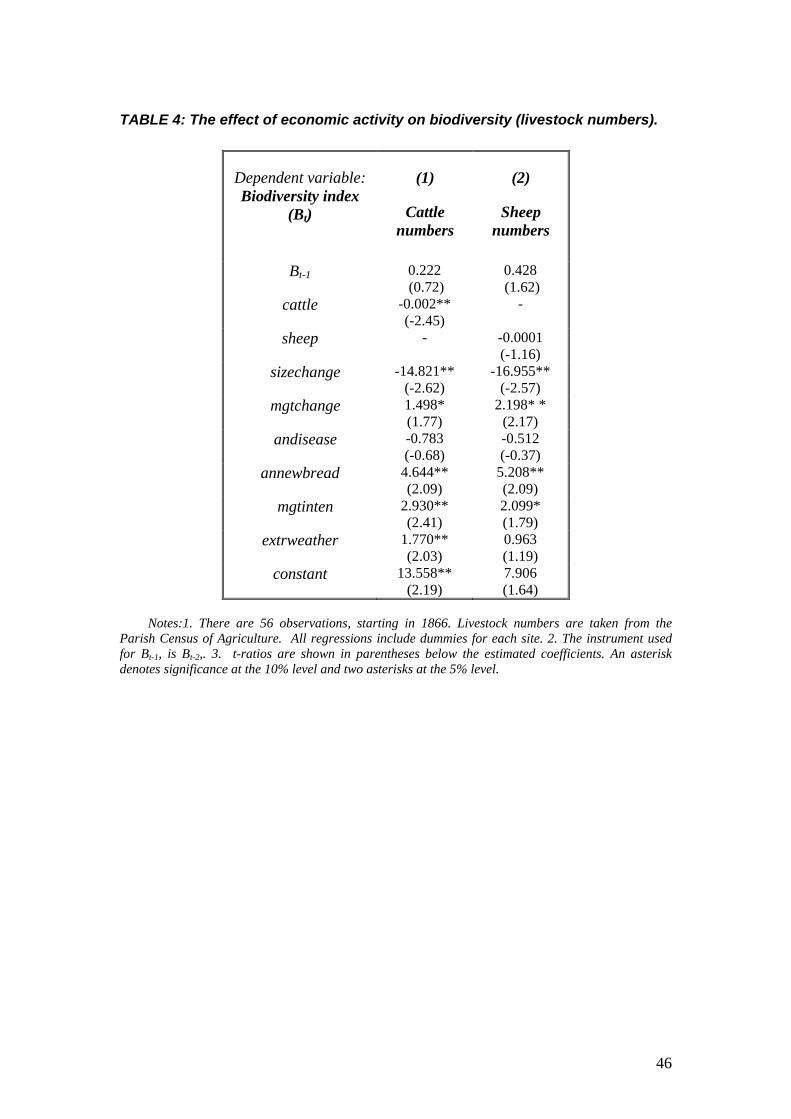
46
TABLE 4: The effect of economic activity on biodiversity (livestock numbers).
Dependent variable: Biodiversity index
(Bt)
(1)
Cattle numbers
(2)
Sheep numbers
Bt-1 0.222 (0.72)
0.428 (1.62)
cattle -0.002** (-2.45)
-
sheep - -0.0001 (-1.16)
sizechange -14.821** (-2.62)
-16.955** (-2.57)
mgtchange 1.498* (1.77)
2.198* * (2.17)
andisease -0.783 (-0.68)
-0.512 (-0.37)
annewbread 4.644** (2.09)
5.208** (2.09)
mgtinten 2.930** (2.41)
2.099* (1.79)
extrweather 1.770** (2.03)
0.963 (1.19)
constant 13.558** (2.19)
7.906 (1.64)
Notes:1. There are 56 observations, starting in 1866. Livestock numbers are taken from the
Parish Census of Agriculture. All regressions include dummies for each site. 2. The instrument used for Bt-1, is Bt-2,. 3. t-ratios are shown in parentheses below the estimated coefficients. An asterisk denotes significance at the 10% level and two asterisks at the 5% level.
47
DATA APPENDIX
Site Data
Site data was gathered for (i) the biodiversity indicator (ii) the variables used in the
“full” model reported in Table 2 of the paper and (iii) variables used as instruments in
the estimation of Table 2. All of these data are shown below as Table A1, and may be
downloaded from:
6Hhttp://www.economics.stir.ac.uk/People/staff/Hanley/hanley.htm.
The dependent variable is Bit, the estimated number of plant species present at site i
in time period t , obtained using palynological analysis of pollen remains in peat
layers dated using a combination of carbon 14 and lead 210 dating. The diversity
estimate was derived by applying rarefaction analysis to each of the pollen sequences
[11]. This differs from ecological measures of biodiversity in that it incorporates a
measure of both plant diversity and vegetation evenness, bearing in mind that not all
pollen types can be identified to species level and that identical diversity values do not
necessarily indicate identical plant assemblages.
“Time period” below refers to a 20 year interval. The independent variables are:
pcattle and psheep, cattle and sheep prices obtained for each region in which sites are
located from entries in estate papers deposited and held in the National Archives of
Scotland. Averages were obtained where multiple entries existed for a given site in a
given time period. Detailed source files for these data, with GD Numbers, are
available from the authors on request.
48
Sizechange is a count variable on the number of recorded instances when the area of
the farm changed, either due to amalgamation with a nearby farm or due to the
breaking up of estates. Information was again obtained from estate papers held largely
in the National Archives.
Mgtchange is a count variable which represents changes such as enclosure and large-
scale draining, again associated with the multiple major changes that formed part of
the Improvement period, but also allowing us to trace the potential effects of small-
scale change in other periods. Information was again obtained from estate papers held
largely in the National Archives.
annewbreed is a dummy variable measuring the introduction, if any, at a given site of
a new breed of sheep or cattle. Information was again obtained from estate papers
held largely in the National Archives.
andisease is a dummy variable measuring whether a serious disease outbreak was
recorded at the site in a given time period. Information was again obtained from estate
papers held largely in the National Archives.
Mginten is a categorical variable which records the extent to which the site was used
year-round for agriculture by the tenant farmer. A value of 5 means the site was used
year-round (eg the grazing paddocks or “in bye” land closest to the farm steading), a
value of 4 that the site was a summer shieling, 3 that the site was abandoned by the
tenant but still occasionally cropped (a very infrequent event in the data), 2 that the
site was abandoned but still occasionally grazed, and 1 that the site was completely
abandoned from agricultural use.
Extrweather is a count variable which records how often the site documents discuss
an “extreme weather event”, such as a flood, drought or heavy snowfall, during the
time period.
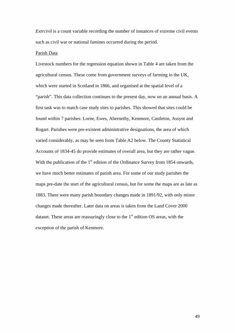
49
Extrcivil is a count variable recording the number of instances of extreme civil events
such as civil war or national famines occurred during the period.
Parish Data
Livestock numbers for the regression equation shown in Table 4 are taken from the
agricultural census. These come from government surveys of farming in the UK,
which were started in Scotland in 1866, and organised at the spatial level of a
“parish”. This data collection continues to the present day, now on an annual basis. A
first task was to match case study sites to parishes. This showed that sites could be
found within 7 parishes: Lorne, Ewes, Abernethy, Kenmore, Castleton, Assynt and
Rogart. Parishes were pre-existent administrative designations, the area of which
varied considerably, as may be seen from Table A2 below. The County Statistical
Accounts of 1834-45 do provide estimates of overall area, but they are rather vague.
With the publication of the 1st edition of the Ordinance Survey from 1854 onwards,
we have much better estimates of parish area. For some of our study parishes the
maps pre-date the start of the agricultural census, but for some the maps are as late as
1883. There were many parish boundary changes made in 1891/92, with only minor
changes made thereafter. Later data on areas is taken from the Land Cover 2000
dataset. These areas are reassuringly close to the 1st edition OS areas, with the
exception of the parish of Kenmore.
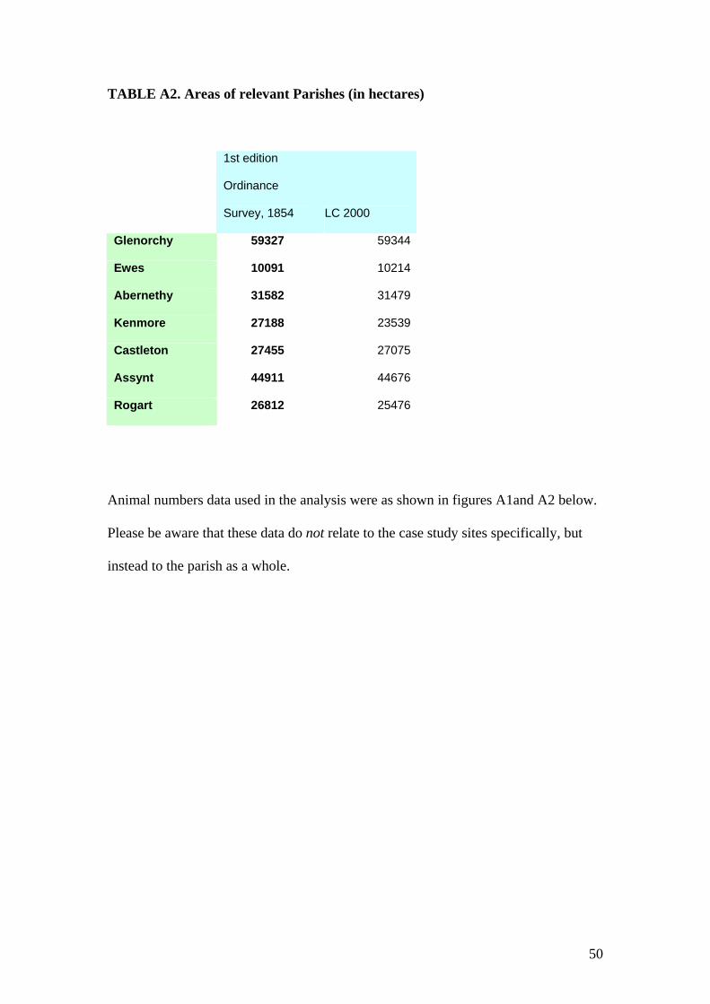
50
TABLE A2. Areas of relevant Parishes (in hectares)
1st edition
Ordinance
Survey, 1854 LC 2000
Glenorchy 59327 59344
Ewes 10091 10214
Abernethy 31582 31479
Kenmore 27188 23539
Castleton 27455 27075
Assynt 44911 44676
Rogart 26812 25476
Animal numbers data used in the analysis were as shown in figures A1and A2 below.
Please be aware that these data do not relate to the case study sites specifically, but
instead to the parish as a whole.
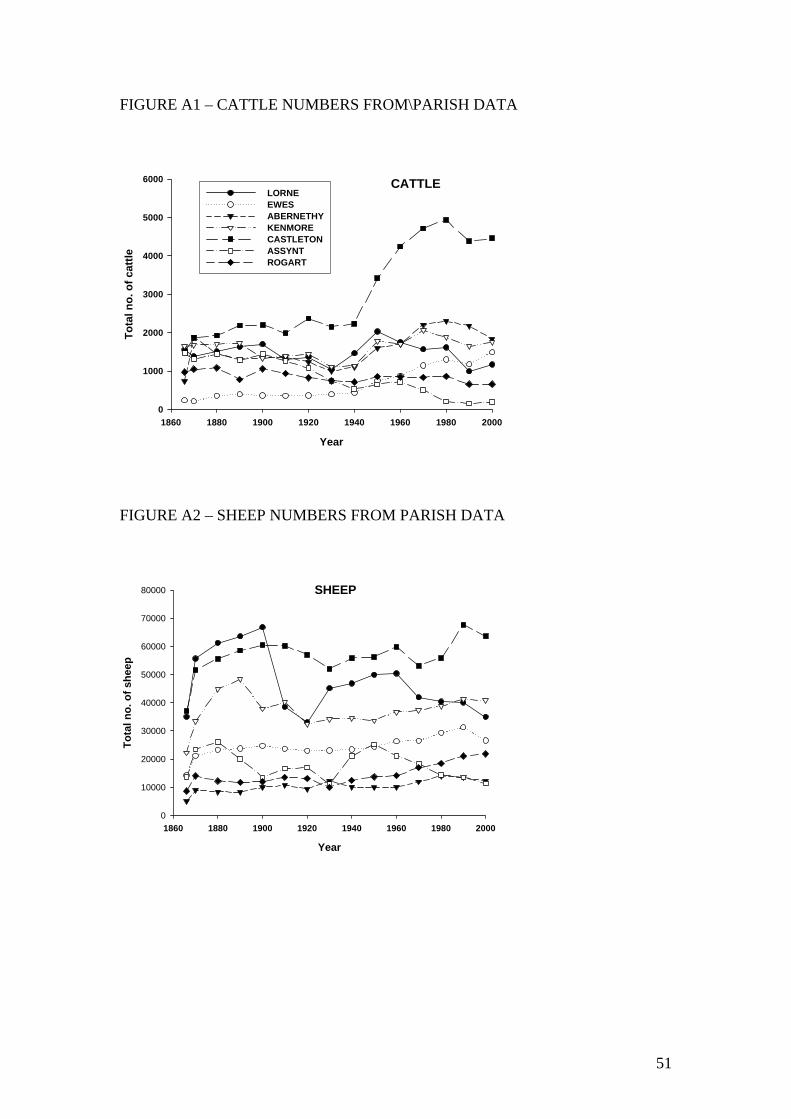
51
FIGURE A1 – CATTLE NUMBERS FROM\PARISH DATA
CATTLE
Year
1860 1880 1900 1920 1940 1960 1980 2000
Tota
l no.
of c
attle
0
1000
2000
3000
4000
5000
6000LORNEEWESABERNETHYKENMORECASTLETONASSYNTROGART
FIGURE A2 – SHEEP NUMBERS FROM PARISH DATA
SHEEP
Year
1860 1880 1900 1920 1940 1960 1980 2000
Tota
l no.
of s
heep
0
10000
20000
30000
40000
50000
60000
70000
80000
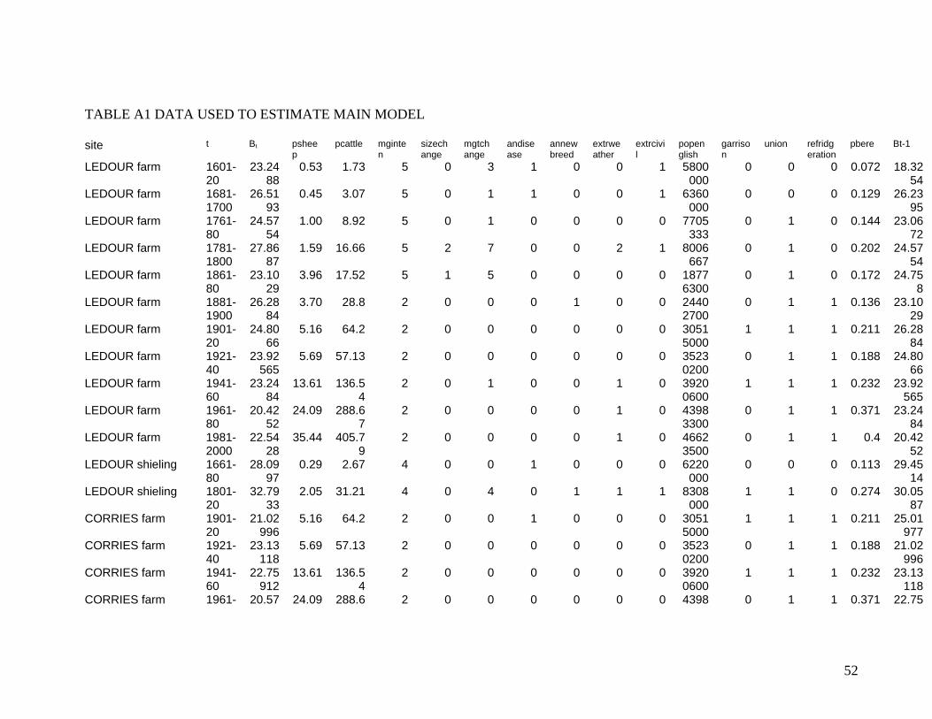
52
TABLE A1 DATA USED TO ESTIMATE MAIN MODEL site t Bt pshee
p pcattle mginte
n sizechange
mgtchange
andisease
annewbreed
extrweather
extrcivil
popenglish
garrison
union refridgeration
pbere Bt-1
LEDOUR farm 1601-20
23.2488
0.53 1.73 5 0 3 1 0 0 1 5800000
0 0 0 0.072 18.3254
LEDOUR farm 1681-1700
26.5193
0.45 3.07 5 0 1 1 0 0 1 6360000
0 0 0 0.129 26.2395
LEDOUR farm 1761-80
24.5754
1.00 8.92 5 0 1 0 0 0 0 7705333
0 1 0 0.144 23.0672
LEDOUR farm 1781-1800
27.8687
1.59 16.66 5 2 7 0 0 2 1 8006667
0 1 0 0.202 24.5754
LEDOUR farm 1861-80
23.1029
3.96 17.52 5 1 5 0 0 0 0 18776300
0 1 0 0.172 24.758
LEDOUR farm 1881-1900
26.2884
3.70 28.8 2 0 0 0 1 0 0 24402700
0 1 1 0.136 23.1029
LEDOUR farm 1901-20
24.8066
5.16 64.2 2 0 0 0 0 0 0 30515000
1 1 1 0.211 26.2884
LEDOUR farm 1921-40
23.92565
5.69 57.13 2 0 0 0 0 0 0 35230200
0 1 1 0.188 24.8066
LEDOUR farm 1941-60
23.2484
13.61 136.54
2 0 1 0 0 1 0 39200600
1 1 1 0.232 23.92565
LEDOUR farm 1961-80
20.4252
24.09 288.67
2 0 0 0 0 1 0 43983300
0 1 1 0.371 23.2484
LEDOUR farm 1981-2000
22.5428
35.44 405.79
2 0 0 0 0 1 0 46623500
0 1 1 0.4 20.4252
LEDOUR shieling 1661-80
28.0997
0.29 2.67 4 0 0 1 0 0 0 6220000
0 0 0 0.113 29.4514
LEDOUR shieling 1801-20
32.7933
2.05 31.21 4 0 4 0 1 1 1 8308000
1 1 0 0.274 30.0587
CORRIES farm 1901-20
21.02996
5.16 64.2 2 0 0 1 0 0 0 30515000
1 1 1 0.211 25.01977
CORRIES farm 1921-40
23.13118
5.69 57.13 2 0 0 0 0 0 0 35230200
0 1 1 0.188 21.02996
CORRIES farm 1941-60
22.75912
13.61 136.54
2 0 0 0 0 0 0 39200600
1 1 1 0.232 23.13118
CORRIES farm 1961- 20.57 24.09 288.6 2 0 0 0 0 0 0 4398 0 1 1 0.371 22.75
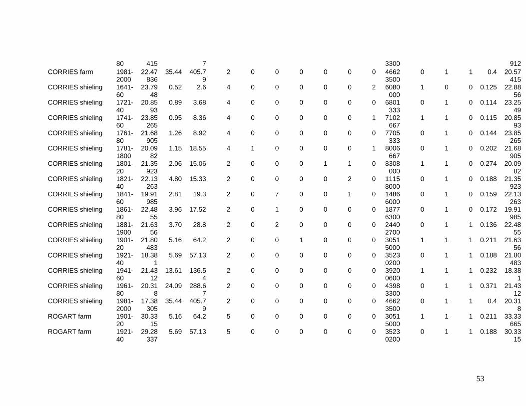
53
80 415 7 3300 912 CORRIES farm 1981-
2000 22.47
836 35.44 405.7
92 0 0 0 0 0 0 4662
35000 1 1 0.4 20.57
415 CORRIES shieling 1641-
60 23.79
48 0.52 2.6 4 0 0 0 0 0 2 6080
0001 0 0 0.125 22.88
56 CORRIES shieling 1721-
40 20.85
93 0.89 3.68 4 0 0 0 0 0 0 6801
3330 1 0 0.114 23.25
49 CORRIES shieling 1741-
60 23.85
265 0.95 8.36 4 0 0 0 0 0 1 7102
6671 1 0 0.115 20.85
93 CORRIES shieling 1761-
80 21.68
905 1.26 8.92 4 0 0 0 0 0 0 7705
3330 1 0 0.144 23.85
265 CORRIES shieling 1781-
1800 20.09
82 1.15 18.55 4 1 0 0 0 0 1 8006
6670 1 0 0.202 21.68
905 CORRIES shieling 1801-
20 21.35
923 2.06 15.06 2 0 0 0 1 1 0 8308
0001 1 0 0.274 20.09
82 CORRIES shieling 1821-
40 22.13
263 4.80 15.33 2 0 0 0 0 2 0 1115
80000 1 0 0.188 21.35
923 CORRIES shieling 1841-
60 19.91
985 2.81 19.3 2 0 7 0 0 1 0 1486
60000 1 0 0.159 22.13
263 CORRIES shieling 1861-
80 22.48
55 3.96 17.52 2 0 1 0 0 0 0 1877
63000 1 0 0.172 19.91
985 CORRIES shieling 1881-
1900 21.63
56 3.70 28.8 2 0 2 0 0 0 0 2440
27000 1 1 0.136 22.48
55 CORRIES shieling 1901-
20 21.80
483 5.16 64.2 2 0 0 1 0 0 0 3051
50001 1 1 0.211 21.63
56 CORRIES shieling 1921-
40 18.38
1 5.69 57.13 2 0 0 0 0 0 0 3523
02000 1 1 0.188 21.80
483 CORRIES shieling 1941-
60 21.43
12 13.61 136.5
42 0 0 0 0 0 0 3920
06001 1 1 0.232 18.38
1 CORRIES shieling 1961-
80 20.31
8 24.09 288.6
72 0 0 0 0 0 0 4398
33000 1 1 0.371 21.43
12 CORRIES shieling 1981-
2000 17.38
305 35.44 405.7
92 0 0 0 0 0 0 4662
35000 1 1 0.4 20.31
8 ROGART farm 1901-
20 30.33
15 5.16 64.2 5 0 0 0 0 0 0 3051
50001 1 1 0.211 33.33
665 ROGART farm 1921-
40 29.28
337 5.69 57.13 5 0 0 0 0 0 0 3523
02000 1 1 0.188 30.33
15
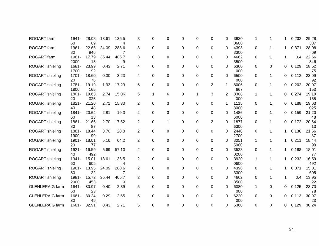
54
ROGART farm 1941-60
28.0869
13.61 136.54
3 0 0 0 0 0 0 39200600
1 1 1 0.232 29.28337
ROGART farm 1961-80
22.66846
24.09 288.67
3 0 0 0 0 0 0 43983300
0 1 1 0.371 28.0869
ROGART farm 1981-2000
17.7918
35.44 405.79
3 0 0 0 0 0 0 46623500
0 1 1 0.4 22.66846
ROGART shieling 1681-1700
23.9992
0.43 2.71 4 0 0 0 0 0 0 6360000
0 0 0 0.129 18.5275
ROGART shieling 1701-20
18.6076
0.30 3.23 4 0 0 0 0 0 0 6500000
0 1 0 0.112 23.9992
ROGART shieling 1781-1800
19.19165
1.93 17.29 5 0 0 0 0 2 1 8006667
0 1 0 0.202 20.97153
ROGART shieling 1801-20
19.63025
2.74 15.06 5 1 6 0 1 3 2 8308000
1 1 0 0.274 19.19165
ROGART shieling 1821-40
21.2048
2.71 15.33 2 0 3 0 0 0 1 11158000
0 1 0 0.188 19.63025
ROGART shieling 1841-60
20.6413
2.81 19.3 2 0 3 0 0 0 0 14866000
0 1 0 0.159 21.2048
ROGART shieling 1861-80
21.6687
2.70 17.52 2 0 1 0 0 2 0 18776300
0 1 0 0.172 20.6413
ROGART shieling 1881-1900
18.4499
3.70 28.8 2 0 0 0 0 0 0 24402700
0 1 1 0.136 21.6687
ROGART shieling 1901-20
18.0177
5.16 64.2 2 0 0 0 0 0 0 30515000
1 1 1 0.211 18.4499
ROGART shieling 1921-40
16.59492
5.69 57.13 2 0 0 0 0 0 0 35230200
0 1 1 0.188 18.0177
ROGART shieling 1941-60
15.01605
13.61 136.54
2 0 0 0 0 0 0 39200600
1 1 1 0.232 16.59492
ROGART shieling 1961-80
13.9522
24.09 288.67
2 0 0 0 0 0 0 43983300
0 1 1 0.371 15.01605
ROGART shieling 1981-2000
15.72453
35.44 405.79
2 0 0 0 0 0 0 46623500
0 1 1 0.4 13.9522
GLENLERAIG farm 1641-60
30.9723
0.40 2.39 5 0 0 0 0 0 0 6080000
1 0 0 0.125 28.7078
GLENLERAIG farm 1661-80
30.2449
0.29 2.65 5 0 0 0 0 0 0 6220000
0 0 0 0.113 30.9723
GLENLERAIG farm 1681- 32.91 0.43 2.71 5 0 0 0 0 0 0 6360 0 0 0 0.129 30.24
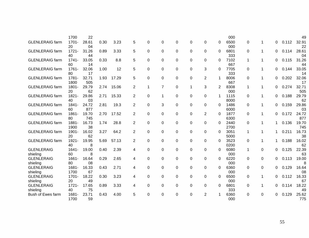
55
1700 22 000 49 GLENLERAIG farm 1701-
20 28.61
04 0.30 3.23 5 0 0 0 0 0 0 6500
0000 1 0 0.112 32.91
22 GLENLERAIG farm 1721-
40 31.26
44 0.89 3.33 5 0 0 0 0 0 0 6801
3330 1 0 0.114 28.61
04 GLENLERAIG farm 1741-
60 33.05
14 0.33 8.8 5 0 0 0 0 0 0 7102
6671 1 0 0.115 31.26
44 GLENLERAIG farm 1761-
80 32.06
17 1.00 12 5 0 0 0 0 3 0 7705
3330 1 0 0.144 33.05
14 GLENLERAIG farm 1781-
1800 32.71
505 1.93 17.29 5 0 0 0 0 2 1 8006
6670 1 0 0.202 32.06
17 GLENLERAIG farm 1801-
20 29.79
62 2.74 15.06 2 1 7 0 1 3 2 8308
0001 1 0 0.274 32.71
505 GLENLERAIG farm 1821-
40 29.86
03 2.71 15.33 2 0 1 0 0 0 1 1115
80000 1 0 0.188 29.79
62 GLENLERAIG farm 1841-
60 24.72
877 2.81 19.3 2 0 3 0 0 0 0 1486
60000 1 0 0.159 29.86
03 GLENLERAIG farm 1861-
80 19.70
745 2.70 17.52 2 0 0 0 0 2 0 1877
63000 1 0 0.172 24.72
877 GLENLERAIG farm 1881-
1900 16.73
38 1.74 28.8 2 0 0 0 0 0 0 2440
27000 1 1 0.136 19.70
745 GLENLERAIG farm 1901-
20 16.02
62 3.27 64.2 2 0 0 0 0 0 0 3051
50001 1 1 0.211 16.73
38 GLENLERAIG farm 1921-
40 19.95
8 5.69 57.13 2 0 0 0 0 0 0 3523
02000 1 1 0.188 16.02
62 GLENLERAIG shieling
1641-60
19.008
0.40 2.39 4 0 0 0 0 0 0 6080000
1 0 0 0.125 22.3963
GLENLERAIG shieling
1661-80
16.6408
0.29 2.65 4 0 0 0 0 0 0 6220000
0 0 0 0.113 19.008
GLENLERAIG shieling
1681-1700
16.3367
0.43 2.71 4 0 0 0 0 0 0 6360000
0 0 0 0.129 16.6408
GLENLERAIG shieling
1701-20
18.2249
0.30 3.23 4 0 0 0 0 0 0 6500000
0 1 0 0.112 16.3367
GLENLERAIG shieling
1721-40
17.6575
0.89 3.33 4 0 0 0 0 0 0 6801333
0 1 0 0.114 18.2249
Bush of Ewes farm 1681-1700
23.7159
0.43 4.00 5 0 0 0 0 2 1 6360000
0 0 0 0.129 25.62775
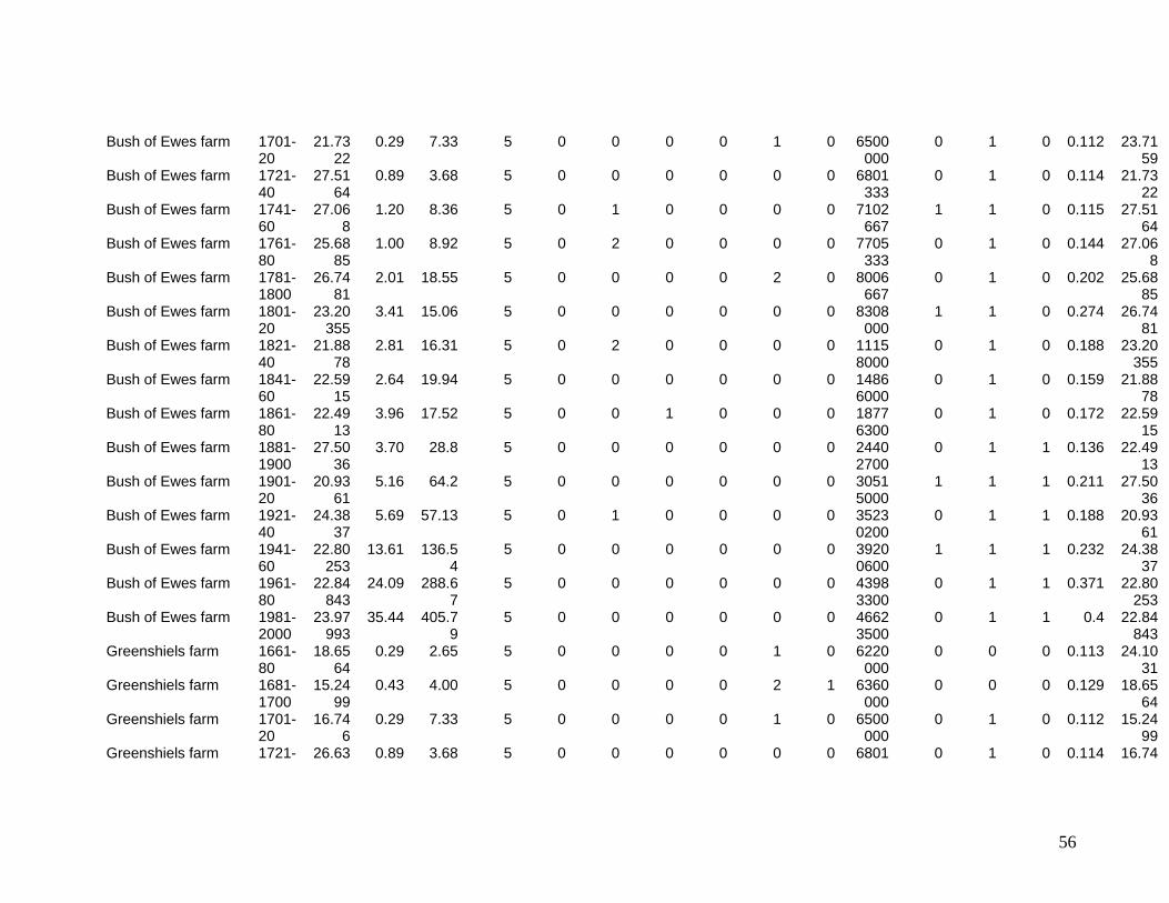
56
Bush of Ewes farm 1701-20
21.7322
0.29 7.33 5 0 0 0 0 1 0 6500000
0 1 0 0.112 23.7159
Bush of Ewes farm 1721-40
27.5164
0.89 3.68 5 0 0 0 0 0 0 6801333
0 1 0 0.114 21.7322
Bush of Ewes farm 1741-60
27.068
1.20 8.36 5 0 1 0 0 0 0 7102667
1 1 0 0.115 27.5164
Bush of Ewes farm 1761-80
25.6885
1.00 8.92 5 0 2 0 0 0 0 7705333
0 1 0 0.144 27.068
Bush of Ewes farm 1781-1800
26.7481
2.01 18.55 5 0 0 0 0 2 0 8006667
0 1 0 0.202 25.6885
Bush of Ewes farm 1801-20
23.20355
3.41 15.06 5 0 0 0 0 0 0 8308000
1 1 0 0.274 26.7481
Bush of Ewes farm 1821-40
21.8878
2.81 16.31 5 0 2 0 0 0 0 11158000
0 1 0 0.188 23.20355
Bush of Ewes farm 1841-60
22.5915
2.64 19.94 5 0 0 0 0 0 0 14866000
0 1 0 0.159 21.8878
Bush of Ewes farm 1861-80
22.4913
3.96 17.52 5 0 0 1 0 0 0 18776300
0 1 0 0.172 22.5915
Bush of Ewes farm 1881-1900
27.5036
3.70 28.8 5 0 0 0 0 0 0 24402700
0 1 1 0.136 22.4913
Bush of Ewes farm 1901-20
20.9361
5.16 64.2 5 0 0 0 0 0 0 30515000
1 1 1 0.211 27.5036
Bush of Ewes farm 1921-40
24.3837
5.69 57.13 5 0 1 0 0 0 0 35230200
0 1 1 0.188 20.9361
Bush of Ewes farm 1941-60
22.80253
13.61 136.54
5 0 0 0 0 0 0 39200600
1 1 1 0.232 24.3837
Bush of Ewes farm 1961-80
22.84843
24.09 288.67
5 0 0 0 0 0 0 43983300
0 1 1 0.371 22.80253
Bush of Ewes farm 1981-2000
23.97993
35.44 405.79
5 0 0 0 0 0 0 46623500
0 1 1 0.4 22.84843
Greenshiels farm 1661-80
18.6564
0.29 2.65 5 0 0 0 0 1 0 6220000
0 0 0 0.113 24.1031
Greenshiels farm 1681-1700
15.2499
0.43 4.00 5 0 0 0 0 2 1 6360000
0 0 0 0.129 18.6564
Greenshiels farm 1701-20
16.746
0.29 7.33 5 0 0 0 0 1 0 6500000
0 1 0 0.112 15.2499
Greenshiels farm 1721- 26.63 0.89 3.68 5 0 0 0 0 0 0 6801 0 1 0 0.114 16.74
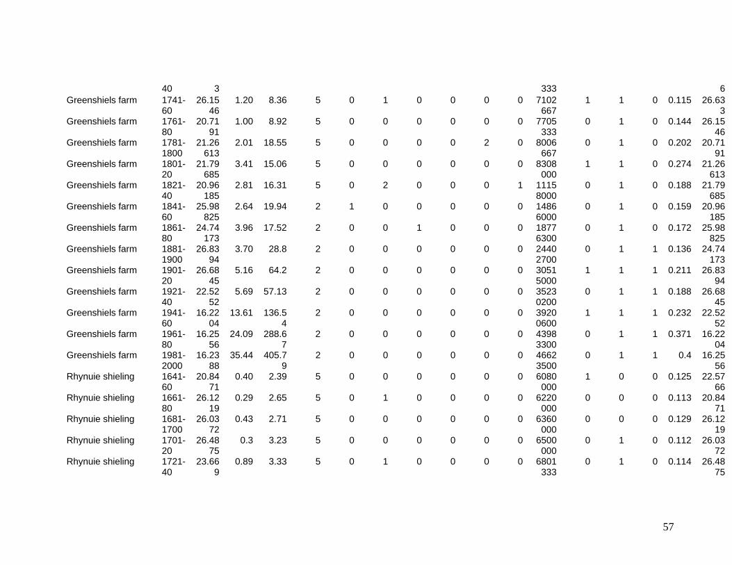
57
40 3 333 6 Greenshiels farm 1741-
60 26.15
46 1.20 8.36 5 0 1 0 0 0 0 7102
6671 1 0 0.115 26.63
3 Greenshiels farm 1761-
80 20.71
91 1.00 8.92 5 0 0 0 0 0 0 7705
3330 1 0 0.144 26.15
46 Greenshiels farm 1781-
1800 21.26
613 2.01 18.55 5 0 0 0 0 2 0 8006
6670 1 0 0.202 20.71
91 Greenshiels farm 1801-
20 21.79
685 3.41 15.06 5 0 0 0 0 0 0 8308
0001 1 0 0.274 21.26
613 Greenshiels farm 1821-
40 20.96
185 2.81 16.31 5 0 2 0 0 0 1 1115
80000 1 0 0.188 21.79
685 Greenshiels farm 1841-
60 25.98
825 2.64 19.94 2 1 0 0 0 0 0 1486
60000 1 0 0.159 20.96
185 Greenshiels farm 1861-
80 24.74
173 3.96 17.52 2 0 0 1 0 0 0 1877
63000 1 0 0.172 25.98
825 Greenshiels farm 1881-
1900 26.83
94 3.70 28.8 2 0 0 0 0 0 0 2440
27000 1 1 0.136 24.74
173 Greenshiels farm 1901-
20 26.68
45 5.16 64.2 2 0 0 0 0 0 0 3051
50001 1 1 0.211 26.83
94 Greenshiels farm 1921-
40 22.52
52 5.69 57.13 2 0 0 0 0 0 0 3523
02000 1 1 0.188 26.68
45 Greenshiels farm 1941-
60 16.22
04 13.61 136.5
42 0 0 0 0 0 0 3920
06001 1 1 0.232 22.52
52 Greenshiels farm 1961-
80 16.25
56 24.09 288.6
72 0 0 0 0 0 0 4398
33000 1 1 0.371 16.22
04 Greenshiels farm 1981-
2000 16.23
88 35.44 405.7
92 0 0 0 0 0 0 4662
35000 1 1 0.4 16.25
56 Rhynuie shieling 1641-
60 20.84
71 0.40 2.39 5 0 0 0 0 0 0 6080
0001 0 0 0.125 22.57
66 Rhynuie shieling 1661-
80 26.12
19 0.29 2.65 5 0 1 0 0 0 0 6220
0000 0 0 0.113 20.84
71 Rhynuie shieling 1681-
1700 26.03
72 0.43 2.71 5 0 0 0 0 0 0 6360
0000 0 0 0.129 26.12
19 Rhynuie shieling 1701-
20 26.48
75 0.3 3.23 5 0 0 0 0 0 0 6500
0000 1 0 0.112 26.03
72 Rhynuie shieling 1721-
40 23.66
9 0.89 3.33 5 0 1 0 0 0 0 6801
3330 1 0 0.114 26.48
75
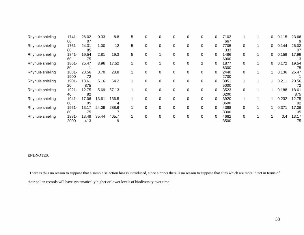
58
Rhynuie shieling 1741-60
26.0207
0.33 8.8 5 0 0 0 0 0 0 7102667
1 1 0 0.115 23.669
Rhynuie shieling 1761-80
24.3185
1.00 12 5 0 0 0 0 0 0 7705333
0 1 0 0.144 26.0207
Rhynuie shieling 1841-60
19.5475
2.81 19.3 5 0 1 0 0 0 0 14866000
0 1 0 0.159 17.9913
Rhynuie shieling 1861-80
25.471
3.96 17.52 1 0 1 0 0 2 0 18776300
0 1 0 0.172 19.5475
Rhynuie shieling 1881-1900
20.5672
3.70 28.8 1 0 0 0 0 0 0 24402700
0 1 1 0.136 25.471
Rhynuie shieling 1901-20
18.61875
5.16 64.2 1 0 0 0 0 0 0 30515000
1 1 1 0.211 20.5672
Rhynuie shieling 1921-40
12.7582
5.69 57.13 1 0 0 0 0 0 0 35230200
0 1 1 0.188 18.61875
Rhynuie shieling 1941-60
17.0605
13.61 136.54
1 0 0 0 0 0 0 39200600
1 1 1 0.232 12.7582
Rhynuie shieling 1961-80
13.1775
24.09 288.67
1 0 0 0 0 0 0 43983300
0 1 1 0.371 17.0605
Rhynuie shieling 1981-2000
13.49413
35.44 405.79
1 0 0 0 0 0 0 46623500
0 1 1 0.4 13.1775
ENDNOTES.
i There is thus no reason to suppose that a sample selection bias is introduced, since a priori there is no reason to suppose that sites which are more intact in terms of
their pollen records will have systematically higher or lower levels of biodiversity over time.
59
ii Samples were taken from small flushes and mires, rather than large blanket peat or raised mire sites in order to provide records which are sensitive to ecological
change on the scale of farm fields.
iii Although we only run the model from 1600 to 2000 due to the lack of historical sources prior to 1600, the pollen data is in fact available back as far as 5500 years
ago for one of our sites. .
iv The 18th century saw the gradual replacement of native sheep breeds in Scotland with two new “imports”: the Cheviot and Blackface sheep. These rapidly spread
through Scotland during the 18th and 19th centuries [13]. Cheviots were favoured for the higher price their wool could command, whilst blackfaced sheep were
hardier than native breeds and could be over-wintered on the hill. Both new breeds also had bigger carcase weights than native breeds. Due to differences in their
grazing behaviour, dry matter intake and length of time on the hill, the introduction of both breeds could be expected to have an effect on plant cover. Cheviots
reached their peak in terms of geographic coverage of Scotland in the 1860s – 1870s, from when they were gradually replaced by blackfaced sheep and cross-
breeds. Their decline is attributed to an over-extension of geographic range, falling wool prices due to imports from Australia and New Zealand, and changing
preferences for sheepmeat. Note that we were unable to model the effects of wool prices due to a lack of data.
v We note that although itB is estimated with 95% confidence intervals, there is no good reason to assume that this measurement error in the dependent variable of
our model is correlated with the independent variables. Hence, there should be no bias in our estimates resulting from this error (see e.g. [50], p.71-72).
vi Our 2SLS estimator here is essentially the fixed effects 2SLS estimator whose properties are discussed in e.g. [15] and [8]).
vii In addition, important biases are introduced in the estimates for the coefficients of prices if we append the site dummies in the error term. Estimating the model
by error-component 2SLS (see [8]), instead of fixed effects 2SLS, results in estimated coefficients for prices of about half the size of those reported in Table 2 –
implying that a random effects panel would also lead to bias.

60