What Education Production Functions Really Show:A Positive Theory of Education Expenditures

Lant Pritchett

Deon Filmer

August 20, 1997

Abstract: The existing empirical work on educational production functions provides powerfulinsights into a positive theory of the allocation of educational expenditures. An optimizingmodel of expenditure allocations predicts that input use should be chosen so that the marginalproduct per dollar of each input is equalized. In decided contrast, the existing literature showsthat the marginal product per dollar of inputs not directly valued by teachers are 10 to 100 timeshigher than that of inputs valued by teachers. This implies that inputs which provide direct benefits to educators (like teacher wages) are vastly over-used relative to inputs that contributedirectly (but only) to educational output (like books or instructional materials). One class ofpositive models of expenditures consistent with this empirical finding invoke a very high ratio ofteacher to parental (or student) influence in the determination of expenditures. This implies thatin some circumstances educational reforms that shift the relative strengths of parents versusteachers in the allocation of expenditures can lead to enormous gains in the cost effectiveness ofschools.

The findings, interpretations, and conclusions expressed in this paper are entirely those of theauthors. They do not necessarily represent the views of the World Bank, its Executive Directors,or the countries they represent. Preliminary draft for comments only, please do not cite withoutpermission of the authors.

We would like to thank Marlaine Lockheed, Emmanuel Jimenez, Elizabeth King, Harold1

Alderman, Michael Kremer, and Jonah Gelbach for helpful comments and discussion.

On the comparison of reading performance of 10 years olds, Venezuela and Indonesia were2

an amazing 6.5 standard deviations below the average of the developed countries. On a similarassessment of science performance of 10 year olds, students from Nigeria and the Philippineswere 2.6 and 3.7 standard deviations below the developed country mean.

August 20, 1997

What Education Production Functions Really Show:Towards a Positive Theory of Education Expenditures1

Introduction

There is broad consensus that expansion in the skills, knowledge, and capacities of

individuals --increasing human capital-- is a key element in economic progress and raising living

standards. Schooling within formal education systems plays an important role in the expansion

of human capital and governments and international fora have often made explicit targets for the

expansion of schooling in enrollment or targets for expenditures. However, there is a big

difference between children sitting in a classroom and an increase in human capital. The quality

of education is a deep concern in many developing countries. On internationally comparable

tests some developing countries, such as Korea and China, do quite well, but others do

abysmally . In some countries students’ achievement test scores after years of instruction are2

little better than random guessing. If these quality deficiencies were due merely to the lack of

inputs the policy prescription would be obvious: increase resources. However, a cumulation of

empirical literature using comparisons of student performance across countries, across regions

within countries, and across schools within regions consistently produces the puzzling and

worrisome finding that resources are only tenuously related to measured achievement.

2

In this paper we build on Hanushek’s (1995) argument that since budget differences do

not account for performance, the incentives that determine how well the budget is spent must

play an important role. We argue the evidence is grossly inconsistent with the assumption that

resources are allocated to maximize educational output (however defined). The key indicator of

this misallocation is that the cost effectiveness, or achievement gain per dollar, of teacher related

inputs is orders of magnitude lower than alternative inputs. Relative overspending on inputs that

are of direct concern to teachers is so pervasive that it is consistent only with a model of the

allocation of education spending in which teacher welfare influences spending, over and above

its impact on school quality.

When performance is more a function of incentives than of spending the policy

implications are less obvious. While in some cases merely increasing the budget is the

appropriate educational policy, it is increasingly recognized that in many other situations more

fundamental reforms that enhance the importance of outputs of education in spending decisions

are necessary (Inter-American Development Bank, 1996).

We want to stress that although we argue that the evidence is consistent with enormous

inefficiencies in education spending due to relatively high spending on teacher inputs, this should

not be construed as an attack on teachers, who are the backbone of any educational system. But

“government” actions are neither deus ex machina nor satanas ex machina, but the result of the

interaction of differing interests. Suggesting that educators defend their interests is a

methodological assumption common to all economics, not an ad hominem attack. Just as there

are “market failures” intrinsic to the incentives of decentralized, uncoordinated exchange, there

are “government failures” which are equally inherent in the structure of incentives created by

Although it should be pointed out this trend in considering market and government failures3

is a renewed, not new, interest for economists:

It is not sufficient to contrast the imperfect adjustments of unfettered private enterprisewith the best adjustment economists in their studies can imagine. For, we cannot expectthat any State authority will attain, or will even whole heartedly seek, that ideal. Suchauthorities are liable alike to ignorance, to sectional pressures, and to personal corruptionby private interest (Pigou, 1912).

3

allocation through the political process . The political pressures on the allocation of expenditures3

across functional categories that we explore here for education are almost certainly present in

other sectors: health clinics with personnel but without drugs or needles, or highways without

maintenance are depressingly common.

I) Theories of the allocation of expenditures

This section first explains why a behavioral theory of expenditure allocation is important

for understanding the results of empirical examinations of the determinants of educational

outcomes. One such theory, an output maximizing model is presented along with three variants:

a simple single educational output, a model with uncertainty, and a model that accommodates

multiple educational outputs. We then introduce an alternative model of expenditure allocations

in which both educational outputs and teacher welfare enter directly into the determination of

spending.

A) Why it takes a theory

Production possibilities are determined by an underlying technological process. The

maximum amount of output possible for an amount of inputs given the constraints imposed by

4

the underlying technical process is the “production function.” The relationship between plant

growth and water or sunlight or fertilizer is determined by a biological process, the relationship

between coal burned and heat produced is determined by a physical process. Similarly, applying

the metaphor to education one can talk of the educational “production function” which is

determined by an underlying pedagogical process.

Even though the production function is derived from technical, not behavioral

relationships, one needs a behavioral theory to understand the results of estimating a production

function for two reasons. First, the increment to output from additional inputs is not constant.

The second algebra book per student will likely help less than the first, and the tenth much less

(perhaps even have a negative impact). The contribution to output of an input depends on the

rate of input utilization at which it is assessed. Nearly all education production function studies

are not experiments in which input use is chosen by a researcher, but rather use data drawn from

reality. In reality, the spending on inputs (e.g. teacher wages, class sizes, buildings, textbook

use) is chosen for reasons other than research and since input use is chosen, the theory of the

input choice predicts the observed input productivity and guides the interpretation of results.

This is particular important in educational research, as there is a crucial distinction

between testing whether inputs have low productivity at their current rate of application versus

testing whether they are "inputs" at all. One could study the effect of either fertilizer or Mozart

piano concertos on corn production. Even though at sufficiently high rates of application the

size of fertilizer’s impact could be small (or even negative), fertilizer is clearly an input, and the

only question is the magnitude of the impact. On the other hand, Mozart’s music, while

5

delightful, might not be an input into corn production, in the sense that it has zero corn

production impact across all soil conditions, concerti, and volumes.

Teachers, classrooms, and instructional materials are clearly inputs into education. If one

understands the statistical tests of whether the effect of class sizes or teacher wages are different

from zero as tests of whether these inputs ever matter (as with Mozart music) the whole endeavor

appears silly and pointless (which in fact has often been the reaction of the education community

to this line of empirical research). However, as the model described above suggests, a failure to

reject zero marginal product of higher teacher wages or reduced class sizes may simply mean that

the rate of application is so high that the marginal product at the chosen rate of application

conditional on other inputs is (statistically) indistinguishable from zero.

Second, as discussed in section III, the policy implications of empirical findings depend

critically on the theory behind the data. If the input use is the result of some endogenous political

process, changes in input use may not be feasible without changes in the underlying process that

determines budgets. Simple statements like “spend more on input x” are not necessarily valuable

contributions to policy making when policies are politically determined.

B) A plausible (at least to economists) theory, with variations

Variation 1: Simple output maximizing. How would someone fully informed about the

production function allocate spending of a fixed budget across inputs to maximize output (or,

equivalently, allocate inputs in order to minimize the input costs of a specified level of output)?

If educational output is denoted by S and is related to educational inputs (e.g. books, teachers,

desks) denoted as elements x of a vector X, each of which has a price p , according to ai i

Maximize S� f s ( X )

s.t. p �X � B

f Si

pi

�

f Sj

pj

� 0, � i,j

These are the conditions for an interior maximum involving some use of inputs i and j, 4

This is of course the old (and by now obvious) condition for economic efficiency in any5

endeavor. As Frank Knight pointed out in 1921 “In the utilization of limited resources... we tendto apportion our resources among the alternative uses that are open in such a way that equalamounts of resource yield equivalent returns in all fields.”

6

(1)

technically determined production function f , then the maximization problem subject to a fixedS

money budget B is:

The assumption that inputs are allocated in this optimizing fashion creates very strong

predictions about the results of estimating educational production functions. Whatever the

budget, inputs should be allocated such that the marginal product per dollar (MPPD) is equalized

across all used inputs. That is, the first order conditions are :4

which means that the ratio of the marginal products in the production function should be exactly

the same as the ratio of the prices, or the increment to educational output per dollar, or technical

cost effectiveness spent, should be exactly the same for each input . 5

Two objections to this simple model can be incorporated as more or less minor variations

of the optimizing model: first, that those allocating inputs are not fully informed and second, that

schooling cannot be characterized as a single output.

g Si

pi

�

g Sj

pj

� 0 � i,j

7

(2)

Variation 2: Optimizing with uncertainty Some might claim that the person allocating

the inputs is trying to maximize the test score increment from spending a fixed budget but the

“true” educational production function is a very complex thing about which the chooser knows

very little. That the educational production function is complex is almost certainly true as the

underlying pedagogical relationships, like any relationships that involve purposive human

behavior, are enormously complicated. The exact processes and procedures followed inside the

classroom, including almost intrinsically unobservable factors such as the match of the

personality of the teacher and the student, certainly matter for educational outcomes in ways that

will be impossible for any large sample empirical research to capture. Moreover, there are bound

to be interactions between various inputs which will be very difficult to empirically specify.

However, no matter how complex the true function, the situation can be formally

characterized by assuming the person making the allocation decision believes that on average the

true relationship is some production function, g. Therefore, the optimizing allocation will be

such that:

that is, the person deciding on the allocation believes he or she is equalizing the marginal

products per dollar in the production function.

Variation 3: Optimizing with multiple outputs A second objection is that many would

allege that researchers are missing a large part of what schools are all about with their narrow

S(X) � pcC(X)

S � f s ( X S, X C )C � h c ( X S, X C )

Since most researchers have been selected (self or otherwise) to be researchers at least to6

some extent on the basis on their performance on test scores during their academic career thisobsession is perhaps understandable.

8

minded obsession with test scores . In every society schools are meant to transmit more than6

information: they also transmit expected and acceptable patterns of social interaction and cultural

norms and beliefs (Piccioto, 1996). Moreover, parents, children and society at large care about

many more features of a school than just the improvement they provide to test scores: the

pleasantness of the environment in general (e.g. personal safety), non-academic cultural

opportunities (e.g. music), non-academic recreational opportunities (e.g. sports), equalization of

outcomes across students with different innate abilities (e.g. remedial education spending).

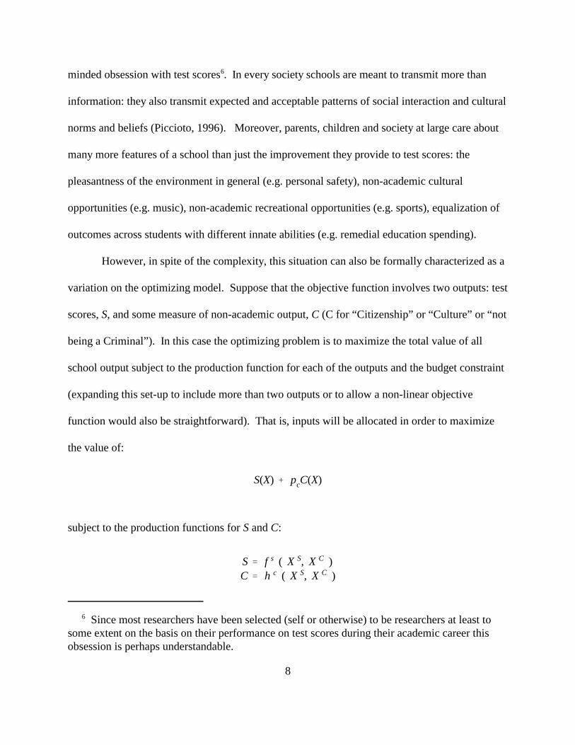
However, in spite of the complexity, this situation can also be formally characterized as a

variation on the optimizing model. Suppose that the objective function involves two outputs: test

scores, S, and some measure of non-academic output, C (C for “Citizenship” or “Culture” or “not

being a Criminal”). In this case the optimizing problem is to maximize the total value of all

school output subject to the production function for each of the outputs and the budget constraint

(expanding this set-up to include more than two outputs or to allow a non-linear objective

function would also be straightforward). That is, inputs will be allocated in order to maximize

the value of:

subject to the production functions for S and C:

f Si

pi

�

f Sj

pj

� pc�h C

j

pj

�

h Ci

pi

, � i,j

To estimate and interpret the cost function as the dual of the production function requires7

the assumption of maximization (Jimenez, 1986, Jimenez and Paqueo, 1996, James, King andSuryadi, 1996).

9

(3)

and the budget constraint.

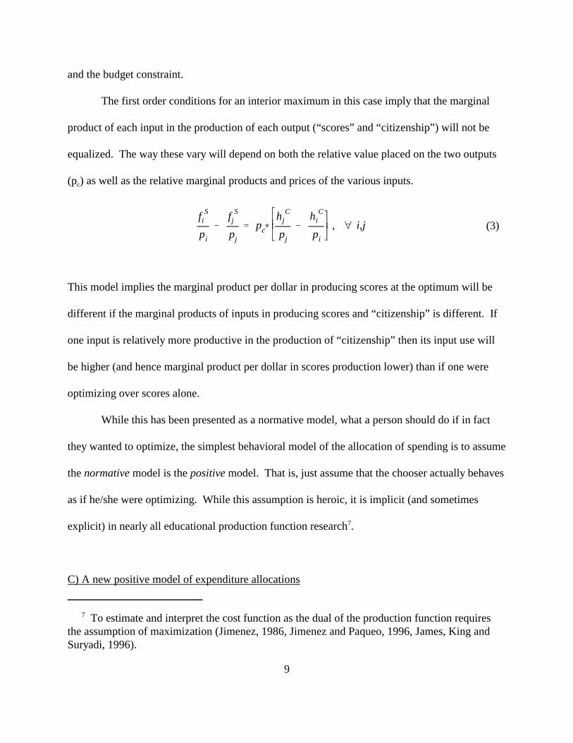
The first order conditions for an interior maximum in this case imply that the marginal

product of each input in the production of each output (“scores” and “citizenship”) will not be

equalized. The way these vary will depend on both the relative value placed on the two outputs

(p ) as well as the relative marginal products and prices of the various inputs. c

This model implies the marginal product per dollar in producing scores at the optimum will be

different if the marginal products of inputs in producing scores and “citizenship” is different. If

one input is relatively more productive in the production of “citizenship” then its input use will

be higher (and hence marginal product per dollar in scores production lower) than if one were

optimizing over scores alone.

While this has been presented as a normative model, what a person should do if in fact

they wanted to optimize, the simplest behavioral model of the allocation of spending is to assume

the normative model is the positive model. That is, just assume that the chooser actually behaves

as if he/she were optimizing. While this assumption is heroic, it is implicit (and sometimes

explicit) in nearly all educational production function research . 7

C) A new positive model of expenditure allocations

C(X) � (1��)�S(X) � ��T(X)

This is not referring to the direct effect teacher morale or satisfaction or compensation8

might have on output, as this is already embedded into the production function (so far have saidnothing about the structure of the production function).

10

Very few people would accept the optimizing model as a complete or accurate description

and in fact the production function has had very little empirical success in explaining school

performance. However, since the intuitive foundations are so clean and attractive the difficulty

in rejecting the optimizing model is proposing a specific, concrete, alternative against which to

judge it. Therefore, before turning to the empirical evidence we propose a very simple

alternative model, which embeds the optimizing models as a special case.

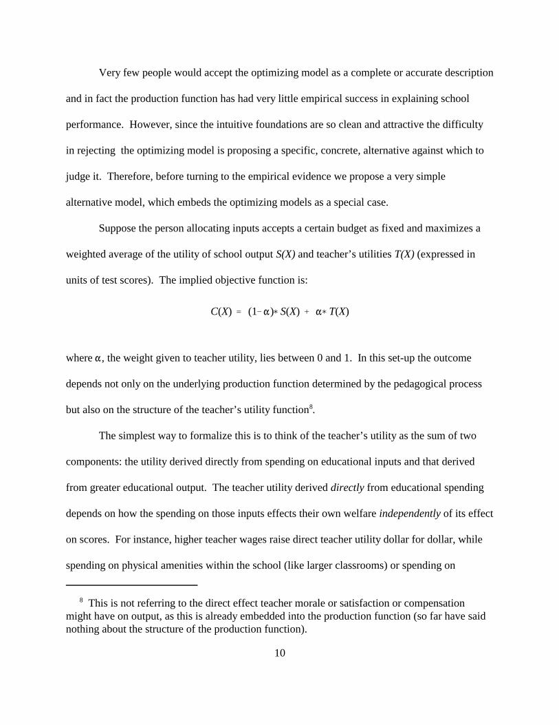
Suppose the person allocating inputs accepts a certain budget as fixed and maximizes a

weighted average of the utility of school output S(X) and teacher’s utilities T(X) (expressed in

units of test scores). The implied objective function is:

where �, the weight given to teacher utility, lies between 0 and 1. In this set-up the outcome

depends not only on the underlying production function determined by the pedagogical process

but also on the structure of the teacher’s utility function . 8

The simplest way to formalize this is to think of the teacher’s utility as the sum of two

components: the utility derived directly from spending on educational inputs and that derived

from greater educational output. The teacher utility derived directly from educational spending

depends on how the spending on those inputs effects their own welfare independently of its effect

on scores. For instance, higher teacher wages raise direct teacher utility dollar for dollar, while

spending on physical amenities within the school (like larger classrooms) or spending on

T(X) � (1��)�U(��X) � (�)�S(X)

Maximize [ (1��) � ��� ]�f S(X) � ��(1��) �U(��X)

s.t. p �X � B

11

reducing workload (like smaller classes) would raise teacher welfare, but not by the equivalent of

an unrestricted dollar given to the teacher, and spending on items like books or desks for students

would have zero (or near zero) impact on direct utility. Teacher utility also depends, through

altruism or professionalism, directly on educational output. The total teacher utility function is:

where U() is the direct utility derived from inputs, � is a vector which gives a weight to each of

the inputs (weights which lie between 0 and 1). The individual � ’s for each input are the relativei

prices, in that they are the teacher’s willingness to pay for an additional dollar of spending on

input i relative to their willingness to pay for a dollar of salary and hence are pure numbers. The

“professionalism” parameter, �, also lies between 0 and 1.

Now the optimization problem in allocating spending to raise this weighted average of

teacher utility and test scores is:

While this model is in many ways a modest generalization of the previous model, it has very

different predictions about the allocation of expenditures. In particular, the ratios of the marginal

educational output per dollar of input will not be equalized across inputs. Instead of implying the

difference in marginal utility per dollar of inputs will be zero, as in the simple optimizing model,

the first order conditions of this model imply:

f Si

pi

�

f Sj

pj

�

�(1��)(1��) � ��

� Ux� [�j

pj

�

�i

pi

]

12

(4)

That is, as long as the weight given to teacher utility is not exactly zero (���) and the degree of

professionalism of teachers is not sufficiently high that they are completely selfless (�<1) then

marginal products per dollar will not be equalized. The more directly an input enters teacher

utility (a higher � ) the lower the marginal product per dollar of that input in producing educationi

will be, relative to another input at the optimum.

The intuition is clear: since the chooser of inputs cares directly about teacher utility this

will lead to a higher level of spending on inputs that teachers care about and because marginal

products are declining this higher level of utilization will lead to a lower marginal product per

dollar of that input. Conversely, those inputs that do not enter directly into teacher’s utility will

have higher marginal product per dollar because their level of use will be lower than under pure

optimizing. In this model, the marginal product per dollar of inputs that teachers value directly

(e.g. wages) will be smaller than the marginal product per dollar of inputs which teachers value

indirectly (e.g. smaller class sizes, better physical facilities) which, in turn, will be smaller than

those that teachers value only because of their effect on achievement (e.g. books).

The combinations of books and teachers that produce constant amounts of educational9

output.

13

Figure 1 illustrates the case with only two hypothetical inputs, call them “books” and

“wages.” The educational output optimizing choice would be to choose point A, where the

educational output isoquant , whose slope is the relative marginal product of books to teachers, is9

tangent to the budget line, whose slope is the relative price of books to teachers. At this point the

conditions for an (interior) maximum are reached.

Adding teacher’s utility directly to the chooser’s objectives implies that the isoquants of

this new objective function are steeper than those of the educational output only isoquant. This

Several recent papers have examined whether teachers are “overpaid” by comparing wages10

or incomes of teachers either with cross-national norms (Cox-Edwards, 1989, Carnoy andWelmond, 1996) or with wages of other individuals, controlling for individual characteristics,like age and education (e.g Psacharopoulos, 1987). To see why this literature is distinct, imaginethat receiving a teaching position was like a sinecure, for which the teacher received a fixedannual payment completely independent of performance, and imagine that therefore teachers didno teaching at all. In this hypothetical case the “wages” of teachers could be arbitrarily low andyet the ratio of marginal product of teacher to non-teacher expenditures still be quite high.

14

implies the new equilibrium for a given budget will involve more teacher and less book spending

(point B). This higher level of spending reduces the marginal product per dollar of teachers

(illustrated in the southeast quadrant) and increases the marginal product per dollar of books

(illustrated in the northwest quadrant), which were equal when the objective function included

only achievement. When teacher’s utility is added to the objective function, relatively less is

spent on “books” and relatively more is spent on “wages” so that the marginal product per dollar

of “books” is high relative to the marginal product per dollar of “wages.”

Before moving to the evidence, let us make two points. First, our alternative model is

not derived from first principles. At this stage we do not propose a particular reason why teacher

utility is present in the objective function: it could be the result of patronage maximization of

politicians, it could be the result of budget maximizing bureacrats. Therefore “�” is our

alternative model does not necessarily represent “teacher power” or the benefits to individual

teachers, but rather represents a possible outcome from a broad class of models from which could

this weight on teacher inputs could be be derived. We return to this point in Section III below

when we discuss policy.

In particular, we are not arguing that teachers are individually overpaid, a point we return

to in the final section . Nor are we arguing “too much” is spent on education as we do not10

Much of this literature relevant to developing countries has been done at, or for, the World11

Bank (Lockheed and Hanushek, 1988, Hanushek, 1995, Harbison and Hanushek, 1992, Glewwe,1996, Hanushek and Lavy, 1994, Khandker, Lavy, and Filmer, 1994, Tan, Lane and Coustere,1996, World Bank, 1995).

15

model the determination of the overall budget for education, which could be low. In many cases

spending on teachers (or the budget overall) is “too low” in any absolute sense, even if teacher

spending is “too high” relative to the productivity of other inputs.

II) Our reading of the evidence

How do the predictions of the two classes of models, output maximizing and teacher

influence, fare when faced with the evidence? There is an enormous literature examining the

relationship between the level and composition of educational spending and the output of the

educational process . We review three types of evidence in the literature: studies of cost11

effectiveness, education production function estimates, and direct evidence from differences in

parental control within educational systems. Together this evidence overwhelmingly rejects all

three variants of the educational output optimizing models (simple, uncertainty, and multiple

output) in favor of a model which incorporates teacher utility into decision making. To preview

the results, the failure of the equalization of marginal product per dollar rejects simple

optimizing. The systematic pattern of that rejection across inputs: that educator related inputs

tend to be overused relative to non-teaching outputs, rejects the uncertainty (and we believe,

multiple output) models. The comparisons between public and private schools, or schools with

more or less parental control, or comparisons of outcomes with different teacher unions,

definitively reject all three educational output optimizing models.

Unfortunately, it is impossible to recover comparisons of the marginal versus average12

distinction from the existing empirical literature.

16

A) Empirical estimates of the cost effectiveness of various inputs

The key hypothesis to test the simple optimizing versus our model is whether the

marginal products per dollar of all educational inputs are equalized. However, studies only rarely

go on from estimating the marginal products in physical terms (e.g. the effect of class size on test

scores) to calculating the educational gain per dollar spent, typically called “cost effectiveness”,

which is the best guess at the marginal product per dollar of spending of different inputs at the

observed allocations . 12

Table 1 reports the cost effectiveness estimates derived from a large scale evaluation of

an education project in Northeast Brazil (Harbison and Hanushek, 1992). These estimates line

up exactly as we would have expected if there is a substantial amount of teacher influence. The

cost effectiveness of teacher salaries (normalized to 1) is by far the lowest. Material inputs

which provide amenities to the school and teachers, such as teacher tables, toilets, bookcases,

have a cost effectiveness on average 7.7 times larger than teacher salaries. Instructional

materials, which provide benefits to teachers only insofar as they increase scores, have cost

effectiveness ratios between 17 and 34 times as large as the impact of additional spending on

teacher salary increases. The prediction of the simple optimizing model, that cost effectiveness

is equalized, is wrong by at least an order of magnitude.

17

Table 1: Ratio of test score gain per dollar in Portuguese and Mathematics for variousinputs relative to teacher salary (=1), average estimates from Northeast Brazil

Grand average(years,

subjects,grades) Portuguese Mathematics Portuguese Mathematics

Second grade (Average Fourth grade (Average1981,83,85) 1983,85)

Material inputs

Textbook usage 17.7 33.9 22.7 14.5 0.0

Writing materials 34.9 11.8 13.8 58.8 55.3

Software* 19.4 19.4 13.4 24.5 20.3

Infrastructure inputs

Hardware* 7.7 3.4 3.5 16.0 8.1

Alternative teacher education strategies

Curso de Qualificacao 5.0 1.2 2.5 5.0 11.3

Logos 8.3 8.3 6.8 13.5 4.6

4 years primary school 6.7 8.5 13.2 0.0 5.3

3 years secondary school 1.9 2.5 3.9 0.0 1.5

Teacher salary

Teacher salary 1.0 1.0 1.0 1.0 1.0

* Hardware: water, bookcase, teacher table, pupil chair, pupil desk, two classrooms, large room, director's room,kitchen, toilet, store cupboard Software: writing material, chalk, notebook, pencil, eraser, crayons, textbook usage

Source: Derived from Harbison and Hanushek (1992), Table 6-2

Table 2 provides similar estimates from a large scale study of student achievement in

eight states in India (World Bank, 1996a). The cost effectiveness of increasing teacher salaries is

again normalized to 1. The cost effectiveness of spending on improving physical facilities is

higher than that of teacher salaries (1.2 times higher), however that for increasing just classroom

size is between 1.7 and 4 times higher. The cost effectiveness of spending on instructional inputs

is between 4 and 14 times higher than that of increasing teacher salaries. Again the actual ratio

between the marginal product per dollar of salary inputs and instructional materials is different

from the level predicted by optimizing model by more than an order of magnitude, 14 to 1.

Since this study did not report cost data for school resources, we used data from World13

Bank (1996a) to calculate these ratios.

18

Table 2: Test score gain per rupee for various inputs relative to teacher salary (=1), averageacross low-literacy districts in eight states of India, 1993

Instructional materials

Complete package of instructional materials and aids 14.0

Coverage under Operation Blackboard, equipment only 4.0

Physical facilities

Full package of facilities 1.2

One additional square foot per student

Cost based on school construction in Uttar Pradesh 4.3

Cost based on DPEP average 1.7

Teacher Quality

Increasing average teacher salary by Rs. 100 per month per school 1.0

Opportunity to learn

Reducing the pupil teacher ratio by one 0.1

Adding one additional school day per academic year 1.0

Adding one additional teaching hour per academic year 0.6

Adding one additional hour of language instruction per academic week 29.0

Source: World Bank (1996a) Annex F

What is somewhat puzzling is that class size reductions are even less effective than

teacher salaries. However both of these results are consistent with recent estimates by Kingdon

(1996) using sample survey data for students from 30 schools in urban Uttar Pradesh, who finds

that if the cost effectiveness of teacher salary is normalized to 1, the cost effectiveness of class

size reductions is .029 but the cost effectiveness of increasing school physical resources is 3.2 . 13

B) Education production function estimates

Do these few cost effectiveness studies represent the typical case across a variety of

conditions? While there are few studies that calculate cost effectiveness for different types of

We include only inputs reported in the surveys of the literature that were subject to 10 or14

more studies.

This ranking is problematic as the interpretation of a coefficient depends critically the other15

variables included in the regression. For instance, some regressions include “instructional time,”if teacher salaries are included in the same regression then more time for the same salary wouldbe a real wage reduction which teachers should oppose so that the marginal product should bevery high. If teacher salaries are not included then its sign is ambiguous. Similarly, thecoefficients on “teacher training” or “teacher education” all depend on what else is included inthe regression.

19

inputs, there are numerous studies which relate student achievement to school characteristics,

such as inputs, while controlling for student’s background characteristics (e.g. parental income,

education) and there have been several prominent reviews of this literature. These reviews face

enormous difficulties in summarizing the empirical results of the different studies as the

estimated coefficients, which are reported in physical quantity units, (e.g. test scores gain per

square foot) are not directly comparable either across inputs or across studies. Therefore the

reviews summarize only whether the effect was estimated to be positive or negative and whether

it was statistically significant (although some do attempt to report “effect sizes” which, at least

normalizes the test scores to standard deviation, Lockheed and Haunshek 1988).

Confirmation percentage evidence. Holding these problems firmly in mind, there are two

ways we can bring the enormous educational production function literature to bear on our

competing positive models. First, we can compare the “confirmation percentage” of various

inputs, that is the frequency with which the variable is found to be statistically significant of the

expected sign sorted by our conjectures as to which inputs are of most and which of least direct

importance to teachers . In the most recent of these compendia, Fuller and Clarke (1994)14,15

summarized in Table 3, there is a markedly higher confirmation ratio for the inputs, like facilities

20

and instrumental materials, which are less likely to appear directly in teacher’s utility (two other

reviews, Harbison and Hanushek, 1992 and Velez, Schiefelbein and Valenzuela, 1993 report

similar results and are included as appendix 1).

In Table 3 “teacher’s salary” has a confirmation rate of 36 percent for primary and 18

percent for secondary schools, the confirmation rates of teacher-pupil ratio are 35 and 9 percent

respectively. In contrast, the presence of a school library has a confirmation rate of 89 percent

and the availability of textbooks a confirmation rate of 73 percent for primary and 54 percent for

secondary schools. Interestingly, a review of 43 studies (appendix table A.2) found that only 4 of

those found a significant and positive relationship between “teacher satisfaction” and student

achievement.

Table 3: Confirmation percentages of various educational inputs sorted by direct importance to teacher utility.

Number of studies significant relation PercentagePositive and Confirmation

Primary Schools:Teacher's salary level 11 4 36.4

School teacher pupil ratio 26 9 34.6

Teacher's years of schooling 18 9 50.0

Teacher's experience 23 13 56.5

Class instructional time 17 15 88.2

Class frequency of homework 11 9 81.8

School library 18 16 88.9

School textbooks 26 19 73.1

Secondary schoolsTeacher's salary level 11 2 18.2

School teacher pupil ratio 22 2 9.1

Teacher's experience 12 1 8.3

Class instructional time 16 12 75.0

School textbooks 13 7 53.8

Source: Fuller and Clarke (1994)

21

If marginal product per dollar were equalized, there is no compelling reason to believe

that the confirmation ratios would not have been roughly equal across inputs. While this evidence

is far from airtight, as it is possible the differences in precision could have affected the pattern of

statistical significance, the most straightforward way to read this evidence is that studies that use

non-experimental data systematically evaluate the marginal product of inputs at points that are

not education output maximizing. The results suggest that at the input spending allocations

typically observed in non-experimental data in which these allocations are the result of choice,

the marginal product of inputs is lower for those inputs more highly valued by teachers and hence

they are more likely to be statistically insignificant.

The second way these production function studies could be brought to bear on the

competing hypothesis is to calculate estimates of the marginal product per dollar from the results.

Unfortunately, after scouring this literature we found very few studies that report the necessary

information, principally because they lack data on the relative costs of various inputs. Even

among those that do report some estimates of cost effectiveness, standard practice is to calculate

cost effectiveness only for those estimates that happen to be statistically significant (and in the

right direction). Table 4 reports the educational production function estimates by Tan, Lane, and

Cousternane (1996) for which they calculate cost effectiveness only for those few inputs,

particularly workbooks and furniture, that were statistically significant. They do not however

compare cost effectiveness per dollar with other inputs, such as reductions in class size. Using

their estimates and information about teacher salaries and class sizes from other sources we

calculate that at the estimates they report, providing workbooks was 800 to 1600 times, and

providing furniture 700 to 1200 times, more cost effective than reducing class sizes. One might

22

object we are using a statistically insignificant, and hence potentially imprecise, estimate on class

size, but even if we add two standard deviations to the point estimate for class size (that is

increase it to the upper range of a 95 percent confidence interval) the impact of workbooks or

furniture was 100 times larger than of reducing class size. This is still two orders of magnitude

larger than the ratio predicted by an optimizing model.

Table 4: Calculating relative cost effectiveness of teacher to non-teacherinputs while taking precision of estimation into account.

Input: Subject: Ratio of cost effectiveness of inputs to increasing classsize:

At point estimates of all Adding two std. dev. tovariables class size point estimate

FurnitureMath 689 90

Filipino 1243 113

WorkbooksMath 842 110

Filipino 1592 145

Notes: In order to calculate the cost of decreasing class size, we use the fact that averageteacher salary is 2.5 times GNP per capita (World Bank, 1996b) and assume that eachteacher teaches an average of two classes, and that the average class size is 40.19 asreported in Tan and others (1996).

Since most investigators begin with a presumption that the inputs into education are

reasonably well known, presumably the key critical question that estimation of a production

function could help resolve is whether reallocating inputs given a fixed budget could improve

performance. Reporting only estimates of the production function with no estimates of costs is

not even relevant to that question. The distressingly common practice of reporting the

production function estimates of known educational inputs in quantity units (e.g. class size) text

By stipulating known inputs we distinguish studies of pedagogical innovations such as 16

radio instruction, computer assisted learning, alternative teaching strategies, etc., where thequestion of zero marginal product over all ranges is actually a useful null hypothesis.

One huge problem with reporting only signs and statistical significance concerns statistical17

power. Failing to reject that a particular coefficient is zero could result either because theestimated impact was small or because the impact was large, but very imprecisely estimated. Ifthe effect of some inputs is estimated with greater precision then these will tend to be more“significant” even if they are empirically smaller. Moreover, there is no necessary connectionbetween the precision of the estimates in quantity units and cost per unit so one may “fail toreject” the test of zero impact for some inputs which have extremely high cost effectivenesswhile finding statistically “significant” other inputs with low cost effectiveness.

23

books, physical facilities and their statistical significance without comparative information on

costs is nearly devoid of policy interest . 16

This also raises a problem for the “meta-analysis” approach to creating statistical

significance, in that it ignores the actual underlying policy question and the asymmetry in what

the two sides of the “money matters” debate are asserting. That is, if the impact of teacher inputs

(e.g. salaries, class size) is not demonstrably different from zero then it is also not optimal, in the

sense of equalized marginal products. However, showing only that teacher inputs, or budgetary

inputs generally, have some impact (which can be done with meta-analysis Hedges, Laine and

Greenwald, 1994) does not address the question of whether those levels of inputs are optimal or

whether reallocations in expenditures could increase output. Moreover, calculating cost

effectiveness for only those estimates that are statistically significant confuses the magnitude

with the precision of the estimate . 17

One intriguing aspect of using a normative optimizing production function model as a

positive descriptive model of behavior in an empirical study is that these assumptions self-

referentially predict the impact of the study itself. If educational policy makers are assumed to be

There raises another, borderline ironic, sub-text to the econometric production function18

estimates. In order for the estimates from non-experimental data to correctly identify anunderlying production function there needs to be some mechanism that causes different choicesof input mix other than shifts in the production function itself. If differences in input use acrossthe levels of the data (e.g. districts, schools, etc.) are due to differences in teacher’s utility weight(�) in the objective function across policy makers then this implies the empirical estimates arecorrectly identifying the production function. However, while these makes the estimatestechnically correct it also makes them irrelevant for policy.

24

attempting to optimize, then choosing too much teacher expenditure relative to spending on

physical facility, equipment or books could only have been because of a mistaken belief about

the “true” production function. But then the behavioral model predicts that the study itself (if

believed) should cause a reallocation of resources towards the more productive resources as the

new information fixes the previous mistake. Has this (implicit) prediction of output maximizing

models been confirmed?

As we presented in the section above, the weight of international evidence of too little

spending on some inputs has always been impressive, and has been accumulating over time.

Fuller and Clarke, in their 1994 review, point out that while there were 37 new studies since the

review of the evidence in 1986 (Fuller, 1986), the new studies mostly confirmed previous

patterns, particularly the relatively greater importance of books and instructional materials than

class size and teacher inputs (Fuller and Clarke 1994). However, while recent data are very

difficult to come by, the share of educational expenditures devoted has, if anything, shifted

towards an even greater share of teacher compensation (although this may be due to a fiscal

contraction.) We know of none, and conjecture it would be difficult to document a single

instance in which an empirical study, or even a series of studies, actually affected the distribution

of expenditures . In contrast, a model that explains the existing spending allocation as the result18

The specifications in this literature use quite simple assumptions about the production19

function, usually that output is linear or log-linear in inputs. In particular this rules outinteractive effects between inputs which are potentially important. Also, the analyses reportedabove may suffer from the fact that the specifications are not identical across the various resultsreported. Even so, World Bank (1996a) reports results from estimating the exact same functionalform of an educational production function in low literacy districts in eight Indian states, for twodifferent educational outcomes. The results clearly show that the significance (and sign) of theeffects of the inputs vary widely across the different states even for exactly the samespecification.

25

of a political process implies that studies of the products of various inputs may, but probably will

not, influence spending which will require changing the incentives of decision makers

(summarized as “�” in our simple set-up).

Caveats about the educational production function literature. We should not overstate

our case as to the reliability of the educational production function literature in supporting any

hypothesis. Many of the studies find nothing to be statistically significant and often find perverse

patterns in the point estimates (for example negative signs on inputs like teachers or books).

Moreover, even when the estimates of the individual production function coefficients are

reasonable, school inputs typically have very small explanatory power. There are several

additional econometric difficulties with the literature and we should at least mention four:

simplistic and differing specifications , multi-collinearity, insufficient variation in input use, and19

different sensitivities among inputs.

One point on the latter two concerns. Suppose that there were a number of potential non-

teaching inputs with high, but steeply declining marginal products (like algebra books). A

perfectly random allocation of resources among these non-teaching inputs would produce a

pattern of some very large and some small estimated marginal products with the high

productivity of some of these factors due to the very low utilization. Different inputs might have

Using the results of World Bank (1996a) we perform a crude regression of the significance20

of the parameter estimate on the mean and standard deviation of the input. The results suggestthat for score on reading test the degree of significance of the effect of an input is significantlynegatively related to the mean value of the input. For the score on the math test, the estimatedmagnitude of the effect is significantly positively related to its standard deviation.

26

different amounts of variation in use . This pattern suggests that there are inputs for which the20

marginal product is very high at low levels but declines very rapidly. In this case one would

expect to see a very high marginal product for that input, but also observe that the input was

rarely in range of low use, and hence the empirical finding is of limited usefulness. For instance,

Glewwe (1996) conducts a study of the determinants of school quality in Ghana using a large

scale data set and the only statistically significant school level effects on math and reading test

scores are from the fraction of classrooms that have blackboards, and the fraction of classrooms

that cannot be used when it rains. However, even in Ghana, 90 percent of schools have

blackboards and only 15 percent of middle schools have leaking classrooms.

C) Direct evidence

The 10 to 100 fold divergences in marginal product per dollar across inputs, and that

these are in a consistent pattern across inputs, rule out both the simple and uncertainty optimizing

models. However, one could still return to the multiple output model and conjecture that the

observed pattern of marginal products in producing scores corresponds to the inverse pattern in

the marginal products in producing some other output. In this section we first say why we think

this objection is unfounded, and then show additional evidence that bears directly on the

difference between the multiple schooling output and our model, and which leans in favor of a

positive model with teacher influence.

Card and Krueger in various papers (e.g. Card and Krueger, 1996) have shown that budgets21

are related to subsequent wages of workers, but this evidence is not entirely relevant, for tworeasons. First, their studies are of aggregate budgets and do not address the question of relativemarginal products of various inputs. Second, their studies are consistent with wages being abetter measure of achievement than multiple choice tests without invoking any additionalassumptions that something besides achievement (e.g. “worker docility”) being produced byschooling.

27

There are three reasons the multiple output model is theoretically and empirically

inadequate. First, it appeals to variables that are either unobserved or unobservable, which

makes the model non-falsifiable. Someone with an interest in rejecting a positive model of

expenditures with teacher influence could always assert that the patterns of the marginal product

of inputs for the unobserved component of educational output (e.g. citizenship) are exactly what

they would have to be in order to rationalize the observed outcomes. Because the output is

unobservable they could make this assertion without fear of contradiction (or confirmation).

Second, related to the first, there is little or no empirical evidence of the effect of various

educational inputs on anything other than achievement . Third, it is hard to understand21

intuitively how a multiple output model could explain the existing empirical patterns, for

instance of teacher salary versus class size or physical facilities versus instructional materials. In

order for an appeal to multiple outputs to be satisfying, one would have to explain why is it that

the unobservable output of education requires enormously higher teacher salaries, more teachers,

but less physical facilities and less instructional materials than the observable output.

Parental versus educator power: Local and parental contributions, private schools and

unions. Fortunately, there is a source of direct evidence which is able to distinguish the multiple

output from the teacher influence models. As pointed out above, if the chooser is attempting to

optimize then new information about the production function should change inputs and

28

outcomes. In this section we argue that the converse is also true: if the optimizing model were

really correct then one should not see patterns of input use and outcomes respond to different

degrees of incentives. Greater local financing or control of schools, differing degrees of

competition, or differing amounts of union power should not affect technical efficiency. But the

evidence suggests that these factors do have an important effect both on the allocation of

expenditures and the efficacy of outcomes. The following section discusses three sources of

evidence relating to various sources of differences in parental power: the degree of local control,

teacher unions, and private schools.

Local and parental contributions. A first source of evidence is the impact of direct

parental participation and contributions. Modest amounts of direct contributions of parents

should have large effects on performance only to the extent that some inputs (infrastructure,

equipment, instructional materials) are so dramatically under-funded by the publicly allocated

budget that their marginal products per dollar are very high. If marginal products were equalized

(even according to an optimizing model with multiple outputs) then the relatively small

contributions should only have a proportionately small effect. Evidence of substantial impact by

parent’s groups, or of local control, or of the proportion of resources from local sources is itself a

sign of a failure to maximize outputs in the overall system of expenditure allocation.

Jimenez and Paqueo (1996) using data from the Philippines find that schools with a small

component of local financing (under 5 percent) are incredibly less productive than schools with

even a small share of public financing: their achievement score per dollar is only a third as high.

More importantly, the cost savings that produce this greater cost effectiveness come

Both of these papers use econometric estimation of the dual, that is, cost per student22

controlling for quality, rather than estimate a production function. However, their results onlocal financing indicate that the primal problem is not maximization of output subject to a budgetconstraint, but rather some more complicated objective function involving teacher utility of thetype we explore here.

29

disproportionately from personnel whose cost per student is 52 percent lower, with much smaller

cost savings for other inputs (Table 5).

Table 5: Relative cost effectiveness and expenditures composition of locally versusnon-locally financed schools

Proportion of funds from local sources:Percentage difference <5% > 25%

Overall score 42.46 48.25 13.6%

Total expenditures 675 265 -60.7%

Achievement score per 0.06 0.18 189.1%peso

Cost per student (Philippines pesos)

Personnel 469 226 -51.8%

Maintenance and 42 35 -16.5%operating

Textbooks 7 5 -26.6%

Source: Adapted from Jimenez and Paqueo (1996), table 1.

Similarly, James, King and Suryadi (1996) find that even controlling for whether schools

are public or private, a greater share of funds that are locally raised compared to centrally

allocated increases significantly educational output (in their model, decreases cost for a given

output) . 22

Many countries have adopted locally run community schools as a mechanism to

accommodate the demand for schooling in remote and rural areas that are not reached by the

“official” school system. One common feature of these schools is that the teachers are hired by

the local community and are not education ministry employees and are not subject to the usual

30

qualification requirements. While there is little direct evaluation of these schools that can

compare costs and outcomes, the existing evidence suggests that community managed schools

user fewer “teacher wage” inputs and achieve essentially the same or better academic results.

Results on local financing and the experience with community schools are consistent with

more centrally controlled resources being allocated by an optimizer with a high concern for

teacher welfare (high �) principally to teacher inputs, while locally raised funds being subject to

a greater degree of parental control and hence high concern for educational output (low �) and

are allocated principally to non-wage inputs with high marginal product.

Private schools. The evidence from five developing countries marshaled by Jimenez and

Lockheed (1995) shows that, even controlling for selection effects, private schools are

significantly more cost effective than public schools. This fact alone is inconsistent with the

simple or uncertainty optimizing model of the allocation of the public budget. However, it is

possible that the improvement in efficiency is due to pure X-inefficiency of public schools, that is

public and private schools do not differ in the allocation of inputs but simply that private schools

are uniformly more productive for all inputs. An alternative explanation, consistent with a model

of teacher influence, is that private schools, if they are more subject to competition for

enrollments, are more directly controlled by parents. By being more subject to parental pressure

and less susceptible to teacher power the managers of private schools (or private school systems)

will have a lower “ �” than public school system managers and these differences in parental

control should produce both higher effectiveness of the budget overall and also different ratios of

inputs. Importantly, since evidence from private schools is based on parental willingness to pay

for schooling it does not depend on test scores as the measure, as it incorporates parent’s

31

concerns about the all schooling outputs. If the observed difference in marginal products per

dollar of inputs were the result of optimizing over multiple outputs and public and private

schools were optimizing over the same set of outputs, then one should not observe systematic

differences across the marginal products of various inputs between private and public schools.

Fortunately there is a recent study that provides almost exactly this test. Alderman,

Orazem and Paterno (1996) examine how the characteristics of schools (like instructional

expenditure per student and class sizes) affect parental decisions between private and public

schools in Lahore, Pakistan, an urban area where 58 percent of students are enrolled in private

schools even though private school fees are 5 times higher. They find, controlling for class sizes

and instructional expenditures, that achievement scores were 60 percent higher in private

schools.

Since school level instructional expenditure represents almost entirely teacher salaries we

can compare how much parents are willing to pay to increase salaries versus decrease class sizes.

As shown in table 6, parental willingness to pay to increase salaries in the private sector was

almost six times larger than in the public sector, suggesting that the marginal product of

additional teacher wages in terms of all parental valued outputs (not just scores) in the public

sector was already quite low. Conversely, class sizes were so high in the public sector that

parents were willing to pay substantial amounts to reduce them, and were substantially more

willing to pay for class size reductions than wage increases, the opposite of the private sector.

Since we believe that there are qualitative differences between the US case and that in23

developing countries, we are reluctant to use any evidence at all from the US, as this raises awhole host of US specific issues. However, the evidence provided here is too unique and toodirectly related to the question at hand to pass up.

32

Table 6: Parental willingness to pay for teacher salary increases versus class sizereductions in private and public schools in Pakistan.

Private school Public School Ratio Private topublic

Expenditures per teacher (rupees per month) 7711 8406 .92

Parental willingness to pay to increase 40.4 7.05 5.7instructional expenditure per pupil (a proxy forteacher salaries of Rp 200)

Average class size 25.2 42.5 .59

Parental willingness to pay to decrease class size -35.7 7.10 --by 10 students

Ratio of willingness to pay an additional rupee to � .47 --teacher salaries versus class size reductions

Notes: Adapted from tables 2 and 5, using willingness to pay of parents with monthly household income of Rp.3000 (Alderman, Ozarem, and Paterno, 1996).

Unions. Caroline Minter-Hoxby has two recent pieces of research, which although they

are on the US and not developing countries, are relevant to the issue at hand . In one (1994) she23

shows that the larger the number of school districts within a given metropolitan area the better

the performance of the schools. She argues this is evidence that greater competition among

public school districts substitutes for school choice and increases performance. Another paper

(1996) shows that even after controlling for the endogeneity of unionization, school districts that

are unionized are less effective than the non-union school districts. She shows that in districts

with unions, spending on schools is higher but a larger proportion goes to teachers.

The two best arguments against this are the meta-analysis of studies in the US (Hedges,24

Laine and Greenwald, 1994) and the studies of the impact on subsequent wages of budgetaryresources while in school (Card and Krueger, 1996), also done exclusively in the US. Both ofthese are reasonably convincing that there is some, but small, connection between expendituresand outcomes, which of course under a positive maximizing model must have been the case. Butneither of these methods speak to the question of whether a different budgetary allocation couldhave had a larger impact.

33

III) Implications of a positive theory for educational policy

We have shown that the educational output optimizing model of expenditure allocation,

in all its variants is inconsistent with the evidence and that a simple model in which teacher

utility receives direct concern in expenditure choices is consistent with the stylized facts. Having

a positive model of educational spending is important for the analysis of policy options. As

mentioned in the introduction, there are two kinds of educational policies currently proposed:

more of the same (higher enrollments, higher expenditures, better teacher training, etc.) and

fundamental reform of incentives (decentralization, community involvement, school choice,

etc.). Guidance on the choice between these requires modeling the underlying public sector

decision and control mechanisms as fundamental reforms are about changing the incentives

within the sector.

A) More budget versus reform

As mentioned above, one of the puzzles in the literature on educational production

functions is that it is often difficult to demonstrate a positive impact of increased spending on

educational outcomes . The literature is criticized precisely because the results seem so24

implausible to educators and educated alike: of course "money matters" and on some level

There has been a vociferous debate in the US around the question “does money matter?” 25

In this political debate the rejoinder "the only ones who say resources do not matter have theirchildren in schools with adequate resources" carries a good deal of common sense appeal.

Differences in the relative weight of teachers also happen over time within a given26

jurisdiction as across jurisdictions. For instance, in Paraguay after the end of a long period ofdictatorship teacher wages more than tripled in a six year period, with an almost complete lack ofcomplementary reforms either in the school system or even in the structure of teacher pay. Giventhe total lack of objective comparable testing it is impossible to say for sure, but many doubt thisincrease led to commensurate increases in student performance.

34

everyone knows that . But the implication of our positive model is that while “money matters”25

to educational outcomes, money also matters to those who receive it as income and that

“mattering” will have implications for publicly determined outcomes, like the allocation of

expenditures.

Budgets and educational outcomes when objectives differ. If non-experimental data are

taken from jurisdictions (or time periods within the same jurisdiction) that differ in either the

degree of educational output concern (1-�) or in the degree of professionalism (�) of the teachers

then equal budgets could produce very unequal outcomes due to the allocation across inputs . 26

For any given level of �, higher budgets lead to better outcomes (the sense in which money

matters). But a higher � implies worse outcomes for any given budget. Any estimation of the

relationship between expenditures and budgets from non-experimental data that differ in � which

do not control for these differences can produce any relationship at all: positive, zero, or

negative. For instance, Hanushek and Kim (1996) estimate the relationship between the

internationally comparable test scores of achievement in math and science derived from the

various IEA and IEAP studies and expenditures. They find that both public expenditure per

student and the ratio of total educational expenditure to GDP are significantly negatively related

Differences in misallocation relative to the optimum is only one possible explanation of the27

empirically small impacts of budgets on outcomes. The other is that educators are systematicallyignorant of the true pedagogical function, and ideological blinders, not self-interest preventsthem from acknowledging the truth. This is essentially the controversial argument E.D. Hirsch(1996) makes about schooling in the US. In this case more resources do not produce greateroutput because of ignorance about the production function.

35

to achievement. While this obviously cannot represent the impact of the relaxation of the budget

constraint, if higher � values are associated with higher budgets then the data across jurisdictions

on budgets and outcomes could show a negative relationship, as in figure 2 with a line fitted to

hypothetical outcomes A, B and C, even though for any given � a budget increase would improve

scores .27

Given that both budgets and their allocation matter, what should be the focus of

improving school performance? The answer that will be guaranteed vocal support is “increase

budgets” as this generates support among parents, the general public who have an interest in

promoting better education, and teachers (for both professional and self-interested reasons).

36

However, if the existing allocation of inputs is not optimal, school performance can also be

improved by a reallocation of expenditures with no increases in the overall budget. These

proposals will tend to split the above coalition and pit educators against all others. Which type of

reform will be the most effective if implemented? The answer is, not surprisingly (and even

reassuringly), it all depends. If the budget is high and � is high then fundamental reforms are

more pressing. If on the other hand the budget is low and � is low then budgetary reform should

receive priority.

To say more, we can make specific (and very limiting) assumptions about the functional

forms of the production function and teacher utility (Cobb-Douglas) and assume no teacher

professionalism. Under these assumptions we can solve explicitly for the relationship between

scores, budgets and �. In this case, the score improvement from budget increases approaches

infinity as the budget tends to zero and approaches zero as the budget tends to infinity for any

Both of these results are illustrative only as they follow quite mechanically from the Cobb-28

Douglas assumptions, which implies that each input is “essential” in the sense its marginalproduct goes to infinity as the level of input approaches zero.

37

given �. The incremental impact of changes in � on scores approaches zero as � goes to zero

and approaches infinity as it approaches one . As can be seen in figure 3, this situation implies28

that for any given level of the budget, B there is a critical level, �*, such that for all levels of �0

above �* the increment to changing � will have a greater impact than changing the budget.

Similarly, for any level of teacher power, � , there is some level of the budget low enough (B*)0

such that increasing the budget will have more impact on scores than changing teacher power.

B) Three possible models behind the model

The model we have specified is ad hoc, in that it is not derived from underlying behavior

by actors, and hence is more of a description of a class of models that might be derived from

different structural assumptions. That is, we have not articulated a complete model which

specifies which person or entity controls the allocation of spending (a school board? a

legislature? the ministry of education?) nor why exactly that person or entity cares directly about

teacher welfare. For many of our conclusions the exact model is not important. However, to

move to the predictions about outcomes of more specific reforms one needs to specify a more

complete model. There are three prototype models: principal-agent, teacher power, and

patronage, each of which has different implications for policy.

Principal-agent. In this model the decision maker can be either the parents themselves or

a manager that faithfully represents parent interests. The source of teacher weight in the

objective function is superior knowledge by teachers about the production function. In this case,

“People of the same trade seldom meet together, even for merriment and diversion, but the29

conversation ends in a conspiracy against the public, or in some contrivance to raise prices.”

38

teachers will systematically misrepresent the production function so as to lead the chooser of

budgets to choose greater spending on those inputs that teachers prefer. In this model, empirical

studies actually might have some impact by revealing the true production function. This

particular model predicts a systematic tendency of educators to resist quantitative evaluation of

their output, as this allows checking the reported production function against the actual.

Teacher power. The second possibility is that teachers as a group are powerful enough to

affect the allocation of education expenditures. In this case, there is a third party (e.g. minister of

education) or institution (e.g. legislature or school board) that controls budgetary allocations and

has to choose between pleasing a concentrated group of educators and a diffuse group of parents.

Given that on issues like teacher wages educators have a very clear and direct interest, they may

be more successful at organizing to influence public decisions than are parents. In this case, the

problem is not that parents are systematically under informed about the production function, but

that parents have greater difficulty overcoming the free rider problem inherent in collective

action than do teachers (Olson, 1965).

In our model greater teacher professionalism helps output. However, the mechanisms

that foster greater teacher professionalism are precisely those that tend to create greater teacher

power by making cooperation in lobbying easier. A common recommendation of education

professionals is to get teachers to work together, to share experience, give support, etc. However,

teachers are no different than any other group and Adam Smith’s adage applies .29

39

Patronage. Another possible model is that teachers are not particularly powerful but the

chooser of expenditures is powerful. Suppose that the Minister of Education can allocate all jobs

and each job creates a favor. In this case the chooser would want teacher salaries to be relatively

low (but a slight premium so that the job is a “favor”) but would want to maximize the

employment of teachers. In this case teachers would be poorly paid individually but there would

far too many teachers. This might explain those cases in which the marginal product of teacher

salary was greater than that of class size as the total wage bill to the chooser is more important

than the wage.

C) The analytical base for fundamental school reforms

A positive model of educational expenditures will also provide guidance to the actions or

reforms that are likely to improve outcomes. In particular, there are three commonly proposed

actions that are unlikely to lead to significant changes in performance: more research into the

technical pedagogical processes behind the production function, more school choice without true

competition, and greater parental involvement without control or choice.

Ignorance or incentives? Even though, as in all fields that involve human behavior, there

are enormous areas of ignorance, the fundamental problem is typically not teacher or technocrat

ignorance that could be resolved by more research. Our positive model implies several things

about education research. First, since some types of research are inimical to furthering certain

interests this implies that one should expect there to be relatively little research into cost

effectiveness of various inputs from educational production functions. The amount of ignorance

This point is not lost on legislators or policy makers. In Horn’s (1995) terminology the30

“enacting coalition” of interests have incentives to prevent future legislators or policy makersfrom undoing their agreement. In the US for instance, certain types of regulatory legislationexplicitly forbid the implementing agency from considering costs. During certain periodsDepartment of Agriculture economists were forbidden from doing any research on the economiclosses from existing agricultural policies. A recent example is the Clinton administration’srefusal to redo a study of the impact of welfare reform which had been influential in scuttlingearlier legislation (The Washinton Post, July 26, 1996).

Again, teachers are not alone in this as capital intensive innovations have always brought31

resistance from those with specific human capital. In fairness, labor intensive innovations havealso met staunch resistance, such as the persistent opposition to land reform from large landowners in Latin America (Binswanger et al, 1993).

40

is endogenous, and sometimes it pays to be ignorant . Second, only well disseminated and30

widely understood studies that foment deep public dissatisfaction with the schools would be

likely to change the incentives of the actors within the system and hence have any influence on

outcomes. Merely documenting the differences, as has been done in many times and many

places, will typically have no effect.

Finally, an implication similar to the lack of new studies in influencing expenditure

allocations is that educational innovations that are labor saving will be under adopted. That is,

when technological advance shifts the production function such that more of some other input

and less of teaching input is now optimal, one can expect to see resistance and see that the

adoption rate is very slow, or occurs without any labor saving . In almost complete ignorance,31

we would predict very slow and patchy adoption of innovations like rural radio based instruction,

shown almost twenty years ago to be extraordinarily cost effective (Lockheed and Hnaushek,

1988), even when this technology is appropriate. Even more speculatively, we guess new

technologies will only make headway as an input in addition to teacher inputs and hence will be

41

adopted only when the new technology is used as an output (and budget increasing) device, and

not for cost savings.

School choice with and without competition. Since teacher welfare increases directly

with their weight in the decision maker’s objectives, teachers as a group will rightly oppose any

reform efforts that would reduce that power. Changes that provide more school choice to satisfy

“taste heterogeneity” but that do not create true supply competition on input use will be unlikely

to change input expenditure outcomes significantly. This is clearly consistent with teacher’s

opposition to private school choice and their lesser concern with choice entirely within a

controlled public sector.

Exceptions to the widespread predominance of public schools perhaps prove the rule. In

some school systems, such as those in the Netherlands and Argentina, “private” schools are

subsidized by direct government payments and private schools account for a large fraction of

enrollment. However, these payments in Argentina are structured such that it creates no

incentive at all for the private schools to economize on teaching inputs. First, the teacher’s union

covers both private and public teachers and private schools hire only union teachers. Second, the

government subsidy is not a per student payment that can be used for any input but rather goes

directly to pay the wages of teachers. A simple model of teacher power would predict that a

teacher input subsidy to private schools is the political outcome in the situation where teachers

are powerful and parents demand school heterogeneity (on “taste” grounds, such as ideological or

religious) as this allows schools to compete in parental tastes without jeopardizing teacher’s

welfare by competing in costs or input mix (James, 1987).

42

Decentralization/localization/parental participation. In implicit recognition of the

incentive problems inherent in centrally controlled public provision of schooling there have been

a number of moves to increase local control over schools. These range from “decentralization”

type reforms which shift the governmental authority with control over the provision of schooling,

from federal to state (provincial), or state (provincial) to municipal, to “localization” or “school

autonomy” initiatives to move more control over schools from whatever level to the schools

themselves.

Within the context of our model the impact of jurisdictional decentralization on average

performance depends entirely on how much it alters power between educators and parents. First,

merely moving from federal to state control seems unlikely to change much as moving to a quite

low level would seem to be necessary to bring about real shifts in relative strengths. Second,

much depends on how and how well teachers are organized. If teachers are organized effectively

at a geographic level higher than that of the school administration (e.g. national unions versus

local school boards) then some of the most crucial decisions (e.g. level and structure of teacher

wages, class sizes, work conditions) may be outside the scope of control of the local school

authorities.

The impact of school “localization” or direct parental participation will depend to a large

extent on the degree to which this shift fundamentally changes the balance between teacher and

parent interests. Most decentralizations are of the type in which parent groups are given specific

responsibilities (like mobilizing additional expenditures) but do not have managerial control,

particularly over monitoring teachers, teacher hiring and firing, teacher wages, etc. This is the

level of decentralization most often observed, perhaps precisely because teachers resist coming

43

under the authority of parents, either in instruction which is naturally thought to be their

professional prerogative, but also in wages and work conditions, where they would prefer to

negotiate a centrally bargained solution. In this case one would expect the experience of

decentralization to have mixed results, as it will have some, but modest, impacts on school

performance.

There is another kind of reform sometimes called “decentralization” which is more about

the autonomy of the individual school from a larger administrative or political unit. Some

versions even propose “teacher autonomy” implying a greater control of individual teachers over

classroom practices and instructional method. Here it is obvious that “control” over different

aspects of the overall educational process are being discussed. Suggesting that individuals

should be able to choose their own health care provider to increase patient power to discipline

suppling health markets does not imply a loss of professional autonomy of surgeons over what

happens on the operating room. In fact, in an environment with greater consumer power,

institutions which provide greater autonomy at the organizational (e.g. school, hospital) and

professional (e.g. doctor, teacher) level may do even better than institutions with centralized

controlling bureaucracies. Greater parental power might not increase or decrease teacher and

school power, but rather change its dimensions.

Conclusion

Even though it is shockingly simplistic, there are enormous advantages to thinking

through the implications of positive models of the allocation of expenditures. In particular, these

models have strong implications for the expected results from the estimation of an educational

44

production function: in any optimizing model marginal product per dollar of all inputs in

increasing the value of output should be equalized at the point chosen. However, no study that

we know of ever tested that hypothesis and did not reject it. Nearly every study finds that the

“cost effectiveness” of educational inputs differs by almost an order of magnitude, or more.

These results are too strong and the pattern of the relative cost-effectiveness among inputs too

consistent to be happenstance. Spending on educational inputs is systematically affected by how

much weight teacher related inputs have in determining the allocation of spending across inputs,

independent of their impact on outputs.

Given the evidence, we think the correct model that describes the actual allocation of

educational expenditures must include the fact that educators have enormous influence over the

allocation of spending and that spending is biased towards those educational inputs that also

directly increase the welfare of teachers. Crudely put, teachers lobby (and form unions, and

strike, and write) and books and desks do not. Parents generally have been insufficiently strong

on behalf of books. This implies that the main role of the estimation of educational production

functions is not to inform an optimizing policy maker of the “true” technical production function

but rather to provide the information necessary to encourage deeper educational reforms that

change the structure of decision making power.

45

Bibliography

Alderman, Harold, Peter Orazem, and Elizabeth Paterno, 1996. “School Quality, School Cost,and the Public/Private School Choices of Low-Income Households in Pakistan.” ImpactEvaluation of Education Reform Working Paper Series No. 2 PRDPH. The World Bank. Washington, DC.

Binswanger, Hans P., Klaus Deininger, and Gershon Feder, 1993, “Power, distortions, revolt and reform in agricultural land relations,” World Bank, Policy Research Working Paper Series, No. 1164.

Card, David and Alan Krueger, 1996. “School Resources and Student Outcomes: An Overview of the Literature and New Evidence from North and South Carolina. Journal of Economic Perspectives. 10:31-50.

Carnoy, and Welmond, 1996, “Do teachers get paid too much? A worldwide comparison ofteacher pay,” mimeo, Stanford University.

Cox-Edwards, Alejandra, 1989, “Understanding differences in wages relative to income per capita: the case of teachers' salaries,” Economics of Education Review, 8(2):197-203.

Fuller, Bruce, 1986. “Raising School Quality in Developing Countries: What Investments Boost Learning?” World Bank Discussion Paper No. 76. Washington, DC.

Fuller, Bruce and Prema Clarke, 1994. “Raising School Effects While Ignoring Culture? Local Conditions and the Influence of Classroom Tools, Rules, and Pedagogy,” Review

of Educational Research, 64(1):119-157.

Glewwe, Paul, 1996, “The Economics of School Quality Investments in Developing Countries:An Empirical Study of Ghana,” Mimeo. PRDPH. The World Bank. Washington, DC.

Hanushek, Eric A., 1995, “Interpreting Recent Research on Schooling in Developing Countries,”World Bank Research Observer, 10(2):227-246.

Hanushek, Eric A. and Victor Lavy, 1994, “School quality, achievement bias, and dropoutbehavior in Egypt,” LSMS Working Paper No. 107. The World Bank. Washington, DC.

Hanushek, Eric A. and Dongwook Kim, 1996, “Schooling, Labor Force Quality and the growthof Nations,” mimeo, University of Rochester.

Harbison, Ralph and Eric A. Hanushek, 1992, Educational Performance of the Poor: Lessonsfrom Northeast Brazil, Washington DC: Oxford for the World Bank.

46

Hedges, Larry, Richard D. Laine, and Rob Greenwald, 1994, “Does money matter? A meta-analysis of studies of the effects of differential school inputs on student outcomes,”Educational Researcher, 23(3):5-14.

Hirsch, E.D., 1996. The schools we need and why we don't have them. New York : Doubleday.

Horn, Murray, 1995, The Political Economy of Public Administration: Institutional Choice in thePublic Sector, Cambridge: Cambridge University Press.

Inter-American Development Bank, 1996, Economic and Social Progress in Latin America withSpecial Section, Making Social Services Work, Washington DC: Johns HopkinsUniversity Press for IADB.

James, Estelle, 1987, “Public private division of responsibility for education: an internationalcomparison” Economics of Education Review 6(1):1-14

James, Estelle, Elizabeth King, and Ace Suryadi, 1996. “Finance, Management, and Costs of

Public and Private Schools in Indonesia,” Economics of Education Review, 15(4):387-398.

Jimenez, Emmanuel, 1986, “Structure of educational costs: multiproduct cost functions forprimary and secondary schools in Latin America,” Economics of Education Review, vol 5,No. 1:25-39.

Jimenez, Emmanuel and Marlaine E. Lockheed. 1995. “Public and Private Secondary Educationin Developing Countries”. Discussion Paper No. 309. The World Bank. Washington,D.C.

Jimenez, Emmanuel and Vicente Paqueo, 1996, “Do local contributions affect the efficiency ofpublic primary schools?” Economics of Education Review, vol 15(4):377-386.

Khandker, Shahidur R., Victor Lavy and Deon Filmer, 1994, “Schooling and Cognitive Achievements in Morocco: Can the Government Improve Outcomes”. Discussion PaperNo. 264. The World Bank. Washington, D.C.

Kingdon, Geeta Ghandi, 1996. “Student Achievement and Teacher Pay: A Case-Study in India,” DEP No. 74. STICERD, London School of Economics. London.

Knight, Frank, 1921 (1985), Risk, uncertainty and profit, Chicago : University of Chicago Press.

Lockheed, Marlaine and Eric Hanushek, 1988, “Improving educational efficiency in developingcountries: What do we Know,” Compare, 18(1).

47

Minter-Hoxby, Caroline, 1994, “Does competition among public schools benefit students andtaxpayers?” NBER Working Paper Series No. 4979.

Minter-Hoxby, Caroline, 1996. “How Teachers' Unions Affect Education Production,” Quarterly Journal of Economics. 111:671-718

Olson, Mancur, 1965, The Logic of Collective Action: Public Goods and the Theory of Groups,Cambridge: Harvard University Press.

Piccioto, Robert, 1996. “What is Education Worth? From Production Function to Institutional Capital,” HCD Working Paper No. 75. The World Bank. Washington, DC.

Pigou, A.C., 1912. Wealth and Welfare. London: Macmillan and Co.

Psacharopoulos, George, 1987. “Are teachers overpaid? : some evidence from Brazil,” EDTReport No.95. The World Bank. Washington, DC.

Tan, Jee-Peng, Julia Lane, Paul Coustere, 1996, “Putting inputs to work in elementary schools: What can be done in the Philippines?” Mimeo, World Bank.

Velez, Eduardo, Ernesto Schiefelbein, and Jorge Valenzuela, 1993. “Factors Affecting Achievement in Primary Education,” HRO Working Paper No. 2. The World Bank. Washington, DC.

World Bank, 1995, Priorities and Strategies for Education, Washington DC: World Bank.

World Bank, 1996a. India: Primary Education Achievement and Challenges. Report No. 15756-IN. Washington, DC.

World Bank, 1996b. Philippines: Education Financing and Social Equity: A Reform Agenda. Report No. 15898-PH. Washington, DC.

48

Appendix 1: Two other reviews of the literature.

Table A.1: Confirmation ratios of the significance of various inputs sorted by direct impact oneducator welfare from 96 studies in developing countries

Input studies (significant) (significant) Insignificant PercentageNumber of Positive Negative Confirmation

Teacher's salary 13 4 2 7 30.8

School teacher-pupil ratio 30 8 8 14 26.7

Teacher's education 63 35 2 26 55.6

Teacher's experience 46 16 2 28 34.8

School facilities 34 22 3 9 64.7

Source: Harbison and Hanushek, 1992.

Table A.2: Confirmation ratios of the significance of various educational inputs sorted bytheir direct utility to educators, from studies in Latin America.

Characteristic studies relation relation No relation PercentageNumber of Positive Negative Confirmation

Teacher's satisfaction 43 4 2 37 9.3

School student/teacher ratio 21 2 9 10 9.5

Teacher's years of schooling 68 31 4 33 45.6

Teacher's years of experience 62 25 2 35 40.3

Teacher's subject knowledge 19 9 1 9 47.4

School infrastructure 70 23 2 45 32.9

Access to textbooks and other readingmaterials 17 13 0 4 76.5

School access to other instructionalmaterials 34 14 3 17 41.2

Source: Velez, Scheifilbein, and Valenzuela, 1993.